Evaluation of Channel Adjustments to Urbanization on the Paint Branch Stream

System

Krystle Behrns

April 25, 2007

Senior Thesis 394

Advised by: Karen L. Prestegaard

2

Abstract This study was designed to examine the adjustments of stream channel morphology to urbanization along Paint Branch Creek and its tributaries (Upper Paint Branch and Little Paint Branch Creek). The hypothesis being tested is that the channels have adjusted to accommodate the increased bankfull discharges caused by progressive urbanization of the watershed. My project consisted of two parts, the first part was to use USGS streamflow data to evaluate the increase in the mean of the annual flood series and the bankfull (Q1.5) discharge in the Anacostia River compared with nearby non-urban reference streams. The second part of the project involved measuring current channel morphology (channel cross sections, gradient, and grain size and calculating channel width, depth, and area) at sites along the Paint Branch Stream System that were measured ten years ago. Both the 1995 and 2006 morphological data were compared with channel morphology relationships determined from a regional reference data set of non-urbanized streams (Prestegaard et al., 2001) to determine channel changes from the non-urban to urban conditions. Analysis of the annual flood series in the NE Branch of the Anacostia River indicated that both the average annual flood and the bankfull flood increased in magnitude. No trend in the annual flood series was observed in the reference streams. Analysis of the channel morphology over time indicates significant changes from the pre-urban condition to the 1995 morphology at all of the sites. The changes from 1995 to 2006 were variable. Some sites showed relatively little change while others displayed significant channel change. Analysis of bankfull shear stresses and bed grain size mobility at the sites indicated that all of the streams have shear stresses considerably higher than the critical shear stress required to move the sediment. This is a significant difference from the reference condition, where all the stream channels are threshold streams, with shear stresses within 20% of the critical shear stress at bankfull stage (Prestegaard et al., 2001). Thus, most of the stream channel morphology within the study reach indicated transformational change, which resulted from the shifting of the channels from threshold streams, to streams that move and store significant amounts of sediment along the channel system.

3

Table of Contents Page Statement of Problem……………………………………………………………..5 Introduction and Previous Work…………………………………………………..5 Study Site………………………………………………………………………….7 Methods……………………………………………………………………………8 Hydrologic Methods……………………………………………………….8 Field Channel Morphology Measurement………………………………....9 Evaluation of Channel Change over Time………………………………...11 Analysis of Error…………………………………………………………………..12 Results and Discussion……………………………………………………………13 Hydrological Changes in the Anacostia River…………………………….13 Changes in Channel Morphology…………………………………………18 Conclusions……………………………………………………………………….22 Discussions………………………………………………………………………..23 Acknowledgements……………………………………………………………….24 Bibliography………………………………………………………………………25 Appendix I………………………………………………………………………...27 Appendix II………………………………………………………………………..36 Appendix III……………………………………………………………………….47

4

List of Figures and Tables Page Figure 1…………………………………………………………………………….. 7 Figure 2……………………………………………………………………………..14 Figure 3……………………………………………………………………………..15 Figure 4……………………………………………………………………………..16 Figure 5……………………………………………………………………………..17 Figure 6……………………………………………………………………………..20 Figure 7……………………………………………………………………………..21 Figure 8……………………………………………………………………………..21 Figure 9……………………………………………………………………………..27 Figure 10……………………………………………………………………………28 Figure 11……………………………………………………………………………29 Figure 12……………………………………………………………………………30 Figure 13……………………………………………………………………………31 Figure 14……………………………………………………………………………32 Figure 15……………………………………………………………………………33 Figure 16……………………………………………………………………………34 Figure 17……………………………………………………………………………35 Figure 18……………………………………………………………………………36 Figure 19……………………………………………………………………………37 Figure 20……………………………………………………………………………38 Figure 21……………………………………………………………………………39 Figure 22……………………………………………………………………………40 Figure 23……………………………………………………………………………41 Figure 24……………………………………………………………………………42 Figure 25……………………………………………………………………………43 Figure 26……………………………………………………………………………44 Figure 27……………………………………………………………………………45 Figure 28……………………………………………………………………………46 Figure 29……………………………………………………………………………47 Figure 30……………………………………………………………………………48 Figure 31……………………………………………………………………………49 Table I……………………………………………………………………………….12 Table II………………………………………………………………………………18 Table III……………………………………………………………………………...19 Table IV……………………………………………………………………………..19 Table V………………………………………………………………………………20 Table VI……………………………………………………………………………..48

5

Statement of the Problem It has been well documented that urbanization causes an increase in runoff that increases the magnitude and frequency of floods (e.g. Hammer, 1972; Dunne and Leopold, 1978). Increase of runoff during storms causes an increase in discharge and stream power. The increase of discharge within a stream causes bed and bank erosion, which in turn alters the channel size and shape (Doyle, 2000). Channel area, width, and depth describe the morphology of the channel. In a study of channel adjustments to urbanization, Hammer (1972), suggested that stream channels enlarge primarily due to an increase in channel width and that this response takes a period of 15-30 years. In Hammer’s view, the stream adjusted from one equilibrium state to a new quasi-equilibrium morphology. The NE Branch of the Anacostia River has undergone progressive urbanization, with the largest increase in urbanization in the 1970’s. Therefore, it should have accomplished much of the morphological adjustment by 1995. I hypothesized that most of the channel adjustment to urbanization occurred prior to 1995 and that channel changes between 1995 and the present are consistent with morphological changes expected for a quasi-equilibrium channel. For the hypothesis to be falsified, the measured channel change in the time period from1995-2006 would be larger than expected for a quasi-equilibrium channel. One of the problems with evaluating channel change is that channels are dynamic parts of the landscape and are expected to change. What actually is the amount of change allowed within the framework of a quasi-equilibrium channel? To address this question, I measured morphological variation within a channel reach. The amount of channel change was evaluated in context with the amount of within-reach morphological variation.

Morphological and migrational changes are consistent with a quasi-equilibrium steady state. On the other hand, channels that significantly widen or deepen their channels have transformed their channel shape and size beyond the quasi-equilibrium channel state (Appendix II). The rapid adjustment to a new equilibrium is expected in part because stream channels are thought to be adjusted to frequent, low recurrence interval floods. According to this theory, large flood events in humid-temperate systems (such as those that occurred in 2005-2006) are not major agents of channel change. My project will in part test this theory. Introduction and Previous work In general, human population has increased over the years and continues to grow. More people mean more streets, parking lots, homes, and other impervious areas. The increase of impervious surfaces defines urbanization in this study. The amount of impervious surface within the Paint Branch Stream System is currently 17% (Devereux, 2006). The increase in impervious areas is directly related to the increase in runoff amount. This increase in runoff is often routed by storm sewers directly into the streams instead of being infiltrated and stored as soil water and ground water. The larger amounts of runoff could cause changes throughout the stream and watershed.

6

Streams are not static but rather constantly move sediment and adjust their channel form. Whether the agent of change is the movement of a pebble, fallen tree, or large storm, the streams adapts to the natural occurrences. If the stream channel maintains a quasi-equilibrium state, it maintains a similar channel size over time. When the stream is perturbed by a severe storm event or mild natural event, the stream adjusts itself in an effort to restore its initial size and shape, but not its position in the floodplain (Leopold et al., 1964). However, another disturbance could occur while the stream is still restoring itself from the previous disturbance, which begins another readjustment within the stream channel. Even through all the disturbances and readjusting the stream endures; it could still be a quasi-equilibrium channel (Langbein and Leopold, 1964). According to the previous authors mentioned there are three physical relations that need to be satisfied in order for a stream to be in quasi-equilibrium. The stream needs to sustain continuity, hydraulic relationships among velocity, depth, slope, and channel roughness, and a hydraulic relation between the stream power and sediment load. Thus, channels may be expected to change if discharge, slope, roughness, or sediment load also change. Streams are able to adapt channel size to convey water during storm events. Large storm events are rare, low probability events. Stream channel morphology is adjusted to more events that are probable with short recurrence intervals (recurrence interval is 1/probability). It has been estimated by Leopold and Wolman (1957) that streams adjust themselves to accommodate the 1.5-year flood. The 1.5-year flood occurs as an annual maximum every two of three years. Research from many authors indicates that in humid temperate regions it is the relatively low magnitude 1.5-year flood that is the channel-forming discharge, not the rare large-magnitude floods (Wolman and Miller, 1960; Leopold, Wolman, and Miller, 1964; Langbein and Leopold, 1968). When there is an increase in impervious surfaces, the magnitude of the 1.5-year flood increases. The increase in the discharge of the 1.5-year flood is due to the increase in runoff/rainfall ratio. To evaluate the change in discharge, I have compared discharge in the Northeast Branch of the Anacostia Watershed (where the Paint Branch Stream System lies) to other nearby gauged coastal plain stream watersheds with similar basin areas that have not been significantly affected by urbanization (Appendix I).

Since most streams are eroding and depositing sediment, they are constantly changing. The manner in which the stream’s channel changes can be described three different ways. The three main channel adjustments are lateral shifts, morphological adjustment, and transformational channel changes. When the stream meanders laterally, eroding one bank and depositing the eroded material on the other side, the channel change is described as lateral migration (Leopold 1973; Appendix II). The channel changes location but not morphology. When the streambed changes from a riffle to a pool or vice versa, the local channel morphology has changed (Appendix II). However, the change is within the range expected for a riffle to pool migration. The morphology is due to a natural migration of gravel riffles downstream (Leopold 1973). The channel adjusts to accommodate the same bankfull discharge it had before the migration. Morphological and lateral migrations are changes in a stream channel consistent with a quasi-equilibrium stream. On the other hand, transformational channel change is not consistent with quasi-equilibrium channel. Transformational channels vary in channel change beyond the within-reach variations in width, depth, and area (Appendix II).

7

Study Site

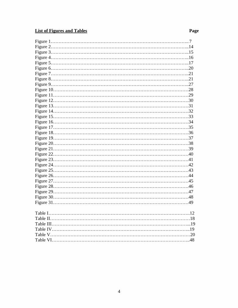
The Paint Branch Stream System is located in the Anacostia watershed network. The Anacostia watershed network comprises the Northwest Branch and Northwest Branches of the Anacostia River. The Northeast Branch, which flows into the Tidal Anacostia, contains the Paint Branch Stream System. The Paint Branch Stream System is comprised of Paint Branch, Little Paint Branch, Indian Creek, and Beaverdam Creek. Indian Creek and Beaverdam Creek are within Beltsville Agricultural Research land and have not been rapidly urbanized as the other two tributaries. Paint Branch Creek and Little Paint Branch Creek join just upstream of the University of Maryland Campus. The study site consists of a site of each of the main upstream tributaries of Paint Branch Creek and four sites downstream of the tributary junction. The NE branch has been gauged by the USGS since 1938.

UMDCampus

500 m

PaintBranchCreek

IndianCreek

Little PaintBranch

Creek

Patronik, 1995

1 2

34

56

Figure 1. Northeast Branch Watershed with inset map showing the main study area (Dr. Prestegaard, 2006). From West to East the main sub-watersheds are Paint Branch Creek, Little Paint Branch Creek, Indian Creek, Beaverdam Creek. The Green line separates the Piedmont from the Coastal Plain. Site 1 is Powdermill Road, site 2 is Cherry Hill Road, site 3 is Jiffy Lube, site 4 is the View, site 5 is Lake Artemesia, and site 6 is College Park airport.

8

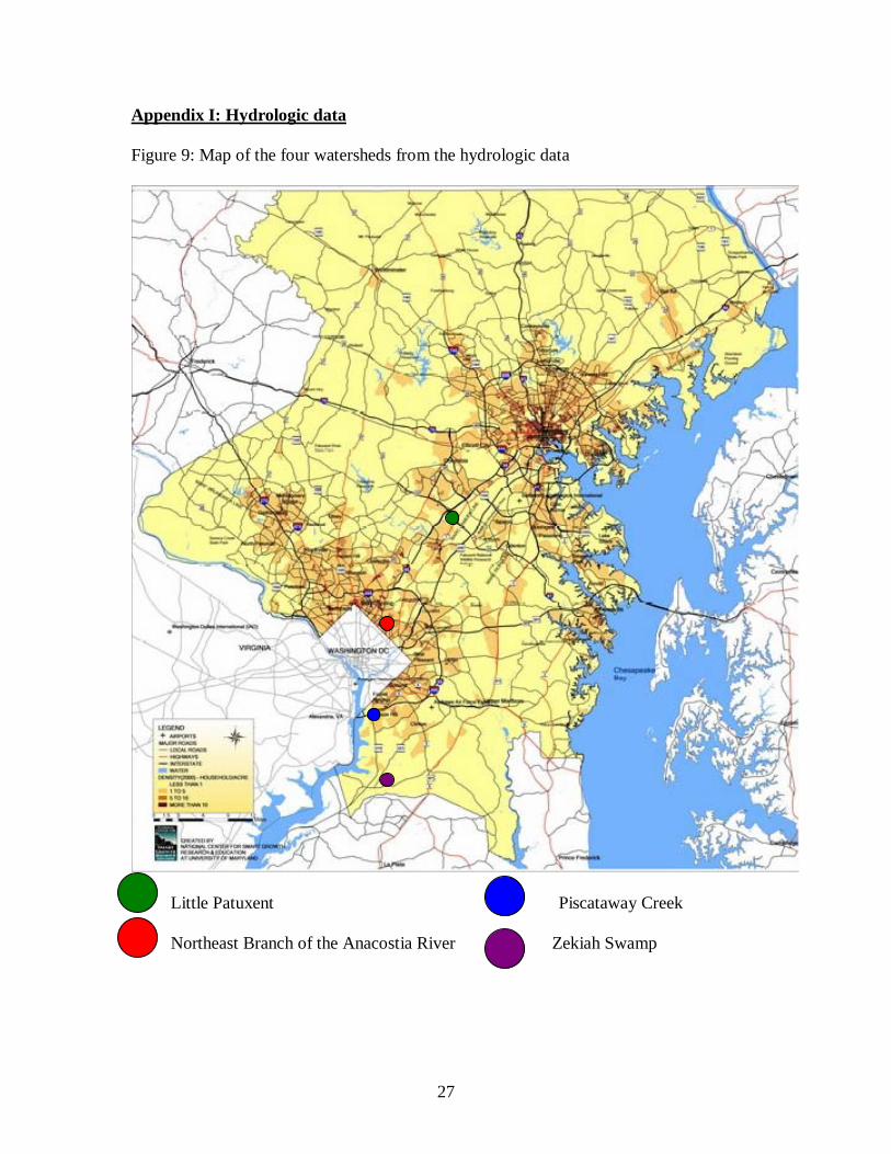
Methods I conducted three main types of data collection and analysis: a) comparison of hydrological databases b) field data collection of channel morphology, and c) data integration and comparison of two existing databases on channel morphology. The first analysis is a hydrological comparison of the changes in the annual maximum flood in the NE Branch of the Anacostia River with three reference streams that have not undergone extensive urbanization. This analysis used existing USGS data and the purpose of this analysis was to determine whether the changes in discharge observed in the NE branch are climatically controlled or due to urbanization. The next series of methods are the field methods explaining how I collected and analyzed channel morphology data. Finally, I compared the field data with two other databases in order to evaluate the amount of change at each site and to explain the morphological change data. Hydrologic Methods The purpose of the hydrological analysis was to determine whether the changes in discharge in the NE Branch were a result of climatic change or urbanization. I used data from four sites gauged by the USGS (Northeast Branch of the Anacostia River, Little Patuxent River, Piscataway Creek, and Zekiah Swamp) to examine changes in the annual peak flood discharge change over time. The Paint Branch Stream lies within the Northeast Branch of the Anacostia watershed, which has been greatly effected by urbanization. However, the three other sites are non-urban stream channels. Therefore, I am able to compare data from gauges located in watersheds adjacent to the Anacostia Watershed. These three non-urban sites were chosen for various reasons. All three sites are mainly located in the Maryland Coastal Plain (Appendix I). They all have gauging stations where discharge is collected, and the peak discharge is recorded. All three sites have a sufficient streamflow record to evaluate flood frequency and records that overlap with the Anacostia in time. The watershed area for each site is similar to that of the Anacostia. In addition, none of these three sites have experienced little or less intense urbanization, which allows for a comparison with the Northeast Branch of the Anacostia. With the data from the four gauged sites, I was able to make many hydrologic analyses and compare them to the morphological analysis at the Paint Branch Stream System. These databases were used for two purposes: a) to evaluate the change in the discharge over time and b) to calculate and estimate the average 2.333-year flood and the bankfull 1.5 year flood. Trend of the Annual Maximum Flood Series The data used to produce the peak floods plots were obtained from the United States Geological Survey (USGS) website. The data I used was the annual maximum peak stream flow for the period of record and the site’s drainage area, which are given in cubic feet per second squared miles. Therefore, I converted the units given to metric units of meters cubed per second and squared kilometers. For each site, I made a graph of the maximum flood peak per year. In order to compare each site to each other I had to

9

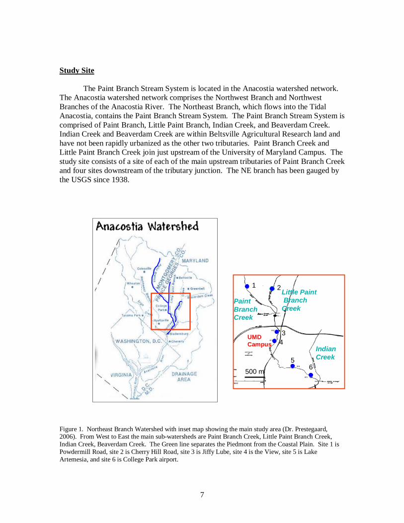
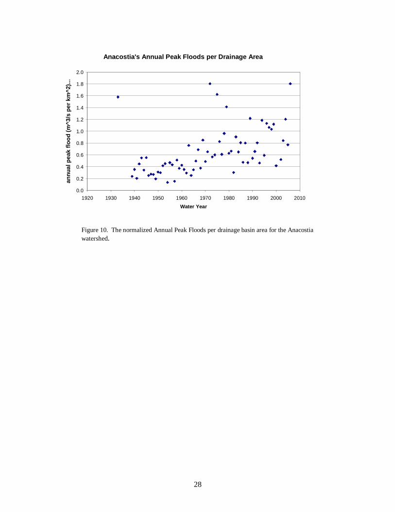
normalize each graph. To normalize the data I divided the peak floods by the drainage area of the system. Then I plotted a graph of flood peaks per drainage area versus the year. Statistically, the mean of the annual flood series is equivalent to the 2.33 recurrence interval (R.I.) flood using annual maximum series data (Dunne and Leopold, 1978). Estimation of the 1.5 year (bankfull) Flood The bankfull flood in many geographical areas has a recurrence interval of 1.5 years. Using the same USGS website and data, I can also produce flood frequency graphs. However, in order to produce an accurate flood frequency curve the data series should be stationary, which implies no change average annual peak flood. There is no discharge change at Piscataway Creek and Zekiah Swamp (Appendix I). There was a small amount of change, however, at Little Patuxent River and a large amount of channel at the NE Branch of the Anacostia. Therefore, the Little Patuxent and NE Anacostia sites were split into two graphs. One graph was from 1933 to 1971 (pre-urban) and the other graph was from 1972 to 2006 (post-urban). For each graph, I sorted the discharge from largest to smallest and placed a rank on each data point where the largest flood is one and so on. Then I calculated the recurrence interval (RI) using the equation RI = (n+1)/rank where n is the number of years of record. Then I plotted the discharge (Q) versus the recurrence interval setting the x-axis as a log scale. Then, in order to compare all four sites to each other I normalized the discharge by the dividing the discharge by the drainage area. I was able to create a graph of discharge per drainage area versus the R.I.

To determine the changes in 1.5 year R.I. with time for the NE branch of the Anacostia, I used three procedures. First I estimated the non-urban bankfull discharge (Q1.5) using a regression equation for Coastal Plain Streams (Prestegaard et al, 2001). This is an equation derived from 15 un-urbanized, gauged stations in the Maryland Coastal Plain.:

Q1.5 = 26.98*D.A..888 (Where D.A. is the drainage basin area in square miles, Q is in cfs.)

Next I used the two flood frequency curves derived from the segmented time series to estimate the 1.5 year flood for the midpoint of the two time segments. The first point, which is the starting point of the line is created using the equation (Prestegaard et al 2001). The second point is the 1.5-year flood extrapolated from the flood frequency curve prior to urbanization. This point was plotted at the midpoint of the range of record at 1952. The last point is the 1.5-year flood extrapolated for the flood frequency curve after urbanization. This point was plotted at the midpoint of the range of record at 1989. Finally, I can estimate the bankfull flood determining the relationship between the average of the annual flood series, which had a recurrence interval of 2.33 years and the 1.5 year flood. To evaluate this relationship I created a dimensionless flood frequency graph of Q/Q1.5 versus the recurrence interval. I took the discharge and divided it by the 1.5-year flood of that data series. I then took the value of Q/Q1.5 for the 2.3 year flood and determined the ratio of the 2.3 year flood to the 1.5 year flood. This provides a

10

continuous estimate of the change in the 1.5 year flood over time by comparison with the average trend of the annual maximum series. Field Channel Morphology Measurements In the field, I resurveyed six sites along the Paint Branch Stream System (Fig. 1). At each site, I surveyed channel cross sections from which I calculated the channel’s width, depth, and area. I also surveyed channel gradient and measured the grain size distribution for each site. The first two sites were sites that Dr. Prestegaard surveyed in 1996. The remaining four downstream sites are resurveys of Daniel Patronik in 1995. Field Measurements of Channel Cross Sections and gradient

In the field, I measured channel bed and bank elevations and depths and the channel width at each survey site. The equipment used was a flexible tape measure, surveyor’s level, stadia rod, and iron rebar to hold the tape measure. At each site, I placed iron rebar at the channel’s bankfull stage. I attached the beginning of the tape measure to the left end looking downstream and pulled it as tightly to the other end. I read the bankfull surface width directly from the tape measure and recorded the value. I walked along the tape measure with the stadia rod stopping every 0.3 m . At these locations, the foresite on the stadia rod was surveyed. Final data set consisted of a set for foresite data that were turned into elevations by subtracting from the height of the instrument. These channel elevation are then used to determine average depth and channel area. From the plotted data, I determined the bankfull height at the site illustrated by a solid line on each cross section (Appendix II). Then to the get the width of the stream, I subtracted the bankfull width from the width even to the bankfull width. The total cross sectional area is the sum of each incremental area across the channel. Average depth was determined by dividing cross sectional area by surface width (Dunne and Leopold, 1978).

At each site, I surveyed water surface elevation that was used to determine channel gradient (change in elevation over distance). In the field, I started upstream and worked my way downstream taking a measurement every two meters. For each measurement, I placed the stadia rod at the surface of the water and the foresite was read from the survey level. Therefore, I was able to obtain elevation at 2 meter increments in the downstream direction. To calculate the gradient, I plotted elevation versus distance downstream and took the absolute value of the slope of the line to determine gradient. Determination of Within-Reach Morphological Variability

To calculate the within reach variability, I measured channel cross sections at each site for a riffle, pool and intermediate cross section. Then I calculated the area, width and depth of each channel and took the average area, width, and depth. From the average, I took the standard deviation in order to get two standard deviations above the mean. I then took two standard deviations above the mean and divided it by the average multiplied by 100 to express variance in percentage. The result provides a measure of the within-reach variance of morphological variables. This provided a standard of

11

channel variation within a reach that could be used to gauge the channel changes that occurred over time.

Surface Grain Size distributions

At each site grain size data were collected and distributions of surface grain size were made. I sampled one hundred particles at each site by walking a grid pattern along each resurveyed cross section. I measured the diameter of the intermediate axis (b-axis) of each grain. These data were analyzed as cumulative grain size distribution from smallest to largest grain size (Fig. 9). The following statistics were determined from the grain size distribution: D50 (the diameter of the median size) and D84 (the diameter of 84th grain size, one standard deviation above the mean). Grain size was used to evaluate relative roughness: depth/D84. These data were used in the determination of the Shield Stress required to move the particles and thus evaluate channel stability. Determination of Channel bed stability

In an evaluation of 24 Piedmont and Coastal Plain stream reaches, Prestegaard

(2001) determined that almost all the non-urban stream channels in this part of Maryland are threshold streams. The definition of a threshold stream is that the bankfull fluid shear stress is within twenty percent of the critical shear stress. The critical shear stress is the critical fluid shear stress at which the bed particles will begin to move. This depends upon the grain size and fluid shear. The critical shear stress is derived from Shields’ criterion, where the coefficient (0.045) is the critical dimensionless shield stress. The value used for critical dimensionless shield stress is a value used for heterogeneous gravel beds (Prestegaard et al., 2001). The equation used to find the critical fluid shear stress is:

τ = .045(ρs-ρw)gD84

where ρs is the density of the solid (2,650 kg/ m3), ρw is the density of water (1000 kg/m3), g is the gravitational acceleration (9.814 m/s2), and D84 is a grain size. The actual shear stress can be determined by the equation τ = ρwgdS where d is the average depth and S is the gradient of the stream. Determination of pre-urban channel morphology

Pre-urban channel morphology was estimated from regional geomorphologic information on Coastal Plain Streams (Prestegaard et al., 2001). These regional relationships are included in Appendix II, and the estimates of the channel dimensions are determined from the watershed area for each cross section site. These channel dimensions are reach-average data derived from 10-12 cross sections per reach, so that they can be compared with cross section data for which the morphological variations are known. The regional characteristics data area presented graphically with the equation of the line provided. Therefore I used the equation from the graph to calculate the channel’s pre-urban width, depth, and area. The equations are as follows:

12

Bankfull width = 8.2877x.4558

Bankfull depth = 1.4998x.6945 Bankfull area = 14.168x.6205 (Dimensions are in ft, ft2 and x is the drainage basin area in square miles).

Evaluation of channel change over time

There are three different time periods that I am using to evaluate the channel change over time. The data for each time period are from different sources, however, each source involves Dr. Prestegaard, which provides consistency in the methods of channel morphology data acquisition. The first set of data calculations are of the pre-urban channel conditions using the reference channels from Maryland Coastal Plain data. The next set of data was calculated in 1995 or 1996 by two different sources. The data at the Cherry Hill and Powdermill sites was collected by Dr. Prestegaard in 1996. The data from the remaining four sites was collected by Daniel Patronik in 1995 for his senior thesis (Appendix II). Finally, the last set of data was collected for this project by Dr. Prestegaard and me in 2006/2007. Therefore, I have three different time intervals with four different sources of the data.

To determine the amount of channel change between each time interval I have three different comparisons (1996-2006, 1960-1996, and 1960-2006). To calculate the amount of change I determined the percent difference for each interval. Therefore, I took the difference in the width, depth, and area for each interval at each site. Then I divided the difference by the area width or depth of the less recent data calculation. Once the amount of percent difference is calculated for all three measures (area, width, and depth) and variability, the type of channel change can be determined at each site. Analysis of Error Survey Error

In my research thesis project I have two main sources of error. The first source of error is the measurement error that I cause. The placement of the stadia rod produces measurement area depending on the bed particles. If the bed is full of small grains then my weight and the weight of the stadia rod could push into the bed. On the other hand if the bed is composed of large particles it depends on where I place the stadia rod. Therefore, the placement of the stadia rod I choose causes the measurement error at each site. I calculated the error at the Cherry Hill Road site because it had small and larger grains within its cross section. In the field I surveyed the original cross section and immediately after I resurveyed the exact same cross section.

13

For the analysis of the error I calculated the channel’s width, depth, and area for each repeated cross section and compared them. I took the difference of the two cross sections for each channel characteristic and divided it by the first survey and multiplied it by 100. These data are illustrated in table I below.

Table I: Measurement Error in Channel Surveys: Cherry Hill Road Measurement Error trial 1 trial 2 diff %diff area 18.3 18.9 0.610 3.34width 17.1 17.1 0.00 0.00depth 1.07 1.11 0.0350 3.27

I produced a percent error of about 3.3 %. This amount of error is insignificant

compared to the amount of change that occurred along the Paint Branch Stream System. The channel width did not change in the survey, but channel depth and thus area both changed from one survey to another due to compaction of loose sediment, variability in the placement of the surveying rod, and other human choices that cause variation in the measurement. Bankfull Estimation Error The other source of error is from the restoration projects at a few of the sites, especially the Jiffy Lube and the View sites. The error is with the determination of the stream’s bankfull, and is one of the reasons why it is often difficult to compare channel morphology data measured by different groups of people. The identification of the stream’s bankfull stage defines the width and depths for the survey. When a stream is surveyed an estimation of the bankfull needs to be consistent at all the sites in order to have an accurate comparison. The View and the Jiffy Lube sites were restored before Dr. Prestegaard and I had the chance to resurvey them. Therefore, we received the data from another source. This source could have placed their bankfull points lower or higher than where Dr. Prestegaard and I would have. Consequently, when I compared the 1996 data to the 2006 data the amount of difference could actually be greater or less than what I calculated. The difference mainly lies with where they placed the estimation of the bankfull channel. Because many of these channels have vertical banks, the error is primarily in the assessment of channel depth. Results and Discussion Hydrological changes in the Anacostia River The amount of discharge flowing in a stream is a major control on the size of the channel. When the distribution of discharges remains constant, the channel form is likely to retain its characteristics. When the discharge regime changes due to a change in climate or an increase in runoff (due to an increase in urbanization and impervious

14

surfaces), then the channel form is also likely to change. I used stream-flow data from the United States Geological Survey (USGS) for four watersheds in the Maryland Coastal Plain to determine whether changes in flood discharges have occurred and to determine whether these changes have been caused by urbanization in the NE branch of the Anacostia River. To determine whether changes in discharge occurred, I examined the magnitude of the annual maximum flood over time for the NE Branch Anacostia station. To test whether any changes in discharge was due to changes in climate rather than urbanization I compared the time series data of discharge for the Anacostia River with three adjacent streams in the Maryland Coastal Plain that had similar watershed areas. Trends in Annual Maximum Flood Peaks

The Anacostia River has experienced an increase in discharge since 1933. The trendline in the graph below illustrates this change. The mean annual flood peak in 1933 is about 50 m3/s. Taking the trend line up to 2006 the mean annual flood peak is about 180 m3/s. The trend line illustrates the change in peak floods from 1993 to 2006, which illustrates that the annual maximum flood series is not stationary.

Figure 2: Trend of the annual maximum Peak flood series for the Anacostia River. (data provided by USGS) The magnitude of the discharge change is illustrated in the graph below. There is an apparent “step” in the middle of the graph around 1972, which is when the Paint Branch Stream System had its major urbanization phase. For each series I inserted lines for the average flood peak at that time. Above those lines I placed dashed lines to illustrate two standard deviations above the mean. The range in between the two lines is the mean annual maximum series for that time series. It is apparent that after

Anancostia River

0

50

100

150

200

250

300

350

400

1920 1930 1940 1950 1960 1970 1980 1990 2000 2010

Year

annu

al fl

ood

peak

(m^3

/s)

15

urbanization the stream experienced a lot of change. The average of the post-urban series is the same as the two standard deviations above the mean for the pre-urban series. Looking at these two series it is evident that the Anacostia watershed was in a quasi-equilibrium state until the urbanization phase in 1972.

Anancostia River

0

50

100

150

200

250

300

350

400

1920 1940 1960 1980 2000 2020Year

annu

al fl

ood

peak

(m^3

/s)

Figure 3: The annual flood peak graph illustrating the step increase due to the urbanization phase around 1972. The average is now above two standard deviation above the mean. Three non-urban sites nearby the Anacostia River show no change in their discharge. The three sites are Little Patuxent River, Piscataway Creek, and Zekiah swamp. These three sites were chosen because they have similar range of record, similar drainage areas, located in the coastal plains of Maryland, and they all have gauging stations where discharge is collected and the peak flood is recorded. The three non-urban sites are graphically portrayed below to illustrate the mean annual flood peak and the annual flood peak per drainage basin area (Appendix I). The non-urbanized watersheds do not show a trend exhibited like the Anacostia River. The fact that the sites adjacent to the Anacostia River show no increase of the annual peak flood indicates that climate change is not the likely explanation for discharge trends within the Anacostia watershed. Therefore, I can conclude that the driving force of the hydrological change is due to the increase of urbanization.

Year

16

Comparison of Non-Urban Streams

0.0

0.5

1.0

1.5

2.0

2.5

3.0

3.5

4.0

1920 1930 1940 1950 1960 1970 1980 1990 2000 2010

Water year (year)

annu

al p

eak

flood

s (m

^3/s

)...

PiscatawayzekiahLittle patuxent

Figure 4: Three nearby watersheds to the Anacostia that show no trend or increase in the discharge over time. Flood Frequency Analysis Flood frequency graphs portray the probability of a particular flood event. The graphs plot the recurrence interval versus the discharge. The recurrence interval depends on the amount of discharge and the time it takes to flow to the nearby stream and watershed. It has been estimated by Leopold and Wolman (1957) that streams adjust themselves to accommodate the 1.5-year flood. The 1.5-year flood occurs as an annual maximum every two or three years, which is a commonly occurring flood event. When there is no urbanization, the 1.5-year flood remains the same. However, when the discharge increases, the stream adapts to the increase and changes its magnitude of the 1.5-year flood. The flood frequency curves (Appendix I) are the Anacostia’s flood frequency graphs for pre-urban and post-urban channel states. When extrapolating values from the graph the 1.5 year flood prior to urbanization gives a discharge of about 53m3/s. After urbanization the 1.5-year flood increases to a discharge of 120 m3/s. From pre-urban to post-urban the Anacostia watershed more than doubled its discharge flow to the streams. Therefore, the stream had to adjust itself to the new and much larger amount of flow. When comparing sites to others I used a normalized flood frequency graph, which incorporates the drainage area of each site. Using these graphs I calculated the discharge of the 1.5-year flood per drainage area prior to urbanization to be .30 m3/s per km2. After urbanization the 1.5-year flood’s discharge per drainage area doubles to .60 m3/s per km2. I compared the flood frequency data of the Anacostia to that of the Piscataway and Little

17

Patuxent (Appendix I). The difference in the discharge per drainage area in the Anacostia River is much larger than the difference in the discharge per drainage area in the Little Patuxent River and Piscataway Creek. Prior to 1971 the Little Patuxent River’s discharge for the 1.5-year flood per drainage area was .28m3/s per km2. After 1972, the discharge per drainage area was .35 m3/s per km2. Piscataway Creek had a discharge of the 1.5-year flood per drainage area of .22 m3/s per km2. The flood frequency data for Piscataway and Little Patuxent compare nicely with the pre-urban data of the Anacostia. However, the post-urban data is quite larger than the data from little Patuxent and Piscataway. The average discharge is around the 2.33-year flood and the bankfull discharge is the 1.5-year flood. The difference between the bankfull discharge and the average discharge could remain the same. For the Anacostia River the average discharge is 1.35 times larger than the bankfull discharge. This relationship is illustrated in the figure below.

Anancostia River

0

50

100

150

200

250

300

350

400

1920 1940 1960 1980 2000 2020Year

annu

al fl

ood

peak

(m^3

/s)

Figure 5: The trendline is the average discharge that is 1.35 times larger than the bankfull discharge, which is the 1.5-year flood. There are many conclusions that can be drawn about the Anacostia watershed from the calculated hydrologic data. One main conclusion is that the Anacostia has a positive trend showing an increase in discharge over time. The non-urbanized streams do not exhibit a trend and their bankfull discharge over time does not change. This comparison suggests that urbanization is reason for the change in discharge on the Anacostia River. Since the discharge increases over time the bankfull discharge increases as well. The bankfull discharge and the average discharge increase together by 1.35. Therefore, you are able to predict the steam’s bankfull and average discharge.

Q Average Q Bankfull

Year

18

Changes in Channel Morphology This section summaries the amount of within-reach morphological variation at two of the stream sites. It also summarizes the field data and illustrates the interval comparisons (pre-urban to 1996 and 1996 to 2006). Finally it provides calculations for what type of streams channel changes are occurring within the Paint Branch Stream System. Within-Reach Morphological Variability The within-reach morphological variability was calculated at Cherry Hill and Powdermill Road. I use these variabilities to determine the type of change that occurred at each site. Table II: Within-Reach Variability Cherry Hill Road Site riffle intermediate pool (trial 1) average 2 std dev variancearea (m2) 16.4 16.6 17.4 16.8 1.08 6.43Width (m) 20.1 18.6 15.4 18.0 4.84 26.8Depth (m) 0.895 0.896 1.13 0.974 0.271 27.8

Powdermill Road Site riffle intermediate pool average 2 std dev variancearea (m^2) 36.5 40.8 33.6 37.0 7.22 19.5width (m) 21.0 24.0 20.0 21.7 4.16 19.2depth (m) 1.74 1.70 1.68 1.71 0.0588 3.45

Estimation of Pre-Urban channel morphology

Pre-urban channel morphology was estimated from regional geomorphologic information on Coastal Plain Streams (Prestegaard et al., 2001). These regional relationships are included in Appendix II, and the estimates of the channel dimensions was determined from the watershed area for each cross section site. These channel dimensions are reach-average data derived from 10-12 cross sections per reach, so that they can be compared with cross section data for which the morphological variations are known.

Pre-urban channel bankfull discharge, Q1.5, can also be estimated from regional relationships for the Maryland Western Coastal Plain (Prestegaard et al., 2001). These relationships can be compared with the data from the NE Branch Anacostia gauging station. If discharge is presented in cubic feet per second (cfs-gauged units), the relationships are as follows for drainage area in square miles: Q1.5 = 26.98D.A.0.888 (Prestegaard et al., 2001). This provides an estimate of the bankfull discharge for the entire NE Branch of 43.7 cfs or 1.24 m3/s. This equation can also be used to estimate bankfull discharge for the contributing tributaries of NE branch illustrated in the table below.

19

Table III: Pre-urban channel characteristics Site name Basin Area, km2 width, m depth, m area, m2 Q1.5, m3/s Powdermill 31.7 7.97 0.78 6.23 7.06 Cherry Hill 26.4 7.28 0.75 5.56 6.01 Golf Course 58.1 10.4 0.90 9.10 12.1 Greenbelt Rd 66.2 11.1 0.90 9.90 13.6 The View 66.7 11.1 0.90 9.90 13.7 Artemesia 81.0 12.1 0.90 11.2 16.3 Airport 87.0 12.5 1.00 11.7 17.3

Evaluation of Channel Changes from pre-urban to 1996 The channel changes from pre-urban to 1996 were assessed by comparing the calculated pre-urban conditions to Prestegaard’s and Patronik’s data in 1996 for each site. A summary of the 1996 channel characteristics and the percent difference from the pre-urban to 1996 is presented in Table IV (below). These data indicate significant variation for changes from the pre-urban conditions to the 1996 conditions. The amount of change calculated from pre-urban to 1996 illustrates the transformational change the channels went through during the major urbanization phase on the Paint Branch Stream System. Table IV Channel change: Pre-urban to 1996

Site name width (m) % difference Depth (m) % difference area (m^2)

% difference Powdermill Road 19.2 141 1.53 97.2 29.4 372Cherry Hill Road 14.0 92.3 1.21 62.4 17.0 205Golf Course 28.0 169 0.81 10.0 22.7 149Jiffy Lube 45.5 310 1.22 35.6 55.5 466The View 35.0 215 1.61 78.9 56.4 470Lake Artemesia 31.5 160 0.65 27.8 20.5 83.0Airport 29.5 136 1.02 2.00 30.1 157

Evaluation of Channel Changes from 1996 to 2006 The channel changes from 1996-2006 are assessed by comparing channel morphological change from repeated surveys. The survey conducted by Prestegaard and Patronik in 1996 were compared to the resurvey of that site by Prestegaard and me. An example of the repeated surveys is shown in the summary data Table V.

20

Table V Channel change: 1996 to 2006 Site name width (m) % difference Depth (m) % difference area (m^2) % difference Powdermill Road 21.0 9.38 1.74 13.6 36.5 24.2 Cherry Hill Road 15.3 9.29 1.14 -6.02 17.4 2.46Jiffy Lube 46.3 1.82 1.40 14.9 64.9 17.0The View 47.2 35.0 1.21 -24.3 57.6 2.13Lake Artemesia 36.9 17.1 1.05 60.8 38.5 88.0Airport 29.0 -1.84 1.24 21.9 35.8 19.0

Channel Characteristics change over time I graphically illustrated these interval changes for each channel characteristic (width, depth and area). Therefore, you are able to visually see the changes that have occurred along the Paint Branch Stream System pre-urbanization to the present. In general the most amount change occurred in the widths for each site.

Width change over time

0

5

10

15

20

25

30

35

40

45

50

1970 1975 1980 1985 1990 1995 2000 2005 2010

time (year)

wid

th (m

)

Powdermill RdCherry Hill RdJiffy LubeThe ViewLake ArtemesiaAirport

Figure 6: Width Change over time intervals (pre-urban to 1996 and 1996 to 2006) at all six resurveyed sites.

21

Depth Change over time

0

0.2

0.4

0.6

0.8

1

1.2

1.4

1.6

1.8

2

1970 1975 1980 1985 1990 1995 2000 2005 2010

time (year)

Dep

th (m

)

Powdermill RdCherry HillJiffy LubeThe ViewLake ArtemesiaAirport

Figure 7: Depth Change over time intervals (pre-urban to 1996 and 1996 to 2006) at all six resurveyed sites.

Change in Area over time

0

10

20

30

40

50

60

70

1970 1975 1980 1985 1990 1995 2000 2005 2010

time (year)

Are

a (m

^2)

Pwdermill RdCherry Hill RdJiffy LubeThe ViewLake ArtemesiaAirport

Figure 8: Area Change over time intervals (pre-urban to 1996 and 1996 to 2006) at all six resurveyed sites.

22

Channel Stability Changes Prior to urbanization all the sites along the Paint Branch Stream System were threshold sites (Prestegaard et al., 2001). Therefore, I calculated the shear stress at an upstream site (Cherry Hill Road) and a downstream site (the airport) to see if any of the sties were still threshold sites. Using the equations explained before the critical shear stress was 29.8 N/m2. The actual shear stress right now at Cherry Hill is 107 N/m2. The critical shear stress for the airport is 32.7 N/m2. The actual shear stress presently at the airport is 165 N/m2. Both sites are way above threshold by 70 to 80 percent. Therefore, none of the sites are threshold sites as they likely were prior to urbanization.

Even though Powdermill and Cherry Hill are not threshold sites I still calculated the morphological variation within the channel reach because both sites are at equilibrium with their sediment deposition. The channel area, width, and depth are shown in Table II. These data are consistent with the amount of within-reach variability identified by Prestegaard et al, (2001) from a data set of 20 sites with more extensive cross sectional measurements of within-reach variability. Conclusions

By using the annual maximum flood data, I was able to illustrate the change in peak floods per year at the Anacostia River. I was also able to show the lack of change on non-urban sites nearby the Anacostia River. The difference of having a trend at the Anacostia River and no trend at the three non-urban sites indicates that urbanization was the likely cause for the increase of floods along the NE branch of the Anacostia. The flood frequency analysis allows the before and after bankfull discharge estimation. The flood frequency curves show how much the 1.5-year flood changed before and after urbanization, which was about a 50 percent increase. The flood frequency curves also allow the Anacostia to be compared to the other non-urban sites, which are summarized in Prestegaard (2001).

Prior to urbanization all of the streams along the Paint Branch Stream System were threshold streams. However, using calculations of shear stress I found that what were once threshold streams are now way above threshold streams. The change in stream channels are also expressed in the comparison interval, especially from pre-urban to 1996. This time interval showed a huge amount of channel change with increased width by well over 100 percent. The large increase in channel widths was also illustrated in the large change of the channel areas. Therefore, since urbanization there has been a large amount of transformational change where the stream channel has widened and deepened at almost all locations. Thus, most of the stream channel morphology within the study reach indicated transformational change, which resulted from the shifting of the channels from threshold streams, to streams that moved and stored significant amounts of sediment along the channel system.

The amount of difference between 1996 and 2006 varied significantly among the sites. At the two upstream tributaries, the Cherry Hill Road and the Powdermill Road

23

sites, the amount of morphological change was within the range of with-in reach morphological variation. At the downstream locations, the complexity of the gravel bars made it difficult to evaluate the within-reach morphological variability. Evaluation of the change falls within the calculated amount of variance allowed for the stream at Cherry Hill in 2006. The comparison from 1996 to 2006 demonstrates the stream has been in a quasi-equilibrium channel state upstream of the convergence of Paint Branch and Little Paint Branch. The four downstream sites are not consistent with a quasi-equilibrium channel state. Therefore, the upstream data supports Hammer’s previous work and literature as well as my hypothesis for my research project. However, the downstream sites are exhibiting changes that are not consistent with a quasi-equilibrium channel.

Discussion Hammer’s 1972 paper about channel changes in an urban watershed suggested that channel form would enlarge to convey the post-urban bankfull discharges. In Hammer’s 1972 study of Piedmont streams in Pennsylvania, however, the channels enlarged primarily by increasing their width, not their depths. Therefore, these Piedmont streams could remain threshold channels. In this study of the Maryland Coastal Plain, however, the channels enlarged both the widths and the depths. This increase in depth caused a significant increase in bankfull shear stress and thus the mobility of the sediment in the channel. Bedload transport rates greatly increase with shear stresses in excess of the critical shear stress.

When the channel change over time is examined in the Paint Branch Creek Watershed, it indicates significant changes since the non-urban condition, but also significant changes since 1995-1996. The evaluation of sediment mobility indicates that all of the streams were above the threshold of motion, indicating that the streams have transformed from threshold channels to channels that must maintain equilibrium not by maintaining stable channel banks, but by moving sediment into the reach to replace sediment eroded from the reach. This change from threshold to above threshold channels has caused a large change in channel morphology with huge gravel bars at all 4 downstream sites, which help to drive channel change.

I also found that our main method of measuring morphological variation by comparing riffles and pools was appropriate for threshold channels or channels with little stored sediment. The channels that had large gravel bars, which were all the sites except for the first two, did not exhibit simple pools and riffles, and therefore, this procedure could not be used. Therefore, we had to compare each 1995 survey site directly with the 2006 resurveyed site. When streams have developed complex channels bars as the Paint Branch stream system has it is very difficult to measure the amount of within-reach morphological variation. In addition, when streams are restored (e.g. on campus) no variation can be determined because the stream was changed unnaturally.

24

Acknowledgements I would first like to thank my advisor, Dr. Karen L. Prestegaard for all her help and support in my senior thesis project. She helped me in the field as well as the analysis of the field data. She also gave me very helpful pointers to write this and other papers throughout the year. Another person who helped me in the field was Robert Thomas, a fellow geology student, who helped me collect data when Dr. Prestegaard was not available. I would also like to thank my parents who always support and encourage me throughout all my endeavors. I would also like to thank my dad for editing my final paper at the last moment.

25

Bibliography

Abernethy, B., Rutherfurd, I.D., 1998, Where along a River’s Length Will Vegetation Most Effectively Stabilise Stream Banks; Geomorphology, vol. 23, p.55-75 Ashmore, P.E., Richard, P.S., 2003, The Relation Between Particle Path Length Distributions and Channel Morphology in Gravel-bed Streams; Geomorphology, v. 56, no. 1-2, p. 167-187 Chin, A., 2006, Urban Transformation of River Landscapes in a Global Context; Geomorphology, v. 79, no. 3-4, p. 460-487 Doyle W., Shield, D., January 2000, incorporation of Bed Texture into a Channel Evolution Model; Geomorphology, vol. 34, p. 291-309 Hammer, 1972, Stream channel enlargement due to Urbanization; Water Resources, Research v. 8, no. 6, pp. 1530-1540 Kondolf, G.M., et al., October 2002, Channel Response to Increased and Decreased Bedload Supply from Land Use Change: Contrasts Catchments; Geomorphology, vol.45, p.35-51 Langbein, W.B., and Leopold, Luna B., 1964, Quasi-Equilibrium States in Channel Morphology; American Journal of Science, v.262 (June), p.782-794 Leopold, L.B. and Maddock, T., 1953, The Hydraulic Geometry of Stream Channels and Some Physiographic Implications; Geological Survey Professional Paper 252, p. 1-57 Leopold, L. B., and Wolman, M.G., 1957, River Channel Patterns: Braided, Meandering and Straight, U.S. Geological Survey Professional Paper 282-B, 51p Leopold, L.B., October 1970, An Improved Method for Size Distribution of Stream Bed Gravel; U.S. Geological Survey, Water Resources Research, vol. 6, no. 5, p. 1357-1366 Leopold, L. B., 1973, River Channel Change with Time – An Example; Geological Society of America Bulletin, v.84, p.1845-1860. Leopold, L.B., 1992, Sediment Size that Determines Channel Morphology; Dynamics of Gravel Bed Rivers, v. 14, p. 297-311 Leopold, L.B., et al., 2005, Direct Observation of Rates of Geomorphic Change: 41 Years of Direct Observation; American Philosophical Society Proceedings. Patronik, D.C., August 1995, Sediment Supply Changes in the Paint Branch Stream

26

Prestegaard, K.L., Dusterhoff, S., Houghton, K., Clancy, K., and Stoner, E., 2001, Hydrological and geomorphologic characteristics of Piedmont and Coastal Plain Streams, MD: Maryland Department of Environment Report. Rinaldi, M., Simon, A., 2006, Disturbance, Stream incision, and Channel Evolution: The Roles of Excess Transport Capacity and Boundary Materials in Controlling Channel Response; Geomorphology, v. 79, no. 3-4, p. 361-383 Wellmeyer, J.L. et al., February 2005, Quantifying Downstream Impacts Of Impoundment of Flow Regime and channel platform, Lower Trinity River, Texas; Geomorphology , vol. 69, p. 1-13

27

Appendix I: Hydrologic data Figure 9: Map of the four watersheds from the hydrologic data

Little Patuxent Piscataway Creek Northeast Branch of the Anacostia River Zekiah Swamp

28

Anacostia's Annual Peak Floods per Drainage Area

0.0

0.2

0.4

0.6

0.8

1.0

1.2

1.4

1.6

1.8

2.0

1920 1930 1940 1950 1960 1970 1980 1990 2000 2010Water Year

annu

al p

eak

flood

(m^3

/s p

er k

m^2

)...

Figure 10. The normalized Annual Peak Floods per drainage basin area for the Anacostia watershed.

29

Flood Frequency for the Anacostia from 1933-1971

0

50

100

150

200

250

300

350

1 10 100

Recurrance Interval (years)

Q (m

^3/s

)

Figure 11. The pre-urban flood frequency graph for the Anacostia Watershed.

30

Flood Frequency for the Anacostia from 1972-2006

0

50

100

150

200

250

300

350

400

1 10 100

Recurrence Interval (years)

Q (m

^3/s

)

Figure 12. The flood frequency graph after urbanization at the Anacostia Watershed

31

Flood Frequency curve per Drainge Area from 1933-1971

0

0.2

0.4

0.6

0.8

1

1.2

1.4

1.6

1.8

1 10 100

Recurrance Interval (years)

Q (m

^3/s

) per

km

^2

Figure13. The normalized pre-urban flood frequency graph for the Anacostia River

32

Flood Frequency curve per Drainage Area from 1972-2006

0

0.2

0.4

0.6

0.8

1

1.2

1.4

1.6

1.8

2

1 10 100

Recurrance Interval (years)

Q (m

^3/s

) per

km

^2

Figure 14. The normalized flood frequency graph after urbanization for the Anacostia River.

33

Flood Frequency per Km ^2

0.0

0.5

1.0

1.5

2.0

2.5

1 10 100

Recurrance interval (years)

Q p

er k

m^2

Figure 15. The normalized flood frequency graph for Piscataway

34

1933 to 1971 per drainage area at little Patuxent

0.0

0.2

0.4

0.6

0.8

1.0

1.2

1.4

1.6

1.8

1.0 10.0 100.0

Recurrance interval (years)

Q (m

^3/s

) per

km

^2...

.

Figure 16: The pre-urban normalized floor frequency graph for Little Patuxent River

35

1972 to 2006 per drainage area at Little Patuxent

0

0.5

1

1.5

2

2.5

3

3.5

4

1 10 100

Recurrence Interval

Q (m

^s/s

) per

km

^2...

Figure 17. The normalized flood frequency graph after urbanization for Little Patuxent River.

36

Appendix II: Morphological Data

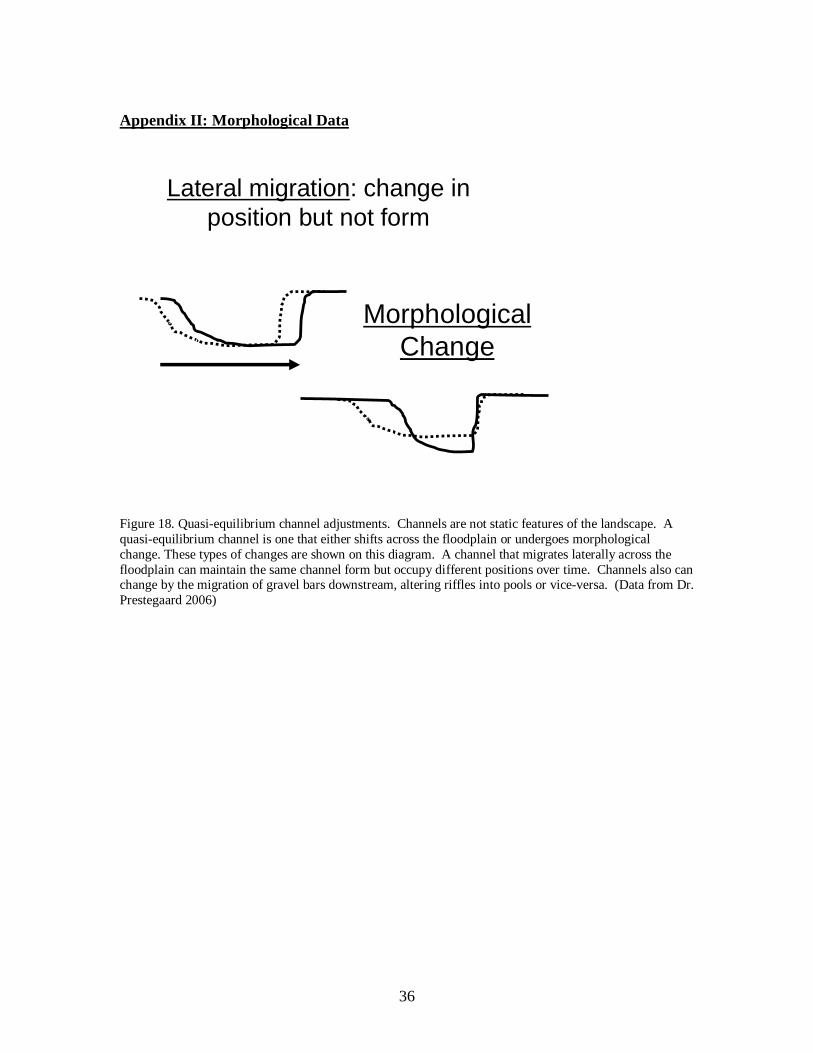
Lateral migration: change in position but not form

Morphological Change

Figure 18. Quasi-equilibrium channel adjustments. Channels are not static features of the landscape. A quasi-equilibrium channel is one that either shifts across the floodplain or undergoes morphological change. These types of changes are shown on this diagram. A channel that migrates laterally across the floodplain can maintain the same channel form but occupy different positions over time. Channels also can change by the migration of gravel bars downstream, altering riffles into pools or vice-versa. (Data from Dr. Prestegaard 2006)

37

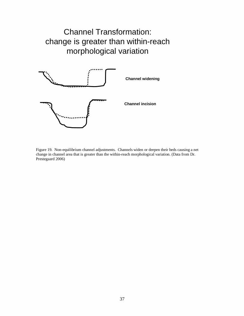
Channel Transformation: change is greater than within-reach

morphological variation

Channel widening

Channel incision

Figure 19. Non-equilibrium channel adjustments. Channels widen or deepen their beds causing a net change in channel area that is greater than the within-reach morphological variation. (Data from Dr. Prestegaard 2006)

38

Identify 2 outliers + 1 averageNorth Creek: Depth vs. Distance DS

0

0.5

1

1.5

0 20 40 60 80 100 120

D is ta nc e D S (m )

Mean depth = 0.89 m; Standard deviation = 0.18 m

Figure 20. Because streams do not have random arrangement of channel characteristics, stratified sampling one riffle, one pool, one average part of the channel can be sampled and these 3 cross sections can be averaged to obtain reach-average characteristics. Compare mean and standard deviations with previous diagram. (Data from Dr. Prestegaard 2006)

39

COASTAL PLAINy = 8.2877x0.4558

R2 = 0.8599

1

10

100

0.1 1 10 100

DRAINAGE AREA, sq. mi.

BA

NK

FULL

WID

TH, f

t

Figure 21. Regional characteristics of stream channels for the width in the Piedmont and Coastal Plains of Maryland prior to the affects of urbanization. Diagrams from Prestegaard et al., 2001.

40

COASTAL PLAIN STREAMSy = 1.4998x0.2112

R2 = 0.6945

0.1

1

10

0.1 1 10 100

DRAINAGE AREA, sq. mi.

DEP

TH, f

t

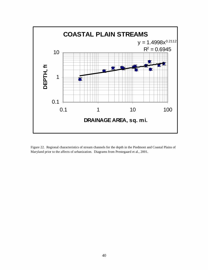
Figure 22. Regional characteristics of stream channels for the depth in the Piedmont and Coastal Plains of Maryland prior to the affects of urbanization. Diagrams from Prestegaard et al., 2001.

41

COASTAL PLAIN STREAMSy = 14.168x0.6205

R2 = 0.7601

1

10

100

1000

0.1 1 10 100

DRAINAGE AREA, sq. mi.

CH

AN

NEL

AR

EA, s

q. ft

Figure 23. Regional characteristics of stream channels for the area in the Piedmont and Coastal Plains of Maryland prior to the affects of urbanization. Diagrams from Prestegaard et al., 2001.

42

Figure 24: Scanned image of Daniels Patronik’s cross section for the four downstream sites (Jiffy Lube, the View, Lake Artemesia, and the airport).

Site: Golf Course

Site: Jiffy Lube

Site: The View

Site: Lake Artemesia

Site: Airport

43

comparision between 2 cross sections

-2-1.8-1.6-1.4-1.2

-1-0.8-0.6-0.4-0.2

0

0 5 10 15 20

distance (m)

dept

h (m

)

Trial 1Trial 2

Figure 25. Graphically illustrating the error variability of the repeated Cherry Hill site. (Data from the field in the fall of 2006)

44

Cross Section At Cherry Hill (2006)

-2-1.8-1.6-1.4-1.2

-1-0.8-0.6-0.4-0.2

0

0 5 10 15 20 25

distance (m)

dept

h (m

)

Pool 1Pool 2riffleintermediate

Figure 26. Graphically comparing the calculated cross section of Cherry Hill in 2006, illustrating the riffle, pool, and intermediate sections. (Data from the field in fall of 2006)

45

All three surveys at Powdermill Road

-3

-2.5

-2

-1.5

-1

-0.5

0

0.5

0 5 10 15 20 25 30

Width (m)

Dep

th (m

)

riffleintermediatepool

Figure 27. Graphically comparing the calculated cross section of Powdermill Road in 2006, illustrating the riffle, pool, and intermediate sections. (Data from the field in spring of 2007)

46

Comparision from 1996-2006

-2

-1.8

-1.6

-1.4

-1.2

-1

-0.8

-0.6

-0.4

-0.2

0

0.2

0 2 4 6 8 10 12 14 16 18

width (m)

Dep

th (m

))

19962006

Figure 28. Comparison of the Cherry Hill site from 1996 to 2006. (Data from Dr. Prestegaard 1996 and fieldwork in 2006)

47

Appendix III: Grain Size Distributions

cherry hill 2006 pebble count

0

10

20

30

40

50

60

70

80

90

100

1 10 100 1000

radius of B axis (mm)

Cum

ulat

ive

perc

ent

Figure 29. The grain size distribution at Cherry Hill in 2006. Below are the values of D50 and D84 in 1996 and 2006. Grain Size 2006 1996 D84 (mm) 41 32 D50 (mm) 23 22

48

Grain Size distributions for Jiffy Lube grain size 1996 2006 D84 (mm) 113 62 D50 (mm) 71 33

Grain size distributions for the View grain size 1996 2006 D84 (mm) 90 58 D50 (mm) 76.7 32

Table VI: The values for Jiffy Lube and the View grain size. Data was provided by the University of Maryland geomorphologic class prior to the restoration.

49

Pebble Count for Site 4: Airport

0

10

20

30

40

50

60

70

80

90

100

1 10 100 1000

diameter of the b-axis (mm)

cum

ulat

ive

perc

ent

Figure 30: Grain size distribution for site 4: Lake Artemesia. Below are values of the D84 and D50 for 1996 and 2006. grain size 1996 2006 D84 (mm) 108 22 D50 (mm) 60.2 11

50

Pebble Count for Site 5: Airport (riffle)

0

10

20

30

40

50

60

70

80

90

100

1 10 100 1000

diameter of b-axis (mm)

cum

ulat

ive

perc

enta

ge

Figure 31. The grain size distribution for site 5: the airport. Below are values of the D84 and D50 for 1996 and 2006. grain size 1996 2006 D84 (mm) 52.5 45 D50 (mm) 41.2 26