DEGREE PROJECT, IN , FIRST LEVELCOMPUTER SCIENCESTOCKHOLM, SWEDEN 2015

Evaluating a fractal features methodfor automatic detection of Alzheimer’sDisease in brain MRI scansA QUANTITATIVE STUDY BASED ON THEMETHOD DEVELOPED BY LAHMIRI ANDBOUKADOUM IN 2013

FILIP SCHULZE AND LOVISA RUNHEM

KTH ROYAL INSTITUTE OF TECHNOLOGY

SCHOOL OF COMPUTER SCIENCE AND COMMUNICATION

Evaluating a fractal features method forautomatic detection of Alzheimer’s Disease in

brain MRI scans

A quantitative study based on the method developed by Lahmiri and Boukadoum in2013

FILIP SCHULZE AND LOVISA RUNHEM

Bachelor’s Thesis in Computer Science at CSCSupervisor: Pawel HermanExaminer: Örjan Ekeberg

Abstract

The field of computer-aided diagnosis has recently madeprogress in the diagnosing of Alzheimer’s disease (AD) frommagnetic resonance images (MRI) of the brain. Lahmiriand Boukadoum (2013) have research this topic since 2011,and in 2013 they presented a system for automatic detec-tion of AD based on machine learning classification. Theirproposed system achieved a classification accuracy of 100%(2013, p. 1507) using support vector machines with quadratickernel classifiers. The MRI scans were first translated to1-dimensional signals, from which three features were ex-tracted to measure the signals self-a�nity. These three fea-tures were Hurst’s exponent, the total fluctuation energy ofa detrended fluctuational analysis and the same analysis’scaling exponent. The results of their study were validatedusing a dataset of 23 MRI scans from brains with AD andnormal brains.

This report makes an attempt at implementing the methodproposed by Lahmiri and Boukadoum in 2013 and evaluat-ing its accuracy on a dataset of 120 cases, out of which 60are cases of AD and 60 are normal cases. The results werevalidated using both leave-one-out cross-validation and 3-fold cross-validation. A dataset of 23 cases consistent withLahmiri and Boukadoum’s in size was considered and thelarger dataset of 120 cases. The best classification accu-racy for the small and large were obtained from the 3-foldcross-validation was 78,26% respectively 65,00%.

The results of this study are to some extent similar tothose of Lahmiri and Boukadoum’s, however this study failsto verify how their method performs on a larger dataset, astheir results for a small dataset could not be reproducedin this implementation. Thus the results of this report areinconclusive in verifying the accuracy of the implementedmethod for a larger dataset. However this implementationof the method shows promise as the accuracy for the largedataset was fairly good when comparing to other researchdone in the field.

Referat

Området datorstödd diagnos har nyligen gjort framstegnär det gäller diagnostik av Alzheimers sjukdom (AD) frånmagnetresonansbilder (MRI) i hjärnan. Lahmiri och Bou-kadoum (2013) har forskat i ämnet sedan 2011, och 2013presenterade de ett system för automatisk detektering avAD, som bygger på maskininlärningsklassificering. Derasföreslagna system uppnådde en klassificeringsnoggrannhetpå 100 % (2013, s. 1507) med hjälp av stödvektormaskinermed kvadratiska kärnor. MRI:er blev först översatta till en-dimensionella signaler, från vilken tre utmärkande faktorersom mäter signalens själv samhörighet extraherades. De trefaktorerna var Hurst exponent, den totala fluktuationsener-gin hos en detrenderad fluktuationsanalys och skalningsex-ponenten gavs av samma analys. Resultaten av deras studievaliderades med en datamängd bestående av 23 MRI frånhjärnor med AD och normala hjärnor.

Denna rapport gör ett försök till att implementera me-toden utvecklad av Lahmiri och Boukadoum under 2013,och utvärdera dess riktighet på en datamängd av 120 fall,varav 60 är fall av AD och 60 är normalfall. Resultaten vali-derades med både lämna-ett-ute korsvalidering och 3-faldigkorsvalidering. En datamängd av 23 fall, som är förenligmed Lahmiri och Boukadoums storlek, och en större data-mängd av 120 fall prövades. De bästa korrekthetsvärdenaför den mindre och större datamängderna som erhölls från3-faldig korsvalidering var 78,26% respektive 65,00%.

Resultaten av denna studie är i viss mån förenliga medLahmiri och Boukadoums resultat, men denna studie lyc-kades inte bekräfta att deras metod fungerar på en störredatamängd, eftersom deras resultat för en liten datamängdinte kunde återskapas i denna implementering. Således ärresultaten av denna rapport inte övertygande i att kontrol-lera riktigheten i den implementerade metoden för en störredatamängd. Men denna implementering av metoden visarpotential, eftersom noggrannheten för den stora datamäng-den var relativt bra när vid jämförelse med annan forskningsom gjorts inom området.

Contents

1 Introduction 21.1 Problem definition . . . . . . . . . . . . . . . . . . . . . . . . . . . . 31.2 Scope and constraints . . . . . . . . . . . . . . . . . . . . . . . . . . 31.3 Outline . . . . . . . . . . . . . . . . . . . . . . . . . . . . . . . . . . 3

2 Background 52.1 Alzheimer’s Disease . . . . . . . . . . . . . . . . . . . . . . . . . . . 5

2.1.1 Mild cognitive impairment . . . . . . . . . . . . . . . . . . . . 62.2 State-of-the-art analysis for CAD for AD . . . . . . . . . . . . . . . 72.3 Technical background . . . . . . . . . . . . . . . . . . . . . . . . . . 8

2.3.1 Magnetic resonance imaging and computer-aided diagnosis . 82.3.2 Extraction of fractal features . . . . . . . . . . . . . . . . . . 92.3.3 Support vector machines and classification . . . . . . . . . . . 102.3.4 Lahmiri & Boukadoun’s methodology . . . . . . . . . . . . . 10

3 Metod 123.1 Data and datasets . . . . . . . . . . . . . . . . . . . . . . . . . . . . 12

3.1.1 Acknowledgement . . . . . . . . . . . . . . . . . . . . . . . . 133.2 Technical approach . . . . . . . . . . . . . . . . . . . . . . . . . . . . 13

3.2.1 Transforming the MRI to a 1-dimensional signal . . . . . . . 143.2.2 Feature extraction . . . . . . . . . . . . . . . . . . . . . . . . 153.2.3 Feature classification . . . . . . . . . . . . . . . . . . . . . . . 16

3.3 Validation of results . . . . . . . . . . . . . . . . . . . . . . . . . . . 163.3.1 Leave-one-out cross-validation . . . . . . . . . . . . . . . . . . 163.3.2 3-fold cross-validation . . . . . . . . . . . . . . . . . . . . . . 17

4 Results 184.1 1-dimensional signals of MRI scans . . . . . . . . . . . . . . . . . . . 184.2 Computation time . . . . . . . . . . . . . . . . . . . . . . . . . . . . 194.3 Classification accuracy . . . . . . . . . . . . . . . . . . . . . . . . . . 19

4.3.1 Leave-one-out cross-validation . . . . . . . . . . . . . . . . . . 204.3.2 3-fold cross-validation . . . . . . . . . . . . . . . . . . . . . . 22

5 Discussion 24

5.1 Discussion on the data used . . . . . . . . . . . . . . . . . . . . . . . 255.2 Discussion on the method implemented . . . . . . . . . . . . . . . . 26

6 Conclusion 28

7 References 29

Support acknowledgement

Data used in preparation of this article were obtained from the Alzheimer’s DiseaseNeuroimaging Initiative (ADNI) database (adni.loni.usc.edu). As such, the inves-tigators within the ADNI contributed to the design and implementation of ADNIand/or provided data but did not participate in analysis or writing of this report. Acomplete listing of ADNI investigators can be found at: <http://adni.loni.usc.

edu/wp-content/uploads/how_to_apply/ADNI_Acknowledgement_List.pdf>Data collection and sharing for this project was funded by the Alzheimer’s Dis-

ease Neuroimaging Initiative (ADNI) (National Institutes of Health Grant U01AG024904) and DOD ADNI (Department of Defense award number W81XWH-12-2-0012). ADNI is funded by the National Institute on Aging, the National Insti-tute of Biomedical Imaging and Bioengineering, and through generous contributionsfrom the following: AbbVie, Alzheimer’s Association; Alzheimer’s Drug DiscoveryFoundation; Araclon Biotech; BioClinica, Inc.; Biogen; Bristol-Myers Squibb Com-pany; CereSpir, Inc.; Eisai Inc.; Elan Pharmaceuticals, Inc.; Eli Lilly and Company;EuroImmun; F. Ho�mann-La Roche Ltd and its a�liated company Genentech,Inc.; Fujirebio; GE Healthcare; IXICO Ltd.; Janssen Alzheimer ImmunotherapyResearch & Development, LLC.; Johnson & Johnson Pharmaceutical Research &Development LLC.; Lumosity; Lundbeck; Merck & Co., Inc.; Meso Scale Diagnos-tics, LLC.; NeuroRx Research; Neurotrack Technologies; Novartis PharmaceuticalsCorporation; Pfizer Inc.; Piramal Imaging; Servier; Takeda Pharmaceutical Com-pany; and Transition Therapeutics. The Canadian Institutes of Health Researchis providing funds to support ADNI clinical sites in Canada. Private sector con-tributions are facilitated by the Foundation for the National Institutes of Health(www.fnih.org). The grantee organization is the Northern California Institute forResearch and Education, and the study is coordinated by the Alzheimer’s DiseaseCooperative Study at the University of California, San Diego. ADNI data aredisseminated by the Laboratory for Neuro Imaging at the University of SouthernCalifornia.

1

Chapter 1

Introduction

The idea of using computers for diagnosing diseases emerged during the 20th cen-tury, and since then the field of computer-aided diagnosis (CAD) has emerged andfacilitated the diagnosing of many medical conditions and diseases. Specifically, asubfield of how to correctly diagnose Alzheimer’s disease (AD) has been vastly re-searched the last decade. AD is a chronic neurodegenerative disease and a form ofdementia. The disease is caused by the gradual death of cells in the brain, givingsymptoms that gradually get worse. Symptoms are bad short-term-memory, prob-lems understanding language, and di�culty in achieving everyday tasks (Aquilo-nius). Since the symptoms are not very distinguished, and it still is debatablewhich symptoms are to be counted to AD, the disease can be di�cult to discover,especially in its early stages. About 100’000 people in Sweden have AD and thecost of care for them is approximated to 63 billion SEK (Aquilonius). Moreover,diagnosing the disease can be both expensive for society and uphold the quality oflife for patients and their friends and family.

During the last years many articles have been published on the field of ap-plication for using CAD to diagnosing AD. To apply the resources of computersto analyzing data collected in the diagnosing process, such as magnetic resonanceimaging (MRI) scans, opens up for new possibilities and challenges. The fact thata computer e�ectively can analyze data, in ways that humans cannot, has made itpossible to investigate relationships between di�erent components in the collecteddata. Correlations between components can be investigated, and since a computercan process images as well as applying algorithms to the result these possibili-ties have been thoroughly investigated the last years. Many of these attempts tofind methods for diagnosing AD with CAD have resulted in complex algorithmsthat rely on great computer resources. However Lahmiri and Boukadoum (2013)have developed a simpler approach to the problem than those previously presented.Their research applies a new method (Lahmiri and Boukadoum, 2013.) to a datasetconsisting of 23 MRI scans and obtains 100% classification accuracy. Their CADsystem is notably less complex than many others proposed, and proved to be ef-ficient in processing time as well. However, their method was never tested on a

2

1.1. PROBLEM DEFINITION

larger dataset, hence their study has paved a path for future experiments. Sincemost other CAD systems are complex to implement and leave room for error alongthe processing chain, the method developed by Lahmiri and Boukadoum has anadvantage in being relatively simple. Their impressive accuracy obtained in thestudy from 2013 (p. 1507) adds promise to the CAD system developed. Since thedataset was very small the system needs to be tested on a larger dataset to see howwell the performance, in terms of accuracy of diagnosis, scales in a larger study.This report aims to implement the method developed by Lahmiri and Boukadoumin 2013, and test the approach on a dataset consisting of 127 MRI scans.

1.1 Problem definitionThis study will investigate how well the system for diagnosing AD developed byLahmiri and Boukadoum in 2013 scales to a larger problem domain. In other wordsthis report will aim to evaluate whether the accuracy of their method of classificationcan be established for a larger dataset, as it was only validated by using a total of23 brain MRI scans.

1.2 Scope and constraintsThe focus of this report is to implement a method as consistent as possible towardsthat developed by Lahmiri and Boukadoum in 2013. Thus, the correlation betweenthe method and the level of accuracy obtained in the results of this study will beevaluated, in an attempt to verify the performance of the method on a large dataset.

Finally, the purpose of the whole field of CAD for AD is to achieve a way ofaccurately diagnosing AD. Owing to the methods accuracy in diagnosing AD, canwe know whether the method is a suitable one to distinguish normal brain MRIscans from MRI scans of brains with AD? In this study a binary classification willbe performed on the MRI scans used, meaning that either the cases are classified asnormal or they are classified as cases of AD. The proposed system of diagnosis willnot be able to determine how early the algorithm can discover AD. Consequently,mild cognitive impairment (MCI) – although relevant to the research of AD – isconsidered to be outside of the scope of this study and will thus not be consideredin the classification step. MCI is however relevant to the research of AD and willtherefore be mentioned in this report.

1.3 OutlineThis thesis introduces the research previously presented by Salim Lahmiri andMounir Boukadoum with the purpose to copy their method developed in 2013.In the background AD and MCI is presented together with the state-of-the-art inCAD for AD. Furthermore, a background about the Machine Learning methodsused is given. The previous work by Lahmiri and Boukadoum is also accounted

3

CHAPTER 1. INTRODUCTION

for along with their original data. In methods the data used in this study is ac-counted for, and then the implementation is described in depth. The results aredivided into the graphic representations of the 1-dimensional signals, computationtime and classification accuracy obtained by the system developed. The part aboutclassification accuracy is divided by the result of the leave-one-out cross validationand 3-fold cross validation. In the discussion general points about the study is firstraised, then there is a part with a deeper discussion about the data used, followedby a deeper discussion on the implementation. Finally the conclusion of the studyis presented.

4

Chapter 2

Background

The aim of this background is to introduce the notions, concepts and techniqueswhich are used in this study. In 2.1 dementia and AD are described. The points ofinterest are how the disease progresses and what the symptoms are. In 2.2 MCI isshortly explained. In 2.3 state-of-the-art in CAD for dementia and AD is presented.The main source is the paper by Bron E.E et al. summarizing the CAD dementiagrand challenge. In 2.4 we introduce the technical concepts needed for our study.First of all what a MRI is and how it can be used in CAD. Then an introduction tothe extraction of fractal features is given. That includes what Detrended fluctuationanalysis (DFA) is and what Hurst’s exponent is. The last part in the technicalbackground is about classification with a Support Vector Machine (SVM). Lastlyin 2.5 a recap on Lahmiri and Boukadoum’s most recent work is given, with focuson their study in 2013.

2.1 Alzheimer’s DiseaseDementia is a term that describes a range of symptoms indicating a loss of function-ality in the brain (Nationalencyklopedin, 2009). It is often associated with a declinein memory skills, and there are many di�erent forms of dementia. Dementia canbe caused by damage to the brain or caused by a disease, and to what extent thediseases are genetically inherited can also vary. However, the symptoms of demen-tia diseases are often similar, as they often cause reduced memory loss, problemscommunicating through language and problems achieving everyday tasks.

AD is a form of dementia (Nationalecyklopedin, 2009) that today is considered tobe a collection of very similar conditions and diseases. AD also deteriorates causingnew and more severe symptoms over time. That is why an early diagnosis improvesthe possibilities of a good care for the patient (alz.org, n.d). Overall the a�ectedperson can appear to be very confused, and in the early stages of the disease peopleclose to the a�ected often mistake the symptoms for normal aging (Medicinenet,2015). However, AD is not a normal part of aging but a medical condition.

AD is caused by nerve cells losing their ability to function and eventually, during

5

CHAPTER 2. BACKGROUND

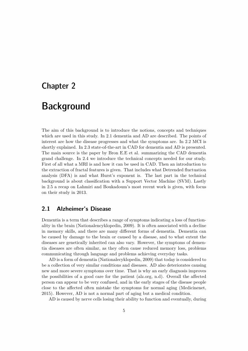
the decline of the disease, the nerve cells die. The presence of AD starts in thefrontal lobe and then spreads to other parts of the brain. The frontal lobes arethe memory centers of the brain, which is why bad short-term memory is such acommon symptom that presents early.

Figure 2.1. AD progressing in a human brain (alz.org, n.d).

The exact reason for why AD breaks out is not yet identified. However, it isknown that in brains a�ected by AD there are proteins that create neurofibrillarytangles in, and between, nerve cells and amyloid plaques (Nationalencyklopedin,2009). That is how nerve cells are disturbed to lose function and eventually die.The plaque has a core of the protein beta-amyloid and is surrounded by damagedor dead nerve cells. Even though it is not certain these plaques and tangles arebelieved to be the cause of AD.

Figure 2.2. Normal brain to the left, AD brain to the right, displayed in doublecolor format to enhance the di�erence between normal brain MRIs and AD brainMRIs (Harvard Medical School webpage, n.d cited in Lahmiri and Boukadoum, 2013,p. 1508).

2.1.1 Mild cognitive impairmentMild cognitive impairment (MCI) is a reduction of a person’s cognitive abilitiesthat is more prominent than the e�ect of normal aging, however not as severe as to

6

2.2. STATE-OF-THE-ART ANALYSIS FOR CAD FOR AD

classified as dementia. It does not a�ect the ability of performing everyday tasks,and at present day MCI is not formally considered a medical diagnosis. It hassimilar symptoms to dementia but does not cause as severe impairments, howeverit is a common yet unconfirmed hypothesis that MCI often evolves into dementia(Nationalecyklopedin, n.d).

2.2 State-of-the-art analysis for CAD for AD

CAD is and has been a subject of research since the 1950s. Applying it for diagnosingAD has for the last few years been a growing subfield. In 2015 Bron E.E et alpublished a paper (Bron E.E et al, 2015) summarizing the first results of the CADdementia grand challenge. The challenge was announced in 2014 and contains 29algorithms from 15 international research teams. The challenge was specified todevelop algorithms for diagnosing AD using MRIs as data. In the conclusions ofthe report they claim “The framework defines evaluation criteria and provides apreviously unseen multi-center data set with the diagnoses blinded to the authors ofalgorithms” (Bron E.E et al, 2015). Bron E.E et al. (2015, p.15) state that whetherthey have collected the best algorithms in the field is unsure. To participate in thechallenge was very demanding, on top on the task of developing an algorithm forCAD Dementia, therefore some teams with good solutions may have chosen notto participate. However the paper provides the first tests where the algorithms donot execute on data very similar to the data it has been trained with. This givesa first insight to what the algorithms would be like in actual clinical situations.The best algorithm had a 63% accuracy. 19 out of 29 algorithms had an accuracybetween 45% and 55%, out of which three algorithms performed worse, and sevenperformed better. The Sørensen-equal algorithm was the best algorithm in theCAD dementia challenge and the only one with a resulting accuracy of over 60%.Since there are not many other comparative studies in the field it is not sure ifthere are better algorithms than those submitted in the competition or not. Therewas no trend found in what classifiers make the best algorithms, so there is nostandardization in this area yet. Although all the algorithms in the CAD-Dementiachallenge use MRIs as data, they use di�erent features that can be extracted fromthe MRIs. Some algorithms combined features and other used only one, but it wasconcluded that the best performing algorithms combined di�erent features. Themost commonly used features extracted from the MRIs were volume, thickness andshape of the brain. Intensities of the images was a common feature, although lesscommon than the previously mentioned ones. The databases used in the measuringand testing were ADNI and AIBL (AIBL, cited in Bron E.E et al, 2015, p.6). Eventhough most of the recent algorithms discovered in the field involve distinguishingand diagnosing MCI in patients, the CAD dementia challenge did not address thatissue (Bron E.E et al, 2015). Therefore the algorithms were only tested on theirabilities to diagnose dementia.

Lahmiri and Boukadoum have since 2011 published di�erent papers on how

7

CHAPTER 2. BACKGROUND

to diagnose AD by classifying brain MRIs using machine-learning techniques. In2011 they published the paper “Brain MRI classification using an ensemble systemand LH and HL wavelet sub-bands features”, where they presented an entirely newmethod to classify healthy brain MRIs and those with abnormalities (Lahmiri andBoukadoum, 2011). The features they used to analyze the MRI were LH and HLsub-bands and first order statistics. The classification was done with a combinationof k-nearest neighbor, learning vector quantization, probabilistic neural networksand support vector machines. As their work has progressed it has become morespecialized. In the paper “Automatic brain MR images diagnosis based on edgefractal dimension and spectral energy signature” (Lahmiri and Boukadoum, 2012)they tried to adjust the algorithms to find di�erent pathologies in brain MRI, amongthem Alzheimer’s Disease. In 2013 they published the paper “Automatic Detectionof AD in Brain Magnetic Resonance Images Using Fractal Features” (Lahmiri andBoukadoum, 2013) in which a simpler approach was presented when comparingwith other available algorithms. During the development they have become morespecialized towards diagnosing AD. To make sophisticated algorithms for that aimthey have changed some of their mathematical methods. In 2013 other featureswere extracted from the MRIs than in 2011. A few features and functionalitywere kept, for example MRI images were still analyzed and SVMs are still used forclassification.

2.3 Technical backgroundThis section provides the background for the technical aspects of the report andstudy.

2.3.1 Magnetic resonance imaging and computer-aided diagnosisMagnetic resonance imaging (MRI) is a noninvasive medical test that aids physiciansto diagnose and treat medical conditions. When performing an MRI scan on thebrain powerful magnetic pulses and radio wave energy are used to create an imageof the brain and the surrounding nerve tissue is created (WebMD, 2012). In thediagnosing of AD an MRI is often used to rule out other diseases that may causesymptoms similar to those of AD, since an MRI can reveal tumors, strokes, build-upof fluid, damage and indications of severe trauma on the head (alz.org, n.d). As ADis characterized by gradual loss of neurons and synapses this can cause a change inthe brain’s tissue and geometrical features (Wenk G.L, 2003 cited in Lahmiri andBoukadoum, 2013, p.1506).

Since the brain’s tissue and geometrical features change during the progressionof AD it is possible to investigate how di�erent features can be used for CAD ofAD. In simple terms the di�erences created by AD have a visual component in thescans, and therefore di�erent features present in these scans can be used in theCAD. As explained in the state-of-the-art analysis, a wide range of features havebeen researched and tested against each other. Once a feature or a group of features

8

2.3. TECHNICAL BACKGROUND

that have significance for the diagnosing of AD have been identified, these featuresfrom the basis for the computer classification of the original MRI scan. The featurescan be combined in a feature vector, and by using machine learning techniques thisfeature vector can be used to detect patterns and correlations between the featuresand how the di�erences correspond to di�erent diagnoses. The aim for the machinelearning system used is to learn to classify the data originating from healthy brains,as well as those of patients with AD, and correctly diagnosing a patient based onthis data.

2.3.2 Extraction of fractal features

A fractal is a geometric shape that is self-similar and has fractional dimensions(Kale and Butar Butar, 2015). Fractal features can be used to measure both self-similarity and local, global and long-range power-law correlations in signals. Whenexamining a MRI scan fractal features are present, but di�cult to analyze. However,by transforming the MRI scan to a 1-dimensional signal, it is possible to extractfractal features by the means of signal analysis. The geometrical features of theoriginal scan are represented by deviations in the resulting signal. Thus, if thedi�erences of AD brains and normal brains are present in the MRI scans thesedi�erences could translate to the 1-dimensional signal.

The Hurst exponent is a fractal feature, and can be extracted from a 1-D signal asdescribed in the previous paragraph. Hurst exponent describes the scaling behaviorof a signal, namely the range of cumulative deviations from the signals mean (Kaleand Butar Butar, 2015). It is directly related to the fractal dimension, whichmeasures the smoothness of a surface or a time series (Lahmiri and Boukadoum,2013, p. 1506).

DFA is a method developed by a C.-K Peng et al. (1994). Today it is know as amethod for determining the statistical self-a�nity of a signal, and has proven usefulin revealing the extent of long-range correlations in time series (Physionet.org). Itis similar to Hurst’s exponent, however DFA can also be applied to signals whoseunderlying statistics, such as mean and variance, or dynamics are non-stationary.DFA can also serve as a complement to Hurst’s exponent, as it evaluates an image’sroughness. When applying DFA on the 1-D signal explored in the previous sectionthe fractal stability of the MRI with regard to scale changes is evaluated, and thusit can be considered to analyzing the image roughness according to the originalhypothesis proposed by Lahmiri and Boukadoum. The result of the DFA on the1-D signal is a scaling exponent and the energy of the detrended fluctuations of thesignal. Lahmiri and Boukadoum hypothesize that AD reduces the spread of pixelintensity in the MR image su�ciently to decrease its self- similarity in comparisonto white noise or a normal MR image (Lahmiri and Boukadoum, 2013). Thus,they also conclude that the scaling exponent should be di�erent from the obtainedHurst’s exponent, and that this method should be able to distinguish an healthybrain from one with AD using the appropriate classifiers.

9

CHAPTER 2. BACKGROUND

2.3.3 Support vector machines and classificationSupport vector machines (SVMs) are supervised learning models within the fieldof machine learning. SVMs apply learning algorithms to analyze data and learn torecognize patterns in the dataset. The theory behind SVMs was developed in the1960s and was first introduced by Vapnik and Chervonenkis (columbia.edu), andis based on statistical learning theory. SVMs are commonly used, and known fortheir good performance, in bioinformatics (Byvatov and Schneider, 2003), text andimage processing among other fields of application. SVMs are trained to identifypatterns by feeding them with test data, in which the input data to be processed iscorrelated to the expected outcome. Based on this training SVMs can be used toclassify new data, and has thus been thoroughly used in a lot of research focusingon the uses of CAD for diagnosing AD with a high level of accuracy. A SVM is wellsuited for solving two-class classification problems, and does this by constructingoptimal separating hyper-planes so as to maximize the distance between the twonearest data points in the two classes.

2.3.4 Lahmiri & Boukadoun’s methodologyIn Lahmiri and Boukadoun’s recent work they have started by transforming theMRI image into a 1-dimensional (1-D) signal, on which they can perform a signalanalysis and investigate di�erent features in the signal. In their paper from 2014they make the hypothesis that a healthy brain MRI would present with more reg-ularity, in this context less rough or jagged edges, than that of a brain with ADor MCI (Lahmiri and Boukadoum, 2014. page 34). The method that we are im-plementing is from their paper on “Automatic Detection of Alzheimer Disease inBrain Magnetic Resonance Images Using Fractal Features”, published in 2013. Inthis paper they propose a simpler approach, that leads to a faster running algo-rithm than many others that we have come across in the state-of-the-art analysis(Bron E.E et al, 2015). In short their method can be described as transformingthe brain MRI scan to a 1-D signal without doing any image preprocessing. Thenthey extract two features from the obtained signal by using detrended fluctuationanalysis, and together with Hurst’s exponent for the 1-D signal a three-componentvector is formed. This vector consisting of three fractal features is feed to the SVMwith quadratic kernels – which perform the classification. In this paper they con-clude that the proposed methodology using SVMs with quadratic kernels had 100%detection accuracy, however the dataset only consisted of a small sample of MRIscans (twenty-three).

Data used in the original study

The original study performed by Lahmiri and Boukadoum was validated using adataset of 23 T2 weighted brain MRIs that were collected from the Harvard MedicalSchool database (2013, p. 1507). The images were all in gray scale and the imagesize was 256x256. Out of the 23 brain MRIs 10 were of normal brains and 13 were

10

2.3. TECHNICAL BACKGROUND

of brains with AD. In their paper from 2013 they make no statement of whether thefull set of scans for all patients were considered, or if only one scan per patient wasused in the analysis. Since their paper only mention 1-D signals of a MRI scan, itis assumed that only individual scans are analyzed when performing the diagnosis.

11

Chapter 3

Metod

This section describes the method of the report and the technical implementationof the techniques previously explained.

3.1 Data and datasets

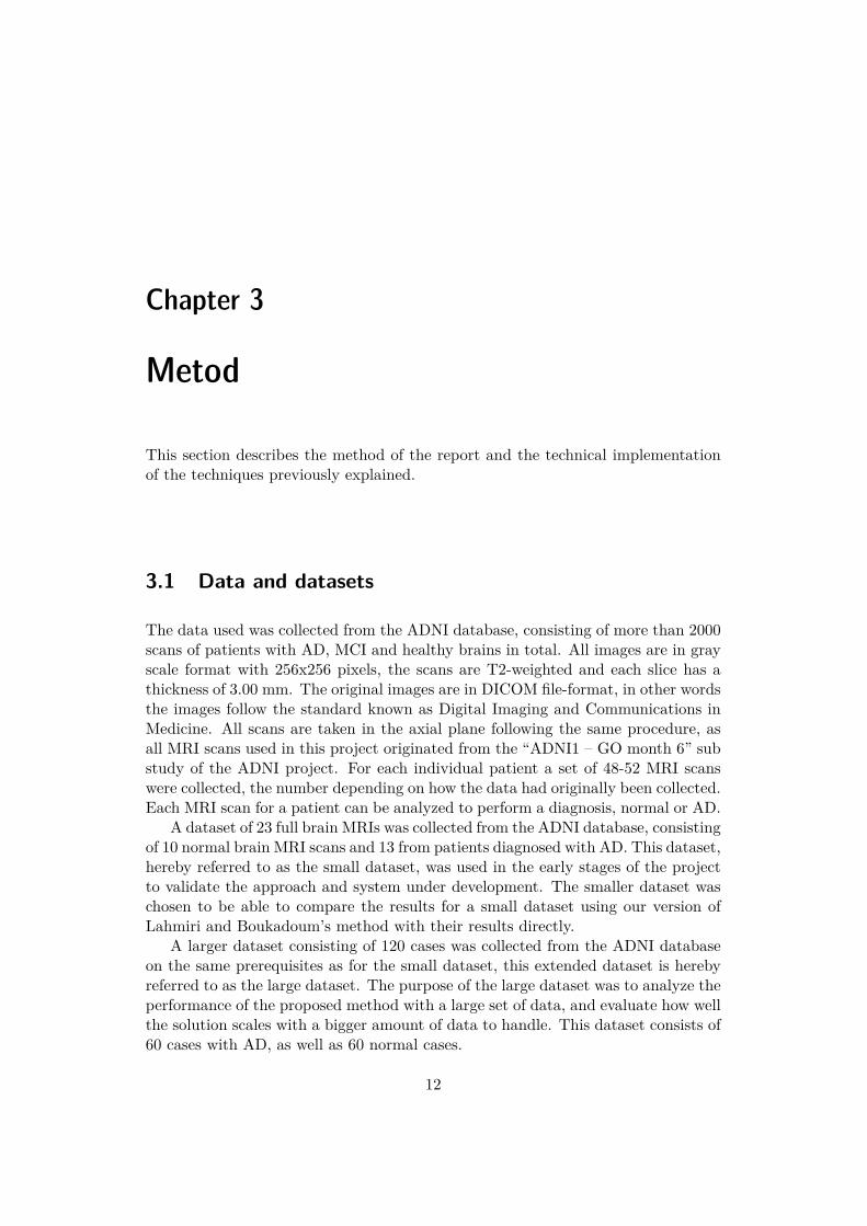
The data used was collected from the ADNI database, consisting of more than 2000scans of patients with AD, MCI and healthy brains in total. All images are in grayscale format with 256x256 pixels, the scans are T2-weighted and each slice has athickness of 3.00 mm. The original images are in DICOM file-format, in other wordsthe images follow the standard known as Digital Imaging and Communications inMedicine. All scans are taken in the axial plane following the same procedure, asall MRI scans used in this project originated from the “ADNI1 – GO month 6” substudy of the ADNI project. For each individual patient a set of 48-52 MRI scanswere collected, the number depending on how the data had originally been collected.Each MRI scan for a patient can be analyzed to perform a diagnosis, normal or AD.

A dataset of 23 full brain MRIs was collected from the ADNI database, consistingof 10 normal brain MRI scans and 13 from patients diagnosed with AD. This dataset,hereby referred to as the small dataset, was used in the early stages of the projectto validate the approach and system under development. The smaller dataset waschosen to be able to compare the results for a small dataset using our version ofLahmiri and Boukadoum’s method with their results directly.

A larger dataset consisting of 120 cases was collected from the ADNI databaseon the same prerequisites as for the small dataset, this extended dataset is herebyreferred to as the large dataset. The purpose of the large dataset was to analyze theperformance of the proposed method with a large set of data, and evaluate how wellthe solution scales with a bigger amount of data to handle. This dataset consists of60 cases with AD, as well as 60 normal cases.

12

3.2. TECHNICAL APPROACH

Figure 3.1. Five images from a sequence of 48 illustrating the layers in which thescans are taken. The scan is of a patient with AD (ADNI-database, 2006).

3.1.1 Acknowledgement

Data used in the preparation of this article were obtained from the Alzheimer’sDisease Neuroimaging Initiative (ADNI) database (adni.loni.usc.edu). The ADNIwas launched in 2003 as a public-private partnership, led by Principal InvestigatorMichael W. Weiner, MD. The primary goal of ADNI has been to test whetherserial magnetic resonance imaging (MRI), positron emission tomography (PET),other biological markers, and clinical and neuropsychological assessment can becombined to measure the progression of mild cognitive impairment (MCI) and earlyAlzheimer’s disease (AD). For up-to-date information, see www.adni-info.org.

3.2 Technical approachThe system analyzes one MRI scan in order to perform a diagnosis on the patientusing SVM classifiers. Since there is a collection of scans for each patient 5 di�erentlayers of the brain will be analyzed and the results evaluated. The scan beinganalyzed is first transformed into a 1-D signal and thus represented by a row vectorin the technical implementation. From this signal the three fractal features areextracted and together they form the three-component feature vector needed forthe SVM classifier.

13

CHAPTER 3. METOD

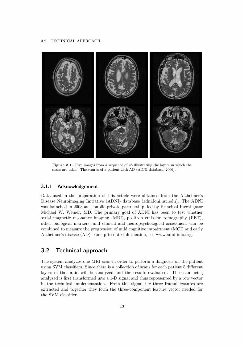
The three features extracted are Hurst’s exponent, the total fluctuation energyof a performed DFA and the scaling exponent of the same analysis. The threefeatures are collected in a feature vector, in which each row vector represents acase. A SVM implementation is used from MATLAB’s library and used to classifythe data. The SVMs were set up with quadratic kernel classifiers and validated byboth leave-one-out cross-validation and 3-fold cross-validation.

Figure 3.2. An overview of the method applied.

3.2.1 Transforming the MRI to a 1-dimensional signalThe method explored by Lahmiri and Boukadoum is based on signal analysis. TheMRI scans used are transformed into 1-D signals, from which the features used inclassification are extracted. Their dataset consisted of 23 images in gray scale, and

14

3.2. TECHNICAL APPROACH

these images were transformed into a 1-D signal by applying row concatenation(Lahmiri and Boukadoum, 2013. p. 1507). No image preprocessing is needed priorto transforming the image to a signal. In gray scale the image can be interpretedas values representing the intensity in each of the positions in the image. Whenthe image is transformed into a signal this can be done with di�erent results inthe resulting signal, in other words the level of how accurate the signal is towardsthe original image can vary. This level of accuracy depends on how the manypositions in the image that are collected into a data point in the resulting matrixrepresentation of the image. In Lahmiri and Boukadoum’s study the highest levelof accuracy was obtained as each pixel in the MRI scans were represented as datapoints in the matrix representation. Lahmiri and Boukadoun also concluded thatthe result of their study persisted even when the 1-D signal was obtained by columnconcatenation, however this is not validated in this study.

In this study all MRI scans were transformed to 1-D signals using a MATLABscript that was implemented according to Lahmiri and Boukadoum’s methodology.Since each person has a collection of brain MRI scans the signals for each scantogether form a matrix that is subject to the feature extraction in the next stepof the implementation. The collection of scans for each person is first ordered inaccordance to the level in which the scans were taken, i.e. from the neck up tothe top of the head. This was done prior to forming the matrix to ensure that thedi�erent cases were treated consequently in this study.

3.2.2 Feature extractionSince Lahmiri and Boukadoum (2013, p. 1607) hypothesize that AD reduces thespread of pixel intensity su�ciently to decrease its self similarity, features measuringthe self-similarity of the signal are chosen in the applied method. Therefore Hurst’sexponent and two features from a DFA are extracted, as they provide a measure ofboth the self-a�nity as well as local, global and long-range deviations of the signalsanalyzed.

Hurst’s exponent

In Lahmiri and Boukadoum’s from paper of 2013 (p. 1506) section 2a they de-scribe how they implemented Hurst’s exponent. However in this study the general-ized Hurst’s exponent (Matteo, 2007), implemented in MATLAB, was used instead(Aste, 2013). The generalized Hurst’s exponent was extracted from the 1-D-signalsrepresenting a MRI by treating the signal as a time series.

Alpha component and total fluctuation energy

DFA is performed on the matrix containing the 1-D signals for each case used in thestudy. The analysis detects long-range power-law correlations in the fluctuationsof a signal treated as a time series. The alpha component computed by DFA isthe scaling component and can be regarded as a measure that is similar to Hurst’s

15

CHAPTER 3. METOD

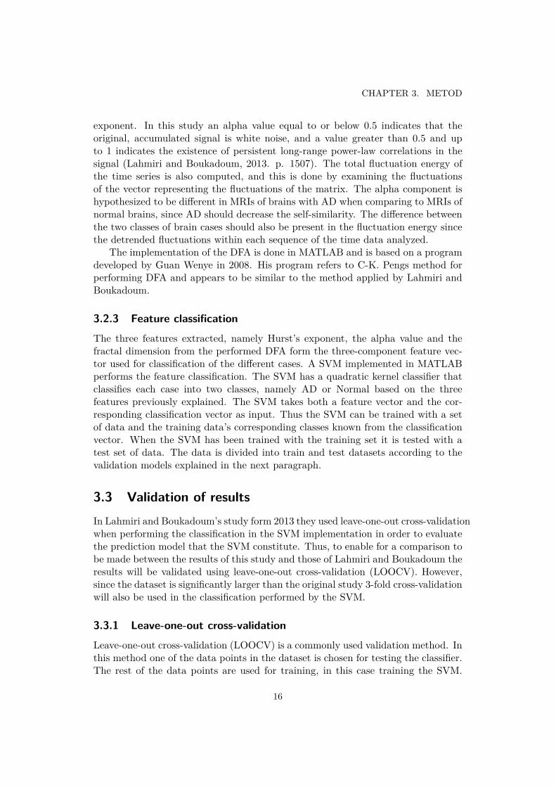
exponent. In this study an alpha value equal to or below 0.5 indicates that theoriginal, accumulated signal is white noise, and a value greater than 0.5 and upto 1 indicates the existence of persistent long-range power-law correlations in thesignal (Lahmiri and Boukadoum, 2013. p. 1507). The total fluctuation energy ofthe time series is also computed, and this is done by examining the fluctuationsof the vector representing the fluctuations of the matrix. The alpha component ishypothesized to be di�erent in MRIs of brains with AD when comparing to MRIs ofnormal brains, since AD should decrease the self-similarity. The di�erence betweenthe two classes of brain cases should also be present in the fluctuation energy sincethe detrended fluctuations within each sequence of the time data analyzed.

The implementation of the DFA is done in MATLAB and is based on a programdeveloped by Guan Wenye in 2008. His program refers to C-K. Pengs method forperforming DFA and appears to be similar to the method applied by Lahmiri andBoukadoum.

3.2.3 Feature classificationThe three features extracted, namely Hurst’s exponent, the alpha value and thefractal dimension from the performed DFA form the three-component feature vec-tor used for classification of the di�erent cases. A SVM implemented in MATLABperforms the feature classification. The SVM has a quadratic kernel classifier thatclassifies each case into two classes, namely AD or Normal based on the threefeatures previously explained. The SVM takes both a feature vector and the cor-responding classification vector as input. Thus the SVM can be trained with a setof data and the training data’s corresponding classes known from the classificationvector. When the SVM has been trained with the training set it is tested with atest set of data. The data is divided into train and test datasets according to thevalidation models explained in the next paragraph.

3.3 Validation of resultsIn Lahmiri and Boukadoum’s study form 2013 they used leave-one-out cross-validationwhen performing the classification in the SVM implementation in order to evaluatethe prediction model that the SVM constitute. Thus, to enable for a comparison tobe made between the results of this study and those of Lahmiri and Boukadoum theresults will be validated using leave-one-out cross-validation (LOOCV). However,since the dataset is significantly larger than the original study 3-fold cross-validationwill also be used in the classification performed by the SVM.

3.3.1 Leave-one-out cross-validationLeave-one-out cross-validation (LOOCV) is a commonly used validation method. Inthis method one of the data points in the dataset is chosen for testing the classifier.The rest of the data points are used for training, in this case training the SVM.

16

3.3. VALIDATION OF RESULTS

The trained SVM is then tested with the one chosen data point. The procedureis repeated until all the data points have been used for testing the classifier, thusthe method assures that all data points are used for testing and the training setis as large as possible in each iteration (Schneider, 1997). Because of the exhaus-tive nature of this method in assuring the largest possible test set, this method ofvalidation is often applied for small datasets.

3.3.2 3-fold cross-validation3-fold-cross-validation is very closely related to LOOCV. The data points are notchosen one by one, but divided into three sets. Then the same procedure as inLOOCV is repeated, but instead of a single element one of the three sets is chosenand used for testing. The procedure is repeated until all three sets have been usedfor testing (Schneider, 1997).

17

Chapter 4

Results

The following sections present the results of this study, gathered according to thepreviously described method.

4.1 1-dimensional signals of MRI scans

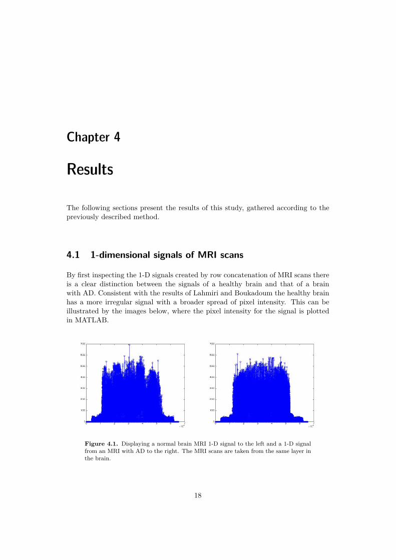
By first inspecting the 1-D signals created by row concatenation of MRI scans thereis a clear distinction between the signals of a healthy brain and that of a brainwith AD. Consistent with the results of Lahmiri and Boukadoum the healthy brainhas a more irregular signal with a broader spread of pixel intensity. This can beillustrated by the images below, where the pixel intensity for the signal is plottedin MATLAB.

Figure 4.1. Displaying a normal brain MRI 1-D signal to the left and a 1-D signalfrom an MRI with AD to the right. The MRI scans are taken from the same layer inthe brain.

18

4.2. COMPUTATION TIME

4.2 Computation timeThe feature extraction processing time was approximately 106 seconds per caseusing MATLAB_R2014bc� on a 2.6 GHz Intel Core i7 processor on Mac OS X10.9.4. Performing the DFA is the most time consuming process during the featureextraction, and takes approximately 102 seconds per case.

4.3 Classification accuracyThe below sections present the accuracy of the classification performed by theSVM using the two di�erent validation methods. For both the leave-one-out cross-validation and the 3-fold cross-validation the numbers and measures presented hereare extracted using the classperf function in MATLAB, which evaluates the perfor-mance of the SVM classifier.

19

CHAPTER 4. RESULTS

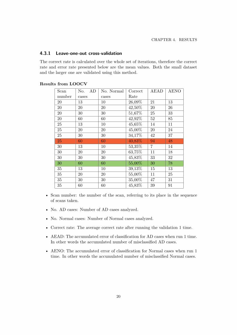
4.3.1 Leave-one-out cross-validationThe correct rate is calculated over the whole set of iterations, therefore the correctrate and error rate presented below are the mean values. Both the small datasetand the larger one are validated using this method.

Results from LOOCVScannumber

No. ADcases

No. Normalcases

CorrectRate

AEAD AENO

20 13 10 26,09% 21 1320 20 20 42,50% 20 2620 30 30 51,67% 25 3320 60 60 42,92% 52 8525 13 10 45,65% 14 1125 20 20 45,00% 20 2425 30 30 34,17% 42 3725 60 60 40,83% 94 4830 13 10 53,35% 7 1430 20 20 63,75% 11 1830 30 30 45,83% 33 3230 60 60 55,00% 30 7835 13 10 39,13% 15 1335 20 20 55,00% 11 2535 30 30 35,00% 47 3135 60 60 45,83% 39 91

• Scan number: the number of the scan, referring to its place in the sequenceof scans taken.

• No. AD cases: Number of AD cases analyzed.

• No. Normal cases: Number of Normal cases analyzed.

• Correct rate: The average correct rate after running the validation 1 time.

• AEAD: The accumulated error of classification for AD cases when run 1 time.In other words the accumulated number of misclassified AD cases.

• AENO: The accumulated error of classification for Normal cases when run 1time. In other words the accumulated number of misclassified Normal cases.

20

4.3. CLASSIFICATION ACCURACY

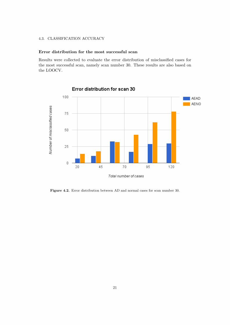
Error distribution for the most successful scan

Results were collected to evaluate the error distribution of misclassified cases forthe most successful scan, namely scan number 30. These results are also based onthe LOOCV.

Figure 4.2. Error distribution between AD and normal cases for scan number 30.

21

CHAPTER 4. RESULTS

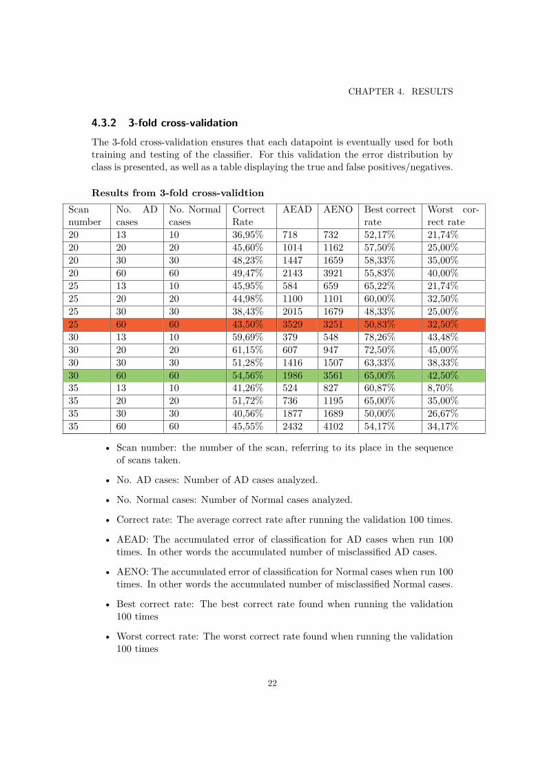
4.3.2 3-fold cross-validationThe 3-fold cross-validation ensures that each datapoint is eventually used for bothtraining and testing of the classifier. For this validation the error distribution byclass is presented, as well as a table displaying the true and false positives/negatives.

Results from 3-fold cross-validtionScannumber

No. ADcases

No. Normalcases

CorrectRate

AEAD AENO Best correctrate

Worst cor-rect rate

20 13 10 36,95% 718 732 52,17% 21,74%20 20 20 45,60% 1014 1162 57,50% 25,00%20 30 30 48,23% 1447 1659 58,33% 35,00%20 60 60 49,47% 2143 3921 55,83% 40,00%25 13 10 45,95% 584 659 65,22% 21,74%25 20 20 44,98% 1100 1101 60,00% 32,50%25 30 30 38,43% 2015 1679 48,33% 25,00%25 60 60 43,50% 3529 3251 50,83% 32,50%30 13 10 59,69% 379 548 78,26% 43,48%30 20 20 61,15% 607 947 72,50% 45,00%30 30 30 51,28% 1416 1507 63,33% 38,33%30 60 60 54,56% 1986 3561 65,00% 42,50%35 13 10 41,26% 524 827 60,87% 8,70%35 20 20 51,72% 736 1195 65,00% 35,00%35 30 30 40,56% 1877 1689 50,00% 26,67%35 60 60 45,55% 2432 4102 54,17% 34,17%

• Scan number: the number of the scan, referring to its place in the sequenceof scans taken.

• No. AD cases: Number of AD cases analyzed.

• No. Normal cases: Number of Normal cases analyzed.

• Correct rate: The average correct rate after running the validation 100 times.

• AEAD: The accumulated error of classification for AD cases when run 100times. In other words the accumulated number of misclassified AD cases.

• AENO: The accumulated error of classification for Normal cases when run 100times. In other words the accumulated number of misclassified Normal cases.

• Best correct rate: The best correct rate found when running the validation100 times

• Worst correct rate: The worst correct rate found when running the validation100 times

22

4.3. CLASSIFICATION ACCURACY

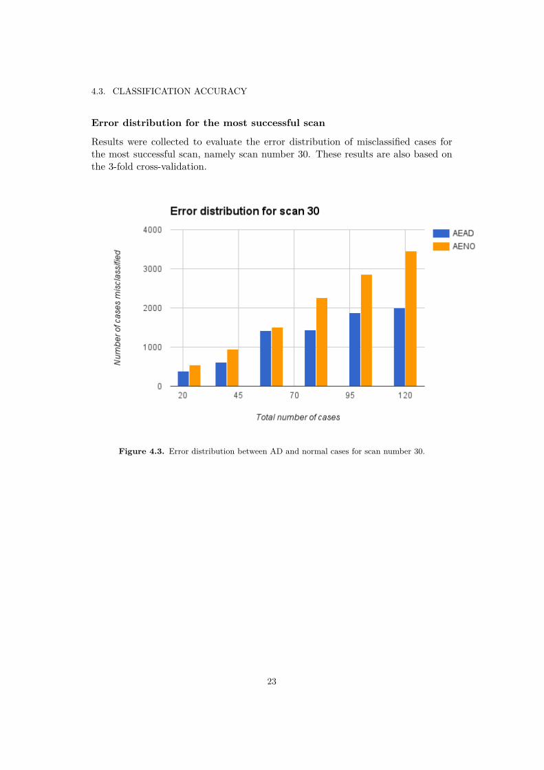
Error distribution for the most successful scan

Results were collected to evaluate the error distribution of misclassified cases forthe most successful scan, namely scan number 30. These results are also based onthe 3-fold cross-validation.

Figure 4.3. Error distribution between AD and normal cases for scan number 30.

23

Chapter 5

Discussion

The results of this study are to some extent consistent with those of Lahmiri andBoukadoum. Since the aim of the report is to apply the method developed by themin 2013 it is vital that the implementation is as consistent towards theirs as possiblefor an accurate comparison to be possible. Starting by examining the signals createdin our implementation we conclude that the signals are very similar to those pre-sented by Lahmiri and Boukadoum (2013, p. 1508). Therefore this adds credibilityto further results of this study, as the consistency between this implementation andthe one presented by Lahmiri and Boukadoum is essential. This study concludesthat the 30th scan in the sequence had the best classification accuracy when usedto perform a diagnosis. In the best case the from the 3-fold cross-validation theaccuracy was as high as 65%, which is quite good when comparing to the resultsof the CAD Dementia challenge. This scan is close to the frontal lobe, and is thusconsistent with the theory of AD originating from this area of the brain. When ex-amining the results for the large dataset it becomes apparent that no other layer ofthe brain can obtain this level of accuracy. The mean accuracy for scan number 30is 54,56%, comparing to 45,55% for scan number 35, which is the second best scanaccording to this study. These results are consistent when looking at the resultsfrom the LOOCV also. It is also noteworthy that the best accuracy obtained forthe smallest dataset with 23 cases is 78,26% from the 3-fold cross-validation, whichis a very good result, even if the mean is 59,69%. This result adds promise to theimplementation, as it is a good result, even if it cannot compare to the 100% accu-racy obtained by Lahmiri and Boukadoum for a dataset of the same size. However,if we only compare with the LOOCV results, as this is the same validation methodas used by Lahmiri and Boukadoum, the result is fairly poor as mean accuracy forscan number 30 is 55,0%. However, it is not clear if the 100% accuracy from Lahmiriand Boukadoum was the mean accuracy, although we assume it is the mean valueas stating the best accuracy obtained from a LOOCV validation would be trivial.

By regarding the error distribution by class for scan number 30 it appears asif the di�culty of distinguishing AD from normal cases becomes more prominentin the large dataset for both validation methods. In figure 4.2 and 4.3 we observe

24

5.1. DISCUSSION ON THE DATA USED

that the number of misclassified cases of normal brains increases with the size of thedataset, and that this increase is consistently greater when comparing to the numberof misclassified AD cases. For the purpose of the diagnosis it is preferred that thenumber of misclassified cases is greater for the normal cases than for the AD cases.As the system can be considered more reliable if it is more common to accidentlyclassify a normal case as AD, than actually classifying an AD case as a normalcase. Since the purpose of the system is to detect a disease that can be di�cult todiagnose by other measures, it is better to send false alarms than to let the diseasepass the system unnoticed. Future studies could address the error distribution for acorresponding scan on a larger dataset and investigate if the number of misclassifiedAD cases decreases at some point.

For both methods of validation the accuracy of the classification declined whenattempting to scale the proposed solution to a larger dataset. However, as this studywas unable to obtain the excellent level of accuracy even for the small dataset itis plausible that the implementation di�ers from that of Lahmiri and Boukadoum.Since this study failed to reproduce their results for the small dataset the resultspresented here cannot be seen as conclusive. It is possible that a small di�er-ence in the feature extraction of this study make these results inconclusive whenattempting to verifying how well the solution scales to a larger dataset. Whenconsidering other factors than the technical implementation itself this study alsoused another resource for the original data than Lahmiri and Boukadoum did. TheADNI database contains detailed information of each person who participated inthe study and by which protocol the MRI scans was collected. It is possible thatmissing details in the description of the data used in Lahmiri and Boukadoum studyled to a di�erence in the data that could account for some of the di�erences in theresult. Although, the di�culty for the classifier of this study to distinguish betweenAD and normal cases suggests that the features extracted were too similar betweenthe two classes examined.

5.1 Discussion on the data used

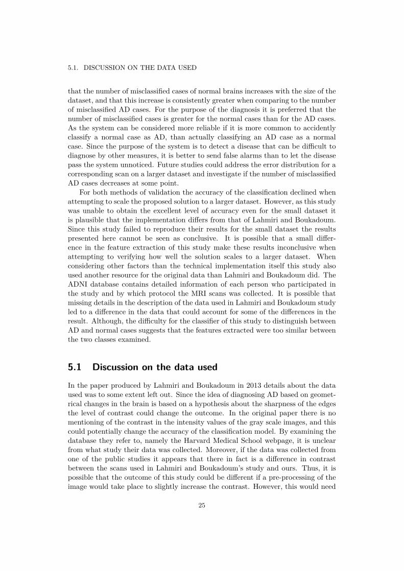
In the paper produced by Lahmiri and Boukadoum in 2013 details about the dataused was to some extent left out. Since the idea of diagnosing AD based on geomet-rical changes in the brain is based on a hypothesis about the sharpness of the edgesthe level of contrast could change the outcome. In the original paper there is nomentioning of the contrast in the intensity values of the gray scale images, and thiscould potentially change the accuracy of the classification model. By examining thedatabase they refer to, namely the Harvard Medical School webpage, it is unclearfrom what study their data was collected. Moreover, if the data was collected fromone of the public studies it appears that there in fact is a di�erence in contrastbetween the scans used in Lahmiri and Boukadoum’s study and ours. Thus, it ispossible that the outcome of this study could be di�erent if a pre-processing of theimage would take place to slightly increase the contrast. However, this would need

25

CHAPTER 5. DISCUSSION

to be evaluated in future studies before drawing any conclusions.

Figure 5.1. To the left you see scan number 30 from an AD case collected fromthe ADNI database (ADNI-database, 2006), and to the right is the approximatecorresponding scan from the Harvard Medical School database (n.d.). These imagesillustrate the di�erence in contrast between the two scans..

The dataset used here is considerably larger than that of Lahmiri and Boukadoum(2013, p. 1507), since this dataset consisted of 120 di�erent cases in total, compar-ing to the 23 cases used in 2013. The ADNI database is remarkable in its size, andthe reason that this dataset was limited to 120 cases was that we wanted to ensurethe consistency between the di�erent cases. All the cases used in this study werecollected using the same scanning protocol, however it is possible that the datasetcould be extended in future studies. Moreover, owing to the long calculation timeof the DFA it was outside the scope of this study to consider a dataset larger than200 cases. Thus, it was not considered feasible to extend the dataset during thisstudy.

5.2 Discussion on the method implementedAs the implementation of the SVMs were done using MATLAB’s standard libraryit is assumed that this part of the implementation is reliable. Also, when comparingour 1-D-signals with the ones obtained by Lahmiri and Boukadoum (2013, p.1508)they seem consistent. Thus, when considering the method one other area of uncer-tainty is whether our feature extraction was consistent with the one performed byLahmiri and Boukadoum. When implementing Hurst’s exponent we found it di�-cult to find a reliable implementation consistent with the original Hurst exponent asused by Lahmiri and Boukadoum. Therefore we instead extracted the generalizedHurst exponent, treating the data as a time series of first-order moments, since thisstudy does not consider multi-scaling properties of the data analyzed. As stated byDi Metteo, when extracting the generalized Hurst exponent for q = 1, “the value ofthis exponent is expected to be closely related to the original Hurst exponent, H,

26

5.2. DISCUSSION ON THE METHOD IMPLEMENTED

which is indeed associated with the scaling of the absolute spread in the increments”(2007, p. 25). Hence, this study relies on the similarity between the generalizedHurst and the original Hurst during the circumstances stated above.

When thoroughly examining the method as it is presented by Lahmiri andBoukadoum (2013) it becomes apparent that there are two ways of interpretinghow the MRI scans were analyzed in their study. Each case consists of a collectionof MRI scans, so the diagnosing of AD can either be done considering a whole set orjust a chosen scan. Which one of the Lahmiri and Boukadoum (2013) have chosen isnot clear. In their methods they only address the question of individual 1-D signals,and do not account for how the collected data for a brain is treated in detail. Theirpaper only shows two MRI scans of two di�erent brains, one normal and one withAD. However, the images seem to be from slightly di�erent layers, which gave riseto even more uncertainty for the implementation of this study. Yet, their method ofperforming the signal analysis is highly unlikely to have been performed on a wholebrain, but can only have been performed on one 1-D signal representing one layerof a brain. Furthermore, if one contemplates the idea of actually performing thesignal analysis on each layer of the brain to then send the resulting feature vectorsto a classifier, one quickly discovers that the results of the classification would beinconclusive. As there are many structural di�erences between layers of the brainwe believe that it would be very di�cult to train a classifier to perform a diagnosison such inconsistent data. Moreover, this would imply a massive amount of datafor the system to process, considering that for a set of 120 patients, the featureextraction would be performed 6000 times. Taking into account that the DFA takesapproximately 102 seconds to perform, computing the features for all layers of 120brains would take seven days on a 2.6 GHz Intel Core i7 processor on Mac OS X10.9.4. The time of computation is substantial and constitutes a limit on futureinvestigations.

If each layer of the brain was to be considered separately a future improvementcould be to train an ensemble of SVMs, so that there is a SVM specialized for eachlayer of the brain. Owing to the time constraint of the feature extraction a futureinvestigation could focus on a smaller region of the brain, for example by analyzingscans close to the frontal lobe. In such an approach the number of scans consideredper case could be limited to 6 or 8, and a more sophisticated system could bedeveloped to have one SVM specialized for each of the considered layers. Therebya two step classification could take place, first the individual scans are classified,and then the result for all scans belonging to a case form the basis for classificationof the case itself. This is approach would add complexity to the system, but couldprovide valuable insights to the patterns of AD in a selected region of the brain.

27

Chapter 6

Conclusion

This study fails to verify how Lahmiri and Boukadoum’s method from 2013 performson a larger dataset, as their results for a small dataset could not be reproduced in thisimplementation. However, this implementation of the method shows some promise,as the best result for the large dataset was as high as 65% using the 3-fold cross-validation. Since the proposed system does not reach a satisfactory level of accuracyfor distinguishing between cases of AD and normal cases no attempt was made atalso diagnosing MCI. However, as introduced in the discussion, future researchcould investigate how well an ensemble of SVMs could be trained to specialize indiagnosing di�erent layers of the brain. By then adding a second classificationthe collected diagnoses of the layers could form the basis for diagnosing the caseas a whole. Future implementations could also consider if small enhancementsof contrast in the original MRI scans can improve the classification accuracy byslightly increasing the geometrical di�erences of the original images prior to thefeature extraction.

28

Chapter 7

References

ADNI-database, 2006 [online]. Available at: <https://ida.loni.usc.edu/login.

jsp>[Accessed date 16th April 2015]

alz.org . AD progressing in a brain [image online]Available at: <http://www.alz.org/alzheimers_disease_what_is_alzheimers.

asp>[Accessed 25 March 2015].

alz.org, n.d. [online] Brain Imaging.Available at: <http://www.alz.org/alzheimers_disease_steps_to_diagnosis.

asp#brain>[Accessed 25 March 2015]

alz.org, n.d. Diagnosis of Alzheimer’s and Dementia [online].Available at: <http://www.alz.org/alzheimers_disease_diagnosis.asp>[Accessed 25 March 2015]

Aquilonius S.M, 2009. Alzheimers sjukdom. [online] Nationalecyklopedin.Avaialble at: <http://www.ne.se/uppslagsverk/encyklopedi/l�ng/alzheimers-sjukdom>[Accessed 25 March 2015]

Aston, T, 2013. Generalized Hurst exponent [online]. Available at: <http://www.

mathworks.com/matlabcentral/fileexchange/30076-generalized-hurst-exponent>[Accessed 25 March 2015]

Bron E.E et al, 2015. Standardized evaluation of algorithms for computer-aideddiagnosis of dementia based on structural MRI: The CADDementia challenge,NeuroImage, Volume 111, p. 562–579.

29

CHAPTER 7. REFERENCES

Byvatov, E., Schneider, G., 2003. Support vector machine applications inbioinformatics. Applied Bioinformatics, Volume 2, p. 67-77.

Gustafson L, 2009. Demens [online] Nationalecyklopedin.Avaialble at: <http://www.ne.se/uppslagsverk/encyklopedi/l�ng/demens>[Accessed 25 March 2015]

Harvard Medical School Database, n.d [online]. Available at: <http://www.med.

harvard.edu/AANLIB/cases/case29/mr1-tc1/014.html>[Accessed 28 April 2015

[Home] AIBL. Available at: <http://aibl.csiro.au/about/organisation/>

Kale M, Butar Butar F, 2015. Fractal Analysis of Time Series and DistributionProperties of Hurst Exponent. Available through: <http://msme.us/2011-1-2.

pdf>[Accessed 6 May 2015]

Lahmiri, S. and Boukadoum, M., 2011. Brain MRI Classification using an EnsembleSystem and LH and HL Wavelet Sub-bands Features. Computational IntelligenceIn Medical Imaging (CIMI), 2011 IEEE Third International Workshop On.Paris, 11-15 April 2011.

Lahmiri, S. and Boukadoum, M., 2012. Automatic Brain MR Images DiagnosisBased on Edge Fractal Dimension and Spectral Energy Signature. 34th AnnualInternational Conference of the IEEE EMBS.San Diego, California USA, 28 August - 1 September, 2012.

Lahmiri, S. and Boukadoum, M, 2013. Automatic Detection of Alzheimer Diseasein Brain Magnetic Resonance Images Using Fractal Features. 6th Annual Interna-tional IEEE EMBS Conference on Neural Engineering.San Diego, California, 6 - 8 November, 2013.

Lahmiri, S. and Boukadoum, M, 2014. New approach for automatic classificationof Alzheimer’s disease, mild cognitive impairment and healthy brain magnetic res-onance images. Healthcare Technology Letters, 2014, Vol. 1, Iss. 1, p. 32–36.

Malmquist J, n.d. Mild Kognitiv Svikt. [online] Nationalencyklopedin.Avaialble at: <http://www.ne.se/uppslagsverk/encyklopedi/l�ng/mild-kognitiv-svikt>[Accessed 20 April 2015]

Matteo, T. Di, 2007. Multi-scaling in finance, Quantitative Finance,Volume 7, No. 1, p. 21–36.

30

Medicinenet, 2015. Alzheimer’s Disease Causes, Stages, and Symptoms. [online]Available at:<http://www.medicinenet.com/alzheimers_disease_causes_stages_

and_symptoms/page3.htm#what_are_the_symptoms_of_alzheimers_disease>[Accessed 25 March 2015]

Peng, C.-K., Buldyrev, S.V., Havlin, S., Simons, M., Stanley, H. E., and Goldberger,A. L., 1994. Mosaic organization of DNA nucleotides.Physical Review E, Volume 49, page 1685.

Physionet.org , n.d. Detrended Fluctuation Analysis [online]Avaialble at: <http://physionet.org/physiotools/dfa/>[Accessed 25 March 2015]

Schneider J, 1997. Cross Validation [online]. Available at: Carnegie Mellon Univer-sity. <http://www.cs.cmu.edu/~schneide/tut5/node42.html>[Accessed 29 april 2015]

WebMD, 2012. Magnetic Resonance Imaging (MRI) of the Head, [online].Available at: <http://www.webmd.com/brain/magnetic-resonance-imaging-mri-of-the-head>[Accessed 25 March 2015]

Weston J , n.d. Support Vector Machine (and Statistical Learning Theory) Tutorial[online] columbia.edu.Avaialble at: <http://www.cs.columbia.edu/~kathy/cs4701/documents/jason_

svm_tutorial.pdf>[Accessed 26 March 2015]

31

www.kth.se