EU-PEMS PM EVALUATION PROGRAM - Third Report – Further ...publications.jrc.ec.europa.eu/repository/bitstream/JRC65948/lb-na-24883-en-c.pdf · EU-PEMS PM EVALUATION PROGRAM - Third

EUR 24883 EN - 2011

EU-PEMS PM EVALUATION PROGRAM - Third Report – Further Study on Post DPF

PM/PN Emissions

A. Mamakos, M. Carriero, P. Bonnel,

H. Demircioglu, K. Douglas

S. Alessandrini, F. Forni, F. Montigny, D. Lesueur

The mission of the JRC-IE is to provide support to Community policies related to both nuclear and non-nuclear energy in order to ensure sustainable, secure and efficient energy production, distribution and use. European Commission Joint Research Centre Institute for Energy Contact information Pierre Bonnel, Massimo Carriero Address: Joint Research Center, Via Enrico Fermi 2749, 21027 Ispra (VA), Italy E-mail: [email protected], [email protected] Tel.: +39 0332 785301, +39 0332 786354 Fax: +39 0332 785236 http://ies.jrc.ec.europa.eu/ http://www.jrc.ec.europa.eu/ Legal Notice Neither the European Commission nor any person acting on behalf of the Commission is responsible for the use which might be made of this publication. Europe Direct is a service to help you find answers to your questions about the European Union Freephone number (*): 00 800 6 7 8 9 10 11 (*) Certain mobile telephone operators do not allow access to 00 800 numbers or these calls may be billed. A great deal of additional information on the European Union is available on the Internet. It can be accessed through the Europa server http://europa.eu/ JRC 65948 EUR 65948 EN ISBN 978-92-79-20695-5 (print) ISBN 978-92-79-20696-2 (online) ISSN 1018-5593 (print) ISSN 1831-9424 (online) doi:10.2788/34166 (print) Luxembourg: Publications Office of the European Union © European Union, 2011 Reproduction is authorised provided the source is acknowledged Printed in Italy

TABLE OF CONTENTS

1 INTRODUCTION ................................................................................................................7

1.1 BACKGROUND ............................................................................................................7

1.2 PREVIOUS FINDINGS AND OUTLINE OF THE PRESENT WORK...........................7

2 Experimental .....................................................................................................................10

2.1 CANDIDATE INSTRUMENTS....................................................................................10

2.1.1 HORIBA’s OBS ..................................................................................................10

2.1.2 AVL PM PEMS 494............................................................................................11

2.1.3 Control Sistem’s m-PSS.....................................................................................12

2.1.4 Sensors PPMD...................................................................................................13

2.1.5 DMM...................................................................................................................14

2.2 Experimental facilities .................................................................................................14

2.2.1 Test Engine ........................................................................................................14

2.2.2 Fuel and Lubricating Oil .....................................................................................15

2.2.3 Reference Sampling Instrumentation.................................................................17

2.2.4 Reference Aerosol Instrumentation ...................................................................18

2.2.5 Aerosol Generators ............................................................................................21

2.3 GENERAL OUTLINE OF THE EXPERIMENTAL SETUP .........................................23

2.3.1 Engine Testing ...................................................................................................23

2.3.2 Calibration Experiments .....................................................................................25

2.4 Test procedures..........................................................................................................27

3 Experimental results .........................................................................................................29

3.1 Reference laboratory instrumentation ........................................................................29

3.1.1 PM emissions .....................................................................................................29

3.1.2 Solid particle number emissions ........................................................................34

3.1.3 Size distributions ................................................................................................36

3.1.4 Effective particle density ....................................................................................36

3.1.5 Real time airborne non-volatile particle mass....................................................40

3.2 PPMD..........................................................................................................................42

3.2.1 Modifications ......................................................................................................42

3.2.2 Correlation of CQCM mass to PM and total carbon ..........................................42

3.2.3 Crystal to crystal variability.................................................................................44

3.2.4 Possibility to use of CQCM signal as real time sensor ......................................45

3.2.5 Effect of relative humidity ...................................................................................47

3.3 MSS and GFB.............................................................................................................49

3.3.1 Modifications ......................................................................................................49

3.3.2 GFB results ........................................................................................................49

3.3.3 MSS results ........................................................................................................50

3.4 DMM ...........................................................................................................................57

3.4.1 Modifications ......................................................................................................57

3.4.2 Correlation with EC and mass of airborne “non-volatile” particles.....................57

3.4.3 Number results ...................................................................................................59

3.4.4 Real time responses...........................................................................................60

3.5 OBS ............................................................................................................................62

3.5.1 Modifications ......................................................................................................62

3.5.2 PM results ..........................................................................................................62

3.5.3 DCS calibration ..................................................................................................63

3.5.4 DCS responses to engine exhaust ....................................................................64

3.6 m-PSS.........................................................................................................................67

3.6.1 Modifications ......................................................................................................67

3.6.2 PM results ..........................................................................................................67

3.6.3 PPS calibration...................................................................................................68

3.6.4 PPS response to diesel engine exhaust ............................................................72

4 Conclusions ......................................................................................................................76

4.1 Effect of sampling time on PM emissions...................................................................76

4.2 COMPARABILITY OF THE GRAVIMETRIC PM EMISSIONS MEASUREMENT METHODS............................................................................................................................76

4.3 NON-VOLATILE PM ...................................................................................................76

4.4 PPMD..........................................................................................................................76

4.5 MSS & GFB ................................................................................................................77

4.6 DMM ...........................................................................................................................77

4.7 OBS ............................................................................................................................78

4.8 m-PSS.........................................................................................................................78

5 LIST OF SPECIAL TERMS AND ABBREVIATIONS .......................................................79

6 REFERENCES .................................................................................................................81

ACKNOWLEDGMENTS

The present work was conducted in co-operation with the experts of the companies as listed below. The European Commission expresses its gratefulness for their co-operation and the provision of the equipment used during this program.

MM. Les Hill, Daniel Scheder (HORIBA)

M. Cesare Bassoli, Daniele Testa (CONTROL SISTEM)

MM. Oliver Franken, Lauretta Rubino, David Booker (SENSORS EUROPE, SENSORS INC)

MM. Karl Obergugenberger, Wolfgang Schindler (AVL)

MM. Ville Niemela, Erkki Lamminen (DEKATI)

1 INTRODUCTION

1.1 BACKGROUND The present work was conducted in the frame of the EU-PEMS PM evaluation programme. The program was launched in 2008 by the European Commission to assess the potential of portable instruments to measure particulate emissions on-board of vehicles. The EU-PEMS program is a voluntary program, receiving contributions from the European Joint Research Center (JRC), some portable emissions equipment manufacturers (AVL, Dekati, Control Sistem, Horiba, Sensors Inc.) and the European association of heavy-duty engines manufacturers (ACEA).

The text of the call underlined the objectives of the program and defined the list of the basic technical requirements to be met by the instruments to be valid candidates.

The candidate instruments had to fulfil a few basic requirements:

• To measure the total Particulate Matter (PM) mass over a long sampling period, either following the standard method or using a method proven to be equivalent to the standard method;

• To provide a second-by second (“real-time”) information on the emitted PM mass at any time during the test. This is a necessary pre-requisite for evaluating the data according to the Moving Average Window (MAW) method (work or CO2 based);

• To be ready for on-vehicle tests and in particular to include a solution to transport the raw or the diluted exhaust, to allow for an installation of the system within a few meters from the vehicle tailpipe.

Measurement principles that were not fully in line with the laboratory standard methods to measure PM mass were also accepted for evaluation, either with variations of the dilution method (e.g. constant dilution) or with alternative physical principles (e.g. measurement of the soot instead of total PM).

Upon the conclusions of the study, the main conclusions of the project were to recommend the candidate principle(s) and to discuss whether the corresponding technological progress of the instruments was sufficient to foresee a short term introduction in the legislation.

1.2 PREVIOUS FINDINGS AND OUTLINE OF THE PRESENT WORK The figure below shows the different phases of the program, spread between 2009 and 2010 and how each phase of the evaluation has addressed different topics. The first phase main objective focused on the identification of instrumentation principles. Five in total candidate systems were evaluated on the Heavy Duty Engine (HDE) test bench of the Vehicle Emissions LAboratories (VELA) of the JRC, using the exhaust of three HDEs. These included a 10 l Cursor Euro III engine equipped with an EMITEC Partial Flow Deep Bed Filter, a 10 l Man Euro V engine equipped with a Selective Catalytic Reduction (SCR) after-treatment system and a 15 l Cummins US07 engine equipped with an active regeneration Diesel Particulate Filter (DPF).

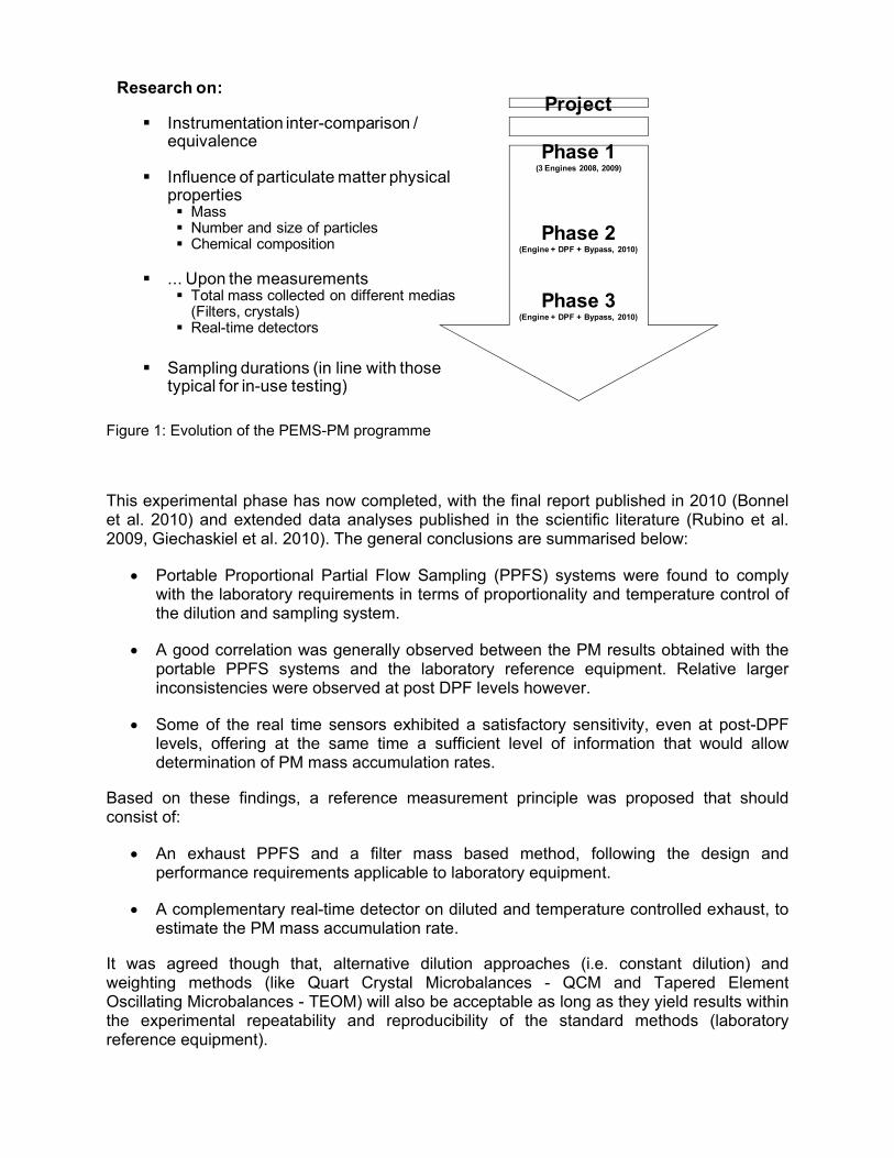
Research on:

Instrumentation inter-comparison / equivalence

Influence of particulate matter physical properties

MassNumber and size of particlesChemical composition

... Upon the measurementsTotal mass collected on different medias (Filters, crystals)Real-time detectors

Sampling durations (in line with those typical for in-use testing)

Project

Phase 1(3 Engines 2008, 2009)

Phase 2(Engine + DPF + Bypass, 2010)

Phase 3(Engine + DPF + Bypass, 2010)

Figure 1: Evolution of the PEMS-PM programme

This experimental phase has now completed, with the final report published in 2010 (Bonnel et al. 2010) and extended data analyses published in the scientific literature (Rubino et al. 2009, Giechaskiel et al. 2010). The general conclusions are summarised below:

• Portable Proportional Partial Flow Sampling (PPFS) systems were found to comply with the laboratory requirements in terms of proportionality and temperature control of the dilution and sampling system.

• A good correlation was generally observed between the PM results obtained with the portable PPFS systems and the laboratory reference equipment. Relative larger inconsistencies were observed at post DPF levels however.

• Some of the real time sensors exhibited a satisfactory sensitivity, even at post-DPF levels, offering at the same time a sufficient level of information that would allow determination of PM mass accumulation rates.

Based on these findings, a reference measurement principle was proposed that should consist of:

• An exhaust PPFS and a filter mass based method, following the design and performance requirements applicable to laboratory equipment.

• A complementary real-time detector on diluted and temperature controlled exhaust, to estimate the PM mass accumulation rate.

It was agreed though that, alternative dilution approaches (i.e. constant dilution) and weighting methods (like Quart Crystal Microbalances - QCM and Tapered Element Oscillating Microbalances - TEOM) will also be acceptable as long as they yield results within the experimental repeatability and reproducibility of the standard methods (laboratory reference equipment).

However the study also identified some open issues that required additional investigation. The major concern was the observed deterioration in the correlation between the PM results of the portable and the reference systems at current PM levels and below. At these emission levels, some inconsistencies were also observed in the responses of the different real time sensors.

In an attempt to address these issues and better understand the properties of PM at such low emission levels, a follow-up activity was undertaken. Two diesel HDEs were employed in with a CRT / Bypass configuration that allowed an adjustment of the emission levels from Euro V (20 mg/km) to CRT out. The study was carried out in two phases (Phase 2 and Phase 3).

Phase 2 focused on the contribution of background and adsorbed material on PM. To this end, the PM emissions at four in total different levels were quantified using Teflon, TX40 and Quartz filters. The latter provided the means to quantify the Elemental Carbon (EC) content of PM. Calibrated reference aerosol instrumentation was also employed in parallel and the collected data analyzed to estimate the mass of airborne particles in real time. This served as an additional benchmark (complimentary to EC and PM) against which the different real time sensors were evaluated. The study also investigated cross-sensitivities of the different sensors to non-PM sources (like humidity and other gaseous pollutants). The results of these investigations have already been published (Mamakos et al. 2011).

In response to the findings of the second experimental phase, some of the instrument manufacturers undertook some remedy measures. The modified instrumentation was then evaluated in the third phase which also investigated the consistency of the PM results with respect to the sampling time. The results of these investigations are summarized in the present report.

2 EXPERIMENTAL

2.1 CANDIDATE INSTRUMENTS Five in total candidate PEMS-PM systems were employed in this study, namely:

• Micro Particulate Sampling System (m-PSS) by Control Sistem

• Micro Soot Sensor (MSS) with Gravimetric Filter Box (GFB) by AVL

• Dekati Mass Monitor (DMM)

• On Board System with Transient Response Particulate Measurement unit (OBS-TRPM, abbreviated as OBS hereinafter) by Horiba

• Portable Particle Measurement Device (PPMD) by Sensors

Some of the instruments were modified to remedy some issues revealed in the second phase of the project (Mamakos et al. 2011). In particular:

• The filter holder of the AVL GFB was modified to reduce the stain area of the filter, through the use of a spacer that was employed when TX40 filters were used.

• The quartz crystals of the Carousel Quartz Crystal Microbalance (CQCM) of the PPMD were replaced with new ones provided by Sensors.

• Control Sistem replaced the Pegasor Particle Sensor (PPS) of the m-PSS with a latter version prototype.

• The Diffusion Charge Sensor (DCS) of the OBS was received after the necessary maintenance at TSI.

The five candidate systems are described briefly in the following sections.

2.1.1 HORIBA’s OBS

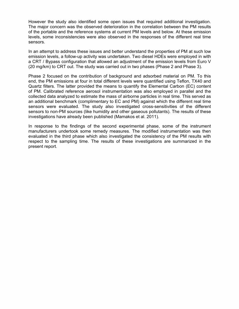
Horiba’s OBS is an ob-board proportional partial flow system that collects mass on 47 mm filters at a total flowrate of 30 lpm (Wei et al. 2009). A schematic of the OBS is given in Figure 2. Dilution takes place at the sampling probe where the sample is drawn at a flowrate proportional to the exhaust flow. The diluted exhaust is then transported to the filter cabinet with a 4 m heated (at 47°C) line. The cabinet, which also incorporates a cyclone to remove large particles (cut point at 6 um), is also maintained at a temperature of 47°C by means of direct surface heating.

A small amount of the diluted exhaust is bypassed to a TSI’s Diffusion Charge Sensor (DCS), which is a modified version of the Electrical Aerosol Detector (EAD), measuring the total particle length in real time (Frank et al. 2008). The operation principle of the DCS is based on diffusion charging of the aerosol, followed by detection of the charged particles via a sensitive electrometer. Part of the sampled flow (1 lpm from the total 2.5 lpm) is passing through an absolute filter and then through a corona charger producing the air ions. This flow of ions is reunited with the remaining air flow in a mixing chamber bringing particles into a well defined charge state. The charged aerosol then passes through an ion trap that removes any excess

ions before being detected in the electrometer. The number of elementary units of charge acquired in this counter flow diffusion charger is found to be linearly related to the diameter of the particles. Therefore the total current measured in the electrometer is proportional to the total length of the sampled aerosol.

Figure 2: Horiba’s OBS: Schematic of its principle of operation

2.1.2 AVL PM PEMS 494

The system from AVL utilizes a constant dilution partial flow system sampling exhaust at a constant flowrate. The dilution system, referred to as AVL’s conditioning unit, allows for a dilution of up to 12 and a temperature and pressure conditioning of the diluted exhaust (temperature below 60°C and pressure at ambient ±50 mbar). The exhaust gas is diluted with a dilution cell which was mounted directly at the sample point to minimize particle losses. The diluted exhaust gas is sampled in parallel through the MSS measuring cell and over the measurement filter inside the GFB. Therefore one heated line which is connected to the GFB box is used. The MSS and GFB box is connected via an insulated hose. The flowrates are 2 lpm for the MSS and 5 lpm for the GFB. The GFB is externally heated by direct surface heating to control the filter face temperature to 47°C (±5°C). This prototype GFB did not incorporate a cyclone.

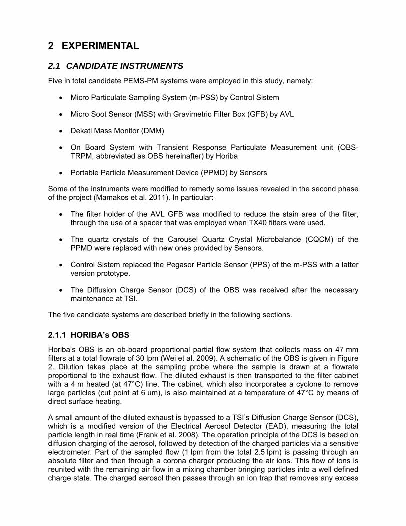
The MSS operates on the photoacoustic principle (Schindler et al. 2004). The exhaust aerosol passes through a resonator cell were it is exposed to an intensity modulated 808 nm laser beam. This “chopped” light beam is absorbed by the soot particles leading in a periodic heating and cooling of the air surrounding the particles (Figure 3). This is manifested as a periodic pressure wave which is measured by a sensitive microphone and the signal amplified in a “lock-in” amplifier. The 808 nm wavelength was selected in order to minimize interferences from other exhaust gas components and any volatile compounds of PM. Therefore, the microphone signal is proportional to the mass of soot particles.

(a)

(b)

Figure 3: AVL 483 MSS (a) and a schematic of its principle of operation (b)

2.1.3 Control Sistem’s m-PSS

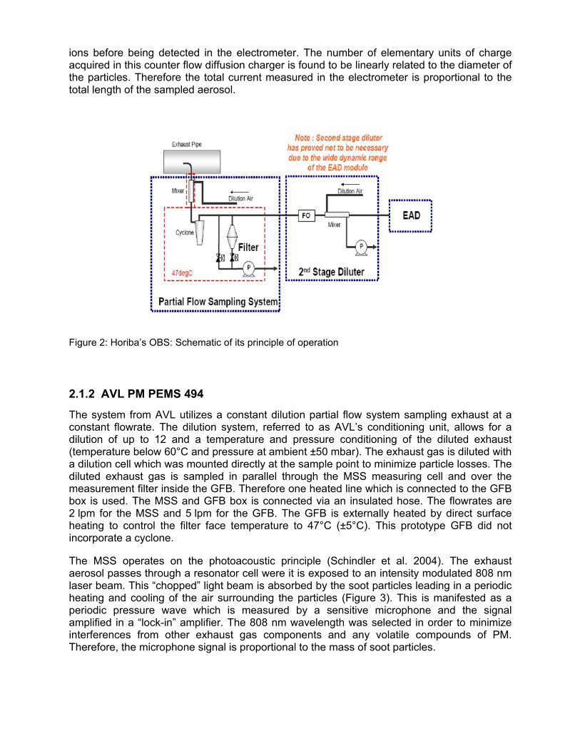
The Micro Particulate Sampling Sistem (m-PSS) (Control Sistem) is as a proportional partial flow system (the on-board version of PSS-20) that does not require compressed air or cooled water. PM samples are collected on 47 mm filters at a flowrate of 30 lpm. The filter temperature is kept at 47±5°C by means of heating the dilution air. The system does not incorporate a cyclone.

The particular unit was equipped with a prototype particle sensor developed by Pegasor Ltd. The operation principle of the Pegasor Particle Sensor (PSS) is based on the electrostatic charging of particles and the subsequent measurement of current induced as the charged aerosol passes through the sensor. This flow through design does not require collection of particles for the measurement of their charge and therefore the extracted flow is returned in the m-PSS at a point upstream of the filter. The PSS also incorporates an ejector diluter to protect the corona needle from getting contaminated. The necessary pressurised dilution air was provided by a pump located in the m-PSS. This additional dilution air was taken into account for the control of the total diluted flowrate.

(a)

(b)

Figure 4: Control Sistem’s m-PSS (a) and Pegasor’s Particle Sensor (b).

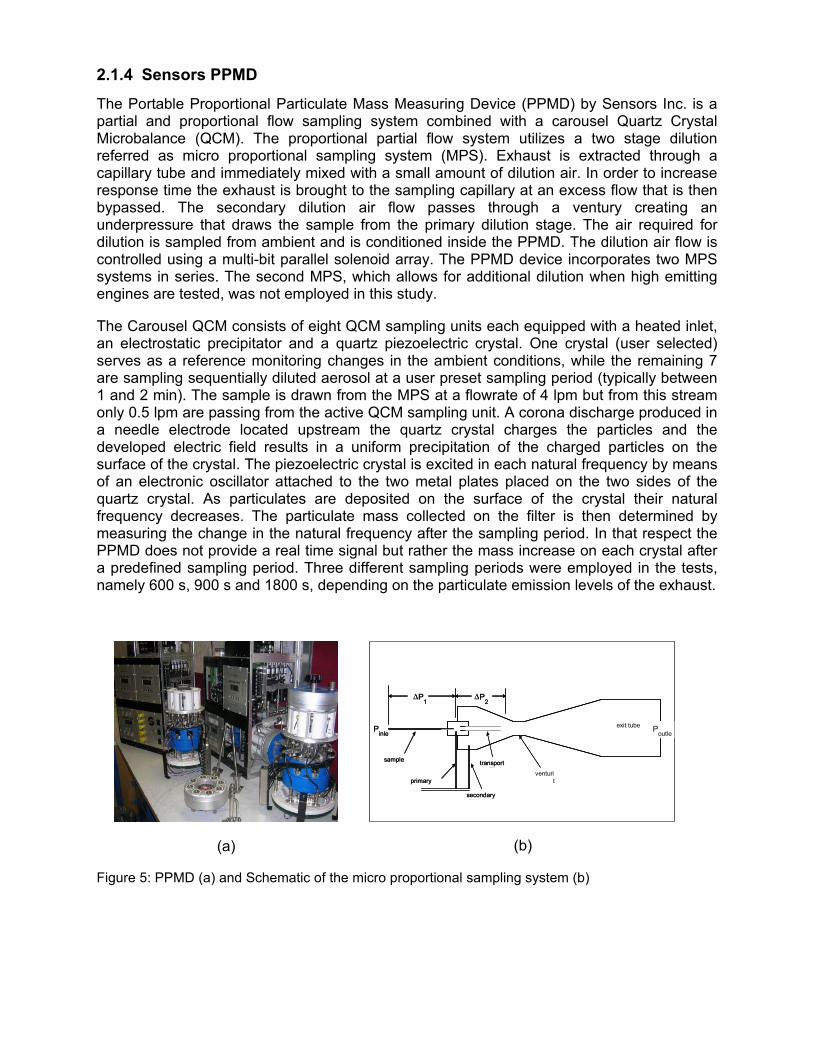
2.1.4 Sensors PPMD

The Portable Proportional Particulate Mass Measuring Device (PPMD) by Sensors Inc. is a partial and proportional flow sampling system combined with a carousel Quartz Crystal Microbalance (QCM). The proportional partial flow system utilizes a two stage dilution referred as micro proportional sampling system (MPS). Exhaust is extracted through a capillary tube and immediately mixed with a small amount of dilution air. In order to increase response time the exhaust is brought to the sampling capillary at an excess flow that is then bypassed. The secondary dilution air flow passes through a ventury creating an underpressure that draws the sample from the primary dilution stage. The air required for dilution is sampled from ambient and is conditioned inside the PPMD. The dilution air flow is controlled using a multi-bit parallel solenoid array. The PPMD device incorporates two MPS systems in series. The second MPS, which allows for additional dilution when high emitting engines are tested, was not employed in this study.

The Carousel QCM consists of eight QCM sampling units each equipped with a heated inlet, an electrostatic precipitator and a quartz piezoelectric crystal. One crystal (user selected) serves as a reference monitoring changes in the ambient conditions, while the remaining 7 are sampling sequentially diluted aerosol at a user preset sampling period (typically between 1 and 2 min). The sample is drawn from the MPS at a flowrate of 4 lpm but from this stream only 0.5 lpm are passing from the active QCM sampling unit. A corona discharge produced in a needle electrode located upstream the quartz crystal charges the particles and the developed electric field results in a uniform precipitation of the charged particles on the surface of the crystal. The piezoelectric crystal is excited in each natural frequency by means of an electronic oscillator attached to the two metal plates placed on the two sides of the quartz crystal. As particulates are deposited on the surface of the crystal their natural frequency decreases. The particulate mass collected on the filter is then determined by measuring the change in the natural frequency after the sampling period. In that respect the PPMD does not provide a real time signal but rather the mass increase on each crystal after a predefined sampling period. Three different sampling periods were employed in the tests, namely 600 s, 900 s and 1800 s, depending on the particulate emission levels of the exhaust.

(a)

ΔP1

ΔP2

transport ill

sample ill

primary dil ti

ventui

throat

Pinlet

secondary dil ti

Poutlet

ΔP1

ΔP2

transport ill

sample ill

primary dil ti

venturi th t

Pinlet

secondary dil ti

Poutlet

exit tube

(b)

Figure 5: PPMD (a) and Schematic of the micro proportional sampling system (b)

2.1.5 DMM

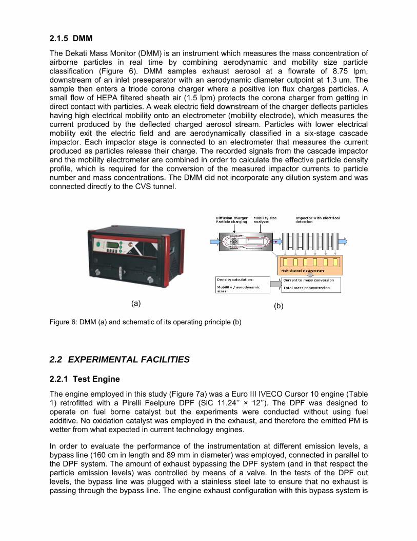
The Dekati Mass Monitor (DMM) is an instrument which measures the mass concentration of airborne particles in real time by combining aerodynamic and mobility size particle classification (Figure 6). DMM samples exhaust aerosol at a flowrate of 8.75 lpm, downstream of an inlet preseparator with an aerodynamic diameter cutpoint at 1.3 um. The sample then enters a triode corona charger where a positive ion flux charges particles. A small flow of HEPA filtered sheath air (1.5 lpm) protects the corona charger from getting in direct contact with particles. A weak electric field downstream of the charger deflects particles having high electrical mobility onto an electrometer (mobility electrode), which measures the current produced by the deflected charged aerosol stream. Particles with lower electrical mobility exit the electric field and are aerodynamically classified in a six-stage cascade impactor. Each impactor stage is connected to an electrometer that measures the current produced as particles release their charge. The recorded signals from the cascade impactor and the mobility electrometer are combined in order to calculate the effective particle density profile, which is required for the conversion of the measured impactor currents to particle number and mass concentrations. The DMM did not incorporate any dilution system and was connected directly to the CVS tunnel.

(a) (b)

Figure 6: DMM (a) and schematic of its operating principle (b)

2.2 EXPERIMENTAL FACILITIES

2.2.1 Test Engine

The engine employed in this study (Figure 7a) was a Euro III IVECO Cursor 10 engine (Table 1) retrofitted with a Pirelli Feelpure DPF (SiC 11.24’’ × 12’’). The DPF was designed to operate on fuel borne catalyst but the experiments were conducted without using fuel additive. No oxidation catalyst was employed in the exhaust, and therefore the emitted PM is wetter from what expected in current technology engines.

In order to evaluate the performance of the instrumentation at different emission levels, a bypass line (160 cm in length and 89 mm in diameter) was employed, connected in parallel to the DPF system. The amount of exhaust bypassing the DPF system (and in that respect the particle emission levels) was controlled by means of a valve. In the tests of the DPF out levels, the bypass line was plugged with a stainless steel late to ensure that no exhaust is passing through the bypass line. The engine exhaust configuration with this bypass system is

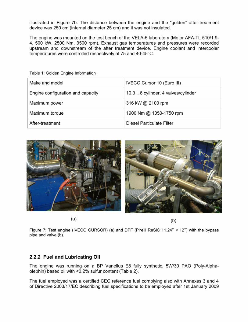
illustrated in Figure 7b. The distance between the engine and the “golden” after-treatment device was 250 cm (internal diameter 25 cm) and it was not insulated.

The engine was mounted on the test bench of the VELA-5 laboratory (Motor AFA-TL 510/1.9-4, 500 kW, 2500 Nm, 3500 rpm). Exhaust gas temperatures and pressures were recorded upstream and downstream of the after treatment device. Engine coolant and intercooler temperatures were controlled respectively at 75 and 40-45°C.

Table 1: Golden Engine Information

Make and model IVECO Cursor 10 (Euro III)

Engine configuration and capacity 10.3 l, 6 cylinder, 4 valves/cylinder

Maximum power 316 kW @ 2100 rpm

Maximum torque 1900 Nm @ 1050-1750 rpm

After-treatment Diesel Particulate Filter

(a) (b)

Figure 7: Test engine (IVECO CURSOR) (a) and DPF (Pirelli ReSiC 11.24’’ × 12’’) with the bypass pipe and valve (b).

2.2.2 Fuel and Lubricating Oil

The engine was running on a BP Vanellus E8 fully synthetic, 5W/30 PAO (Poly-Alpha-olephin) based oil with <0.2% sulfur content (Table 2).

The fuel employed was a certified CEC reference fuel complying also with Annexes 3 and 4 of Directive 2003/17/EC describing fuel specifications to be employed after 1st January 2009

(i.e. sulphur content of lower than 10 ppm). The most important properties can be seen in Table 3 and the detailed specifications in Annex A.

Table 2: Lubricating oil specifications.

Properties Method Units Value

Density @15 oC ASTM D4052 g/ml 0.860

Cinematic Viscosity @100 oC ASTM D445 mm2/s 12.03

Viscosity Index ASTM D2270 o 163

Viscosity CCS @ -30 oC ASTM D2602 cP 5260

Total Base Number ASTM D2896 Mg KOH/g 15.9

Sulphated Ash ASTM D874 oC 1.9

Specifications:

SAE 5W-30

ACEA E4/E5/E7 RVI RXD

MB approval 228.5 Cummins CES 20072/77

MAN M3277 MTU Type 3

Volvo VDS-2 Mack EO-M Plus

Scania LDF DAF HP1/HP2

Table 3:Fuel specifications.

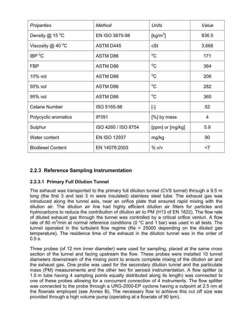
Properties Method Units Value

Density @ 15 oC EN ISO 3675-98 [kg/m3] 836.5

Viscosity @ 40 oC ASTM D445 cSt 3.666

IBP oC ASTM D86 oC 171

FBP ASTM D86 oC 364

10% vol ASTM D86 oC 208



Cetane Number ISO 5165-98 [-] 52

Polycyclic aromatics IP391 [%] by mass 4

Sulphur ISO 4260 / ISO 8754 [ppm] or [mg/kg] 5.9

Water content EN ISO 12937 mg/kg 90

Biodiesel Content EN 14078:2003 % v/v <7

2.2.3 Reference Sampling Instrumentation

2.2.3.1 Primary Full Dilution Tunnel

The exhaust was transported to the primary full dilution tunnel (CVS tunnel) through a 9.5 m long (the first 3 and last 3 m were insulated) stainless steel tube. The exhaust gas was introduced along the tunnel axis, near an orifice plate that ensured rapid mixing with the dilution air. The dilution air line had highly efficient dilution air filters for particles and hydrocarbons to reduce the contribution of dilution air to PM (H13 of EN 1822). The flow rate of diluted exhaust gas through the tunnel was controlled by a critical orifice venturi. A flow rate of 80 m3/min at normal reference conditions (0 °C and 1 bar) was used in all tests. The tunnel operated in the turbulent flow regime (Re = 25000 depending on the diluted gas temperature). The residence time of the exhaust in the dilution tunnel was in the order of 0.5 s.

Three probes (of 12 mm inner diameter) were used for sampling, placed at the same cross section of the tunnel and facing upstream the flow. These probes were installed 10 tunnel diameters downstream of the mixing point to ensure complete mixing of the dilution air and the exhaust gas. One probe was used for the secondary dilution tunnel and the particulate mass (PM) measurements and the other two for aerosol instrumentation. A flow splitter (a 1.5 m tube having 4 sampling points equally distributed along its length) was connected to one of these probes allowing for a concurrent connection of 4 instruments. The flow splitter was connected to the probe through a URG-2000-EP cyclone having a cutpoint at 2.5 nm at the flowrate employed (see Annex B). The necessary flow to achieve this cut off size was provided through a high volume pump (operating at a flowrate of 90 lpm).

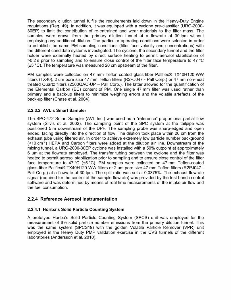
The secondary dilution tunnel fulfils the requirements laid down in the Heavy-Duty Engine regulations (Reg. 49). In addition, it was equipped with a cyclone pre-classifier (URG-2000-30EP) to limit the contribution of re-entrained and wear materials to the filter mass. The samples were drawn from the primary dilution tunnel at a flowrate of 30 lpm without employing any additional dilution. The particular operating conditions were selected in order to establish the same PM sampling conditions (filter face velocity and concentrations) with the different candidate systems investigated. The cyclone, the secondary tunnel and the filter holder were externally heated by direct surface heating to permit aerosol stabilization of >0.2 s prior to sampling and to ensure close control of the filter face temperature to 47 °C (±5 °C). The temperature was measured 20 cm upstream of the filter.

PM samples were collected on 47 mm Teflon-coated glass-fiber Pallflex® TX40H120-WW filters (TX40), 2 um pore size 47 mm Teflon filters (R2PJ047 - Pall Corp.) or 47 nm non-heat treated Quartz filters (2500QAO-UP – Pall Corp.). The latter allowed for the quantification of the Elemental Carbon (EC) content of PM. One single 47 mm filter was used rather than primary and a back-up filters to minimize weighing errors and the volatile artefacts of the back-up filter (Chase et al. 2004).

2.2.3.2 AVL’s Smart Sampler

The SPC-472 Smart Sampler (AVL Inc.) was used as a “reference” proportional partial flow system (Silvis et al. 2002). The sampling point of the SPC system at the tailpipe was positioned 5 m downstream of the DPF. The sampling probe was sharp-edged and open ended, facing directly into the direction of flow. The dilution took place within 20 cm from the exhaust tube using filtered air. In order to achieve extremely low particle number background (<10 cm-3) HEPA and Carbon filters were added at the dilution air line. Downstream of the mixing tunnel, a URG-2000-30EP cyclone was installed with a 50% cutpoint at approximately 6 μm at the flowrate employed. The transfer tubing between the cyclone and the filter was heated to permit aerosol stabilization prior to sampling and to ensure close control of the filter face temperature to 47 °C (±5 °C). PM samples were collected on 47 mm Teflon-coated glass-fiber Pallflex® TX40H120-WW filters or 2 um pore size 47 mm Teflon filters (R2PJ047 - Pall Corp.) at a flowrate of 30 lpm. The split ratio was set at 0.0375%. The exhaust flowrate signal (required for the control of the sample flowrate) was provided by the test bench control software and was determined by means of real time measurements of the intake air flow and the fuel consumption.

2.2.4 Reference Aerosol Instrumentation

2.2.4.1 Horiba’s Solid Particle Counting System

A prototype Horiba’s Solid Particle Counting System (SPCS) unit was employed for the measurement of the solid particle number emissions from the primary dilution tunnel. This was the same system (SPCS19) with the golden Volatile Particle Remover (VPR) unit employed in the Heavy Duty PMP validation exercise in the CVS tunnels of the different laboratories (Andersson et al. 2010).

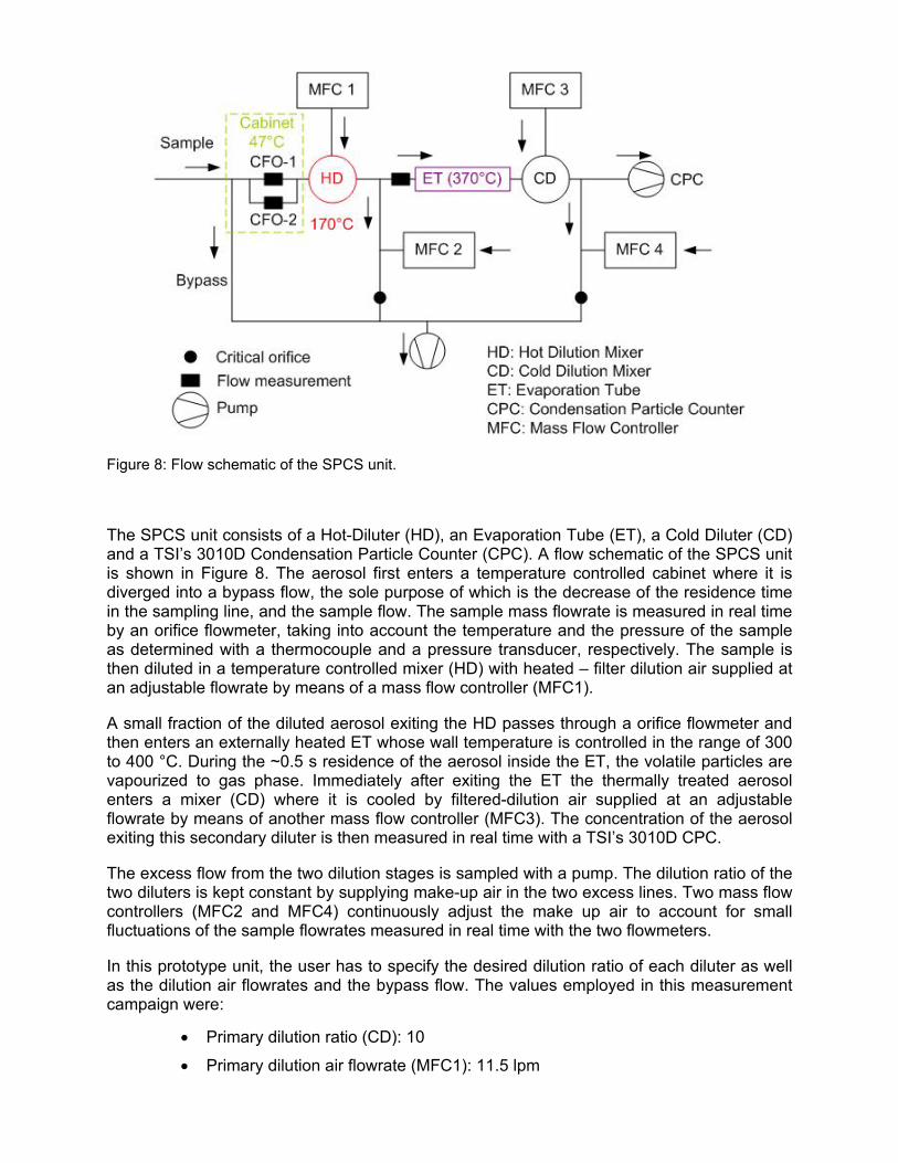
Figure 8: Flow schematic of the SPCS unit.

The SPCS unit consists of a Hot-Diluter (HD), an Evaporation Tube (ET), a Cold Diluter (CD) and a TSI’s 3010D Condensation Particle Counter (CPC). A flow schematic of the SPCS unit is shown in Figure 8. The aerosol first enters a temperature controlled cabinet where it is diverged into a bypass flow, the sole purpose of which is the decrease of the residence time in the sampling line, and the sample flow. The sample mass flowrate is measured in real time by an orifice flowmeter, taking into account the temperature and the pressure of the sample as determined with a thermocouple and a pressure transducer, respectively. The sample is then diluted in a temperature controlled mixer (HD) with heated – filter dilution air supplied at an adjustable flowrate by means of a mass flow controller (MFC1).

A small fraction of the diluted aerosol exiting the HD passes through a orifice flowmeter and then enters an externally heated ET whose wall temperature is controlled in the range of 300 to 400 °C. During the ~0.5 s residence of the aerosol inside the ET, the volatile particles are vapourized to gas phase. Immediately after exiting the ET the thermally treated aerosol enters a mixer (CD) where it is cooled by filtered-dilution air supplied at an adjustable flowrate by means of another mass flow controller (MFC3). The concentration of the aerosol exiting this secondary diluter is then measured in real time with a TSI’s 3010D CPC.

The excess flow from the two dilution stages is sampled with a pump. The dilution ratio of the two diluters is kept constant by supplying make-up air in the two excess lines. Two mass flow controllers (MFC2 and MFC4) continuously adjust the make up air to account for small fluctuations of the sample flowrates measured in real time with the two flowmeters.

In this prototype unit, the user has to specify the desired dilution ratio of each diluter as well as the dilution air flowrates and the bypass flow. The values employed in this measurement campaign were:

• Primary dilution ratio (CD): 10

• Primary dilution air flowrate (MFC1): 11.5 lpm

• Secondary dilution ratio (HD): 15

• Secondary dilution air flowrate (MFC3): 10.5 lpm

• Bypass flowrate: 2 lpm

The results obtained with the two instruments were corrected for the CPC slopes and the average Particle Concentration Reduction Factors (PCRF) at 30, 50 and 100 nm (in accordance to the legislation) that were determined after the measurement campaign in the framework of the PMP VPR calibration exercise. The measured PCRF values were 218 (±5), 209 (±2) and 205 (±2) at 30 nm, 50 nm and 100 nm, respectively. These figures are consistently higher from those measured 2 year ago (Giechaskiel et al. 2009b), siuggesting a drift of the average PCRF by 13%. This shift was also verified by gas measurements of the dilution factor and is most probably associated with fouling of the critical orifices. The results of these investigations will be presented in a separate report.

2.2.4.2 TSI’s 3936L10 Scanning Mobility Particle Sizer

A TSI’s 3936L10 Scanning Mobility Particle Sizer (SMPS) was employed in a limited number of tests for the measurement of the number weighted mobility size distributions. The core of the SMPS unit is a TSI’s 3081 cylindrical Differential Mobility Analyzer (DMA) for size classification that is followed by a TSI’s 3010 CPC for particle detection. The sampled aerosol was charged in a 10 mCi neutralizer manufactured by Eckert and Ziegler GmbH. An impactor having a cut-off size above 1 μm (0.071 cm nozzle – TSI part number 1508111) was employed at the inlet of instrument to remove very large particles but also to monitor the sample flowrate through the measurement of the induced pressure drop. The operating flowrates were regularly checked during the measurement campaign with a bubble flowmeter (Gillian Gillibrator – 2). The measured sample flow rate (which was consistently measured to be 0.96 lpm), was employed for the data inversion.

The SMPS operated on a sheath over sample flow rate setting of 10 lpm over 1 lpm and a scan time of 90 s in all engine tests. These settings allows for the determination of the size distribution in the size range of 7.5 nm to 294.3 nm. The size distributions were acquired using TSI’s software (AIM 8.1.0.0), which takes into account particle losses inside the instrument. The performance of the SMPS unit was checked during the second phase of the PEMS-PM programme (Mamakos et al. 2011), where it was found to classify particle sizes with an accuracy of better than 1%. The CPC indications were accordingly corrected for the 15% slope determined in these experiments.

2.2.4.3 Sunset Laboratory OC-EC Aerosol Analyzer

The Laboratory OC-EC Aerosol Analyzer by Sunset Laboratory was used to analyze aerosol particles collected on quartz-fiber filters for the quantification of the organic and elemental carbon content of PM (Birch et al. 1996). This instrument uses a thermal-optical method to analyze the EC and OC collected on quartz filters. Samples are thermally desorbed from the filter medium under an inert helium atmosphere followed by an oxidizing atmosphere using carefully controlled heating ramps. By careful system control and continuous monitoring of the optical absorbance of the sample during analysis, this method is able to both prevent any undesired oxidation of original elemental carbon and make corrections for the inevitable

generation of carbon char produced by the pyrolitic conversion of organics into elemental carbon.

47 mm Quartz-fiber filters were employed. The punch used for the analysis was 1.0 by 1.5 cm in size. The stain area, required for the deduction of PM emissions, was measured to be 11.34 cm2 for the filter holder employed. The detection limit of the method is 0.2 μg/cm2 which corresponds to a PM level of ~0.5 mg/kWh. Due to the very small background level of the filters employed (2500QAO-UP – Pall Corp.), it was not necessary to pre-bake the filters. The background levels, measured by analyzing a blank filter coming from the same batch, were determined to be 0.43 μg/cm2 OC and 0.00 μg/cm2. Results presented in this report have been corrected for this background.

2.2.5 Aerosol Generators

2.2.5.1 PALAS DNP 3000 spark generator

The PALAS DNP 3000 generator (Figure 9) operates on the principle of electrical discharge (Schwyn et al. 1988). A high voltage is applied between two graphite electrodes producing a spark that results in evaporation of small quantities of graphite. To avoid oxidation of the graphite, a nitrogen stream is focused through a narrow slit into the space between the two electrodes. The graphite evaporating in these sparks is transported by the nitrogen flow and condenses to fine primary particles as the temperature drops down. These particles subsequently coagulate forming complex aggregates. The rate of coagulation, and correspondingly the size of the aggregates, depends on the concentration of the primary particles which can be adjusted by means of controlling the spark frequency. The concentration of the aggregates can be controlled by means of adding some dilution air. The electrode consumption is compensated by an automatic adjustment of the electrodes. The settings employed in these experiments were 3 lpm N2 flow, 3 lpm dilution air flow and 2 mA current (output current of the high voltage supply unit).

Figure 9: PALAS DNP3000 spark generator

2.2.5.2 Oil Particle Generator

A JRC prototype oil particle generator (Figure 10) was employed for the production of Poly-Alpha-Olephin (PAO) particles. The operation principle is based on the evaporation condensation technique. The PAO oil is placed in a metal crucible in which is heated through an electric Bunsen near its boiling point. A small flow of nitrogen is introduced into the crucible to displace vapor from the surface of the bulk material to a cooler region of the generator where it mixes with carrier gas flow and condenses. The size and concentration of

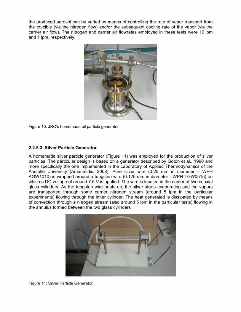
the produced aerosol can be varied by means of controlling the rate of vapor transport from the crucible (via the nitrogen flow) and/or the subsequent cooling rate of the vapor (via the carrier air flow). The nitrogen and carrier air flowrates employed in these tests were 10 lpm and 1 lpm, respectively.

Figure 10: JRC’s homemade oil particle generator

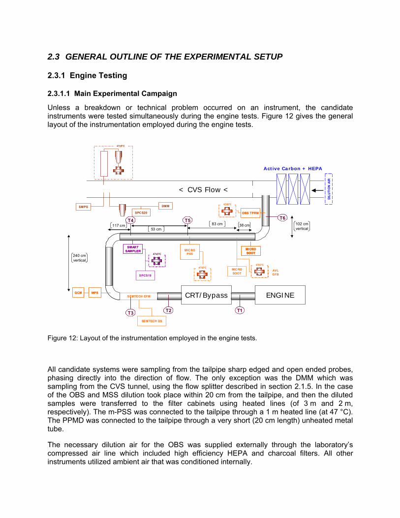
2.2.5.3 Silver Particle Generator

A homemade silver particle generator (Figure 11) was employed for the production of silver particles. The particular design is based on a generator described by Gotoh et al., 1990 and more specifically the one implemented in the Laboratory of Applied Thermodynamics of the Aristotle University (Amanatidis, 2008). Pure silver wire (0.25 mm in diameter – WPH AGW1010) is wrapped around a tungsten wire (0.125 mm in diameter - WPH TGW0515) on which a DC voltage of around 7.5 V is applied. The wire is located in the center of two coaxial glass cylinders. As the tungsten wire heats up, the silver starts evaporating and the vapors are transported through some carrier nitrogen stream (around 5 lpm in the particular experiments) flowing through the inner cylinder. The heat generated is dissipated by means of convection through a nitrogen stream (also around 5 lpm in the particular tests) flowing in the annulus formed between the two glass cylinders

Figure 11: Silver Particle Generator

2.3 GENERAL OUTLINE OF THE EXPERIMENTAL SETUP

2.3.1 Engine Testing

2.3.1.1 Main Experimental Campaign

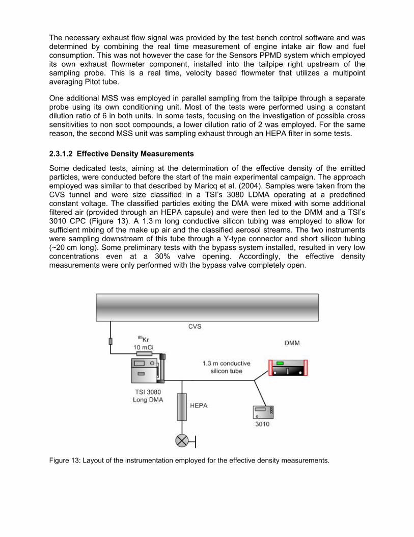
Unless a breakdown or technical problem occurred on an instrument, the candidate instruments were tested simultaneously during the engine tests. Figure 12 gives the general layout of the instrumentation employed during the engine tests.

ENGINECRT/BypassSEMTECH EFMMPSQCM MPSQCM

SMARTSAMPLER

SMARTSAMPLER

< CVS Flow <

Active Carbon + HEPA

SEMTECH DS

OBS TPRMOBS TPRM

MICROPSS

MICROPSS

T1T1T2T2T3T3

T4T4 T5T5 T6T6

47±5°C47±5°C

47±5°C47±5°C

47±5°C47±5°C

47±5°C

SMPS

DIL

UTI

ON

AIR

MICROSOOTMICROSOOTMICROSOOT

117 cm53 cm

83 cm 38 cm 102 cmvertical

240 cmvertical

SPCS19

47±5°C47±5°C

MICROSOOT

SPCS20

DMM

AVL GFB

Figure 12: Layout of the instrumentation employed in the engine tests.

All candidate systems were sampling from the tailpipe sharp edged and open ended probes, phasing directly into the direction of flow. The only exception was the DMM which was sampling from the CVS tunnel, using the flow splitter described in section 2.1.5. In the case of the OBS and MSS dilution took place within 20 cm from the tailpipe, and then the diluted samples were transferred to the filter cabinets using heated lines (of 3 m and 2 m, respectively). The m-PSS was connected to the tailpipe through a 1 m heated line (at 47 °C). The PPMD was connected to the tailpipe through a very short (20 cm length) unheated metal tube.

The necessary dilution air for the OBS was supplied externally through the laboratory’s compressed air line which included high efficiency HEPA and charcoal filters. All other instruments utilized ambient air that was conditioned internally.

The necessary exhaust flow signal was provided by the test bench control software and was determined by combining the real time measurement of engine intake air flow and fuel consumption. This was not however the case for the Sensors PPMD system which employed its own exhaust flowmeter component, installed into the tailpipe right upstream of the sampling probe. This is a real time, velocity based flowmeter that utilizes a multipoint averaging Pitot tube.

One additional MSS was employed in parallel sampling from the tailpipe through a separate probe using its own conditioning unit. Most of the tests were performed using a constant dilution ratio of 6 in both units. In some tests, focusing on the investigation of possible cross sensitivities to non soot compounds, a lower dilution ratio of 2 was employed. For the same reason, the second MSS unit was sampling exhaust through an HEPA filter in some tests.

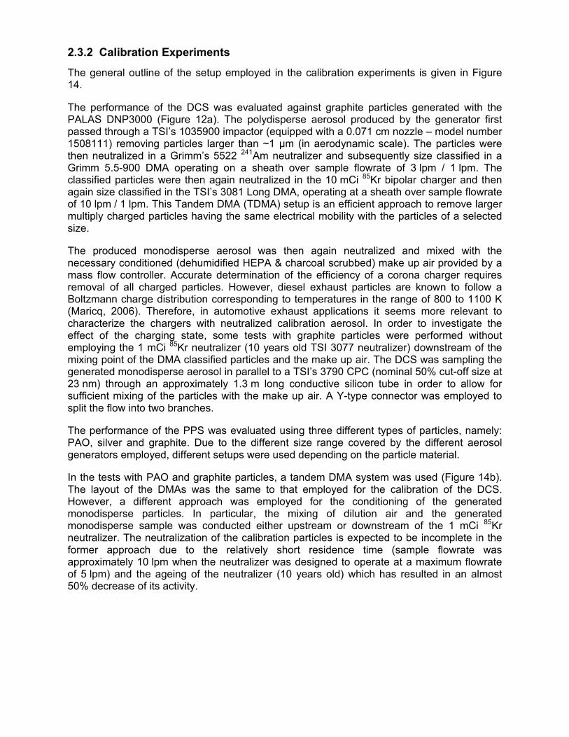
2.3.1.2 Effective Density Measurements

Some dedicated tests, aiming at the determination of the effective density of the emitted particles, were conducted before the start of the main experimental campaign. The approach employed was similar to that described by Maricq et al. (2004). Samples were taken from the CVS tunnel and were size classified in a TSI’s 3080 LDMA operating at a predefined constant voltage. The classified particles exiting the DMA were mixed with some additional filtered air (provided through an HEPA capsule) and were then led to the DMM and a TSI’s 3010 CPC (Figure 13). A 1.3 m long conductive silicon tubing was employed to allow for sufficient mixing of the make up air and the classified aerosol streams. The two instruments were sampling downstream of this tube through a Y-type connector and short silicon tubing (~20 cm long). Some preliminary tests with the bypass system installed, resulted in very low concentrations even at a 30% valve opening. Accordingly, the effective density measurements were only performed with the bypass valve completely open.

Figure 13: Layout of the instrumentation employed for the effective density measurements.

2.3.2 Calibration Experiments

The general outline of the setup employed in the calibration experiments is given in Figure 14.

The performance of the DCS was evaluated against graphite particles generated with the PALAS DNP3000 (Figure 12a). The polydisperse aerosol produced by the generator first passed through a TSI’s 1035900 impactor (equipped with a 0.071 cm nozzle – model number 1508111) removing particles larger than ~1 μm (in aerodynamic scale). The particles were then neutralized in a Grimm’s 5522 241Am neutralizer and subsequently size classified in a Grimm 5.5-900 DMA operating on a sheath over sample flowrate of 3 lpm / 1 lpm. The classified particles were then again neutralized in the 10 mCi 85Kr bipolar charger and then again size classified in the TSI’s 3081 Long DMA, operating at a sheath over sample flowrate of 10 lpm / 1 lpm. This Tandem DMA (TDMA) setup is an efficient approach to remove larger multiply charged particles having the same electrical mobility with the particles of a selected size.

The produced monodisperse aerosol was then again neutralized and mixed with the necessary conditioned (dehumidified HEPA & charcoal scrubbed) make up air provided by a mass flow controller. Accurate determination of the efficiency of a corona charger requires removal of all charged particles. However, diesel exhaust particles are known to follow a Boltzmann charge distribution corresponding to temperatures in the range of 800 to 1100 K (Maricq, 2006). Therefore, in automotive exhaust applications it seems more relevant to characterize the chargers with neutralized calibration aerosol. In order to investigate the effect of the charging state, some tests with graphite particles were performed without employing the 1 mCi 85Kr neutralizer (10 years old TSI 3077 neutralizer) downstream of the mixing point of the DMA classified particles and the make up air. The DCS was sampling the generated monodisperse aerosol in parallel to a TSI’s 3790 CPC (nominal 50% cut-off size at 23 nm) through an approximately 1.3 m long conductive silicon tube in order to allow for sufficient mixing of the particles with the make up air. A Y-type connector was employed to split the flow into two branches.

The performance of the PPS was evaluated using three different types of particles, namely: PAO, silver and graphite. Due to the different size range covered by the different aerosol generators employed, different setups were used depending on the particle material.

In the tests with PAO and graphite particles, a tandem DMA system was used (Figure 14b). The layout of the DMAs was the same to that employed for the calibration of the DCS. However, a different approach was employed for the conditioning of the generated monodisperse particles. In particular, the mixing of dilution air and the generated monodisperse sample was conducted either upstream or downstream of the 1 mCi 85Kr neutralizer. The neutralization of the calibration particles is expected to be incomplete in the former approach due to the relatively short residence time (sample flowrate was approximately 10 lpm when the neutralizer was designed to operate at a maximum flowrate of 5 lpm) and the ageing of the neutralizer (10 years old) which has resulted in an almost 50% decrease of its activity.

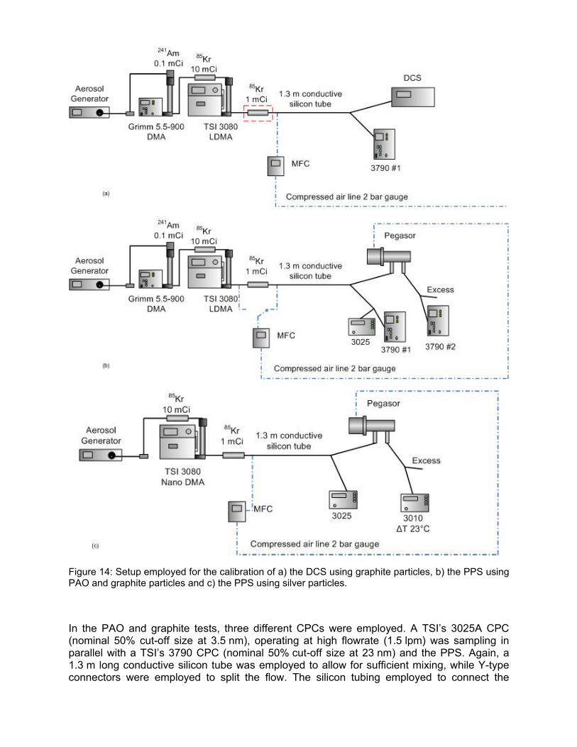
Figure 14: Setup employed for the calibration of a) the DCS using graphite particles, b) the PPS using PAO and graphite particles and c) the PPS using silver particles.

In the PAO and graphite tests, three different CPCs were employed. A TSI’s 3025A CPC (nominal 50% cut-off size at 3.5 nm), operating at high flowrate (1.5 lpm) was sampling in parallel with a TSI’s 3790 CPC (nominal 50% cut-off size at 23 nm) and the PPS. Again, a 1.3 m long conductive silicon tube was employed to allow for sufficient mixing, while Y-type connectors were employed to split the flow. The silicon tubing employed to connect the

instruments to the Y-type connectors was kept as low as possible (maximum ~25 cm), given the space limitations. A second 3790 CPC was also connected to the outlet of the PPS. A comparison of the responses of the two 3790 CPCs allowed for the quantification of particle penetration through the PPS as a function of size and trap voltage applied.

The setup employed for the calibration of the PPS against silver particles is shown in Figure 14c. The silver particle generator produces very small particles (smaller than 30 nm) which practically do not carry more than 1 elemental charge. Therefore it was not necessary to employ a Tandem DMA setup. For these particular measurements, what is of importance is to minimize diffusion losses. To this end, a TSI’s 3085 Nano DMA was employed to size classify the calibration aerosol. Additionally, the 3790 CPCs are not suited for this type of measurements as they have a relatively large cut-off size (~23 nm). The TSI’s 3010 CPC, operating at an elevated saturator-condenser temperature difference of 23°C, was employed instead in order to monitor the concentration of particles exiting the PPS. The responses of the 3010 and 3025A CPCs were cross-compared in separate tests with silver particles at the three different sizes investigated (10, 15 and 20 nm) and the relative differences were accounted for in the evaluation of the data.

The necessary dilution air for the PPS was supplied externally through the laboratory’s compressed air line, at a gauge pressure of 2 bar, following the manufacturer’s specifications. The dilution air was filtered (through an HEPA capsule), charcoal scrubbed and dehumidified. Preliminary checks at the end of main experimental phase suggested that the corona wire was corroded, as evident from a very low corona current. Following manufacturer’s recommendation, the corona wire of the PPS was replaced before the calibration experiments. The flows of the DMAs and the instrumentation were measured before and after the tests with a bubble flowmeter (Gillian Gilibrator-2). The CPCs employed were calibrated in the framework of the PMP VPR calibration activity. The results obtained were corrected for the differences in the detection efficiency curves and the slopes if the CPCs. The results of these calibrations will be reported elsewhere.

2.4 TEST PROCEDURES The daily engine measurement protocol included four repetitions of the World Harmonized Transient Cycle (WHTC) test cycle all performed with the engine hot. The engine was warmed up before the first test to increase the oil temperature above 65°C, by means of running the engine over ESC mode 7. The subsequent two WHTC were performed immediately after the completion of the first WHTC cycle. During these three tests repetitions, a single PM filter was employed in the CVS tunnel, the laboratory PFDS and the different PEMS-PM candidate systems (m-PSS, AVL GFB and OBS). A fourth WHTC test cycle was performed in the afternoon, following the same engine warm-up procedure. A different PM filter was employed over the particular test.

Measurements have been conducted at five different particulate emission levels corresponding to DPF out (no bypass), and four different bypass valve positions resulting in PM emission levels at a Euro V level (30% valve opening), a Euro VI level (5% valve opening) and two intermediate levels (10% and 2% valve opening). The daily test procedure was repeated 4 times at each configuration (with the exception of the 10% valve opening for which only two repetitions were performed) in order to establish the repeatability of each candidate PEMS system results but also investigate the effect of filter media on PM. In particular, two repetitions were performed employing Teflon filters, one repetition using TX40 filters and a final one using Quartz filters in the CVS tunnel and TX40 filters in the SPC and

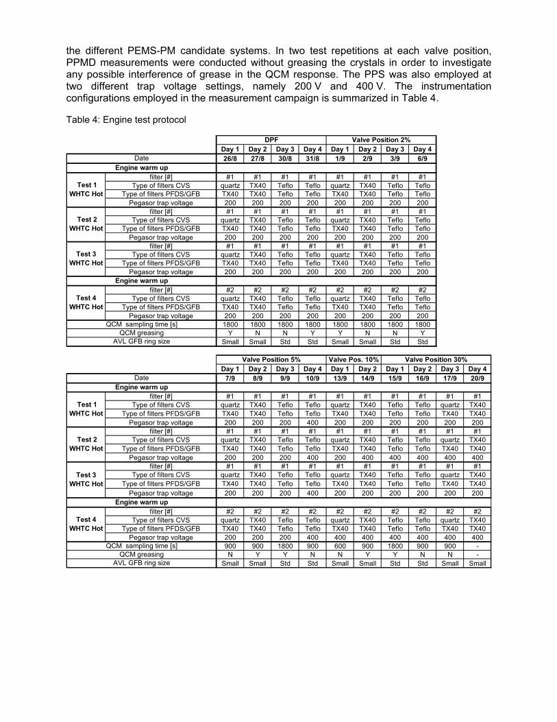
the different PEMS-PM candidate systems. In two test repetitions at each valve position, PPMD measurements were conducted without greasing the crystals in order to investigate any possible interference of grease in the QCM response. The PPS was also employed at two different trap voltage settings, namely 200 V and 400 V. The instrumentation configurations employed in the measurement campaign is summarized in Table 4.

Table 4: Engine test protocol

Day 1 Day 2 Day 3 Day 4 Day 1 Day 2 Day 3 Day 426/8 27/8 30/8 31/8 1/9 2/9 3/9 6/9

filter [#] #1 #1 #1 #1 #1 #1 #1 #1Type of filters CVS quartz TX40 Teflo Teflo quartz TX40 Teflo Teflo

Type of filters PFDS/GFB TX40 TX40 Teflo Teflo TX40 TX40 Teflo TefloPegasor trap voltage 200 200 200 200 200 200 200 200







1800 1800 1800 1800 1800 1800 1800 1800Y N N Y Y N N Y

Small Small Std Std Small Small Std Std

Day 1 Day 2 Day 3 Day 4 Day 1 Day 2 Day 1 Day 2 Day 3 Day 47/9 8/9 9/9 10/9 13/9 14/9 15/9 16/9 17/9 20/9

filter [#] #1 #1 #1 #1 #1 #1 #1 #1 #1 #1Type of filters CVS quartz TX40 Teflo Teflo quartz TX40 Teflo Teflo quartz TX40

Type of filters PFDS/GFB TX40 TX40 Teflo Teflo TX40 TX40 Teflo Teflo TX40 TX40Pegasor trap voltage 200 200 200 400 200 200 200 200 200 200







900 900 1800 900 600 900 1800 900 900 -N Y Y N N Y Y N N -

Small Small Std Std Small Small Std Std Small SmallAVL GFB ring size

Test 2 WHTC Hot

Test 3 WHTC Hot

Engine warm up

Test 4 WHTC Hot

QCM sampling time [s]QCM greasing

Valve Position 5% Valve Pos. 10% Valve Position 30%

Engine warm up

Test 1 WHTC Hot

Date

AVL GFB ring size

Engine warm up

QCM greasingQCM sampling time [s]

DPF Valve Position 2%

Engine warm upDate

Test 1 WHTC Hot

Test 2 WHTC Hot

Test 3 WHTC Hot

Test 4 WHTC Hot

3 EXPERIMENTAL RESULTS

3.1 REFERENCE LABORATORY INSTRUMENTATION This section describes in some detail the results obtained with the reference laboratory instrumentation, in order to get some insight on the emission levels and the nature of PM at the different aftertreatment configurations employed.

3.1.1 PM emissions

Figure 15 summarizes the PM emission results determined from the CVS (left-hand panels) and SPC (right hand panels). Each bar corresponds to the cycle-average emissions while the error bands correspond to ± one standard error (defined as the standard deviation divided by the square root of the number of test repetitions). The thermogravimetrically determined emissions from the quartz samples provided the means to also quantify the EC content of the emitted PM.

PM emissions spanned from a value close to the Euro V emission standard of 20 mg/kWh at 30% valve opening, to 1-6 mg/kWh at a DPF out level. The total carbon (TC) mass determined from the thermogravimetric analysis of quartz filters were found to be in very good agreement with the PM emissions determined from samples collected on TX40 filters, the individual differences being on average -1% (±29%). Teflon filters yielded systematically lower PM emissions, with the difference increasing with decreasing PM levels.

The individual differences of the PM emission levels determined with TX40 filters and the TC, from the PM results determined from Teflon filters are plotted in Figure 16. The difference increases nonlinearly with decreasing PM levels from 20%-60% at 30% valve opening (~20 mg/kWh) to as high as 300%-760% at DPF out levels. The differences were 60% (±19%) lower when a single filter was employed over three consecutive WHTC cycles, ranging from 17% to 26% at 30% valve opening to 150%-360% at DPF out levels. The trends were similar for both CVS and SPC samples.

The thermogravimetric analysis of the quartz samples suggested a gradually decreasing contribution of EC with decreasing PM levels. The EC content of the quartz samples over a single WHTC decreased from 52%, 37%, 11% at 30%, 10% and 2% bypass valve opening and practically 0% with the bypass completely closed. The use of a single Quartz filter over three consecutive WHTC tests increased the EC content which ranged from 70% at 30% bypass valve opening to 30% at 2% bypass valve opening, but it still remained practically zero at DPF out levels. The mass of this volatile PM emitted downstream of the DPF averaged at 0.9 (±0.7) mg/kWh when Teflon filters were employed and 4.6 (±1.5) mg/kWh when TX40 filters were used.

The observed discrepancies between Teflon and TX40, Quartz results is indicative of a gaseous adsorption artefact, which is known to be less pronounced when Teflon filters are employed (Chase et al. 2004).

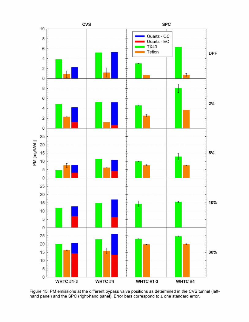
Figure 15: PM emissions at the different bypass valve positions as determined in the CVS tunnel (left-hand panel) and the SPC (right-hand panel). Error bars correspond to ± one standard error.

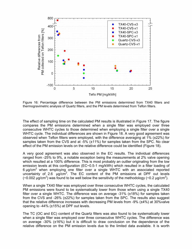
Figure 16: Percentage difference between the PM emissions determined from TX40 filters and thermogravimetric analysis of Quartz filters, and the PM levels determined from Teflon filters.

The effect of sampling time on the calculated PM results is illustrated in Figure 17. The figure compares the PM emissions determined when a single filter was employed over three consecutive WHTC cycles to those determined when employing a single filter over a single WHTC cycle. The individual differences are shown in Figure 18. A very good agreement was observed when Teflon filters were employed, with the difference averaging at 1% (±22%) for samples taken from the CVS and at -5% (±11%) for samples taken from the SPC. No clear effect of the PM emission levels on the relative difference could be identified (Figure 18).

A very good agreement was also observed in the EC results. The individual differences ranged from -25% to 9%, a notable exception being the measurements at 2% valve opening which resulted at a 100% difference. This is most probably an outlier originating from the low emission levels at this configuration (EC~0.5-1 mg/kWh) which resulted in a filter loading of 6 μg/cm2 when employing one filter over a single WHTC with an associated reported uncertainty of 2.6 μg/cm2. The EC content of the PM emissions at DPF out levels (~0.002 μg/cm2) was found to be well below the sensitivity of the methodology (~0.2 μg/cm2).

When a single TX40 filter was employed over three consecutive WHTC cycles, the calculated PM emissions were found to be systematically lower from those when using a single TX40 filter over a single WHTC. The difference was on average -31% (±18%) for samples taken from the CVS and -26% (±22%) for samples taken from the SPC. The results also suggest that the relative difference increases with decreasing PM levels from -9% (±4%) at 30%valve opening to -44% (±15%) at DPF out levels.

The TC (OC and EC) content of the Quartz filters was also found to be systematically lower when a single filter was employed over three consecutive WHTC cycles. The difference was on average -30% (±16%) but it is difficult to draw conclusion on the dependence of the relative difference on the PM emission levels due to the limited data available. It is worth

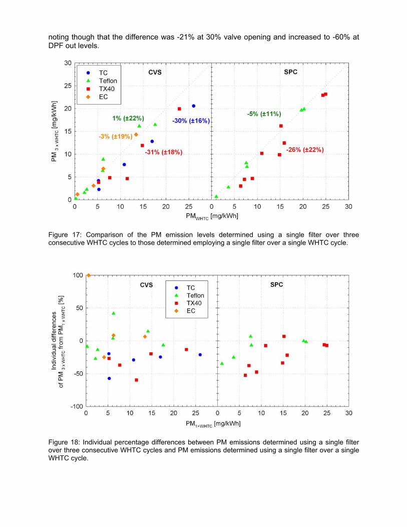
noting though that the difference was -21% at 30% valve opening and increased to -60% at DPF out levels.

Figure 17: Comparison of the PM emission levels determined using a single filter over three consecutive WHTC cycles to those determined employing a single filter over a single WHTC cycle.

Figure 18: Individual percentage differences between PM emissions determined using a single filter over three consecutive WHTC cycles and PM emissions determined using a single filter over a single WHTC cycle.

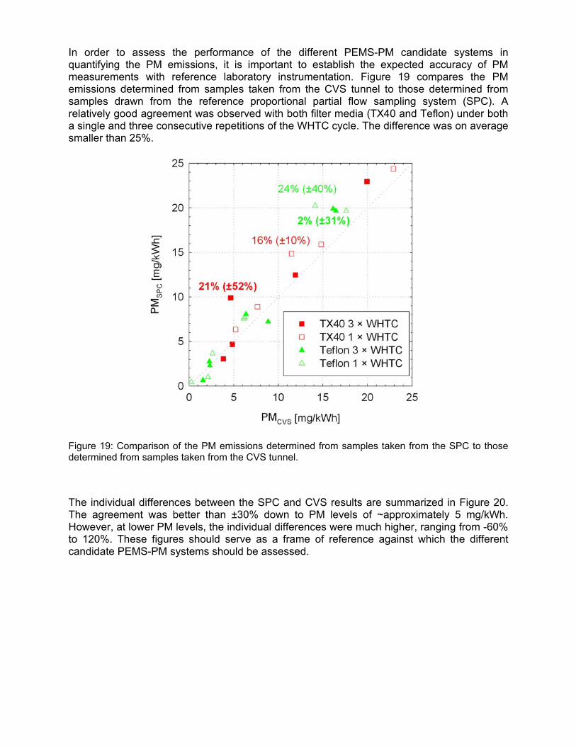
In order to assess the performance of the different PEMS-PM candidate systems in quantifying the PM emissions, it is important to establish the expected accuracy of PM measurements with reference laboratory instrumentation. Figure 19 compares the PM emissions determined from samples taken from the CVS tunnel to those determined from samples drawn from the reference proportional partial flow sampling system (SPC). A relatively good agreement was observed with both filter media (TX40 and Teflon) under both a single and three consecutive repetitions of the WHTC cycle. The difference was on average smaller than 25%.

Figure 19: Comparison of the PM emissions determined from samples taken from the SPC to those determined from samples taken from the CVS tunnel.

The individual differences between the SPC and CVS results are summarized in Figure 20. The agreement was better than ±30% down to PM levels of ~approximately 5 mg/kWh. However, at lower PM levels, the individual differences were much higher, ranging from -60% to 120%. These figures should serve as a frame of reference against which the different candidate PEMS-PM systems should be assessed.

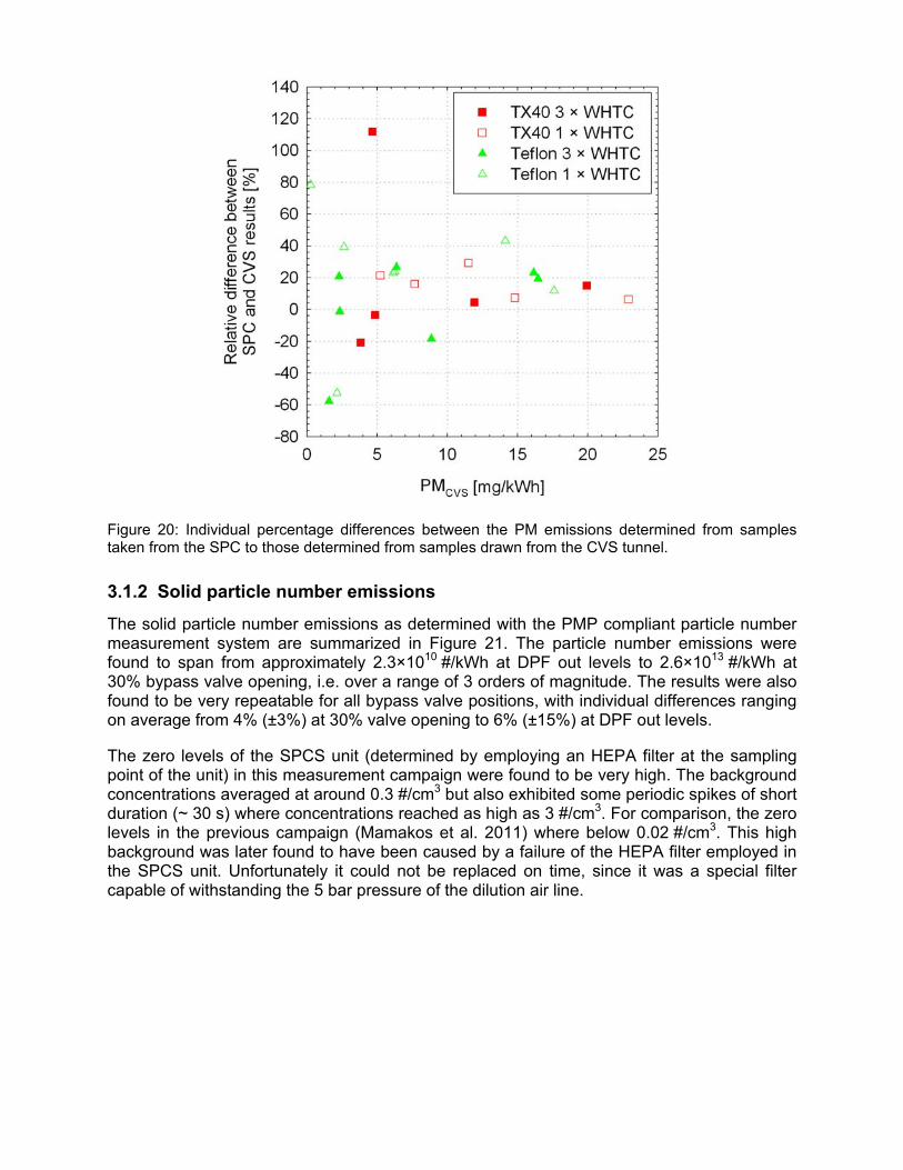
Figure 20: Individual percentage differences between the PM emissions determined from samples taken from the SPC to those determined from samples drawn from the CVS tunnel.

3.1.2 Solid particle number emissions

The solid particle number emissions as determined with the PMP compliant particle number measurement system are summarized in Figure 21. The particle number emissions were found to span from approximately 2.3×1010 #/kWh at DPF out levels to 2.6×1013 #/kWh at 30% bypass valve opening, i.e. over a range of 3 orders of magnitude. The results were also found to be very repeatable for all bypass valve positions, with individual differences ranging on average from 4% (±3%) at 30% valve opening to 6% (±15%) at DPF out levels.

The zero levels of the SPCS unit (determined by employing an HEPA filter at the sampling point of the unit) in this measurement campaign were found to be very high. The background concentrations averaged at around 0.3 #/cm3 but also exhibited some periodic spikes of short duration (~ 30 s) where concentrations reached as high as 3 #/cm3. For comparison, the zero levels in the previous campaign (Mamakos et al. 2011) where below 0.02 #/cm3. This high background was later found to have been caused by a failure of the HEPA filter employed in the SPCS unit. Unfortunately it could not be replaced on time, since it was a special filter capable of withstanding the 5 bar pressure of the dilution air line.

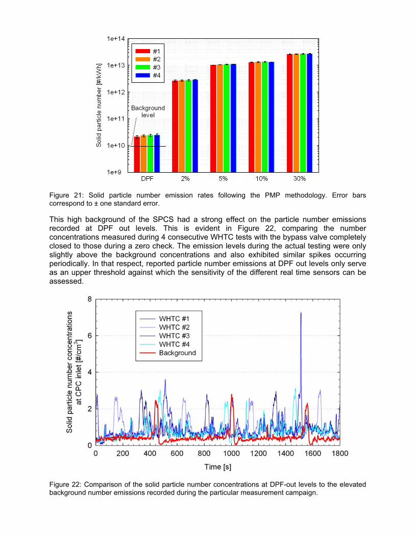
Figure 21: Solid particle number emission rates following the PMP methodology. Error bars correspond to ± one standard error.

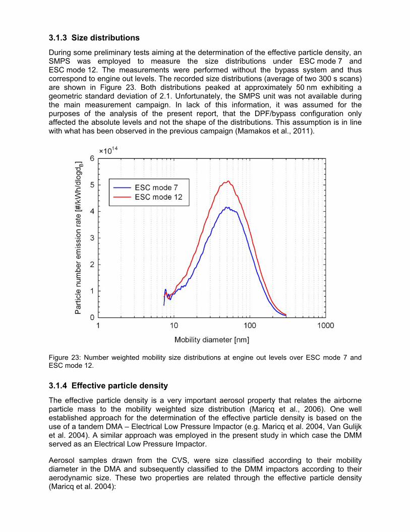
This high background of the SPCS had a strong effect on the particle number emissions recorded at DPF out levels. This is evident in Figure 22, comparing the number concentrations measured during 4 consecutive WHTC tests with the bypass valve completely closed to those during a zero check. The emission levels during the actual testing were only slightly above the background concentrations and also exhibited similar spikes occurring periodically. In that respect, reported particle number emissions at DPF out levels only serve as an upper threshold against which the sensitivity of the different real time sensors can be assessed.

Figure 22: Comparison of the solid particle number concentrations at DPF-out levels to the elevated background number emissions recorded during the particular measurement campaign.

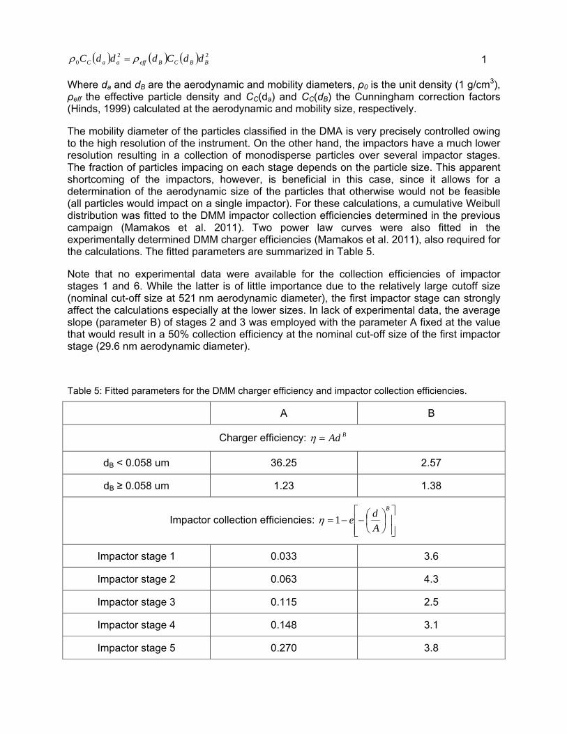
3.1.3 Size distributions

During some preliminary tests aiming at the determination of the effective particle density, an SMPS was employed to measure the size distributions under ESC mode 7 and ESC mode 12. The measurements were performed without the bypass system and thus correspond to engine out levels. The recorded size distributions (average of two 300 s scans) are shown in Figure 23. Both distributions peaked at approximately 50 nm exhibiting a geometric standard deviation of 2.1. Unfortunately, the SMPS unit was not available during the main measurement campaign. In lack of this information, it was assumed for the purposes of the analysis of the present report, that the DPF/bypass configuration only affected the absolute levels and not the shape of the distributions. This assumption is in line with what has been observed in the previous campaign (Mamakos et al., 2011).

Figure 23: Number weighted mobility size distributions at engine out levels over ESC mode 7 and ESC mode 12.

3.1.4 Effective particle density

The effective particle density is a very important aerosol property that relates the airborne particle mass to the mobility weighted size distribution (Maricq et al., 2006). One well established approach for the determination of the effective particle density is based on the use of a tandem DMA – Electrical Low Pressure Impactor (e.g. Maricq et al. 2004, Van Gulijk et al. 2004). A similar approach was employed in the present study in which case the DMM served as an Electrical Low Pressure Impactor.

Aerosol samples drawn from the CVS, were size classified according to their mobility diameter in the DMA and subsequently classified to the DMM impactors according to their aerodynamic size. These two properties are related through the effective particle density (Maricq et al. 2004):

( ) ( ) ( ) 220 BBCBeffaaC ddCdddC ρρ = 1

Where da and dB are the aerodynamic and mobility diameters, ρ0 is the unit density (1 g/cm3), ρeff the effective particle density and CC(da) and CC(dB) the Cunningham correction factors (Hinds, 1999) calculated at the aerodynamic and mobility size, respectively.

The mobility diameter of the particles classified in the DMA is very precisely controlled owing to the high resolution of the instrument. On the other hand, the impactors have a much lower resolution resulting in a collection of monodisperse particles over several impactor stages. The fraction of particles impacing on each stage depends on the particle size. This apparent shortcoming of the impactors, however, is beneficial in this case, since it allows for a determination of the aerodynamic size of the particles that otherwise would not be feasible (all particles would impact on a single impactor). For these calculations, a cumulative Weibull distribution was fitted to the DMM impactor collection efficiencies determined in the previous campaign (Mamakos et al. 2011). Two power law curves were also fitted in the experimentally determined DMM charger efficiencies (Mamakos et al. 2011), also required for the calculations. The fitted parameters are summarized in Table 5.

Note that no experimental data were available for the collection efficiencies of impactor stages 1 and 6. While the latter is of little importance due to the relatively large cutoff size (nominal cut-off size at 521 nm aerodynamic diameter), the first impactor stage can strongly affect the calculations especially at the lower sizes. In lack of experimental data, the average slope (parameter B) of stages 2 and 3 was employed with the parameter A fixed at the value that would result in a 50% collection efficiency at the nominal cut-off size of the first impactor stage (29.6 nm aerodynamic diameter).

Table 5: Fitted parameters for the DMM charger efficiency and impactor collection efficiencies.

A B

Charger efficiency: BAd=η

dB < 0.058 um 36.25 2.57

dB ≥ 0.058 um 1.23 1.38

Impactor collection efficiencies: ⎥⎥⎦

⎤

⎢⎢⎣

⎡⎟⎠⎞

⎜⎝⎛−−=

B

Ade1η

Impactor stage 1 0.033 3.6





The calculation procedure has as follows. At a first stage, the CPC and DMM signals were corrected for the presence of doubly charged particles as described in Maricq et al. (2004). This correction requires appropriate selection of the DMA classified sizes. The number concentration measured with the CPC was then translated to a current flux through the DMM charger efficiency calculated at the classified mobility diameter. Starting from an arbitrarily selected effective density value, the mobility diameter is translated to aerodynamic diameter through equation 1. The current flux was subsequently convoluted with the impactor collection efficiencies to simulate the DMM response at the given aerodynamic size. The procedure was then repeated for different values of effective density until the best much was obtained between the simulated and the measured DMM responses. The objective function employed in this optimization problem was:

( )∑=

−=6

1

2,,

iisimimeas IIOF 2

Where Imeas,i the measured current in impactor stage i, and Isim,i the simulated current in impactor stage i.

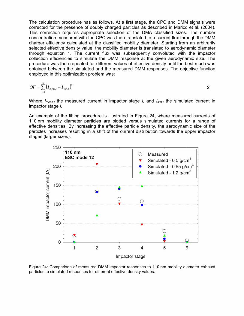
An example of the fitting procedure is illustrated in Figure 24, where measured currents of 110 nm mobility diameter particles are plotted versus simulated currents for a range of effective densities. By increasing the effective particle density, the aerodynamic size of the particles increases resulting in a shift of the current distribution towards the upper impactor stages (larger sizes).

Figure 24: Comparison of measured DMM impactor responses to 110 nm mobility diameter exhaust particles to simulated responses for different effective density values.

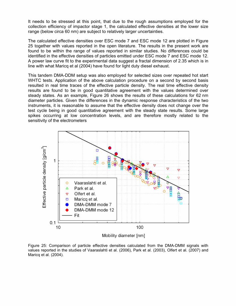
It needs to be stressed at this point, that due to the rough assumptions employed for the collection efficiency of impactor stage 1, the calculated effective densities at the lower size range (below circa 60 nm) are subject to relatively larger uncertainties.

The calculated effective densities over ESC mode 7 and ESC mode 12 are plotted in Figure 25 together with values reported in the open literature. The results in the present work are found to be within the range of values reported in similar studies. No differences could be identified in the effective densities of particles emitted under ESC mode 7 and ESC mode 12. A power law curve fit to the experimental data suggest a fractal dimension of 2.35 which is in line with what Maricq et al (2004) have found for light duty diesel exhaust.

This tandem DMA-DDM setup was also employed for selected sizes over repeated hot start WHTC tests. Application of the above calculation procedure on a second by second basis resulted in real time traces of the effective particle density. The real time effective density results are found to be in good quantitative agreement with the values determined over steady states. As an example, Figure 26 shows the results of these calculations for 62 nm diameter particles. Given the differences in the dynamic response characteristics of the two instruments, it is reasonable to assume that the effective density does not change over the test cycle being in good quantitative agreement with the steady state results. Some large spikes occurring at low concentration levels, and are therefore mostly related to the sensitivity of the electrometers

Figure 25: Comparison of particle effective densities calculated from the DMA-DMM signals with values reported in the studies of Vaaraslahti et al. (2006), Park et al. (2003), Olfert et al. (2007) and Maricq et al. (2004).

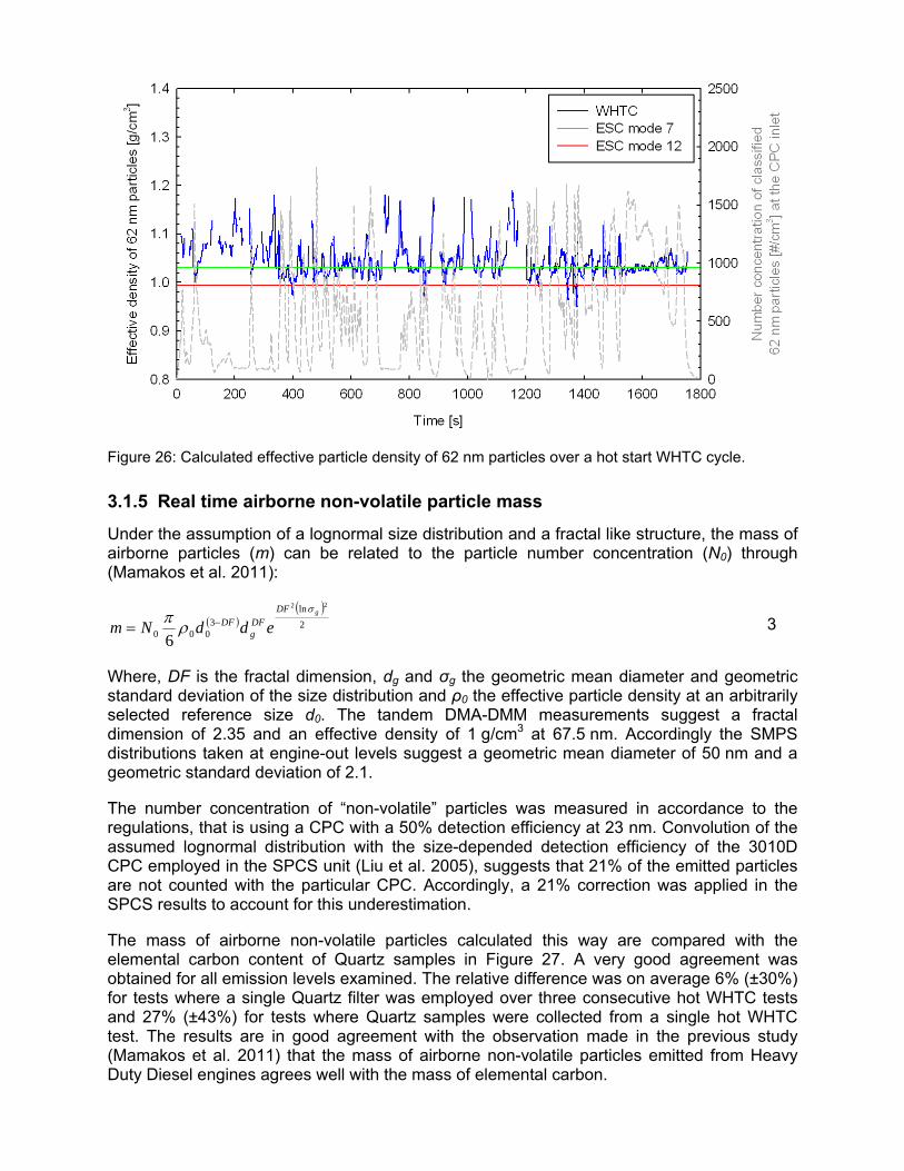
Figure 26: Calculated effective particle density of 62 nm particles over a hot start WHTC cycle.

3.1.5 Real time airborne non-volatile particle mass

Under the assumption of a lognormal size distribution and a fractal like structure, the mass of airborne particles (m) can be related to the particle number concentration (N0) through (Mamakos et al. 2011):

( )( )2ln

3000

22

6

gDFDFg

DF eddNmσ

ρπ −= 3

Where, DF is the fractal dimension, dg and σg the geometric mean diameter and geometric standard deviation of the size distribution and ρ0 the effective particle density at an arbitrarily selected reference size d0. The tandem DMA-DMM measurements suggest a fractal dimension of 2.35 and an effective density of 1 g/cm3 at 67.5 nm. Accordingly the SMPS distributions taken at engine-out levels suggest a geometric mean diameter of 50 nm and a geometric standard deviation of 2.1.

The number concentration of “non-volatile” particles was measured in accordance to the regulations, that is using a CPC with a 50% detection efficiency at 23 nm. Convolution of the assumed lognormal distribution with the size-depended detection efficiency of the 3010D CPC employed in the SPCS unit (Liu et al. 2005), suggests that 21% of the emitted particles are not counted with the particular CPC. Accordingly, a 21% correction was applied in the SPCS results to account for this underestimation.

The mass of airborne non-volatile particles calculated this way are compared with the elemental carbon content of Quartz samples in Figure 27. A very good agreement was obtained for all emission levels examined. The relative difference was on average 6% (±30%) for tests where a single Quartz filter was employed over three consecutive hot WHTC tests and 27% (±43%) for tests where Quartz samples were collected from a single hot WHTC test. The results are in good agreement with the observation made in the previous study (Mamakos et al. 2011) that the mass of airborne non-volatile particles emitted from Heavy Duty Diesel engines agrees well with the mass of elemental carbon.

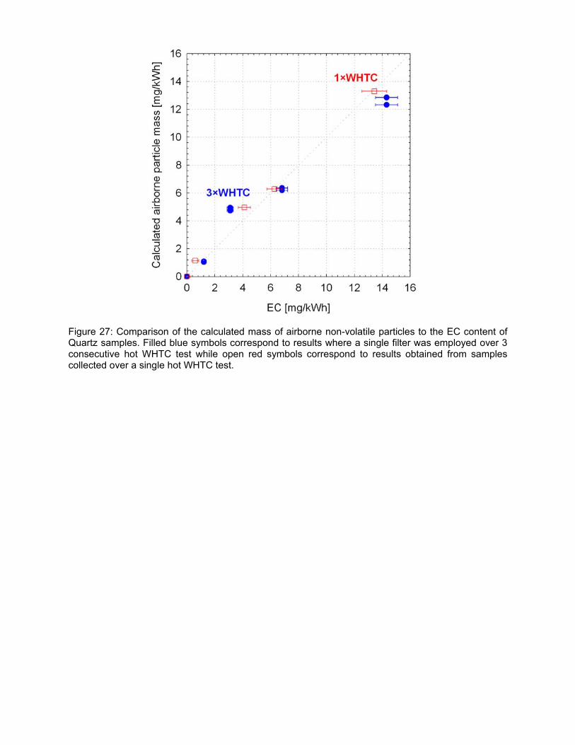
Figure 27: Comparison of the calculated mass of airborne non-volatile particles to the EC content of Quartz samples. Filled blue symbols correspond to results where a single filter was employed over 3 consecutive hot WHTC test while open red symbols correspond to results obtained from samples collected over a single hot WHTC test.

3.2 PPMD

3.2.1 Modifications

In the present study, the CQCM crystals were replaced by new ones provided by Sensors. Furthermore, longer sampling times were employed for each crystal of the CQCM, that ranged from 600 s at high PM levels to 1800 s at DPF out levels. Care was taken to randomize the sequence of crystal sampling at the different test repetitions.

The calculation of the CQCM was performed externally. Following a removal of spikes, regularly observed in the crystal responses, the real time traces were corrected for drifts caused by pressure, temperature and humidity fluctuations in the conditioning air, using the signal of a non-sampling crystal as a reference. The same reference crystal (crystal number 7) was employed as a reference in all tests. The mass collected during each sampling period was determined as the difference between the mass after and before sampling. As in the previous campaign (Mamakos et al. 2011), the calculations were performed employing all possible averaging and delay periods between 30-230 s and >10 s, respectively, using the average value as representative of the mass build up. No correction for thermophoretic or diffusion losses was employed.

3.2.2 Correlation of CQCM mass to PM and total carbon

Figure 28 compares the cycle average mass emission rates measured with the CQCM to the PM and TC emissions determined from CVS and SPC filter samples. The CQCM yielded on average higher mass emission rates from PM mass collected on Teflon filters. The difference was on average 59% (±126%) for CVS samples and 20% (±61%) for SPC samples. In contrast, the PM mass collected on TX40 filters and the TC content of Quartz filters was systematically higher from the CQCM mass. The difference was on average -13% (±82%) for CVS TX40 samples and -33% (±44%) for SPC TX40 samples. Thermogravimetric analysis of Quartz filters yielded a TC mass that was on average 20% lower the CQCM mass.

However, the individual differences, plotted in Figure 29, hardly show any trend. The spread in the differences increases with decreasing PM levels, from 0 to 40% at and above 20 mg/kW, to -100% to 130% at DPF out levels. These figures are quite similar to the range of differences observed between CVS and SPC results and are therefore mostly associated with the limited sensitivity of the mass measurements at these low levels.

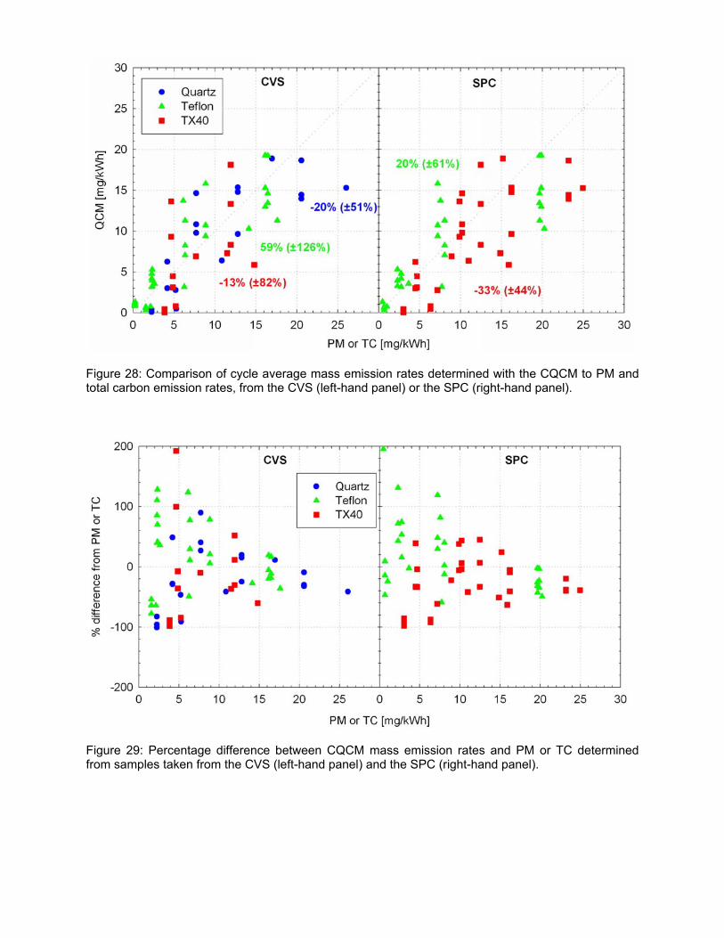
Figure 28: Comparison of cycle average mass emission rates determined with the CQCM to PM and total carbon emission rates, from the CVS (left-hand panel) or the SPC (right-hand panel).

Figure 29: Percentage difference between CQCM mass emission rates and PM or TC determined from samples taken from the CVS (left-hand panel) and the SPC (right-hand panel).

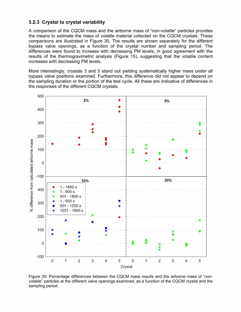
3.2.3 Crystal to crystal variability

A comparison of the CQCM mass and the airborne mass of “non-volatile” particles provides the means to estimate the mass of volatile material collected on the CQCM crystals. These comparisons are illustrated in Figure 30. The results are shown separately for the different bypass valve openings, as a function of the crystal number and sampling period. The differences were found to increase with decreasing PM levels, in good agreement with the results of the thermogravimetric analysis (Figure 15), suggesting that the volatile content increases with decreasing PM levels.

More interestingly, crystals 3 and 5 stand out yielding systematically higher mass under all bypass valve positions examined. Furthermore, this difference did not appear to depend on the sampling duration or the portion of the test cycle. All these are indicative of differences in the responses of the different CQCM crystals.

Figure 30: Percentage differences between the CQCM mass results and the airborne mass of “non-volatile” particles at the different valve openings examined, as a function of the CQCM crystal and the sampling period.

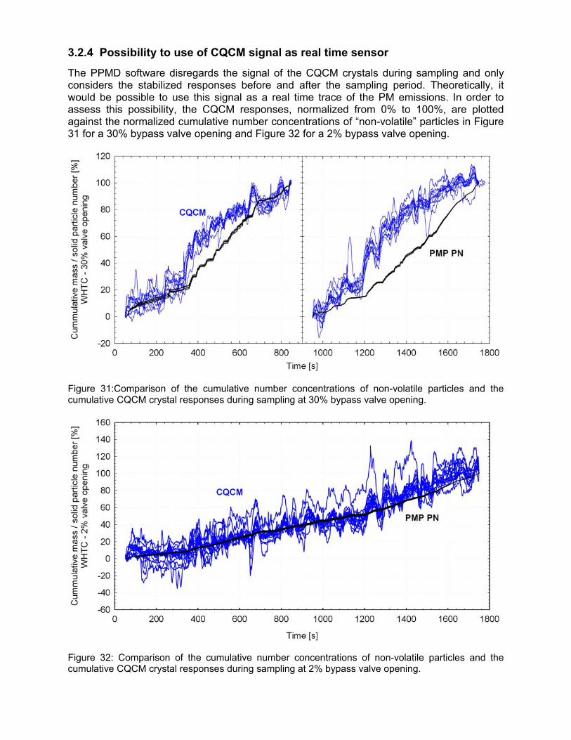
3.2.4 Possibility to use of CQCM signal as real time sensor

The PPMD software disregards the signal of the CQCM crystals during sampling and only considers the stabilized responses before and after the sampling period. Theoretically, it would be possible to use this signal as a real time trace of the PM emissions. In order to assess this possibility, the CQCM responses, normalized from 0% to 100%, are plotted against the normalized cumulative number concentrations of “non-volatile” particles in Figure 31 for a 30% bypass valve opening and Figure 32 for a 2% bypass valve opening.

Figure 31:Comparison of the cumulative number concentrations of non-volatile particles and the cumulative CQCM crystal responses during sampling at 30% bypass valve opening.

Figure 32: Comparison of the cumulative number concentrations of non-volatile particles and the cumulative CQCM crystal responses during sampling at 2% bypass valve opening.

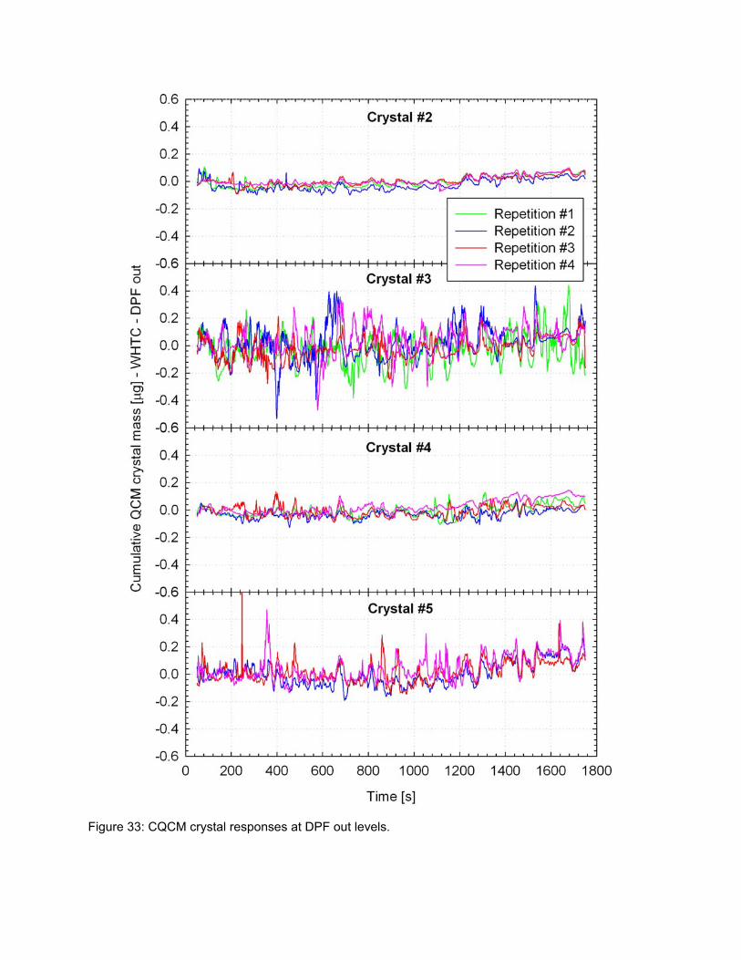
Figure 33: CQCM crystal responses at DPF out levels.

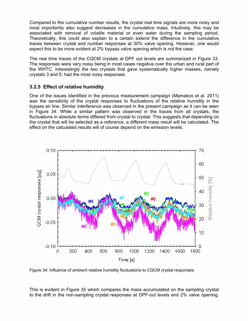
Compared to the cumulative number results, the crystal real time signals are more noisy and most importantly also suggest decreases in the cumulative mass. Intuitively, this may be associated with removal of volatile material or even water during the sampling period. Theoretically, this could also explain to a certain extend the difference in the cumulative traces between crystal and number responses at 30% valve opening. However, one would expect this to be more evident at 2% bypass valve opening which is not the case.

The real time traces of the CQCM crystals at DPF out levels are summarized in Figure 33. The responses were very noisy being in most cases negative over the urban and rural part of the WHTC. Interestingly the two crystals that gave systematically higher masses, namely crystals 3 and 5, had the most noisy responses.

3.2.5 Effect of relative humidity

One of the issues identified in the previous measurement campaign (Mamakos et al. 2011) was the sensitivity of the crystal responses to fluctuations of the relative humidity in the bypass air line. Similar interference was observed in the present campaign as it can be seen in Figure 34. While a similar pattern was observed in the traces from all crystals, the fluctuations in absolute terms differed from crystal to crystal. This suggests that depending on the crystal that will be selected as a reference, a different mass result will be calculated. The effect on the calculated results will of course depend on the emission levels.

Figure 34: Influence of ambient relative humidity fluctuations to CQCM crystal responses.

This is evident in Figure 35 which compares the mass accumulated on the sampling crystal to the drift in the non-sampling crystal responses at DPF-out levels and 2% valve opening.

Depending on the crystal selected as a reference, the accumulated CQCM mass can be anywhere between 0.053 and 0.123 ug at DPF out levels. This introduces a 35% uncertainty in the calculated mass at these levels. The effect becomes less pronounced at 2% bypass valve opening where the choice of reference crystal introduces an uncertainty of only 4% in the calculated crystal mass (0.414 to 0.459 ug).

Figure 35: Comparison of the mass accumulated on the sampling crystal to the drift in the signals of the non-sampling crystals, at DPF out levels (upper panel) and 2% bypass valve opening (lower panel).

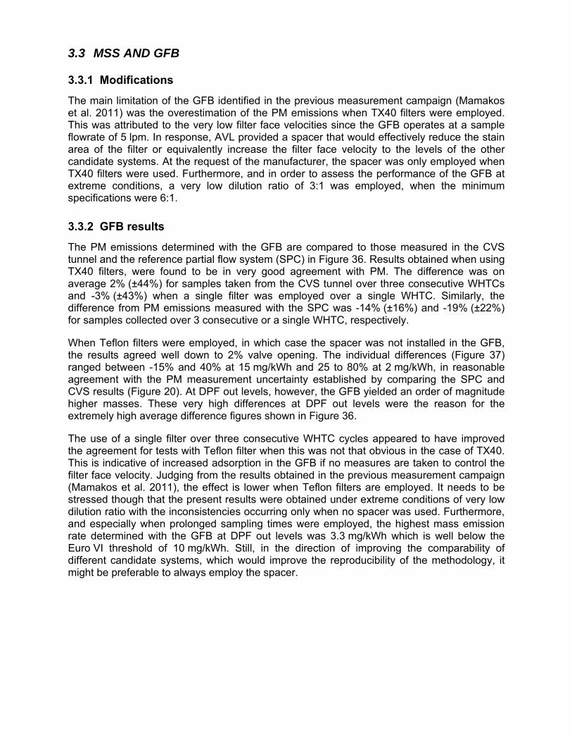
3.3 MSS AND GFB

3.3.1 Modifications

The main limitation of the GFB identified in the previous measurement campaign (Mamakos et al. 2011) was the overestimation of the PM emissions when TX40 filters were employed. This was attributed to the very low filter face velocities since the GFB operates at a sample flowrate of 5 lpm. In response, AVL provided a spacer that would effectively reduce the stain area of the filter or equivalently increase the filter face velocity to the levels of the other candidate systems. At the request of the manufacturer, the spacer was only employed when TX40 filters were used. Furthermore, and in order to assess the performance of the GFB at extreme conditions, a very low dilution ratio of 3:1 was employed, when the minimum specifications were 6:1.

3.3.2 GFB results

The PM emissions determined with the GFB are compared to those measured in the CVS tunnel and the reference partial flow system (SPC) in Figure 36. Results obtained when using TX40 filters, were found to be in very good agreement with PM. The difference was on average 2% (±44%) for samples taken from the CVS tunnel over three consecutive WHTCs and -3% (±43%) when a single filter was employed over a single WHTC. Similarly, the difference from PM emissions measured with the SPC was -14% (±16%) and -19% (±22%) for samples collected over 3 consecutive or a single WHTC, respectively.

When Teflon filters were employed, in which case the spacer was not installed in the GFB, the results agreed well down to 2% valve opening. The individual differences (Figure 37) ranged between -15% and 40% at 15 mg/kWh and 25 to 80% at 2 mg/kWh, in reasonable agreement with the PM measurement uncertainty established by comparing the SPC and CVS results (Figure 20). At DPF out levels, however, the GFB yielded an order of magnitude higher masses. These very high differences at DPF out levels were the reason for the extremely high average difference figures shown in Figure 36.

The use of a single filter over three consecutive WHTC cycles appeared to have improved the agreement for tests with Teflon filter when this was not that obvious in the case of TX40. This is indicative of increased adsorption in the GFB if no measures are taken to control the filter face velocity. Judging from the results obtained in the previous measurement campaign (Mamakos et al. 2011), the effect is lower when Teflon filters are employed. It needs to be stressed though that the present results were obtained under extreme conditions of very low dilution ratio with the inconsistencies occurring only when no spacer was used. Furthermore, and especially when prolonged sampling times were employed, the highest mass emission rate determined with the GFB at DPF out levels was 3.3 mg/kWh which is well below the Euro VI threshold of 10 mg/kWh. Still, in the direction of improving the comparability of different candidate systems, which would improve the reproducibility of the methodology, it might be preferable to always employ the spacer.

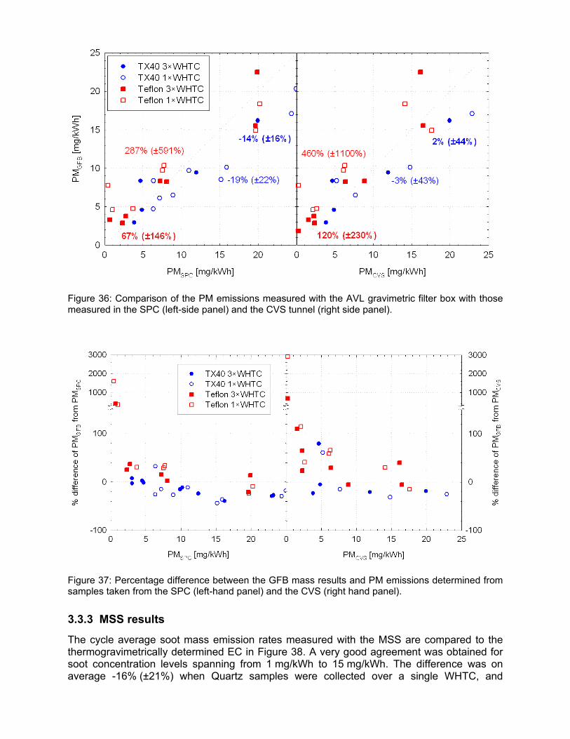
Figure 36: Comparison of the PM emissions measured with the AVL gravimetric filter box with those measured in the SPC (left-side panel) and the CVS tunnel (right side panel).

Figure 37: Percentage difference between the GFB mass results and PM emissions determined from samples taken from the SPC (left-hand panel) and the CVS (right hand panel).

3.3.3 MSS results

The cycle average soot mass emission rates measured with the MSS are compared to the thermogravimetrically determined EC in Figure 38. A very good agreement was obtained for soot concentration levels spanning from 1 mg/kWh to 15 mg/kWh. The difference was on average -16% (±21%) when Quartz samples were collected over a single WHTC, and

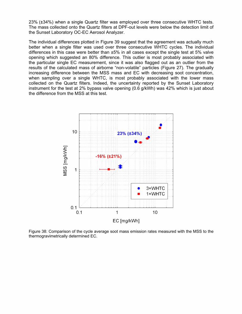
23% (±34%) when a single Quartz filter was employed over three consecutive WHTC tests. The mass collected onto the Quartz filters at DPF-out levels were below the detection limit of the Sunset Laboratory OC-EC Aerosol Analyzer.

The individual differences plotted in Figure 39 suggest that the agreement was actually much better when a single filter was used over three consecutive WHTC cycles. The individual differences in this case were better than ±5% in all cases except the single test at 5% valve opening which suggested an 80% difference. This outlier is most probably associated with the particular single EC measurement, since it was also flagged out as an outlier from the results of the calculated mass of airborne “non-volatile” particles (Figure 27). The gradually increasing difference between the MSS mass and EC with decreasing soot concentration, when sampling over a single WHTC, is most probably associated with the lower mass collected on the Quartz filters. Indeed, the uncertainty reported by the Sunset Laboratory instrument for the test at 2% bypass valve opening (0.6 g/kWh) was 42% which is just about the difference from the MSS at this test.

Figure 38: Comparison of the cycle average soot mass emission rates measured with the MSS to the thermogravimetrically determined EC.

Figure 39: Percentage differences between the soot mass determined with the MSS and the thermogravimetrically determined EC.

The MSS responses were also found to be in good agreement with the calculated mass of airborne particles as can be seen in Figure 40. The difference was on average 14% (±9%) at emission levels spanning from 1 to 15 mg/kWh. At DPF out levels, the MSS response was measuring around 0.05 mg/kWh. This figure was 400% higher from the mass calculated from the SPCS results which were already overestimating the true emission levels due to the high background (Figure 22). Therefore, it can be concluded that the lower detection limit for the MSS was 0.05 mg/kWh (~5 ug/m3), for the exhaust of the particular engine. These values are almost an order of magnitude lower from the detection limit of 0.3 mg/kWh determined in the previous campaign (Mamakos et al. 2011).

Figure 41 compares the results obtained with the two MSS employed in the study. Again, a very good agreement was observed at emission levels above 1 mg/kWh with the difference being on average 4% (±7%). At DPF-out levels, the two MSS units differed by 51% (±7%), with the JRC owned MSS measuring higher levels (~0.1 mg/kWh). This is in the opposite direction of what was found in the previous campaign where at DPF out levels, the JRC owned MSS was measuring lower (Mamakos et al. 2011).

An examination of the gaseous emissions can give some further insight on the reason for the differences between the two measurement campaigns. This issue is discussed in more details in section 3.3.3.1.

The real time responses of the MSS are compared with the real time mass of airborne “non-volatile” particles in Figure 42. A reasonable agreement was observed down to 2% bypass valve opening, but at DPF out levels the MSS response was at least an order of magnitude higher from what expected from the measured number counts.

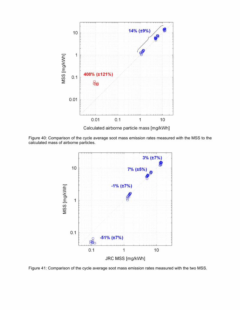
Figure 40: Comparison of the cycle average soot mass emission rates measured with the MSS to the calculated mass of airborne particles.

Figure 41: Comparison of the cycle average soot mass emission rates measured with the two MSS.

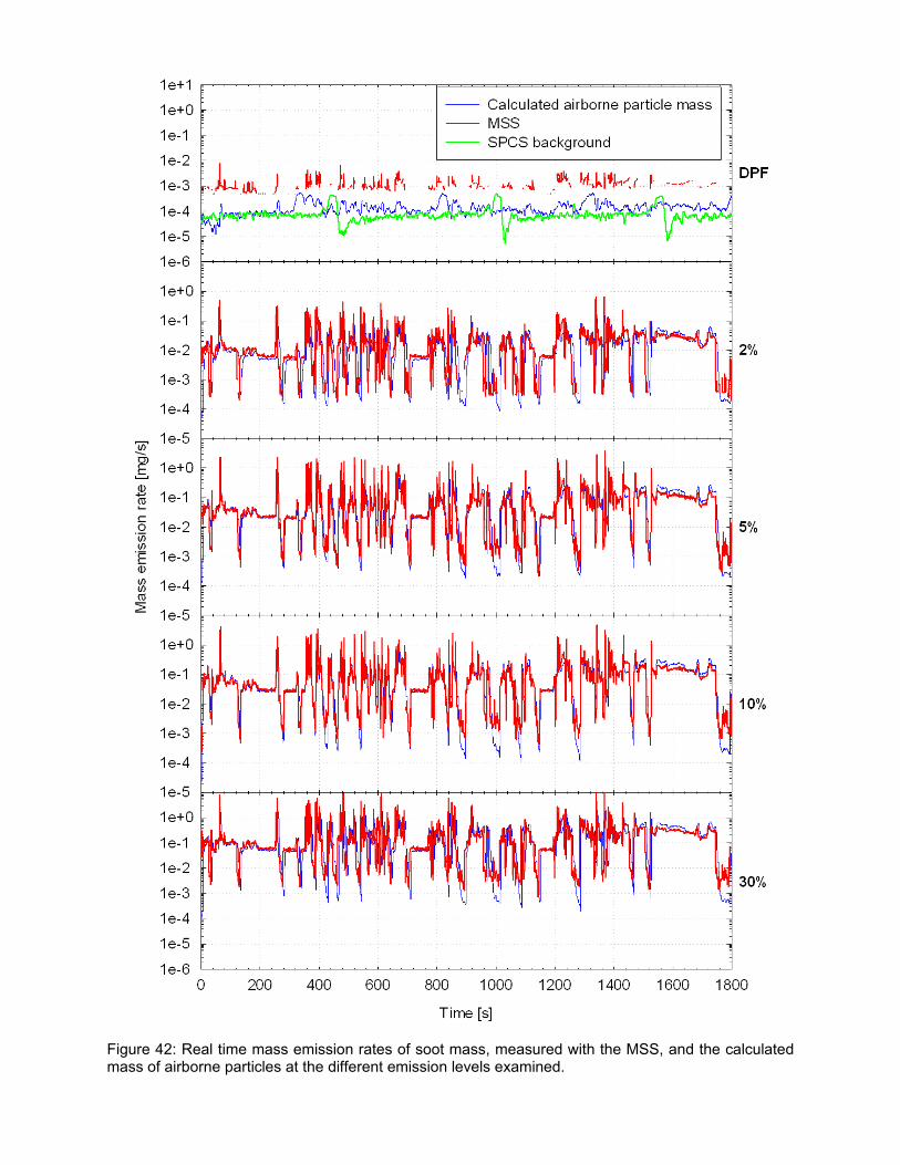
Figure 42: Real time mass emission rates of soot mass, measured with the MSS, and the calculated mass of airborne particles at the different emission levels examined.

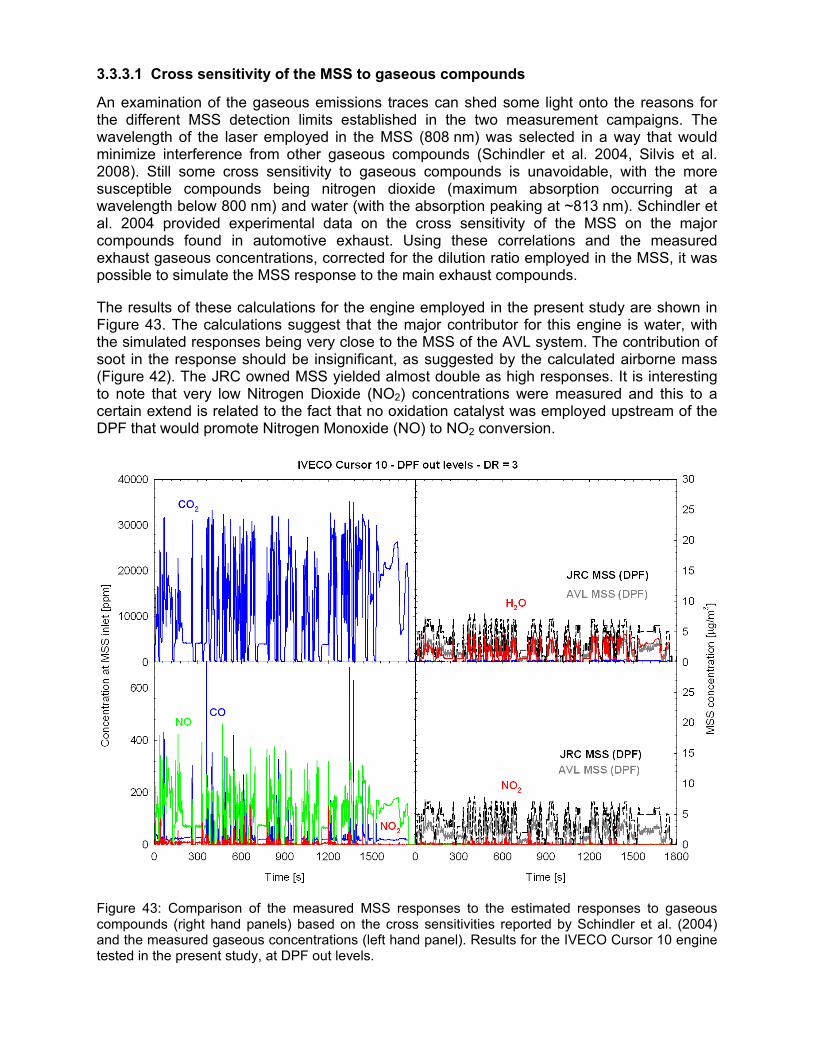
3.3.3.1 Cross sensitivity of the MSS to gaseous compounds

An examination of the gaseous emissions traces can shed some light onto the reasons for the different MSS detection limits established in the two measurement campaigns. The wavelength of the laser employed in the MSS (808 nm) was selected in a way that would minimize interference from other gaseous compounds (Schindler et al. 2004, Silvis et al. 2008). Still some cross sensitivity to gaseous compounds is unavoidable, with the more susceptible compounds being nitrogen dioxide (maximum absorption occurring at a wavelength below 800 nm) and water (with the absorption peaking at ~813 nm). Schindler et al. 2004 provided experimental data on the cross sensitivity of the MSS on the major compounds found in automotive exhaust. Using these correlations and the measured exhaust gaseous concentrations, corrected for the dilution ratio employed in the MSS, it was possible to simulate the MSS response to the main exhaust compounds.

The results of these calculations for the engine employed in the present study are shown in Figure 43. The calculations suggest that the major contributor for this engine is water, with the simulated responses being very close to the MSS of the AVL system. The contribution of soot in the response should be insignificant, as suggested by the calculated airborne mass (Figure 42). The JRC owned MSS yielded almost double as high responses. It is interesting to note that very low Nitrogen Dioxide (NO2) concentrations were measured and this to a certain extend is related to the fact that no oxidation catalyst was employed upstream of the DPF that would promote Nitrogen Monoxide (NO) to NO2 conversion.

Figure 43: Comparison of the measured MSS responses to the estimated responses to gaseous compounds (right hand panels) based on the cross sensitivities reported by Schindler et al. (2004) and the measured gaseous concentrations (left hand panel). Results for the IVECO Cursor 10 engine tested in the present study, at DPF out levels.

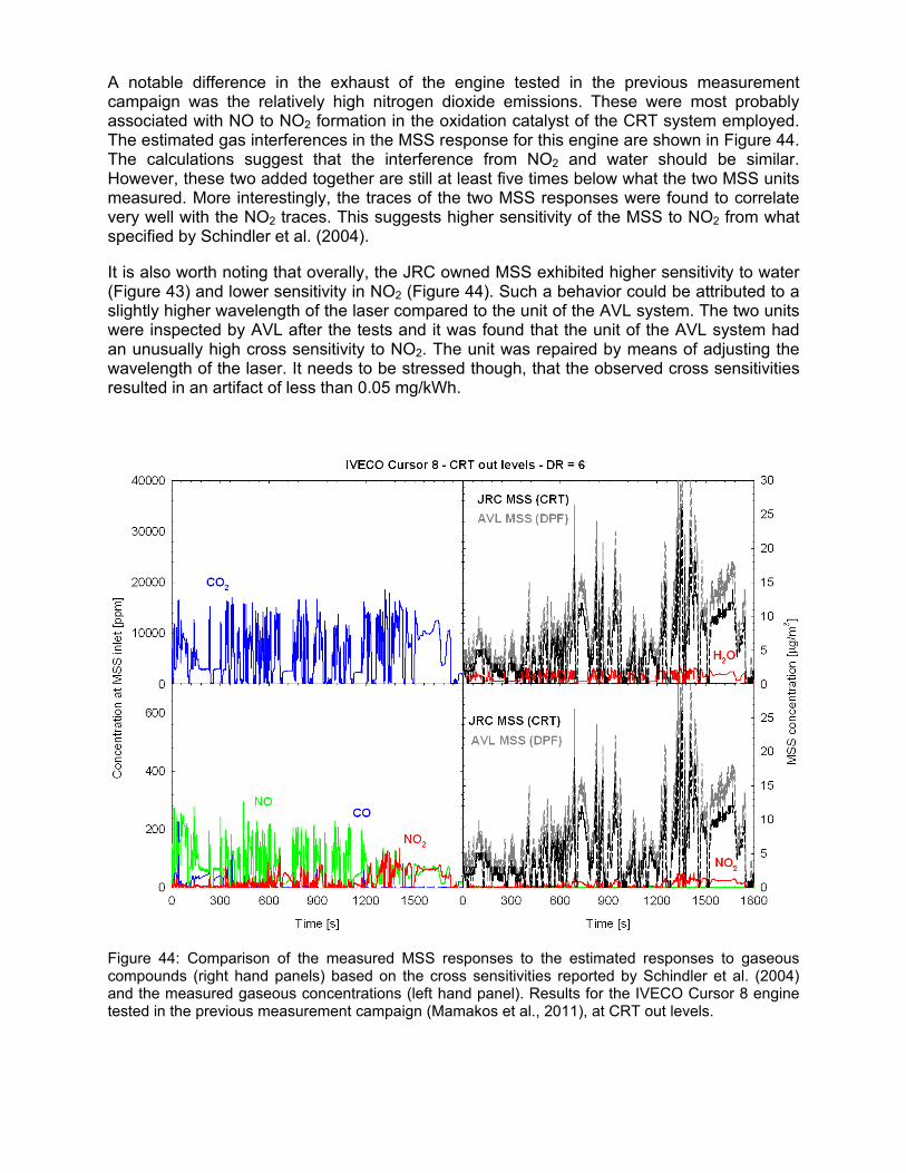
A notable difference in the exhaust of the engine tested in the previous measurement campaign was the relatively high nitrogen dioxide emissions. These were most probably associated with NO to NO2 formation in the oxidation catalyst of the CRT system employed. The estimated gas interferences in the MSS response for this engine are shown in Figure 44. The calculations suggest that the interference from NO2 and water should be similar. However, these two added together are still at least five times below what the two MSS units measured. More interestingly, the traces of the two MSS responses were found to correlate very well with the NO2 traces. This suggests higher sensitivity of the MSS to NO2 from what specified by Schindler et al. (2004).

It is also worth noting that overally, the JRC owned MSS exhibited higher sensitivity to water (Figure 43) and lower sensitivity in NO2 (Figure 44). Such a behavior could be attributed to a slightly higher wavelength of the laser compared to the unit of the AVL system. The two units were inspected by AVL after the tests and it was found that the unit of the AVL system had an unusually high cross sensitivity to NO2. The unit was repaired by means of adjusting the wavelength of the laser. It needs to be stressed though, that the observed cross sensitivities resulted in an artifact of less than 0.05 mg/kWh.

Figure 44: Comparison of the measured MSS responses to the estimated responses to gaseous compounds (right hand panels) based on the cross sensitivities reported by Schindler et al. (2004) and the measured gaseous concentrations (left hand panel). Results for the IVECO Cursor 8 engine tested in the previous measurement campaign (Mamakos et al., 2011), at CRT out levels.

3.4 DMM

3.4.1 Modifications

No modifications were envisaged for the DMM by the manufacturer in the present campaign. The results from the previous campaign suggested that no thermal treatment of the aerosol is required, and therefore all tests were performed with the DMM sampling directly from the CVS. Special care was taken to thoroughly clean the impactors at the end of each measuring day.

3.4.2 Correlation with EC and mass of airborne “non-volatile” particles

The operation principle of the DMM is based on the determination of the effective particle density by comparing aerodynamic (impactor stages) and mobility diameters (mobility diameters). Therefore its response relates to the mass of all airborne particles, including volatile and “non-volatile”. Figure 45 compares the mass calculated with the DMM to the EC and the calculated mass of airborne “non-volatile” particles. A very good agreement was observed in both cases, the difference being on average 7% (±32%) from EC and -15% (±10%) from the calculated “non-volatile” airborne mass.

The above figures did not take into account some experimental data, shown as empty symbols in the chart, for which it is suspected that there was a leak in the system. This was identified at the end of a measurement day by measurement of the sample flowrate, which was found to be lower from its nominal value (~6 lpm instead of ~9 lpm). This leak was related to the sealing of the sheath air line, inside the instrument. While the particular measurements were disregarded, it is expected that some leak also occurred in some earlier measurements, where the DMM yielded similarly lower mass emissions. It needs to be stressed that the particular problem would have been identified with the leakage checks suggested by the manufacturer, which however were not performed in the particular campaign.

The individual differences (Figure 46) suggest that with the exception of the measurements at DPF-out levels where (as it will be shown latter) the DMM had reached its detection limit and the single EC result that was signed out as an outlier from all instruments, the DMM yielded systematically lower masses by ~20%. This is intuitively wrong, in the sense that DMM also measures the total airborne particle population (including volatile particles) and should therefore yield higher or at least similar results. An examination of the particle number concentrations measured by the instrument (section 3.4.3) can give some insight on the reason for this inconsistency.

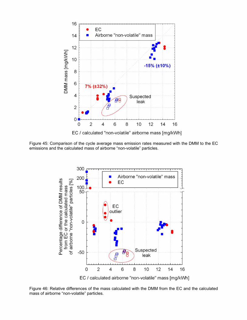
Figure 45: Comparison of the cycle average mass emission rates measured with the DMM to the EC emissions and the calculated mass of airborne “non-volatile” particles.

Figure 46: Relative differences of the mass calculated with the DMM from the EC and the calculated mass of airborne “non-volatile” particles.

3.4.3 Number results

Figure 47 compares the number emission rates of the total particle population measured with the DMM to those of the “non-volatile” particles measured with the PMP-compliant system. The DMM has a lower aerodynamic cut-off size at 29.6 nm, which for the effective density profile assumed (Figure 25) corresponds to a mobility diameter of approximately 23 nm. This is actually the cut-off size of the CPC used in the SPCS and therefore the results should be comparable.

The DMM was found to yield systematically higher number emissions, with the difference averaging at 103% (±28%). This may be due to the presence of volatile nucleation mode particles that are not counted by the SPCS. However this is not verified by the DMM impactor responses which rather suggest a mono-modal distribution (Figure 47 – right hand panel).

Maricq et al. (2006) employed a similar methodology to an Electrical Low Pressure Impactor. They found that this approach is quite robust in the determination of the airborne particle mass since an underestimation of the particle size results in an overestimation of their number concentration and vice versa. The calibration experiments conducted in the previous measurement campaign (Mamakos et al. 2011) yielded larger cut-off sizes from the nominal values employed in the software. It is therefore expected that the software underestimates somehow the particle size and therefore the associated charger efficiency. This can lead to an overestimation of the number concentration, in line with what the DMM – SPCS comparisons showed. Furthermore, the calibration experiments also suggested an underestimation of the true charger efficiency which also directly translates to an overestimation of the number concentrations. It should be stressed however, that even with such a large overestimation of the number concentrations, a modest effect was observed in the calculated mass results, in good agreement with what Maricq et al. (2006) suggested.

Figure 47: Comparison of number emission rates of total particles measured with the DMM to those of “non-volatile” particles measured with the SPCS (left-hand panel). The figure on the right shows the cycle average distributions of impactor currents for one example WHTC test.

3.4.4 Real time responses

Figure 48 compares the real time mass emission rates measured with the DMM to the real time mass of airborne “non-volatile” particles calculated from the SPCS signals. In good agreement with the results of the previous campaign, the detection limit of the DMM was found to be around 0.3 ug/m3. This figure was above the emitted concentrations at DPF-out levels where the DMM response was relatively flat and very noisy.

Above this level, however, the real time traces of the DMM mass results were closely following the calculated mass emission rates from the SPCS. In absolute terms, the DMM yielded systematically lower mass over the whole test cycle. This reinforces the intuition that the DMM underestimates the airborne mass due to errors in the cut-off sizes employed in the software.

Figure 48: Real time mass emission rates of the total particle population measured with the DMM and the “non-volatile” particles calculated from the SPCS responses.

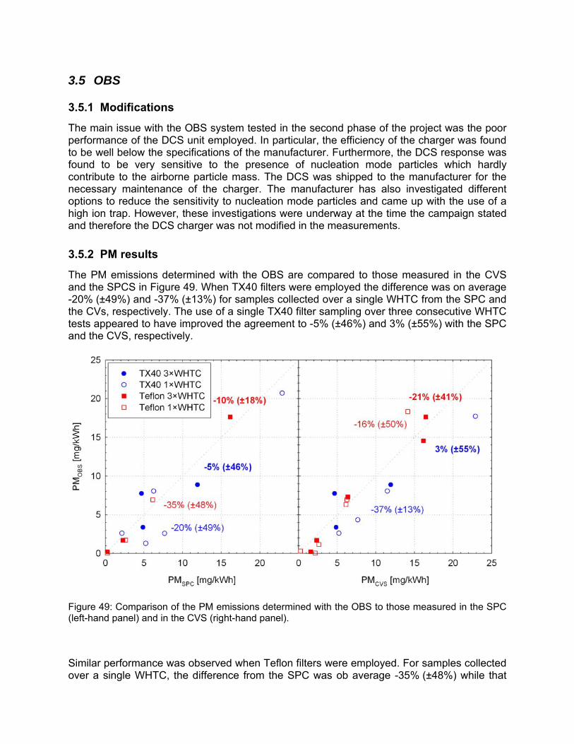
3.5 OBS

3.5.1 Modifications

The main issue with the OBS system tested in the second phase of the project was the poor performance of the DCS unit employed. In particular, the efficiency of the charger was found to be well below the specifications of the manufacturer. Furthermore, the DCS response was found to be very sensitive to the presence of nucleation mode particles which hardly contribute to the airborne particle mass. The DCS was shipped to the manufacturer for the necessary maintenance of the charger. The manufacturer has also investigated different options to reduce the sensitivity to nucleation mode particles and came up with the use of a high ion trap. However, these investigations were underway at the time the campaign stated and therefore the DCS charger was not modified in the measurements.

3.5.2 PM results

The PM emissions determined with the OBS are compared to those measured in the CVS and the SPCS in Figure 49. When TX40 filters were employed the difference was on average -20% (±49%) and -37% (±13%) for samples collected over a single WHTC from the SPC and the CVs, respectively. The use of a single TX40 filter sampling over three consecutive WHTC tests appeared to have improved the agreement to -5% (±46%) and 3% (±55%) with the SPC and the CVS, respectively.

Figure 49: Comparison of the PM emissions determined with the OBS to those measured in the SPC (left-hand panel) and in the CVS (right-hand panel).

Similar performance was observed when Teflon filters were employed. For samples collected over a single WHTC, the difference from the SPC was ob average -35% (±48%) while that

from the CVS averaged at -16% (±50%). The use of a single filter over three consecutive WHTC tests resulted in an average difference of -10% (±18%) from the SPC and -21% (±41%) from the CVS.

Figure 50 shows the individual differences of the OBS results from the PM determined from samples taken from the SPC (left-hand panel) and the CVS (right-hand panel). The relative differences increased with decreasing PM levels from approximately ±40% at 10 mg/kWh to ±100% at DPF out levels. These figures compare well to the differences observed between the SPC and the CVS, suggesting equivalent performance of the OBS.

Figure 50: Percentage difference between the PM emissions determined with the OBS and the PM emissions determined from samples taken from the SPC (left-hand panel) and the CVS (right hand panel).

3.5.3 DCS calibration

Some checks performed upon receipt of the DCS following its maintenance, suggested that the charger was still not working properly. These checks consisted of measuring the current produced from the charger by means of turning off the trap voltage. The ion current should be around 40 to 60 pA, depending on the ambient conditions, but the tests yielded consistently lower values ranging from 30 to 37 pA. However, due to time constraints it was not possible to send the instrument to the manufacturer for further checks. The ion current was measured regularly during the measurement campaign and was always found to be below the specified operating range and was not constant throughout the measurement day.

The lower ion concentration produced by the charger effectively results in a lower charging efficiency, which translates to a lower measured signal (current) for a given aerosol concentration. Some calibration experiments conducted at the end of the measurements campaign employing graphite particles (Figure 14a) verified the low charger efficiency of the DCS. The ion current measured before the calibration experiments was found to be 27 pA.

Figure 51 compares the results of these experiments to those performed with PAO particles before shipping the DCS and the nominal charging efficiency. Even if the efficiency of the charger improved after the maintenance of the unit, it was still approximately half the nominal value. This deterioration of the charger performance did not affect the slope of the DCS response which for the case of neutralized particles was found to be 1.07, very close to the nominal value of 1.133. The DCS was found to exhibit a slightly higher efficiency for singly charged particles but the actual difference (~5 to 10%) was very low to allow for definite conclusions.

Figure 51: Comparison of the experimentally determined charging efficiency of the DCS with graphite particles (open dots) to those measured with PAO particles before shipping the DCS (filled dots) and the nominal charging efficiency (green line).

3.5.4 DCS responses to engine exhaust

The current measured by the DCS is close to being proportional to the particle diameter (actually proportional to the diameter raised to the power of 1.1). Accordingly, TSI utilizes a proportionality constant of 6.09756 to translate the measured current (in pA) to length concentrations (mm/cm3). If the number concentration is also measured, then the ratio of the length measured by the DCS to the number concentration would yield the length-weighted average particle size. For lognormal distributions, the geometric mean diameter of the qth moment distribution (qMD) is related to the count mean diameter (that coincides with the geometric mean diameter dg) through (Hinds W. C. 1999):

( )[ ]gg qdqMD σ2lnexp= 4

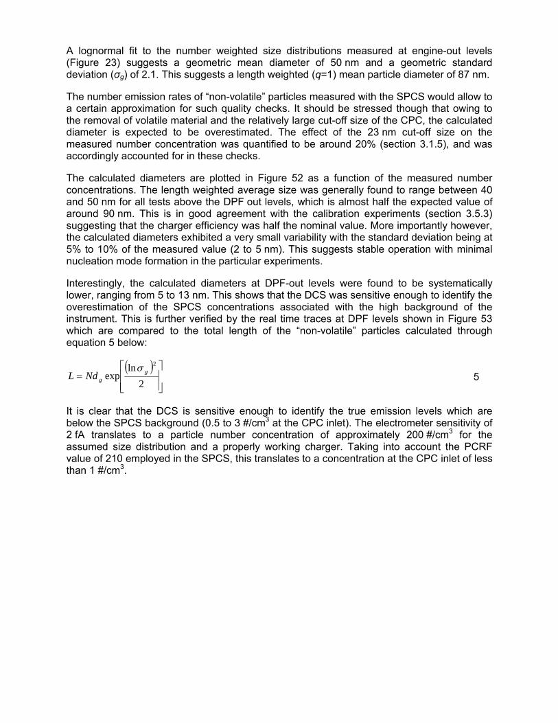
A lognormal fit to the number weighted size distributions measured at engine-out levels (Figure 23) suggests a geometric mean diameter of 50 nm and a geometric standard deviation (σg) of 2.1. This suggests a length weighted (q=1) mean particle diameter of 87 nm.

The number emission rates of “non-volatile” particles measured with the SPCS would allow to a certain approximation for such quality checks. It should be stressed though that owing to the removal of volatile material and the relatively large cut-off size of the CPC, the calculated diameter is expected to be overestimated. The effect of the 23 nm cut-off size on the measured number concentration was quantified to be around 20% (section 3.1.5), and was accordingly accounted for in these checks.

The calculated diameters are plotted in Figure 52 as a function of the measured number concentrations. The length weighted average size was generally found to range between 40 and 50 nm for all tests above the DPF out levels, which is almost half the expected value of around 90 nm. This is in good agreement with the calibration experiments (section 3.5.3) suggesting that the charger efficiency was half the nominal value. More importantly however, the calculated diameters exhibited a very small variability with the standard deviation being at 5% to 10% of the measured value (2 to 5 nm). This suggests stable operation with minimal nucleation mode formation in the particular experiments.

Interestingly, the calculated diameters at DPF-out levels were found to be systematically lower, ranging from 5 to 13 nm. This shows that the DCS was sensitive enough to identify the overestimation of the SPCS concentrations associated with the high background of the instrument. This is further verified by the real time traces at DPF levels shown in Figure 53 which are compared to the total length of the “non-volatile” particles calculated through equation 5 below:

( )⎥⎥⎦

⎤

⎢⎢⎣

⎡=

2ln

exp2

ggNdL

σ 5

It is clear that the DCS is sensitive enough to identify the true emission levels which are below the SPCS background (0.5 to 3 #/cm3 at the CPC inlet). The electrometer sensitivity of 2 fA translates to a particle number concentration of approximately 200 #/cm3 for the assumed size distribution and a properly working charger. Taking into account the PCRF value of 210 employed in the SPCS, this translates to a concentration at the CPC inlet of less than 1 #/cm3.

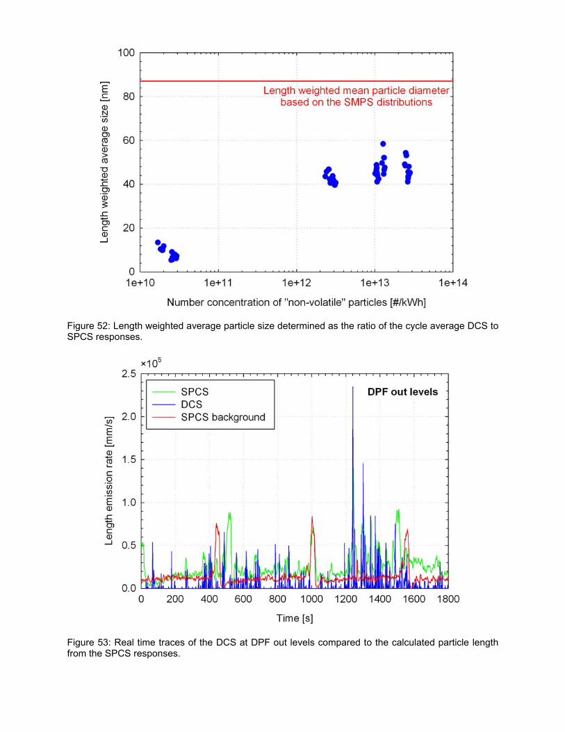
Figure 52: Length weighted average particle size determined as the ratio of the cycle average DCS to SPCS responses.

Figure 53: Real time traces of the DCS at DPF out levels compared to the calculated particle length from the SPCS responses.

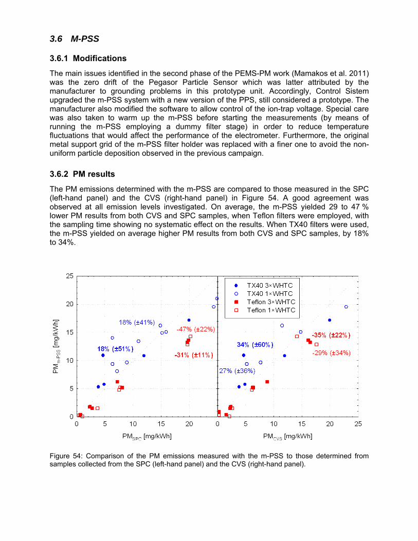
3.6 M-PSS

3.6.1 Modifications

The main issues identified in the second phase of the PEMS-PM work (Mamakos et al. 2011) was the zero drift of the Pegasor Particle Sensor which was latter attributed by the manufacturer to grounding problems in this prototype unit. Accordingly, Control Sistem upgraded the m-PSS system with a new version of the PPS, still considered a prototype. The manufacturer also modified the software to allow control of the ion-trap voltage. Special care was also taken to warm up the m-PSS before starting the measurements (by means of running the m-PSS employing a dummy filter stage) in order to reduce temperature fluctuations that would affect the performance of the electrometer. Furthermore, the original metal support grid of the m-PSS filter holder was replaced with a finer one to avoid the non-uniform particle deposition observed in the previous campaign.

3.6.2 PM results

The PM emissions determined with the m-PSS are compared to those measured in the SPC (left-hand panel) and the CVS (right-hand panel) in Figure 54. A good agreement was observed at all emission levels investigated. On average, the m-PSS yielded 29 to 47 % lower PM results from both CVS and SPC samples, when Teflon filters were employed, with the sampling time showing no systematic effect on the results. When TX40 filters were used, the m-PSS yielded on average higher PM results from both CVS and SPC samples, by 18% to 34%.

Figure 54: Comparison of the PM emissions measured with the m-PSS to those determined from samples collected from the SPC (left-hand panel) and the CVS (right-hand panel).

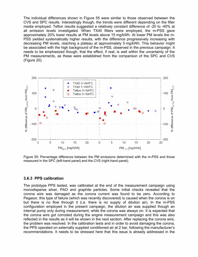
The individual differences shown in Figure 55 were similar to those observed between the CVS and SPC results. Interestingly though, the trends were different depending on the filter media employed. Teflon results suggested a relatively constant difference of -20 to -40% at all emission levels investigated. When TX40 filters were employed, the m-PSS gave approximately 20% lower results at PM levels above 15 mg/kWh. At lower PM levels the m-PSS yielded systematically higher results, with the difference progressively increasing with decreasing PM levels, reaching a plateau at approximately 5 mg/kWh. This behavior might be associated with the high background of the m-PSS, observed in the previous campaign. It needs to be emphasized though, that the effect, if real, is well within the uncertainty of the PM measurements, as these were established from the comparison of the SPC and CVS (Figure 20).

Figure 55: Percentage difference between the PM emissions determined with the m-PSS and those measured in the SPC (left-hand panel) and the CVS (right-hand panel).

3.6.3 PPS calibration

The prototype PPS tested, was calibrated at the end of the measurement campaign using monodisperse silver, PAO and graphite particles. Some initial checks revealed that the corona wire was damaged as the corona current was found to be zero. According to Pegasor, this type of failure (which was recently discovered) is caused when the corona is on but there is no flow through it (i.e. there is no supply of dilution air). In the m-PSS configuration employed in the present campaign, the dilution air was supplied though an internal pump only during measurement, while the corona was always on. It is expected that the corona wire got corroded during the engine measurement campaign and this was also reflected in the results as it will be shown in the next section. After replacing the corona wire, the problem was resolved. In the calibration tests and in order to avoid damaging the corona, the PPS operated on externally supplied conditioned air at 2 bar, following the manufacturer’s recommendations. It needs to be stressed here that this issue is already addressed in the

current version of the m-PSS, where the corona voltage is only applied when there is a flow of dilution air.

3.6.3.1 Charger efficiency

The PPS unit tested appeared to have also some zero drift problems. The zero levels of the sensor were found to be very unstable in all tests performed even after several hours of continuous operation. As an example, Figure 56 shows typical recordings of PPS Particle Sensor and the 3025A CPC for calibration tests with neutralized graphite particles. It can be seen that the zero levels of the PPS (i.e. the indications when a zero voltage was applied on the DMA) varied significantly during this 75 min testing. Note that the relatively long time required for the CPC indication to drop to zero is related to the relatively large volume of the neutralizer (time required to purge the aerosol from the neutralizer). This drift of the electrometer zero level resulted in relatively large uncertainties in the calculated charger efficiencies. This was particularly true in the case of PAO particles due to the relatively lower concentrations. In order to quantify this effect, two charger efficiencies were calculated (and reported) at each voltage setting, one using the zero levels recorded before and one using the zero levels recorded after the actual measurement.

Figure 56: Responses of the PPS and the 3025 CPC for the calibration of neutralized graphite particles at 50 V trap voltage.

The performance of corona chargers is characterized by the charger efficiency (β), which is the quantity relating the total charge acquired by particles of a given size and their number concentration, i.e.:

( )[ ] ( )[ ] ( ) ⎥⎦⎤

⎢⎣⎡= 3

3 #cm

dNfAcmdfAdI BBB β 6

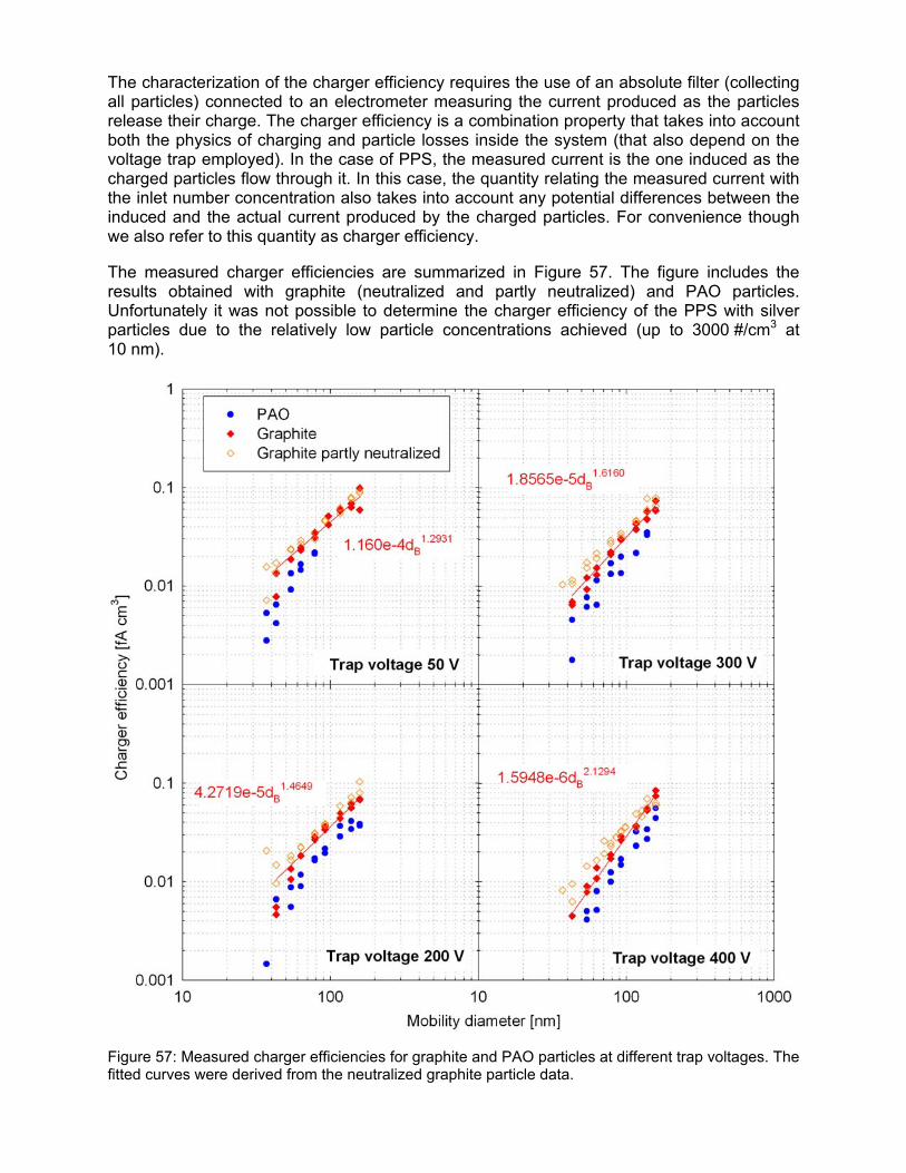
The characterization of the charger efficiency requires the use of an absolute filter (collecting all particles) connected to an electrometer measuring the current produced as the particles release their charge. The charger efficiency is a combination property that takes into account both the physics of charging and particle losses inside the system (that also depend on the voltage trap employed). In the case of PPS, the measured current is the one induced as the charged particles flow through it. In this case, the quantity relating the measured current with the inlet number concentration also takes into account any potential differences between the induced and the actual current produced by the charged particles. For convenience though we also refer to this quantity as charger efficiency.

The measured charger efficiencies are summarized in Figure 57. The figure includes the results obtained with graphite (neutralized and partly neutralized) and PAO particles. Unfortunately it was not possible to determine the charger efficiency of the PPS with silver particles due to the relatively low particle concentrations achieved (up to 3000 #/cm3 at 10 nm).

Figure 57: Measured charger efficiencies for graphite and PAO particles at different trap voltages. The fitted curves were derived from the neutralized graphite particle data.

Focusing on the neutralized graphite particles it can be seen that the use of increased voltage trap results in an apparent increase of the slope of the charger efficiency curve. In that respect, the PPS signal is proportional to the mobility diameter raised to the power of ~1.3 at 50 V trap voltage, while at 400 V trap voltage the PPS signal becomes proportional to the mobility diameter raised to the power of 2.13. The later is very close to the expected dependence of diesel particle mass on the mobility diameter (Maricq et al. 2004).

The tests with partially neutralized graphite particles resulted in slightly higher charger efficiencies at the smallest size range considered with the effect being more pronounced as the trap voltage increased. This is presumably related to the fact that the particular particles already carry more charges than could potentially be acquired in the corona charger of the PPS, and it is physically impossible to reduce their average charge in a unipolar environment.

One very interesting observation was that the tests conducted with spherical PAO particles yielded systematically lower charger efficiencies compared to those performed with graphite particles. The slopes though appear to be similar. Similar differences were observed in tests conducted with other diffusion chargers. It is postulated that this is related to the loose structure of the graphite particles produced by the PALAS generator (Biskos et al. 2004). This issue will be further investigated in the future.

3.6.3.2 Particle penetration

The exact determination of particle penetration through the sensor requires the measurement of the dilution factor which has not been performed. The ratio of upstream to downstream concentration of 160 nm particles (i.e. the largest particle size examined) at 50 V (i.e. the smallest trap voltage investigated) trap voltage was used instead. The resulting particle penetrations (or more precisely the relative penetrations with respect to that of 160 nm particles at 50 V trap voltage) are shown in Figure 58. It can be seen that as the trap voltage increases the particle penetration decreases for all particle sizes. This effectively results in a decrease of the overall sensitivity of the sensor. However, the relative increase of particle losses increase with decreasing particle size. Similar penetrations were obtained for spherical oil droplets and complex graphite aggregates.

Tests with silver particles at sub 20 nm sizes suggest a sudden drop of the particle penetration at these very small sizes. However, there exists a minimum penetration that can be achieved through voltage trap increase at the different sizes (46% at 20 nm and 34 % at 10 nm). Obviously, this corresponds to the fraction of uncharged particles. Once this level is achieved, all charged particles are lost inside the PPS and the uncharged particles exiting the PPS do not produce any signal. This means that by appropriate selection of the ion-trap voltage it is possible to effectively introduce and control a cut-off size.

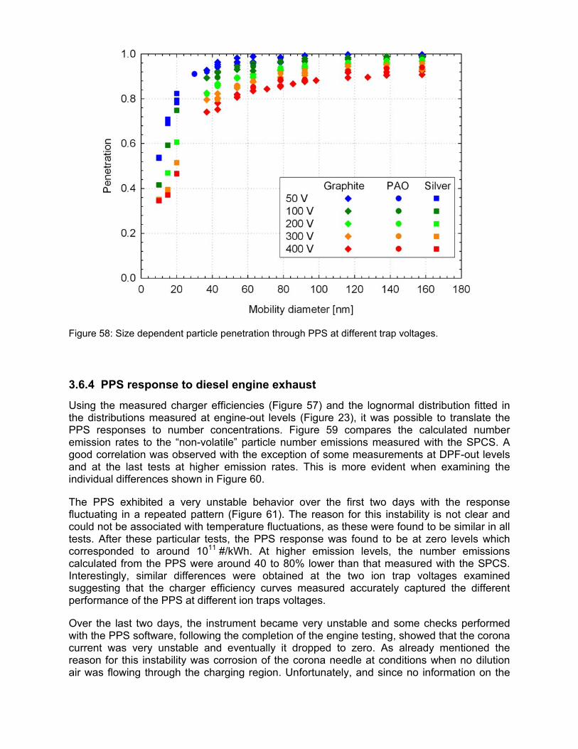
Figure 58: Size dependent particle penetration through PPS at different trap voltages.

3.6.4 PPS response to diesel engine exhaust

Using the measured charger efficiencies (Figure 57) and the lognormal distribution fitted in the distributions measured at engine-out levels (Figure 23), it was possible to translate the PPS responses to number concentrations. Figure 59 compares the calculated number emission rates to the “non-volatile” particle number emissions measured with the SPCS. A good correlation was observed with the exception of some measurements at DPF-out levels and at the last tests at higher emission rates. This is more evident when examining the individual differences shown in Figure 60.

The PPS exhibited a very unstable behavior over the first two days with the response fluctuating in a repeated pattern (Figure 61). The reason for this instability is not clear and could not be associated with temperature fluctuations, as these were found to be similar in all tests. After these particular tests, the PPS response was found to be at zero levels which corresponded to around 1011 #/kWh. At higher emission levels, the number emissions calculated from the PPS were around 40 to 80% lower than that measured with the SPCS. Interestingly, similar differences were obtained at the two ion trap voltages examined suggesting that the charger efficiency curves measured accurately captured the different performance of the PPS at different ion traps voltages.

Over the last two days, the instrument became very unstable and some checks performed with the PPS software, following the completion of the engine testing, showed that the corona current was very unstable and eventually it dropped to zero. As already mentioned the reason for this instability was corrosion of the corona needle at conditions when no dilution air was flowing through the charging region. Unfortunately, and since no information on the

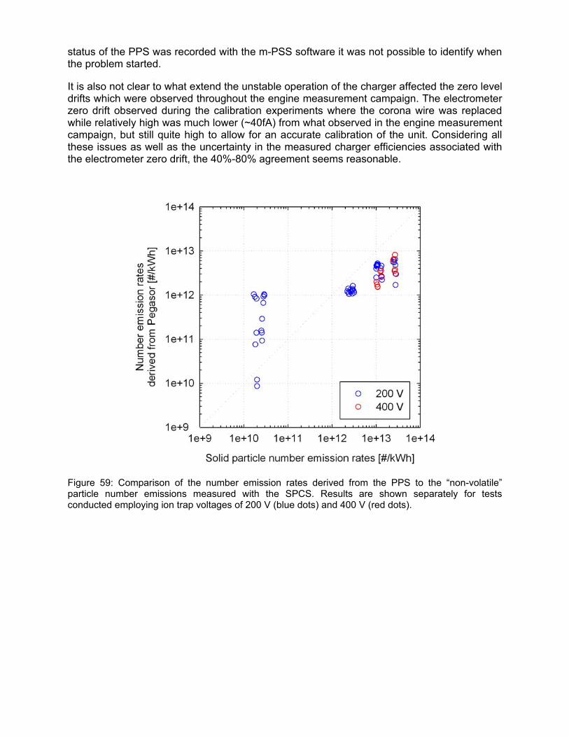
status of the PPS was recorded with the m-PSS software it was not possible to identify when the problem started.

It is also not clear to what extend the unstable operation of the charger affected the zero level drifts which were observed throughout the engine measurement campaign. The electrometer zero drift observed during the calibration experiments where the corona wire was replaced while relatively high was much lower (~40fA) from what observed in the engine measurement campaign, but still quite high to allow for an accurate calibration of the unit. Considering all these issues as well as the uncertainty in the measured charger efficiencies associated with the electrometer zero drift, the 40%-80% agreement seems reasonable.

Figure 59: Comparison of the number emission rates derived from the PPS to the “non-volatile” particle number emissions measured with the SPCS. Results are shown separately for tests conducted employing ion trap voltages of 200 V (blue dots) and 400 V (red dots).

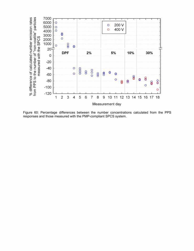
Figure 60: Percentage differences between the number concentrations calculated from the PPS responses and those measured with the PMP-compliant SPCS system.

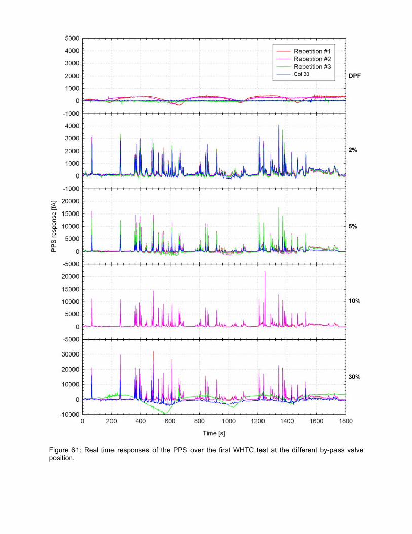
Figure 61: Real time responses of the PPS over the first WHTC test at the different by-pass valve position.

4 CONCLUSIONS This third phase of the PEMS-PM project supplements the second phase campaign with additional investigations at emission levels spanning from Euro V to post DPF using again a bypass/DPF configuration. The main focus of the study was to investigate the effect of sampling time on the measured PM emissions and assess instrumentation modifications considered by the manufacturers, following the findings of the second phase campaign (Mamakos et al. 2011).

4.1 EFFECT OF SAMPLING TIME ON PM EMISSIONS The mass of elemental carbon was found to increase proportionally with sampling time and therefore the EC emission rates were similar for samples collected over a single WHTC and sample collected over three consecutive WHTC tests. This does not apply though to the organic material collected on the filter, which was found to decrease with increasing sampling time. This effectively altered the composition of the PM samples, which were found to be dryer when extending the sampling period.

Teflon filters exhibited superior performance from both TX40 and Quartz filters, showing lower dependence on the sampling time while at the same time resulting in better agreement between the reference instrumentation (CVS and SPC) and the candidate PEMS-PM systems.

4.2 COMPARABILITY OF THE GRAVIMETRIC PM EMISSIONS MEASUREMENT METHODS

The agreement between the reference instruments was better than ±30% down to PM levels of approximately 5 mg/kWh. However, at lower PM levels the individual differences were much higher, ranging from -60% to 120%. Similar differences were found for the candidate PM PEMS systems. From the experimental data collected, a practical quantification limit can be established.

4.3 NON-VOLATILE PM Calculation of the mass of non-volatile particles by means of combining the regulated particle number emissions, the mobility weighted size distributions and the measured effective densities yielded results that were found to be in very good agreement with the thermogravimetrically determined elemental carbon. All real time sensors were found to correlate also well with the regulated particle number results, after appropriate transformations to account for the different metrics, as long as the emission levels were above their respective quantification limits. It needs to be stressed though that no volatile nucleation mode particles were observed with the engine tested.

4.4 PPMD The CQCM when sampling for at least 600 s yielded mass emission rates that were in reasonable agreement with the PM results. The individual differences were found to be similar but slightly higher from those observed between CVS and SPC PM results. Two crystals exhibited more noisy responses, yielding at the same time systematically higher masses. A crystal to crystal variability was also observed in the responses of the non-sampling crystals, introducing one additional source of uncertainty. This uncertainty was in

the order of 35% at DPF out levels and dropped to 4% at 2% bypass valve opening (EC levels of 1 mg/kWh) when 1800 s sampling was employed. The crystal responses were also found to be very sensitive to fluctuations in the relative humidity of the bypass air used to condition the crystals, which therefore need to be better controlled.

The possibility to use the CQCM crystal signal during sampling as a real time indication of PM was also investigated. There are several difficulties associated with such an approach, however, related to the fact that the signal has relatively high noise and does not always follow the trace of airborne mass. The latter, may to a certain extent originate from desorption of volatile material or water but it is difficult to verify this experimentally.

4.5 MSS & GFB The performance of the GFB was assessed under extreme conditions of a very low dilution ratio of 3:1, which was half the minimum specification of 6:1. Nevertheless, the GFB results were found to be in very good agreement with the PM emissions measured in the CVS and SPC. The use of a spacer to reduce the stain area of the TX40 filters, and thus effectively increase the filter face velocity, improved considerably the performance of the GFB for this type of filter media. The individual differences from the reference laboratory methodology were similar to those observed between CVS and PM results. Generally, a good agreement was also observed when Teflon filters were used, in which case the spacer was not installed. However, a large overestimation at DPF-out level and a stronger dependence of the Teflon results on sampling time were observed. These findings are indicative of larger adsorption artefacts which are expected to be reduced through the use of the spacer in measurement with Teflon filters.

The MSS was again found to compare very well with EC. The detection limit was found to be at 0.05 to 0.1 mg/kWh for this engine, corresponding to an average concentration of approximately 5-10 ug/m3 at the inlet of the MSS. These figures are closer to the specifications of the manufacturer and approximately one order of magnitude lower from what was observed in the previous campaign (Mamakos et al. 2011). The reason for this inconsistency was found to be the different levels of NO2 in the exhaust. The good correlation of the soot sensor signal to NO2 traces suggests that it might be possible to actually back-correct the MSS responses for this cross sensitivity, since NO2 signals should be available in PEMS systems. This would effectively reduce the limit of detection of the MSS.

4.6 DMM The mass emission rates measured with the DMM were found to correlate well with EC and the calculated mass of airborne “non-volatile” particles. A closer look at the data suggested that the DMM underestimated the mass emissions by approximately 20% while at the same time overestimated the number concentrations by 100%. Such a behavior could be explained by use of lower cut-off sizes in the data inversion algorithm. This is in line with what was observed in the calibration experiments conducted in the previous campaign. It is expected that the use of the cut-off sizes derived in these calibration experiments would improve the accuracy of the DMM measurements, but this is out of the scope of the PEMS-PM activity where only the normalized cumulative responses are required.

While the DMM measures the mass of airborne particles with reasonable agreement that can further improve, a dilution system and a filter box for gravimetric measurement of PM is still missing.

4.7 OBS The OBS-TRPM system exhibited equivalent performance with the reference laboratory proportional partial flow sampling system in terms of PM measurements. The charger of the DCS unit employed was still producing very low ion concentration even after the maintenance. The deteriorated performance of the charger was reflected in the calculated responses which were found to be at around half the expected levels. Despite this, the instrument correlated well with the number concentration of “non-volatile” particles. Most importantly it was found to be sensitive enough to identify the relatively high background levels of the PMP system, associated with the broken internal HEPA capsule. The data do not suggest the presence of nucleation mode particles in the particular campaign but this still remains an issue, especially under DPF regeneration (passive or active). The manufacturer is already working in the direction of reducing the sensitivity of the instrument through modifications of the ion-trap voltage.

4.8 M-PSS The gravimetric PM results obtained with the m-PSS were found to be in good agreement with those determined with the reference PM instrumentation (CVS and SPC).

The newest generation prototype PPS tested, had some instability issues related to the corona charger and the electrometer zero levels. The origin of the corona instability was identified by the manufacturer, and this was verified in extended calibration testing following the engine measurement campaign. The same calibration tests showed that it is possible to adjust the lower cut-off size of the PPS and also change the slope of the charger efficiency by controlling the ion-trap voltage. This effectively means that it might be possible to select the weighted moment of the PPS response and at the same time control lower cut-off size of the instrument. According to the manufacturer, the electrometer zero-drift was also resolved in the commercial unit, but this needs to be verified through dedicated experiments.

5 LIST OF SPECIAL TERMS AND ABBREVIATIONS ACEA European Automobile Manufacturers Association

CQCM Carousel Quartz Crystal Microbalance

CD Cold Dilution

CC Cunningham Correction Factor

CO2 Carbon Dioxide

CPC Condensation Particle Counter

CRT Continuously Regenerating Trap

CVS Constant Volume Sampler

DCS Diffusion Charge Sensor

DMA Differential Mobility Analyzer

DMM Dekati Mass Monitor

DPF Diesel Particulate Filter

EAD Electrical Aerosol Detector

EC Elemental Carbon

ESC European Steady Cycle

ET Evaporation Tube

GFB Gravimetric Filter Box

HD Hot Dilution

HDE Heavy Duty Engine

HEPA High Efficiency Particulate Air

JRC Joint Research Center

LDMA Long Differential Mobility Analyzer

MAW Moving Average Window

MFC Mass Flow Controller

m-PSS Micro Particulate Sampling System

MPS Micro Proportional Sampling system

MSS Micro Soot Sensor

NO Nitrogen Monoxide

NO2 Nitrogen Dioxide

OBS-TRPM On Board System with Transient Response Particulate Measurement unit

OC Organic Carbon

PAO Poly Alpha Olephin

PCRF Particle Concentration Reduction Factor

PEMS Portable Emissions Measurement System

PM Particulate Matter

PMP Particle Measurement Programme

PPFS Proportional Partial Flow Sampling

PPMD Portable Particle Measurement Device

PPS Pegasor Particle Sensor

QCM Quartz Crystal Microbalance

SCR Selective Catalytic Reduction

SPC Smart Sampler

SPCS Solid Particle Counting System

SiC Silicon Carbide

TC Total Carbon

TDMA Tandem Differential Mobility Analyzer

TEOM Tapered Element Oscillating Microbalance

VELA Vehicle Emissions LAboratories

VPR Volatile Particle Remover

WHTC World Harmonized Transient Cycle

6 REFERENCES Amanatidis S. “Calibration and Evaluation of A Silver Particle Generator” 2008 Master Thesis. Document in Greek.

Andersson J., Mamakos A., Giechaskiel B., Carriero M. and Martini G. “Particle Measurement Programme (PMP) Heavy duty Inter-laboratory Correlation Exercise (ILCE_HD) Final Report.”. JRC Report, 2010, EUR 24561 EN – 2010.

Birch M. E. and Cary R. A. "Elemental Carbon-Based Method for Monitoring Occupational Exposures to Particulate Diesel Exhaust." Aerosol Science and Technology, 1996, 25, 221-241.

Biskos G., Mastorakos E. and Collings N. “Monte-Carlo Simulation of Unipolar Diffusion Charging for Spherical and Non-Spherical Particles.”, 2004, Journal of Aerosol Science, 35, 707-730.

Bonnel P., Carriero M., Forni F., Alessandrini S., Montigny F., Demircioglu H. and Giechaskiel B. “EU-PEMS PM Evaluation Program – First Report.” JRC Report, 2010, EUR 24543 EN – 2010.

Chase R. E., Duszkiewicz G. J., Richert J. F., Lewis D., Maricq M. M. and Xu N. “PM Measurement Artefact: Organic Vapour Deposition on Different Filter Media.“ SAE technical papers, 2004, 2004-01-0967.

Frank B. P., Saltiel S., Hogrefe O., Grygas J. and Lala G. G. “Determination of mean particle size using the electrical aerosol detector and the condensation particle counter: Comparison with the scanning mobility particle sizer.” Journal of Aerosol Science, 2008, 39, 19-29.

Giechaskiel B., Carriero M., Martini G., Bergmann A., Pongratz H. and Jörgl H. “Comparison of Particle Number Measurements from the Full Dilution Tunnel, the Tailpipe and Two Partial Flow Systems”. SAE technical papers, 2010, 10 PFL-0114.

Giechaskiel B., Carriero M., Martini G., Krasenbrink A. and Scheder D. “Calibration and Validation of Various Commercial Particle Number Measurement Systems.” SAE technical papers, 2009b, 2009-01-1115.

Gotoh A., Ikazaki H. and Kawamura M. “Simple Generator of Ultrafine Particles for Tests” 1990 Journal of Colloid and Interface Science, 140, 535-537.

Hinds W. C. “Aerosol Technology: Properties, Behaviour and Measurement of Airborne Particles.” 1999, 2nd edition, New York. John Willey & Sons.

Liu W., Osmondson B. L., Bischof O. F. and Sem G. J. “Calibration of Condensation Particle Counters.” SAE technical papers, 2005, 2005-01-0189.

Mamakos A., Carriero M., Bonnel P., Demircioglu H., Douglas K., Alessandrini S., Forni F., Montigny F. and Lesueur D. (2011). EU-PEMS PM EVALUATION PROGRAM – Second Report – Study on Post DPF PM/PN Emissions. EUR 24793

Maricq M. M. and Xu N. “The Effective Density and Fractal Dimension of Soot Particles from Premixed Flames and Motor Vehicle Exhaust.” Journal of Aerosol Science, 2004, 35, 1251-1274.

Maricq M. M., Xu N. And Chase R. “Measuring Particulate Mass Emissions with the Electrical Low Pressure Impactor.” Aerosol Science and Technology, 2006, 40, 68-79.

Olfert J.S., Symonds J.P.R. and Collings N. “The effective Density and Fractal Dimension of Particles Emitted from a Light-Duty Diesel Vehicle with a Diesel Oxidation Catalyst.” Journal of Aerosol Science, 2007, 38, 69-82.

Park K., Cao F., Kittelson D. and McMurry P. “Relationship between Particle Mass and Mobility for Diesel Exhaust Particles”. Environmental Science and Technology, 2003, 37, 577-583.

Rubino L., Bonnel P., Carriero M. and Krasenbrink A. “Portable Emission Measurement System (PEMS) For Heavy Duty Diesel Vehicle PM Measurement: The European PM PEMS Program.” SAE Technical Paper, 2009, 2009-24-0149.

Schindler W., Haisch C., Beck H. A., Niessner R., Jacob E., and Rothe D. “A Photoacoustic Sensor System for Time Resolved Quantification of Diesel Soot Emissions.” SAE technical papers, 2004, 2004-01-0968.

Schwyn S., Garwin E. and Schmidt-Ott A. 1988. Aerosol Generation by Spark Discharge. Journal of Aerosol Science 19, 639-642.

Silvis W., Marek G., Kreft, N. and Schindler W. “Diesel Particulate Measurement with Partial Flow Sampling Systems: A New Probe and Tunnel Design that Correlates with Full Flow Tunnels.” SAE technical papers, 2002, 2002-01-0054.

Silvis W., Schindler A. and Arndt M. (2008). “The Micro Soot Sensor measures Mass.” 20081217 EPA Proposal. 06 November 2008.

Vaaraslahti K., Ristimäki J., Virtanen A., Keskinen J., Giechaskiel B. and Solla A. ”Effect if Oxidation Catalysts on Diesel Soot Particles.” Environmental Science and Technology, 2006, 40, 4776-4781.

Van Gulijk C., Marijnissen J. C. M., Makkee M., Moulijn J. A. and Schmidt-Ott A. “Measuring diesel soot with a scanning mobility particle sizer and an electrical low-pressure impactor: performance assessment with a model for fractal-like agglomerates” 2004, Journal of Aerosol Science, 35, 633-655.

Wei Q, Akard M., Porter S. and Nakamura H. ”The Effect of Drive Cycles on PM emission Characteristics from Gasoline Vehicle.” SAE technical papers, 2009, 2009-01-1119.

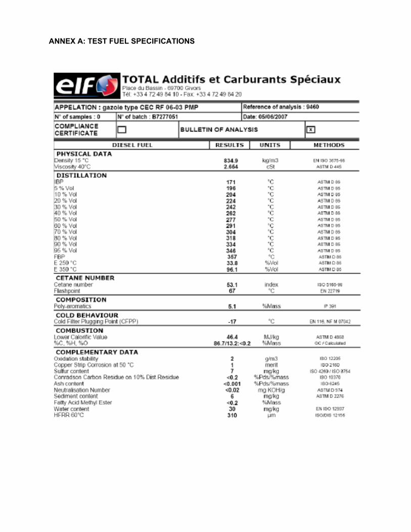
ANNEX A: TEST FUEL SPECIFICATIONS

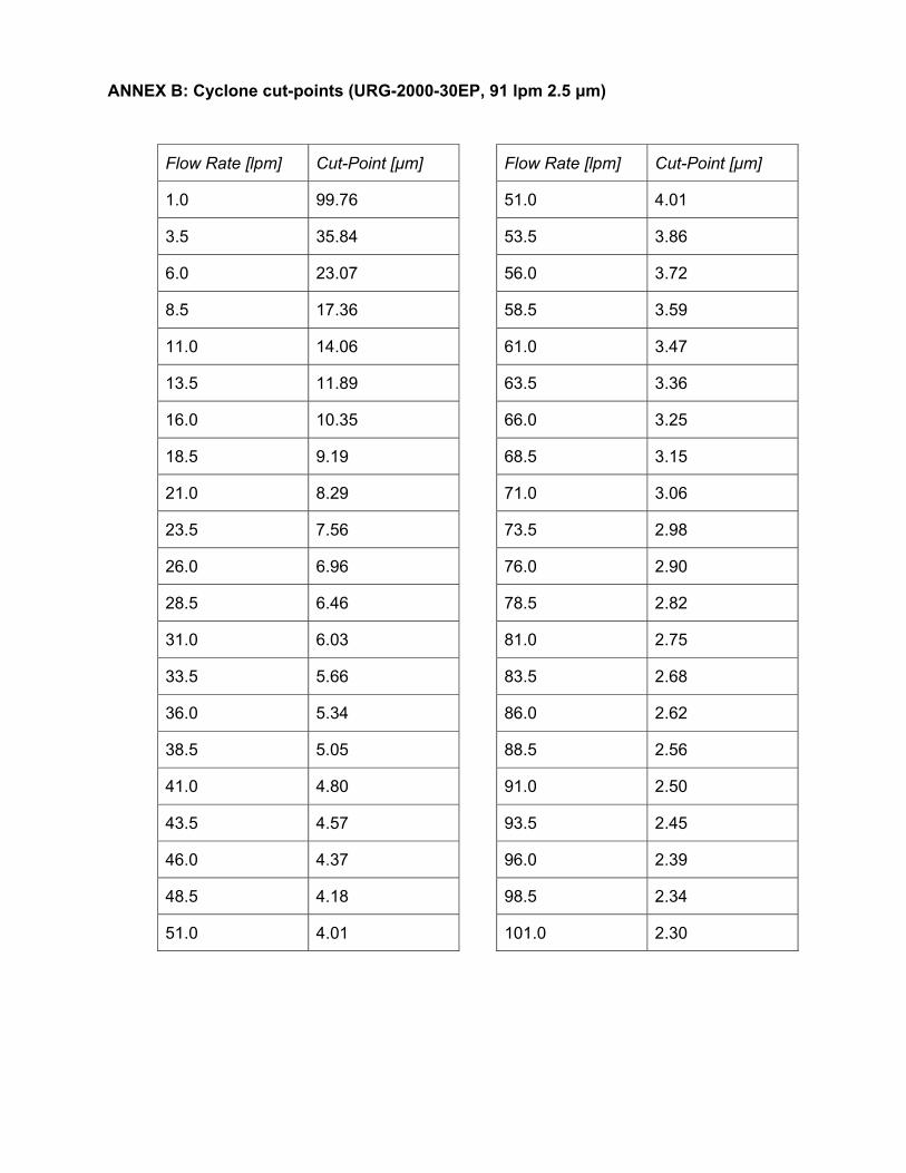
ANNEX B: Cyclone cut-points (URG-2000-30EP, 91 lpm 2.5 μm)

Flow Rate [lpm] Cut-Point [μm] Flow Rate [lpm] Cut-Point [μm]

1.0 99.76 51.0 4.01

3.5 35.84 53.5 3.86

6.0 23.07 56.0 3.72

8.5 17.36 58.5 3.59

11.0 14.06 61.0 3.47

13.5 11.89 63.5 3.36

16.0 10.35 66.0 3.25

18.5 9.19 68.5 3.15

21.0 8.29 71.0 3.06

23.5 7.56 73.5 2.98

26.0 6.96 76.0 2.90

28.5 6.46 78.5 2.82

31.0 6.03 81.0 2.75

33.5 5.66 83.5 2.68

36.0 5.34 86.0 2.62

38.5 5.05 88.5 2.56

41.0 4.80 91.0 2.50

43.5 4.57 93.5 2.45

46.0 4.37 96.0 2.39

48.5 4.18 98.5 2.34

51.0 4.01 101.0 2.30

European Commission EUR 24883 EN – Joint Research Centre – Institute for Energy Title: EU-PEMS PM EVALUATION PROGRAM - Third Report – Further Study on Post DPF PM/PN Emissions Author(s): A. Mamakos, M. Carriero, P. Bonnel, H. Demircioglu, K. Douglas, S. Alessandrini, F. Forni, F. Montigny, D. Lesueur Luxembourg: Publications Office of the European Union 2011 – 87 pp. – 21 x 29.7 cm EUR – Scientific and Technical Research series – ISSN 1018-5593 (print), ISSN 1831-9424 (online) ISBN 978-92-79-20695-5 (print) ISBN 978-92-79-20696-2 (online) doi:10.2788/34166 (print) Abstract This study evaluated the performance of five in total candidate PEMS-PM systems at diesel exhaust PM levels spanning from 20 mg/kWh (Euro V) to post DPF. The different emission levels were simulated by means of a DPF/bypass configuration. The PEMS-PM systems evaluated included Horiba’s On Board System with Transient PM measurement (OBS-TRPM), AVL’s Micro Soot Sensor (MSS) and Gravimetric Filter Box (GFB), Control Sistem’s micro Particulate Sampling System (m-PSS), Sensors Portable Particulate Measurement Device (PPMD) and Dekati’s Mass Monitor (DMM). The work focused on the effect of sampling time on the performance of the PEMS-PM instrumentation. To this end, repeated WHTC tests were performed with PM samples taken over a single WHTC but also over three consecutive test cycles. Teflon filters exhibited superior performance from TX40 and Quartz filters, showing little dependence on the sampling time and at the same time resulting in better agreement between the reference instrumentation and the candidate PEMS-PM systems. The study also evaluated the performance of the real time sensors following some revisions and modifications considered by the manufacturers in response to the findings of the previous (phase 2) campaign. The experimental results verified the improved performance of the revised instrumentation but also revealed some areas for further improvements.

How to obtain EU publications Our priced publications are available from EU Bookshop (http://bookshop.europa.eu), where you can place an order with the sales agent of your choice. The Publications Office has a worldwide network of sales agents. You can obtain their contact details by sending a fax to (352) 29 29-42758.

The mission of the JRC is to provide customer-driven scientific and technical support for the conception, development, implementation and monitoring of EU policies. As a service of the European Commission, the JRC functions as a reference centre of science and technology for the Union. Close to the policy-making process, it serves the common interest of the Member States, while being independent of special interests, whether private or national.

LB-N

A-24883-E

N-C

Documents

EU-PEMS PM EVALUATION PROGRAM - Third Report – Further ...publications.jrc.ec.europa.eu/repository/bitstream/JRC65948/lb-na-24883-en-c.pdf · EU-PEMS PM EVALUATION PROGRAM - Third