1

Optics  simulations  with  Python:  Diffraction    

Ahmed  Ammar*a,  Ritambhar  Burmanb,  Hassen  Ghalilaa,  Zohra  BenLakhdhara,  L.Srinivasa  Varadharajanc  ,  Souad  Lahmara  and  Vasudevan  Lakshminarayanand  

aLSAMA laboratory, Faculty of Sciences of Tunis, University Tunis ElManar, Tunis, Tunisia; bDepartment  of  Electronics  and  Telecommunication  Engineering,  Jadavpur  University,  Kolkata,  India;  cHyderabad  Eye  Research  Foundation,  L  V  Prasad  Eye  Institute,  Banjara  Hills,  Hyderabad  -­‐  500  038,  India;  dUniversity  of  Waterloo  and  University  of  Michigan

 Contact  :  Hassen  Ghalila:  email  :  ghalila.sevestre@planet.tn  

   

Abstract  Python  is  an  easy  open  source  software  that  can  be  used  to  simulate  various  optical  phenomena.  We  have  developed  a  suite  of  programs,  covering  both  geometrical  and  physical  optics.  These  simulations  follow  the  experimental  modules  used  in  the  ALOP  (Active  Learning  in  Optics  and  Photonics)  UNESCO  program  in  the  sense  that  they  complement   it  and   help   with   student   prediction   of   results.   We   present   these   programs   and   the   student   reactions   to   these  simulations.  

Keywords  :  Optics,  Numerical  Experiments,  Python,  Active  Learning,  ALOP,  simulations,  Diffraction,  Physical  Optics.  

   

1.  Introduction    

The  UNESCO  program  “Active  Learning  in  Optics  and  Photonics”  (ALOP)  promotes  a  friendly  and  interactive  method  for   teaching  optics  using   simple   and   inexpensive   equipment   [1-­‐3].  The   full  ALOP  manual   can  be  downloaded   from  UNESCO  [4].  Despite  the  gain  provided  by  these  new  conceptual  experiments,  diffraction  remains  a  difficult  concept  for  students.  Numerical  simulation  is  a  valuable  help  in  this  direction  and  many  simulations  are  now  available  for  free  on  the  web.  Numerical  tools  have  been  developed  to  accompany  the  ALOP  modules  [5,6].  The  dazzling  progress  in  this  area  allow  us,   thanks   to   free  distributions   like  python  and   the  notebook  associated  with   it,   to   implement   the  ALOP  modules  with  the  numerical  code  that  simulate  the  various  phenomena.  .  

 

2.  Teaching  with  python    

Among  the  multitude  of  programming  languages  available,  Python  has  experienced  the  most  rapid  growth  these  past  few  years.  One  reason  for  that  is  due  to  the  fact  that  interfacing  modules  are  multiplatform  so  the  same  program  can  be  used  to  generate  applications  for  different  Operating  Systems  (OS).  Another  important  reason  is  python  is  a  free  and   open   source   software.   In   addition   to   these   two   major   points   python   has   several   advantages   over   other  programming   language   such   as   easy   syntax.   In   addition,   it   comes  with   various   packages   (all   open   source)   such   as  

2

Scipy  (Scientific  Python),  Matplotlib  (a  plotting  program),  Numpy  (Numerical  Python),  Statpy  (Statistical  Python),  etc.  There   are   numerous   texts   on   Python   [7,8].   It   should   be   emphasized   that   Python   is   a   very   intuitive   programming  language,  which  is  very  flexible  and  powerful.  

2.1  Versions  of  Python  One   of   the   most   critical   points   is   the   installation   of   the   python   distribution.   Since   most   of   python   distributions  are/were  developed  as  open  source  a  wide  variety  of  possibilities  are  offered  to  users  and  accordingly  it  is  difficult  to  select   the   one   that   suits   the   user   most.   This   is   particularly   true   when   organizing   an   event   such   as   an   optics  educational   workshop.   In   any   case,   the  most   recommended   version   of   python   to   use   is   python   2.7   because   of   its  stability.  The  newer  version  (Python  3.0  or  3.4)  can  run  version  2.7  with  a  few  minor  modifications.  The  software  can  be  downloaded  from  the  Python  Foundation  at: https://www.python.org/downloads/.    

2.2  Notebook  Notebook  is  a  powerful   tool   to  write  and  generate   lessons   in  various  formats  as   latex,  html  or  slides.   In  addition  to  that   it   is  possible  to   insert  parts  of  codes,  execute  them  and  generate  the  outputs.  This  ability   facilitates  greatly  the  explanation  of  programs.  The  notebook  can  be  downloaded  from:  http://ipython.org/notebook.html.  The  code  given  in  the  section  3.1.3  illustrates  how  to  interactively  affects  a  value  to  one  of  the  parameters.  

3.  Fraunhofer  diffraction  

 

In  this  example  we  will  deal  with  diffraction.  Diffraction  is  one  of  the  modules  of  the  ALOP  program[9].  Fraunhofer  is  an  application  built  using  python  programming  language  and  its  packages  like  Numpy,  Matplotlib  and  wxpython.  This  program  was  developed  under  windows  OS  and  the  same  code  can  be  compiled  under  both  linux  and  OSX.    

3.1  Single  slit  diffraction  

3.1.1  Mathematical  formulation  Single   slit  diffraction   is  modeled  as   sinc()   function  with   the   suitable  parameters.  Let   I(x)  be   the  distribution  of   the  intensity  and  I(0)  its  value  at  x=0.  Let  b  be  the  slit  width,  λ  the  wavelength  and  D  the  distance  of  the  screen  to  the  slit.  The  expression  of  the  intensity  normalized  to  I(0)  is  :  

I(x)I(0)  =  

⎣⎢⎢⎡

⎦⎥⎥⎤sin⎝

⎛⎠⎞πb

λ  xD

⎝⎛

⎠⎞πb

λ  xD

2

  (1)  

Making   these   parameters   interactive,   it   is   possible   to   perform   numerical   experiments   and   test   a   wide   variety   of  configurations.  For  instance,  this  allows  us  to  test  the  effect  of  different  wavelengths,  which  would  be  difficult  to  do  in  an  experimental  situation  due  to  lack  of  light  sources  with  variable  wavelengths.  We  face  the  same  problem  with  the  slits.  For  example,  in  ALOP  workshop  the  slits  are  manually  fabricated.  So  it  is  not  possible  to  produce  a  large  number  of  slits  different  slit  widths.  

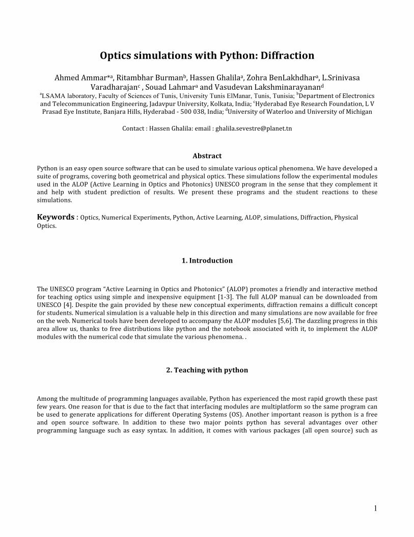
3.1.2  Plotting  within  application  Creating  an  application  with  interactive  tools  as  buttons,  menus,  sliders  make  this  possible.  Figure.1  shows  how  it  is  possible  to  vary  the  three  parameters  (b,  λ,  D)  with  the  help  of  the  sliders  at  the  bottom.  Moreover  the  values  of  these  three   parameters,   displayed   inside   the   plot   along  with   the   formula,   change   simultaneously  with   the   values   in   the  

3

slider.  We  show  here,  as  an  example,  the  interface  created  for  this  application.  

 Figure.1:  Fraunhofer  interface  application  for  a  single  slit  

 

3.1.3  Using  notebook  Notebook  allows  us  to  explain  in  a  friendly  way  how  the  program  is  built.  We  can  follow  the  progress,  as  we  will  do  it  with  a  debugger.  

In  [3]:  %pylab  inline  b=raw_input  ("Enter  the  slit  width  (microns)=  ")  

  print  "b=",b  b  =  b*1.E-­‐06  lamda=  float(600)*1.E-­‐09  D=  float(100)*1.E-­‐02  thetamin1=  -­‐np.pi/200  thetamax1=  np.pi/200  pas  =(  thetamax1-­‐thetamin1)/2001  Theta1=[]  for  i  in  range(2001):            T1  =  thetamin1+i*pas            Theta1.append(T1)            U1  =  np.pi*b*np.sin(Theta1)/lamda            Amplitude=  np.sin(U1)  /  U1            Intens_1f=Amplitude**2            U1  =  1.E+2*np.tan(Theta1)*np.array(D)    We  get  as  an  output  :  Enter  the  slit  width  (microns)=  1  b = 1

4

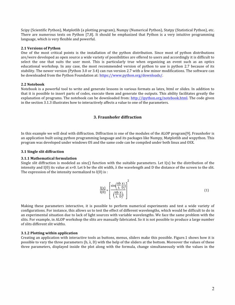
This  first  part  affects  the  value  to  the  three  parameters  (d,  λ,  D)  and  computes  the  sinc()  function.  The  following  part  displays  the  result.  

In  [4]:  fig  =  plt.figure()  ax1=fig.add_subplot(1,1,1)  ax1.plot(U1,  Intens_1f,’r-­‐’)  ax1.set_xlabel(’cm’)  ax1.set_ylabel(’Intensity’)  ax1.grid(True)    

   Figure.2:  Direct  display  of  the  portion  of  code  given  above  

3.2  Multiple  slit  diffraction  

3.2.1  Young’s  Double  slit  diffraction  As  in  the  previous  section,  let  I(x)  be  the  distribution  of  the  intensity  and  I(0)  its  value  at  x=0.  Let  ‘b’  be  the  slit  width,  ‘a’   the  distance  between  slits,   ‘λ’   the  wavelength  and   ‘D’   the  distance  of   the  screen  to  the  slit.  The  expression  of   the  intensity  normalized  to  I(0)  is  :  

I(x)I(0)  =  4  

⎣⎢⎡

⎦⎥⎤sin⎝

⎛⎠⎞πb

λ  xD

⎝⎛

⎠⎞πb

λ  xD

2

 ⎣⎡

⎦⎤cos⎝

⎛⎠⎞πa

λ  xD  

2   (2)  

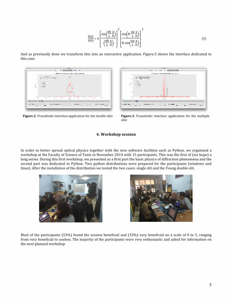
We  proceed  with  the  same  way  as  in  the  case  of  the  single  slit.  Making  these  parameters  interactive,  it  is  possible  to  perform  numerical  experiments  and  test  a  wide  variety  of  configurations.  Figure.2  shows  how  it   is  possible  to  vary  the   four  parameters  (b,  a,  λ,  D)  with   the  help  of   the  sliders  at   the  bottom.  Likewise   these   four  values  are  displayed  inside  the  plot  along  with  the  formula  changing  simultaneously  with  the  values  in  the  slider.

3.2.2  Diffraction  grating    Increasing  the  number  of  slits  lead  us  to  the  case  of  grating  diffraction.  In  this  case  the  mathematical  expression  of  the  normalized  intensity  is  given  by:  

5

I(x)I(0)  =  4  

⎣⎢⎢⎡

⎦⎥⎥⎤sin⎝

⎛⎠⎞πb

λ  xD

⎝⎛

⎠⎞πb

λ  xD

2

 

⎣⎢⎢⎡

⎦⎥⎥⎤sin⎝

⎛⎠⎞N  

πaλ  xD

N  sin⎝⎛

⎠⎞πa

λ  xD

 

2

  (3)  

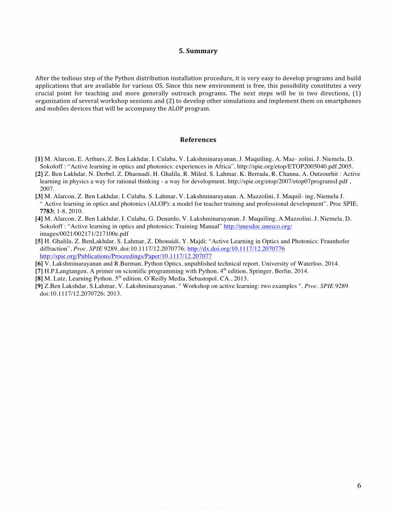
And  as  previously  done  we  transform  this   into  an   interactive  application.  Figure.3  shows  the   interface  dedicated  to  this  case.  

   Figure.2:  Fraunhofer  interface  application  for  the  double  slits   Figure.3:   Fraunhofer   interface   application   for   the  multiple  

slits  

4.  Workshop  session    

In   order   to  better   spread  optical   physics   together  with   the  new   software   facilities   such   as  Python,  we  organized   a  workshop  at  the  Faculty  of  Science  of  Tunis  in  November  2014  with  15  participants.  This  was  the  first  of  (we  hope)  a  long  series.  During  this  first  workshop,  we  presented  as  a  first  part  the  basic  physics  of  diffraction  phenomena  and  the  second  part  was  dedicated   to  Python.   Two  python  distributions  were  prepared   for   the  participants   (windows   and  linux).  After  the  installation  of  the  distribution  we  tested  the  two  cases:  single  slit  and  the  Young  double  slit.  

     

Most  of   the  participants   (53%)   found   the  session  beneficial  and  (33%)  very  beneficial  on  a  scale  of  0   to  5,   ranging  from  very  beneficial  to  useless.  The  majority  of  the  participants  were  very  enthusiastic  and  asked  for  information  on  the  next  planned  workshop  

6

5.  Summary    

After  the  tedious  step  of  the  Python  distribution  installation  procedure,  it  is  very  easy  to  develop  programs  and  build  applications  that  are  available   for  various  OS.  Since  this  new  environment   is   free,   this  possibility  constitutes  a  very  crucial   point   for   teaching   and   more   generally   outreach   programs.   The   next   steps   will   be   in   two   directions,   (1)  organization  of  several  workshop  sessions  and  (2)  to  develop  other  simulations  and  implement  them  on  smartphones  and  mobiles  devices  that  will  be  accompany  the  ALOP  program.  

 

References   [1] M. Alarcon, E. Arthurs, Z. Ben Lakhdar, I. Culaba, V. Lakshminarayanan, J. Maquiling, A. Maz- zolini, J. Niemela, D.

Sokoloff : “Active learning in optics and photonics: experiences in Africa”, http://spie.org/etop/ETOP2005040.pdf,2005. [2] Z. Ben Lakhdar, N. Derbel, Z. Dhaouadi, H. Ghalila, R. Miled, S. Lahmar, K. Berrada, R. Channa, A. Outzourhit : Active

learning in physics a way for rational thinking - a way for development. http://spie.org/etop/2007/etop07programsI.pdf , 2007.

[3] M. Alarcon, Z. Ben Lakhdar, I. Culaba, S. Lahmar, V. Lakshminarayanan, A. Mazzolini, J. Maquil- ing, Niemela J. “ Active learning in optics and photonics (ALOP): a model for teacher training and professional development”, Proc SPIE, 7783: 1-8, 2010.

[4] M. Alarcon, Z. Ben Lakhdar, I. Culaba, G. Denardo, V. Lakshminarayanan, J. Maquiling, A.Mazzolini, J. Niemela, D. Sokoloff : “Active learning in optics and photonics: Training Manual” http://unesdoc.unesco.org/ images/0021/002171/217100e.pdf

[5] H. Ghalila, Z. BenLakhdar, S. Lahmar, Z. Dhouaidi, Y. Majdi: “Active Learning in Optics and Photonics: Fraunhofer diffraction”, Proc. SPIE 9289, doi:10.1117/12.2070776; http://dx.doi.org/10.1117/12.2070776 http://spie.org/Publications/Proceedings/Paper/10.1117/12.207077

[6] V. Lakshminarayanan and R.Burman, Python Optics, unpublished technical report, University of Waterloo, 2014. [7] H.P.Langtangen, A primer on scientific programming with Python, 4th edition, Springer, Berlin, 2014. [8] M. Lutz, Learning Python, 5th edition, O’Reilly Media, Sebastopol, CA., 2013. [9] Z.Ben Lakshdar, S.Lahmar, V. Lakshminarayanan, " Workshop on active learning: two examples ", Proc. SPIE 9289

doi:10.1117/12.2070726; 2013.