Embed Size (px)
Citation preview

C E N T R ED ’ É T U D E S P R O S P E C T I V E SE T D ’ I N F O R M A T I O N SI N T E R N A T I O N A L E S
No 2011 – 24December
DO
CU
ME
NT
DE
TR
AV
AI
L
Estimations of Tariff Equivalentsfor the Services Sectors
Lionel Fontagné Amélie Guillin Cristina Mitaritonna
We acknowledge financial support from the CIREM.
TABLE OF CONTENTS
Non-technical summary . . . . . . . . . . . . . . . . . . . . . . . . . . . 3Abstract . . . . . . . . . . . . . . . . . . . . . . . . . . . . . . . . . 5Résumé non technique . . . . . . . . . . . . . . . . . . . . . . . . . . . 6Résumé court . . . . . . . . . . . . . . . . . . . . . . . . . . . . . . . 71. Introduction . . . . . . . . . . . . . . . . . . . . . . . . . . . . . . 82. Quantifying trade barriers in services . . . . . . . . . . . . . . . . . . . . 103. Data . . . . . . . . . . . . . . . . . . . . . . . . . . . . . . . . . 134. Methodology . . . . . . . . . . . . . . . . . . . . . . . . . . . . . 14
4.1. Gravity equations estimated on cross-sectional reconstructed data . . . . . . . 144.2. Gravity equations estimated using actual panel data. . . . . . . . . . . . . 164.3. Derivation of tariff equivalents . . . . . . . . . . . . . . . . . . . . . 17
5. Estimation results . . . . . . . . . . . . . . . . . . . . . . . . . . . . 195.1. Beyond Park’s specification: regression results on (cross section) reconstructeddata. . . . . . . . . . . . . . . . . . . . . . . . . . . . . . . . . . 195.2. Considering the zero flows . . . . . . . . . . . . . . . . . . . . . . 215.3. Regression results from estimations on actual data . . . . . . . . . . . . . 23
6. Tariff equivalents . . . . . . . . . . . . . . . . . . . . . . . . . . . . 247. Conclusion . . . . . . . . . . . . . . . . . . . . . . . . . . . . . . 30
References . . . . . . . . . . . . . . . . . . . . . . . . . . . . . . 318. Appendix . . . . . . . . . . . . . . . . . . . . . . . . . . . . . . . 33
8.1. Cross section estimations using GTAP data . . . . . . . . . . . . . . . . 338.2. Ad-valorem equivalents by country from cross section estimations using GTAPdata. . . . . . . . . . . . . . . . . . . . . . . . . . . . . . . . . . 388.3. Reliability . . . . . . . . . . . . . . . . . . . . . . . . . . . . . 408.4. RTAs . . . . . . . . . . . . . . . . . . . . . . . . . . . . . . . 42
List of working papers released by CEPII . . . . . . . . . . . . . . . . . . . . 43
2
ESTIMATIONS OF TARIFF EQUIVALENTSFOR THE SERVICES SECTORS
NON-TECHNICAL SUMMARY
Services is the largest sector in the global economy, representing 70% of world added value and overhalf of total employment. However its share in total international trade is only 21%, in part due to thehigh level of regulatory protection in domestic markets for services. Simulations relying on ComputableGeneral Equilibrium (CGE) modeling point to large gains associated with the partial liberalization ofservices in the rich economies, but also in some developing countries. Since these estimations rely ontariff equivalents of protection on services, accurate measure of the level of protection on services are acrucial issue for policy makers.
One problem lies in the specific nature of services compared to goods. Proximity between producer andconsumer and the intangible characteristics intrinsic to services produce different impediments to tradein services from those that apply to goods. They include limitations such as quotas, licences, interdic-tions of some activities to foreigners, and government regulations designed to reduce market access toforeign services and/or discriminate in favor of domestic firms. Hence, liberalizing national trade inservices essentially requires a change in national regulation. Identifying the actual tariff equivalents ofthese regulations is not straightforward. Data on actual policies are scarce and transforming qualitativeinformation into a quantitative measure of protection is difficult. Therefore, we depart from the inven-tory approach used to build indexes of the restrictiveness of policies in the service sector, and also fromthe so-called two-stage method, in which information on barriers faced by exporters of services on theirdestination markets is used to explain international differences in price-cost margins within the servicessectors.
The context is appropriate for an indirect approach consisting of computing tariff equivalents and re-vealing protection by comparing actual trade in services against a benchmark. The distribution of theresiduals of a gravity equation estimated at the sectoral level can be used for this computation; alterna-tively, we can compute the average protection applied by each importer, from the importer fixed effectscoefficients. We employ this latter procedure, which is an improvement on the methodology of Park(2002). We compute regulation tariff equivalents focusing on cross border trade in services (Mode 1)and provide evidence on the magnitude of the different estimation biases potentially associated with thismethod.
We provide tariffs equivalents for 9 services sectors and 65 countries based on Global Trade AnalysisProject (GTAP) data. The countries with the lowest levels of protection are the developed economies.The most liberalized sector is Transport with a 26% tariff protection on average. The most protected isConstruction, with an average tariff of 75%.
Our tariff equivalents are computed using a fixed effects methodology which is shown to be preferable tothe traditional approach based on normalized residuals of the gravity equation. This means that, with theexception of Transport and Business Services for which figures are comparable, our tariffs are higher.
The results based on actual panel data are quite different from the results obtained for the cross sectionGTAP data. Those differences are due to the data (reconstructed versus actual) not the methodology(cross section versus panel). It should be noted, therefore, that using partially ’‘reconstructed data’ to
3

estimate tariff equivalents may bias results. However, the hierarchy of countries within sectors in termsof the protection obtained using the reconstructed data set is fairly reliable, and most divergences arerelated to developing economies. Therefore we can be fairly confident about the accuracy of the tariffequivalents of protection in services trade proposed here.
4
ABSTRACT
Methodological issues arising from the estimation of tariff equivalents of barriers to services trade arevery relevant for policy. These equivalents are used extensively to compute welfare gains and resourcereallocations associated with partial liberalization of the sector; any measurement errors will stronglyaffect the estimated gains. Using the Global Trade Analysis Project (GTAP) database, we rely on so-called quantity based methods to derive tariff equivalents from a gravity equation estimated at sectorallevel for 9 services sectors and 65 countries.
We also estimate trade equations for services using cross section data, and improve on the methodologyof Park (2002). We investigate whether relying on cross section rather than panel data leads to dif-ferences in the estimated equivalents. Finally, we compare the estimations based on reconstructed andactual data. We conclude that although use of partially reconstructed data (such as GTAP) affects theresults, the equivalents obtained are good representations of the magnitude of protection for services inthe various countries analyzed, although with larger deviations for developing economies.
JEL Classification: F13.
Keywords: Market access, tariffs, trade in services
5
LE CALCUL D’ÉQUIVALENTS DROITS DE DOUANE DANS LE COMMERCE DE SERVICES
RÉSUME NON TECHNIQUE
Les services représentent le secteur le plus important de l’économie, avec 70% de la valeur ajoutée mon-diale et plus de la moitié de l’emploi total. Toutefois, leur part dans les échanges mondiaux reste limitée(21% du commerce mondial en valeur), en partie en raison des niveaux élevés de protection réglemen-taire des marchés nationaux. Les simulations réalisées avec des Modèles d’Equilibre Général Calculableconcluent à des gains importants à la libéralisation des échanges de services pour les économies avancéescomme pour les pays en développement. Comme ces estimations sont fondées sur l’utilisation d’équi-valents droits de douane de la protection réglementaire des activités de services, la mesure correcte deces équivalents est une question importante pour la politique économique.
Une première difficulté tient à la nature spécifique des services, comparés aux biens. La proximité entreproducteur et consommateur est souvent nécessaire ; en raison de leur nature intangible les obstacles auxéchanges de services diffèrent de ceux auxquels sont confrontés les échanges de biens. Ces obstaclesprennent la forme de quotas, de licences, d’interdiction d’exercer certaines activités pour les étrangers,ou encore d’accès privilégié pour les entreprises nationales. Ainsi, libéraliser les échanges de servicessignifie-t-il pour un pays une adaptation de ses réglementations. Mais la valeur exacte de l’équivalentdroit de douane des réglementations existantes est une question complexe. D’autant que les données surles réglementations appliquées sont rares et que transformer cette information qualitative en indicateurquantitatif est difficile. Nous nous écartons donc de l’approche dite de l’inventaire utilisée dans la litté-rature pour construire des indices de restrictivité. Nous nous écartons aussi de l’approche en deux étapesconsistant à utiliser l’information sur les barrières auxquels font face les opérateurs étrangers, pour ex-pliquer les taux de marge des firmes dans les pays utilisateurs.
Une approche indirecte est en effet envisageable. Il s’agit de révéler la protection en comparant le com-merce de services observés à une norme. On calcule alors le droit de douane équivalents à la protectionréglementaire. La distribution des résidus de l’équation de gravité estimée au niveau sectoriel peut êtreutilisée à cette fin. Une méthode alternative consiste à calculer la protection appliquée par chaque impor-tateur en exploitant les effets fixes importateurs dans une telle équation. Nous adoptons ici cette stratégieet utilisons une méthode d’estimation plus satisfaisante que celle de Park (2002). Nous calculons finale-ment les droits de douane équivalents dans le commerce transfrontières de services (Modalité 1). Nousdocumentons les différents biais d’estimation associés à cette approche.
Nous proposons finalement des équivalents droits de douane pour 9 secteurs de services et 65 pays fon-dés sur les données du consortium Global Trade Analysis Project (GTAP). Il apparaît que les économiesavancées sont celles protégeant le moins leur secteurs de services. Les secteurs les plus libéralisés sontle transport avec un équivalent droit de douane moyen de 26% ; à l’opposé la construction est le secteurle plus protégé (respectivement 75%).
Les résultats obtenus sur données de panel réelles diffèrent toutefois de ceux en coupe instantanée ex-ploitant la base du consortium GTAP. Nous montrons que ces différences sont dues aux données (re-
6
construites versus réelles) et non à la méthode (coupe versus panel). Ceci souligne que l’utilisation dedonnées partiellement reconstruites pour calculer des équivalents droits de douane peut biaiser les ré-sultats. Toutefois, la hiérarchie des pays au sein des secteurs, en termes de protection, est malgré toutassez fiable et l’essentiel des divergences concerne des pays en développement. Nous pouvons donc êtrerelativement confiants dans la validité des équivalents droits de douane de la protection des servicesproposés ici.
RÉSUMÉ COURT
Le calcul d’équivalents droits de douane des obstacles aux échanges de services représente un enjeuimportant pour la politique économique. Ces équivalents sont largement utilisés pour calculer les gainsde bien être et les réallocations de ressources consécutifs à la libéralisation partielle des échanges dansce secteur. Aussi toute erreur de mesure est-elle de nature à affecter significativement les gains estimés.Nous utilisons la base de données d’échanges de services du Global Trade Analysis Project (GTAP) etnous appuyons sur la méthode dite des quantités, fondée sur une équation de gravité, pour calculer deséquivalents droits de douane dans 9 secteurs de services et 65 pays.
Outre le calcul de ces équivalents, nous estimons des équations de commerce international de servicesen coupe et améliorions la méthodologie de Park (2002). Nous examinons éalement si l’utilisation dedonnées de panel fait une différence importante. Enfin nous confrontrons les résultats d’estimationss’appuyant sur des données partiellement reconstruites (comme celles de GTAP) et sur des donnéesréelles. Nous montrons que si l’utilisation de données partiellement reconstruites affecte les résultats,les équivalents droits de douane ainsi obtenus caractérisent correctement l’ampleur de la protection dansles services dans les différents pays, avec toutefois des écarts plus importants dans le cas des pays endéveloppement.
Classification JEL : F13.
Mots clés : Protection dans les Services, équivalent droits de douane, commerce de services.
7
ESTIMATIONS OF TARIFF EQUIVALENTSFOR THE SERVICES SECTORS
Lionel Fontagné ∗
Amélie Guillin †
Cristina Mitaritonna ‡
1. INTRODUCTION
Services is the largest sector in the global economy, representing 70% of world added value andover half of total employment. However, the share of services in total trade is lagging despitehaving expanded greatly since the 1980s. Services account for 21% of total international trade(World-Trade-Organization, 2010), and thanks to major technological progress its importanceis expected to increase in the future.
There has been a greater willingness in recent years to include services in bilateral as well asmultilateral trade agreements. In the multilateral arena, services were not initially included innegotiations. Their inclusion in the Uruguay Round, led to the General Agreement on Tradein Services (GATS) in January 1995. The GATS relates to the multilateral liberalization of150 different services sectors, distinguishing between four modes of supply, whose relativeimportance differs among sectors: 1
• Mode 1 or Cross-border supply (e.g. financial operation).• Mode 2 or Consumption abroad (tourism).• Mode 3 or Commercial presence (Foreign Direct Investment – FDI).• Mode 4 or Presence of natural persons (temporary workers migrations).
As a result of the growing role of services in world trade, economists have started to pay moreattention to this field (Francois et al., 2009). Simulations based on Computable General Equi-librium (CGE) modeling point to the large gains associated with the partial liberalization ofservices. Sizable gains can be expected for the rich economies, but also for developing coun-tries, especially India and China (Francois et al., 2005; Decreux and Fontagné, 2011).
Since these estimates rely on tariff equivalents of protection for services, an accurate measureof the level of protection in services is key to the assessment of the gains from liberalization.However, computing tariff equivalents can be challenging, both theoretically and empirically.
∗. Paris School of Economics (University of Paris I) and CEPII. [email protected].†. Paris School of Economics (University of Paris I). [email protected]‡. CEPII. [email protected]. The 150 sectors are aggregated into macro-categories: business services, communication, construction and
engineering, distribution, education, finance, environmental services, tourism, health and other social services,transport and recreational services.
8
A first problem is related to the specific nature of services compared to goods. Proximity be-tween producer and consumer and the intangible characteristics intrinsic to services producedifferent impediments to trade in services from those that apply to goods. These impedimentsinclude limitations such as quotas, licences, prohibition of some activities for foreigners, andgovernment regulations intended to reduce market access for foreign firms and/or discriminatein favor of domestic firms. Liberalizing trade in services implies changes to national regulation.From a technical and a political economy perspective, reformulating regulations implies muchmore than simply cutting a tariff.
A second problem is the scarcity of data on actual policies, and the methodological issuesraised by the use of qualitative data. Collecting information on domestic regulation, its de-gree of restrictiveness and its coverage for each sector and importer, is an immense task. Ifthis information is made available through surveys, indices have to be constructed and used asregressors of price cost margins (Dee, 2005; Dihel and Shepherd, 2007; Fontagné and Mitari-tonna, 2009). The OECD has embarked on the construction of Services Trade RestrictivenessIndices (STRI), which are a quantitative measure derived from qualitative information. TheWorld Bank has produced the Global Services Policy Restrictiveness Database which is basedon the results of a survey of 102 countries and 5 sectors: financial services, telecommunica-tions, retail distribution, transportation and business services (Borchert et al., 2011). Even if theinformation is available, its treatment is problematic. Survey results have to be summarized inan index that maps regulations on an arbitrary scale of restrictiveness. When available, resultsfor the different modes need to be aggregated using rather arbitrary weights.
This suggest an indirect approach (Park, 2002; Francois et al., 2005; Walsh, 2006), consistingof computing tariff equivalents and assessing protection by comparing actual trade in servicesagainst a benchmark. The distribution of the residuals of a gravity equation estimated at sectorallevel can be used for this computation. Alternatively, we can compute the average protectionapplied by each importer from importer fixed effects coefficients. The data can be cross sectionor panel data. Because of the scarcity of information, the source can be either reconstructeddata if the sample is comprehensive, or actual data, but for only a limited number of countries.This approach cumulates the issues related to reliance on gravity estimates, with problems spe-cific to the source data. Our objective is to address these problems systematically and computead valorem equivalents (AVEs) for trade in services relying on this indirect approach.
This paper makes two contributions. First, it highlights the potential problems related to es-timating tariff equivalents for trade in services from a gravity equation: we provide evidenceof the magnitude of the related estimation bias. Second, it provides tariff equivalents for 9services sectors and 65 countries, which can be used to estimate the welfare effects of liberal-ization of services trade. Overall, our tariff equivalents are much higher than for goods. Foran industrialized country, tariffs typically range between 0% and 50%-60% depending on thesector. In the construction sector the barriers may be even higher than this and in several devel-oping countries and for certain sectors, tariff equivalents may be above 100%. These measuresare sensitive to the elasticity of substitution chosen and accordingly should be considered withsome caution. However, the elasticity of substitution has no impact on the hierarchy of coun-
9
tries within sectors.
The rest of the paper is organized in five sections. Section 2 presents the theoretical and empir-ical issues related to the gravity approach and briefly reviews the literature on gravity modelsapplied to services. The data are described in Section 3 and Section 4 discusses the empiricalapproach. Section 5 presents the results and Section 6 concludes.
2. QUANTIFYING TRADE BARRIERS IN SERVICES
Several attempts have been made to quantify barriers to services trade. There is a strand ofliterature that is based on inventory approaches. In a seminal paper Hoekman (1996) usesa methodology based on a frequency index, which assigns a numerical value to the level ofrestrictions imposed by each country in a given sector, by mode of supply. 2 The country’sGATS commitment schedule is used as the main source of information on the barriers imposedby countries. An arbitrary tariff equivalent is then attributed to the country demonstrating themost protectionist policy. Other countries’ tariff equivalent are calculated according to the levelof their commitment relative to the benchmark. Stern (2000) points out that the Hoekman in-dices are relative indicators not real indices that can be used as tariff equivalents. Mattoo et al.(2001) build openness indices for telecommunications and financial services to analyze the ef-fects on growth of services liberalization. The first index is based on the market structure ofthe sector (competitive or not), on FDI (allowed or not) and on the presence (or not) of an in-dependent regulator. The other index (the so-called ’financial index’) combines information onmarket structure, capital controls (the Dailami index) and the level of foreign equity. Financialindices ordering shows that liberalized countries are generally the most developed countries.However, for telecommunications the indices show that some developing countries such as ElSalvador and Ghana, are quite open. Concerns regarding data reliability and availability usingthis method as well as Hoekman’s are summarized in Chen and Schembri (2002). Gootiiz andMattoo (2009) compile actual policy restrictiveness in the services sector for 32 developing andtransition economies, and 24 OECD countries. The degree of protection is compared to Dohaoffers and Uruguay round commitments. A synthetic index is calculated by country and sectorfor the three levels of restrictiveness, but no AVE is proposed.
A second strand of literature examines the barriers to trade in services relying on a two-stagemethod. The first stage consists of qualitative assessment of the commitments made by im-porters under the GATS, or of the barriers imposed on exporters of services by destination mar-kets. In the second stage, the same information is used to explain international differences inprice-cost margins within sectors. The Australian Productivity Commission (APC) pioneeredthe estimation of tariff equivalents using the Trade Restrictiveness Indices (TRI) (Dee, 2005). 3
2. A weight of 1 is attributed to a sector or a mode with no restrictions, 0 if no policy binds and 0.5 if there isany restriction in a sector or in a mode of supply.
3. A set of qualitative data on barriers is used to build quantitative indexes which are used in econometricmodels to explain economic performance in order to obtain tariff equivalents: controlling for firm-level variables,price-cost margins are regressed on TRI. Note that these indexes are different from Anderson-type TRI based ondifferent methodologies, despite the similar acronym.
10
Relying on a weighting methodology, Dihel and Shepherd (2007) apply the same methodologyas the APC. They observe that the non-OECD trade restrictiveness indexes are higher than theOECD indexes. The method is extended in Fontagné and Mitaritonna (2009) and applied to theDistribution and Telecoms sectors in emerging countries. Kox and Nordas (2007) examine howdomestic regulation affects trade in services under mode 3 (commercial presence), proxied bythe stock of FDI.
Finally, there is a strand of literature showing that the level of protection in services can be re-vealed through an econometric exercise relying on a gravity equation. Since Tinbergen (1962),the gravity equation has been used extensively in the empirics of international trade, becauseof its remarkably good predictions of bilateral trade flows in goods. Although it was criticizedinitially for its lack of theoretical foundations, the gravity equation can be derived from variousformal trade models under a wide range of modeling assumptions. 4 Essentially a gravity equa-tion is an expenditure equation with a market clearing condition imposed. Two price terms,labeled as multilateral resistance terms following Anderson and van Wincoop (2003), appearinto the equation. These terms are quite complex, and not directly observable because theyinclude missing data, for instance, number of the varieties consumed or producer price of eachvariety. The problem here is that the omitted terms are correlated with the trade cost term be-cause they are a function of the bilateral trade costs. This correlation mean that the estimates ofthe trade cost determinants are biased. The main value added by Anderson and van Wincoop(2003) is derivation of a practical way of using the full expenditure system to estimate key pa-rameters on cross-section data and to show that including country specific fixed effects yieldsthe same results. With panel data, however, the problem is more severe. If we assume that omit-ted terms vary over time, including time-invariant country dummies removes the cross-sectionbias, not the time series dimension. Thus, a good solution is to include time-varying countrydummies. The alternative of a time-varying pair dummy is rarely useful, since most gravitymodels are aimed at identifying bilateral trade barriers which would be impossible to estimatesince they are already captured by pair fixed effects.
In contrast to work demonstrating the effectiveness of the gravity equation applied to tradein goods, the literature on application of the gravity model to services trade, pioneered byFrancois (1993), is limited. However, it has increased since 2000 (Mirza and Nicoletti, 2004;Kimura and Lee, 2006; Francois et al., 2009), due mainly to improved data quality althoughthe availability of information on services trade still lags behind information on trade in goods.Francois et al. (2005) rely on sector-specific gravity equations estimated on data from the GTAPand show that, to estimate trade barriers, the standard specification is significant even for tradein services. Kimura and Lee (2006) confirm that Gross Domestic Product (GDP), distance,remoteness, adjacency, Regional Trade Agreement (RTA), economic freedom index and com-
4. For examples of the theoretical foundation of the gravity equation see, e.g., Anderson (1979), Helpmanand Krugman (1985), Bergstrand (1990), Deardorff (1998), Feenstra (2002), Feenstra (2004), Anderson and vanWincoop (2003), Helpman et al. (2007), Melitz and Ottaviano (2008). The development of the theoretical modelshas been useful for explaining why, despite the goodness of fits, results from estimations of bilateral trade costsvariables may be severely biased. Baldwin and Taglioni (2006) provide for a minimalist derivation of the gravityequation furnishing estimates of the size of the biases commonly found in the literature, taking currency union asan example.
11
mon language are significant and robust determinants of bilateral trade in services (importsand exports). Walsh (2006) estimates a specific gravity equation for four sectors (transport,government, other commercial services, and travel). The explanatory variables are per capitaGDP, population, distance, adjacency, common language and a dummy for European Unionmembership. All the variables are statistically significant and have the expected impact on thevalue of bilateral trade. However, interpretation of the results for distance should be cautious. 5
For the computation of tariff equivalents based on the gravity equation, the approach proposedby Park (2002) and using the residuals of this equation is generally supported by applied modelsaddressing the economic impact of liberalization of trade in services. The gravity equation usedis based on Deardorff (1998) and considers the most commonly used explanatory variablesin gravity equation used such as GDP, distance and language. We elaborate on Park’s worklater in the paper. Note, however, that Park (2002) departs from Anderson and van Wincoop(2003) regarding how prices are tackled. Park’s results for the estimation of tariff barriersfor seven different sectors are very different from Hoekman (1996). From an elasticity ofsubstitution of 4.67, the tariff equivalents computed by Francois et al. (2005) are based onthe actual to predicted trade ratio. With this method, India is the least opened country whileSub-Saharan Africa and Netherlands have 0% trade cost equivalents for the four categories ofservices considered. Using a similar method to Park’s, but with an elasticity of substitutionof 1.95, Walsh (2006) finds average tariff equivalents ranging from 0% (Japan, Norway andBelgium) to 125% (Indonesia). Francois et al. (2009) rely on a large sample of importingcountries (39 or 49 depending on the sector) and estimate the elasticity of trade in services tothe presence of Non Tariff Barriers (NTBs) using a probit selection estimator (up to 40% oftheir bilateral observations are zeros for business and information and computer and telecomservices). They apply this estimation to 6 service sectors, using data for 2004-2006. Theyinteract the OECD’s openness index for operations of multinational enterprises (FDI restrictionindex) with dummies for regional trade agreements. The computed trade elasticities range from-0.5 (communications) to -8.7 (personal and cultural recreation). For business and Informationand Communication Technologies (ICT), Insurance, Finance and Construction, the range is -2.0 to -4.2. If we assume that trade costs vary in proportion to the OECD openness index, whatis obtained can be considered to be import price elasticities.
It can be seen that potentially there are numerous methodological issues that can arise in usingthe gravity method. First, the distribution of the residuals of the estimated equation is sensitiveto specification and omitted variables problems which affect the estimation of tariff equivalents.Hence, it might be preferable to rely on a strategy based on country fixed effects. Second, it isnecessary to make an assumption about the elasticity of substitution to transform the parameterestimate into an AVE. The value of the equivalents is highly sensitive to this assumption. Third,since sectoral and bilateral data on trade in services is scarce, many papers rely on reconstructeddata, based on econometrics, which a priori is questionable.
In order to highlight the various problems associated with the gravity method, in this paper weestimate tariff equivalents for the service sectors, focusing on cross border trade in services(Mode 1). We rely on so-called quantity based methods. Initially we estimate services trade
5. In the case of services, compared to goods, distance has a different meaning, which is due to the intangiblenature of what is being traded. This variable may be capturing informational imperfections in particular.
12
equations on cross section data. We use the most recent version of the GTAP database providedby the Netherlands Bureau of Economic Analysis (CPB thereafter) for 2004. Using the samesource data as Park (2002), but for a more recent cross section, we prefer a methodology basedon country fixed effects. We provide estimates of trade barriers for a larger set of countries(65 vs 51) and sectors. The robustness of these estimations is systematically challenged byaddressing the methodological issues referred to above.
3. DATA
We draw on a relative small set of data sources. The main source of data used in the first stageof this paper is the GTAP database which provides bilateral trade in services for 14 servicessectors for the year 2004: Construction (cns), Communication (cmn), Trade (trd), Finance (ofi),Other services (osg) comprising education, health, defense and public administration, Business(obs), Air transport (atp), Water transport (wtp), Other transport (otp), Insurance (irs), Recre-ational services (ros) and Dwellings (dwe), Water (wtr) and Energy (ely). 6 In line with Park(2002) we consider the same seven services sectors originally studied: cmn, cns, obs, trn, trd,ofi, osg. Trn, which is Transport, includes the three transport sectors (atp, wtp and otp). How-ever, in the alternative estimation strategy we add two more sectors: isr and wtp.
The number of countries varies according to the different versions of the GTAP database. The7.4 release includes 82 regions, but fewer individual countries, 7 which allows a large represen-tation of both developed and developing countries. Unfortunately not all are single countries,some are regions made up of Least Developed Countries and Developing Countries. 8 We de-cided these amalgamations, as both importers and exporters, due to the problem of using controlvariables for non-single countries. When deleting a region as an exporter we were careful toretain single countries as importers if we had 70% of their bilateral trade in the remaining data.
There are IMF data on GDP and on Producer Price Indexes (or Wholesale Price Indexes forsome countries) for the year 2004. Population data are from the World Bank (World Devel-opment Indicators – WDI). Distances and all remaining control variables are from the CEPIIdatabase. 9 For some countries, namely Bostwana, Malawi, Morocco, Mozambique, Tanzania,Uganda, Zambia and Zimbabwe, we do not have data on Producer Price Indexes and, therefore,cannot estimate tariff equivalents for them when prices are used as regressors in the gravityestimation.
The reliability of the data is fundamental for our analysis; van Leeuwen and Lejour (2008) ad-dress the quality of GTAP and OECD data. They compute reliability indices for 1999-2003 and
6. We rely on release 7.4 of the database. See https://www.gtap.agecon.purdue.edu/7. Park relies on version 5, which includes 52 countries, for his estimation for 1997. The presence in Park’s
work of tariff equivalents for Botswana, Uganda, Mozambique, Tanzania, Malawi and the Zambia is puzzling,since the producer price indexes for these countries are not available in IMF data for 1997.
8. This applies particularly to African countries. Israel is not documented individually in GTAP.9. The database is freely available on the CEPII Web site http://www.cepii.fr .
13
show that reliability is not uniform across sectors or countries. 10 In a sample of 29 countries,they find that less than half of them countries have good indices. In addition to reliability, howthe data were collected or constructed also influences the exercise, as we show below.
An alternative is to estimate a gravity equation using panel data. In this case the regressionanalysis uses OECD data for the period 2002-2006, in preference to GTAP data mainly becauseit offers better country coverage and annual frequency. There are somewhat more observationsfor Total services (code 200) than for the three disaggregated categories considered: 11 Trans-port (code 205), Communication (code 245) and Construction (code 249). 12 An additionaladvantage to using these kinds of data emerges during this exercise. 13.
We employ the exports reported by OECD countries. Countries of interest, such as India andChina, enter the OECD data as partners through their trade with reporting countries. OECDimport data are utilized to complete the dataset. This means that emerging economies appear asexporters, but only to OECD markets. Trade flows between two non-reporting countries remainunavailable. However, we are able to account for more than 89% of total services exports. 14
4. METHODOLOGY
There are two points to note: we can use cross section or panel data, and these data can beactual data or reconstructed data. In the case of reconstructed data, a wider range of countriesis available, but an econometric model is required for the reconstruction.
We start with the traditional cross-section approach, using GTAP dataset which relies on re-constructed data. We extend the gravity equation proposed in Park (2002) in order to introduceomitted variables. We tackle the misspecification of this equation concerning prices. We favora fixed effect methodology over the use of residuals. In a second step, we replicate the exer-cise using (actual) panel data from the OECD. We compare panel and cross section estimatesusing the same (actual) data source. We identify discrepancies associated with the use of re-constructed data, such as GTAP; cross section and panel estimations are comparable. The laststep involves calculation of tariff equivalents either, as is traditional, based on the estimatedresiduals, or alternatively the importer fixed effect coefficients.
4.1. Gravity equations estimated on cross-sectional reconstructed data
We first estimate a cross section gravity equation relying on partially reconstructed data. In theGTAP database on trade in services, based on OECD data, the gaps for missing data are filledand the data are reconciled. 15 This raises two issues: we rely on a very specific set of data for
10. It is more difficult to obtain good data on the recreational sector than for the travel sector.11. We decided to consider only the sectors for which mirror data covered at least 90% of the value of the
declaration of the origin country.12. The codes correspond to the nomenclature employed by the Extended Balance of Payments Services.13. A similar dataset was constructed by Francois et al. (2009), using data on FDI (IIDE TSD dataset.)14. We use Balance of Payments data to calculate the coverage of our data in the different sectors considered at
the multilateral level.15. The method is explained in van Leeuwen and Lejour (2008).
14
trade in services, that is, the GTAP data set, and perform a cross-section estimate. First, wereplicate Park (2002) using the last release of the data, then we add some controls, and finallywe adopt a better suited econometric specification. This allows us to propose tariff equivalents.
The econometric model is as follows:
ln(xij) = c+α1ln(yi)+α2ln(yj)+α3ln(Pj)+α4ln(Pi)+α5ln(distij)+∑
αijDij+εij (1)
where xij is the export of services under Mode 1 from country i to country j, yi is the exporter’sGDP, yj is the the importer’s GDP, Pj is the overall importer’s Production Price Index and Piis the overall exporters’ Production Price Index, 16 distij is the distance between the two coun-tries and D is a vector of the dummies, which, in the original work includes common language,border and dummies for the partner countries being in Asia or Latin America or both. 17
Using equation 1 we test three different specifications of Model 1:
• Model 1.1: Firstly we try to replicate as closely as possible, Park’s specification, and con-sider the same group of countries and sectors, and the same regressors. The only differenceis the base year for the regression, which is 1997 in Park and 2004 in our case.• Model 1.2: Some variables of interest are omitted from the previous specification and we
add some regressors, notably dummies for partner countries being party or not to RegionalTrade Agreements (RTA), such as NAFTA, ASEAN or ANZCERTA, or being both EUmember states. We also include variables for common ethnic language and colony.• Model 1.3: The estimation is basically the same as in Model 1.2, but with a larger sample
of countries (65 vs 51).
In Park (2002), the estimations with model 1 are aimed at obtaining residuals of the estimatedequation from which to derive tariff equivalents. Accordingly, the precision of the tariff equiva-lents is dependent on the quality of the estimation and the associated residuals. This raises twoissues. First the prices considered in the regressions are not theoretically founded. 18 Second,unobserved characteristics may be correlated with the residuals, leading to biased estimates.
Against this background we prefer to rely on a different strategy based on country fixed effects(Model 2). In a cross sectional dimension, fixed effects yield consistent estimations. Sinceour interest is in measuring the ‘average protection’ of the importer, proxied by the importerfixed effects, it is important at least to isolate the GDP importer effect, so that the coefficienton the importer fixed effect contains information only on protection. We chose to constrain thecoefficient of the importer GDP to 0.8. 19 Model 2 is estimated as:
ln(xij) = c+ 0.8ln(yj) + α1ln(distij) +∑
iγiIi +∑
jγjIj +∑
αijDij + εij (2)
16. Data on sectoral PPI are not available.17. The original work also includes the dummy Sub Saharan which we dropped because of lack of data on the
group of countries in that region.18. The latter, however, are not observable, as discussed in 2.19. Feenstra (2002) suggests this coefficient should be fixed at unity, but it is generally accepted in the literature
that the openness of countries is not constant: smaller countries are more open than larger ones.
15
where I is a country specific dummy, for the importer and the exporter, which controls fora country’s unobserved characteristics (not just price index but also any additional countrycharacteristics that affect the propensity to import(export), such as the share of services inthe structure of the economy). We do not control for unobserved characteristics of pairs ofcountries, which is why we again include bilateral variables such as distance and dummies Dij
for common language and RTAs. Using fixed effects, the econometric model has very goodexplanatory power: the R2 ranges from 0.93 to 0.99. In this case the error term is just noise.
Similar to Model 1, for this specification we also propose three alternatives of Model 2:
• Model 2.1: we consider the same regressors as in Model 1.1, replacing importer and ex-porter variables with country fixed effects except for the importer’s GDP.• Model 2.2: we add some more regressors, as in Model 1.2.• Model 2.3: we use a bigger sample of countries (65 against 51).
The use of GDPi and GDPj needs some justification since the theoretical models suggest us-ing production for the exporter and the expenditure function for the importer (which is quiteclose to the concept of consumption). There are several arguments supporting the use of GDP.First, consumption and production already encompass bilateral trade, which is the dependentvariable. Second, in order to obtain measures of protection, we need to use regressors that donot rely on protection, which does not apply to production; a country that produces nothing ina particular sector, will provide fewer barriers for this sector (and vice-versa). Finally, the baseyear for GTAP Input-Output data vary for the countries considered in the regression, and someare quite old, 20 reflecting country characteristics that are different from the current economicsituation.
Overall, we consider that the best estimations come from the importer and exporter fixed effectseconometric model. As the estimation of tariff equivalents is substantially invariant acrossdifferent specifications of Model 2, Table 10 in Appendix 8.2 present the results only for Model2.3.
4.2. Gravity equations estimated using actual panel data
There are obvious limitations to relying on deviations from a cross sectional equation to com-pute AVEs of protection in services. These are even more pronounced if the data are partiallyreconstructed. The alternatives is to use panel data, which are actual data. We fit the gravitymodel to 2002-2006 OECD data to check the accuracy of our previous results. In adding a timedimension, the model estimated becomes Model 3:
ln(xijt) = c+0.8ln(yjt)+α1ln(distij)+∑
itγitIit+∑
jγjIj +∑
tγtIt+∑
αijDij +εijt(3)
The specification is very closed to model 2. However since we are working with panel data,we include in Model 3 country-and-time fixed effects, which account for multilateral resistance
20. See Table 11 in Appendix.
16
terms varying over time. 21 For the importer fixed effect, we include only a country dummy,given the small time variation considered (2002-2006). 22 Here again, because we use the im-porter fixed effect to measure the average protection applied by the importer, we isolate thevariable GDP importer, constraining it to 0.8.
To control for the time invariant bilateral determinants of trade we add the usual regressors:bilateral distance and dummies, Dij , for common border, common language or countries in acolonial relationship or countries belonging to a FTA. 23 Finally we include a full set of yeardummies, It, to allow for time varying means of the error terms.
4.3. Derivation of tariff equivalents
The next step involves the calculation of tariff equivalents. Recall that in addition to themethodological choices made, we need to decide on the data: whether to use partially re-constructed data for a larger set of countries, or original bilateral and sectoral data.
Whatever data are used, there are alternative ways to compute the average protection appliedby each importer: either using estimated residuals (Park (2002)), or using importer fixed effectcoefficients. There are pros and cons to both methods. Residuals contain information on otheraspects than protection and their magnitude and goodness of fit depend largely on the fit of theequation performed; the importer fixed effects coefficient also captures more than just protec-tion. We need to examine the underlying theory in more depth to understand the assumptionsinvolved in reliance on the canonical gravity equation derived by Anderson and van Wincoop(2003) in order to compute the revealed trade barriers of a country j.
Exports from country i to country j accounting for a share sj of world income end up as asimple function of the product of their GDP and of trade costs. 24 Taking Y as GDP (subscriptw for world), τ as trade costs and σ as the elasticity of substitution, we obtain the followingequation, where Pj is the price index in j:
Xij =YiYjYw
(τij
ΠiPj
)1−σ
(4)
where
Πi ≡
(∑j
sj(τij/Pj)1−σ
)1/(1−σ)
(5)
How the estimated equations fit is straightforward. In Model (1), Yi and Yj are observed; pro-ducer price indices proxy Πi and Pj; and Yw is in the constant. In Model (2), Yj is observed,
21. These resistance terms are truly theoretically funded.22. We assume that over such a short period importer average protection remains unchanged.23. Here we consider as RTA only NAFTA, Europe and ANZCERTA.24. In the case of services under Mode I there are no transport costs and trade costs are simply the revealed
protection exerted by the presence of regulations.
17
YiΠ(σ−1)i is captured by the exporter fixed effect and P (σ−1)
j t(1−σ)ij by the importer fixed effect
and Yw is in the constant. 25
Anderson and van Wincoop (2003) discuss whether equilibria associated with asymmetric andsymmetric trade barriers can be distinguished empirically and make assumptions about sym-metry in order to obtain Πi = Pi. Here we stick to the asymmetric case. We must now assumethat the regulation on a service sector in j has the same impact on the exports of all affectedpartners i, hence τij = τj for all i, and that the impact on Πi of changes in τj is small enoughto be ignored, because of the small size of sj .
As regulations are not directly observed we need to compare actual trade with a theoreticalsituation (superscript free) excluding any trade costs associated with such regulations in j.After simplification, we can compute the theoretical ratio of xij over xfreeij , as ασ−1
j τ 1−σij , with
α ≡ Pj/Pfreej . 26 This ratio is a deviation of j’s actual imports of services compared from its
free trade imports, which is due to the presence of regulations, with the exponented price termin front of τ 1−σ
ij small enough to be neglected.
Can we use this information on τ directly to infer the actual level of protection? The answer isno; another step is needed. As correctly noticed by Park (2002), the theoretical value of xfreej
cannot be observed. Thus we need to define a benchmark country, supposed to be the free traderin the sample. All calculations must be relative to this benchmark and we need to normalizethe above ratio of actual to predicted trade (free trade is no longer observable) for countryj by the same ratio as computed for the benchmark, the benchmark being the country withthe highest positive difference between actual and predicted average import values. Under theabove assumptions and after summation over j’s partners, the log of this double ratio becomesthe difference in the logs, as follows, where Xj is the sum of j actual imports from all itspartners:
ln(1 + tj)1−σ = ln
Xj
Xpredictedj
− lnXbenchmark
Xpredictedbenchmark
(6)
Using the second (fixed effect) methodology Equation 6 becomes:
ln(1 + tj)1−σ = Feγj − Feγbenchmark (7)
where the benchmark now is the country with the highest importer fixed effect coefficient. Thissecond methodology is the one we use here.
From equation 6 or 7 we can estimate ln(1+ tj)1−σ. Finally, to compute t, the tariff equivalent,
we need to make another crucial assumption about the elasticity of substitution. As in Park
25. τij is indeed the power of the AVE.26. Recall that τ = 1 in absence of trade barriers.
18
(2002) and for sake of comparison, we use the value of 5.6 for the elasticity of substitution ineach sector. To the best of our knowledge the literature does not provide a rigorous measure forσ in the services sectors. However, the large differences across services sectors in the importprice elasticities obtained in Francois et al. (2009) suggests that elasticity of substitution mayalso vary considerably. This is clearly a limitation of our method. However, using differentad-hoc measures for the elasticity of substitution, would serve only to modify the magnitude ofthe AVE without changing the ranking among countries within sectors, which ultimately is themost reliable information.
5. ESTIMATION RESULTS
5.1. Beyond Park’s specification: regression results on (cross section) reconstructed data
Table 5 in the Appendix presents the basic results for the exact replication of Park’s methodol-ogy, namely Model 1.1. Accordingly we consider the Park’s 7 service sectors. On the whole,our model performs relatively well with a R2 between 0.65 and 0.90. The standard explanatoryvariables exhibit signs in line with the gravity literature. Trade in services rises with the sizeof the exporters and importers (proxied here by GDP ) and decreases with distance (ldist).On average, a common language appears to have a positive effect on trade while, belongingto the same zone, such as ASEAN (bilsa) or Latin America (bilac), does not favor trade be-tween countries. Although rather counterintuitive, this result demonstrates that trade in servicesmainly concerns developed country pairs or pairs with at least one developed country partner.The exception is the business services sector (obs) in Asia (well documented in the literature),which shows a positive impact of free-trade agreement on trade.
The significance of two explanatory variables, namely distance and common language, stronglydecrease if we amend Model 1.1. For distance, in particular, when the other control variablesare included (Model 1.2), or when nation fixed effects replace importer and exporter specificdeterminants (see Model 2.1, Model 2.2 and Model 2.3), the coefficient becomes insignificant,except for the construction sector (cns). Recall that distance is more strongly related to infor-mational imperfections than to transport costs in the case of services. 27
We prefer to rely on a fixed effect approach, such as Model 2.3. The results are presented inTable 1 for nine sectors and for 2004. The fit of the equation is good, but most controls relatedto other gravity-like variables or regional agreements are generally not significant, a result thatwould be different for trade in goods.
27. Results are provided in Appendix 7, in the following tables: Table 8 for Model 1.2, Table 9 for Model 1.3;Table 10 for Model 2.1; Table 11 for Model 2.2 and Table 12 for Model 2.3.
19
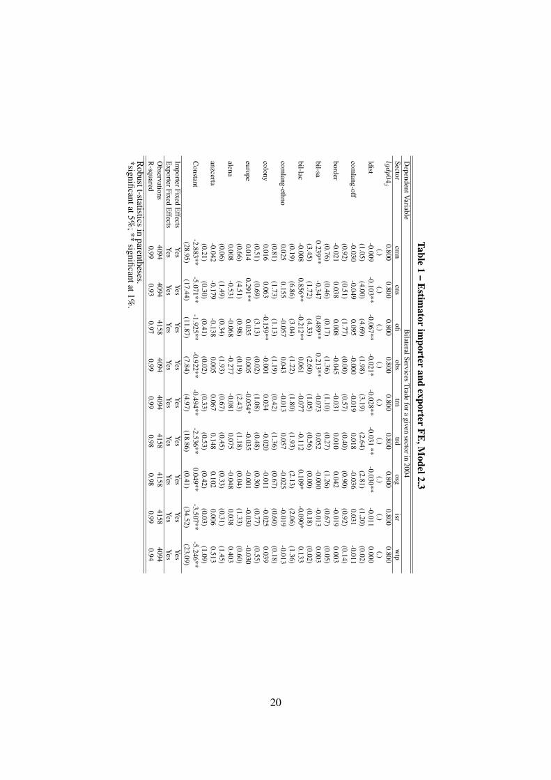
Table1
–E
stimator
importer
andexporter
FE,M
odel2.3D
ependentVariable
BilateralServices
Tradefora
givensectorin
2004Sector
cmn
cnsofi
obstrn
trdosg
isrw
tplgdp04
j0.800
0.8000.800
0.8000.800
0.8000.800
0.8000.800
(.)(.)
(.)(.)
(.)(.)
(.)(.)
(.)ldist
-0.009-0.103**
-0.067**-0.021*
-0.028**-0.031
**-0.030**
-0.0110.000
(1.05)(4.00)
(4.69)(1.98)
(3.19)(2.64)
(2.81)(1.20)
(0.02)com
lang-off-0.030
-0.0490.095
-0.000-0.019
0.018-0.036
0.031-0.011
(0.92)(0.51)
(1.77)(0.00)
(0.57)(0.40)
(0.90)(0.92)
(0.14)border
-0.0210.038
0.008-0.045
-0.0310.010
0.042-0.019
0.003(0.76)
(0.46)(0.17)
(1.36)(1.10)
(0.27)(1.26)
(0.67)(0.05)
bil-sa0.239**
-0.3470.489**
0.213**-0.073
0.052-0.000
-0.0130.003
(3.45)(1.72)
(4.33)(2.60)
(1.05)(0.56)
(0.00)(0.18)
(0.02)bil-lac
-0.0080.856**
-0.212**0.061
-0.077-0.112
0.109*-0.090*
0.133(0.19)
(6.86)(3.04)
(1.22)(1.80)
(1.93)(2.13)
(2.06)(1.36)
comlang-ethno
0.0250.155
-0.0570.043
-0.0130.057
-0.025-0.019
-0.013(0.81)
(1.73)(1.13)
(1.19)(0.42)
(1.36)(0.67)
(0.60)(0.18)
colony0.016
0.063-0.159**
-0.0010.034
-0.020-0.011
-0.0250.039
(0.51)(0.69)
(3.13)(0.02)
(1.08)(0.48)
(0.30)(0.77)
(0.55)europe
0.0140.291**
0.0350.005
-0.054*-0.035
-0.001-0.030
-0.030(0.66)
(4.51)(0.98)
(0.19)(2.43)
(1.18)(0.04)
(1.33)(0.60)
alena0.008
-0.531-0.068
-0.277-0.081
0.075-0.048
0.0380.403
(0.06)(1.49)
(0.34)(1.93)
(0.67)(0.45)
(0.33)(0.31)
(1.45)anzcerta
-0.042-0.179
-0.1380.005
0.0670.148
0.1020.006
0.513(0.21)
(0.30)(0.41)
(0.02)(0.33)
(0.53)(0.42)
(0.03)(1.09)
Constant
-2.883**-5.071**
-1.925**-0.922**
-0.494**-2.536**
0.049**-3.507**
-5.246**(28.95)
(17.44)(11.87)
(7.84)(4.97)
(18.86)(0.41)
(34.52)(23.09)
ImporterFixed
Effects
Yes
Yes
Yes
Yes
Yes
Yes
Yes
Yes
Yes
ExporterFixed
Effects
Yes
Yes
Yes
Yes
Yes
Yes
Yes
Yes
Yes
Observations
40944094
41584094
40944158
41584158
4094R
-squared0.99
0.930.97
0.990.99
0.980.98
0.990.94
Robustt-statistics
inparentheses.
*significantat5%;**
significantat1%.
20
5.2. Considering the zero flows
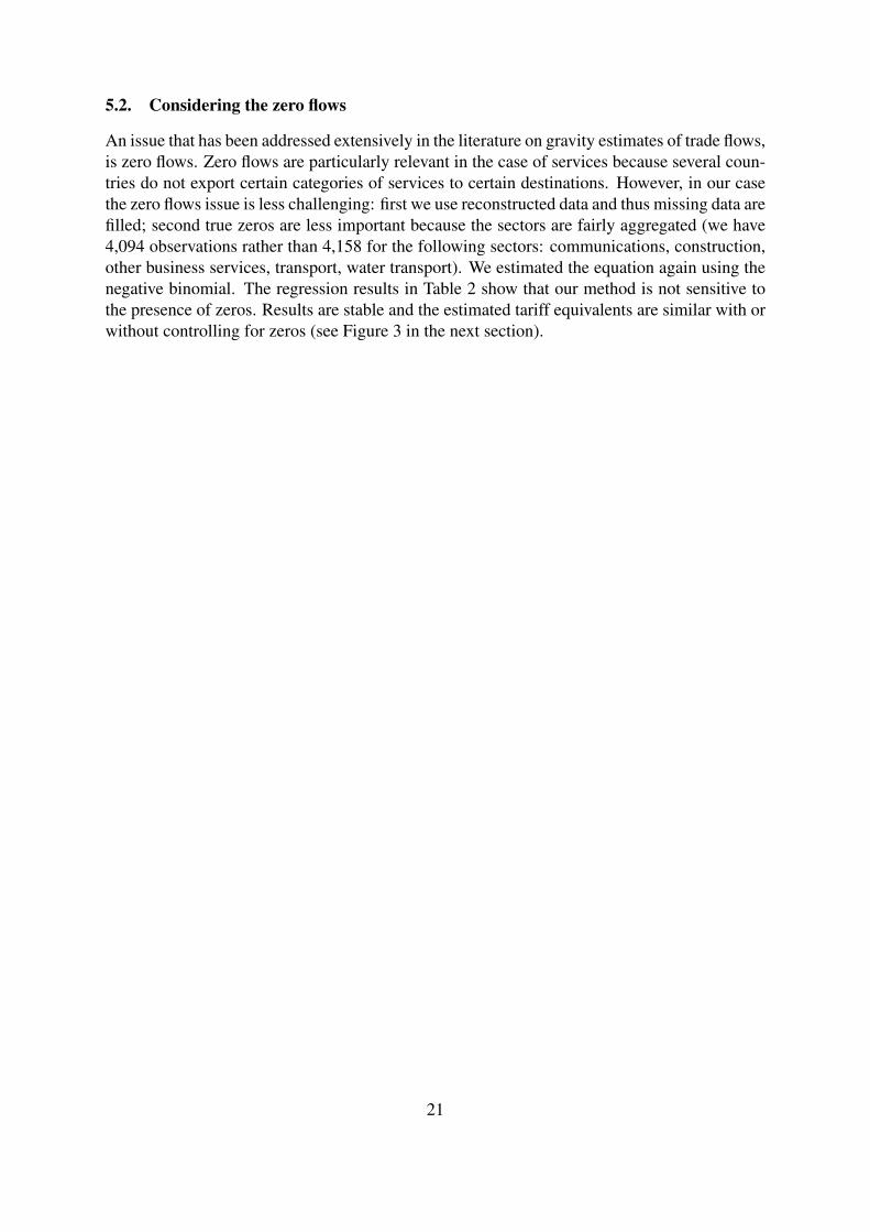
An issue that has been addressed extensively in the literature on gravity estimates of trade flows,is zero flows. Zero flows are particularly relevant in the case of services because several coun-tries do not export certain categories of services to certain destinations. However, in our casethe zero flows issue is less challenging: first we use reconstructed data and thus missing data arefilled; second true zeros are less important because the sectors are fairly aggregated (we have4,094 observations rather than 4,158 for the following sectors: communications, construction,other business services, transport, water transport). We estimated the equation again using thenegative binomial. The regression results in Table 2 show that our method is not sensitive tothe presence of zeros. Results are stable and the estimated tariff equivalents are similar with orwithout controlling for zeros (see Figure 3 in the next section).
21
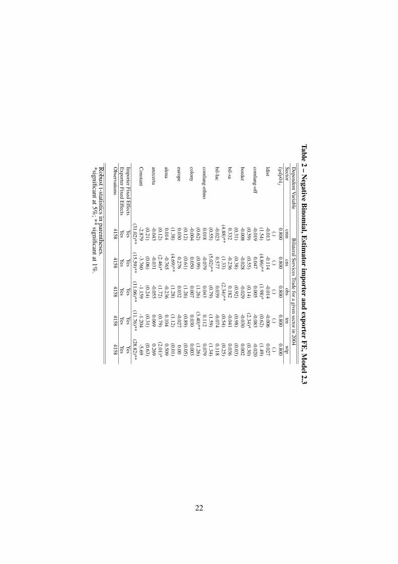
Table2
–N
egativeB
inomial,E
stimator
importer
andexporter
FE,M
odel2.3D
ependentVariable
BilateralServices
Tradefora
givensectorin
2004Sector
cmn
cnsobs
trnw
tplgdp04
j0.800
0.8000.800
0.8000.800
(.)(.)
(.)(.)
(.)ldist
-0.013-0.114
-0.014-0.006
0.027(1.54)
(4.86)**(1.98)*
(0.62)(1.49)
comlang-off
-0.0190.047
0.005-0.083
-0.020(0.59)
(0.55)(0.14)
(2.34)*(0.30)
border-0.008
-0.028-0.029
-0.0300.002
(0.31)(0.38)
(0.92)(0.98)
(0.03)bil-sa
0.332-0.236
0.182-0.041
0.036(4.88)**
(1.33)(2.34)**
(0.54)(0.25)
bil-lac-0.023
0.5770.039
-0.0740.118
(0.55)(5.02)**
(0.79)(1.59)
(1.34)com
lang-ethno0.018
-0.0790.043
0.1120.079
(0.62)(0.99)
(1.26)(3.40)**
(1.26)colony
-0.0040.050
0.0070.030
0.003(0.12)
(0.61)(1.26)
(0.89)(0.05)
europe0.030
0.2760.032
-0.0270.00
(1.38)(4.69)**
(1.28)(1.12)
(0.01)alena
0.014-0.765
-0.2360.104
0.509(0.12)
(2.46)*(1.72)
(0.79)(2.01)*
anzcerta-0.043
-0.031-0.055
0.0690.269
(0.21)(0.06)
(0.24)(0.31)
(0.63)C
onstant-2.879
-3.760-1.159
-1.204-5.69
(31.02)**(15.59)**
(11.06)**(11.76)**
(28.82)**Im
porterFixedE
ffectsY
esY
esY
esY
esY
esE
xporterFixedE
ffectsY
esY
esY
esY
esY
esO
bservations4158
41584158
41584158
Robustt-statistics
inparentheses.
*significantat5%;**
significantat1%.
22
5.3. Regression results from estimations on actual data
We performed panel data estimations for the period 2002-2006, using OECD data, to check thesensitivity of computed AVEs to the presence of reconstructed data in GTAP. Table 3 reports theresults for Total services (200) and for three other subcategories for which the data are available:Transport (205), Communication (245) and Construction (249). The comparison with previousstudies that employ panel data is not straightforward. Firstly samples vary across studies interms of country, time and sectors covered. Secondly, to the best of our knowledge, there isonly one study that estimates trade equations in services including time-varying importer andexporter fixed effects (Head et al., 2007).
Table 3 – Panel estimation with FE (Model 3) using panel OECD dataDependent Variable Bilateral Services Trade (2002-2006)Sector ALL Trn Cmn Cnslgdpjt 0.800 0.800 0.800 0.800
(.) (.) (.) (.)ldist -0.99 -0.97 -1.17 -1.12
(0.02)*** (0.02)*** (0.04)*** (0.07)***cmlng-off 0.48 0.254 0.15 -0.597
(0.04)*** (0.05)*** (0.09) (0.18)***border 0.43 0.25 0.18 -0.31
(0.06)*** (0.07)*** (0.12) (0.18)*colony 1.16 0.74 -0.71 0.34
(0.04)*** (0.06)*** (0.09)*** (0.17)*alena -0.29 -0.56 0 0
(0.27) (0.23)** (0) (0)europe 0.325 0.26 -0.14 0.14
(0.04)*** (0.06)*** (0.13) (0.217)anzcerta 0.59 0.64 0.73 -0.477
(0.11)*** (0.16)*** (0.22)*** (0.66)Constant 22.42 19.27 18.73 17.48
(0.23)*** (0.27)*** (1.05)*** (0.77)***Importer FE Yes Yes Yes YesExporter-Year FE Yes Yes Yes YesYear FE Yes Yes Yes YesObs 16249 7984 3087 2363R-squared 0.82 0.73 0.79 0.72
Robust t-statistics in parentheses.*significant at 10%;**significant at 5%; *** significant at 1%.
Note: Correspondence of sectoral acronyms: trn: transport – cmn: communications – cns: constructions
The picture that emerges from Table 3 is that the gravity equation in panel, even using themore sophisticated fixed effects specifications, is as effective for explaining services trade astrade in goods. We found strong distance effects as in Head et al. (2007) which contrasts withthe results obtained from the fixed effects specifications on cross section data, namely Model2.1, Model 2.2 and Model 2.3, where most of the controls related to gravity-like variables orregional agreements other than distance, are generally not significant. However, the distancevariable might have a different ‘meaning’ in the services sector. In the case of services distanceis also a proxy for omitted variables which are important determinants of trade in services (e.g.cultural and institutional variables).
23
6. TARIFF EQUIVALENTS
The main objective of this paper is estimation of tariff equivalents. In this section we try to as-sess the reliability of the average protection obtained using the GTAP data with the fixed effectmethodology, compared to the full set of estimations from the previous sections. The GTAP isthe largest available source of data on trade in services, both in terms of sectors and countries.Appendix 8.2 reports the AVEs by importing country for the nine services sectors using Model2.3. In a later stage we examine whether alternative strategies lead to different results.
Before commenting on the results note that benchmark countries are either developed countriesor emerging economies such as Hong Kong and Singapore, and (with some exceptions) are thesame across different specifications (Table 4).
Table 4 – Benchmark countries, cross section regressions using GTAP dataSector Model 1.1 Model 1.2 Model 1.3 Model 2.1 Model 2.2 Model 2.3
cmn HKG PHL PHL HKG HKG HKGcns HKG PHL KAZ HKG HKG HKGofi BEL BEL BEL BEL BEL BEL
obs MYS MYS MYS AUT AUT AUTtrn ARG ARG ARG SGP SGP SGPtrd IRL IRL IRL IRL IRL IRL
osg HKG HKG HKG HKG HKG HKGisr MEX MEX MEX
wtp GRC GRC GRC
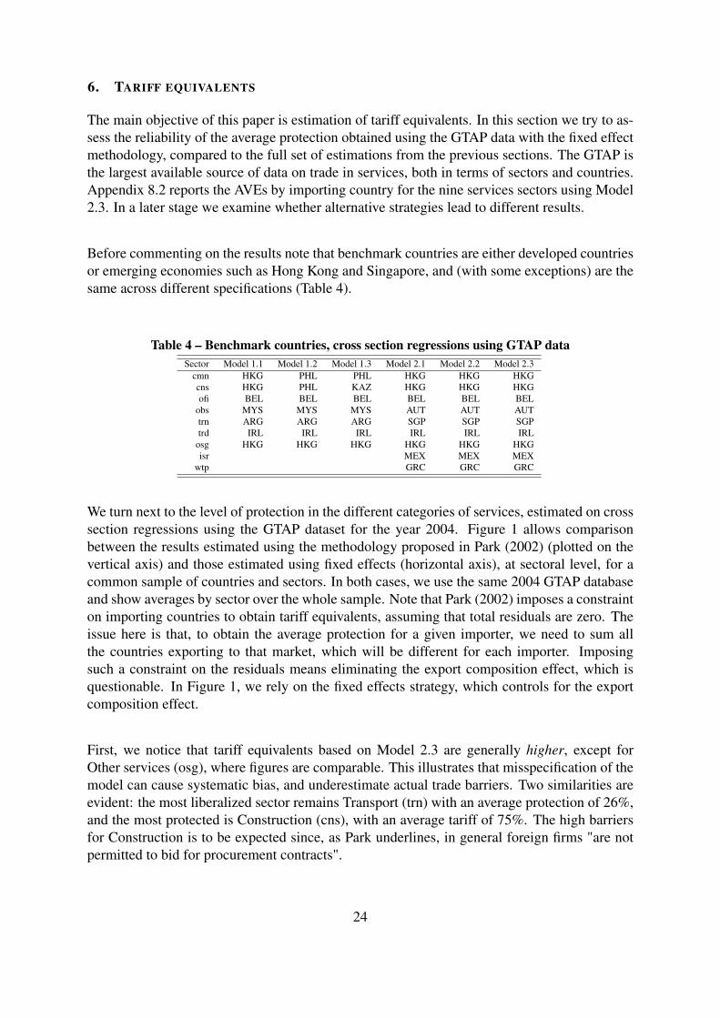
We turn next to the level of protection in the different categories of services, estimated on crosssection regressions using the GTAP dataset for the year 2004. Figure 1 allows comparisonbetween the results estimated using the methodology proposed in Park (2002) (plotted on thevertical axis) and those estimated using fixed effects (horizontal axis), at sectoral level, for acommon sample of countries and sectors. In both cases, we use the same 2004 GTAP databaseand show averages by sector over the whole sample. Note that Park (2002) imposes a constrainton importing countries to obtain tariff equivalents, assuming that total residuals are zero. Theissue here is that, to obtain the average protection for a given importer, we need to sum allthe countries exporting to that market, which will be different for each importer. Imposingsuch a constraint on the residuals means eliminating the export composition effect, which isquestionable. In Figure 1, we rely on the fixed effects strategy, which controls for the exportcomposition effect.
First, we notice that tariff equivalents based on Model 2.3 are generally higher, except forOther services (osg), where figures are comparable. This illustrates that misspecification of themodel can cause systematic bias, and underestimate actual trade barriers. Two similarities areevident: the most liberalized sector remains Transport (trn) with an average protection of 26%,and the most protected is Construction (cns), with an average tariff of 75%. The high barriersfor Construction is to be expected since, as Park underlines, in general foreign firms "are notpermitted to bid for procurement contracts".
24
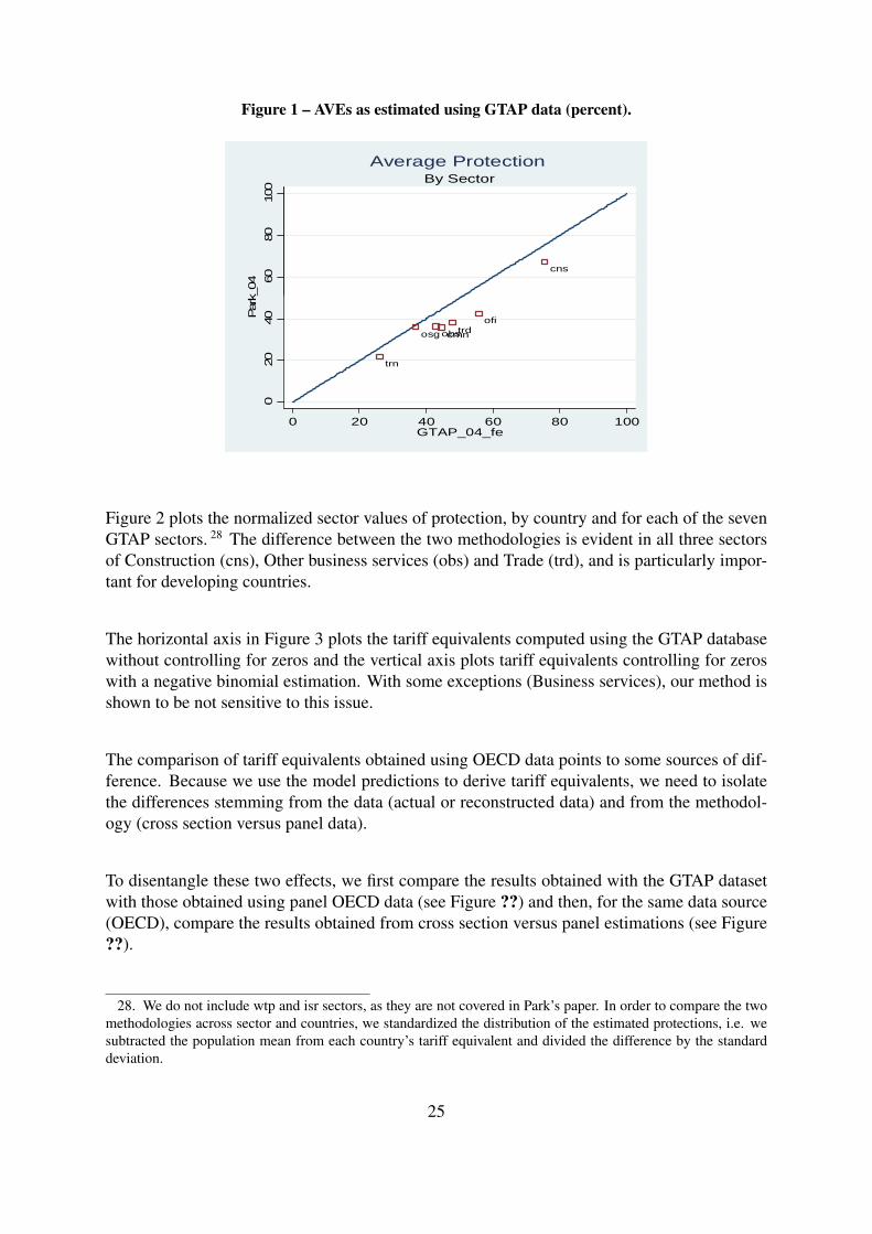
Figure 1 – AVEs as estimated using GTAP data (percent).
cns60
8010
0
Par
k_04
By SectorAverage Protection
cmnobs
ofi
osg trd
trn
020
40
Par
k_04
0 20 40 60 80 100GTAP_04_fe
Figure 2 plots the normalized sector values of protection, by country and for each of the sevenGTAP sectors. 28 The difference between the two methodologies is evident in all three sectorsof Construction (cns), Other business services (obs) and Trade (trd), and is particularly impor-tant for developing countries.
The horizontal axis in Figure 3 plots the tariff equivalents computed using the GTAP databasewithout controlling for zeros and the vertical axis plots tariff equivalents controlling for zeroswith a negative binomial estimation. With some exceptions (Business services), our method isshown to be not sensitive to this issue.
The comparison of tariff equivalents obtained using OECD data points to some sources of dif-ference. Because we use the model predictions to derive tariff equivalents, we need to isolatethe differences stemming from the data (actual or reconstructed data) and from the methodol-ogy (cross section versus panel data).
To disentangle these two effects, we first compare the results obtained with the GTAP datasetwith those obtained using panel OECD data (see Figure ??) and then, for the same data source(OECD), compare the results obtained from cross section versus panel estimations (see Figure??).
28. We do not include wtp and isr sectors, as they are not covered in Park’s paper. In order to compare the twomethodologies across sector and countries, we standardized the distribution of the estimated protections, i.e. wesubtracted the population mean from each country’s tariff equivalent and divided the difference by the standarddeviation.
25
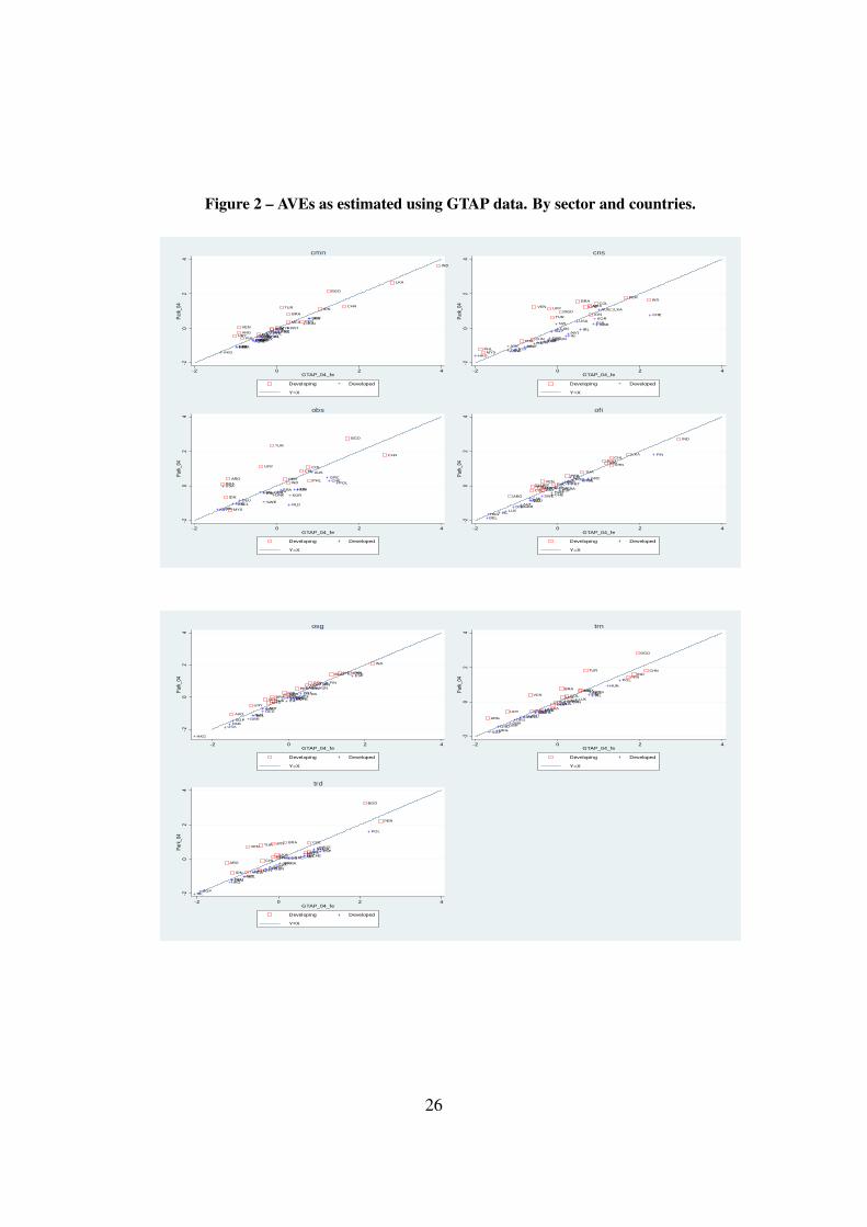
Figure 2 – AVEs as estimated using GTAP data. By sector and countries.
BGD
CHL
PER
THA
TUR
PHL
IDN
IND
LKA
URY
COL
MEX
MYSVEN
ARG
CHN
BRA
CHE
HKG
BEL
AUSNZL
FIN
JPN
KOR IRLSWE
HUN
DNK
POL
SGP
CAN
NLD
PRT
AUT
ESP
GBR
FRAUSA
DEUITA LUXGRC
-20
24
Park
_04
-2 0 2 4GTAP_04_fe
Developing Developed
Y=X
cmn
URY
THA
PHL
INDPER
MYS
CHN
BRA
LKA
COLVEN CHL
TUR
BGDIDN
MEX
ESP
CAN
DNK
PRT
DEU
NZL
NLD
FRA
IRL
GBRUSA
CHE
AUS
SGP
POL
BEL
LUX
HKG
JPN
FIN
SWE
AUT
HUNGRC
ITA
KOR
-20
24
Park
_04
-2 0 2 4GTAP_04_fe
Developing Developed
Y=X
cns
TUR
MYS
URY
ARG
CHL
BRA
BGD
PHL
IDN
COL
CHN
PERIND
HKG
GRC
NLD
AUT
USAFIN
DEU
FRACANESP
AUS
SWEBEL
DNK KOR
CHE
IRL
POL
GBRITA HUN
-20
24
Park
_04
-2 0 2 4GTAP_04_fe
Developing Developed
Y=X
obs
LKA
MYSCOL
ARG
CHL
TUR
IND
PER
URY
THA
IDN
MEX
CHN
VENPHL
BRA
BGD
DEU
HKG
KORAUS
GRCNZL
USASGP
SWE
ESP
NLD
BEL
CHE
IRL
DNK
HUN
JPN
FIN
ITA
AUT
LUX
POLPRT
FRA
GBR
CAN
-20
24
Park
_04
-2 0 2 4GTAP_04_fe
Developing Developed
Y=X
ofi
BRA
COL
VEN
ARG
CHL
BGD
MEX
TURLKA
IDN
CHN
MYSTHA
IND
PER
PHL
URY
LUX
DEU
POL
NLD
JPNNZL
SWEKORITA
DNK
HKG
FRA
GBRSGP
IRL
HUN
BEL
PRT
GRC
CANCHE
FIN
ESP
AUT
AUS
USA
-20
24
Park
_04
-2 0 2 4GTAP_04_fe
Developing Developed
Y=X
osg
IND
BRA
PHL
CHN
BGD
IDN
URY MYS
PER
ARG
VENMEX
LKA
CHL
COL
THA
TUR
HKG
DEU
CHE
PRT
POL
LUX
SWE
AUT
HUN
USA
ITA
IRL
KOR
ESP
FRA
CAN
FIN
NLD
SGP
GBR
BEL
JPNNZL
AUS
DNKGRC
-20
24
Park
_04
-2 0 2 4GTAP_04_fe
Developing Developed
Y=X
trn
CHLPHL
IDN
COLVEN
CHN
LKA
BRA
ARG
MYS
TUR
BGD
MEX
THA
URY
IND
PER
KOR
USA
FRA
DEU
SWE
BEL
PRT
JPN
CHEGRC
SGP
ESP
DNKLUX
POL
AUS
FIN
HKG
AUT
CAN
IRL
GBR
NLD
NZL
ITAHUN
-20
24
Park
_04
-2 0 2 4GTAP_04_fe
Developing Developed
Y=X
trd
26
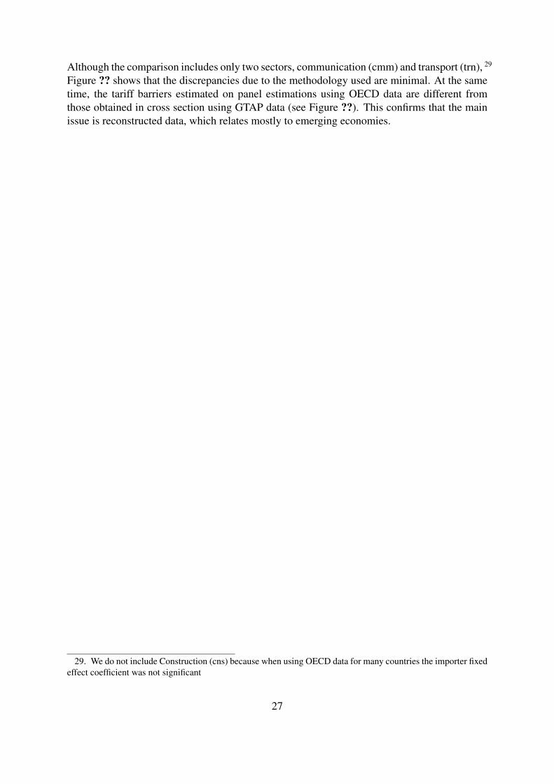
Although the comparison includes only two sectors, communication (cmm) and transport (trn), 29
Figure ?? shows that the discrepancies due to the methodology used are minimal. At the sametime, the tariff barriers estimated on panel estimations using OECD data are different fromthose obtained in cross section using GTAP data (see Figure ??). This confirms that the mainissue is reconstructed data, which relates mostly to emerging economies.
29. We do not include Construction (cns) because when using OECD data for many countries the importer fixedeffect coefficient was not significant
27
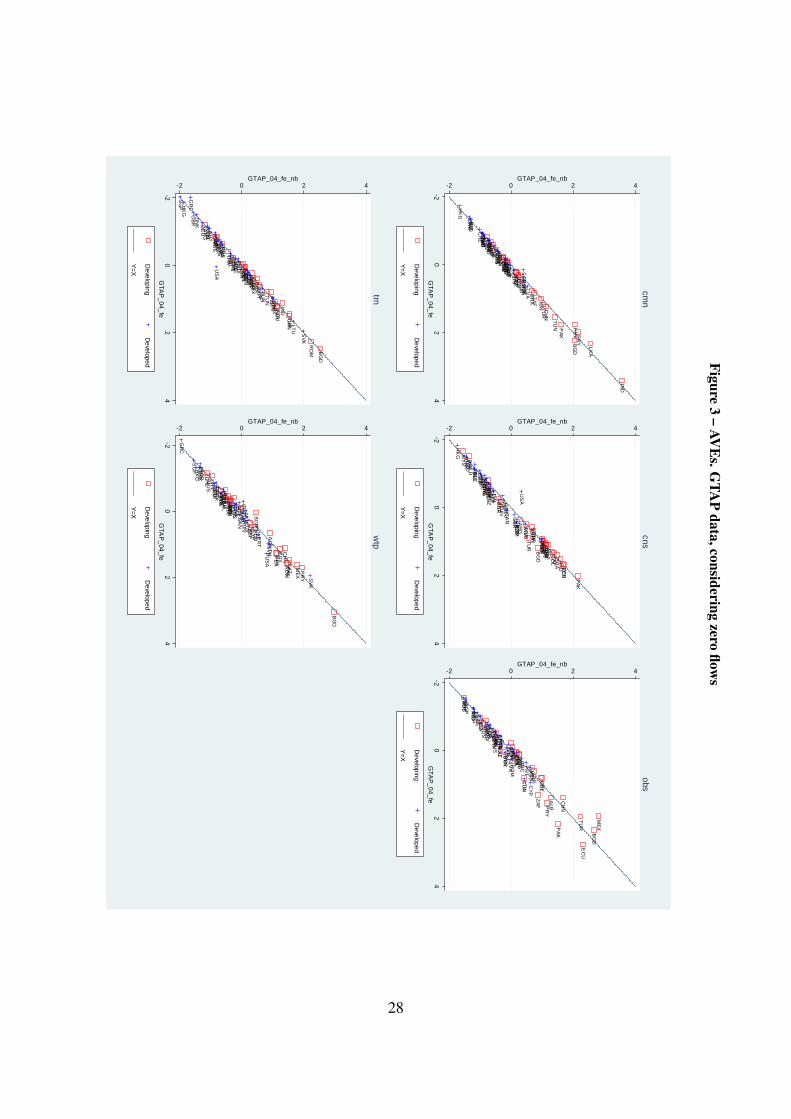
Figure3
–AV
Es.G
TAP
data,consideringzero
flows
TH
A VE
N
KA
Z
CO
L
PA
K
LKA
PH
L
MY
S
PR
Y
AR
G
RO
MM
US
CH
L
BR
A
IND
TU
N
UR
Y
BG
R
PE
RE
GY
RU
SE
CU
HR
V
ME
X
ZA
F IDN C
HN
BG
D
TU
R
ALB C
YP
DN
K
HU
N
AU
T
LTU C
ZE
NZ
L
DE
U
SV
K
PR
T
US
AE
SP
BE
L
ITA
JPN LV
A
IRL
CH
E CA
NG
RC
KO
R
SG
P
NLD
SW
ELU
X FIN
FR
AS
VN
AU
S
GB
R
HK
G
PO
L
ES
T
-2 0 2 4GTAP_04_fe_nb
-20
24
GTA
P_04_fe
Developing
Developed
Y=X
cmn
VE
N
CH
N
IND
PA
K
RO
M
PH
L
AR
G
HR
V
MU
S
BR
AZ
AF
BG
R
TU
R
CO
LP
RY
EG
Y
ALB
RU
S
LKA ME
X
TH
A KG
Z
UR
YC
HL
BG
D
TU
N
PE
R
MY
S
EC
U
IDN
FIN
PO
LF
RA
JPN
ES
P
SV
N
NZ
L
LUX
CZ
E
IRL
GB
R
SW
E GR
C
KO
R
CA
N
DN
K
AU
S
HK
G
HU
N
LTU
US
A
ES
TIT
A
CH
E
DE
U
PR
T
AU
T
CY
P
NLD B
EL
LVA SG
P
SV
K
-2 0 2 4GTAP_04_fe_nb
-20
24
GTA
P_04_fe
Developing
Developed
Y=X
cns
PE
R
TU
R
IND
ZA
F
CH
N
RU
S
MU
S
ME
X
UR
Y
EG
Y
BR
A
PR
Y
BG
R
TH
A
CO
L
EC
U
KA
Z
IDN
TU
NA
RG
BG
D
MY
S
HR
V
ALB
PA
K
PH
L
CH
L
RO
MLK
A
VE
N
LVA
AU
T
HU
N
PR
T
CH
E
LUX
SG
PIR
L
FR
A
AU
S
BE
L
KO
R GB
R
NZ
LJP
NSV
N
CZ
E FIN
HK
G
GR
C
SV
K
DE
US
WE
ES
PE
ST
NLD
CA
N
LTU
ITA
DN
K
US
AP
OL
CY
P
-2 0 2 4GTAP_04_fe_nb
-20
24
GTA
P_04_fe
Developing
Developed
Y=X
obs
TU
N
IND
TU
R
PH
LT
HA
PA
KE
CU
KA
Z
CH
N
AR
G
HR
V
MY
S
IDN
ME
X EG
Y
BG
D
ALB
CH
L
BG
R
MU
SU
RY
PR
Y
RO
M
LKA V
EN
ZA
FB
RA
CO
L
PE
R
RU
S
CA
N
HU
N
SG
P
PO
L
DE
U
US
A
LTU
CZ
E
DN
K
PR
T
JPN
NZ
L
AU
T
SV
K
FIN
SV
N
SW
EF
RA
LVA
ITA
GR
C
ES
T
HK
G
ES
P
GB
R
NLD C
YP
AU
S
IRL
KO
R
LUX
CH
EB
EL
-2 0 2 4GTAP_04_fe_nb
-20
24
GTA
P_04_fe
Developing
Developed
Y=X
trn
IND
BR
A
PE
R
BG
R
CH
N
CH
L
TU
R
BG
D
EC
U
RU
SH
RV
CO
L
MY
S
UR
Y
RO
M
ALB
AR
G
PH
L
MU
S
IDN
KA
Z PR
Y
ZA
F
PA
K
ME
X
VE
NT
UN
TH
ALK
A
EG
Y
PR
T
AU
TC
HE N
LD
LVA
CY
PC
ZE
JPN
LTU
GB
R
DN
K
SV
K
GR
C
AU
S
SG
P
CA
N
FR
A
HK
G
NZ
L
LUX
SW
E
US
A
BE
LP
OL
DE
UIT
AF
IN
HU
N
IRL
ES
P
ES
T
SV
N
KO
R
-2 0 2 4GTAP_04_fe_nb
-20
24
GTA
P_04_fe
Developing
Developed
Y=X
wtp
28
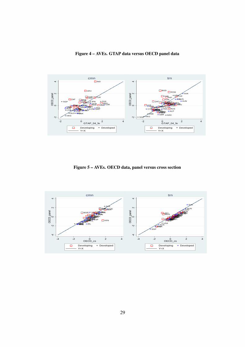
Figure 4 – AVEs. GTAP data versus OECD panel data
ARGBGR
BRA
CHL
CHN
EGY
HRV
IDN
IND
MEXMYS
PHL
ROM
RUSTHA
TUR
VEN
ZAF
AUSAUTCAN
CZE
DEU
ESPEST
FINFRA
GBRGRC
HUN
IRLITA
JPN
KOR
LTU
LUX
LVA
NZL POLPRT
SGP SVK
SVNUSA
02
4O
ECD_
pane
l
cmn
ALB
BGD
BGR
BRA
CHL
CHN
COL
EGY
HRVIDN
IND
LKAMEX
MUSMYS
PAK
PHL
ROM
RUSTHA
TUR
URY
VEN
ZAF
AUS CAN
CHECYP
CZEESPEST
FIN
FRA
HUN
IRL
ITAJPN
LTU
LUXLVA
NLD
NZL
POL
PRT
SVK
SVN
USA
02
4O
ECD_
pane
l
trn
PHL AUT
BEL
CANCHEDEU
DNK
FINGBR
GRC
HKG
IRLITA
KORLUX
NLD
-2
-2 0 2 4GTAP_04_fe
Developing DevelopedY=X
ARG
CHLMUSMYS RUSURY
AUTBELCHE
CYP
DEUDNK
FRA
GBR GRCHKG
KORNLD
SGP
USA
-2
-2 0 2 4GTAP_04_fe
Developing DevelopedY=X
Figure 5 – AVEs. OECD data, panel versus cross section
ARG
BGR
BRA
CHNEGYHRVIDN
IND MEX
MYS
PHL
ROM
RUS
THA
TUR
VEN
AUS
AUT
BELCANCHE
CZE
DEUDNK
ESPESTFIN FRA
GBR
GRCHUN
IRL
ITA
JPNLTU
LVA
NLDNZL
POL
PRTSGP
SVK
SVN
USA
02
4O
ECD_
pane
l
cmn
ARGBGDBGRBRACHN COLEGY
HRV
IDNIND
MEXMUS
PAKPHL
ROMRUS
TURURY
ZAF
AUT
BEL
CZE
DEU
ESPEST
FIN
FRAGBR
GRC
HUN
IRL
ITAJPN
LTULUX
LVA
NLD
POL
PRT
SVK
SVN
USA
02
4O
ECD_
pane
l
trn
AUSHKG IRLNZLSGPUSA
-4-2
-4 -2 0 2 4OECD_cs
Developing DevelopedY=X
LKAAUS
HKG
SGP
USA
-4-2
-4 -2 0 2 4OECD_cs
Developing DevelopedY=X
29
7. CONCLUSION
This research aimed at i) providing tariff equivalents for trade barriers in services based onquantity based methods and ii) assessing the limitations of a method based on gravity and re-constructed data.
We improve on the model proposed in Park (2002) and use a more recent version of the GTAPdataset of trade in services. We obtained tariff equivalents for nine services sectors and 65countries. Some similarities and differences in the level of protection between countries areworth underlining. The least protected countries are the developed economies. The most lib-eralized sector is Transport with an average protection of 26%, and the highest barriers are forConstruction, with an average tariff of 75%.
The second contribution of this paper is to highlight that the misspecification of the gravitymodel used can cause systematic bias and underestimate actual trade barriers. In fact com-pared to Park’s estimates, our tariff equivalents are generally higher, except for Transport andBusiness services where figures are comparable. Relying on OECD panel data for the period2002-2006, the results obtained are different from those obtained using cross section data fromthe GTAP dataset. We showed that those differences are due to the data (reconstructed versusactual), not the methodology (cross section versus panel). This should be taken as warning thatusing partially ’‘reconstructed data’ to estimate tariff equivalents can produce biased results.However, the hierarchy of countries within sectors in terms of protection obtained with thereconstructed data-set is fairly reliable and most divergences related to developing economies.We are therefore quite confident about the accuracy of the tariff equivalents of protection forservices trade proposed here.
It would be useful to compare these results with results from alternative methods for estimatingthe barriers to trade, especially price impact approaches. An example of this approach canbe found in a companion paper Fontagné and Mitaritonna (2009) and is applied to developingeconomies. It highlights that these alternative methods are highly data demanding, which limitstheir use.
30
REFERENCES
Anderson, J. E. (1979). A theoretical foundation for the gravity equation. American EconomicReview, 69(1):106–16.
Anderson, J. E. and van Wincoop, E. (2003). Gravity with Gravitas: A Solution to the BorderPuzzle. American Economic Review, 93(1):170–192.
Baldwin, R. and Taglioni, D. (2006). Gravity for dumies and Dummies for Gravity. WorkingPaper 12516, NBER.
Bergstrand, J. H. (1990). The heckscher-ohlin-samuelson model, the linder hypothesis and thedeterminants of bilateral intra-industry trade. Economic Journal, 100(403):1216–29.
Borchert, I., Gootiz, B., and Mattoo, A. (2011). Restriction on services trade and fdi in devel-oping countries. Technical report, World Bank.
Chen, Z. and Schembri, L. (2002). Measuring the Barriers to Trade in Services: Literature andMethodologies. Trade policy research, Minister of Public Works and Government ServicesCanada.
Deardorff, A. V. (1998). Determinants of Bilateral Trade: Does Gravity Work in a NeoclassicalWorld? In The Regionalization of the World Economy. J.A. Frankel.
Decreux, Y. and Fontagné, L. (2011). Economic Impact of Potential Outcome of the DDA.Working Papers 2011-23, CEPII research center.
Dee, P. (2005). A compendium of barriers to trade in services. Technical report, AustralianNational University. Australian National University.
Dihel, N. and Shepherd, B. (2007). Modal Estimates of Services Barriers. OECD Trade PolicyWorking Papers 51, OECD Trade Directorate.
Feenstra, R. (2002). Border Effects and the Gravity Equation: Consistent Methods for Estima-tion. Scottish Journal of Political Economy, 49(5):491–506.
Feenstra, R. (2004). Advanced International Trade: Theory and Evidence. Princeton UniversityPress.
Fontagné, L. and Mitaritonna, C. (2009). Assessing Barriers to Trade in the Distribution andTelecom Sectors in Emerging Countries. Technical report, CEPII research center.
Francois, J. (1993). Explaining the Pattern of Trade in Producer Services. International Eco-nomic Journal, 7(3):23–31.
Francois, J., Pindyuk, O., and Woerz, J. (2009). Trends in International Trade and FDI inServices: a global dataset of services trade. Technical Report Discussion paper 2009-08-02,Institute for International and Development Economics.
Francois, J., van Meijl, H., and van Tongeren, F. (2005). Trade liberalization in the DohaDevelopment Round. Economic Policy, 20(42):349–391.
Gootiiz, B. and Mattoo, A. (2009). Services in Doha. What’s on the table? World bank PolicyResearch Paper, 4903.
Head, K., Mayer, T., and Ries, J. (2007). How Remote is the Offshoring Threat? WorkingPaper 18, CEPII.
Helpman, E. and Krugman, P. (1985). Market Structure and Foreign Trade. Cambridge Uni-versity Press.
31
Helpman, E., Melitz, M., and Rubinstein, Y. (2007). Estimating Trade Flows: Trading Part-ners and Trading Volumes. NBER Working Papers 12927, National Bureau of EconomicResearch, Inc.
Hoekman, B. (1996). Assessing the General Agreement on Trade in Services. In The UruguayRound and the Developing Countries. Cambridge University Press.
Kimura, F. and Lee, H.-H. (2006). The Gravity Equation in International Trade in Services.Review of World Economics, 142(1):92–121.
Kox, H. L. and Nordas, H. K. (2007). Services trade and domestic regulation. MPRA Paper2116, University Library of Munich, Germany.
Mattoo, A., Rathindran, R., and Subramanian, A. (2001). Measuring services trade liberaliza-tion and its impact on economic growth: an illustration. Policy Research Working PaperSeries 2655, The World Bank.
Melitz, M. J. and Ottaviano, G. I. P. (2008). Market size, trade, and productivity. Review ofEconomic Studies, 75(1):295–316.
Mirza, D. and Nicoletti, G. (2004). What’s so Special about Trade in Services? Research Paper2004/02, Leverhulme Centre for Research on Globalisation and Economic Policy.
Park, S.-C. (2002). Measuring Tariff Equivalents in Cross-Border Trade in Services. TradeWorking Papers 353, East Asian Bureau of Economic Research.
Stern, R. M. (2000). Quantifying Barriers to Trade in Services. Working Papers 470, ResearchSeminar in International Economics, University of Michigan.
van Leeuwen, N. and Lejour, A. (2008). The quality of bilateral services trade data. Cpbmemoranda, CPB Netherlands Bureau for Economic Policy Analysis.
Walsh, K. (2006). Trade in Services: Does Gravity Hold? A Gravity Model Approach toEstimating Barriers to Services Trade. The Institute for International Integration StudiesDiscussion Paper Series 183, IIIS.
World-Trade-Organization (2010). World Trade Report.
32
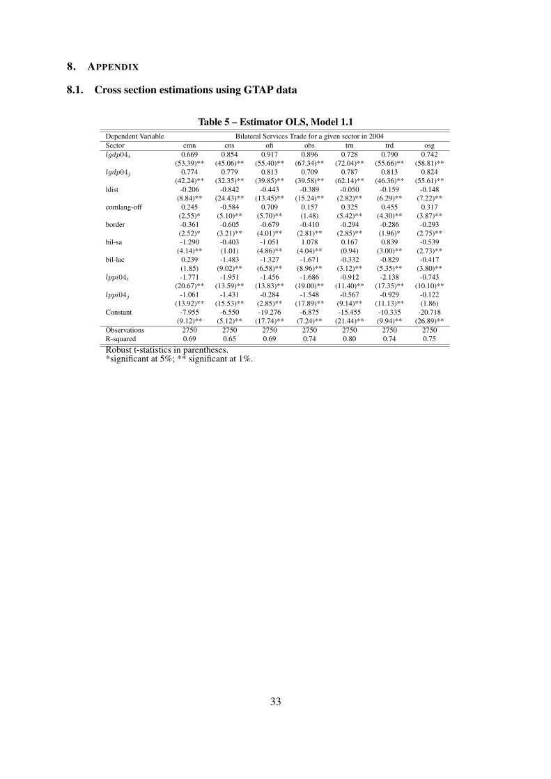
8. APPENDIX
8.1. Cross section estimations using GTAP data
Table 5 – Estimator OLS, Model 1.1Dependent Variable Bilateral Services Trade for a given sector in 2004Sector cmn cns ofi obs trn trd osglgdp04i 0.669 0.854 0.917 0.896 0.728 0.790 0.742
(53.39)** (45.06)** (55.40)** (67.34)** (72.04)** (55.66)** (58.81)**lgdp04j 0.774 0.779 0.813 0.709 0.787 0.813 0.824
(42.24)** (32.35)** (39.85)** (39.58)** (62.14)** (46.36)** (55.61)**ldist -0.206 -0.842 -0.443 -0.389 -0.050 -0.159 -0.148
(8.84)** (24.43)** (13.45)** (15.24)** (2.82)** (6.29)** (7.22)**comlang-off 0.245 -0.584 0.709 0.157 0.325 0.455 0.317
(2.55)* (5.10)** (5.70)** (1.48) (5.42)** (4.30)** (3.87)**border -0.361 -0.605 -0.679 -0.410 -0.294 -0.286 -0.293
(2.52)* (3.21)** (4.01)** (2.81)** (2.85)** (1.96)* (2.75)**bil-sa -1.290 -0.403 -1.051 1.078 0.167 0.839 -0.539
(4.14)** (1.01) (4.86)** (4.04)** (0.94) (3.00)** (2.73)**bil-lac 0.239 -1.483 -1.327 -1.671 -0.332 -0.829 -0.417
(1.85) (9.02)** (6.58)** (8.96)** (3.12)** (5.35)** (3.80)**lppi04i -1.771 -1.951 -1.456 -1.686 -0.912 -2.138 -0.743
(20.67)** (13.59)** (13.83)** (19.00)** (11.40)** (17.35)** (10.10)**lppi04j -1.061 -1.431 -0.284 -1.548 -0.567 -0.929 -0.122
(13.92)** (15.53)** (2.85)** (17.89)** (9.14)** (11.13)** (1.86)Constant -7.955 -6.550 -19.276 -6.875 -15.455 -10.335 -20.718
(9.12)** (5.12)** (17.74)** (7.24)** (21.44)** (9.94)** (26.89)**Observations 2750 2750 2750 2750 2750 2750 2750R-squared 0.69 0.65 0.69 0.74 0.80 0.74 0.75
Robust t-statistics in parentheses.*significant at 5%; ** significant at 1%.
33
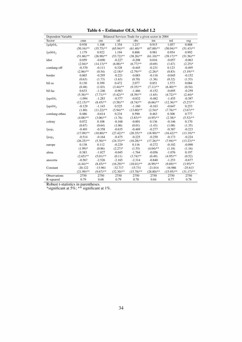
Table 6 – Estimator OLS, Model 1.2Dependent Variable Bilateral Services Trade for a given sector in 2004Sector cmn cns ofi obs trn trd osglgdp04i 0.938 1.108 1.354 1.217 0.915 1.057 0.888
(50.16)** (35.75)** (65.94)** (61.40)** (67.00)** (50.94)** (51.43)**lpib04j 1.179 0.922 1.194 0.888 0.981 0.954 0.992
(51.86)** (26.90)** (53.72)** (38.26)** (61.10)** (39.17)** (51.56)**ldist 0.059 -0.690 -0.227 -0.208 0.016 -0.057 -0.063
(2.04)* (14.13)** (6.88)** (6.77)** (0.69) (1.67) (2.25)*comlang-off -0.370 -0.111 0.328 -0.445 -0.231 0.123 -0.495
(2.86)** (0.54) (2.18)* (2.79)** (2.26)* (0.83) (3.19)**border 0.065 -0.295 -0.221 -0.083 -0.116 -0.045 -0.152
(0.63) (1.73) (1.63) (0.70) (1.36) (0.32) (1.53)bil-sa 0.130 0.399 0.472 2.077 0.851 1.573 0.084
(0.48) (1.03) (3.44)** (9.35)** (7.11)** (6.40)** (0.54)bil-lac 0.633 -1.246 -0.963 -1.466 -0.152 -0.695 -0.259
(5.36)** (7.71)** (5.42)** (8.39)** (1.65) (4.72)** (2.44)*lppi04i -1.094 -1.283 -0.377 -0.832 -0.482 -1.455 -0.387
(12.15)** (8.45)** (3.58)** (8.74)** (6.66)** (12.36)** (5.27)**lppi04j -0.129 -1.143 0.525 -1.160 -0.163 -0.647 0.253
(1.80) (11.22)** (5.94)** (13.60)** (2.54)* (7.76)** (3.67)**comlang-ethno 0.486 -0.614 0.234 0.590 0.463 0.308 0.777
(4.08)** (3.06)** (1.76) (3.83)** (4.95)** (2.38)* (5.52)**colony 0.072 0.108 -0.168 -0.001 0.136 -0.146 0.170
(0.67) (0.64) (1.06) (0.01) (1.43) (1.08) (1.35)lpopi -0.401 -0.358 -0.635 -0.469 -0.277 -0.387 -0.223
(17.09)** (10.80)** (27.42)** (20.35)** (18.90)** (16.42)** (13.19)**lpopj -0.514 -0.164 -0.475 -0.225 -0.250 -0.173 -0.224
(26.25)** (5.30)** (24.33)** (10.28)** (17.26)** (7.94)** (13.23)**europe 0.138 0.112 -0.229 0.116 -0.272 -0.102 -0.090
(1.99)* (0.86) (2.27)* (1.55) (4.04)** (1.18) (1.16)alena 0.383 -1.827 -0.045 -1.764 -0.056 -1.076 0.197
(2.65)** (5.01)** (0.11) (3.74)** (0.49) (4.95)** (0.52)anzcerta -0.567 -2.526 -2.165 -2.314 -0.840 -1.253 -0.677
(4.44)** (8.45)** (16.29)** (18.01)** (6.99)** (9.69)** (3.95)**Constant -20.122 -13.961 -32.717 -15.731 -21.014 -16.986 -25.613
(21.99)** (9.67)** (32.30)** (15.78)** (28.80)** (15.95)** (31.17)**Observations 2750 2750 2750 2750 2750 2750 2750R-squared 0.79 0.68 0.79 0.78 0.84 0.77 0.78
Robust t-statistics in parentheses.*significant at 5%; ** significant at 1%.
34
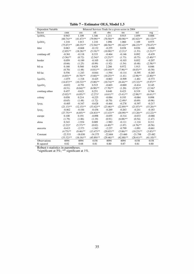
Table 7 – Estimator OLS, Model 1.3Dependent Variable Bilateral Services Trade for a given sector in 2004Sector cmn cns ofi obs trn trd osglpib04i 0.943 1.109 1.346 1.211 0.915 1.059 0.888
(60.74)** (41.67)** (79.99)** (70.50)** (80.98)** (63.82)** (61.12)**lpib04j 1.210 1.013 1.210 1.096 1.060 1.109 0.975
(75.07)** (40.35)** (72.94)** (60.56)** (92.42)** (66.23)** (70.47)**ldist 0.063 -0.668 -0.132 -0.255 0.038 0.036 -0.068
(2.85)** (18.28)** (5.19)** (10.90)** (2.21)* (1.53) (3.21)**comlang-off -0.361 -0.118 0.333 -0.464 -0.146 0.092 -0.439
(3.56)** (0.72) (2.54)* (3.23)** (1.73) (0.75) (3.40)**border 0.059 -0.189 -0.105 -0.183 -0.103 0.052 -0.207
(0.66) (1.25) (0.99) (1.92) (1.54) (0.48) (2.58)**bil-sa 0.188 0.560 0.629 2.286 0.972 1.913 0.046
(0.70) (1.48) (4.81)** (10.44)** (7.96)** (8.03)** (0.30)bil-lac 0.556 -1.243 -0.844 -1.594 -0.114 -0.395 -0.265
(4.85)** (8.70)** (5.60)** (10.25)** (1.41) (2.98)** (2.80)**lppi04i -1.075 -1.318 -0.425 -0.863 -0.509 -1.461 -0.373
(14.67)** (10.32)** (5.00)** (10.74)** (8.44)** (15.32)** (5.97)**lppi04j -0.032 -0.791 0.515 -0.603 -0.069 -0.414 0.145
(0.51) (8.84)** (6.90)** (7.70)** (1.20) (5.92)** (2.34)*comlang-ethno 0.457 -0.621 0.251 0.640 0.423 0.319 0.766
(5.02)** (4.05)** (2.27)* (4.61)** (5.41)** (2.98)** (6.61)**colony 0.058 0.214 -0.225 -0.084 0.193 -0.084 0.098
(0.65) (1.48) (1.72) (0.70) (2.49)* (0.69) (0.96)lpopi -0.405 -0.347 -0.628 -0.464 -0.278 -0.397 -0.217
(21.13)** (12.15)** (33.42)** (23.46)** (22.89)** (21.07)** (15.26)**lpopj -0.462 -0.184 -0.436 -0.269 -0.263 -0.241 -0.183
(27.75)** (6.85)** (24.83)** (13.43)** (20.99)** (13.20)** (12.22)**europe 0.100 0.191 -0.098 -0.055 -0.314 -0.033 -0.088
(1.79) (1.86) (1.19) (0.91) (6.08)** (0.54) (1.47)alena 0.343 -1.934 0.009 -1.982 -0.111 -1.124 0.211
(2.22)* (5.37)** (0.02) (4.40)** (1.07) (4.76)** (0.56)anzcerta -0.413 -2.373 -1.943 -2.237 -0.799 -1.091 -0.661
(4.75)** (9.46)** (13.47)** (20.65)** (5.06)** (10.23)** (3.83)**Constant -22.533 -18.030 -34.375 -22.604 -23.460 -21.798 -25.482
(33.32)** (16.16)** (45.89)** (29.46)** (42.88)** (28.41)** (41.10)**Observations 4094 4094 4158 4094 4094 4158 4158R-squared 0.82 0.68 0.81 0.80 0.87 0.81 0.80
Robust t-statistics in parentheses.*significant at 5%; ** significant at 1%.
35
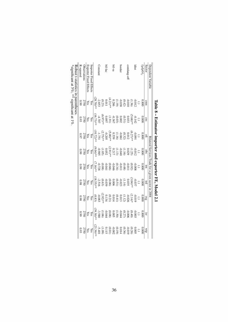
Table8
–E
stimator
importer
andexporter
FE,M
odel2.1D
ependentVariable
BilateralServices
Tradefora
givensectorin
2004Sector
cmn
cnsofi
obstrn
trdosg
isrw
tplgdp04
j0.800
0.8000.800
0.8000.800
0.8000.800
0.8000.800
(.)(.)
(.)(.)
(.)(.)
(.)(.)
(.)ldist
-0.012-0.142
-0.091-0.012
-0.008-0.037
-0.019-0.003
0.005(1.36)
(5.68)**(6.27)**
(1.25)(0.92)
(3.04)**(2.14)*
(0.40)(0.26)
comlang-off
-0.0100.033
0.0120.029
-0.0110.035
-0.026-0.006
-0.019(0.42)
(0.51)(0.32)
(1.16)(0.48)
(1.14)(1.12)
(0.27)(0.36)
border-0.038
0.002-0.061
-0.040-0.011
-0.0230.013
-0.0440.014
(1.19)(0.03)
(1.16)(1.13)
(0.34)(0.51)
(0.41)(1.50)
(0.19)bil-sa
0.286-0.367
0.5590.217
-0.0460.006
0.0140.005
-0.002(4.21)**
(1.91)(5.00)**
(2.91)**(0.66)
(0.06)(0.21)
(0.08)(0.01)
bil-lac0.011
0.897-0.205
0.052-0.041
-0.0390.134
-0.0440.115
(0.23)(6.97)**
(2.75)**(1.05)
(0.88)(0.63)
(2.92)**(1.06)
(1.09)C
onstant-2.853
-4.707-1.751
-0.985-0.728
-2.516-0.083
-3.580-5.401
(28.70)**(16.73)**
(10.72)**(9.04)**
(7.16)**(18.55)**
(0.83)(39.30)**
(23.39)**Im
porterFixedE
ffectsY
esY
esY
esY
esY
esY
esY
esY
esY
esE
xporterFixedE
ffectsY
esY
esY
esY
esY
esY
esY
esY
esY
esO
bservations2750
27502750
27502750
27502750
27502750
R-squared
0.990.93
0.970.99
0.990.98
0.980.99
0.93
Robustt-statistics
inparentheses.
*significantat5%;**
significantat1%.
36
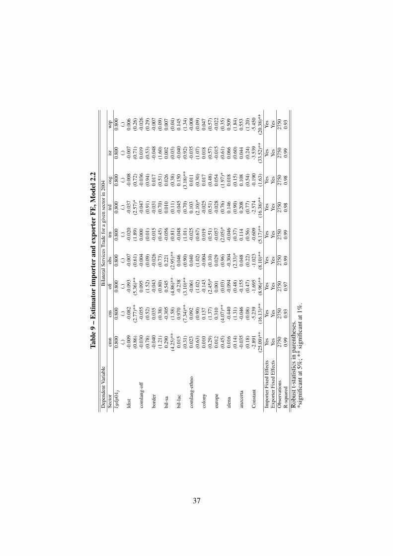
Tabl
e9
–E
stim
ator
impo
rter
and
expo
rter
FE,M
odel
2.2
Dep
ende
ntV
aria
ble
Bila
tera
lSer
vice
sTr
ade
fora
give
nse
ctor
in20
04Se
ctor
cmn
cns
ofiob
str
ntr
dos
gis
rw
tplgdp04
j0.
800
0.80
00.
800
0.80
00.
800
0.80
00.
800
0.80
00.
800
(.)(.)
(.)(.)
(.)(.)
(.)(.)
(.)ld
ist
-0.0
09-0
.082
-0.0
93-0
.007
-0.0
20-0
.037
-0.0
08-0
.007
0.00
6(0
.86)
(2.7
7)**
(5.3
6)**
(0.6
1)(1
.89)
(2.5
7)*
(0.7
2)(0
.71)
(0.2
6)co
mla
ng-o
ff-0
.030
-0.0
550.
095
-0.0
040.
000
-0.0
47-0
.036
0.01
9-0
.026
(0.7
8)(0
.52)
(1.5
2)(0
.09)
(0.0
1)(0
.91)
(0.9
4)(0
.53)
(0.2
9)bo
rder
-0.0
400.
035
-0.0
43-0
.026
-0.0
15-0
.031
0.01
7-0
.048
-0.0
07(1
.21)
(0.3
8)(0
.80)
(0.7
3)(0
.45)
(0.7
0)(0
.51)
(1.6
0)(0
.09)
bil-
sa0.
290
-0.3
050.
545
0.22
1-0
.056
0.01
00.
026
0.00
20.
007
(4.2
5)**
(1.5
8)(4
.86)
**(2
.95)
**(0
.81)
(0.1
1)(0
.38)
(0.0
3)(0
.04)
bil-
lac
0.01
50.
970
-0.2
380.
046
-0.0
48-0
.045
0.15
0-0
.040
0.14
5(0
.31)
(7.3
4)**
(3.1
0)**
(0.9
0)(1
.01)
(0.7
0)(3
.18)
**(0
.92)
(1.3
4)co
mla
ng-e
thno
0.02
30.
092
-0.0
610.
040
-0.0
250.
103
0.01
1-0
.035
-0.0
08(0
.63)
(0.9
0)(1
.02)
(1.0
2)(0
.67)
(2.1
0)*
(0.3
0)(1
.07)
(0.0
9)co
lony
0.01
00.
137
-0.1
43-0
.004
0.01
9-0
.025
0.01
70.
018
0.04
7(0
.29)
(1.3
7)(2
.45)
*(0
.10)
(0.5
1)(0
.51)
(0.4
8)(0
.57)
(0.5
7)eu
rope
0.01
20.
310
0.00
10.
029
-0.0
57-0
.028
0.05
4-0
.015
-0.0
22(0
.45)
(4.0
7)**
(0.0
3)(0
.96)
(2.0
5)*
(0.7
6)(1
.97)
*(0
.61)
(0.3
5)al
ena
0.01
6-0
.440
-0.0
94-0
.304
-0.0
460.
146
0.01
80.
066
0.50
9(0
.14)
(1.3
1)(0
.48)
(2.3
3)*
(0.3
7)(0
.90)
(0.1
5)(0
.60)
(1.8
4)an
zcer
ta-0
.035
-0.0
46-0
.155
0.04
80.
114
0.20
80.
108
0.04
40.
553
(0.1
8)(0
.08)
(0.4
7)(0
.22)
(0.5
6)(0
.77)
(0.5
4)(0
.24)
(1.2
0)C
onst
ant
-2.8
91-5
.239
-1.6
95-1
.023
-0.6
09-2
.574
-0.1
90-3
.539
-5.4
50(2
5.09
)**
(16.
13)*
*(8
.96)
**(8
.10)
**(5
.17)
**(1
6.38
)**
(1.6
3)(3
3.52
)**
(20.
38)*
*Im
port
erFi
xed
Eff
ects
Yes
Yes
Yes
Yes
Yes
Yes
Yes
Yes
Yes
Exp
orte
rFix
edE
ffec
tsY
esY
esY
esY
esY
esY
esY
esY
esY
esO
bser
vatio
ns27
5027
5027
5027
5027
5027
5027
5027
5027
50R
-squ
ared
0.99
0.93
0.97
0.99
0.99
0.98
0.98
0.99
0.93
Rob
ustt
-sta
tistic
sin
pare
nthe
ses.
*sig
nific
anta
t5%
;**
sign
ifica
ntat
1%.
37
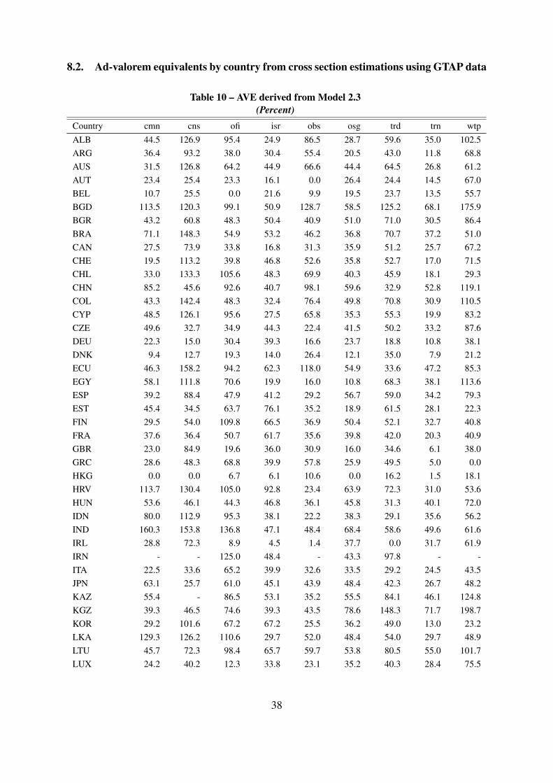
8.2. Ad-valorem equivalents by country from cross section estimations using GTAP data
Table 10 – AVE derived from Model 2.3(Percent)
Country cmn cns ofi isr obs osg trd trn wtpALB 44.5 126.9 95.4 24.9 86.5 28.7 59.6 35.0 102.5ARG 36.4 93.2 38.0 30.4 55.4 20.5 43.0 11.8 68.8AUS 31.5 126.8 64.2 44.9 66.6 44.4 64.5 26.8 61.2AUT 23.4 25.4 23.3 16.1 0.0 26.4 24.4 14.5 67.0BEL 10.7 25.5 0.0 21.6 9.9 19.5 23.7 13.5 55.7BGD 113.5 120.3 99.1 50.9 128.7 58.5 125.2 68.1 175.9BGR 43.2 60.8 48.3 50.4 40.9 51.0 71.0 30.5 86.4BRA 71.1 148.3 54.9 53.2 46.2 36.8 70.7 37.2 51.0CAN 27.5 73.9 33.8 16.8 31.3 35.9 51.2 25.7 67.2CHE 19.5 113.2 39.8 46.8 52.6 35.8 52.7 17.0 71.5CHL 33.0 133.3 105.6 48.3 69.9 40.3 45.9 18.1 29.3CHN 85.2 45.6 92.6 40.7 98.1 59.6 32.9 52.8 119.1COL 43.3 142.4 48.3 32.4 76.4 49.8 70.8 30.9 110.5CYP 48.5 126.1 95.6 27.5 65.8 35.3 55.3 19.9 83.2CZE 49.6 32.7 34.9 44.3 22.4 41.5 50.2 33.2 87.6DEU 22.3 15.0 30.4 39.3 16.6 23.7 18.8 10.8 38.1DNK 9.4 12.7 19.3 14.0 26.4 12.1 35.0 7.9 21.2ECU 46.3 158.2 94.2 62.3 118.0 54.9 33.6 47.2 85.3EGY 58.1 111.8 70.6 19.9 16.0 10.8 68.3 38.1 113.6ESP 39.2 88.4 47.9 41.2 29.2 56.7 59.0 34.2 79.3EST 45.4 34.5 63.7 76.1 35.2 18.9 61.5 28.1 22.3FIN 29.5 54.0 109.8 66.5 36.9 50.4 52.1 32.7 40.8FRA 37.6 36.4 50.7 61.7 35.6 39.8 42.0 20.3 40.9GBR 23.0 84.9 19.6 36.0 30.9 16.0 34.6 6.1 38.0GRC 28.6 48.3 68.8 39.9 57.8 25.9 49.5 5.0 0.0HKG 0.0 0.0 6.7 6.1 10.6 0.0 16.2 1.5 18.1HRV 113.7 130.4 105.0 92.8 23.4 63.9 72.3 31.0 53.6HUN 53.6 46.1 44.3 46.8 36.1 45.8 31.3 40.1 72.0IDN 80.0 112.9 95.3 38.1 22.2 38.3 29.1 35.6 56.2IND 160.3 153.8 136.8 47.1 48.4 68.4 58.6 49.6 61.6IRL 28.8 72.3 8.9 4.5 1.4 37.7 0.0 31.7 61.9IRN - - 125.0 48.4 - 43.3 97.8 - -ITA 22.5 33.6 65.2 39.9 32.6 33.5 29.2 24.5 43.5JPN 63.1 25.7 61.0 45.1 43.9 48.4 42.3 26.7 48.2KAZ 55.4 - 86.5 53.1 35.2 55.5 84.1 46.1 124.8KGZ 39.3 46.5 74.6 39.3 43.5 78.6 148.3 71.7 198.7KOR 29.2 101.6 67.2 67.2 25.5 36.2 49.0 13.0 23.2LKA 129.3 126.2 110.6 29.7 52.0 48.4 54.0 29.7 48.9LTU 45.7 72.3 98.4 65.7 59.7 53.8 80.5 55.0 101.7LUX 24.2 40.2 12.3 33.8 23.1 35.2 40.3 28.4 75.5
38
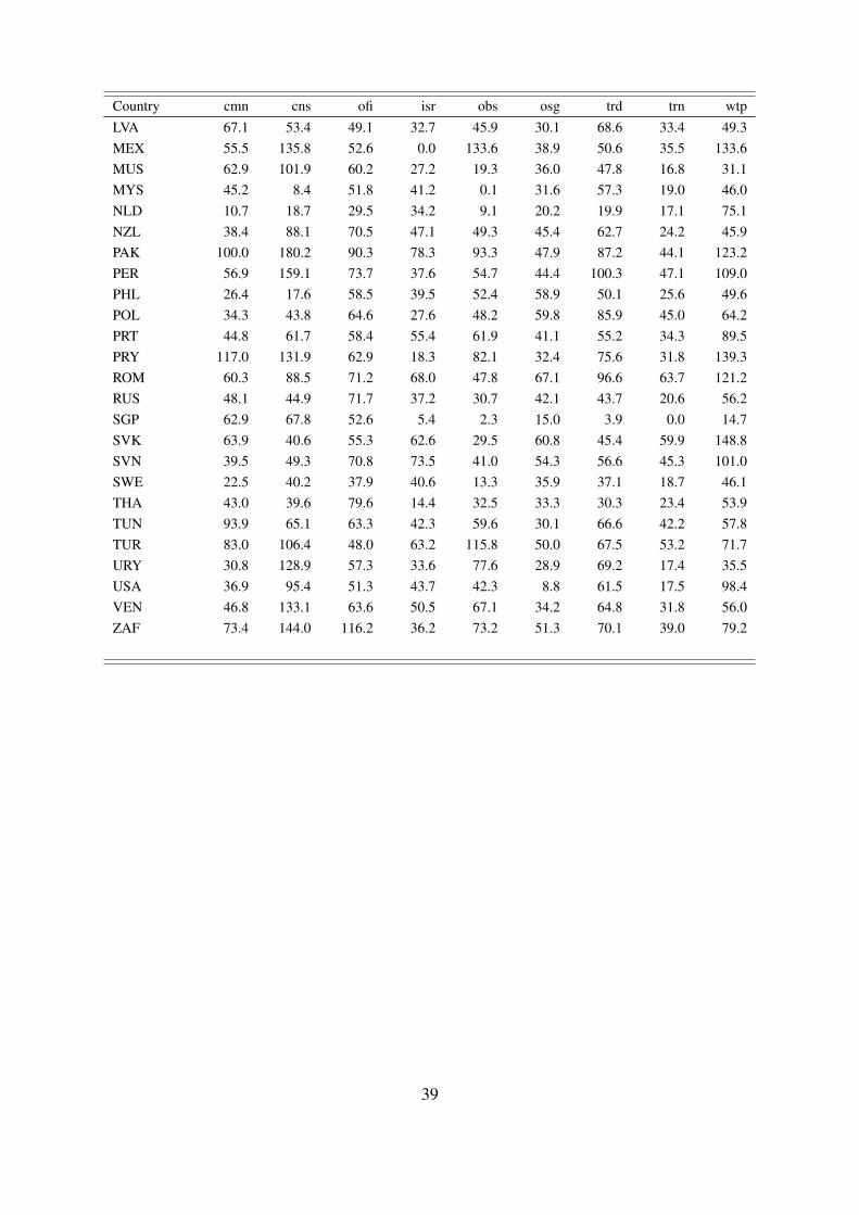
Country cmn cns ofi isr obs osg trd trn wtpLVA 67.1 53.4 49.1 32.7 45.9 30.1 68.6 33.4 49.3MEX 55.5 135.8 52.6 0.0 133.6 38.9 50.6 35.5 133.6MUS 62.9 101.9 60.2 27.2 19.3 36.0 47.8 16.8 31.1MYS 45.2 8.4 51.8 41.2 0.1 31.6 57.3 19.0 46.0NLD 10.7 18.7 29.5 34.2 9.1 20.2 19.9 17.1 75.1NZL 38.4 88.1 70.5 47.1 49.3 45.4 62.7 24.2 45.9PAK 100.0 180.2 90.3 78.3 93.3 47.9 87.2 44.1 123.2PER 56.9 159.1 73.7 37.6 54.7 44.4 100.3 47.1 109.0PHL 26.4 17.6 58.5 39.5 52.4 58.9 50.1 25.6 49.6POL 34.3 43.8 64.6 27.6 48.2 59.8 85.9 45.0 64.2PRT 44.8 61.7 58.4 55.4 61.9 41.1 55.2 34.3 89.5PRY 117.0 131.9 62.9 18.3 82.1 32.4 75.6 31.8 139.3ROM 60.3 88.5 71.2 68.0 47.8 67.1 96.6 63.7 121.2RUS 48.1 44.9 71.7 37.2 30.7 42.1 43.7 20.6 56.2SGP 62.9 67.8 52.6 5.4 2.3 15.0 3.9 0.0 14.7SVK 63.9 40.6 55.3 62.6 29.5 60.8 45.4 59.9 148.8SVN 39.5 49.3 70.8 73.5 41.0 54.3 56.6 45.3 101.0SWE 22.5 40.2 37.9 40.6 13.3 35.9 37.1 18.7 46.1THA 43.0 39.6 79.6 14.4 32.5 33.3 30.3 23.4 53.9TUN 93.9 65.1 63.3 42.3 59.6 30.1 66.6 42.2 57.8TUR 83.0 106.4 48.0 63.2 115.8 50.0 67.5 53.2 71.7URY 30.8 128.9 57.3 33.6 77.6 28.9 69.2 17.4 35.5USA 36.9 95.4 51.3 43.7 42.3 8.8 61.5 17.5 98.4VEN 46.8 133.1 63.6 50.5 67.1 34.2 64.8 31.8 56.0ZAF 73.4 144.0 116.2 36.2 73.2 51.3 70.1 39.0 79.2
39
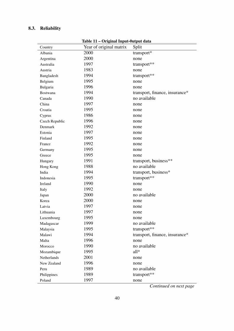
8.3. Reliability
Table 11 – Original Input-0utput dataCountry Year of original matrix SplitAlbania 2000 transport*Argentina 2000 noneAustralia 1997 transport**Austria 1983 noneBangladesh 1994 transport**Belgium 1995 noneBulgaria 1996 noneBostwana 1994 transport, finance, insurance*Canada 1990 no availableChina 1997 noneCroatia 1995 noneCyprus 1986 noneCzech Republic 1996 noneDenmark 1992 noneEstonia 1997 noneFinland 1995 noneFrance 1992 noneGermany 1995 noneGreece 1995 noneHungary 1991 transport, business**Hong Kong 1988 no availableIndia 1994 transport, business*Indonesia 1995 transport**Ireland 1990 noneItaly 1992 noneJapan 2000 no availableKorea 2000 noneLatvia 1997 noneLithuania 1997 noneLuxembourg 1995 noneMadagascar 1999 no availableMalaysia 1995 transport**Malawi 1994 transport, finance, insurance*Malta 1996 noneMorocco 1990 no availableMozambique 1995 all*Netherlands 2001 noneNew Zealand 1996 nonePeru 1989 no availablePhilippines 1989 transport**Poland 1997 none
Continued on next page
40
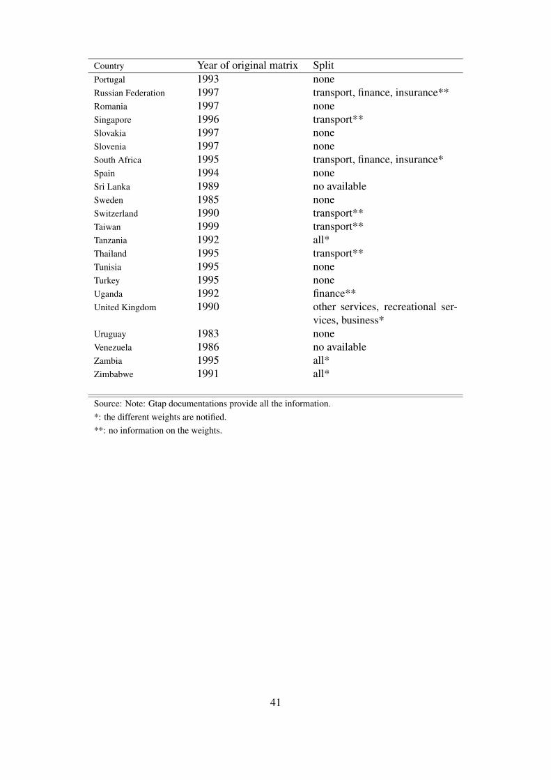
Country Year of original matrix SplitPortugal 1993 noneRussian Federation 1997 transport, finance, insurance**Romania 1997 noneSingapore 1996 transport**Slovakia 1997 noneSlovenia 1997 noneSouth Africa 1995 transport, finance, insurance*Spain 1994 noneSri Lanka 1989 no availableSweden 1985 noneSwitzerland 1990 transport**Taiwan 1999 transport**Tanzania 1992 all*Thailand 1995 transport**Tunisia 1995 noneTurkey 1995 noneUganda 1992 finance**United Kingdom 1990 other services, recreational ser-
vices, business*Uruguay 1983 noneVenezuela 1986 no availableZambia 1995 all*Zimbabwe 1991 all*
Source: Note: Gtap documentations provide all the information.*: the different weights are notified.**: no information on the weights.
41
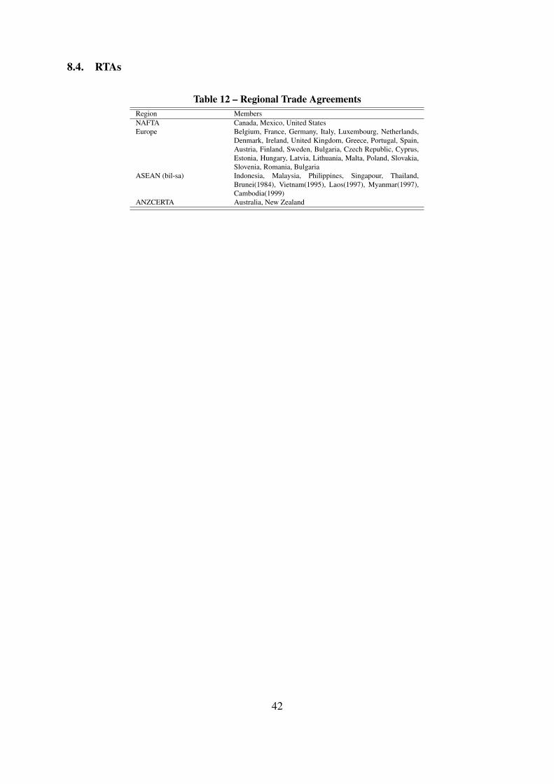
8.4. RTAs
Table 12 – Regional Trade AgreementsRegion MembersNAFTA Canada, Mexico, United StatesEurope Belgium, France, Germany, Italy, Luxembourg, Netherlands,
Denmark, Ireland, United Kingdom, Greece, Portugal, Spain,Austria, Finland, Sweden, Bulgaria, Czech Republic, Cyprus,Estonia, Hungary, Latvia, Lithuania, Malta, Poland, Slovakia,Slovenia, Romania, Bulgaria
ASEAN (bil-sa) Indonesia, Malaysia, Philippines, Singapour, Thailand,Brunei(1984), Vietnam(1995), Laos(1997), Myanmar(1997),Cambodia(1999)
ANZCERTA Australia, New Zealand
42

LIST OF WORKING PAPERS RELEASED BY CEPII
43