Estimation with Many Instrumental Variables∗

Christian HansenGraduate School of BusinessUniversity of Chicago

Jerry HausmanDepartment of Economics

M.I.T.

Whitney NeweyDepartment of Economics

M.I.T.

December 2004Revised, August 2006

Abstract

Using many valid instrumental variables has the potential to improve efficiencybut makes the usual inference procedures inaccurate. We give corrected standarderrors, an extension of Bekker (1994) to nonnormal disturbances, that adjust formany instruments. We find that this adjustment is useful in empirical work, simula-tions, and in the asymptotic theory. Use of the corrected standard errors in t-ratiosleads to an asymptotic approximation order that is the same when the number ofinstrumental variables grows as when the number of instruments is fixed. We alsogive a version of the Kleibergen (2002) weak instrument statistic that is robust tomany instruments.

JEL Classification: C13, C21, C31Keywords: Weak Instruments, Many Instruments, Standard Errors, Inference

Corresponding Author: Whitney Newey, E52-262D, MIT, Cambridge, MA 02139,wnewey@mit.edu

∗The NSF provided financial support for this paper under Grant No. 0136869. Helpful commentswere provided by A Chesher, T. Rothenberg, J. Stock, and participants in seminars at Berkeley, Bristol,Cal Tech, Harvard-MIT, Ohio State, Stanford, the University of Texas - Austin, UCL, and the Universityof Virginia.

1 Introduction

Empirical applications of instrumental variables estimation often give imprecise results.

Using many valid instrumental variables can improve precision. For example, as we show,

using all 180 instruments in the Angrist and Krueger (1991) schooling application gives

tighter correct confidence intervals than using 3 instruments. An important problem with

using many instrumental variables is that conventional asymptotic approximations may

provide poor approximations to the sampling distributions of the resulting estimators.

Two stage least squares (2SLS) is well known to have large biases when many instruments

are used. The limited information maximum likelihood (LIML henceforth) or Fuller

(1977, FULL henceforth) estimators correct this bias, but the usual standard errors are

too small.

We give corrected standard errors (CSE) that improve upon the usual ones, leading

to a better normal approximation to t-ratios under many instruments. The CSE are

an extension of those of Bekker (1994) that allow for non Gaussian disturbances. We

show that the normal approximation with FULL and CSE is asymptotically correct with

nonnormal disturbances under a variety of many instrument asymptotics, including the

many instrument sequence of Kunitomo (1980), Morimune (1983), and Bekker (1994)

and the many weak instruments sequence of Chao and Swanson (2002, 2003, 3004, 2005)

and Stock and Yogo (2004). We also find that there is no penalty for many instruments in

the rate of approximation for t-ratios when the CSE are used and an additional condition

is satisfied. That is, the rate of approximation is the same as with a fixed number of

instruments. In addition, we give a version of the Kleibergen (2002) test statistic that is

valid under many instruments, as well as under weak instruments.

We carry out a wide range of simulations to check the asymptotic approximations. We

find that FULL with the CSE give confidence intervals with actual coverage quite close to

nominal. We also show that LIML with the CSE has identical asymptotic properties to

FULL and performs quite well in our simulations, as in those of Hahn and Inoue (2002).

Our results also demonstrate that the concentration parameter (which can be estimated)

[1]

provides a better measure of accuracy for standard inference with FULL or LIML than

the F-statistic, R2, or other statistics previously considered in the literature.

In relation to previous work, the CSE, the rate of approximation results, and our many

instrument view of the Angrist and Krueger (1991) application appear to be novel. The

limiting distribution results build on previous work. For many instrument asymptotics

we generalize LIML results of Kunitomo (1980), Morimune (1983), Bekker (1994), and

Bekker and van der Ploeg (2005) to FULL, disturbances that are not Gaussian, and

general instruments. Our results also generalize recent results of Anderson, Kunitomo,

and Matsushita (2006) to many weak instruments, who had generalized results from

an earlier version of this paper by relaxing a conditional moment restriction. We also

combine and generalize results of Chao and Swanson (2002, 2003, 2005) and Stock and

Yogo (2004) by relaxing some kurtosis restrictions of Chao and Swanson (2003) and

allowing a wider variety of sequences of instruments and concentration parameter than

Stock and Yogo (2004). Our theoretical results make use of some inequalities in Chao

and Swanson (2004).

Hahn and Hausman (2002) give a test for weak instruments and Hahn, Hausman,

and Kuersteiner (2004) show that FULL performs well under weak instruments. Recently

Andrews and Stock (2006) derive asymptotic power envelopes for tests under several cases

of many weak instrument asymptotics with Gaussian disturbances. We consider cases

where the square root of the number of instruments grows slower than the concentration

parameter. There it turns out that Wald tests using the CSE attain the power envelope.

We also consider a case where the number of instruments grows as fast as the sample

size, which is not covered by Andrews and Stock (2006).

The remainder of the paper is organized as follows. In the next section, we briefly

present the model and estimators that we will consider. We reexamine the Angrist

and Krueger (1991) study of the returns to schooling in Section 3 and give a variety

of simulation results in Section 4. Section 5 contains asymptotic results and Section 6

concludes.

[2]

2 Models and Estimators

The model we consider is given by

yT×1

= XT×G

δ0G×1

+ uT×1

,

X = Υ+ V,

where T is the number of observations, G the number of right-hand side variables, Υ

is a matrix of observations on the reduced form, and V is the matrix of reduced form

disturbances. For the asymptotic approximations, the elements of Υ will be implicitly

allowed to depend on T , although we suppress dependence of Υ on T for notational

convenience. Estimation of δ0 will be based on a T × K matrix Z of instrumental

variable observations.

This model allows for Υ to be a linear combination of Z, i.e. Υ = Zπ for some K×G

matrix π. Furthermore, columns of X may be exogenous, with the corresponding column

of V being zero. The model also allows for Z to be functions meant to approximate the

reduced form. For example, let Υt and Zt denote the tth row (observation) for Υ and

Z respectively. We could have Υt = f0(wt) be an unknown function of a vector wt

of underlying instruments and Zt = (p1K(wt), ..., pKK(wt))0 for approximating functions

pkK(w), such as power series or splines. In this case linear combinations of Zt may

approximate the unknown reduced form, e.g. as in Donald and Newey (2001).

It is well known that variability of Υ relative to V is important for the properties of

instrumental variable estimators. For G = 1 this feature is well described by

μ2T =TXt=1

Υ2t/E[V

2t ].

This concentration parameter plays a central role in the theory of IV estimators. The

distribution of the estimators depends on μ2T , with the convergence rate being 1/μT and

the accuracy of the usual asymptotic approximation depending crucially on the size of

μ2T .

To describe the estimators, let P = Z(Z 0Z)−Z 0 where A− denotes any symmetric

generalized inverse of a symmetric matrix A, i.e. A− is symmetric and satisfies AA−A =

[3]

A. We consider estimators of the form

δ = (X 0PX − αX 0X)−1(X 0Py − αX 0y).

for some choice of α. This class includes all of the familiar k-class estimators except the

least squares estimator. Special cases of these estimators are two-stage least squares

(2SLS), where α = 0, and LIML, where α = α and α is the smallest eigenvalue of the

matrix (X 0X)−1X 0PX for X = [y,X]. FULL is also a member of this class of estimators,

where α = [α− (1− α)C/T ]/[1− (1− α)C/T ] for some constant C. FULL has moments

of all orders, is approximately mean unbiased for C = 1, and is second order admissible

for C ≥ 4 under standard large sample asymptotics.

For inference we consider an extension of the Bekker (1994) standard errors to nonnor-

mality and estimators other then LIML. Let u(δ) = y −Xδ, σ2u(δ) = u(δ)0u(δ)/(T −G),

α(δ) = u(δ)0Pu(δ)/u(δ)0u(δ), Υ = PX, X(δ) = X − u(δ)(u(δ)0X)/u(δ)0u(δ), V (δ) =

(I − P )X(δ), κT =PT

t=1 P2tt/K, τT = K/T,

H(δ) = X 0PX − α(δ)X 0X,

ΣB(δ) = σ2u(δ)(1− α(δ))2X(δ)0PX(δ) + α(δ)2X(δ)0(I − P )X(δ),

Σ(δ) = ΣB(δ) + A(δ) + A(δ)0 + B(δ), A(δ) =TXt=1

(Ptt − τT ) Υt[TXt=1

ut(δ)2Vt(δ)/T ]

0,

B(δ) = K(κT − τT )TXt=1

(ut(δ)2 − σ2u(δ))Vt(δ)Vt(δ)

0/[T (1− 2τT + κT τT )].

The asymptotic variance estimator is given by

Λ = H−1ΣH−1, H = H(δ), Σ = Σ(δ).

When δ is the LIML estimator, H−1ΣB(δ)H−1 is identical to the Bekker (1994) variance

estimator. The other terms in Λ account for third and fourth moment terms that are

present with some forms of nonnormality. In general Λ is a ”sandwich” formula, with H

being a Hessian term.

The variance estimator Λ can be quite different than the usual one σ2uH−1 even when

K is small relative to T. This occurs because H is close to the sum of squares of predicted

[4]

values for the reduced form regressions and ΣB(δ) depends on sums of squares of residuals.

When the reduced form R2 is small, the sum of squared residuals will tend to be quite

large relative to H, leading to ΣB(δ) being larger than H. In contrast, the adjustments

for nonnormality A(δ) and B(δ) will tend to be quite small when K is small relative

to T , which is typical in applications. Thus we expect that in applied work the Bekker

(1994) standard errors and CSE will often give very similar results.

As shown by Dufour (1997), if the parameter set is allowed to include values where

Υ = 0 then a correct confidence interval for a structural parameter must be unbounded

with probability one. Hence, confidence intervals formed using the CSE cannot be cor-

rect. Also, under the weak instrument sequence of Staiger and Stock (1997) the CSE

confidence intervals will not be correct, i.e. they are not robust to weak instruments.

These considerations motivate consideration of a statistic that is asymptotically correct

with weak or many instruments.

Such a statistic can be obtained by modifying the Lagrange multiplier statistic of

Kleibergen (2002) and Moreira (2001). For any δ let

LM(δ) = u(δ)0PX(δ)Σ(δ)−1X(δ)0Pu(δ).

This statistic differs from previous ones in using Σ(δ)−1 in the middle. Its validity

does not depend on correctly specifying the reduced form. The statistic LM(δ) will be

asymptotically distributed as χ2(G) when δ = δ0 under both many and weak instruments.

Confidence intervals for δ0 can be formed from LM(δ) by inverting it. Specifically, for

the 1−α quantile q of a χ2(G) distribution, an asymptotic 1−α confidence interval is δ :

LM(δ) ≤ q. As recently shown by Andrews and Stock (2006), the conditional likelihood

ratio test of Moreira (2003) is also correct with weak and many weak instruments, though

apparently not under many instruments, where K grows as fast as T . For brevity we

omit a description of this statistic and the associated asymptotic theory.

We suggest that the CSE are useful despite their lack of robustness to weak instru-

ments. Standard errors provide a simple measure of uncertainty associated with an esti-

mate. The confidence intervals based on LM(δ) are more difficult to compute. Also, as

[5]

we discuss below, the t-ratios for FULL based on the CSE provide a good approximation

over a wide range of empirically relevant cases. This observation might justify viewing

the parameter space as being bounded away from Υ = 0, thus overcoming the strict

Dufour (1997) critique. Or, one might simply view that our theoretical and simulation

results are relevant enough for applications to warrant using the CSE.

It does seem wise to check for weak instruments in practice. One could use the Hahn

and Hausman (2004) test. One could also compare a Wald test based on the CSE with

a test based on LM(δ). One could also develop versions of the Stock and Yogo (2004)

tests for weak instruments that are based on the CSE.

Because the concentration parameter is important for the properties of the estimators

it is useful to have an estimate of it for the common case with one endogenous right-hand

side variable. For G = 1 let σ2V = V 0V /(T −K). An estimator of μ2T is

μ2T = X 0X/σ2V −K = K(F − 1),

where F = (X 0X/K)/[V 0V /(T −K)] is the reduced form F-statistic. This estimator is

consistent in the sense that under many instrument asymptotics

μ2Tμ2T

p−→ 1.

In the general case with one endogenous right-hand side and other exogenous right-hand

side variables we take

μ2T = (K −G+ 1)(F − 1),

where F is the reduced form F-statistic for the variables in Z that are excluded from X.

3 Quarter of Birth and Returns to Schooling

A motivating empirical example is provided by the Angrist and Krueger (1991) study

of the returns to schooling using quarter of birth as an instrument. We consider data

drawn from the 1980 U. S. Census for males born in 1930-1939. The model includes

a constant and year and state dummies. We report results for 3 instruments and for

[6]

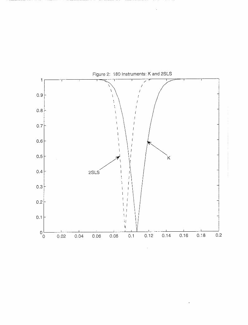
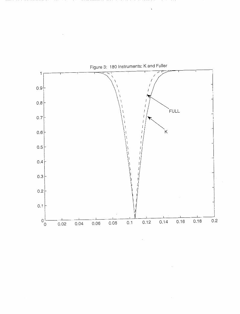
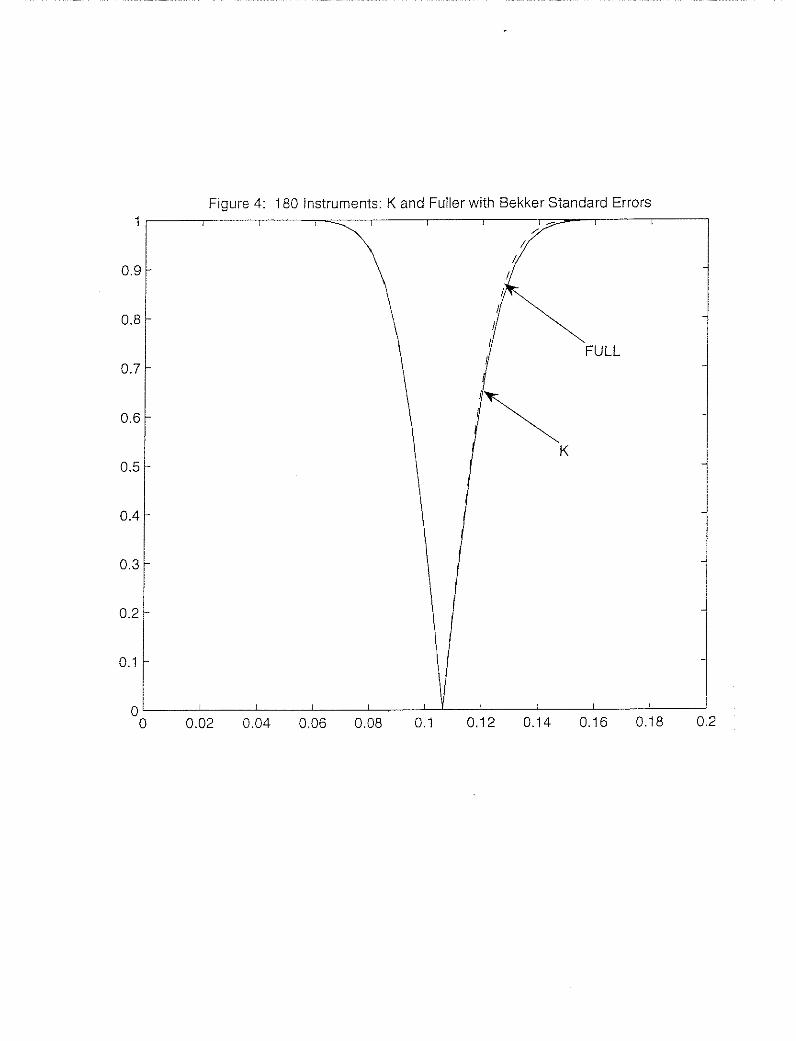
180 instruments. Figures 1-4 are graphs of confidence intervals at different significance

levels using several different methods. The confidence intervals we consider are based

on 2SLS with the usual (asymptotic) standard errors, FULL with the usual standard

errors, and FULL with the CSE. We take as a standard of comparison our version of the

Kleibergen (2002) confidence interval (denoted K in the graphs), which is robust to weak

instruments, many instruments, and many weak instruments.

Figure 1 shows that with three excluded instruments (two overidentifying restrictions),

2SLS and K intervals are very similar. The main difference seems to be a slight horizontal

shift. Since the K intervals are centered about the LIML estimator, this shift corresponds

to a slight difference in the LIML and 2SLS estimators. This difference is consistent with

2SLS having slightly higher bias than LIML. Figure 2 shows that with 180 excluded

instruments (179 overidentifying restrictions) the confidence intervals are quite different.

In particular, there is a much more pronounced shift in the 2SLS location, as well as

smaller dispersion. These results are consistent with a larger bias in 2SLS resulting from

many instruments.

Figure 3 compares the confidence interval for FULL based on the usual standard error

formula for 180 instruments with the K interval. Here we find that the K interval is wider

than the usual one. In Figure 4, we compare FULL with CSE to K, finding that the K

interval is nearly identical to the one based on the CSE.

Comparing Figures 1 and 4, we find that the CSE interval with 180 instruments is

substantially narrower than the intervals with 3 instruments. Thus, in this application

we find that using the larger number of instruments leads to more precise inference, as

long as FULL and the CSE are used. These graphs are consistent with direct calculations

of estimates and standard errors. The 2SLS estimator with 3 instruments is .1077 with

standard error .0195 and the FULL estimator with 180 instruments is .1063 with CSE

.0143. A precision gain is evident in the decrease in the CSE obtained with the larger

number of instruments. These results are also consistent with Donald and Newey’s (2001)

finding that using 180 instruments gives smaller estimated asymptotic mean square error

for LIML than using just 3. Furthermore, Cruz and Moreira (2005) also find that 180

[7]

instruments are informative when extra covariates are used.

We also find that the CSE and the standard errors of Bekker (1994) are nearly identical

in this application. Adding significant digits, with 3 instruments the CSE is .0201002

while the Bekker (1994) standard error is .0200981, and with 180 instruments the CSE

.0143316 and the Bekker (1994) standard error is .0143157. They are so close in this

application because even when there are 179 overidentifying restrictions, the number of

instruments is very small relative to the sample size.

These results are interesting because they occur in a widely cited application. However

they provide limited evidence of the accuracy of the CSE because they are only an

example. They result from one realization of the data, and so could have occurred by

chance. Real evidence is provided by a Monte Carlo study.

We based a study on the application to help make it empirically relevant. The design

had the same sample size as the application and instrument observations fixed at the sam-

ple values, e.g. as in Staiger and Stock’s (1997) design for dummy variable instruments.

The data was generated from a two equation triangular simultaneous equations system

with structural equation as in the empirical application and a reduced form consisting

of a regression of schooling on all of the instruments, including the covariates from the

structural equation. The structural parameters were set equal to their LIML estimated

values from the 3 instruments case. The disturbances were homoskedastic Gaussian with

(bivariate) variance matrix for each observation equal to the estimate from the applica-

tion. Because the design has parameters equal to estimates this Monte Carlo study could

be considered a parametric bootstrap.

We carried out two experiments, one with three excluded instruments and one with

179 excluded instruments. In each case the reduced form coefficients were set so that

the concentration parameter for the excluded instruments was equal to the unbiased

estimator from the application. With 3 overidentifying restrictions the concentration

parameter value was set equal to the value of the consistent estimator μ2T = 95.6 from

the data and with 179 overidentifying restrictions the value was set to μ2T = 257.

[8]

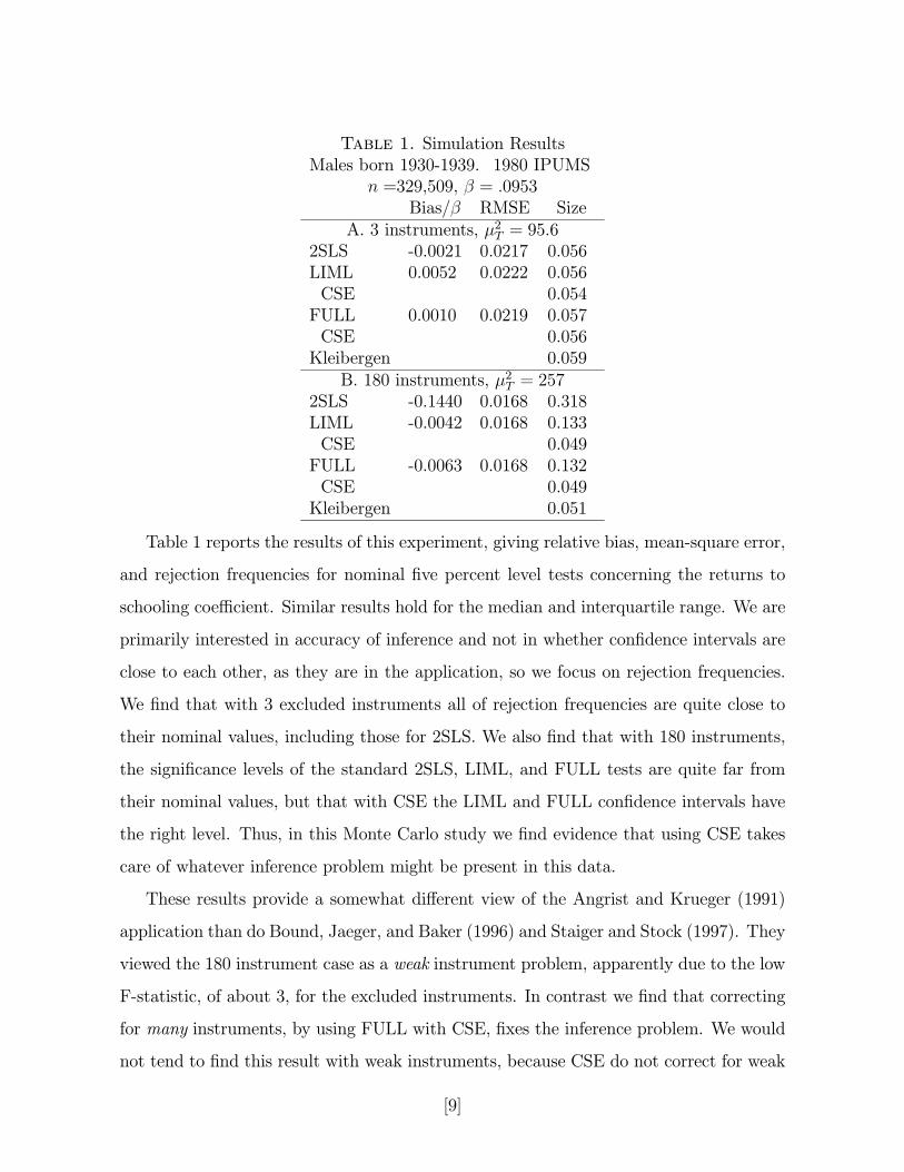
Table 1. Simulation ResultsMales born 1930-1939. 1980 IPUMS

n =329,509, β = .0953Bias/β RMSE Size

A. 3 instruments, μ2T = 95.62SLS -0.0021 0.0217 0.056LIML 0.0052 0.0222 0.056CSE 0.054FULL 0.0010 0.0219 0.057CSE 0.056Kleibergen 0.059

B. 180 instruments, μ2T = 2572SLS -0.1440 0.0168 0.318LIML -0.0042 0.0168 0.133CSE 0.049FULL -0.0063 0.0168 0.132CSE 0.049Kleibergen 0.051

Table 1 reports the results of this experiment, giving relative bias, mean-square error,

and rejection frequencies for nominal five percent level tests concerning the returns to

schooling coefficient. Similar results hold for the median and interquartile range. We are

primarily interested in accuracy of inference and not in whether confidence intervals are

close to each other, as they are in the application, so we focus on rejection frequencies.

We find that with 3 excluded instruments all of rejection frequencies are quite close to

their nominal values, including those for 2SLS. We also find that with 180 instruments,

the significance levels of the standard 2SLS, LIML, and FULL tests are quite far from

their nominal values, but that with CSE the LIML and FULL confidence intervals have

the right level. Thus, in this Monte Carlo study we find evidence that using CSE takes

care of whatever inference problem might be present in this data.

These results provide a somewhat different view of the Angrist and Krueger (1991)

application than do Bound, Jaeger, and Baker (1996) and Staiger and Stock (1997). They

viewed the 180 instrument case as a weak instrument problem, apparently due to the low

F-statistic, of about 3, for the excluded instruments. In contrast we find that correcting

for many instruments, by using FULL with CSE, fixes the inference problem. We would

not tend to find this result with weak instruments, because CSE do not correct for weak

[9]

instruments as illustrated in the simulation results below. These results are reconciled by

noting that a low F-statistic does not mean that FULL with CSE is a poor approximation.

As we will see, a better criterion for LIML or FULL is the concentration parameter.

In the Angrist and Krueger (1991) application we find estimates of the concentration

parameter that are quite large. With 3 excluded instruments μ2T = 95.6 and with 179

excluded instruments μ2T = 257. Both of these are well within the range where we find

good performance of FULL and LIML with CSE in the simulations reported below.

4 Simulations

To gain a broader view of the behavior of LIML and FULL with the CSE we consider the

weak instrument limit of the FULL and LIML estimators and t-ratios with CSE under

the Staiger and Stock (1997) asymptotics. This limit is obtained by letting the sample

size go to infinity while holding the concentration parameter fixed. The limits of CSE

and the Bekker (1994) standard errors coincide under this sequence because K/T −→ 0.

As shown in Staiger and Stock (1997), these limits provides excellent approximations to

small sample distributions. Furthermore, it seems very appropriate for microeconometric

settings, where the sample size is often quite large relative to the concentration parameter.

Tables 2-5 give results for the median, interquartile range, and rejection frequencies

for nominal 5 percent level tests based on the CSE and the usual asymptotic standard

error for FULL and LIML, for a range of numbers of instruments K; concentration pa-

rameters μ2T ; and values of the correlation coefficient ρ between ut and Vt. These three

parameters completely determine the weak instrument limiting distribution of t-ratios.

Tables 2-5 give results for ρ = 0, ρ = 0.2, ρ = 0.5, and ρ = 0.8 respectively. Each table

contains results for several different numbers of instruments and values of the concentra-

tion parameter.

Looking across the tables, there are a number of striking results. We find that LIML

is nearly median unbiased for small values of the concentration parameter in all cases.

This bias does increase somewhat in ρ and K, but even in the most extreme case we

[10]

consider, with ρ = .8 and K = 32, the bias is virtually eliminated with a μ2 of 16. Also,

the bias is small when μ2 is 8 in almost every case. When we look at FULL, we see that

it is more biased than LIML but that it is considerably less dispersed. The differences

in dispersion are especially pronounced for low values of the concentration parameter,

though FULL is less dispersed than LIML in all cases.

The results for rejection frequencies are somewhat less clear cut than the results for

size and dispersion. In particular, the rejection frequencies tend to depend much more

heavily on the value of K and ρ than do the results for median bias or dispersion. For

LIML, the rejection frequencies when the CSE are used are quite similar to the rejection

frequencies when the usual asymptotic variance is used for small values of K, but the

CSE perform much better for moderate and large K, indicating that using the CSE with

LIML will generally be preferable. FULL with CSE performs better in some cases and

worse in others than FULL with the conventional standard errors when K is small but

clearly dominates for K large. The results also show that for small values of ρ, the

rejection frequencies for LIML and FULL tend to be smaller than the nominal value,

while the frequencies tend to be larger than the nominal value for large values of ρ.

An interesting and useful result is that both LIML and FULL with the CSE perform

reasonably well for all values of K and ρ in cases where the concentration parameter is

32 or higher. In these cases, the rejection frequency for LIML varies between .035 and

.06, and the rejection frequency for FULL varies between .035 and .070. These results

suggest that the use of LIML or FULL with the CSE and the asymptotically normal

approximation should be adequate in situations where the concentration parameter is

around 32 or greater, even though in many of these cases the F-statistic takes on small

values.

These results are also consistent with recent Monte Carlo work of Davidson and

MacKinnon (2004). From careful examination of their graphs it appears that with few

instruments the bias of LIML is very small once the concentration parameter exceeds 10,

and that the variance of LIML is quite small once the concentration parameter exceeds

20.

[11]

To see which cases might be empirically relevant we summarize values of K and esti-

mates of μ2 and ρ from some empirical studies. We considered all microeconomic studies

that contain sufficient information to allow estimation of these quantities found in the

March 1999 to March 2004 American Economic Review, the February 1999 to June 2004

Journal of Political Economy, and the February 1999 to February 2004 Quarterly Journal

of Economics. We found that 50 percent of the papers had at least one overidentifying

restriction, 25 percent had at least three, and 10 percent had 7 or more. As we have seen,

the CSE can provide a substantial improvement even with small numbers of overidenti-

fying restrictions, so there appears to be wide scope for applying these results. Table 7

summarizes estimates of μ2 and ρ from these studies.

Table 7. Five years of AER, JPE, QJE.Num Papers Median Q10 Q25 Q75 Q90

μ2 28 23.6 8.95 12.7 105 588ρ 22 .279 .022 .0735 .466 .555

It is interesting to note that nearly all of the studies had values of ρ that were

quite low, so that the ρ = .8 case considered above is not very relevant for practice.

Also, the concentration parameters were mostly in the range where the many instrument

asymptotics with CSE should work well.

5 Many Instrument Asymptotics

Theoretical justification of the CSE is provided by asymptotic theory where the number

of instruments grows with the sample size and using the CSE in t-ratios leads to a better

asymptotic approximation (by the standard normal) than do the usual standard errors.

This theory is consistent with the empirical and Monte Carlo results where the CSE

improve accuracy of the Gaussian approximation.

Some regularity conditions are important for the results. Let Z 0t, ut, V0t , and Υ

0t denote

the tth row of Z, u, V, and Υ respectively. Here we will consider the case where Z is

constant, leaving the treatment of random Z to future research.

[12]

Assumption 1: Z includes among its columns a vector of ones, rank(Z) = K,PTt=1(1− ptt)

2/T ≥ C > 0.

The restriction that rank(Z) = K is a normalization that requires excluding redun-

dant columns from Z. It can be verified in particular cases. For instance, whenwt is a con-

tinuously distributed scalar, Zt = pK(wt), and pkK(w) = wk−1 it can be shown that Z 0Z is

nonsingular with probability one forK < T .1 The conditionPT

t=1(1−ptt)2/T ≥ C implies

thatK/T ≤ 1−C, because ptt ≤ 1 impliesPT

t=1(1−ptt)2/T ≤PT

t=1(1−ptt)/T = 1−K/T.

Assumption 2: There is a G × G matrix ST = ST diag (μ1T , ..., μGT ) and zt such

that Υt = STzt/√T , ST is bounded and the smallest eigenvalue of ST S

0T is bounded away

from zero, for each j either μjT =√T or μjT/

√T −→ 0, μT = min

1≤j≤GμjT −→ ∞, and

√K/μ2T −→ 0. Also,

PTt=1 kztk

4 /T 2 −→ 0, andPT

t=1 ztz0t/T is uniformly nonsingular.

Allowing for K to grow and for μT to grow slower than√T models having many

instruments without strong identification. Assumption 2 will imply that, when K grows

no faster that μ2T , the convergence rate of δ will be no slower than 1/μT . When K grows

faster than μ2T the convergence rate of δ will be no slower than√K/μ2T . This condition

allows for some components of δ to be weakly identified and other components (like the

constant) to be strongly identified.

Assumption 3: (u1, V1), ..., (uT , VT ) are independent with E[ut] = 0, E[Vt] = 0,

E[u8t ] and E[kVtk8] are bounded in t, V ar((ut, V 0t )0) = diag(Ω∗, 0), Ω∗ is nonsingular, and

for all j ∈ 1, ..., G such that Vtj = 0 and the corresponding submatrix ST22 of ST it is

the case that μjT =√T and ST22 is uniformly nonsingular.

This hypothesis includes moment existence and homoskedasticity assumptions. The

consistency of the CSE depends on homoskedasticity, as does consistency of the LIML

estimator itself with many instruments; see Bekker and van der Ploeg (2005), Chao and

Swanson (2004), and Hausman, Newey, and Woutersen (2006).

1The observations w1, ..., wT are distinct with probability one and therefore, by K < T, cannot allbe roots of a Kth degree polynomial. It follows that for any nonzero a there must be some t witha0Zt = a0pK(wt) 6= 0, implying a0Z 0Za > 0.

[13]

Assumption 4: There is πKT such that ∆2T =

PTt=1 kzt − πKTZtk2 /T −→ 0.

This condition allows an unknown reduced form that is approximated by a linear

combination of the instrumental variables. An important example is a model with

Xt =

Ãπ11Z1t + μTf0(wt)/

√T

Z1t

!+

ÃV1t0

!, Zt =

ÃZ1t

pK(wt)

!,

where Z1t is a G2 × 1 vector of included exogenous variables, f0(w) is a G − G2 di-

mensional vector function of a fixed dimensional vector of exogenous variables w and

pK(w)def= (p1K(w), ..., pK−G2,K(w))

0. The other variables in Xt other than Z1t are en-

dogenous with reduced form π11Z1t+μTf0(wt)/√T . The function f0(w) may be a linear

combination of a subvector of pK(w), in which case ∆T = 0 in Assumption 4 or it may

be an unknown function that can be approximated by a linear combination of pK(w).

For μT =√T this example is like the model in Donald and Newey (2001) where Zt

includes approximating functions for the optimal (asymptotic variance minimizing) in-

struments Υt, but the number of instruments can grow as fast as the sample size. When

μ2T/T −→ 0, it is a modified version where the model is more weakly identified.

To see precise conditions under which the assumptions are satisfied, let

zt =

Ãf0(wt)Z1t

!, ST = STdiag

³μT , ..., μT ,

√T , ...,

√T´, ST =

ÃI π110 I

!.

By construction we have Υt = STzt/T. Assumption 2 imposes the requirements that

TXt=1

kztk4 /T 2 −→ 0,TXt=1

ztz0t/T is uniformly nonsingular.

The other requirements of Assumption 2 are satsified by construction. Turning to As-

sumption 3, we require that V ar(ut, V01t) is nonsingular. Since the submatrix of ST

corresponding to Vtj = 0 is the same as the submatrix corresponding to the included

exogenous variables Z1t, we have ST22 = I is uniformly nonsingular. For Assumption 4,

let πKT = [π0KT , [IG2 , 0]

0]0. Then Assumption 4 will be satisfied if for each T there exists

πKT with

∆2T =

TXt=1

kzt − π0KTZtk2/T =TXt=1

kf0(wt)− π0KTZtk2/T −→ 0.

[14]

The following is a consistency result.

Theorem 1: If Assumptions 1-4 are satisfied and α = K/T +op(μ2T/T ) or δ is LIML

or FULL then μ−1T S0T (δ − δ0)p−→ 0 and δ

p−→ δ0.

This result is more general than Chao and Swanson (2005) in allowing for strongly

identified covariates but is similar to Chao and Swanson (2003). See Chao and Swanson

(2005) for an interpretation of the condition on α. This result gives convergence rates

for linear combinations of δ. For instance, in the linear model example set up above, it

implies that δ1 is consistent and that π011δ1 + δ2 = op(μT/

√T ).

Before stating the asymptotic normality results we describe their form. Let σ2u =

E[u2t ], σ2V u = E[Vtut], γ = σV u/σ

2u, V = V −uγ0, having tth row V 0

t . and let Ω = E[VtV0t ].

There will be two cases depending on the speed of growth of K relative to μ2T .

Assumption 5: Either I) K/μ2T is bounded or II) K/μ2T −→∞.

To state a limiting distribution result it is helpful to also assume that certain objects

converge. When considering the behavior of t-ratios we will drop this condition.

Assumption 6: H = limT−→∞

(1 − τT )z0z/T , τ = lim

T−→∞τT , κ = lim

T−→∞κT , A =

E[u2t Vt] limT−→∞

PTt=1 z

0t(ptt − K

T)/√KT exist and in case I)

√KS−1T −→ S0 or in case

II) μTS−1T −→ S0.

Below we will give results for t-ratios that do not require this condition. Let B =

(κ− τ)E[(u2t − σ2u)VtV0t ]. Then in case I) we will have

S0T (δ − δ0)d−→ N(0,ΛI), S

0T ΛST

p−→ ΛI ,ΛI = H−1ΣIH−1, (5.1)

ΣI = (1− τ)σ2uH + S0ΩS00+ (1− τ)(S0A+A0S00) + S0BS

00.

In case II we will have

(μT/√K)S0T (δ − δ0)

d−→ N(0,ΛII), (μ2T/K)S

0T ΛST

p−→ ΛII ,ΛII = H−1ΣIIH−1,(5.2)

[15]

ΣII = S0[(1− τ)σ2uΩ+B]S00.

The asymptotic variance expressions allow for the many instrument sequence of Ku-

nitomo (1980), Morimune (1983), and Bekker (1994) and the many weak instrument

sequence of Chao and Swanson (2003, 2005). When K and μ2T grow as fast as T the

variance formula generalizes that of Anderson et. al. (2006) to include the coefficients of

included exogenous variables, which had previously generalized Hansen et. al. (2004) to

allow for E[ut|Vt] 6= 0 and E[u2t |Vt] 6= σ2u. This formula also extends that of Bekker and

van der Ploeg (1995) to general instruments. The formula also generalizes Anderson et.

al. (2006) to allow for μ2T and K to grow slower than T . Then τ = κ = 0, A = 0, and

B = 0 giving a formula which generalizes Stock and Yogo (1994) to allow for included

exogenous variables and to allow for K to grow faster than μ2T , similarly to Chao and

Swanson (2004). When K does grow faster than μ2T the asymptotic variance of δ may

be singular. This occurs because the many instruments adjustment term is singular with

included exogenous variables and it dominates the nonsingular matrix H when K grows

that fast.

Theorem 2: If Assumptions 1-6 are satisfied, α = α + Op(1/T ) or δ is LIML or

FULL, then in case I) equation (5.1) is satisfied and in case II) equation (5.2) is satisfied.

Also, in each case if Σ is nonsingular then LM(δ0)d−→ χ2(G).

Recently Andrews and Stock (2006) have derived the power envelope for a test of

H0 : δ0 = δ under many weak instruments with Gaussian disturbances and scalar δ.

Under the restriction√K/μ2T −→ 0 that we impose the Wald test with the CSE is

optimal, attaining this power envelope. This result follows from optimality of the LM

statistic of Kleibergen (2002), as shown by Andrews and Stock (2006), and asymptotic

equivalence of the Wald and LM statistic under local alternatives. For brevity we omit

the demonstration of asymptotic equivalence of the Wald and LM statistics.

To give results for t-ratios and to understand better the performance of the CSE we

now turn to approximation results. We will give order of approximation results for two

[16]

t-ratios involving linear combinations of coefficients, one with the CSE and another with

the usual formula, and compare results.

We first give stochastic expansions around a normalized sum with remainder rate. To

describe these results we need some additional notation. Define

H = X 0PX − αX 0X, W = [(1− τT )Υ+ PZV − τT V ]S−10T ,HT = (1− τT )z

0z/T,

AT =

ÃTXt=1

(ptt − τT )zt/√T

!E[u2t V

0t ]S

−10T , BT = (κT − τT )E[(u

2t − σ2u)VtV

0t ],

ΣT = σ2u(1− τT )(HT +KS−1T ΩS−10T ) + (1− τT )(AT +A0T ) +KS−1T BTS−10T ,

ΛT = H−1T ΣTH

−1T .

We will consider t-ratios for a linear combination c0δ of the IV estimator, where c are the

linear combination coefficients, satisfying the following condition:

Assumption 7: There is μcT such that μcT c0S−10T is bounded and in case I) (μcT )

2c0S−10T ΛTS−1T c

and (μcT )2c0S−10T H−1

T S−1T c are bounded away from zero and in case II) (μcT )2c0S−10T ΛTS

−1T cμ2T/K

is bounded away from zero.

Let μT = μT in case I and μT = μ2T/√K in case II.

Theorem 3: Suppose that Assumptions 1 - 5 and 7 are satisfied and α = α+Op(1/T )

or δ is LIML or FULL. Then, for εT = ∆T + 1/μT in case I) and case II),

c0(δ − δ0)qc0Λc

d−→ N(0, 1),c0(δ − δ0)q

c0Λc=

c0S−10T H−1T W 0uq

c0S−10T ΛTS−1T c

+Op(εT ).

Also, in case II), Pr(¯c0(δ − δ0)/

qσ2uc

0H−1c¯≥ C) −→ 1 for all C while in case I),

c0(δ − δ0)qσ2uc

0H−1c=

c0S−10T H−1T W 0uq

σ2uc0S−10T H−1

T S−1T c+Op(εT ).

Here we find that the t-ratio based on the linear combination c0δ is equal to a sum

of independent random variables, plus a remainder term that is of order 1/μT +∆T . It

is interesting to note that in case I the rate of approximation is 1/μT + ∆T and 1/μT

is the rate of approximation that would hold for fixed K. For example, when μ2T = T

[17]

and ∆T = 0, the rate of approximation is the usual parametric rate 1/√T . Thus, even

when K grows as fast as T , the remainder terms in Theorem 3 can have the parametric

1/√T rate. This occurs because the specification ofW accounts for the presence of many

instrumental variables.

The reason that the t-ratio with the usual standard errors is unbounded whenK/μ2T −→

∞ is that the usual variance formula goes to zero relative to the full variance. When

K grows that fast the term that adjusts for many instruments asymptotically dominates

the usual variance formula.

To obtain approximation rates for the distribution of the normalized sums in the

conclusion of Theorem 3, we impose the following restriction on the joint distribution of

ut and Vt.

Assumption 8: E[ut|Vt] = 0, E[u2t |Vt] = σ2u, E[|ut|4|Vt] is bounded, andPT

t=1 kztk3 /T 3/2 =

O(1/μT ).

The vector Vt consists of residuals from the population regression of Vt on ut and so

satisfies E[Vtut] = 0 by construction. Under joint normality of (ut, Vt), ut and Vt are

independent, so the first two conditions automatically hold. In general, these two condi-

tions weaken the joint normality restriction to first and second moment independence of

ut from Vt. For example, if Vt = γut + Vt for any Vt that is statistically independent of

ut then Assumption 4 would be satisfied. The asymptotic variance of the estimators are

simpler under these conditions. This condition implies that E[u2t Vt] = E[E[u2t |Vt]Vt] = 0

and E[u2t VtV0t ] = E[E[u2t |Vt]VtV 0

t ] = σ2uE[VtV0t ], so that AT = 0 and BT = 0.

Theorem 4: If Assumptions 1-5, 7 and 8 are satisfied then for case I

Pr(c0S−10T H−1

T W 0uqc0S−10T ΛTS

−1T c

≤ q) = Φ(q) +O(1/μT ),

Pr(c0S−10T H−1

T W 0uqσ2uc

0S−10T H−1T S−1T c

≤ q) = Φ(q) +O(1/μT +K/μ2T ).

When the variance ΛT that adjusts for the presence of many instruments appears in

the denominator the approximation is the fixed K rate 1/μT . In contrast, in case I when

[18]

the usual variance formula σ2uH−1T appears in the denominator, the rate of approximation

has an additional K/μ2T term. This term will go to zero slower than 1/μT when K grows

faster than μT . When K grows as fast as μ2T the remainder term does not even go to

zero, which corresponds to the usual standard errors being inconsistent.

We interpret this result as showing a clear advantage for the CSE with many in-

strumental variables. The condition for the usual standard errors to have as good an

approximation rate as the CSE, that K grows slower than μT , may seem not very onerous

when μT =√T . However, when μT grows slower than

√T this condition would put severe

limits on the number of instrumental variables. Thus, if we think of μT growing slowly

as representing a weakly identified model we should expect to find an improvement from

using the CSE even with small numbers of instrumental variables. This interpretation is

consistent with our empirical and Monte Carlo results.

It would be nice to combine Theorems 3 and 4 to obtain a result on the rate of

distributional approximation for the t-ratio. It is well known that this will hold with

additional tail conditions on the remainder in the stochastic expansions of Theorem 3;

see Rothenberg (1984). To do this is beyond the scope of this paper.

We can also show that our modified version of the Kleibergen (2002) statistic is valid

under weak instruments.

Theorem 5: If Assumptions 1 - 3 are satisfied, for each j either μjT = 1 or μjT =√T , and S−1T −→ S0, Z

0Z/T −→M, nonsingular, and Z 0z/T −→ R , then LM(δ0)d−→

χ2(G).

6 Conclusion

In this paper, we have given standard errors that correct for many instruments when

disturbances are not Gaussian. We have also shown that the LIML and Fuller (1977)

estimators with Bekker (1994) standard errors provide improved inference relative to the

usual asymptotic approximation in instrumental variable settings across a wide range

of applications. The Angrist and Krueger (1991) study provides an example where the

[19]

CSE with 180 instruments is substantially smaller than the CSE with 3 instruments and

confidence intervals closely match those of Kleibergen (2002). Through simulations, we

confirm that using the CSE leads to more accurate approximations in many cases. We

also provide theoretical results that show the validity of the CSE under many instruments

and under many weak instruments without imposing normality. The theoretical results

also show that the use of the CSE improves the approximation rate relative to when the

usual standard errors are used. Overall, the results support the use of the CSE across a

wide variety of applications.

7 Appendix: Proofs of Theorems.

Throughout, let C denote a generic positive constant that may be different in different

uses and let M, CS, and T denote the conditional Markov inequality, the Cauchy-Schwartz

inequality, and the Triangle inequality respectively. Also, for notational convenience, we

drop the T subscript on μT throughout.

Lemma A1: If (ui, vi, zi) are independent with E[ui|zi] = E[vi|zi] = 0, E[u4i |zi] ≤ C,

E[v4i |zi] ≤ C, zi is K × 1, then for Z = [z1, ..., zT ] and P = Z(Z 0Z)−Z 0,

V ar(u0Pv|Z) ≤ CK,u0Pv −E[u0Pv|Z] = Op(√K).

Proof: Let σuvi = E[uivi|zi], μjui = E[(ui)j|zi], μjvi = E[(vi)

j|zi]. By independent observa-

tions, E[uv0|Z] = diag(σuv1, ..., σuvT ) = Γ. Then E[u0Pv|Z] = tr(PE[vu0|Z]) = tr(PZΓ).

Also, for pij = Pij,

E[(u0Pv)2|Z] (7.3)

=TX

i,j,k, =1

pijpk E[uivjukv |Z] =TXi=1

p2iiE[u2i v2i |zi] +

TXi6=j=1

(piipjj + p2ij)σuviσuvj + p2ijμ2uiμ

2vj

=TXi=1

p2iiE[u2i v2i |zi]− 2σ2uvi − μ2uiμ2vi+ tr(PZΓ)

2 +TX

i,j=1

p2ij(σuviσuvj + μ2uiμ2vj)

≤ CTXi=1

p2ii + CTX

i,j=1

p2ij + tr(PΓ)2 ≤ 2CTX

i,j=1

p2ij + tr(PZΓ)2

[20]

We havePT

j=1 p2ij = pii, so that by equation (7.3),

E[(u0Pv − E[u0Pv|Z])2|Z] ≤ CTX

i,j=1

p2ij ≤ CK.

The second conclusion follows by M. Q.E.D.

Lemma A2: If i) P is a constant idempotent matrix with rank(P ) = K; ii) (W1T , V1, u1),

..., (W1T , VT , uT ) are independent and DT =PT

t=1E[WtTW0tT ] is bounded; iii) (V

0t , ut)

has bounded fourth moments, E[Vt] = 0, E[ut] = 0, and E[(V 0t , ut)

0(V 0t , ut)] is constant;

iv)PT

t=1E[kWtTk4] −→ 0; v) K → ∞;then for Σdef= E[VtV

0t ]E[u

2t ] + E[Vtut]E[utV

0t ],

κT =PT

t=1 p2tt/K, and any sequence of bounded vectors c1T , c2T such that VT = c01TDT c1T+

(1− κT )c02T Σc2T is bounded away from zero it follows that

YT = V−1/2T (

TXt=1

c01TWtT + c02TXs 6=t

Vspstut/√K)

d−→ N (0, 1) .

Proof: Without changing notation let c1T = c1T/V−1/2T and c2T = c2T/V

−1/2T , and note

that these are bounded in T by VT bounded away from zero. Let wtT = c01TWtT and

vt = c02TVt, where we suppress the T subscript on vt for convenience. Then we have

YT = w1T +TXt=2

ytT , ytT = wtT +Xs<t

(vspstut + vtpstut)/√K.

Also, by E[kW1Tk4] ≤PT

t=1E[kWtTk4] −→ 0, so that E[w21T ] −→ 0 and hence

YT =TXt=2

ytT + op(1).

Note that ytT is martingale difference, so that we can apply a martingale central limit

theorem. It follows by P idempotent thatPT

s=1 p2st = ptt and

PTt=1 ptt = K. Then, for

DT =PT

t=1E[WtTW0tT ],

s2T = E

⎡⎣Ã TXt=2

ytT

!2⎤⎦ = TXt=1

E[w2tT ] +E

⎡⎢⎣⎛⎝Xs6=t

vspstut

⎞⎠2⎤⎥⎦ /K

= c01TDT c1T −E[w21T ] +Xs6=t

Xq 6=r

pstpqrE[vsutvqur]/q2n

= c01TDT c1T +nE[v2t ]E[u

2t ] + (E[vtut])

2o(1− κT ) + o(1)

= c01TDT c1T + c02T (1− κT )Σc2T + o(1) −→ 1.

[21]

Note that s2T is bounded and bounded away from zero. Also

TXt=2

E[y4tT ] ≤ CTXt=2

E[kWtTk4] + CTXt=2

E

⎡⎢⎣⎛⎝Xj<t

vtptjuj + vjptjut⎞⎠4⎤⎥⎦ /K2

By condition iv),PT

t=2E[kWtTk4] −→ 0. Also, by |pst| ≤ 1 andPT

j=1 p2ts = ptt,

TXt=2

E

⎡⎢⎣⎛⎝Xj<t

vtptjuj

⎞⎠4⎤⎥⎦ /K2 =

1

K2

TXt=2

Xj,k, ,m<t

ptjptkpt ptmE[v4t ujuku um]

=1

K2

TXt=2

Xj,k, ,m<t

E[v4t ]ptjptkpt ptmE[ujuku um] ≤C

K2

TXt=2

⎛⎝Xj<t

p4tj +Xj,k<t

p2tjp2tk

⎞⎠≤ C

K2

⎛⎝ TXt=1

TXj=1

p2tj +TXt=1

⎛⎝ TXj=1

p2tj

⎞⎠Ã TXk=1

p2tk

!⎞⎠ = C

K2

ÃTXt=1

ptt +TXt=1

p2tt

!≤ C

K−→ 0.

ThereforePT

t=2E[y4tT ] −→ 0, so the Lindbergh condition is satisfied. To apply the

martingale central limit theorem it now suffices to show that for Zt = (WtT , Vt, ut),

TXt=2

E[y2tT | Z1, ..., Zt−1]− s2Tp−→ 0 (7.4)

.Note first that by independence of W1T , ...,WTT ,

TXt=2

³E[w2tT | Z1, ..., Zt−1]− E[w2tT ]

´= 0.

Also

E

⎡⎣wtT

Xj<t

(vtptjuj + vjptjut)

⎤⎦ = 0and

E

⎡⎣wtT

Xj<t

(vtptjuj + vjptjut)/√K | Z1, ..., Zt−1

⎤⎦= E[wtTvt]

Xj<t

ptjuj/√K +E[wtTut]

Xj<t

ptjvj/√K.‘

Let δt = E[wtTvt] and consider the first term δtP

j<t ptjuj/√K. Let P be the up-

per triangular matrix with Ptj = Ptj for j > t and Ptj = 0, j ≤ t, and let δ =

(δ1, ..., δT ). ThenPT

t=2

Pj<t δtptjuj/

√K = δ0P 0u/

√K. By CS δ0δ =

PTt=1 (E [wtTvt])

2 ≤

[22]

PTt=1E[w

2tT ]E[v

2t ] ≤ C. By Lemma A3 of Chao and Swanson (2004),

°°°P 0P°°° ≤ √K. It

then follows that

E[(δ0P 0u/√K)2] ≤ Cδ0P 0P δ/K ≤ kδk2

°°°P 0P°°° /K ≤ C

√K/K −→ 0,

so that δ0P 0u/√K

p−→ 0 by M. Similarly, we havePT

t=2E[wtTut]P

j<t ptjvj/√K −→ 0.

Therefore it follows by T that

TXt=2

E

⎡⎣wtT

Xj<t

(vtptjuj + vjptjut)/√K | Zt, ..., Zt−1

⎤⎦ p−→ 0.

To finish showing that eq. (7.4) is satisfied it only remains to show that for ytT =Pj<t(vtptjuj + vjptjut)/

√K,

TXt=2

Ehy2tT | Z1, ..., Zt−1

i−E[y2tT ]

p−→ 0. (7.5)

Note that for σ2u = E[u2t ], σ2v = E[v2t ], σuv = E[utvt],

Ehy2tT | Z1, ..., Zt−1

i−E[y2tT ]

= σ2vXj<t

p2tj(u2j − σ2u)/K + 2σ2v

Xj<k<t

ptjptkujuk/K

+σ2uXj<t

p2tj(v2j − σ2v)/K + 2σ2u

Xj<k<t

ptjptkvjvk/K

+2σuvXj<t

p2tj(ujvj − σuv)/K + 4σuvX

j<k<t

ptjptkujvk/K.

Consider the last two terms. Note that

E

⎡⎢⎣⎛⎝ TXt=2

Xj<t

ptj(ujvj − σuv)

⎞⎠2⎤⎥⎦ /K2 =

Xj<t

Xk<s

p2tjp2skE [(ujvj − σuv) (ukvk − σuv)] /K

2

=Xj<t,s

p2tjp2j E

h(ujvj − σuv)

2i/K2 ≤ C

Xj<t,s

p2tjp2sj/K ≤

C

K2

Xt,s,j

p2tjp2sj

= CXj

ÃXt

p2jt

!ÃXs

p2js

!/K2 = C

Xj

p2jj/K2 ≤ CK/K2 −→ 0.

Also, we have

E

⎡⎢⎣⎛⎝ TXt=2

Xj<k<t

ptptkujvk

⎞⎠2⎤⎥⎦ /K2 =

Xt,

Xj<k<t

Xm<q<

ptjptkp mp qE[ujvkumvq]/K2

=Xt,

Xj<k<t

Xj<k<

ptjptkp jp kσ2uσ

2v/K

2 = CX

j<k<t,

ptjptkp jp k/K2

= CX

j<k<t

p2tjp2tk/K

2 + CX

j<k<t<

ptjptkp jp k/K2

[23]

Note that

Xj<k<t

p2tjp2tk/K

2 ≤Xt

⎛⎝Xj

p2tj

⎞⎠ÃXk

p2tk

!/K2 ≤

Xt

p2tt/K2 −→ 0.

Also by Lemma A2 of Chao and Swanson (2004),

Xj<k<t<

ptjptkp jp k/K2 =

Xt<j<k<

pktpkjp tp j/K2 =

Xi<j<k<

pikpi pjkpj /K2 = 0(K)/K2 −→ 0.

It follows similarly that E∙³P

t

Pj<k<t ptjptkukvj

´2¸/K2 −→ 0.Similar arguments can

also be applied to show that each of the other four terms following the equality in eq.

(7.6) converges in probability to zero It then follows by T and M that eq. (7.6) is

satisfied. By T it then follows that eq. (7.4) is satisfied. Thus all the conditions of

the Martingale central limit theorem are satisfied, so thatPT

t=2 ytTd−→ N(0, 1). Then by

Slutzky theorem the conclusion holds. Q.E.D.

Let z = [z1, ..., zT ]0, so that Υ = zS0T/

√T .

Lemma A3: If Assumptions 1-4 are satisfied then S0T (δLIML − δ0)/μTp−→ 0.

Proof: Let Υ = [0,Υ], V = [u, V ], X = [y,X], so that X = (Υ+ V )D for

D =

"1 0δ0 I

#.

Let ST = diag(0, ST ) and S−T = diag(0, S−1T ) where 0 is a scalar, and B = X 0X/T . Note

that°°°ST/√T°°° ≤ C, so that

E[°°°Υ0V

°°°2 /T 2] = tr(STz0zS0T )/T

3 −→ 0,

so that Υ0V /Tp−→ 0 by M. Also by M,

V 0V /Tp−→ Ω = E[VtV

0t ] = diag(Ω∗, 0) ≥ Cdiag(IG−G2+1, 0),

where G2 is the number of j with Vtj = 0. By uniform nonsingularity of z0z/T we have

for all T large enough,

S−T Υ0ΥS−0T = diag(0, z0z/T ) ≥ Cdiag(0, IG).

[24]

Also, by μjT =√T for j where Vjt = 0 we have, for all T large enough,

Υ0Υ/T = ST S−T Υ

0ΥS−0T S0T/T ≥ CSTdiag(0, IG)S0T/T

≥ Cdiag(0, ST )diag(0, IG2)diag(0, S0T ).

Therefore, by D nonsingular and hence D0D positive definite, w.p.a.1 we have

B ≥ Cdiag(0, ST )diag(0, IG2)diag(0, S0T ) + diag(IG−G2+1, 0).

It follows by straightforward arguments from uniform nonsingularity of LT22 that the

matrix in brackets is unformly nonsingular, so that minkαk=1 α0Bα ≥ C w.p.a.1. Also,

by similar arguments B = Op(1).

Next, note that S−0T S−T ≤ CI/μ2T , so that

E[°°°S−T Υ0V S−0T °°°2] ≤ C tr(S−T Υ

0ΥS−0T )/μ2T −→ 0.

Then S−T Υ0V S−0T

p−→ 0. Similarly, we have S−T Υ0PV S−0T

p−→ 0. Also,

S−T Υ0(I − P )ΥS−0T = diag(0, z0(I − P )z/T ) −→ 0.

We also have, by S−T = O(1/μT ),

S−T (V0PV − K

TV 0V )S−0T = S−T (KΩ+Op(

√K)−KΩ+Op

³K/√T´)S−0T

= Op(√K/μ2T ) +Op

³K/μ2T

√T´

p−→ 0.

Let A = μ−2T (X0PX − (K/T )X 0X). By Assumption 2 S−T Υ

0ΥS−0T ≥ CI for all large

enough T , where I = diag(0, IG), so that by T w.p.a.1,

A = μ−2T D0ST S−T [µ1− K

T

¶Υ0Υ− Υ0(I − P )Υ+ Υ0PV + V 0P Υ

−KTV 0Υ− K

TΥ0V + V 0PV − K

TV 0V ]S−0T S0TD

= μ−2T D0ST [µ1− K

T

¶S−T Υ

0ΥS−0T + op(1)]S0TD ≥ Cμ−2T D0ST IS

0TD.

Now partition α = (α1, α02)0 where α1 is a scalar. Since ST = diag(0, ST ) we have

α0D0ST IS0TDα = [α2 + α1δ0]

0 STS0T [α2 + α1δ0]. Then from the previous equation and by

Q positive definite, w.p.a.1 for all kαk = 1,

α0Aα ≥ C (α2 + α1δ0)0 STS

0T (α2 + α1δ0) /μ

2T = C kS0T (α2 + α1δ0) /μTk2 .

[25]

Now, note that for c0 = k(1,−δ00)0k and α0 = (1,−δ00)0/c0 we have Xα0 = u/c0, so that

α00Aα0 = (u0Pu− (K/T )u0u) /c20μ

2T

p−→ 0.

For any α with kαk = 1 let

q(α) =T

μ2

Ãα0X 0PXα

α0X 0Xα− K

T

!= α0Aα/α0Bα.

By α00Bα0 ≥ minkαk=1 α0Bα/T ≥ C w.p.a.1. and α00Aα0p−→ 0 it follows that q(α0) ≤

C−1α00Aα0p−→ 0. Also, for α = arg minkαk=1 q(α), q(α) ≤ q(α0), so q(α)

p−→ 0. Then by

B = Op(1) we have α0Aα = q(α)α0Bα

p−→ 0, so that

kS0T (α2 + α1δ0) /μTk2 ≤ Cα0Aαp−→ 0.

Since STS0T/μ

2T ≥ CI, we have kα2 + α1δ0k

p−→ 0. Because α0 is the unique α with kαk =

1 satisfying kα2 + α1δ0k = 0 it follows by a standard argument that αp−→ (1,−δ00)/c0.

In particular, α1 ≥ C w.p.a.1 Then w.p.a.1 δ = −α2/α1 exists and°°°S0T ³δ − δ0´/μT

°°°2 = kS0T (α2 + α1δ0) /μTk2 /α21p−→ 0.

Finally, note that q((1,−δ0)0) is a monotonic transformation of the LIML objective

function (y −Xδ)0P (y −Xδ)/(y −Xδ)0(y −Xδ). Further, since α1 6= 0 w.p.a.1,

minkαk=1

q(α) = minδ

q((1, δ0)0)

and by invariance to reparameterization, δ = argminδ

A((1, δ0)0). Q.E.D.

Let α = u0Pu/u0u.

Lemma A4: If Assumptions 1-4 are satisfied then α = K/T +Op(√K/T ).

Proof: By Lemma A1, u0Pu/K = σ2u + Op

³1/√K´. Also σ2u = u0u/T = σ2u +

Op

³1/√T´by M. Then

u0Pu/u0u−K/T =K

T

Ãu0Pu/K

σ2u− 1

!=

K

Tσ2u

Ãu0Pu

K− σ2u − (σ2u − σ2u)

!

= Op(K

T)[Op(

1√K) +Op(

1√T)] = Op(

√K

T).Q.E.D.

[26]

Lemma A5: If Assumptions 1-4 are satisfied, α = α+Op(εαT ), and S

0T (δ− δ0)/μT =

Op(εδT ) for ε

αTT/μ

2T −→ 0, εδT −→ 0 then

S−1T (X 0PX − αX 0X)S−10T = HT +Op(∆2T + μ−1T + εαTT/μ

2T ),

S−1T (X0Pu− αX 0u)/μT = Op(μ

−1T + εδT + εαTT/μ

2T ).

Proof: Note that in Case I,√K/μ2T ≤ C/μT and in Case II,

√K/μ2T = 1/μT , so that

√K/μ2T = O(1/μT ). Also by M, X

0X = Op(T ), X0u = Op(T ). Therefore,

(α− α)S−1T X 0XS−10T = Op

³εαTT/μ

2T

´, (α− α)S−1T X 0u/μT = Op(ε

αTT/μ

2T ).

Also, by Lemma A4,

(α−K/T )S−1T X 0XS−10T = Op

³√K/μ2T

´= Op(μ

−1), (α−K/T )S−1T X 0u/μT = Op(μ−1).

Also, for AT = Υ0(P − I)Υ, BT = Υ0PV − (K/T )Υ0V , and DT = V 0PV − (K/T )V 0V

we have

S−1T [X0PX − (K/T )X 0X]S−10T = HT + S−1T (AT +BT +B0

T +DT )S−10T .

Note that −AT is p.s.d. and by Assumption 4

−S−1T ATS−10T = z0(I − P )z/T ≤ (z − Zπ0KT )

0(z − Zπ0KT )/T = O(∆2

T ).

Also, S−10T S−1T ≤ I/μ2T and E[V V 0] ≤ CI, so that

E∙°°°S−1T Υ0PV S−10T

°°°2¸ ≤ C tr(z0PPz/T )/μ2T ≤ tr(z0z/T )/μ2T = O(1/μ2T ).

and S−1T Υ0PV S−10T = Op(1/μT ) by CM. Similarly, S−1T Υ0V S−10T = Op(1/μT ), so that

S−1T BTS−10T = Op(1/μT ) by T. Also, V

0V = TΩ + Op(√T ) by M and V 0PV = KΩ +

Op(√K) by Lemma A1, so that

S−1T DTS−10T = S−1T (KΩ− (K/T )TΩ)S−10T +Op(

√K/μ2T +K/μ2T

√T ) = Op(1/μT ).

The first conclusion then follows by T.

[27]

To show the second conclusion, it follows similarly to above that S−1T Υ0Pu/μT =

Op(1/μT ) and S−1T Υ0u/μT = Op(1/μT ). Also by Lemma A1 and M,

S−1T (V0Pu− K

TV 0u)/μT = S−1T (KσV u − (K/T )TσV u)/μT +Op(

√K/μ2T ) = Op(1/μT ).

Then by X = Υ + V and T we have S−1T (X0Pu − αX 0u)/μT = Op(1/μT ). Also, by HT

bounded and the first conclusion, HT = S−1T (X 0PX − αX 0X)S−10T = Op(1). Then the

last conclusion follows by T and

S−1T (X0Pu− αX 0u)/μT = S−1T (X

0Pu− αX 0u)/μT − HTS0T (δ − δ0)/μT .Q.E.D.

Lemma A6: If Assumptions 1 - 4 are satisfied and S0T (δ − δ0)/μT = Op(εT ) for

εT −→ 0 and εT ≥ 1/μT then u0Pu/u0u = α+Op(ε2Tμ

2T/T ).

Proof: Let β = S0T (δ−δ0)/μT . Also, σ2u = u0u/T satisfies 1/σ2u = Op(1) by M. There-

fore HT = S−1T (X0PX− αX 0X)S−10T = Op(1) and S

−1T (X

0Pu− αX 0u)/μT = Op(1/μT ) by

Lemma A5 with α = α and εαT = εδT = 0 there, so that

u0Pu

u0u− α =

1

u0u(u0Pu− u0Pu− α (u0u− u0u))

=μ2TT

1

σ2u

³β0S−1T (X

0PX − αX 0X)S−10T β − 2β0S−1T (X0Pu− αX 0u)/μT

´= Op(

μ2TTε2T ).Q.E.D.

Proof of Theorem 1: By α = K/T + op(μ2T/T ) there exists ζT −→ 0, such that

α = K/T + Op(ζTμ2T/T ). Then by Lemma A4 and T, α = α + Op(

√K/T+ ζTμ

2T/T ).

Then by Lemma A5 with εαT =√K/T + ζTμ

2T/T we have

S−1T (X0PX − αX 0X)S−10T = HT +Op(∆

2T + μ−1T + ζT +

√K/μ2T ) = HT + op(1).

Also S−1T (X0Pu−αX 0u)/μT

p−→ 0 by Lemma A5 with εδT = 0. By uniform nonsingularity

of HT we have (HT + op(1))−1 = Op(1). Then we have

S0T (δ − δ0)/μT = S0T (X0PX − αX 0X)−1(X 0Pu− αX 0u)/μT

= [S−1T (X0PX − αX 0X)S−10T ]−1S−1T (X

0Pu− αX 0u)/μT

= (HT + op(1))−1op(1)

p−→ 0.

[28]

For LIML, the conclusion follows by Lemma A3. For FULL, note S0T (δLIML−δ0)/μTp−→ 0

implies that there is εT −→ 0 with S0T (δLIML−δ0)/μT = Op(εT ), so by Lemma A6 we have

αLIML = u0Pu/u0u = α+Op(εTμ2T/T ) = op(μ

2T/T ). Also, (T/μ

2T )(√K/T ) =

√K/μ2T −→

0, so that Op(√K/T ) = op(μ

2T/T ). Then α = K/T + op(μ

2T/T ) by Lemma A4 so that

αLIML = K/T + op(μ2T/T ) by T. Also, (T/μ

2T )(1/T ) = 1/μ

2T −→ 0, so by T,

αFULL = αLIML +Op(1/T ) = αLIML + op(μ2T/T ) = K/T + op(μ

2T/T ).Q.E.D.

Let D(δ) = ∂[u(δ)0Pu(δ)/2u(δ)0u(δ)]/∂δ = X 0Pu(δ)− α(δ)X 0u(δ).

Lemma A7: If Assumptions 1 - 4 are satisfied and S0T (δ − δ0)/μT = Op(εT ) for

εT −→ 0 then

−S−1T [∂D(δ)/∂δ]S−10T = HT +Op(∆2T + μ−1T + εT ).

Proof: Let u = u(δ) = y −Xδ and γ = X 0u/u0u. Then differentiating gives

−∂D∂δ(δ) = X 0PX − u0Pu

u0uX 0X −X 0u

u0PX

u0u− X 0Pu

u0uu0X + 2

uP u

(u0u)2X 0uu0X

= X 0PX − αX 0X + γD(δ)0 + D(δ)γ0, α = u0Pu/u0u = α(δ).

By Lemma A6 we have α = α + Op(ε2Tμ

2T/T ). Then by Lemma A5 with εαT = ε2Tμ

2T/T

and εδT = εT we have

S−1T (X 0PX − αX 0X)S−10T = HT +Op(∆2T + μ−1T + ε2T ),

μ−1T S−1T D(δ) = S−1T (X0Pu− αX 0u)/μT = Op(μ

−1T + εT ).

Note that by standard arguments γ = Op(1), so that μTS−1T γ = Op(1), and hence

S−1T D(δ)γ0S−10T = μ−1T S−1T D(δ)Op(1) = Op(μ−1T + εT ).

The conclusion then follows by T. Q.E.D.

Next, we give an expansion that is useful for the asymptotic normality results. Let

W = [(1− τT )Υ+ PV − τT V ]S−10T as in the text.

Lemma A8: If Assumptions 1-4 are satisfied then

S−1T D(δ0) =W 0u+Op(

√K

μT√T+∆T )

[29]

Proof: Let α = u0Pu/u0u. By Lemma A4, α = K/T + Op(√K/T ). Also, S−1T Υ0u =

z0u/√T = Op(1) and S−1T V 0u = Op(

√T/μT ) by M, so that S

−1T (Υ + V )0uOp(

√K/T ) =

Op(√K/μT

√T ). Note also that similarly to the proof of Lemma A5 we have

E[°°°S−1T Υ0(I − P )u

°°°2] = σ2utr(z0(I − P )z/T ) = Op(∆

2T ),

so by M, S−1T Υ0(I − P )u = Op(∆T ). It then follows by T and α = K/T + Op(√K/T )

that

S−1T D(δ0) = S−1T [(X − uγ0)0Pu− α(X − uγ0)0u]

= S−1T Υ0u+ V 0Pu− (Υ+ V )0u[K

T+Op(

√K

T)]−Υ0(I − P )u

= W 0u+Op(

√K

μT√T+∆T ).Q.E.D.

Let μT = μT in Case I and μT = μ2T/√K in case II and let V = (I − P )V .

Lemma A9: If Assumptions 1-4 are satisfied and S0T (δ − δ0)/μT = Op(1/μT ) then°°°V − V°°°2 /T = Op(∆

2T + μ−2T )

p−→ 0, V 0V /T = (1− τT )Ω+Op(∆T + 1/μT ).

V 0V /T = (1− τT )Ω+Op(∆T + 1/μT ).

Proof: By Lemma A1 we have V 0PV /T = τT Ω+Op(√K/T ) = τT Ω+Op(1/

√T ). Also,

by CLT V 0V /T = Ω+Op(1/√T ), so that by the CLT,

V 0V /T = V 0V /T − V 0PV /T = (1− τT )Ω+Op(1/√T ).

Note that by construction μ2TS−1T S−10T ≤ CI so that

°°°μTS−10T a°°° ≤ C kak. Therefore,°°°δ − δ0

°°° ≤ °°°μTS−10T S0T (δ − δ0)/μT°°° ≤ °°°S0T (δ − δ0)/μT

°°° = Op(1/μT ). Then by X 0X =

Op(T ) we have

ku− uk2 /T ≤ kXk2°°°δ − δ0

°°°2 /T ≤ (kXk2 /T )Op(μ−2T ) = Op(μ

−2T ).

It then follows by standard calculations that for γ = X 0u/u0u, kγ − γk2 = Op(μ−2T ).Note

that V − V = (I − P )(Υ+ uγ0 − uγ0). Also by STS0T/T ≤ I we have

tr[Υ0(I − P )Υ/T ] = tr[STz0(I − P )zS0T/T

2] = Op(∆2T ).

[30]

Then it follows that°°°V − V°°°2 /T ≤ C kuγ0 − uγ0k2 /T + Ctr[Υ0(I − P )Υ/T ].

giving the first conclusion. It then follows by standard arguments that

V 0V /T − V 0V /T = Op(∆T + μ−1T ).

The final conclusion then follows by T. Q.E.D.

Let a = (u21 − σ2u, ..., u2T − σ2u)

0 and a = (u21 − σ2u, ..., u2T − σ2u)

0.

Lemma A10: If Assumptions 1-4 are satisfied and S0T (δ − δ0)/μT = Op(1/μT ) then

S−1T A(δ)S−10T = (1− τT )AT +Op((√K/μT )(1/μT +∆T )).

Proof: By Z including a constant we haveP

t u2t Vt/T = V 0a/T . Also, ka− ak2 /T =

Op(μ−2T ) follows by standard arguments and

°°°V − V°°°2 /T = Op(∆

2T + μ−2T ) by Lemm A9.

By Lemma A9 V 0V /T = Op(1) and a0a/T = Op (1) by M, so by CS,Pt u

2t V

0t

T− a0V /T = (a− a)0(V − V )/T + (a− a)0V /T + a0(V − V )/T = Op(1/μT +∆T ).

It also follows by Lemma A1 similarly to the proof of Lemma A9 that a0V /T = (1 −

τT )E[u2t Vt] +Op(1/

√T ), so it follows by T that

Xt

u2t Vt/T = (1− τT )E[u2t Vt] +Op(1/μT +∆T ).

Let dt = (ptt − τT )/√K and d = (d1, ..., dT )

0. Note that kdk2 ≤ 1 and E[kV 0Pdk2] ≤

Cd0d ≤ C, so that V 0Pd = Op(1) and°°°S−1T Υd

°°° ≤ °°°z/√T°°° kdk ≤ C. Also, S−1T Υ0(I −

P )d = Op(∆T ). Then

TXt=1

S−1T Υt(ptt − τT )/√K = S−1T X 0Pd = S−1T (Υ+ V )P 0d

= z0d/√T +Op(∆T + 1/μT ).

Then we have, for εT = ∆T + 1/μT

S−1T A(δ)S−10T =hz0d/√T +Op(εT )

i(1− τT )E[u

2t V

0t ] +Op(εT )

√KS−10T

= AT +Op(εT )Op(√K/μT ) = AT +Op((

√K/μT )(1/μT +∆T )).Q.E.D.

[31]

Lemma A11: If Assumptions 1-4 are satisfied then

TXt=1

(u2t − σ2u)VtV0t /T = (1− 2τT + τTκT )E[(u

2t − σ2u)VtV

0t ] +Op(1/μT +∆T )

Proof: Let A = diag(a1, ..., aT ). Let ε and v be columns of V and ε = (I − P )ε,

v = (I − P )v, so thatP

t atεtvt/T is an element ofP

t atVtV0t /T . We also have

Xt

atεtvt/T = ε0(I − P )A(I − P )v/T

By CLT, ε0Av/T =P

t atεtvt/T = E[atεtvt] + Op

³1/√T´. Let e = (1, ..., 1)0 and av =

E[atvt]e. Then

Eh(ε0Pav)

2/T 2

i= av0PE[εε0]Pav/T 2 ≤ Cav0av/T 2 = O (1/T ) ,

so that (ε0Pav) /T =Op(1/√T ) by M. Also, by Lemma A1, ε0P (Av−av)/T = τTE[atεtvt]+

Op(√K/T ). Then by T it follows that ε0PAv = τTE[atεtvt]+Op

³1/√T´. It then follows

similarly that ε0APv = τTE[atεtvt] +Op

³1/√T´.

Next, let D = diag(p11, ..., pTT ) and H = P −D. Then for any α with kαk = 1,

1 ≥ α0Pα = α0P 2α = α0H2α+ 2α0HDα+ α0D2α

≥ α0H2α+ α0D2α− 2(α0H2α)12

³α0D2α

´ 12 =

¯³α0H2α

´ 12 −

³α0D2α

´ 12

¯2.

Note that α0D2α ≤ 1 by p2tt ≤ 1 so that (α0H2α)12 ≤ 2.Then for α = De/

³PTt=1 p

2tt

´1/2,

Eh(ε0HDav)

2i/T 2 ≤ C

e0DH2De

T 2= α0H2α

PTt=1 p

2tt

T 2≤ C/T,

so that ε0HDav/T = Op

³1/√T´by M. Also, for wt = (atvt − E[atvt])ptt we have

Eh(ε0HADv − ε0HDav)

2i/T 2 = E

⎡⎢⎣⎛⎝Xs6=t

εspstwt

⎞⎠2⎤⎥⎦ /T 2 =X

t6=s

Xi6=j

pstpijE[εswtεiwj]/T2

=Xt6=s

p2st³E[ε2s]E[w

2t ] +E[εsws]E[εtwt]

´/T 2 ≤ C

Xs,t

p2st/T2 = C

Xt

ptt/T2 ≤ C/T,

so that

ε0HADv − ε0HDcav/T = Op

Ã1√T

!.

[32]

Then by T, ε0HADv/T = Op

³1/√T´. We also have

E

⎡⎣Ãε0DADv −Xt

p2ttE[atεtvt]

!2/T 2

⎤⎦ = TXt=1

p4tt(E[a2t ε2tv2t ]−E[atεtvt]

2)/T 2 = O(1/T )

so that ε0DADv/T = (P

t p2tt/T )E[atεtvt] +Op

³1/√T´= τTκTE[atεtvt] +Op

³1/√T´.

Next let L be an upper triangular matrix with zero diagonal such that L + L0 = H.

Consider ε0HAHv/T = ε0(L+ L0)A(L+ L0)v/T. Note that

ε0LAL0v/T =Xt

at

⎛⎝Xj<t

pjtεj

⎞⎠⎛⎝Xk<t

pktvk

⎞⎠ /T

is an average of a martingale difference. Therefore

E[(ε0LAL0v)2/T 2] =Xt

E[a2t ]E

⎡⎢⎣⎛⎝Xj<t

pjtεj

⎞⎠2⎛⎝Xk<t

pktvk

⎞⎠2⎤⎥⎦ /T 2

≤ CXt

Xj,k, ,m<t

pjtpktp tpmtE[εjεkv vm]/T2

≤ CXt

Xj,k<t

p2jtp2kt

³E[ε2j ]E[v

2k] + 2E[εjvj]E[εkvt]

´/T 2

≤ CXt

⎛⎝Xj

p2jt

⎞⎠ÃXk

p2kt

!/T 2 =

Xt

p2tt/T2 = O

µ1

T

¶.

Thus ε0LAL0v/T = Op

³1/√T´by M. It follows similarly that ε0L0ALv/T = Op

³1/√T´.

We also have

ε0LALv/T =Xt

at

⎛⎝Xj<t

pjtεj

⎞⎠⎛⎝Xk>t

pktvk

⎞⎠ = Xj<t<k

pjtpktatεjvk.

Therefore, since for j < t < k, < s < m, E[atasεjε vkvm] is nonzero only when

t = s, j = , k = m,

Eh(ε0LALv/T )

2i=

Xj<t<k

X<s<m

pjtpktp spmsE[atasεjε vkvm]/T2 =

Xj<t<k

p2jtp2ktE[a

2t ]E[ε

2j ]E[v

2k]/T

2

≤ CXt

⎛⎝Xj

p2jt

⎞⎠ÃXk

p2kt

!/T 2 = C

Xt

p2tt/T2 = O

µ1

T

¶,

so that ε0TATv/T = Op

³1/√T´. It follows similarly that ε0T 0AT 0v/T = Op

³1/√T´.

Then by T we have

ε0PAPv/T = τTκTE[atεtvt] +Op

Ã1√T

!.

[33]

Also by CLT ε0Av/T = E[atεtvt] + Op

³1/√T´. Then by T , ε0(I − P )A(I − P )v/T =

(1−2τT +κT τT )E[atεtvt]+Op

³1/√T´. Applying this result to each component we have

Xt

(u2t − σ2u)VtV0t /T = (1− 2τT + κT τT )E[(u

2t − σ2u)VtV

0t ] +Op

³1/√T´.

Now, there is C big enough such that for dt = C(1 + y2t +X 0tXt), (yt −X 0

tδ)2 ≤ dt and¯

(yt −X 0tδ)

2 − (yt −X 0tδ)

2¯≤ dt

°°°δ − δ°°° for all δ, δ in some neighborhood of δ0. It also

follows similarly to previous arguments that by the fourth moment of dt bounded in t,Pt dt

°°°Vt°°°2 /T = Op(1). In particular, for D = diag(d1, ..., dT ).

Ehε0PDPε

i/T =

Xj,k,t

pjtpktE[dtεjεk] =Xt

p2tt(E[dtε2t ]−E[dt]E[ε2t ])/T+

Xj,t

p2jtE[dt]E[ε2j ]/T ≤ C

and ε0Dε/T =P

t dtε2t/T = Op(1), so that by CS¯

ε0PDv/T¯≤

³ε0PDPε/T

´ 12 (v0Dv/T )

12 = Op(1),¯

εPDPv/T¯≤

³ε0PDPε/T

´ 12 (vPDPv/T )

12 = Op(1).

It then follows that°°°°°Xt

hu2t − σ2u − (u2t − σ2u)

iVtV

0t /T

°°°°° ≤ Op(1)³°°°δ − δ0

°°°+ °°°σ2u − σ2u°°°´ = Op (1/μT )

We also have by CS and T ,°°°°°Xt

³u2t − σ2u

´(VtV

0t − VtVt)/T

°°°°° ≤Xt

dt

µ°°°Vt − Vt°°°2 + 2 °°°Vt°°° °°°Vt − Vt

°°°¶ /T≤

Xt

dt°°°Vt − Vt

°°°2 /T + 2ÃXt

dt°°°Vt°°°2 /T

! 12ÃX

t

dt°°°Vt − Vt

°°°2 /T! 12

It follows similarly to previous arguments that

Xt

dt°°°Vt − Vt

°°°2 /T = Op

³∆2

T + μ−2T´.

The conclusion then follows by T. Q.E.D.

Lemma A12: If Assumptions 1-4 are satisfied and S0T (δ − δ0)/μT = Op(μ−1T ) then

S−1T H(δ)S−10T = HT +Op(∆2T + 1/μT ).

[34]

Proof: By Lemma A6 with εT = μ−1T we have α(δ) = α+Op(μ2T/T μ

2T ). The conclusion

then follows by Lemma A5 with εαT = μ2T/T μ2T . Q.E.D.

Lemma A13: If Assumptions 1-4 are satisfied and S0T (δ − δ0)/μT = Op(μ−1T ) then

S−1T α(δ)X(δ)0X(δ)S−10T = τT (1− τT )−1HT +KS−1T ΩS−10T +Op(μ

−1T ).

Proof: By Lemma A6 with εT = μ−1T we have α = α(δ) = α + Op(μ2T/T μ

2T ). Also,

note that (T/√K)μ2T/T μ

2T = μ2T/

√Kμ2T = 1/

√K in case I and is equal to

√K/μ2T −→ 0

in case II, so that Op(μ2T/T μ

2T ) = op(

√K/T ). Then by T we have α = τT +Op(

√K/T ) =

Op(K/T ). Let X = X(δ) and X = X − uγ0 = Υ+ V . It follows by standard arguments

that°°°X − X

°°° = Op(√T/μT ) and

°°°X°°° = Op(√T ), so that

°°°X 0X − X 0X°°° = Op(T/μT ).

Therefore we have

°°°S−1T αX 0XS−10T − S−1T αX 0XS−10T

°°° = Op(K/T )Op(1/μ2T )Op(T/μT ) = Op(

√K/μ2T μT ) = op(1/μT ).

We also have

°°°(α− τT )S−1T X 0XS−10T

°°° = Op(T√K/Tμ2T ) = Op(1/μT ).

Furthermore, by M, τTS−1T Υ0V S−10T = Op(K/TμT ) = Op(1/μT ). Also, K

√T/Tμ2T =

(√K/μ2T )

qK/T ≤ C/μT so that by M

τTS−1T V 0V S−10T = τTS

−1T (T Ω)S

−10T +Op(K

√T/Tμ2T ) = KS−1T ΩS−10T +Op(1/μT ).

It then follows by T that

S−1T αX 0XS−10T = τTS−1T X 0XS−10T +Op(μ

−1T )

= τTS−1T (Υ+ V )0(Υ+ V )S−10T +Op(μ

−1T )

= τTS−1T Υ0ΥS−10T +KS−1T ΩS−10T +Op(μ

−1T ).Q.E.D.

Lemma A14: If Assumptions 1-4 are satisfied and S0T (δ − δ0)/μT = Op(μ−1T ) then

S−1T Σ(δ)S−10T = ΣT +Op((1 +√K/μT )(1/μT +∆T )).

[35]

Proof: By standard arguments we have σ2u(δ) = σ2u + Op(1/μT ) and it follows as in

the proof of Lemma A13 that α(δ) = τT + Op(√K/T ). It also follows similarly to the

proof of Lemma A5 and A9 that

S−1T (X0PX−αX 0X)S−10T = S−1T (X

0PX−αX 0X)S−10T +Op(1/μT ) = HT+Op(∆2T+1/μT ).

Also, we have Op(√K/T )KS−1T ΩS−10T = Op((K/T )(

√K/μ2T )) = Op(1/μT ). Note that

ΣB(δ) = σ2u[(1− 2α)(X 0PX − αX 0X) + α(1− α)X 0X],

Then by Lemma A13 and T it follows that

S−1T ΣB(δ)S−10T = (σ2u +Op(1/μT ))(1− 2τT +Op(

√K/T ))(HT +Op(∆

2T + 1/μT ))

+(1− τT +Op(√K/T ))(τT (1− τT )

−1HT +KS−1T ΩS−10T +Op(1/μT ))

= σ2u(1− 2τT )HT + τTHT + (1− τT )KS−1T ΩS−10T +Op(∆2T + 1/μT )

= σ2u(1− τT )(HT +KS−1T ΩS−10T ) +Op(∆2T + 1/μT ).

The conclusion now follows by Lemmas A10 and A11 and T. Q.E.D.

Lemma A15: If Assumptions 1-5 are satisfied and S0T (δ − δ0)/μT = Op(μ−1T ) then

in case I, S0T ΛST − ΛT = Op(1/μT + ∆T ), and in case II, (μ2T/K)(S

0T ΛST − ΛT ) =

Op(1/μT +∆T ).

Proof: Let H = S−1T H(δ)S−10T . Note that HT is uniformly nonsingular by τT bounded

away from 1 and uniform nonsingularity of z0z/T . Then by Lemma A12 we have, in both

cases,

H−1 = H−1T +Op(μ

−1T +∆T ), H

−1 = Op(1),H−1T = O(1).

In case I note that√K/μT is bounded, so that by Lemma A14, S

−1T Σ(δ)S−10T = ΣT +

Op(1/μT +∆T ) and ΣT = O(1). The conclusion then follows by

S0T ΛST = H−1S−1T Σ(δ)S−10T H−1

= [H−1T +Op(μ

−1T +∆T )][ΣT +Op(1/μT +∆T )][H

−1T +Op(μ

−1T +∆T )]

= ΛT +Op(1/μT +∆T ).

[36]

In case II note that by Lemma A14,

(μ2T/K)S−1T Σ(δ)S−10T = (μ2T/K)ΣT +Op(1/μT +∆T ),

and that (μ2T/K)ΣT = O(1). The conclusion then follows from

(μ2T/K)S0T ΛST = (μ2T/K)H

−1S−1T Σ(δ)S−10T H−1

= [H−1T +Op(μ

−1T +∆T )][(μ

2T/K)ΣT +Op(1/μT +∆T )][H

−1T +Op(μ

−1T +∆T )]

= (μ2T/K)ΛT +Op(1/μT +∆T ).Q.E.D.

Proof of Theorem 2: Consider first the case where δ is LIML. Then μ−1T S0T (δ −

δ0)p−→ 0 by Theorem 1, implying δ

p−→ δ0. The first-order conditions for LIML are

D(δ) = 0. Expanding gives

0 = D(δ0) +∂D

∂δ

³δ´(δ − δ0),

where δ lies on the line joining δ and δ0 and hence β = μ−1T S0T (δ−δ0)p−→ 0. Then there is

εT −→ 0 such that β = Op(εT ), so by Lemma A5, HT = S−1T [∂D(δ)/∂δ]S−10T = HT+op(1).

Then ∂D(δ)/∂δ is nonsingular w.p.a.1 and solving gives

S0T (δ − δ) = −S0T [∂D(δ)/∂δ]−1D(δ0) = −H−1T S−1T D(δ0).

Next, apply Lemma A2 with Vt = Vt and

WtT =

ÃS−1T (1− τT )Υtut

K−1/2(ptt − τT )Vtut

!,

By ut having bounded fourth moment,

TXt=1

E∙°°°S−1T Υtut

°°°4¸ ≤ CTXt=1

kztk4 /T 2 −→ 0.

Also, by ut and Vt having bounded eighth moment and p4tt ≤ K,

TXt=1

E∙°°°K−1/2(ptt − τT )Vtut

°°°4¸ ≤ C

"TXt=1

p4tt + Tτ 4T

#/K2 ≤ C

K+ τ 2T/T −→ 0.

By Assumption 3, we have

TXt=1

E[WtTW0tT ] −→

"σ2u(1− τ)H (1− τ)A0

(1− τ)A (κ− τ)(Ω+B)

#= Ψ.

[37]

Let Γ = diag³Ψ, σ2uΩ(1− κ)

´and

UT =

à PTt=1WtTPt6=s Vtptsus/

√K

!.

Consider c such that c0Γc > 0. Then by the conclusion of Lemma A2 we have c0UTd−→

N(0, c0Γc). Also, if c0Γc = 0 then it is straightforward to show that c0UTp−→ 0. Then it

follows that

UT =

à PTt=1WtTPt6=s Vtptsus/

√K

!d−→ N(0,Γ),Γ = diag

³Ψ, σ2uΩ(1− κ)

´.

Next, we consider the two cases. Case I) has K/μ2T bounded. In this case√KS−1T −→

S0, so that

FTdef= [I,

√KS−1T ,

√KS−1T ] −→ F0 = [I, S0, S0], F0ΓF

00 = ΛI .

Then by Lemma A8 and S and W 0u = FTUT ,

S−1T D(δ0) = W 0u+ op(1) = FTUT + op(1)d−→ N(0,ΛI),

S0T (δ − δ0) = −H−1T S−1T D(δ0)

d−→ N(0,H−1ΛIH−1)

In case II we have K/μ2T −→∞. Here

(μT/√K)FT −→ F0 = [0, S0, S0], F0ΓF

00 = ΛII

and (μT/√K)op(1) = op(1). Then by Lemma A8 and S and W 0u = FTUT ,

(μT/√K)ST D(δ0) = (μT/

√K)W 0u+ op(1) = (μT/

√K)FTUT + op(1)

d−→ N(0,ΛII),

(μT/√K)S0T (δ − δ0) = −H−1

T (μT/√K)S−1T D(δ0)

d−→ N(0,H−1ΛIIH−1).

Also, Lemma A15 gives the convergence of the covariance matrix estimators. Finally, if

ΣI is nonsingular then by Lemma A14 we have (S−1T Σ(δ)S−10T )−1 = Σ−1T + op(1), so that

K(δ0) = D(δ0)0S−10T (S−1T Σ(δ)S−10T )−1S−1T D(δ0)

= D(δ0)0S−10T Σ−1T S−1T D(δ0) + op(1)

d−→ χ2(G).

[38]

The result for case II follows similarly by replacing ST by (μT/√K)ST . Q.E.D.

Let t = c0(δ − δ0)/(c0Λc)1/2.

Proof of Theorem 3: First, consider LIML. Let δ be the mean value as in the

proof of Theorem 2. It follows similarly to the proof of Theorem 2 that S0T (δ− δ0)/μT =

Op(μ−1T ), so that S

0T (δ − δ0)/μT = Op(μ

−1T ) also holds for the mean value. Then by

Lemma A7 we have S−1T [∂D(δ)/∂δ]S−10T = HT +Op(∆

2T + μ−1T ). Also, by Lemma A8 we

have S−1T D(δ0) = W 0u + Op(∆T + μ−1T ) = Op(1), so that in case I), by FT = μcT c0S−10T

bounded,

μcT c0(δ − δ0) = FT [S

−1T [∂D(δ)/∂δ]S

−10T ]−1S−1T D(δ0)

= FT [HT +Op(∆2T + μ−1T )]

−1[W 0u+Op(∆T + μ−1T )]

= FTH−1T W 0u+Op(∆T + μ−1T ).

Note also that Lemma A15 by FT bounded,

(μcT )2c0Λc = FTS

0T ΛSTF

0T = FTΛTF

0T +Op(∆T + μ−1T ).

Then by by FTΛTF0T bounded and bounded away from zero we also have

³(μcT )

2c0Λc´−1/2

= (FTΛTF0T )−1/2

+Op(∆T + μ−1T ).

The second conclusion now follows by the delta method and FTH−1T W 0u = Op(1), which

gives

t =μcT c

0(δ − δ0)³μc2T c

0Λc´1/2 = FTS

0T (δ − δ0)³

FTS0T ΛSTF0T

´1/2 = FTH−1T W 0u

(FTΛTF 0T )1/2+Op(∆T + μ−1T ).

The last conclusion, for case I), follows similarly. In case II we have, by Lemma A15 and

FTH−1T W 0uμT/

√K = Op(1),

t =μcT c

0(δ − δ0)³μc2T c

0Λc´1/2 = FTS

0T (δ − δ0)μT/

√K³

FTS0T ΛSTF0Tμ

2T/K

´1/2=

FTH−1T W 0uμT/

√K

(FTΛTF 0Tμ

2T/K)

1/2=

FTH−1T W 0u

(FTΛTF 0T )1/2+Op(∆T + μ−1T ),

[39]

giving the second conclusion in case II). The first conclusion now follows from the second

conclusion and Lemma A2.

For the third conclusion, let t = c0(δ−δ0)/³σ2uc

0Hc´1/2

and ρ =³σ2uc

0Hc´1/2

(c0Λc)−1/2,

so that t = t/ρ. In case II, by (S−1T HS−10T )−1 and σ2u bounded in probability and

FTΛTF0Tμ

2T/K bounded away from zero, we have

ρ =

nσ2uFT (S

−1T HS−10T )−1F 0

Tμ2T/K

o1/2nFTS0T ΛSTF

0Tμ

2T/K

o1/2 p−→ 0.

Then by the Slutzky Theorem, (t, ρ)d−→ (N(0, 1), 0) jointly. Therefore, for any C, ε > 0,

Pr(¯t¯≥ C) ≥ Pr(

¯t¯≥ Cε, |ρ| < ε) −→ 1− Φ(Cε)− Φ(−Cε).

For any C the expression on the right can be made arbitrarily close to 1 by choosing ε

small enough. Thus, Pr(¯t¯≥ C) −→ 1.

To show the same result for estimators with α = α+Op(1/T ), note that

(α− α)S−1T X 0XS−10T = Op(1/T )Op(T/μ2T ) = Op(1/μ

2T ),

(α− α)S−1T X 0u = Op(1/T )Op(T/μT ) = Op(1/μT ).

Then it follows from the formula (δ − δ0) = (X0PX − αX 0X)−1(X 0Pu− αX 0u) that

μcT c0(δ − δ) = FTS

0T (δ − δ)

= FT [S−1T (X

0PX − αX 0X)S−10T ]−1ST (X0Pu− αX 0u)

−FT [S−1T (X

0PX − αX 0X)S−10T ]−1ST (X0Pu− αX 0u)

= Op(1/μT ).

The results then follow as before, with this additional remainder present. Q.E.D.

Lemma A16: If Assumptions 1 - 3 are satisfied thenPT

t=1E[°°°V 0Z(Z 0Z)−Zt

°°°3] ≤CK.

Proof: Consider first the case where Vt is a scalar. By the Marcinkiewicz-Zygmund

inequality,

[40]

E∙¯V 0Z(Z 0Z)−Zt

¯3¸= E[|

TXs=1

Vspst|3] ≤ CE[|TXs=1

V 2s p

2st|3/2].

By ptt ≤ 1 it follows that p3/2tt ≤ ptt. Also, f(r) = r3/2 is a convex function of r. Then by

Jensen’s inequality andP

t p2st = ptt we have

E[|TXs=1

V 2s p

2st|3/2] ≤ p

3/2tt E[|

TXs=1

V 2s p

2st/ptt|3/2] ≤ ptt

TXs=1

E∙¯Vs¯3¸

p2st/ptt ≤ Cptt.

Combining the last two equations gives E∙¯V 0Z(Z 0Z)−1Zt

¯3¸≤ Cptt. The conclusion

then follows byPT

t=1 ptt = K and summing up. The conclusion for the vector Vt case

follows by T. Q.E.D.

Lemma A17: If Assumptions 1 - 5 and 7 are satisfied thenPT

t=1E[¯μcT c

0S−10T H−1T WtT

¯3] ≤

C/μT in case I.

Proof: By T, CS, and FT = μcT c0S−10T and HT bounded,

TXt=1

E[¯FTH

−1T WtT

¯3] ≤ C

TXt=1

Eµkztk3 /T 3/2 +

°°°V 0Z(Z 0Z)−Zt

°°°3 /μ3T + τ 3T°°°Vt°°°3 /μ3T¶

≤ CTXt=1

kztk3 /T 3/2 +K/μ3T + τ 3TT/μ3T ≤ C

³1/μT +K/μ3T

´.

In case I we have K/μ2T bounded, giving the conclusion. Q.E.D.

Lemma A18: If Assumptions 1 - 5, 7, and 8 are satisfied and bT > 0 are constants

such that bT is bounded and bounded away from zero then in case I,

|Pr(μcT c0S−10T H−1

T W 0u√bT

≤ q)− Φ(q)| ≤ C/μT + C|bT − μc2T c0S−10T ΛTS

−1T c|.

Proof: Let FT = μcT c0S−10T as previously. Assumption 7 implies

E[u2t Vt] = E[E[u2t |Vt]Vt] = E[σ2uVt] = 0,

E[(u2t − σ2u)VtV0t ] = E[E[u2t − σ2u|Vt]VtV

0t ] = 0.

[41]

Then ΣT = σ2u(1−τT )(HT+KS−1T ΩS−10T ).Without changing notation letW =WH−1T F 0

T ,

ΛT = FTΛTF0T , and

ΛT = σ2uW0W = σ2uFTH

−1T (1− τT )HT + S−1T V 0(P − τT I)

2V S−10T + J + J 0H−1T F 0

T ,

J = (1− τT )S−1T Υ0(P − τT I)V S

−10T .

Note that

E[°°°J°°°2] ≤ CE[

°°°z0PV °°°2 /T ]/μ2T + CE[°°°z0V °°°2 /T ]/μ2T .

= Ctr(z0Pz/T )/μ2T + Ctr(z0z/T )/μ2T = O(1/μ2T ).

Also by Lemma A1 and M we have

E[°°°V 0PV −KΩ

°°°2] = O(K), E[°°°V 0V − T Ω

°°°2] = O(T ).

Then by T and by (1− τT )KΩ = (1− 2τT )KΩ+ τ 2TT Ω,

E[°°°S−1T (V 0(P − τT I)

2V − (1− τT )KΩ)S−10T

°°°2]≤ C(1− 2τT )E[

°°°V 0PV −KΩ°°°2]/μ4T + Cτ 2TE[

°°°V 0V − TΩ°°°2]/μ4T

≤ CK/μ4T ≤ C/μ2T .

Then by T we have E[¯ΛT − ΛT

¯2] ≤ C/μ2T while by Assumption 7 there is ε > 0 such that

ΛT ≥ ε for all T large enough. Then for AT = ΛT > ε/2, by Chebyshev’s inequality,

Pr(AcT ) ≤ Pr(|ΛT − ΛT | > ε/2) ≤ CE[|ΛT − ΛT |2] ≤ C/μ2T .

Note that V ar(W 0u|V ) = ΛT and Pr(W0u/√bT ≤ q|V ) = Pr(W 0u/

qΛT ≤ q

qbT/ΛT |V ).

Also, by independent observations u1, ..., uT are independent conditional on V and have

conditional mean zero and bounded conditional third moment. Then by a standard

approximation result,

1(AT )|Pr(W 0u/qbT ≤ q|V )− Φ(q

qbT/ΛT )| ≤ 1(AT )C

TXt=1

|WtT |3/Λ3/2T ≤ CTXt=1

|WtT |3.

[42]

By an expansion of the Gaussian distribution,

1(AT )¯ΦµqqbT/ΛT

¶− Φ(q)

¯≤ C

¯ΛT − bT

¯.

It then follows by Lemma A17, T, and CS that

|Pr(W 0u/qbT ≤ q)− Φ(q)| = |E[Pr(W 0u/

qbT ≤ q|V )− Φ(q)]|

≤ E[|Pr(W 0u/qbT ≤ q|V )− Φ(q)|]

≤ E[1(AcT ) + 1(AT )|Pr(W 0u/

qbT ≤ q|V )− Φ(q)|]

≤ C/μ2T + CE[TXt=1

|WtT |3] + CE[¯ΛT − ΛT

¯]

≤ C/μT + CE[¯ΛT − ΛT

¯2]1/2 + C |ΛT − bT | ≤ C/μT + C |ΛT − bT | .Q.E.D.

Proof of Theorem 4: For the first conclusion apply Lemma A18 with VT = ΛT ,

using the notation from Lemma A18. For the second conclusion, do the same with

bT = σ2uFTH−1T F 0

T , so that by the conclusion of Lemma A18 and by τT ≤ K/μ2T ,

|Pr(W0u√bT≤ q)− Φ(q)| ≤ C/μT + |σ2uFTH

−1T F 0

T − ΛT |

≤ C/μT + C kHT − ΣTk ≤ C(μ−1T +K/μ2T ).

Q.E.D.

Proof of Theorem 5: ST = diag(IG1 ,√TIG2). By Lemma A11, when δ = δ0 we

havePT

t=1(u2t − σ2n)VtV

0t /T = Op(1). Also, as in McFadden (1982), Z

0Z/T converging

implies that maxt≤T ptt −→ 0, so that

Xt

p2tt ≤ maxt≤T

pttXt

ptt = Kmaxt≤T

ptt −→ 0.

Therefore, it follows that¯S−1T B(δ0)S

−10T

¯≤ÃX

t

p2tt +K2/T

!Op(1)

p−→ 0.

Note that by standard calculations, E[V 0PV ] ≤ CK, so that V 0PV = Op(1) by M. Then

by T we have

tr(S−1T Υ0ΥS−10T ) ≤ Ctr(z0Pz/T ) + Ctr(S−1T V 0PV S−1T ) = Op(1).

[43]

We also have, byP

t ptt = K,

Xt

(ptt −K/T )2 ≤Xt

p2tt −→ 0.

Also, it follows by the proof of Lemma A10 thatP

t u2t V

0t /T = Op(1), so that

S−1T A(δ0)S−10T ≤

"Xt

(ptt −K/T )2Xt

°°°S−1T Υt

°°°2#1/2Op(1)p−→ 0.

Let X = X(δ0) = X − uγ0, γ = X 0u/u0u, so that X − X = −u(γ − γ)0. Then we have,

by u0Pu = Op(1),

S−1T (X − X)0P (X − X)S−10T = (u0Pu)S−1T (γ − γ)(γ − γ)0S−10Tp−→ 0.

We also have by the Lindberg-Feller Central Limit Theorem,

[Z 0XS−10T /√T , Z 0u/

√T ] = [Z 0z/T + Z 0V S−10T /

√T , Z 0u/

√T ]

d−→ [G, Y ],

where vec(G) and Y are Gaussian, independent by Vt and ut uncorrelated, and V ar(Y ) =

σ2uM. Then by CMT and Slutzky,

S−1T X 0PXS−10T = (S−1T X 0Z/√T )(Z 0Z/T )−1Z 0XS−10T /

√T

d−→ G0M−1G.

It follows that S−1T X 0PXS−1T = Op(1), so that S−1T X 0PXS−1T = S−1T X 0PXS−1T + op(1). It

follows similarly that

S−1T X 0Pu = S−1T X 0Pu+ op(1)d−→ G0M−1Y ,

where this convergence is joint with that of S−1T X 0PXS−1T . Note that by indepen-

dence of G and Y , the conditional variance of G0M−1Y given G is σ2uG0M−1G. Also,

G0M−1G is nonsingular with probability one. Hence, the conditional distribution of

Y 0M−1G(G0M−1G)−1G0M−1Y /σ2u is χ2(G). Since this distribution does not depend on

G it follows that this is also the unconditional distribution. Note also that u0Pu = Op(1)

by K fixed, so α(δ0) = Op(1/T ). Also, X(δ0)0X(δ0) = Op(T ) by standard arguments, so

that by σ2up−→ σ2u,

ΣB(δ0) = σ2u + op(1)1 +Op(1/T )X(δ0)0PX(δ0) +Op(1/T2)X(δ0)

0X(δ0)

= σ2uX(δ0)0PX(δ0) + op(1)

d−→ G0M−1G.

[44]

Then by the CMT,

LM(δ0)d−→ Y 0M−1G(G0M−1G)−1G0M−1Y /σ2u

d∼ χ2(G).Q.E.D.

References

Andrews, D.W.K. and J.H. Stock (2006): ”Inference with Weak Instruments,” in Blun-

dell, R., W. Newey, and T. Persson, eds., Advances in Economics and Econometrics,

Vol. III, Ch. 6, Cambridge: Cambridge University Press.

Anderson, T.W., N. Kunitomo, and Y. Matsushita (2006): ”New Light from Old Wis-

doms I: On Asymptotic Properties of LIML Estimator With Possibly Many Instru-

ments,” working paper, May 2006.

Angrist, J. and A. Krueger (1991): “Does Compulsory School Attendance Affect School-

ing and Earnings”, Quarterly Journal of Economics 106, 979—1014.

Bekker, P.A. (1994): ”Alternative Approximations to the Distributions of Instrumental

Variables Estimators,” Econometrica 63, 657-681.

Bekker, P.A. and J. van der Ploeg (2005): ”Instrumental variable estimation based on

grouped data,” Statistica Neerlandica 59, 239-267.

Bound, J., D. Jaeger, and R. Baker (1996): “Problems with Instrumental Variables

Estimation when the Correlation Between Instruments and the Endogenous Ex-

planatory Variable is Weak”, Journal of the American Statistical Association 90,

443-450.

Chao, J. and N. Swanson (2002): ”Consistent Estimation with a Large Number of Weak

Instruments,” working paper.

Chao, J. and N. Swanson (2003): ”Asymptotic Normality of Single-Equation Estimators

for the Case with a Large Number of Weak Instruments,” working paper.

[45]

Chao, J. and N. Swanson (2004): ”Estimation and Testing Using Jackknife IV in Het-

eroskedastic Regressions With Many Weak Instruments,” working paper.

Chao, J. and N. Swanson (2005): ”Consistent Estimation With a Large Number of

Weak Instruments,” Econometrica 73, 1673-1692.

Cruz, L.M. and M.J. Moreira (2005): ”On the Validity of Econometric Techniques with

Weak Instruments: Inference on Returns to Education Using Compulsory Schooling

Laws,” Journal of Human Resources 40, 393-410.

Davidson, R. and J.G. MacKinnon (2006): ”The Case Against Jive,” (with discussion

and reply), Journal of Applied Econometrics, forthcoming.

Donald, S. G. and W. K. Newey (2001): “Choosing the Number of Instruments” Econo-

metrica 69, 1161-1191.

Dufour, J.M. (1997): ”Some Impossibility Theorems in Econometrics, With Applica-

tions to Structural and Dynamic Models,” Econometrica 65, 1365 - 1388.

Fuller, W.A. (1977): ”Some Properties of a Modification of the Limited Information

Estimator,” Econometrica 45, 939-954.

Hahn, J. and J. Hausman (2002) “A New Specification Test for the Validity of Instru-

mental Variables”, Econometrica 70, 163-189.

Hahn, J., J.A. Hausman, and G.M. Kuersteiner (2004): “Estimation with Weak In-

struments: Accuracy of higher-order bias and MSE approximations,” Econometrics

Journal, Volume 7.

Hahn, J. and A. Inoue (2002): ”A Monte Carlo Comparison of Various Asymptotic

Approximations to the Distribution of Instrumental Variables Estimators,” Econo-

metric Reviews 21, 309-336.

Hausman, J., W. Newey, T. Woutersen (2005), ”Instrumental Variable Estimation with

Heteroskedasticity and Many Insuments,” working paper.

[46]

Kleibergen, F. (2002): ”Pivotal Statistics for Testing Structural Parameters in Instru-

mental Variables Regression,” Econometrica 70, 1781-1803.

Kunitomo, N. (1980): ”Asymptotic Expansions of Distributions of Estimators in a Lin-

ear Functional Relationship and Simultaneous Equations,” Journal of the American

Statistical Association 75, 693-700.

McFadden, D. (1982): ”Asymptotic Properties of Least Squares,” Lecture Notes.

Moriera, M.J. (2001): ”Tests with Correct Size When Instruments Can Be Arbitrarily

Weak,” Center for Labor Economics Working Paper Series, 37, UC Berkeley.

Moriera, M.J. (2003): ”A Conditional Likelihood Ratio Test for Structural Models,”

Econometrica 71, 1027-1048.

Morimune, K. (1983): “Approximate Distributions of k-Class Estimators When the De-

gree of Overidentifiability is Large Compared with the Sample Size,” Econometrica

51, 821-841.

Newey, W.K. (1997): ”Convergence Rates and Asymptotic Normality for Series Esti-

mators,” Journal of Econometrics 79, 147-168.

Newey, W.K. and Windjmeier (2005): ”GMM with Many Weak Moment Conditions

Many Moments,” working paper, MIT.

Rothenberg, T.J. (1984): ”Approximating the Distributions of Econometric Estima-

tors and Test Statistics,” in Griliches, Z and M.D. Intriligator, eds., Handbook of

Econometrics, Vol. 2, New York: Elsevier.

Staiger, D. and J. Stock (1997): “Instrumental Variables Regression with Weak Instru-

ments”, Econometrica 65, 557-586.

Stock, J. and M. Yogo (2005): “Testing for Weak Instruments,” Chapter 5, in Identifi-

cation and Inference for Econometric Models: Essays in Honor of Thomas Rothen-

[47]

berg, Andrews, D.W.K. and J.H. Stock eds., Cambridge: Cambride University

Press.

Stock, J. and M. Yogo (2005): “Asymptotic Distributions of Instrumental Variables

Statistics with Many Instruments,” Chapter 6, in Identification and Inference for

Econometric Models: Essays in Honor of Thomas Rothenberg, Andrews, D.W.K.

and J.H. Stock eds., Cambridge: Cambride University Press.

[48]

Table 2. Weak Instrument Limit of LIML and Fuller. ρ = 0

LIML Fullerρ K μ2 Median IQR Bekker Standard Median IQR Bekker Standard

0.0 1 1 0.001 1.318 0.001 0.001 0.000 0.486 0.001 0.0010.0 1 2 0.001 1.000 0.001 0.001 0.000 0.502 0.002 0.0010.0 1 4 0.000 0.708 0.004 0.004 0.000 0.488 0.005 0.0030.0 1 8 -0.001 0.491 0.010 0.010 -0.001 0.418 0.011 0.0090.0 1 16 0.000 0.342 0.023 0.023 0.000 0.319 0.024 0.0200.0 1 32 0.000 0.240 0.035 0.035 0.000 0.232 0.036 0.0330.0 1 64 0.000 0.169 0.042 0.042 0.000 0.167 0.042 0.041

0.0 2 1 -0.002 1.418 0.001 0.001 -0.001 0.659 0.001 0.0010.0 2 2 0.000 1.099 0.002 0.002 0.000 0.629 0.002 0.0020.0 2 4 0.000 0.775 0.004 0.005 0.000 0.560 0.006 0.0050.0 2 8 0.000 0.525 0.011 0.013 0.000 0.450 0.013 0.0120.0 2 16 0.000 0.355 0.023 0.026 0.000 0.331 0.024 0.0230.0 2 32 0.000 0.244 0.036 0.038 0.000 0.236 0.036 0.0360.0 2 64 0.000 0.171 0.043 0.045 0.000 0.168 0.043 0.043

0.0 4 1 0.002 1.528 0.002 0.003 0.001 0.834 0.003 0.0030.0 4 2 -0.002 1.227 0.003 0.005 -0.002 0.769 0.004 0.0050.0 4 4 0.000 0.879 0.006 0.009 0.000 0.656 0.007 0.0090.0 4 8 -0.001 0.581 0.012 0.018 -0.001 0.500 0.014 0.0170.0 4 16 0.000 0.377 0.023 0.033 0.000 0.352 0.025 0.0300.0 4 32 0.000 0.252 0.035 0.044 0.000 0.244 0.036 0.0410.0 4 64 0.000 0.173 0.043 0.048 0.000 0.171 0.043 0.046

0.0 8 1 -0.001 1.634 0.005 0.012 0.000 1.004 0.006 0.0120.0 8 2 0.001 1.360 0.006 0.015 0.000 0.917 0.008 0.0150.0 8 4 0.001 1.011 0.009 0.022 0.001 0.774 0.010 0.0210.0 8 8 0.001 0.669 0.015 0.034 0.001 0.578 0.017 0.0320.0 8 16 -0.001 0.419 0.025 0.049 -0.001 0.391 0.026 0.0450.0 8 32 0.000 0.268 0.036 0.056 0.000 0.260 0.036 0.0530.0 8 64 0.000 0.179 0.044 0.056 0.000 0.176 0.044 0.054

0.0 16 1 -0.002 1.720 0.010 0.046 -0.002 1.164 0.011 0.0470.0 16 2 0.000 1.496 0.011 0.051 0.000 1.074 0.013 0.0520.0 16 4 -0.001 1.170 0.014 0.060 -0.001 0.915 0.015 0.0590.0 16 8 -0.002 0.793 0.019 0.073 -0.002 0.686 0.020 0.0700.0 16 16 -0.001 0.486 0.026 0.085 0.000 0.452 0.028 0.0800.0 16 32 0.000 0.295 0.036 0.082 0.000 0.285 0.036 0.0770.0 16 64 0.000 0.189 0.043 0.069 0.000 0.186 0.043 0.067

0.0 32 1 0.002 1.795 0.017 0.129 0.001 1.320 0.019 0.1340.0 32 2 0.001 1.622 0.018 0.134 0.001 1.232 0.020 0.1370.0 32 4 -0.001 1.334 0.020 0.141 -0.001 1.076 0.022 0.1430.0 32 8 0.000 0.950 0.023 0.149 0.000 0.826 0.025 0.1470.0 32 16 0.000 0.590 0.029 0.153 0.000 0.549 0.030 0.1490.0 32 32 0.000 0.343 0.036 0.133 0.000 0.331 0.037 0.1280.0 32 64 0.000 0.208 0.043 0.098 0.000 0.204 0.043 0.095

[49]

Table 3. Weak Instrument Limit of LIML and Fuller. ρ = 0.2

LIML Fullerρ K μ2 Median IQR Bekker Standard Median IQR Bekker Standard

0.2 1 1 0.084 1.307 0.002 0.002 0.162 0.484 0.048 0.0030.2 1 2 0.038 0.989 0.004 0.004 0.119 0.498 0.033 0.0050.2 1 4 0.010 0.706 0.009 0.009 0.065 0.483 0.021 0.0090.2 1 8 0.000 0.490 0.016 0.016 0.027 0.414 0.021 0.0160.2 1 16 -0.001 0.343 0.026 0.026 0.012 0.318 0.029 0.0250.2 1 32 0.000 0.240 0.036 0.036 0.006 0.232 0.038 0.0350.2 1 64 0.000 0.169 0.044 0.044 0.003 0.166 0.044 0.042

0.2 2 1 0.096 1.402 0.004 0.005 0.146 0.650 0.009 0.0050.2 2 2 0.054 1.088 0.006 0.007 0.108 0.619 0.011 0.0080.2 2 4 0.019 0.771 0.010 0.012 0.062 0.551 0.015 0.0130.2 2 8 0.003 0.524 0.017 0.020 0.028 0.445 0.022 0.0200.2 2 16 0.000 0.354 0.027 0.030 0.013 0.328 0.030 0.0290.2 2 32 0.000 0.244 0.036 0.039 0.006 0.236 0.038 0.0380.2 2 64 0.000 0.170 0.043 0.044 0.003 0.167 0.043 0.043

0.2 4 1 0.117 1.507 0.008 0.012 0.146 0.821 0.012 0.0140.2 4 2 0.071 1.209 0.010 0.015 0.108 0.756 0.014 0.0170.2 4 4 0.030 0.869 0.013 0.021 0.064 0.642 0.018 0.0220.2 4 8 0.005 0.578 0.019 0.028 0.028 0.492 0.023 0.0280.2 4 16 0.000 0.376 0.028 0.037 0.013 0.349 0.031 0.0360.2 4 32 0.000 0.251 0.036 0.044 0.006 0.242 0.038 0.0430.2 4 64 0.000 0.173 0.043 0.048 0.003 0.170 0.044 0.047

0.2 8 1 0.133 1.609 0.014 0.033 0.151 0.987 0.019 0.0370.2 8 2 0.091 1.346 0.016 0.037 0.117 0.902 0.021 0.0400.2 8 4 0.047 1.000 0.019 0.042 0.074 0.758 0.023 0.0440.2 8 8 0.012 0.661 0.023 0.049 0.034 0.565 0.027 0.0490.2 8 16 0.002 0.415 0.029 0.054 0.014 0.386 0.032 0.0530.2 8 32 0.000 0.266 0.037 0.056 0.006 0.257 0.038 0.0540.2 8 64 0.000 0.178 0.044 0.055 0.003 0.175 0.044 0.054

0.2 16 1 0.149 1.692 0.023 0.082 0.160 1.144 0.028 0.0900.2 16 2 0.110 1.477 0.024 0.084 0.127 1.057 0.029 0.0910.2 16 4 0.064 1.154 0.025 0.087 0.085 0.898 0.030 0.0920.2 16 8 0.022 0.784 0.028 0.089 0.041 0.673 0.031 0.0910.2 16 16 0.004 0.482 0.031 0.088 0.016 0.446 0.034 0.0870.2 16 32 0.000 0.293 0.037 0.080 0.006 0.282 0.039 0.0780.2 16 64 0.000 0.188 0.044 0.068 0.003 0.185 0.044 0.066

0.2 32 1 0.161 1.769 0.032 0.161 0.168 1.295 0.036 0.1720.2 32 2 0.131 1.594 0.033 0.162 0.142 1.211 0.037 0.1710.2 32 4 0.087 1.313 0.033 0.163 0.101 1.056 0.037 0.1700.2 32 8 0.041 0.938 0.034 0.161 0.056 0.812 0.037 0.1640.2 32 16 0.009 0.583 0.034 0.152 0.020 0.540 0.037 0.1500.2 32 32 0.001 0.341 0.039 0.129 0.007 0.329 0.040 0.1250.2 32 64 0.000 0.206 0.043 0.096 0.003 0.202 0.044 0.094

[50]

Table 4. Weak Instrument Limit of LIML and Fuller. ρ = 0.5

LIML Fullerρ K μ2 Median IQR Bekker Standard Median IQR Bekker Standard

0.5 1 1 0.200 1.221 0.024 0.024 0.380 0.470 0.182 0.0320.5 1 2 0.091 0.952 0.031 0.031 0.268 0.494 0.132 0.0390.5 1 4 0.024 0.700 0.038 0.038 0.149 0.463 0.085 0.0460.5 1 8 0.003 0.493 0.042 0.042 0.068 0.395 0.061 0.0500.5 1 16 -0.001 0.344 0.043 0.043 0.031 0.311 0.053 0.0490.5 1 32 0.000 0.240 0.042 0.042 0.016 0.229 0.049 0.0460.5 1 64 0.000 0.170 0.044 0.044 0.008 0.166 0.047 0.046

0.5 2 1 0.239 1.308 0.036 0.042 0.360 0.601 0.096 0.0570.5 2 2 0.123 1.028 0.040 0.046 0.260 0.569 0.084 0.0590.5 2 4 0.040 0.754 0.044 0.051 0.150 0.503 0.072 0.0620.5 2 8 0.005 0.516 0.045 0.051 0.068 0.413 0.061 0.0590.5 2 16 0.000 0.351 0.043 0.047 0.031 0.318 0.053 0.0530.5 2 32 0.000 0.243 0.042 0.044 0.015 0.232 0.048 0.0480.5 2 64 0.000 0.171 0.045 0.046 0.008 0.167 0.048 0.048

0.5 4 1 0.283 1.392 0.055 0.081 0.361 0.745 0.093 0.1050.5 4 2 0.167 1.134 0.054 0.080 0.267 0.683 0.085 0.1000.5 4 4 0.064 0.830 0.052 0.076 0.157 0.572 0.075 0.0910.5 4 8 0.012 0.564 0.050 0.068 0.073 0.453 0.065 0.0780.5 4 16 0.001 0.369 0.045 0.055 0.032 0.333 0.054 0.0620.5 4 32 0.000 0.250 0.043 0.049 0.016 0.238 0.049 0.0530.5 4 64 0.000 0.173 0.044 0.048 0.008 0.168 0.047 0.049

0.5 8 1 0.325 1.478 0.078 0.146 0.375 0.890 0.109 0.1790.5 8 2 0.218 1.245 0.073 0.137 0.287 0.813 0.099 0.1650.5 8 4 0.099 0.937 0.065 0.121 0.175 0.673 0.085 0.1410.5 8 8 0.024 0.632 0.056 0.097 0.081 0.510 0.070 0.1100.5 8 16 0.001 0.401 0.048 0.071 0.032 0.362 0.057 0.0790.5 8 32 0.000 0.261 0.043 0.057 0.016 0.248 0.049 0.0610.5 8 64 0.000 0.176 0.045 0.053 0.008 0.172 0.048 0.055

0.5 16 1 0.367 1.553 0.097 0.223 0.397 1.035 0.120 0.2590.5 16 2 0.271 1.365 0.091 0.208 0.316 0.954 0.111 0.2400.5 16 4 0.147 1.076 0.080 0.183 0.204 0.805 0.097 0.2080.5 16 8 0.048 0.733 0.065 0.145 0.098 0.599 0.078 0.1610.5 16 16 0.005 0.457 0.052 0.101 0.035 0.411 0.061 0.1110.5 16 32 0.000 0.282 0.045 0.074 0.015 0.269 0.050 0.0780.5 16 64 0.000 0.185 0.045 0.063 0.007 0.180 0.048 0.064

0.5 32 1 0.400 1.603 0.113 0.296 0.417 1.165 0.130 0.3310.5 32 2 0.316 1.461 0.106 0.281 0.345 1.093 0.122 0.3130.5 32 4 0.204 1.218 0.094 0.253 0.244 0.955 0.108 0.2800.5 32 8 0.085 0.871 0.077 0.209 0.127 0.725 0.088 0.2280.5 32 16 0.016 0.546 0.060 0.152 0.045 0.490 0.067 0.1620.5 32 32 0.001 0.323 0.047 0.107 0.016 0.307 0.052 0.1120.5 32 64 0.000 0.199 0.045 0.083 0.008 0.194 0.048 0.084

[51]

Table 5. Weak Instrument Limit of LIML and Fuller. ρ = 0.8

LIML Fullerρ K μ2 Median IQR Bekker Standard Median IQR Bekker Standard

0.8 1 1 0.290 1.044 0.113 0.113 0.556 0.429 0.495 0.2030.8 1 2 0.124 0.891 0.102 0.102 0.390 0.400 0.321 0.1640.8 1 4 0.027 0.699 0.087 0.087 0.220 0.370 0.175 0.1260.8 1 8 0.001 0.498 0.074 0.074 0.100 0.355 0.108 0.1000.8 1 16 -0.001 0.346 0.062 0.062 0.048 0.297 0.082 0.0790.8 1 32 0.000 0.242 0.053 0.053 0.025 0.225 0.066 0.0650.8 1 64 0.000 0.170 0.049 0.049 0.012 0.164 0.056 0.055

0.8 2 1 0.347 1.088 0.147 0.166 0.554 0.480 0.397 0.2750.8 2 2 0.160 0.922 0.118 0.133 0.394 0.434 0.268 0.2070.8 2 4 0.041 0.723 0.093 0.102 0.225 0.389 0.162 0.1460.8 2 8 0.003 0.512 0.076 0.080 0.102 0.364 0.108 0.1070.8 2 16 0.000 0.350 0.063 0.065 0.048 0.301 0.083 0.0830.8 2 32 0.000 0.243 0.054 0.055 0.025 0.226 0.066 0.0660.8 2 64 0.000 0.170 0.048 0.049 0.013 0.164 0.055 0.055

0.8 4 1 0.414 1.163 0.183 0.238 0.562 0.574 0.316 0.3510.8 4 2 0.214 0.970 0.141 0.183 0.405 0.496 0.230 0.2650.8 4 4 0.062 0.763 0.102 0.127 0.234 0.420 0.152 0.1760.8 4 8 0.007 0.533 0.079 0.091 0.106 0.378 0.108 0.1190.8 4 16 0.000 0.358 0.064 0.069 0.048 0.307 0.083 0.0870.8 4 32 0.000 0.245 0.054 0.056 0.025 0.228 0.066 0.0680.8 4 64 0.000 0.171 0.048 0.050 0.012 0.165 0.055 0.056

0.8 8 1 0.489 1.213 0.219 0.316 0.586 0.679 0.299 0.4220.8 8 2 0.286 1.043 0.168 0.248 0.431 0.594 0.230 0.3310.8 8 4 0.101 0.819 0.119 0.171 0.253 0.475 0.160 0.2260.8 8 8 0.013 0.572 0.085 0.111 0.111 0.404 0.111 0.1420.8 8 16 0.000 0.373 0.065 0.078 0.049 0.320 0.084 0.0970.8 8 32 0.001 0.250 0.055 0.060 0.025 0.232 0.067 0.0730.8 8 64 0.000 0.173 0.049 0.052 0.012 0.167 0.056 0.059

0.8 16 1 0.561 1.245 0.249 0.390 0.620 0.781 0.305 0.4830.8 16 2 0.373 1.127 0.201 0.323 0.473 0.713 0.248 0.4030.8 16 4 0.162 0.900 0.142 0.232 0.287 0.564 0.176 0.2910.8 16 8 0.029 0.640 0.094 0.146 0.125 0.451 0.118 0.1810.8 16 16 0.000 0.405 0.069 0.095 0.049 0.346 0.085 0.1150.8 16 32 0.000 0.262 0.056 0.068 0.024 0.243 0.068 0.0810.8 16 64 0.000 0.177 0.049 0.056 0.013 0.171 0.056 0.063

0.8 32 1 0.624 1.250 0.277 0.457 0.656 0.873 0.316 0.5340.8 32 2 0.469 1.201 0.234 0.401 0.530 0.836 0.270 0.4730.8 32 4 0.248 0.998 0.172 0.309 0.341 0.689 0.201 0.3670.8 32 8 0.062 0.731 0.111 0.203 0.152 0.523 0.132 0.2400.8 32 16 0.004 0.458 0.076 0.126 0.053 0.388 0.091 0.1480.8 32 32 0.001 0.282 0.059 0.084 0.025 0.262 0.069 0.0980.8 32 64 0.000 0.185 0.049 0.065 0.012 0.178 0.056 0.072

[52]