HAL Id: hal-02987576https://hal.archives-ouvertes.fr/hal-02987576

Submitted on 4 Nov 2020

HAL is a multi-disciplinary open accessarchive for the deposit and dissemination of sci-entific research documents, whether they are pub-lished or not. The documents may come fromteaching and research institutions in France orabroad, or from public or private research centers.

L’archive ouverte pluridisciplinaire HAL, estdestinée au dépôt et à la diffusion de documentsscientifiques de niveau recherche, publiés ou non,émanant des établissements d’enseignement et derecherche français ou étrangers, des laboratoirespublics ou privés.

Joint estimation of atmospheric and instrumental defectsusing a parsimonious point spread function model

Olivier Beltramo-Martin, Romain Fétick, Benoit Neichel, Thierry Fusco

To cite this version:Olivier Beltramo-Martin, Romain Fétick, Benoit Neichel, Thierry Fusco. Joint estimation of atmo-spheric and instrumental defects using a parsimonious point spread function model: On-sky validationusing state of the art worldwide adaptive-optics assisted instruments. Astronomy and Astrophysics -A&A, EDP Sciences, 2020, 643, pp.A58. �10.1051/0004-6361/202038679�. �hal-02987576�

A&A 643, A58 (2020)https://doi.org/10.1051/0004-6361/202038679c© O. Beltramo-Martin et al. 2020

Astronomy&Astrophysics

Joint estimation of atmospheric and instrumental defects using aparsimonious point spread function model

On-sky validation using state of the art worldwide adaptive-optics assistedinstruments

Olivier Beltramo-Martin1,2, Romain Fétick2,1, Benoit Neichel1, and Thierry Fusco2,1

1 Aix Marseille Univ, CNRS, CNES, LAM, Marseille, Francee-mail: olivier.martin@lam.fr

2 DOTA, ONERA, Université Paris Saclay, 91123 Palaiseau, France

Received 17 June 2020 / Accepted 31 July 2020

ABSTRACT

Context. Modeling the optical point spread function (PSF) is particularly challenging for adaptive optics (AO)-assisted observationsowing to the its complex shape and spatial variations.Aims. We aim to (i) exhaustively demonstrate the accuracy of a recent analytical model from comparison with a large sample ofimaged PSFs, (ii) assess the conditions for which the model is optimal, and (iii) unleash the strength of this framework to enable thejoint estimation of atmospheric parameters, AO performance and static aberrations.Methods. We gathered 4812 on-sky PSFs obtained from seven AO systems and used the same fitting algorithm to test the modelon various AO PSFs and diagnose AO performance from the model outputs. Finally, we highlight how this framework enables thecharacterization of the so-called low wind effect on the Spectro-Polarimetic High contrast imager for Exoplanets REsearch (LWE;SPHERE) instrument and piston cophasing errors on the Keck II telescope.Results. Over 4812 PSFs, the model reaches down to 4% of error on both the Strehl-ratio (SR) and full width at half maximum(FWHM). We particularly illustrate that the estimation of the Fried’s parameter, which is one of the model parameters, is consistentwith known seeing statistics and follows expected trends in wavelength using the Multi Unit Spectroscopic Explorer instrument(λ6/5) and field (no variations) from Gemini South Adaptive Optics Imager images with a standard deviation of 0.4 cm. Finally, weshow that we can retrieve a combination of differential piston, tip, and tilt modes introduced by the LWE that compares to ZELDAmeasurements, as well as segment piston errors from the Keck II telescope and particularly the stair mode that has already beenrevealed from previous studies.Conclusions. This model matches all types of AO PSFs at the level of 4% error and can be used for AO diagnosis, post-processing,and wavefront sensing purposes.

Key words. instrumentation: adaptive optics – methods: data analysis – techniques: image processing – atmospheric effects –methods: analytical

1. Introduction

Adaptive optics (AO, Roddier 1999) is a game changer inthe quest for high-angular resolution, especially for ground-based astronomical observations that face the presence of wave-front aberrations introduced by the atmosphere (Roddier 1981).Thanks to AO, the point spread function (PSF) delivered by anoptical instrument is much narrower, by a factor up to 50 on thefull width at half maximum (FWHM), than the seeing-limitedscenario (Roddier 1981). Still, some correction residuals per-sist and render the AO PSF shape complex to model. Conse-quently, standard parametric models that reliably reproduce theseeing-limited PSFs, such as a Moffat function (Trujillo et al.2001; Moffat 1969), become inefficient at describing the AOPSF. Moreover, contrary to seeing-limited observations, AO-corrected images suffer from the anisoplanatism effect (Fried1982) that strengthens the spatial variations of the PSF ontop of instrument defects. Determining the AO PSF is neces-sary for two major reasons. Firstly, understanding and accu-rately modeling the PSF morphology is key to diagnosing AO

performance. From the PSF, we can identify the major con-tributors to the AO residual error (Beltramo-Martin et al. 2019;Ferreira et al. 2018; Martin et al. 2017). Secondly, the imagedelivered by an optical instrument depends on both the sci-ence object we want to characterize and the PSF. In orderto estimate the interesting astrophysical quantities, one caneither use a deconvolution technique (Fétick et al. 2020, 2019a;Benfenati et al. 2016; Flicker & Rigaut 2005; Mugnier et al.2004; Fusco et al. 2003; Drummond 1998) or include the PSFas part of a model, as is performed in PSF-fitting astrom-etry/photometry retrieval techniques (Beltramo-Martin et al.2019; Witzel et al. 2016; Schreiber et al. 2012; Diolaiti et al.2000; Bertin & Arnouts 1996; Stetson 1987) and galaxykinematics estimation (Puech et al. 2018; Bouché et al. 2015;Epinat et al. 2010) for instance.

Nevertheless, the PSF is not systematically straightfor-ward to determine from the focal-plane image, particularly forobservations made with a small field of view (FOV), or ofextended objects, crowded populations or with a low signal-to-noise ratio (S/N). Alternative methods exist, such as PSF

Open Access article, published by EDP Sciences, under the terms of the Creative Commons Attribution License (https://creativecommons.org/licenses/by/4.0),which permits unrestricted use, distribution, and reproduction in any medium, provided the original work is properly cited.

A58, page 1 of 15

A&A 643, A58 (2020)

reconstruction (Beltramo-Martin et al. 2019, 2020; Wagner et al.2018; Gilles et al. 2018; Ragland et al. 2018; Martin et al.2016a; Ragland et al. 2016; Jolissaint et al. 2015; Exposito2014; Clénet et al. 2008; Gendron et al. 2006; Veran et al. 1997),which is potentially very accurate (1% error level). However,this process lacks science verification and requires years to befully implemented and operational as a stand-alone pipeline.The inherent complexity has inspired several efforts to producesimpler but still efficient reconstruction techniques (Fusco et al.2020; Fétick et al. 2019b) that have been fully validated andare now in operation for Multi Unit Spectroscopic Explorer(MUSE) (Bacon et al. 2010) at the Very Large Telescope (VLT).The analytic AO PSF model described by Fétick et al. (2019b)has shown spectacular accuracy in reproducing the MUSE Nar-row Field Mode (NFM) PSF as well as the PSF of the ZurichImaging Polarimeter (ZIMPOL) (Schmid et al. 2018) that equipsthe Spectro-Polarimetic High contrast imager for ExoplanetsREsearch (SPHERE) instrument (Beuzit et al. 2019) PSF and isan excellent candidate to rethink the way we perform PSF recon-struction, with a single flexible algorithm that complies with allkinds of AO correction. However, several questions arise as toits capabilities. Does this model really match any type of AOPSF, regardless of the observing conditions and even at veryhigh Strehl-ratio (SR)? How much accuracy can we expect ina statistical sense and what are the fundamental limits? Can weimprove the description of the PSF in the presence of static aber-rations? The goal of this paper is to address these questions by (i)providing an exhaustive demonstration that this model complieswith any type of AO system, telescope, and in optical and nearinfrared (NIR) wavelengths, (ii) assessing conditions for whichthe model is optimal for representing an AO PSF, and (iii) show-ing that this framework is robust enough to enable the joint esti-mation of AO residual and instrumental aberrations. In Sect. 2,we present the theoretical background and the model descriptionas well as some upgrades we have implemented so as to treatnew types of data and include static-aberration fitting. In Sect. 3,we present a statistical analysis of the model accuracy over 4812PSFs with a discussion on the parameter estimates. Finally, inSect. 4, we illustrate how the present model allows joint esti-mation of atmospheric conditions, AO performance and staticaberrations, caused by the low wind effect (LWE) on SPHEREor segment cophasing error at Keck.

2. PSF model

This model was originally introduced by Fétick et al. (2019b)and validated on SPHERE/ZIMPOL and MUSE NFM data. Inorder to increase the range of applicability of such a model, weupgraded it by including (i) the model of the Apodized LyotCoronagraph (APLC, Soummer 2005) used on SPHERE (focal-plane mask not considered) (ii) additional degrees of freedomto adjust static aberrations over a specific modal basis, whichcan be Zernike modes described on the pupil, tip-tilt and pis-ton modes for each pupil area delimited by the spiders so asto describe the so-called LWE or piston modes for each pupilsegment (Laginja et al. 2019; Leboulleux et al. 2018; Ragland2018).

First of all, the model assumes the stationarity of the phase ofthe electric field in the pupil plane (Roddier 1981), which allowsthe system optical transfer function (OTF) to be split into a staticpart h̃Static (telescope + internal aberrations) and an AO residualspatial filter k̃AO as follows,

h̃(ρ/λ) = h̃Static(ρ/λ)k̃AO(ρ/λ), (1)

where ρ is the separation vector within the pupil, λ is the imagingwavelength, and ρ/λ is the angular frequencies vector.

The static OTF derives from the instrument pupil mask P(r)and the optical path difference (OPD) map ∆Static in the pupilplane, which gives for a monochromatic beam at wavelength λ

h̃Static(ρ/λ) =

"P

P(r)P∗(r + ρ) exp (2iπ/λ(∆Static(r)

−∆Static(r + ρ))) dr.(2)

The SPHERE/IRDIS data we have treated (see Sect. 3.1 for amore complete description) were obtained during PSF calibra-tion procedure using an off-axis stars. Therefore, the incom-ing beam was not getting through the focal-plane mask and thepupil mask model results from the multiplication of the apodizer(amplitude) functionA and the Lyot stop L (Soummer 2005) asfollows

P(r) = A(r).L(r). (3)

The 2D functionsA(r) and L(r) are illustrated in Fig. 1.In this paper, we split the static aberration contribution in two

terms: the Non Common Path Aberrations (NCPA) calibration(non-coronagraphic) noted ∆NCPA (Jia et al. 2020; Vigan et al.2019; Lamb et al. 2018; Vassallo et al. 2018; N’Diaye et al.2016; Sitarski et al. 2014; Jolissaint et al. 2012; Sauvage et al.2011; Robert et al. 2008; Mugnier et al. 2008; Blanc et al. 2003;Fusco et al. 2003), to which is added another contributiondecomposed over a modal basis M to be specified. This lattercould be simply Zernike modes over the whole pupil or per pupilarea delimited by the spiders, so as to include potential LWE thatmay introduce severe asymmetries in the PSF structure. Analy-ses of SPHERE images (Milli et al. 2018; Sauvage et al. 2016,2015) showed that the LWE mainly introduces piston, tip, andtilt differential aberrations between pupil areas separated by thespiders, which represents 12 parameters to be adjusted. Also, forsegmented pupil telescopes like Keck telescopes, this basis canbe segment piston or petal modes (Ragland 2018). We analyzethe capacity of this model to identify such aberrations in Sect. 4.The static OPD is calculated following

∆Static(r) = ∆NCPA(r) +

nm∑k=1

µStat(k)Mk(r), (4)

where µStat(k) and Mk are respectively the coefficient and 2Dshape of the kth mode over nm modes. To include segment pistonerrors, Mk must be defined as the pattern formed by the kth seg-ment (36 in total for the Keck pupil) and ak is the piston valuein meters. Eventually, one may estimate both the atmosphericparameters and static coefficients and we illustrate such a jointestimation on Keck data in Sect. 4.1.

Finally, the description of the AO residual spatial filter k̃AO inEq. (1) relies on two assumptions, which are, (i) the exposure isinfinitely long, and (ii) the residual phase is a Gaussian statisticalprocess. Thus, k̃AO is fully described by the residual phase powerspectrum density (PSD) as follows (Roddier 1981):

k̃AO(ρ/λ) = exp (−0.5 ×DAO(ρ, λ)) ,DAO(ρ, λ) = 2 × (BAO(0, λ) − BAO(ρ, λ)) ,BAO(ρ, λ) = F [WAO(k)] ,

(5)

where DAO, BAO, and WAO are the residual phase structurefunction, autocovariance function, and PSD respectively, k is thespatial frequencies vector and F [x] is the 2D Fourier transform

A58, page 2 of 15

O. Beltramo-Martin et al.: Joint estimation of atmospheric and instrumental defects

Fig. 1. From left to right: pupil plane apodizer and Lyot stop usedduring SPHERE/IRDIS observations with the N_ALC_YJH_S APLC(Vigan et al. 2010).

of x. In Fétick et al. (2019b), the PSD is described as a splitfunction to separate the AO-corrected spatial frequencies fromthe uncorrected frequencies that follow a Kolmogorov’s −11/3power law (Kolmogorov 1941)

WAO(k) =

M(k, A, αx, αy, θ, β) + C for k ≤ kAO

0.023r−5/30 k−11/3 for k > kAO

, (6)

where k = |k|, r0 is the Fried parameter (Fried 1966), kAO theequivalent AO cut-off frequency beyond which the AO correc-tion no longer occurd, C a constant value and M an asymmet-ric Moffat function (Moffat 1969) that depends on five shapeparameters A, αx, αy, θ, and β and on the spatial frequency vectork = (kx, ky) as follows,

M(k, A, αx, αy, θ, β) =

ψ × A(1 + (kx cos(θ) + ky sin(θ))2/α2

x + (ky cos(θ) − kx sin(θ))2/α2y)β

,

(7)

where ψ is a normalization factor that ensures that the integralof the Moffat function over the AO-corrected area is given by A:(Fétick et al. 2019b)

ψ =β − 1παxαy

1(1 − (1 + k2

AO/(αxαy))1−β. (8)

Contrary to the classical use of a Moffat function in astron-omy (Trujillo et al. 2001; Moffat 1969), we stress that the Mof-fat function used in the present model serves in the descriptionof the PSD and not the focal-plane PSF. This latter is deducedby the inverse Fourier transform of the OTF given in Eq. (1).Consequently, the PSF FWHM is actually driven by parametersA and r0 rather than αx, αy, and β. In order to really capture thephysical meaning of this model, below we present a descriptionof each of the seven parameters that the model relies on and theirimpact on the PSF:

– r0 constrains the uncorrected PSD that corresponds to thePSF wings, that is, the part of the PSF that remains untouchedby any AO correction. For a system with nact × nact actuators tocompensate for the incoming wavefront, this breaking occurs inthe focal plane at approximately nact × λ/(2D), with D the pri-mary mirror diameter and for a Nyquist-sampled PSF (Roddier1999).

– C is a constant value that changes the gap between theAO-corrected part and the uncorrected high-spatial frequencies.This parameter plays a major role near the AO cutoff in boththe PSD and PSF planes, and compares to the aliasing error that

contaminates wavefront measurements due to the WFS discretesampling (Bond et al. 2018a; Correia & Teixeira 2014; Jolissaint2010; Rigaut et al. 1998).

– A is the total energy in nm2 contained in the Moffat PSDmodel (constant C not included) and thus characterizes the AOresidual wavefront error that connects to the PSF SR, that is,the intensity of the PSF peak compared to the diffraction-limitscenario.

– αx, αy, and θ govern the elongation and skewness of thePSD as well as the direction of the elongation thanks to the angleθ. The PSD FWHM is proportional to αx, αy parameters; for thesame amount of energy, a PSD with a larger FWHM indicatesthat the PSD flattens and the correction homogenizes across spa-tial frequencies.

– β represents the asymptotic slopes of the PSD atlarge spatial frequencies within the AO correction radius.From Fourier analysis of AO performance (Bond et al. 2018a;Correia & Teixeira 2014; Jolissaint 2010; Rigaut et al. 1998), weknow that the PSD pattern introduced by the wavefront mea-surement noise follows a k−2 power law for WFSs sensitive tothe first order derivative of the wavefront such as the Shack-Hartmann. Asymptotically, we would have β = 1 for a Shack-Hartmann based AO system if the measurement noise is theonly error in the wavefront reconstruction process. Moreover, inthe situation of an AO system correcting all atmospheric aber-rations with the same relative level (which does not occur asthe sensitivity of the wavefront sensor is aberration-dependentFauvarque et al. 2016), we would obtain β = 11/6 ' 1.83according to the von Kármánn expression of the atmosphericPSD (von Karman 1948). Nevertheless, larger values of β canbe observed. Indeed, for very large values of β, the Moffat distri-bution converges towards a Gaussian shape (Trujillo et al. 2001),as does the PSF consequently. We expect this behavior with poortip-tilt correction for instance or in the presence of strong tele-scope wind-shake or telescope/dome vibrations. As a summary,β should usually range between 1 and 1.83 for nominal AOcorrection but can reach higher values in the presence of non-atmospheric aberrations.

We illustrate in Fig. 2 azimuthal profiles of PSDs and corre-sponding PSFs for various sets of model parameters. This figureshows clearly how r0 drives the PSF halo and how the param-eter A increases the area underneath the PSD curve, which cor-responds to the residual wavefront error. We also observe thata larger value of β sharpens the PSD. Knowing that the totalenergy remains constant, this situation corresponds to less effi-cient low-order modes compensation. Finally, a larger value ofα increases the PSD FWHM and distributes more energy overthe highest AO-correct modes. The shape of the PSF is mainlyconditioned by parameters A and r0, which are the two most sig-nificant parameters of this model. Parameters C, α, θ, and β aresecondary parameters that shape the PSD in order to more accu-rately reproduce the PSF structure in various observing condi-tions and especially in the presence of sub-optimal AO control ornon-atmospheric aberrations. Henceforth, this model is a combi-nation of a PSF determination tool and an AO diagnosis facilitygathered up together into a single and parsimonious analyticalframework.

3. Model versus reality: statistical validation

3.1. Overview of data

We aim to provide the most exhaustive on-sky validationof the PSF analytical and parsimonious model proposed by

A58, page 3 of 15

A&A 643, A58 (2020)

Fig. 2. Azimuthal average in log-log scale of the PSD (left) and the PSF (right) obtained with four different settings for the model parameters,assuming that the PSD is symmetric, i.e. αx = αy = α and θ = 0. No static aberrations were added here and the parameter C was set toC = 10−4 rad2m2. The PSF maximum is normalized to the SR value.

Fétick et al. (2019b). To achieve this goal, we collected 4812PSFs obtained from different observatories, AO systems, AOmodes and spectral bands covering optical and NIR wavelengths.The GALACSI/MUSE and GeMS/GSAOI instruments deliversimultaneous PSFs at different wavelengths and field positionsrespectively. If we consider a single PSF for each observationthey produce, we obtain a total of 1880 PSFs. However, althoughthe realizations of atmospheric residual wavefront are not inde-pendent from a PSF to another within the same observation,these data allow to test the model in the presence of chro-matic and field-dependent instrumental aberrations. In order toconserve the same fitting process for all data, we have fittedeach PSF with the same starting point and regardless the resultsobtained on another PSF acquired during the same observation.A description of each data set is given below

SPHERE/ZIMPOL@VLT. SPHERE is a facility at the VLTthat was installed in 2015 and relies on an extreme AO (EXAO)system (Sphere Ao for eXoplanets Observations; Fusco et al.2016; Sauvage et al. 2015) to deliver a very efficient atmo-spheric correction level to three science instruments, whichare ZIMPOL (Schmid et al. 2018), IRDIS (Dohlen et al. 2008),and IFS (Claudi et al. 2014). This set of data is composed oftwo subsets of PSFs from SPHERE/ZIMPOL. The first (26PSFs) was obtained from observations of NGC 6121 in 2019(Massari et al. 2020; Beltramo-Martin et al. 2020) with the ZIM-POL V-filter (central wavelength 554 nm, width 80.6 nm) anda pixel scale of 7.2 mas pixel−1 in the context of technical cal-ibrations1 granted after the 2017 ESO calibration workshop2.The second set of 18 PSFs was acquired in 2018 with the N_R-filter (central wavelength 645.9 nm, width 56.7 nm) and a pixelscale of 3.6 mas pixel−1 during the ESO Large Program (ID199.C-0074, PI P. Vernazza) (Vernazza et al. 2018). The datawere reduced using the SPHERE Data and Reduction Handlingpipeline (DRH) to extract the intensity image, subtract a bias

1 ESO program ID of observations: 60.A-9801(S).2 See http://www.eso.org/sci/meetings/2017/calibration2017

frame, and correct for the flat-field. These data are particularlyuseful for testing the model in optical wavelengths and understrong atmospheric residual regime.

SPHERE/IRDIS@VLT. A total of 237 PSFswere obtained from the SPHERE Data Centre client(Delorme et al. 2017) using the Keyword Frame type setto IRD_SCIENCE_PSF_MASTER_CUBE. These PSFs wereacquired over the last five years with the N_ALC_YJH_S APLC(Vigan et al. 2010) during PSF calibration and with a pixel scaleof 12.5 mas pixel−1. These data were collected using the dualband filters DB_H23, and DB_K12, and they are useful fortesting the model under very high SR regime and for validatingthe LWE retrieval presented in Sect. 4.2.

Keck AO/NIRC2@Keck II. We obtained 355 PSFs usingthe narrow field mode of NIRC2 with a pixel scale of9.94 mas pixel−1 and using the Fe II and K cont filters. The KeckAO system on the Keck II telescope was operated in single con-jugated AO (SCAO) mode using a natural (Wizinowich et al.2000) or an on-axis laser (Wizinowich et al. 2006) guide star.These PSFs were obtained during PSF reconstruction engineer-ing nights in 2013 and 2017 (Ragland et al. 2018, 2016) andsuch data are especially useful to validate the model under theinfluence of remaining piston cophasing errors, as we discuss inSect. 4.1.

SOUL/LUCI@LBT. These data were delivered in 2020 fromthe to two LUCI NIR spectro-imagers assisted with the pyramidSCAO (PSCAO) SOUL AO system (Pinna et al. 2016) drivenby a pyramid WFS (Ragazzoni & Farinato 1999). These PSFswere acquired using the H filter (1.653 µm) and with a sam-pling of 15 mas pixel−1. Although few (11 for our purpose) datasets have been obtained so far in comparison to others systems,these PSFs pave the way to a demonstration of PSF determina-tion strategies in the presence of a pyramid WFS, which will bethe baseline for the SCAO mode of HARMONI (Thatte 2017),MICADO (Davies et al. 2016) and METIS (Hippler et al. 2019)on the future 39 m Extremely Large Telescope (ELT).

A58, page 4 of 15

O. Beltramo-Martin et al.: Joint estimation of atmospheric and instrumental defects

CANARY/CAMICAZ@WHT. CANARY (Gendron et al.2010; Myers et al. 2008) was designed as a pathfinder fordemonstrating the reliability and robustness of the multi-objectAO (MOAO) concept proposed for assisting very large field(>1′) multi-object spectrographs, such as MOSAIC for the ELT(Hammer et al. 2016). Thanks to 26 nights of commissioning,tests, and validation, we collected 1268 PSFs in H-band andwith a sampling of 30 mas pixel−1 using the NIR detectorCAMICAZ (Gratadour et al. 2014). These data were obtainedduring phase B (Martin et al. 2017; Morris et al. 2014, 2013;Martin et al. 2013), which was dedicated to the demonstrationof MOAO relying jointly on four (Rayleigh) laser guide star(LGS) and up to three natural guide star (NGS) in a 1’ FOV toperform the tomography using the Learn & Apply technique(Laidlaw et al. 2019; Martin et al. 2016b; Vidal et al. 2010).Among this quite large set of data, we have 522 PSFs in SCAOmode, 128 PSFs in ground layer AO (GLAO) mode and 618MOAO PSFs. Such an archive is useful for testing the model ona 4.2 m class telescope and on tomographic and laser-assistedAO-corrected-PSFs.

GALACSI/MUSE NFM@VLT. MUSE is the ESO VLTsecond-generation wide-field integral field spectrograph operat-ing in the visible (Bacon et al. 2010), covering a simultaneousspectral range of 465–930 nm and assisted by the ESO Adap-tive Optics Facility (AOF, Oberti et al. 2018; Arsenault et al.2008) including the GALACSI module (Ströbele et al. 2012).We focused our analysis on the narrow field mode (NFM)of MUSE, which delivers a laser tomography AO (LTAO)-corrected field covering a 7.5′′ × 7.5′′ FOV, providing near-diffraction-limited images with a sampling of 25 mas pixel−1.These PSFs were obtained during the commissioning phase in2018 and are particularly useful for analyzing the model outputswith respect to the wavelength and demonstrating that the modelalso complies with under-sampled PSFs. Also, we performed aspectral binning to reach a spectral width of 5 nm (91 PSFs percube if we remove the notch filter wavelengths), resulting in atotal of 1986 PSFs.

GEMS/GSAOI@GEMINI. The Gemini South AdaptiveOptics Imager (GSAOI) is a NIRd camera that benefits the cor-rection provided by the Gemini Multi-conjugate Adaptive Optics(MCAO) System (GeMS, Neichel et al. 2014; Rigaut et al.2014) on Gemini South. It delivers near-diffraction-limitedimages in the 0.9 – 2.4 µm wavelength range in a large FOV of85′′ × 85′′. From the Gemini archive (Hirst & Cardenes 2017),we assembled a catalog of 911 isolated and nonsaturated PSFsextracted from 60 images of Trumpler 14 acquired in 2019and using the J, H, K, and Brγ filters with a pixel scale of20 mas pixel−1 (P.I. M. Andersen, observation program: GS-2019A-DD107). These data are particularly useful for investi-gating model parameters variations across a MCAO-correctedFOV.

In total, we created a dictionary of 4812 PSFs covering sev-eral observatories, AO correction types, optical and NIR wave-lengths, as summarized in Table 1. Having this diversity of datais important for spanning the full range of possible AO cor-rection levels and assessing which conditions must be met toachieve an accurate PSF representation.

3.2. PSF fitting

In order to fit the model over the image and retrieve the associ-ated parameters, we followed the same strict process for each ofthe 4812 PSFs in our dictionary, which is described as follows

– Define a model of the image including the PSD degreesof freedom (no static aberrations retrieval) µAO as well as fouradditional scalar factors δx, δy, γ, and ν in order to finely adjustthe PSF position, flux, and constant background level,

d̂(µAO, γ, δx, δy, ν) = γ.F[h̃Static.k̃AO(µAO)

× exp(2iπ × (ρxδx/λ + ρyδy/λ)

)]+ ν.

(9)

The image model is calculated over a given number of pixels thatis 10% larger than the on-sky images so as to mitigate aliasingeffects due to the Fast Fourier Transform algorithm. The size ofthe on-sky image support is instrument-dependent and truncatedin order to mitigate the noise contamination. When possible, wecrop the on-sky image to conserve a FOV up to twice the AOcutoff.

– Define a criterion to minimize

ε(µAO, γ, δx, δy, ν) =∑i, j

Wi j

[d̂i j(µAO, γ, δx, δy, ν) − di j

]2, (10)

where di j is the (i, j) pixel of the 2D image and Wi j the weightmatrix defined by

Wi j =1

max{di j, 0

}+ σ2

ron

. (11)

The weight matrix accounts for the noise variance, that is, bothphoton noise and read-out noise, and allows us to maximize therobustness of the fitting process (Mugnier et al. 2004).

– Perform the minimization using a nonlinear and iterativerecipe based on the trust-reflective-region algorithm (Conn et al.2000). We did not use specific regularization techniques on topof the weighting matrix as we have taken care of selecting goodS/N images.

3.3. PSF model accuracy

In Fig. 3, we present a visual comparison of on-sky PSFs, best-match model and residual map for the seven instruments con-sidered in this analysis. The model adapts to any kind of AOcorrection; the maps of residuals are visually similar to firstorder among all systems. On the Keck AO/NIRC2 image, wesee some structures that are static speckles, probably introducedby a remaining cophasing error, and residual NCPA as illus-trated in Sect. 4.1. On SOUL/LUCI and CANARY/CAMICAZimages, we also see a persistent pattern that can be explainedby the presence of static aberrations not included in themodel and the exposure time that was not sufficiently long(a few seconds of exposure) to average the atmosphericspeckles.

In Fig. 4, we illustrate the SR and FWHM obtained from thefitted model versus sky image-based estimates. The same algo-rithms (OTF integral for the SR, interpolation+contour for theFWHM) were used to calculate these metrics regardless of thenature of the data, either sky image or model. For all systems,we observe a remarkable correlation and a similar dispersion onboth SR and FWHM and for all observing conditions, AO modesand AO correction levels. For very high SR values obtained withSPHERE/IRDIS, we start observing an overestimation of the SRsuggesting that the model cannot fully retrieve some patterns inthe image. At this level of correction, the instrumental contribu-tion (residual NCPA, LWE for instance) of the PSF may dom-inate the PSF morphology while they are not included in themodel, as for all 4812 handled data sets. Consequently, in order

A58, page 5 of 15

A&A 643, A58 (2020)

Table 1. Summary of PSFs obtained and processed for the analysis presented in this paper.

System AO Mode λ range (µm) # PSFs Specificity

SPHERE/ZIMPOL EXAO 0.55 to 0.65 44 NGS, High Order AO systemSPHERE/IRDIS EXAO 1.65 to 2.2 237 NGS-AO residual NCPA/LWE

KECK AO/NIRC2 SCAO 1.65 to 2.2 355 Natural and Laser assisted AO/SegmentationSOUL/LUCI PSCAO 1.65 11 High Order Pyramid WFS

CANARY/CAMICAZ MOAO 1.65 1268 4.2 m pupilGALACSI/MUSE LTAO 0.46 to 0.93 1986 Spectro-imager and undersampled image

GEMS/GSAOI MCAO 1.12 to 2.2 911 Large fov

Notes. In total, the model has been tested over 4812 PSFs.

Fig. 3. Two dimensional comparison in log scale and over 64 × 64 pixels of (top) observed PSFs, (middle) fitted model, and (bottom) residualmap for multiple types of AO systems and instruments working in either visible or NIR wavelengths. From left to right: SPHERE/ZIMPOL,SPHERE/IRDIS with the apodizer and the Lyot stop (no focal plane mask), Keck AO/NIRC2, SOUL/LUCI, CANARY/CAMICAZ in MOAOmode, GALACSI/MUSE NFM, and GEMS/GSAOI. All PSFs have been normalized to the sum of pixels.

to guarantee an SR and FWHM accuracy at a few percent, it isnot necessary to include a precise model of these instrumentaldefects for AO systems delivering SR up to ∼80%. We confirmthis assumption in Sect. 4. By calculating the relative difference((xmodel − xsky)/xsky) on SR and FWHM values over all the 4812data sets, we measure a bias and a standard deviation (std) valueof 0.7% and 4.0% on the SR estimation and −0.8% and 4.6%on the FWHM estimation. These numbers indicate that there isa marginal performance overestimation of 1% from the model(larger SR, lower FWHM), which fits the measurements uncer-tainty envelopes. As a result, this model achieve a PSF recoveryat a 4% level.

Table 2 provides statistical results of the estimated SR andFWHM PSFs for all instruments, including the median values forall observations and the Pearson correlation factor. As suggestedby Fig. 4, there is no specific bias, except for SPHERE/IRDISfor reasons mentioned above, as well as for SOUL/LUCI owingto the small amount of data we have access to so far. Over-all, we conclude that (i) the model becomes biased for veryhigh SR observations (SR> 80%), calling for the introductionof instrumental defects to improve the model accuracy, (ii) theSR is estimated with a 1-σ precision of 1%, and (iii) the FWHMis estimated with a 1-σ precision of 3 mas, which correspondto approximately to one-fifth down to one-tenth the pixel scaledepending on the instrument.

3.4. Exploitation of the model outcomes for diagnosingobserving conditions and AO performance

As discussed above, fitting the shape of the residual phase PSDallows to retrieve atmospheric parameters and AO performance.Therefore, the goals in this section are to (i) confirm that theoutput parameters r0 and A follow expected trends and give con-fidence in the retrieval process, and (ii) provide statistics on α, βparameters to asses which values they should reach for a nominalAO correction and thus discriminate situations of sub-optimalAO correction. We have excluded the parameter θ from this anal-ysis as it corresponds to a PSF orientation only.

3.4.1. Primary parameters estimates

The seeing is estimated from the PSF wings fitting relying ona Kolmogorov expression of the PSD. This measurement tech-nique has proven to be robust (Fétick et al. 2019b) as it consistsin determining a single parameter from a significant number ofpixels. Thanks to the large redundancy across the pixels of thespatial signature that the algorithms is seeking out, this approachstill gives meaningful results with moderate S/N in comparisonto external profilers (Fétick et al. 2019b). However, contrary tothese latter, this focal-plane-based seeing determination includesall turbulence effects that contribute to impact the PSF wings,

A58, page 6 of 15

O. Beltramo-Martin et al.: Joint estimation of atmospheric and instrumental defects

Fig. 4. Image SR/FWHM versus the same metrics retrieved on the fitted image using the same estimation process and for the 4812 PSFs treatedfor this analysis. Error bars on the SR are obtained from calculations presented in Martin et al. (2016a). Error bars on the FWHM are given fromthe contour estimation on interpolated images that are oversampled by up to a factor four to quantify the FWHM more accurately.

Table 2. Individual statistics per system and imaging wavelength on SR and FWHM estimates.

System λ (µm) SR (%) FWHM (mas)

Median Bias Std Pearson Median Bias Std Pearson

SPHERE/ZIMPOL 0.55 6.2 0.5 0.3 0.998 32 −4.2 0.9 0.9950.64 12.4 0 0.38 0.999 26 1 2.9 0.96

SPHERE/IRDIS 1.67 61 −0.2 2.0 0.98 52 0.2 1.4 0.902.25 80.0 0.7 3.2 0.98 66 0.8 1.5 0.88

GALACSI/MUSE 0.5 2.4 −0.02 0.2 0.993 80 −1.4 2.9 0.9970.7 10.3 0.1 0.3 0.998 69 −1.7 3.2 0.9800.9 25.0 0.2 0.7 0.998 58 0.08 5.4 0.90

KECK AO/NIRC2 1.65 (NGS) 39.4 1.1 0.9 0.998 37 −0.9 0.8 0.9942.2 (LGS) 22 0.7 0.6 0.999 70 −1.9 1.3 0.995

SOUL/LUCI 1.65 36.0 1.2 0.5 0.990 55 −2.5 3.3 0.980CANARY/CAMICAZ 1.65 23.0 0.1 0.4 0.999 115 −0.1 3.7 0.993

GEMS/GSAOI 1.25 13.3 0 0.5 0.994 109 2.0 5.4 0.9761.64 7.6 0.4 0.5 0.990 98 −4.0 3.2 0.982.2 15.6 0.4 0.7 0.994 94 −0.8 4.5 0.970

Notes. The columns “Median” give median values estimated on images, while columns “bias”, “std” and “Pearson” give the median of SR/FWHMerror (in percent) and the Pearson correlation coefficient respectively.

such as the dome seeing (Lai et al. 2019; Conan et al. 2019),which the external profilers are not sensitive to as they are apartfrom the dome. Consequently, estimating the r0 from the focal-plane image allows to diagnose more accurately the AO perfor-mance in comparison to an external profiler.

The target here is to verify that the retrieved seeing val-ues are consistent with what we know about the observingsites. The first verification we made is to analyze statistics onthe seeing estimates presented in Table 3. Given that the Keckdata were acquired in February, August, and September sea-sons, the median seeing at Mauna Kea is consistent with theliterature (Ono et al. 2016; Miyashita et al. 2004). Similar obser-vations can be drawn for La Palma by comparing to eitherCANARY telemetry data (Martin et al. 2016b) or the RoboD-

IMM (O’Mahony 2003). We also find consistency with anal-ysis by Masciadri et al. (2014) for the Paranal site and byTokovinin & Travouillon (2006) for Cerro Pachón.

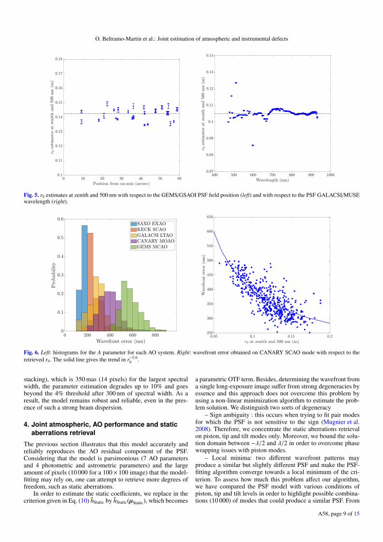
In addition, we highlight in Fig. 5 the r0 estimates at zenithand 500 nm obtained on a single image of GeMS/GSAOI anda single cube of GALACSI/MUSE. For the GEMS/GSAOI case,we have r0 measurements obtained from several PSFs distributedover the field. Given that r0 is assessed from the PSF wings thatcontain the non-AO-corrected spatial frequencies, we expect r0estimates to be independent of the PSF position in the FOV. Sim-ilarly, we multiplied r0 estimates obtained on GALACSI/MUSEimages by a factor (500/λc)6/5, where λc is the central wave-length of the considered image in the data cube, in order to dis-able the theoretical dependency of r0 with respect to λ.

A58, page 7 of 15

A&A 643, A58 (2020)

Table 3. Median and 1-σ standard-deviation of seeing values retrievedfrom the PSF-fitting process.

Observing site Median seeing 1-σ std

Mauna Kea 0.60′′ 0.13′′

Cerro Pachón 0.67′′ 0.09′′

Paranal 0.85′′ 0.15′′

La Palma 0.90′′ 0.22′′

Notes. Seeing values are given at zenith and 500 nm.

Using our model, we retrieve r0 as 14.2 cm± 0.4 and10.4 cm± 0.2 cm for GEMS/GSAOI and GALACI/MUSE,respectively. The achieved 3% 1-σ error of our estimatesshows that this method is robust and precise compared totelemetry-based techniques that typically reach 10% precision(Jolissaint et al. 2018).

For completeness, Fig. 6 shows histograms for the A param-eter (the wavefront error) and the function A = f (r0) for thespecific case of CANARY working in SCAO (i.e., the largestSCAO PSF dictionary we have). We clearly see that the wave-front standard-deviation error follows a r−5/6

0 law as we expectfrom the von Kármán PSD (von Karman 1948), which is pro-portional to r−5/3

0 for a SCAO system whose on-axis PSF is notinfluenced by the atmospheric turbulence profile. This illustratesthe agreement between the different retrieved parameters.

Moreover, the histogram of A estimates given in Fig. 6shows that the retrieved wavefront errors vary within a mean-ingful range: the SPHERE AO system performs better thanothers, as expected from such an extreme AO system, witha median of 140 nm, which includes all the aberrations thatblur the AO-corrected part of the PSF. The present SPHEREresults gather PSFs obtained with SPHERE/ZIMPOL, acquiredwith a AO loop running at low frequency (300 Hz, mV '11), and SPHERE/IRDIS fir which 25% were contaminatedby a strong LWE. Therefore, this wavefront error of 140nm seems consistent with the literature (Sauvage et al. 2016).The Keck AO system reaches 230 nm, which also complieswith Wizinowich (2012). From GALACSI/MUSE NFM images,we retrieve 285 nm of wavefront error, which agrees withthe Oberti et al. (2018) analysis Moreover, the GALACSI sys-tem was not yet fully optimized to operate in LTAO and arecent acquisition in 2019 already showed improvements onSR. For CANARY/CAMICAZ, we obtain a wavefront errors of320 nm, 396 nm and 417 nm in SCAO, MOAO, and GLAO moderespectively, which compares well with Martin et al. (2017) andVidal et al. (2014). Finally, GeMS/GSAOI data unveil a medianwavefront error of 570 nm from PSFs extracted from the field at20′′ up to 60′′ off-axis, which corresponds to a SR of 7.8% at theedges of the field and complies with analysis of the performanceof GeMS (Neichel et al. 2014; Rigaut et al. 2012).

We stress that this value of wavefront error is not deducedfrom the image SR but directly from the integral of thePSD, which can be determined from the model parameters(Fétick et al. 2019b). This corresponds to the real mathematicaldefinition of the wavefront error and is not influenced by theMaréchal approximation (Parenti & Sasiela 1994) that is biasedat low SR. Consequently, this model is also a robust focal plane-based wavefront error estimator.

3.4.2. Secondary parameters estimates

We have emphasized in Sect. 2 that parameters α and β governthe PSD shape and assist in the AO correction diagnosis.

Figure 7 presents histograms for each system; the β param-eter has a relatively narrow histogram with a peak located atβ = 1.82 and a 1-σ standard deviation of 0.6, while the αhistograms seem particularly instrument-dependent with val-ues from 0.001 rad.m for efficient AO correction to 1 rad.m formarginal AO correction (e.g., in the bluest visible wavelengthsof MUSE). Our first conclusion here is that an optimized AOsystem should provide a PSD with a β parameter comprisedbetween 1 and 1.9, as discussed in Sect. 2. For larger valuesof β, there is an excess of residual error into low-order spa-tial frequencies. For instance, we see that on Keck AO/NIRC2images the median β increases from 1.7 up to 2.1 in NGS andLGS modes, respectively, indicating the presence of additionallow-order modes introduced here mainly from the focal aniso-planatism (Wizinowich 2012; van Dam et al. 2006). In addition,we have observed cases with β > 2.5 on Keck data due to astrong wind-shake effect that was enlarging the PSF FWHM bya factor three compared to nominal performance. Both α and βparameters grow up in the presence of strong wind shake andare wavelength dependent as we see on GALACSI/MUSE his-tograms. However, from GEMS/GSAOI data analysis, we do notfind clear trend with respect to the field position, which may beowing to the uniform correction across the field provided by theMCAO mode of GEMS.

We illustrate here that those two parameters carry additionaland relevant information on the AO correction. However, theexact connection with the AO status is not straightforward toidentify. To enable this identification, we are currently develop-ing a convolutionnal neural network (Herbel et al. 2018) that wetrain to estimate the model parameters from the AO control loopdata, such as wavefront measurements. As we can collect a verylarge amount of data for the purpose of estimating a few tensof parameters, solving this problem is definitely achievable withdedicated simulations and on-sky data that we will continue tobe collected regularly among observatories.

3.5. Discussion on the influence of exposure time andspectral bandwidth

One of the major assumptions in the model proposed byFétick et al. (2019b) concerns the infinitely long exposurehypothesis. This model is therefore not capable of reproduc-ing atmospheric speckles that average when taking a sufficientlylong exposure. As the method relies on the second-order sta-tistical moment of the residual phase, the time necessary toachieve a convergence of the PSD shape is highly dependenton atmospheric parameters but may be achieved in few sec-onds (Martin et al. 2012). Thanks to SOUL/LUCI data, we ana-lyzed the PSF accuracy when fitted on short exposure imageswith integration times from 0.157 s to 60 s. We find that themodel matches the PSF down to 1–2 s of exposure and for aPSF acquired at 1.6 µm, below which the parameters estimationbegins to degenerate as illustrated in Fig. 8 (left) through theaverage of absolute parameters variations. We have also noticedthat the PSF shape remains stable from few seconds exposure,which explains the stability of retrieved parameters.

Moreover, using GALACSI/MUSE data, we tested the modelon a polychromatic image, from 2.5 nm up to 470 nm of spec-tral width by binning monochromatic PSF observed simultane-ously with MUSE. When compensating for the beam dispersion(recentering PSFs and then stack), the parameter estimation doesnot deviate by more than 4% over the whole spectral widthspan as presented in Fig. 8 (right). Consequently, the presenceof chromatic static aberrations and atmosphere chromaticity donot prevent the model from very accurate characterization of thePSF. When including the beam dispersion (no recentering before

A58, page 8 of 15

O. Beltramo-Martin et al.: Joint estimation of atmospheric and instrumental defects

Fig. 5. r0 estimates at zenith and 500 nm with respect to the GEMS/GSAOI PSF field position (left) and with respect to the PSF GALACSI/MUSEwavelength (right).

Fig. 6. Left: histograms for the A parameter for each AO system. Right: wavefront error obtained on CANARY SCAO mode with respect to theretrieved r0. The solid line gives the trend in r−5/6

0 .

stacking), which is 350 mas (14 pixels) for the largest spectralwidth, the parameter estimation degrades up to 10% and goesbeyond the 4% threshold after 300 nm of spectral width. As aresult, the model remains robust and reliable, even in the pres-ence of such a strong beam dispersion.

4. Joint atmospheric, AO performance and staticaberrations retrieval

The previous section illustrates that this model accurately andreliably reproduces the AO residual component of the PSF.Considering that the model is parsimonious (7 AO parametersand 4 photometric and astrometric parameters) and the largeamount of pixels (10 000 for a 100× 100 image) that the model-fitting may rely on, one can attempt to retrieve more degrees offreedom, such as static aberrations.

In order to estimate the static coefficients, we replace in thecriterion given in Eq. (10) h̃Static by h̃Static(µStatic), which becomes

a parametric OTF term. Besides, determining the wavefront froma single long-exposure image suffer from strong degeneracies byessence and this approach does not overcome this problem byusing a non-linear minimization algorithm to estimate the prob-lem solution. We distinguish two sorts of degeneracy

– Sign ambiguity : this occurs when trying to fit pair modesfor which the PSF is not sensitive to the sign (Mugnier et al.2008). Therefore, we concentrate the static aberrations retrievalon piston, tip and tilt modes only. Moreover, we bound the solu-tion domain between −λ/2 and λ/2 in order to overcome phasewrapping issues with piston modes.

– Local minima: two different wavefront patterns mayproduce a similar but slightly different PSF and make the PSF-fitting algorithm converge towards a local minimum of the cri-terion. To assess how much this problem affect our algorithm,we have compared the PSF model with various conditions ofpiston, tip and tilt levels in order to highlight possible combina-tions (10 000) of modes that could produce a similar PSF. From

A58, page 9 of 15

A&A 643, A58 (2020)

Fig. 7. Histograms for the β and α parameters for each system, as well as the averaged distribution.

Fig. 8. Left: average of absolute retrieved parameters with respect to the exposure time. The parameters are normalized by the value obtainedfrom the long-exposure PSF (60 frames). Error bars are assessed by averaging results over the SOUL/LUCI data sets. Right: average retrievedparameters normalized by the median value over the whole span with respect to the spectral width. The envelope shows the ±4% of variationsaround the median value and the spectral bandwidth is systematically centered around 700 nm. Error bars are assessed by averaging results overthe GALACSI/MUSE data sets.

a vector of aberrations, we have tested different permutationsof the elements of this vector and in 99% of cases, the rela-tive PSF variation is larger than 1%, which is large enough tochange the structure of the PSF and retrieve the correct wave-front map, as long as the S/N is sufficient (>50). We also relyon an analysis from Gerwe et al. (2008) that shows that for afit of 35 Zernike polynomials on a segmented pupil, there areno local minima as long as the initial guess for the static coef-ficient remains within ±0.2λ= 330 nm rms in H-band from theoptimal solution. We are in a situation where the static aberra-tions we attempt to retrieve are already mitigated from the Kecktelescope active control (Chanan et al. 1988) and the VLT spi-ders coating (Milli et al. 2018). Consequently, the aberrationslevel we must retrieve remains sufficiently weak to mitigate thepresence of local minima. At a level greater than 300 nm (KeckAO residual is 280 nm) would impact drastically the PSF anddegrade the telescope science exploitation so much that this

aberration would be necessarily visible and mitigated as much aspossible.

Henceforth, we are in a good situation to estimate piston, tipand tilt static modes on Keck and VLT images obtained on brightstar.

4.1. Keck cophasing error retrieval

The analysis presented in this section focuses on a smaller sam-ple of 129 Keck AO/NIRC2 data acquired in NGS mode andwith a high SR (>40%) in 2013 (Ragland et al. 2016). The resid-ual NCPA map was calibrated at the beginning of the night. Wecompared model-fitting performance in three situations: (i) a fitof PSD and photometric and astrometric parameters (11 values),(ii) a fit of these parameters when including, following Eq. (2),the static aberration map calibrated at the beginning of the nightand, (iii) a joint adjustment of the PSD, photometry/astrometry

A58, page 10 of 15

O. Beltramo-Martin et al.: Joint estimation of atmospheric and instrumental defects

Case 1 - February 2013 Case 2 - August 2013 Case 3 - September 2013

Skyimage

Model

Model+

NCPA

Model+

NCPA+

Cophasing

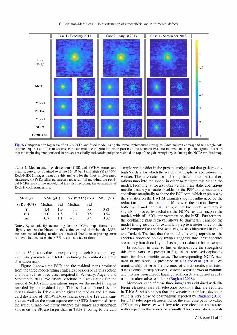
Fig. 9. Comparison in log scale of on-sky PSFs and fitted model using the three implemented strategies. Each column correspond to a single datasample acquired at different epochs. For each model configuration, we report both the adjusted PSF and the residual map. This figure illustratesthat the cophasing map retrieval improves drastically and consistently the residual on top of the gain brought by including the NCPA residual map.

Table 4. Median and 1-σ dispersion of SR and FWHM errors andmean square error obtained over the 129 H-band and high SR (>40%)Keck/NIRC2 images treated in this analysis for the three implementedstrategies: (i) PSD/stellar parameters retrieval, (ii) including the resid-ual NCPA map in the model, and (iii) also including the estimation ofKeck II cophasing errors.

Strategy ∆ SR (pts) ∆ FWHM (mas) MSE (%)

(SR> 40%) Median Std Median Std(i) 1.4 1.9 −0.9 0.8 0.81(ii) 1.0 1.8 −0.7 0.8 0.54(iii) 0.7 1.1 −0.5 0.4 0.32

Notes. Systematically, accounting for the NCPA map allows us toslightly reduce the biases on the estimates and diminish the MSE,but best model-fitting results are obtained thanks to cophasing errorretrieval that decreases the MSE by almost a factor three.

and the 36 piston values corresponding to each Keck pupil seg-ment (47 parameters in total), including the calibration staticaberration map.

Figure 9 shows the PSFs and the residual maps producedfrom the three model-fitting strategies considered in this sectionand obtained for three cases acquired in February, August, andSeptember, 2013. We firstly conclude that accounting for theresidual NCPA static aberrations improves the model fitting asrevealed by the residual map. This is also confirmed by theresults shown in Table 4 which gives the median and 1σ stan-dard deviation of SR/FWHM estimates over the 129 data sam-ples as well as the mean square error (MSE) determined fromthe residual map. We firstly observe that biases and dispersionvalues on the SR are larger than in Table 2, owing to the data

sample we consider in the present analysis and that gathers onlyhigh SR data for which the residual atmospheric aberrations areweaker. This advocates for including the calibrated static aber-rations map into the model in order to mitigate this bias in themodel. From Fig. 9, we also observe that these static aberrationsmanifest mainly as static speckles in the PSF and consequentlycontribute marginally to shape the PSF core, which explain whythe statistics on the FWHM estimates are not influenced by thereduction of the data sample. Moreover, the results shown inboth Fig. 9 and Table 4 highlight that the model accuracy isslightly improved by including the NCPA residual map in themodel, with still 50% improvement on the MSE. Furthermore,the cophasing map retrieval allows to drastically enhance themodel-fitting results, for example by up to a factor three on theMSE compared to the first scenario, as also illustrated in Fig. 9and Table 4. The fact that the model efficiently reproduces thespeckles observed on sky images suggests that these specklesare mainly introduced by cophasing errors due to the telescope.

In addition, in order to further demonstrate the strength ofthis framework, we present in Fig. 10 the retrieved cophasingmaps for three specific cases. The corresponding NCPA mapused in the model is presented in Ragland et al. (2016). Weunmistakably observe the presence of a stair mode, that intro-duces a constant step between adjacent segment rows or columnsand that has been already highlighted from data acquired in 2017using an alternative technique (Ragland 2018).

Moreover, each of those three images was obtained with dif-ferent elevation-azimuth telescope positions that are reportedin Table 5, which shows that the wavefront standard deviationvalue is very close to observations reported by Ragland (2018)for a 45◦ telescope elevation. Also, the stair case peak-to-valley(PV) energy increases with low telescope elevation and rotateswith respect to the telescope azimuth. This observation reveals

A58, page 11 of 15

A&A 643, A58 (2020)

Fig. 10. Retrieved cophasing maps in nm from PSFs acquired during three different epochs in 2013. The telescope elevation and azimuth wererespectively (79,240), (85,−82) and (43,240) from left to right.

Table 5. Summary of peak-to-valley (PV) and 1-σ standard deviationof retrieved cophasing error map regarding the corresponding telescopeelevation/azimuth.

Case Elevation/Azimuth (◦) PV (nm) Std (nm)

Feb. 2013 (79,240) 760 95Aug. 2013 (85,−82) 530 66Sept. 2013 (43,240) 1030 118

a connection between the presence of this stair mode and globalflexure over the primary mirror that is controlled to compensatefor the gravity effect. Deeper analyses will confirm the presenceof such a residual flexure on the Keck telescoped and whether ornot this framework now to allow us to correct for this stair modeto generally improve the scientific exploitation of the Keck, butalso future segmented telescopes.

Measuring the piston map from the focal-plane image is fea-sible from results obtained with the present analysis, but neces-sitates to have a star bright enough in the field to calibrate theseaberrations. We must ensure that the shape of the primary mirroris controlled without the aid of a focal-plane-based technique inorder to achieve the best image quality regardless of the observedfield. We are again in a situation where we have to retrieve a fewparameters (47) from a potentially large amount of data deliveredby segment position sensors, temperature, pressure and humid-ity sensors, atmospheric parameters near the dome and even AOtelemetry, which can deliver information about the piston errorwhen using a pyramid WFS (Bond et al. 2018b; Schwartz et al.2018). It is not easy to investigate the connection between thisensemble of data and the piston map, and the use of neural net-works for this purpose will be explored.

4.2. SPHERE low wind effect retrieval

The analysis presented in this section focuses on 176 SPHERE/IRDIS data obtained with good SR conditions (>40%) so as totest two different fitting strategies, namely (i) fitting the PSD andphotometry/astrometry parameters (11 parameters) and (ii) fit-ting these latter 11, and 12 additional parameters correspond-ing to piston, tip, and tilt of each VLT pupil area delimitedby the spiders in order to account for the LWE. According toSauvage et al. (2016), this description of the LWE allows themain impact of this effect to be reproduced, i.e., a strong PSFasymmetry.

Figure 11 presents the results of the two strategies imple-mented in our study over three particular cases for which a strongLWE is observed. We observe, especially in Fig. 11, that the soleparametrization of the PSD is not rich enough to precisely repro-duce the strong asymmetry, which becomes a solved problemthanks to the aberration parametrization we propose. Regardingthe estimated PSF shape and values given in Table 6, we showclear evidence that (i) describing the LWE as a combination ofdifferential piston, tip, and tilt allows to accurately characterizethe PSF asymmetry, and (ii) accounting for this description in thePSF model ensures that biases and dispersion on SR and FWHMestimates are drastically mitigated. Moreover, the average MSEvalue over the 176 data samples is significantly diminished, thatis, by a factor two. On the three cases illustrated in Fig. 11,Table 7 also reports the SR and FWHM errors as well as theMSE obtained from the PSF-fitting. These results show clearlya gain on accuracy for these particular cases for which the LWEimpact on the PSF is significant comparatively to the statisticaltrend observed on the 176 data sets. This gain is partially miti-gated on the statistical analysis owing to the fact that only 25% ofthe data were noticeably contaminated by the LWE. Moreover,the atmospheric part of the PSF model can mimic PSF asym-metries by modifying the ratio αx/αy in Eq. (7). Despite it leadsto an inaccurate representation of the LWE impact on the PSF,it permits to mitigate the SR and FWHM estimation error com-paratively to a symmetric atmospheric PSF model. As a sum-mary, fitting the twelve extra parameters to represent the LWEallows can enhance the PSF metrics estimation by a factor up tofive.

In order to confirm the robustness of the LWE retrieval, wehave compared the estimated static aberration map with ZELDAmeasurements (Vigan et al. 2019) taken during SPHERE com-missioning nights in 2014. The PSF-fitting was performed usingthe differential tip-tilt sensor (DTTS) that delivers 32× 32 pix-els images (Baudoz et al. 2010; Sauvage et al. 2015) acquiredsimultaneously with SPHERE/IRDIS using the ZELDA focal-plane mask to measure optical aberrations within the pupil-plane. Moreover, in order to calibrate ZELDA measurements(that are in ADU) to reconstruct the phase, we followedthe process described by Sauvage et al. (2015) and removedthe mean ADU value over the pupil and adjusted a multi-plicative factor to obtain the closest PSF possible from theDTTS observation as reported in Fig. 12. According to thiscalibration, we obtained standard deviations of 173 nm rmsand 146 nm rms on the ZELDA map and the DTTS image-based map,respectively, which leads to a quadratic difference

A58, page 12 of 15

O. Beltramo-Martin et al.: Joint estimation of atmospheric and instrumental defects

Case 1 Case 2 Case 3

Skyimage

Model

Model+

LWE

Fig. 11. Comparison in log scale of on-sky PSFs and fitted model considering the LWE or not. Each column correspond to a single data sampleacquired at different epoch. For each model configuration, we report both the adjusted PSF and the residual map. This figure illustrates that theLWE retrieval, modelled by a differential piston, tip and tilt improves drastically and consistently the residual map.

Table 6. Median and 1-σ dispersion of SR and FWHM errorsobtained over the 176 H-band and high SR (>40%) SPHERE/IRDISimages treated in this analysis for the two implemented strategies: (i)PSD/stellar parameters retrieval only (11 parameters in total) and (ii)including piston, tip, and tilt retrieval for the four pupil segments (23parameters in total).

Strategy ∆ SR (pts) ∆ FWHM (mas) MSE

(SR>40%) Median std Median stdNo LWE 0.5 1.9 −0.2 1.2 1.5

With LWE 0.2 1.0 −0.1 1.0 0.7

Notes. Systematically, accounting for the LWE model allows us toreduce the biases and the dispersion on PSF estimates.

of 92 nm rms. This residual includes the internal aberrations inthe IRDIS science path that do not impact the DTTS imagesand reach 50 nm and standard deviation (Beuzit et al. 2019).Also, this residual is likely mostly due to higher order aber-rations not included in the differential piston, tip, and tilt ofthe static map model, which suggests that further improve-ments can be pursued to characterize the LWE. In conclusion,the framework presented in this paper is a powerful tool toassist in the estimation of internal aberrations. Furthermore,we are able to assess these aberrations from the DTTS imagethat delivers a post-AO and non-coronagraphic image regard-less the coronagraphic mask employed during SPHERE/IRDISobservations. Consequently, this technique allows the joint esti-mation of atmospheric and instrumental defects using tip-tiltsensors measurements. Future work will address the extensionof this strategy to ELT instruments that will rely on a 2 × 2Shack-Hartmann WFS to measure low-order modes and thatwill provide PSFs from which we will be able to assess thetelescope aberrations and calibrate a PSF model for scienceexploitation.

Table 7. Impact of the LWE fit compared to a pure atmospheric modelon SR, FWHM and MSE metrics for the three cases presented inFig. 11.

Case LWE ∆ SR (pts) ∆ FWHM (mas) MSE (%)

1 No −1.3 1.5 1.7Yes −0.3 0.3 0.2

2 No 0.1 0.4 1.6Yes 0.04 0.1 0.3

3 No 0.8 −1.5 2.1Yes 0.6 −1.4 0.4

5. ConclusionsThis paper revisits and improves the analytical frameworkproposed by Fétick et al. (2019b), which now includes aparametrization of static aberrations for a joint retrieval of atmo-spheric parameters, AO performance and static aberrations.

We demonstrate in an exhaustive manner, using 4812 PSFsobtained from four different observatories and seven optical orNIR instruments, that the proposed model matches the PSF ofany AO flavor within 4% error, even for high-SR observations.We also illustrate that the retrieved parameters carry relevantinformation about the AO performance and the atmospheric con-ditions, especially seeing and wavefront error, that shows agree-ment with the literature.

Finally, we illustrate that this model, upgraded with addi-tional degrees of freedom to estimate static aberrations, allowsthe atmospheric parameters, AO performance and static aberra-tions, to be retrieved simultaneously. Particularly, the frameworkpresented in this paper allows us to assess (i) the Keck pupil seg-ment piston errors and especially the presence of a stair modethat was already pointed out (Ragland 2018) and, (ii) the LWEon SPHERE/IRDIS images as a combination of differential pis-ton, tip and tilt over the four VLT pupil segments delimited bythe spiders.

A58, page 13 of 15

A&A 643, A58 (2020)

Fig. 12. Top: from left to right: ZELDA measurements (114 nm std), retrieved static map (140 nm) from the PSF-fitting and residual (70 nm std)in nm. This comparison emphasizes the meaningfulness of the PSF-fitting outputs, which compares very well with dedicated measurements of theLWE. Bottom: from left to right: on-sky DTTS image, best-fitted PSF, ZELDA-based PSF.

This model is a unique tool that gathers an AO diagnosis anda PSF estimation facility in the simplest and the most parsimo-nious way possible. However, we have handled it as a parametricmodel so far and the next step of this work is to enable a for-ward estimation of its parameters from contextual data expectthe focal-plane image. We emphasized that the connection ofthese parameters with the observing conditions is not easilymade; nevertheless, thanks to the parsimony of this model, thisregression problem consists in assessing a few parameters (upto a few tens) from a large amount of data, which is providedby the AO telemetry, all the sensors within the telescope andthe dome and the external meteorological profilers, which canbe achieved with the use of neural networks. We are currentlydeveloping convolutional neural networks capable of directlyestimating the model outputs from either an imaged PSF or asubsample of AO telemetry and we will present this work in adedicated publication.

Acknowledgements. This work has been partially funded by the FrenchNational Research Agency (ANR) program APPLY – ANR-19-CE31-0011. Thiswork also benefited from the support of the WOLF project ANR-18-CE31-0018of the and the OPTICON H2020 (2017-2020) Work Package 1. This work hasmade use of the SPHERE Data Centre, jointly operated by OSUG/IPAG (Greno-ble), PYTHEAS/LAM/CeSAM (Marseille), OCA/Lagrange (Nice) and Observa-toire de Paris/LESIA (Paris) and supported by a grant from Labex OSUG@2020(Investissements d’avenir – ANR10 LABX56). Authors thank G. Fiorentino(INAF), F. Kerber (ESO), D. Massari (U. Bologna, INAF, Kapteyn Astronom-ical Institute), J. Milli (IPAG), and E. Tolstoy (Kapteyn Astronomical Insti-tute) to have conducted the SPHERE/ZIMPOL observations of NGC 6121 in2018 and provided the data. Authors thank P. Vernazza (LAM) to have deliv-ered SPHERE/ZIMPOL PSF calibrators obtained during his large programme.Authors acknowledge the contribution of J. Milli (IPAG) to utilize the SPHEREData centre pipeline. Authors thank F. Cantalloube (MPIA) and M. N’Diaye

(Lagrange) to provide the APLC mask model. Authors thank Jean-FrançoisSauvage (ONERA/LAM) for providing SPHERE DTTS and ZELDA measure-ments that served in the Sect. 4.2. Authors thank Sam Ragland (W.M. KeckObservatory) for giving access to NIRC2 images obtained during PSF recon-struction engineering nights on Keck II. Author thank G. Agapito (INAF) and E.Pinna (INAF) to communicate SOUL/LUCI commissioning data. Authors thankJ. Vernet (ESO) and S. Oberti (ESO) for providing MUSE NFM commissioningdata. Authors thank M. Andersen (Gemini), G. Sivo (Gemini) and A. Shugart(Gemini) for communicating GeMS/GSAOI observations of Trumpler 14 andsupporting the data processing. Author express their gratitude to F. Pedreros-Bustos (LAM) for a fruitful revision of the manuscript.

ReferencesArsenault, R., Madec, P. Y., Hubin, N., et al. 2008, Proc. SPIE, 7015, 701524Bacon, R., Accardo, M., Adjali, L., et al. 2010, Proc. SPIE, 7735, 773508Baudoz, P., Dorn, R. J., Lizon, J.-L., et al. 2010, Proc. SPIE, 7735, 77355BBeltramo-Martin, O., Correia, C. M., Ragland, S., et al. 2019, MNRAS, 487,

5450Beltramo-Martin, O., Marasco, A., Fusco, T., et al. 2020, MNRAS, 494, 775Benfenati, A., La Camera, A., & Carbillet, M. 2016, A&A, 586, A16Bertin, E., & Arnouts, S. 1996, A&A, 117, 393Beuzit, J. L., Vigan, A., Mouillet, D., et al. 2019, A&A, 631, A155Blanc, A., Fusco, T., Hartung, M., Mugnier, L. M., & Rousset, G. 2003, A&A,

399, 373Bond, C. Z., Correia, C. M., Sauvage, J.-F., et al. 2018a, Proc. SPIE, 10703,

107034MBond, C. Z., Wizinowich, P., Chun, M., et al. 2018b, Proc. SPIE, 10703, 107031ZBouché, N., Carfantan, H., Schroetter, I., Michel-Dansac, L., & Contini, T. 2015,

AJ, 150, 92Chanan, G. A., Mast, T. S., & Nelson, J. E. 1988, Very Large Telescopes and

their Instrumentation, 1, 421Claudi, R., Giro, E., Turatto, M., et al. 2014, Proc. SPIE, 9147, 91471LClénet, Y., Lidman, C., Gendron, E., et al. 2008, Proc. SPIE, 7015, 701529Conan, R., van Dam, M., Vogiatzis, K., Das, K., & Bouchez, A. 2019, Sixth

International Conference on Adaptive Optics for Extremely Large Telescopes,70

A58, page 14 of 15

O. Beltramo-Martin et al.: Joint estimation of atmospheric and instrumental defects

Conn, A., Gould, N., & Toint, P. 2000, Trust Region Methods, MPS-SIAMSerieson Optimization (Society for Industrial and Applied Mathematics)

Correia, C. M., & Teixeira, J. 2014, J. Opt. Soc. Am. A, 31, 2763Davies, R., Schubert, J., Hartl, M., et al. 2016, Proc. SPIE, 9908, 99081ZDelorme, P., Meunier, N., Albert, D., et al. 2017, in SF2A-2017: Proceedings of

the Annual meeting of the French Society of Astronomy and Astrophysics,eds. C. Reylé, P. Di Matteo, F. Herpin, et al.

Diolaiti, E., Bendinelli, O., Bonaccini, D., et al. 2000, Astrophysics Source CodeLibrary [record ascl: 0011.001]

Dohlen, K., Langlois, M., Saisse, M., et al. 2008, Proc. SPIE, 7014, 70143LDrummond, J. D. 1998, in Society of Photo-Optical Instrumentation Engineers

(SPIE) Conference Series, eds. D. Bonaccini, & R. K. Tyson, Proc. SPIE,3353, 1030

Epinat, B., Amram, P., Balkowski, C., & Marcelin, M. 2010, MNRAS, 401, 2113Exposito, J. 2014, PhD Thesis, Université Paris Diderot, FranceFauvarque, O., Neichel, B., Fusco, T., Sauvage, J.-F., & Girault, O. 2016, Optica,

3, 1440Ferreira, F., Gendron, E., Rousset, G., & Gratadour, D. 2018, A&A, 616, A102Fétick, R. J., Jorda, L., Vernazza, P., et al. 2019a, A&A, 623, A6Fétick, R. J. L., Fusco, T., Neichel, B., et al. 2019b, A&A, 628, A99Fétick, R. J. L., Mugnier, L. M., Fusco, T., & Neichel, B. 2020, MNRAS, 496,

4209Flicker, R. C., & Rigaut, F. J. 2005, J. Opt. Soc. Am. A, 22, 504Fried, D. L. 1966, J. Opt. Soc. Am. (1917–1983), 56, 1380Fried, D. L. 1982, J. Opt. Soc. Am. (1917–1983), 72, 52Fusco, T., Mugnier, L. M., Conan, J. M., et al. 2003, in Society of Photo-Optical

Instrumentation Engineers (SPIE) Conference Series, eds. P. L. Wizinowich,D. Bonaccini, et al., Proc. SPIE, 4839, 1065

Fusco, T., Sauvage, J. F., Mouillet, D., et al. 2016, Proc. SPIE, 9909, 99090UFusco, T., Bacon, R., Kamann, S., et al. 2020, A&A, 635, A208Gendron, E., Clénet, Y., Fusco, T., & Rousset, G. 2006, A&A, 457, 359Gendron, E., Morris, T., Hubert, Z., et al. 2010, in Adaptive Optics Systems II,

eds. B. Ellerbroek, M. Hart, N. Hubin, P. Wizinowich, Proc. SPIE, 7736Gerwe, D., Johnson, M., & Calef, B. 2008, Advanced Maui Optical and Space

Surveillance Technologies Conference, E28Gilles, L., Wang, L., & Boyer, C. 2018, Proc. SPIE, 10703, 1070349Gratadour, D., Puech, M., Vérinaud, C., et al. 2014, Proc. SPIE, 9148, 91486OHammer, F., Morris, S., Kaper, L., et al. 2016, in Ground-based and Airborne

Instrumentation for Astronomy VI, Proc. SPIE, 9908, 990824Herbel, J., Kacprzak, T., Amara, A., Refregier, A., & Lucchi, A. 2018, JCAP,

2018, 054Hippler, S., Feldt, M., Bertram, T., et al. 2019, Exp. Astron., 47, 65Hirst, P., & Cardenes, R. 2017, in Astronomical Data Analysis Software and

Systems XXV, eds. N. P. F. Lorente, K. Shortridge, & R. Wayth, ASP Conf.Ser., 512, 53

Jia, P., Wu, X., Yi, H., Cai, B., & Cai, D. 2020, AJ, 159, 183Jolissaint, L. 2010, J. Eur. Opt. Soc. Rapid Publ., 5, 10055Jolissaint, L., Mugnier, L. M., Neyman, C., Christou, J., & Wizinowich, P. 2012,

Proc. SPIE, 8447, 844716Jolissaint, L., Ragland, S., & Wizinowich, P. 2015, Adaptive Optics for

Extremely Large Telescopes IV (AO4ELT4), E93Jolissaint, L., Ragland, S., Christou, J., & Wizinowich, P. 2018, Appl. Opt., 57,

7837Kolmogorov, A. N. 1941, Akademiia Nauk SSSR Doklady, 32, 16Laginja, I., Leboulleux, L., Pueyo, L., et al. 2019, Proc. SPIE, 11117, 1111717Lai, O., Withington, J. K., Laugier, R., & Chun, M. 2019, MNRAS, 484, 5568Laidlaw, D. J., Osborn, J., Morris, T. J., et al. 2019, MNRAS, 483, 4341Lamb, M., Norton, A., Macintosh, B., et al. 2018, Proc. SPIE, 10703, 107035MLeboulleux, L., Sauvage, J.-F., Pueyo, L. A., et al. 2018, J. Astron. Telescopes

Instrum. Syst., 4, 035002Martin, O., Gendron, E., Rousset, G., & Vidal, F. 2012, in Adaptive Optics

Systems III, Proc. SPIE, 8447, 84472AMartin, O., Gendron, E., Rousset, G., et al. 2013, in Adaptive Optics for

Extremely Large Telescopes, Florence, Italy, ed. C. Kidon, 3rd AO4ELT conf.Martin, O. A., Correia, C. M., Gendron, E., et al. 2016a, J. Astron. Telescopes

Instrum. Syst., 2, 048001Martin, O. A., Correia, C. M., Gendron, E., et al. 2016b, Proc. SPIE, 9909,

99093PMartin, O. A., Gendron, É., Rousset, G., et al. 2017, A&A, 598, A37Masciadri, E., Lombardi, G., & Lascaux, F. 2014, MNRAS, 438, 983Massari, D., Marasco, A., Beltramo-Martin, O., et al. 2020, A&A, 634, L5Milli, J., Kasper, M., Bourget, P., et al. 2018, Proc. SPIE, 10703, 107032AMiyashita, A., Takato, N., Usuda, T., Uraguchi, F., & Ogasawara, R. 2004,

in Society of Photo-Optical Instrumentation Engineers (SPIE) ConferenceSeries, eds. J. Oschmann, & M. Jacobus, Proc. SPIE, 5489, 207

Moffat, A. F. J. 1969, A&A, 3, 455Morris, T., Gendron, E., Basden, A., et al. 2013, in Proceedings of the Third

AO4ELT Conference, eds. S. Esposito, L. FiniMorris, T., Gendron, E., Basden, A., et al. 2014, in Adaptive Optics Systems IV,

Proc. SPIE, 9148, 1Mugnier, L. M., Fusco, T., & Conan, J.-M. 2004, J. Opt. Soc. Am. A, 21, 1841Mugnier, L. M., Sauvage, J.-F., Fusco, T., Cornia, A., & Dandy, S. 2008, Opt.

Express, 16, 18406Myers, R. M., Hubert, Z., Morris, T. J., et al. 2008, in Adaptive Optics Systems,

eds. P. W. N. Hubin, C. Max, Proc. SPIE, 7015N’Diaye, M., Vigan, A., Dohlen, K., et al. 2016, A&A, 592, A79Neichel, B., Rigaut, F., Vidal, F., et al. 2014, MNRAS, 440, 1002Oberti, S., Kolb, J., Madec, P.-Y., et al. 2018, Proc. SPIE, 10703, 107031GO’Mahony, N. 2003, The Newsletter of the Isaac Newton Group of Telescopes,

7, 22Ono, Y. H., Akiyama, M., Oya, S., et al. 2016, J. Opt. Soc. Am. A, 33, 726Parenti, R. R., & Sasiela, R. J. 1994, J. Opt. Soc. Am. A, 11, 288Pinna, E., Esposito, S., Hinz, P., et al. 2016, Proc. SPIE, 9909, 99093VPuech, M., Evans, C. J., Disseau, K., et al. 2018, Proc. SPIE, 10702, 107028RRagazzoni, R., & Farinato, J. 1999, A&A, 350, L23Ragland, S. 2018, in Ground-based and Airborne Telescopes VII, SPIE Conf.

Ser., 10700, 107001DRagland, S., Jolissaint, L., Wizinowich, P., et al. 2016, in Adaptive Optics

Systems V, Proc. SPIE, 9909, 99091PRagland, S., Dupuy, T. J., Jolissaint, L., et al. 2018, in Adaptive Optics Systems

VI, Proc. SPIE, 10703, 107031JRigaut, F. J., Véran, J. P., & Lai, O. 1998, in Adaptive Optical System

Technologies, eds. D. Bonaccini, & R. K. Tyson, Proc. SPIE, 3353, 1038Rigaut, F., Neichel, B., Boccas, M., et al. 2012, Proc. SPIE, 8447, 84470IRigaut, F., Neichel, B., Boccas, M., et al. 2014, MNRAS, 437, 2361Robert, C., Fusco, T., Sauvage, J.-F., & Mugnier, L. 2008, Proc. SPIE, 7015,

70156ARoddier, F. 1981, Progress in Optics (Amsterdam: North-Holland Publishing

Co.), 19, 281Roddier, F. 1999, Adaptive Optics in Astronomy (Cambridge University Press)Sauvage, J. F., Fusco, T., LeMignant, D., et al. 2011, Second International

Conference on Adaptive Optics for Extremely Large Telescopes, 48, Onlineat http://ao4elt2.lesia.obspm.fr

Sauvage, J. F., Fusco, T., Guesalaga, A., et al. 2015, Adaptive Optics forExtremely Large Telescopes IV (AO4ELT4), E9

Sauvage, J.-F., Fusco, T., Lamb, M., et al. 2016, Proc. SPIE, 9909, 990916Schmid, H. M., Bazzon, A., Roelfsema, R., et al. 2018, A&A, 619, A9Schreiber, L., Diolaiti, E., Sollima, A., et al. 2012, Proc. SPIE, 8447, 84475VSchwartz, N., Sauvage, J.-F., Correia, C., et al. 2018, Proc. SPIE, 10703,

1070322Sitarski, B. N., Witzel, G., Fitzgerald, M., et al. 2014, in Adaptive Optics Systems

IV, Proc. SPIE, 9148Soummer, R. 2005, ApJ, 618, L161Stetson, P. B. 1987, PASP, 99, 191Ströbele, S., La Penna, P., Arsenault, R., et al. 2012, Proc. SPIE, 8447, 844737Thatte, N. 2017, Adaptative Optics for Extremely Large Telescopes VTokovinin, A., & Travouillon, T. 2006, MNRAS, 365, 1235Trujillo, I., Aguerri, J. A. L., Cepa, J., & Gutiérrez, C. M. 2001, MNRAS, 328,

977van Dam, M. A., Sasiela, R. J., Bouchez, A. H., et al. 2006, Proc. SPIE, 6272,

627231Vassallo, D., Farinato, J., Sauvage, J. F., et al. 2018, Proc. SPIE, 10705, 1070516Veran, J.-P., Rigaut, F., Maitre, H., & Rouan, D. 1997, J. Opt. Soc. Am. A, 14,

3057Vernazza, P., Brozv, M., Drouard, A., et al. 2018, VizieR Online Data Catalog:J/A+A/618/A154

Vidal, F., Gendron, E., & Rousset, G. 2010, JOSA A, 27, A253Vidal, F., Gendron, É., Rousset, G., et al. 2014, A&A, 569, A16Vigan, A., Moutou, C., Langlois, M., et al. 2010, MNRAS, 407, 71Vigan, A., N’Diaye, M., Dohlen, K., et al. 2019, A&A, 629, A11von Karman, T. 1948, Proc. Nat. Acad. Sci., 34, 530Wagner, R., Hofer, C., & Ramlau, R. 2018, J. Astron. Telescopes Instrum. Syst.,

4, 049003Witzel, G., Lu, J. R., Ghez, A. M., et al. 2016, in Proc. SPIE, Adaptive Optics

Systems V, 9909, 99091OWizinowich, P. 2012, in Adaptive Optics Systems III, Proc. SPIE, 8447, 84470DWizinowich, P. L., Acton, D. S., Lai, O., et al. 2000, in Adaptive Optical Systems

Technology, ed. P. L. Wizinowich, Proc. SPIE, 4007, 2Wizinowich, P. L., Le Mignant, D., Bouchez, A. H., et al. 2006, PASP, 118,

297

A58, page 15 of 15