Embed Size (px)
Citation preview
Selecting (In)Valid Instruments for InstrumentalVariables Estimation
Frank Windmeijera,e, Helmut Farbmacherb, Neil Daviesc,e
George Davey Smithc,e, Ian Whited
aDepartment of EconomicsUniversity of Bristol, UK
bCenter for the Economics of AgingMax Planck Institute Munich, Germany
cSchool of Social and Community MedicineUniversity of Bristol, UK
dMRC Biostatistics Unit, Cambridge, UKeMRC Integrative Epidemiology Unit, Bristol, UK
October 2015, Preliminary, please do not quote.
Abstract
We investigate the behaviour of the Lasso for identifying invalid instruments inlinear models, as proposed recently by Kang, Zhang, Cai and Small (2015, Journalof the American Statistical Association, in press), where invalid instruments aresuch that they enter the model as explanatory variables. We show that for thissetup, the Lasso may not select all invalid instruments in large samples if they arerelatively strong. Consistent selection also depends on the correlation structure ofthe instruments. We propose an initial estimator that is consistent when less than50% of the instruments are invalid, but its consistency does not depend on the rel-ative strength of the instruments or their correlation structure. This estimator cantherefore be used for adaptive Lasso estimation. We develop an alternative selec-tion method based on Hansen’s J-test of overidentifying restrictions, but limitingthe number of models to be evaluated. This latter selection procedure is consistentunder weaker conditions on the number of invalid instruments and is aligned withthe general identification result for this particular model.
1

1 Introduction
Instrumental variables estimation is a procedure for the identification and estimation
of causal effects of exposures on outcomes where the observed relationships are con-
founded by non-random selection of exposure. This problem is likely to occur in ob-
servational studies, but also in randomised clinical trials if there is selective participant
non-compliance. An instrumental variable (IV) can be used to solve the problem of non-
ignorable selection. In order to do this, an IV needs to be associated with the exposure,
but only associated with the outcome indirectly through its association with the exposure.
The former condition is referred to as the ‘relevance’and the latter as the ‘exclusion’.
Examples of instrumental variables are quarter-of-birth for educational achievement to
determine its effect on wages, see Angrist and Krueger (1991), randomisation of patients
to treatment as an instrument for actual treatment when there is non-compliance, see
e.g. Greenland (2000), and Mendelian randomisation studies use IVs based on genetic
information, see e.g. Lawlor et al. (2008). For recent reviews and further examples see
e.g. Clarke and Windmeijer (2012), Imbens (2014), Burgess et al. (2015) and Kang et
al. (2015).
Whether instruments are relevant can be tested from the observed association be-
tween exposure and instruments. The effects of ‘weak instruments’, i.e. the case where
instruments are only weakly associated with the exposure of interest have been derived for
the linear model using weak instrument asymptotics by Staiger and Stock (1997), leading
to critical values for the simple F-test statistic for testing the null of weak instruments,
derived by Stock and Yogo (2005).
In this paper we consider violations of the exclusion condition of the instruments,
following closely the setup of Kang et al. (2015) for the linear IV model where some of
the available instruments can be invalid in the sense that they can have a direct effect
on the outcomes or are associated with unobserved confounders. Kang et al. (2015)
propose a Lasso type procedure to identify and select the set of invalid instruments. Liao
(2013) and Cheng and Liao (2015) also considered shrinkage estimation for identification
of invalid instruments, but in their setup there is a subset of instruments that is known
to be valid and that contains suffi cient information for identification and estimation of
the causal effects. In contrast, Kang et al. (2015) do not assume any prior knowledge of
2

which instruments are potentially valid or invalid. This is a similar setup as in Andrews
(1999) who proposed a selection procedure using information criteria based on the so-
called J-test of over-identifying restrictions, as developed by Sargan (1958) and Hansen
(1982). The Andrews (1999) setup is more general than the Kang et al. (2015) setup
and requires a large number of model evaluations, which has a negative impact on the
performance of the selection procedure.
In this paper we assess the performance of the Kang et al. (2015) Lasso type selection
and estimation procedure. By evaluating the LARS algorithm of Efron et al. (2004), us-
ing large sample asymptotics, we show that the Lasso method may not consistently select
the correct invalid instruments. Consistent selection depends on the relative strength of
the instruments and/or the instrument correlation structure, even when less than 50%
of the instruments are invalid. We show that under the latter condition a simple median
type estimator is a consistent estimator for the parameters in the model, independent
of the relative strength of the instruments or their correlation structure. This estimator
can therefore be used for an adaptive Lasso procedure as proposed by Zou (2006). We
also show that the specific model structure of Kang et al. (2015) makes upward and
downward testing procedures as proposed by Andrews (1999) feasible, as the number of
models to be evaluated is limited by the model structure. These latter procedures result
in consistent model selection under weaker conditions on the number of invalid instru-
ments, with the necessary condition being that the valid instruments form the largest
group, where a group of instruments is formed by instruments giving the same value of
the estimate of the causal effect.1
Instrument strength is very likely to vary by instruments, so it will be important to
use our proposed estimators and selection methods for assessing instrument validity. In
Mendelian randomization studies it is clear that genetic markers have differential impacts
on exposures from examining the results from genome wide association studies. The
issue of correlation between genetic markers seems less of an issue as genes are generally
independently distributed by Mendel’s second law.
Finally, another strand of the literature focuses on instrument selection in potentially
1Bowden et al. (2015) and Kolesar et al. (2015) allow for all instruments to be invalid and show thatthe causal effect can be consistently estimated if the number of instruments increases with the samplesize under the relatively strong assumption of uncorrelatedness of the instrument strength and theirdirect effects on the outcome variable.
3

high-dimensional settings, see e.g. Belloni et al. (2012) and Lin et al. (2015). Here the
focus is on identifying important covariate effects and selecting optimal instruments from
a (large) set of a priori valid instruments, where optimality is with respect to the variance
of the IV estimator. Belloni et al. (2012) propose a new method for selecting the Lasso
penalty parameter. We analyse its behaviour for the Lasso selection method in cases
where this method consistently selects the instruments. As our setting is that of a fixed
number of potential instruments, we show that simply using Hansen’s J-test performs
as well, and that the so-called post-Lasso selection IV estimator has better finite sample
properties than the Lasso estimator.
2 Model and sisVIVE Estimator
We follow Kang, Zhang, Cai and Small (2015) (KZCS from now on), who considered the
following potential outcomes model. The outcome for an individual i is denoted by the
scalar Yi, the treatment by the scalar Di and the vector of L potential instruments by Zi..
The instruments may not all be valid and can have a direct or indirect effect resulting in
the following potential outcomes model
Y(d′,z′)i − y(d,z)i = (z′ − z)φ+ (d′ − d) β (1)
E[Y(0,0)i |Zi.
]= Z′i.ψ (2)
where φ measures the direct effect of z on Y , and ψ represents the effect of confounders
in the relationship between Zi. and Y(0,0)i .
We have a random sample Yi, Di,Z′i.
ni=1. Combining (1) and (2), the observed data
model for the random sample
Yi = Diβ + Z′i.α + εi (3)
where α = φ+ ψ;
εi = Y(0,0)i − E
[Y(0,0)i |Zi.
]and hence E [εi|Zi.] = 0. The KZCS definition of a valid instrument is then given as
follows: Instrument j, j ∈ 1, ..., L, is valid if αj = 0 and it is invalid if αj 6= 0. As
in the KZCS setting, we are interested in the identification and estimation of the scalar
treatment effect β in large samples with a fixed number L of potential instruments.
4

Let y and d be the n-vectors of n observations on Yi and Di respectively, andlet Z be the n× L matrix of potential instruments. As an intercept is implicitly presentin the model, y, d and the columns of Z have all been taken in deviation from their
sample means. Let Zsel be a subset of instruments included in the equation, and let
R =[
d Zsel
]. The standard Instrumental Variables, or Two-Stage Least Squares
(2SLS), estimator is then given by
θ =
(βαsel
)=(R′Z (Z′Z)
−1Z′R
)−1R′Z (Z′Z)
−1Z′y. (4)
Let d = PZd, PZ = Z (Z′Z)−1 Z′, then θ is equivalent to the OLS estimator in the model
Yi = Diβ + Z′sel,i.αsel + ξi
and hence
αsel =(Z′selMdZsel
)−1Z′selMdy
=(Z′selMdZsel
)−1Z′selMdPZy. (5)
where Md = In−Pd, where In is the identity matrix of order n.
d is the linear projection of d on Z. If we define γ = (Z′Z)−1 Z′d, then d = Zγ, or
Di = Z′i.γ, and we specify
Di = Z′i.γ + vi, (6)
where γ = E [Zi.Z′i.]−1E [Zi.Di], and hence E [Zi.vi] = 0. Further, as in KZCS, let
Γ = E [Zi.Z′i.]−1E [Zi.Yi] = γβ + α. Clearly, both γ and Γ can be consistently estimated
under standard assumptions. Assuming that γj 6= 0 ∀j, then define πj as
πj ≡Γjγj
= β +αjγj. (7)
Theorem 1 in KZCS states the conditions under which, given knowledge of γ and Γ, a
unique solution exists for values of β and αj . A necessary and suffi cient condition to
identify β and the αj is then that the valid instruments form the largest group, where
instruments form a group if they have the same value of π. Corollary 1 in KZCS then
states a suffi cient condition for identification. Let s be the number of invalid instruments,
then if s < L/2, the parameters are identified as then clearly the largest group is formed
by the valid instruments.
5

In model (3), some elements of α are assumed to be zero, but it is not known ex-ante
which ones they are and the selection problem therefore consists of correctly identifying
those instruments with non-zero α. KZCS propose to estimate the parameters α and β
by using `1 penalisation on α and to minimise(αλ, β
λ)
= arg minα,β
1
2‖PZ (y − dβ − Zα) ‖22 + λ‖α‖1, (8)
where the `1 norm ‖α‖1 =∑
j |αj| and the squared `2 norm is (y − dβ − Zα)′PZ (y − dβ − Zα).
This method is closely related to the Lasso, and the regularization parameter λ deter-
mines the sparsity of the vector αλ. From (5), a fast two-step algorithm is proposed that
runs as follows. For a given λ solve
αλ = arg minα
1
2‖MdPZy −MdZα‖
22 + λ‖α‖1 (9)
and estimate βλby
βλ
=d′(y − Zαλ
)d′d
. (10)
In order to find αλ in (9), the Lasso modification of the LARS algorithm of Efron,
Hastie, Johnstone and Tibshirani (2004) can be used and KZCS have developed an R-
routine for this purpose and call the resulting estimator sisVIVE (some invalid and some
valid IV estimator), where the regularisation parameter λ is obtained by cross-validation.
Following the notation of Zou (2006), let A be the set of invalid instruments, A =
j : αj 6= 0. Let An =j : αλj 6= 0
. We will first investigate under what conditions the
Lasso method consistently selects invalid instruments such that limn→∞ P (An = A) = 1,
or for a weaker version, such that limn→∞ P (An ⊇ A) = 1.
An important difference with the standard Lasso approach for linear models is that
the matrix of explanatory variables MdZ in (9) is not full rank, but its rank is equal to
L − 1. Whereas λ = 0 would simply include all regressors in the standard linear model
and the resulting OLS estimator is consistent, setting λ = 0 in (9) does not lead to a
unique 2SLS estimator, as all models with L − 1 instruments included as invalid would
result in a residual correlation of 0 and hence λ = 0. Therefore the LARS algorithm
has to start from a model without any instruments included as invalid, and at the last
LARS/Lasso step one instrument is excluded from the model, i.e. treated as valid. When
L− 1 instruments have been selected as invalid and included in the model, the resulting
6

Lasso estimator is the (just identified) 2SLS estimator and this final model is the model
for which λ = 0. Clearly, it can then be the case that the LARS/Lasso path is such that
it does not include a model where all invalid instruments have been selected as such,
which is the case when the final instrument selected as valid is in fact invalid. If that is
the case, then there is no value of λ for which βλ is consistent.
Below we show under what conditions the large sample, n → ∞, LARS/Lasso pathdoes or does not include models where all invalid instruments have been selected. In
simple settings, we show that this does depend on the number of invalid instruments, the
relative strengths of the invalid versus the valid instruments and the correlation structure
of the instruments. KZCS did show analytically that the performance of the Lasso esti-
mator is influenced by these factors. They derived an estimator performance guarantee
condition related to the values of µ = maxj 6=r∣∣Z′.jZ.r
∣∣ and ρ = maxj
∣∣∣Z′.jd∣∣∣ /d′d. Theconstant µ measures the maximum correlation between any two columns of the matrix of
instruments Z, and ρ is a measures the maximum strength of the individual instruments.
Their derived condition on the number of invalid instruments in Corollary 2 is that
s < min(
112µ, 110ρ2
). KZCS acknowledge the fact that these constraints are very strict.
For example, if µ = 0.1, then s < 10/12 and no invalid instruments are allowed, although
their Monte Carlo results show that a simple correlation structure does not affect the
behaviour of the estimator. Similarly for ρ, only a small value is allowed in order to have
any invalid instruments allowed in the setup. If we assume that plim (n−1Z′Z) = Q, then
plim
∣∣∣Z′.jd∣∣∣d′d
=
∣∣Q′.jγ∣∣γ′Qγ
.
Therefore, if Q = IL this is equal to∣∣γj∣∣ /γ′γ and hence ρ is associated with the strongest
instrument in terms of γj. Our results for consistent selection are based on the relative
values of γ for the valid and invalid instruments, where we simply refer to γj as the in-
strument strength for instrument j. We show for uncorrelated instruments, with Q = IL,
that if invalid instruments are stronger than the valid ones, the selection procedure may
select the valid instruments as invalid. Also, for the correlation structure, as in Zou
(2006), we show that consistent selection depends on the patterns of correlations, not
on the maximum correlation per se. Using our large sample analysis we can find simple
configurations where the Lasso selection is inconsistent, which we confirm in some Monte
7

Carlo studies.
In order to mitigate these problems for the Lasso estimator, one can use the Adaptive
Lasso approach of Zou (2006) using an initial consistent estimator of the parameters. In
the standard linear case, the OLS estimator in the model with all explanatory variables
included is consistent. As explained above, in the instrumental variables model this
option is not available. Let πj = Γj/γj, where γ = (Z′Z)−1 Z′d and Γ = (Z′Z)−1 Z′y.
Under standard assumptions as specified below, we show that the median of the πjs is a
consistent estimator for β when s < L/2, without any further restrictions on the relative
strengths or correlations of the instruments, and hence this estimator can be used for the
Adaptive Lasso.
We finally propose alternative consistent selection methods that are more closely
related to the identification results derived from (7). These are the so-called upward and
downward selection methods as proposed by Andrews (1999) based on the Hansen (1982)
J-test of overidentifying restrictions, using the rank-ordered estimates of πj to guide the
search.
As a further contribution, we consider different selection strategies to determine the
value of λ for the Lasso estimator (8) when suffi cient conditions are met for consistent
selection end estimation. We consider a method recently proposed by Belloni, Chen,
Chernozhukov and Hansen (2012) and a method based on Hansen’s J-test. We show that
these methods perform well, but that finite sample estimation results are substantially
better for post-Lasso selection 2SLS estimators than for the Lasso estimators.
For the random variables and sample Yi, Di,Z′i.
ni=1, and model (3) we assume
throughout that the following conditions hold:
C1. E [Zi.Z′i.] = Q is full rank
C2. plim (n−1Z′Z) = E [Zi.Z′i.]; plim (n−1Z′d) = E [Zi.Di]; plim (n−1Z′ε) = E [Zi.εi] = 0.
C3. γ = (E [Zi.Z′i.])−1E [Zi.Di], γj 6= 0, j = 1, ..., L.
3 Uncorrelated and Equal Strength Instruments
We first consider the conditions under which the Lasso procedure consistently selects
the invalid instruments for the case where the instrument strengths are all equal, i.e.
γj = γ for j = 1, .., L, and the instruments are uncorrelated, with variances equal to 1,
8

E [Zi.Z′i.] = IL = plim (n−1Z′Z).
Dividing by the sample size n, incorporating normalisation and noting that Z′MdMdPZy =
Z′Mdy, the Lasso estimator αλ is obtained as
αλ = arg minα
1
2n‖y − Zα‖22 +
λ
n‖Ωnα‖1, (11)
where Z = MdZ, and Ωn is an L × L diagonal matrix with diagonal elements ωj =√Z′j.Zj./n =
√Z′j.MdZj./n.
The Lasso path can be obtained using the Lasso modification of the LARS algorithm,
see Efron et al. (2004). Starting from the model without any instruments included as
explanatory variables, let the L-vector of correlations cn be defined as
cn = n−1Ω−1n Z′y = n−1Ω−1n Z′Mdy,
with j-th element
cn,j =n−1Z′.jMdy√n−1Z′.jMdZ.j
(12)
The first LARS step selects the variable(s) Z.j for which |cn,j| is maximum. We have forlarge samples that
plim (cn,j) =αj − α√
(L− 1) /L,
as
plim(n−1Z′.jMdy
)= plim
(n−1Z′.jMdZα
)= plim
(n−1Z′.jZα
)− plim
(n−1Z′.jPZd (d′PZd)
−1d′PZZα
)= αj − γj
γ′α
γ′γ= αj − L−1
L∑r=1
αr
= αj − α,
and
plim(n−1Z′j.MdZj.
)= 1−
γ2jγ′γ
= 1− 1
L
using the facts that plim (n−1Z′Z) = IL and that all the γjs are the same.
There are s < L invalid instruments. If all the invalid instruments have the same
effect a, the case considered mostly in the KZCS simulations, then α = sa/L. We then
9

get for a valid instrument plim (cn,val) = −sa/√L (L− 1), and for an invalid instru-
ment plim (cn,inv) = (L− s)a/√L (L− 1). In large samples, the invalid instruments get
therefore selected in the first LARS step if
(L− s) |a| > s |a| ⇔ s < L/2,
so less than 50% of the instruments can be invalid, which is aligned with Theorem 1 and
Corollary 1 of KZCS. In practice, of course, the correlations for the invalid (and valid
instruments) will not be exactly equal to each other, and the instruments will be selected
one at the time, with the LARS update of the predicted mean approaching zero for large
sample sizes within the two groups of instruments.
It is clear from the correlations derived above, that many situations can arise in terms
of selecting invalid instruments correctly, depending on the values of the αj’s. At the
one extreme, it is clear that the first LARS step would correctly select L − 2 invalid
instruments, for L even, when half of them have effect a and the other half −a, whichis a case where the parameters are in principle not identified. Perhaps more interesting
is to consider the situation where the s invalid instruments have distinct positive effects,
ordered in such a way that α1 > α2 > ... > αs > αs+1 = ... = αL = 0. We show in
the Appendix that also for this case the condition that s < L/2 need to be satisfied for
the LARS algorithm to select the invalid instruments in the first s steps in large samples
and that for s > L/2 the full LARS path does not include a model where all invalid
instruments have been included. This is in contrast to the identification results, as the
parameters are identified in this case by Theorem 1 in KZCS as long as s < L− 1.
For consistent model selection and estimation, the condition that s < L/2 is suffi cient
when instruments are uncorrelated and have equal strengths. We will show below that
this condition is no longer suffi cient when we allow for differential instrument strengths,
especially when invalid instruments are relatively strong. It is also not suffi cient under
certain correlation structures of the instruments, as observed by Zou (2006) for the stan-
dard linear model case. However, before we move to these problems, we will analyse the
behaviour of the Lasso estimator of (11) in situations where the condition that s < L/2
is suffi cient for consistent selection of the invalid instruments.
We start with presenting some estimation results from a simple Monte Carlo exercise,
10

similar to that in KZCS. The data are generated from
Yi = Diβ + Z′i.α + εi
Di = Z′i.γ + vi,
where (εivi
)∼ N
((00
),
(1 ρρ 1
));
Zi. ∼ N (0, IL) ;
and we set β = 0; γj = 0.2, j = 1, ..., L; L = 10; ρ = 0.25; s = 3, and the first s elements
of α are equal to a = 0.2. Table 1 presents estimation results for estimators of β in terms of
bias, standard deviation, rmse and median absolute deviation (mad) for 1000 replications
for sample sizes of n = 500, n = 2000 and n = 10, 000. The "2SLS" results are for the
2SLS estimator that treats all instruments as valid. The "2SLS or" is the oracle 2SLS
estimator that includes Z.1, .,Z.3 in the model as explanatory variables. For the Lasso
estimates, the value for λ has been obtained by 10-fold cross-validation, using the one-
standard error rule, as in KZCS, but we also present results for 10-fold cross validation
not using the one-standard error rule. The latter estimator is denoted "Lassocv", whereas
the former is denoted "Lassocvse", which is the one produced by sisVIVE. We also present
result for the so-called post-Lasso estimator, see e.g. Belloni et al. (2012), which is called
the LARS-OLS hybrid by Efron et al. (2004). In this case this is the 2SLS estimator (4),
where Zsel is the set of instruments with non-zero estimated Lasso coeffi cients. Further
entries in the table are the average number of selected instruments, which are the number
of instruments with non-zero α coeffi cients, together with the minimum and maximum
number of selected instruments, and the proportion of times the selected instruments
include the 3 invalid instruments.
11

Table 1. Estimation results for β; L = 10, s = 3
#sel instr prop Z.1, .,Z.3
β bias std dev rmse mad [min, max] selectedn = 5002SLS 0.2966 0.0808 0.3074 0.2944 0 02SLS or 0.0063 0.0843 0.0845 0.0570 3 1Lassocv 0.1384 0.0965 0.1687 0.1352 6.41 [2,9] 0.990Post-Lassocv 0.1169 0.1136 0.1630 0.1143Lassocvse 0.2206 0.0847 0.2363 0.2174 3.16 [0,8] 0.664Post-Lassocvse 0.0905 0.1243 0.1537 0.0994n = 20002SLS 0.3019 0.0387 0.3044 0.3007 0 02SLS or 0.0047 0.0422 0.0424 0.0285 3 1Lassocv 0.0721 0.0509 0.0882 0.0705 6.56 [3,9] 1Post-Lassocv 0.0617 0.0577 0.0845 0.0644Lassocvse 0.1140 0.0430 0.1218 0.1165 3.76 [3,8] 1Post-Lassocvse 0.0277 0.0521 0.0590 0.0387n = 10, 0002SLS 0.2996 0.0177 0.3002 0.2992 0 02SLS or 0.0006 0.0183 0.0183 0.0127 3 1Lassocv 0.0317 0.0236 0.0395 0.0311 6.44 [3,9] 1Post-Lassocv 0.0272 0.0267 0.0380 0.0282Lassocvse 0.0479 0.0187 0.0514 0.0489 3.81 [3,9] 1Post-Lassocvse 0.0118 0.0238 0.0265 0.0176Notes: Results from 1000 MC replications; a = 0.2; β = 0; γ = 0.2; ρ = 0.25
The results in Table 1 reveal some interesting patterns. First of all, the Lassocv esti-
mator outperforms the Lassocvse estimator in terms of bias, rmse and mad for all sample
sizes, but this is reversed for the post-Lasso estimators, i.e. the post-Lassocvse outper-
forms the post-Lassocv. The Lassocv estimator selects on average around 6.5 instruments
as invalid, which is virtually independent of the sample size. The Lassocvse estimator
selects on average around 3.8 instruments as invalid for n = 2000 and n = 10, 000, but
less, 3.17 for n = 500. Although the correct instruments are always selected for the larger
sample sizes, the Lassocvse is substantially biased, the biases being larger than twice the
standard deviations. The post-Lassocvse estimator performs best, but is still substantially
outperformed by the oracle 2SLS estimator.
Figures 1a and 1b shed some more light on the different behaviour of the Lasso and
post-Lasso estimators. Figure 1a shows the bias and standard deviations of the two
12

estimators for different values of λ/n, for the design above with n = 2000, again from
1000 replications. It is clear that the Lasso estimator exhibits a positive bias for all
values of λ, declining from that of the naive 2SLS estimator to the minimum bias of
0.0664 at λ/n = 0.0060. In contrast, the post-Lasso estimator has a (much) smaller
bias, obtaining its minimum bias of 0.0068 at the value of λ/n of 0.0965. Figure 1b
displays the same information but now as a function of the LARS steps (we have omitted
3 replications where there were Lasso steps). At step 3, the correct 3 invalid instruments
have been selected 991 times out of the 997 replications, and the post-Lasso estimator has
a bias there of 0.0058, only fractionally larger than that of the oracle 2SLS estimator. In
contrast, the Lasso estimator for β still has a substantial upward bias at step 3. Its bias
decreases from 0.116 at step 3 to a minimum of 0.0650 at step 8. Interestingly, the bias
of the post-Lasso estimator increases again after step 3, reaching the same bias as the
Lasso estimator at the last step, as there λ = 0 and the Lasso and post-Lasso estimators
are equal.
Figures 1a and 1b. Bias and standard deviations of Lasso and post-Lasso estimators as
functions of λ/n and LARS steps. Same design as in Table 1, n = 2000. 3 replications
out of 1000 omitted in 1b due to Lasso steps.
We can understand the different behaviour of the Lasso and post-Lasso estimators,
which is due to shrinkage of the Lasso estimator for α, as follows. Denote by Zλsel the
matrix of selected instruments for any value of λ, i.e. those instruments with non-zero
13

values of αλ. For the Lasso and post-Lasso estimators, βλand β, we have that
βλ
= β +d′Zλ
sel
(αsel − αλsel
)d′d
.
For those values of λ where the correct invalid instruments have been included, the biases
of β and α are small in large samples. Define δλas the shrinkage factor of the Lasso
estimator, relative to that of the post-Lasso estimator, i.e. αλsel ≈ δλαsel. We then have
approximately
βλ≈ β +
(1− δ
λ) d′Zλ
selαsel
d′d.
Note that in the model without any instruments included as explanatory variables, we
have for the 2SLS estimator,
β =d′y
d′d=
d′y
d′d= β +
d′Zα
d′d+
d′ξ
d′d
and so we see that the bias of the Lasso estimator due to shrinkage is in the direction of
the bias of the 2SLS estimator in the model without any included invalid instruments. As
an illustration, for the n = 2000 case above, at λ/n = 0.0965, the means of the first three
elements of αλsel are all equal to 0.067, whereas those of the post-Lasso 2SLS estimator
are equal to 0.198, hence 1 − δλ
= 0.662. The bias of the 2SLS estimator treating all
instruments as valid is given by 0.302, and 0.662∗0.302 = 0.200. This is very close to the
difference in the biases of βλand β at this point, which is given by 0.201−0.007 = 0.194.
3.1 Stopping Rule
It is clear from the results above that the post-Lasso estimator outperforms the Lasso
estimator, with the performance of the post-Lassocvse best, but still some way short of
that of the oracle 2SLS estimator, even for n = 10, 000. It is also clear, and easily
understood from Figures 1a and 1b, that the 10-fold cross-validation method selects
models that are too large in the sense that valid instruments get selected as invalid over
and above the invalid ones, and does not improve with increasing sample size, although
the ad hoc one-standard error rule does improve the selection. We next consider two
alternative stopping rules, one proposed for the Lasso by Belloni et al. (2012), and one
for GMM moment selection by Andrews (1999).
14

Belloni et al. (2012) explicitly allow for general conditional heteroskedasticity and
consider the Lasso estimator defined as
αλ = arg minα
1
2n‖y − Zα‖22 +
λ
n‖Ω∗nα‖1,
where Ω∗n is an L× L diagonal matrix with j-th diagonal element
ω∗n,j =
√√√√n−1n∑i=1
z2ij ε2i ,
where
εi = yi − Z′i.α.
Then let
c∗n =1
n
n∑i=1
(Ω∗n
)−1Zi.εi.
Belloni et al. (2012) apply the moderate deviation theory of Jing, Shao and Wang (2003)
to bound deviations of the maximal element of the vector of correlations c∗n and hence
λ/n for models that have selected the invalid instruments. They establish that
P(√
nmax (c∗n) ≤ Φ−1(
1− τn2L
))≥ 1− τn + o (1) ,
where Φ−1 (.) is the inverse, or quantile function, of the standard normal distribution,
and that the penalty level should satisfy
P
(λ
n≥ qmax (c∗n)
)→ 1
for some constant q > 1. Belloni et al. (2012) then recommend selecting
λ
n= qΦ−1
(1− τn
2L
)/√n
and to set the confidence level τn = 0.1/ ln (n) and the constant q = 1.1. For n = 2000,
this results in a value for λ/n equal to 0.079, which suggests a good performance of the
post-Lasso estimator from Figure 1a, as the design there is conditionally homoskedastic.
We obtain the Lasso and post-Lasso estimators using the Belloni et al. (2012) iterative
procedure as described in their Appendix A, as the εi need to be estimated to construct
Ω∗n. We use the post-Lasso estimator at every step to estimate the εi.
15

The second stopping rule we consider is based on the approach of Andrews (1999).
We can use this approach because the number of instruments L is fixed and (much)
smaller than n. Consider again the model
y = dβ + Zselαsel + ξ (13)
= Rθ + ξ.
Let Gn (θ) = n−1Z′ (y −Rθ), then the Generalised Methods of Moment (GMM) estima-
tor is defined as
θGMM = arg minθ
Gn (θ) W−1n Gn (θ) ,
see Hansen (1982). 2SLS is a one-step GMM estimator, settingWn = n−1Z′Z. Given the
moment conditions E (Zi.ξi) = 0, 2SLS is effi cient under conditional homoskedasticity,
E(ξ2i |Zi.
)= σ2ξ . Under general forms of conditional heteroskedasticity, an effi cient two-
step GMM estimator is obtained by setting
Wn = Wn
(θ1
)= n−1
n∑i=1
((yi −R′i.θ1
)2Zi.Z
′i.
)where θ1 is an initial consistent estimator, with a natural choice the 2SLS estimator.
Then, under the null that the moment conditions are correct, E (Zi.ξi) = 0, the Hansen
(1982) J-test statistic and its limiting distribution are given by
Jn
(θ1
)= nGn
(θ2
)W−1
n
(θ1
)Gn
(θ2
)d→ χ2(L−dim(R)).
We can now combine the LARS/Lasso algorithm with the Hansen J-test, which is then
akin to a directed downward testing procedure in the terminology of Andrews (1999).
Let the critical value ζn,k = χ2k (τn) be the 1− τn quantile of the χ2k distribution, wherek = L − dim (R). Compute at every LARS/Lasso step as described above the Hansen
J-test and compare it to the corresponding critical value. We then select the model with
the largest degrees of freedom for which the J-test is smaller than the critical value. If
two models of the same dimension pass the test, which can happen with a Lasso step,
the model with the smallest value of the J-test gets selected. Clearly, this approach is a
post-Lasso approach, where the LARS algorithm is purely used for selection of the invalid
instruments. For consistent model selection, the critical values ζn,k need to satisfy
ζn,k →∞ and ζn,k = o (n) , (14)
16

see Andrews (1999). We select τn = 0.1/ ln (n) as per the Belloni et al. (2012) method.
Table 2 presents the estimation results using the two alternative stopping rules.
The subscripts "bcch" and "ah" denote the Belloni et al. (2012) method and the An-
drews/Hansen approach respectively. Both post-Lasso estimators are the simple 2SLS
estimators for comparison with the results in Table 1.
Table 2. Estimation results for β; L = 10, s = 3
#sel instr prop Z.1, .,Z.3
β bias std dev rmse mad [min, max] selectedn = 500Lassobcch 0.2770 0.0846 0.2896 0.2770 1.16 [0,4] 0.068Post-Lassobcch 0.1914 0.1324 0.2327 0.2028Post-Lassoah 0.0896 0.1252 0.1539 0.1007 2.56 [0,5] 0.3912SLS or 0.0063 0.0843 0.0845 0.0570 3 1n = 2000Lassobcch 0.1688 0.0438 0.1744 0.1694 3.11 [3,5] 1Post-Lassobcch 0.0091 0.0445 0.0454 0.0294Post-Lassoah 0.0055 0.0430 0.0434 0.0286 3.02 [3,5] 12SLS or 0.0047 0.0422 0.0424 0.0285 3 1n = 10, 000Lassobcch 0.0751 0.0180 0.0772 0.0756 3.11 [3,5] 1Post-Lassobcch 0.0027 0.0191 0.0193 0.0134Post-Lassoah 0.0009 0.0186 0.0186 0.0129 3.02 [3,5] 12SLS or 0.0006 0.0183 0.0183 0.0127 3 1Notes: Results from 1000 MC replications; a = 0.2; β = 0; γ = 0.2 ρ = 0.25
For n = 500, we find that the value of λ/n as determined by the BCCH method is too
large and the method selects too few instruments as invalid, resulting in severely biased
Lasso and post-Lasso estimates. The AH approach behaves better for n = 500, but it also
selects too few invalid instruments, resulting in an upward bias for this particular case,
which is similar to results for the post-Lassocvse estimator in Table 1. For n = 2000 and
n = 10, 000, both post-Lasso procedures perform very well with properties very similar
to that of the oracle 2SLS estimator, with the AH approach marginally outperforming
the BCCH approach for this design. Also, using standard asymptotic robust standard
errors for the 2SLS estimators, Wald tests for the null H0 : β = 0, at the 10% level,
reject 11.9% (10.9%) and 10.8% (9.4%) for the BCCH and AH methods respectively for
17

n = 2000 (n = 10, 000), indicating that their distributions are very well approximated
by the standard limiting distribution of the 2SLS estimator.
4 Varying Instrument Strength
As derived above, for the first step of the LARS algorithm we have, still assuming that
E (Zi.Z′i.) = IL,
plim (cn,j) =αj − γj γ
′αγ′γ√
1− γ2jγ′γ
.
It is clear that allowing for differential instrument strengths, i.e. different values of γ,
may result in the LARS/Lasso path not including all invalid instruments. For example,
consider again the situation where all s invalid instruments have the same direct effect
a. The valid instruments all have strength γval, whereas the invalid instruments all have
strength γinv = tγval, with t > 0 Then for an invalid and a valid instrument we get
respectively,
plim (cn,inv) =1√
st2 + L− sa (L− s)√
(s− 1)t2 + L− s;
plim (cn,val) = − 1√st2 + L− s
ast√st2 + L− s− 1
,
and hence we see that the valid instruments get selected as being invalid in large samples
ifst√
st2 + L− s− 1>
L− s√(s− 1)t2 + L− s
. (15)
For example, when L = 10 and s = 3, this happens when t > 2.7. As all the invalid
instruments in this case are "valid" for a causal estimate of β + a/γinv, the Lasso and
post-Lasso estimators will select the L− s valid instruments as invalid. Table 3 presentsestimation results for the same Monte Carlo design as in Table 1, with γval = 0.2, but
γinv = 3γval. For brevity, we only present results for the post-Lassocvse and post-Lassoah
estimators. Note that the behaviour of the oracle 2SLS estimator is the same as in
Table 1. In this case β + α/γinv = 0 + 0.2/0.6 = 0.33, and the results confirm that the
LARS/Lasso method now selects in the larger samples the valid instruments as invalid
because of the relative strength of the invalid instruments. For n = 500 the algorithm
cannot separate the instruments and selects only very few as invalid.
18

Table 3. Estimation results for β; L = 10, s = 3, γinv = 3γval
#sel instr prop Z.1, .,Z.3
β bias std dev rmse mad [min, max] selectedn = 500Post-Lassocvse 0.2658 0.0428 0.2692 0.2651 0.44 [0,8] 0Post-Lassoah 0.2651 0.0485 0.2695 0.2666 0.76 [0,6] 0n = 2000Post-Lassocvse 0.2911 0.0352 0.2932 0.2933 6.58 [0,9] 0.00Post-Lassoah 0.2803 0.0399 0.2831 0.2845 5.05 [1,9] 0n = 10, 000Post-Lassocvse 0.3202 0.0122 0.3204 0.3205 8.70 [7,9] 0Post-Lassoah 0.3233 0.0131 0.3236 0.3242 8.09 [6,9] 0Notes: Results from 1000 MC replications; a = 0.2; β = 0; γval= 0.2 ρ = 0.25
It is clear that various combinations of instrument strength can lead to inconsistent
selection and estimation. One simple, but quite interesting example is the following.
Let L = 5 and s = 2. Let α = (0.2, 0.15, 0, 0, 0)′ and γ = (0.8, 0.7, 1, 0.25, 0.15)′, so
the strongest instrument and the two weakest instruments are valid, and the two invalid
instruments are relatively strong. The large sample LARS/Lasso path can be calculated
in this case to be 3, 1, 4, 5, i.e. the strong valid instrument gets selected as invalid first,and the full LARS path does not include a model where the two invalid instruments are
selected.
On the other hand, from (15) it is also easily seen that when the valid instru-
ments are stronger than the invalid ones, the LARS algorithm may select the correct
invalid instruments also when s ≥ L/2. For example, again for L = 10, when t = 0.5,
|plim (cn,inv)| > |plim (cn,val)| for s = 1, ..., 6.
5 Correlated Instruments
We revert back to the case where all γs are the same, but we now allow the instruments
to be correlated such that
E [Zi.Z′i.] = plim
(n−1Z′Z
)= Q
with all diagonal elements of Q equal to 1.
19

For the numerator of cn,j as defined in (12) we get
plim(n−1Z′.jMdy
)= Q′.j
(α− γ γ
′Qα
γ′Qγ
)= Q′.j
(α− ιL
ι′LQα
ι′LQιL
),
where Q.j is the jth column of Q; ιL is an L-vector of ones, and the second result follows
because the γs are all the same.
For the denominator, we get
plim(n−1Z′.jMdZ.j
)= 1−
(Q′.jγ
)2γ′Qγ
= 1−(Q′.jιL
)2ι′LQιL
.
If we denote again the first s instruments to be the invalid ones, and when all the αjs for
the invalid instruments are the same and equal to a, then for the invalid instruments we
have that
plim (cn,j)j∈1,..,s =Q′j.
(es − ιL ι
′LQesι′LQιL
)√
1− (Q′j.ιL)
2
ι′LQιL
, (16)
and for the valid instruments
plim (cn,r)r∈s+1,..,L
Q′.r
(es − ιL ι
′LQesι′LQιL
)√
1− (Q′.rιL)
2
ι′LQιL
(17)
where es =(ι′s 0′L−s
)′and 0L−s is an L− s vector of zeros.
KZCS first of all set all pairwise correlations of the instruments equal to a single value
η. In that case Q′.jιL = Q′.rιL and hence we get that the invalid instruments get selected
if ∣∣∣1 + (s− 1) η −(
(1 + (L− 1) η)s
L
)∣∣∣ > ∣∣∣sη − (1 + (L− 1) η)s
L
∣∣∣ ,or
(L− s) (1− η) > |−s (1− η)| ⇐⇒ L > 2s,
i.e. the same result as before. This type of correlation does therefore not affect the Lasso
selection results as derived above for the case of uncorrelated equal strength instruments.
KZCS considered 2 alternative designs, one with the same pairwise correlation η
within the valid and invalid instruments but no correlation between the valid and invalid
instruments, and one with only pairwise correlation η between valid and invalid instru-
ments. As above, from (16) and (17), it can be shown that both these designs do not
20

alter the results derived above for equal strength instruments when the instruments are
uncorrelated .
There are however correlation structures that affect the selection process in such a
way that the large sample LARS/Lasso path does not include a model where all invalid
instruments are selected, even when s < L/2. This has been documented well for the
Lasso in the standard linear model, see e.g. Zou (2006). As a simple example, if η1 is
the pairwise correlation between the invalid instruments, η12 that between the valid and
invalid ones, and η2 that between the valid instruments, then e.g. for L = 10, s = 3,
and values of η1 = −0.22, η12 = −0.11 and η2 = 0.85, from (16) and (17) we get for the
invalid and valid instruments
plim (cn,inv) = 0.1475
plim (cn,val) = −0.1506.
Hence, for this correlation structure, the valid instruments will be selected as invalid in
large samples.
There is an important conceptual issue when instruments are correlated in the sense
that for general correlation structures valid instruments are only valid after inclusion of
the invalid instruments in the model. This is unlike the case of uncorrelated instruments,
where inclusion of invalid instruments in the model or dropping them from the instru-
ment set both lead to a consistent 2SLS estimator. Therefore, assumption (2) about
the relationship between the instrument and the confounders, E[Y(0,0)i |Zi.
]= Z′i.ψ, is
essential for the identification and estimation of the parameters when instruments are
correlated. As can be seen from the observational model (3), the direct effect assumption
(1) and the conditional mean assumption (2) are observationally equivalent. If one were
to change the conditional mean assumption (2) to one of correlation, i.e.
E[Y(0,0)i Zi.
]= ψ, (18)
with some of the elements of ψ are equal to 0, which are for example the moments
considered by Liao (2013) and Cheng and Liao (2015), then model (3) no longer follows
unless instruments are uncorrelated. For general correlation structures all instruments
would enter (3) under condition (18), or in other words, all αj coeffi cients would be
21

unequal to 0 and the causal effect parameter would therefore not be identified using the
selection methods based on model specification (3).
6 A Consistent Estimator when s < L/2 and Adap-tive Lasso
As the results above highlight, the LARS/Lasso path may not include the correct model,
leading to an inconsistent estimator of β. This is the case even if more than 50% of
the instruments are valid because of differential instrument strength and/or correlation
patterns of the instruments. In this section we present an estimation method that consis-
tently selects the invalid instruments when more than 50% of the potential instruments
are valid. This is the same condition as that for the LARS/Lasso selection to be con-
sistent for equal strength uncorrelated instruments, but the proposed estimator below is
consistent when the instruments have differential strength and/or have a general correla-
tion structure. We build on the result of Han (2008), who shows that the median of the
L IV estimates of β using one instrument at the time is a consistent estimator of β in a
model with invalid instruments, but where the instruments cannot have direct effects on
the outcome, unless the instruments are uncorrelated.
Define
Γ = (Z′Z)−1
Z′y;
γ = (Z′Z)−1
Z′d,
and let π be the L vector with j-th element
πj =Γjγj, (19)
then, under model specification (3), assumptions C1-C3 and the condition that s < L/2,
βm ≡ median (π) (20)
is a consistent estimator for β.
22
The proof is simply established, as under the stated assumptions,
plim(
Γ)
= plim((n−1Z′Z
)−1n−1Z′y
)= plim
((n−1Z′Z
)−1n−1Z′ (dβ + Zα + ε)
)= (E [Zi.Z
′i.])−1E [Zi.Di] β + α
= γβ + α;
plim (γ) = plim((n−1Z′Z
)−1n−1Z′d
)= (E [Zi.Z
′i.])−1E [Zi.Di] = γ.
Hence
plim (πj) =γjβ + αj
γj= β +
αjγj.
As s < L/2, more than 50% of the αs are equal to zero and hence it follows that more
than 50% of the elements of plim (π) are equal to β. Using a continuity theorem, it then
follows that
plim(βm
)= median plim (π) = β.
Given the consistent estimator derived above for β, we can obtain a consistent esti-
mator for α
αm = (Z′Z)−1
Z′(y − dβm
),
which can then be used for the adaptive Lasso specification of (11) as proposed by Zou
(2006). The adaptive Lasso estimator for α is defined as
αλad = arg minα
1
2n‖y − Zα‖22 +
λ
n
L∑l=1
|ωlαl||αm,l|ν
.
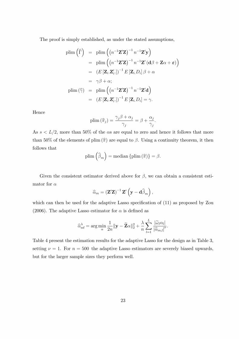
Table 4 present the estimation results for the adaptive Lasso for the design as in Table 3,
setting ν = 1. For n = 500 the adaptive Lasso estimators are severely biased upwards,
but for the larger sample sizes they perform well.
23
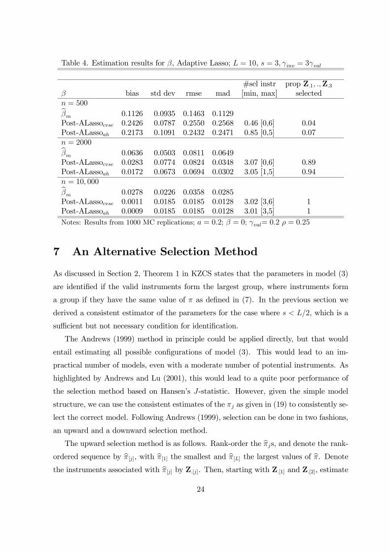
Table 4. Estimation results for β, Adaptive Lasso; L = 10, s = 3, γinv = 3γval
#sel instr prop Z.1, .,Z.3
β bias std dev rmse mad [min, max] selectedn = 500
βm 0.1126 0.0935 0.1463 0.1129Post-ALassocvse 0.2426 0.0787 0.2550 0.2568 0.46 [0,6] 0.04Post-ALassoah 0.2173 0.1091 0.2432 0.2471 0.85 [0,5] 0.07n = 2000
βm 0.0636 0.0503 0.0811 0.0649Post-ALassocvse 0.0283 0.0774 0.0824 0.0348 3.07 [0,6] 0.89Post-ALassoah 0.0172 0.0673 0.0694 0.0302 3.05 [1,5] 0.94n = 10, 000
βm 0.0278 0.0226 0.0358 0.0285Post-ALassocvse 0.0011 0.0185 0.0185 0.0128 3.02 [3,6] 1Post-ALassoah 0.0009 0.0185 0.0185 0.0128 3.01 [3,5] 1Notes: Results from 1000 MC replications; a = 0.2; β = 0; γval= 0.2 ρ = 0.25
7 An Alternative Selection Method
As discussed in Section 2, Theorem 1 in KZCS states that the parameters in model (3)
are identified if the valid instruments form the largest group, where instruments form
a group if they have the same value of π as defined in (7). In the previous section we
derived a consistent estimator of the parameters for the case where s < L/2, which is a
suffi cient but not necessary condition for identification.
The Andrews (1999) method in principle could be applied directly, but that would
entail estimating all possible configurations of model (3). This would lead to an im-
practical number of models, even with a moderate number of potential instruments. As
highlighted by Andrews and Lu (2001), this would lead to a quite poor performance of
the selection method based on Hansen’s J-statistic. However, given the simple model
structure, we can use the consistent estimates of the πj as given in (19) to consistently se-
lect the correct model. Following Andrews (1999), selection can be done in two fashions,
an upward and a downward selection method.
The upward selection method is as follows. Rank-order the πjs, and denote the rank-
ordered sequence by π[j], with π[1] the smallest and π[L] the largest values of π. Denote
the instruments associated with π[j] by Z.[j]. Then, starting with Z.[1] and Z.[2], estimate
24

model (3) by two-step GMM treating Z.[1] and Z.[2] as the valid instruments and compute
Hansen’s J-statistic. Using the same setup as in Section 3, Z.[1] and Z.[2] form a group
of instruments if the J-test is smaller than the corresponding critical value ζn,1. If that
is the case, we then add in subsequent steps Z.[3],Z.[4]... until the Hansen J-test rejects.
If this happens at the l-th step, thenZ.[1], ...,Z.[l−1]
forms a group of instruments. We
then repeat this sequence starting with Z.[2] and Z.[3], until the last pair Z.[L−1] and Z.[L]
has been evaluated. We then select as the valid instruments the group with the largest
number of instruments, or, as in Andrews (1999), if there are multiple groups with the
largest number of instruments, we select within this set the one with the smallest value
of the J-test. If there are no groups of size two and above, then none of the instruments
can be classified as valid.
The downward selection method is similar, but starts from the model with the set of
valid instruments being all instruments,Z.[1], ...,Z.[L]
. If this model is rejected, con-
sider the setZ.[1], ...,Z.[L−1]
etc. until the Hansen J−test does not reject, or the set
Z.[1],Z.[2]
has been evaluated. Then repeat the procedure starting from
Z.[2], ...,Z.[L]
,
until the final setZ.[L−1],Z.[L]
has been reached. The final model selection is as de-
scribed above for the upward testing procedure. Clearly, for both procedures models with
a smaller number of valid instruments than the largest group already identified need not
be evaluated.
Under the assumption that the group of valid instruments is the largest group, and
for the critical values of the J-test obeying assumptions (14) as in Andrews (1999), these
procedure will consistently select the correct model. Table 5 presents results for the
2SLS estimator after applying the upward selection method for the same design as in
Tables 1/2 and 3/4. The results of the downward procedure are virtually identical. It
is clear that for these designs, this sequential approach performs very similar to the best
performing (adaptive) post-Lasso estimators.
25

Table 5. Estimation results for β, Upward selection procedure; L = 10, s = 3
2SLSah,up #sel instr prop Z.1, .,Z.3
β bias std dev rmse mad [min, max] selectedγinv = γvaln = 500 0.0568 0.1230 0.1354 0.0816 2.50 [0,4] 0.54n = 2000 0.0043 0.0426 0.0428 0.0285 3.01 [3,5] 1n = 10, 000 0.0006 0.0183 0.0183 0.0127 3.01 [3,4] 1γinv = 3γvaln = 500 0.2396 0.1034 0.2610 0.2616 0.81 [0,4] 0.05n = 2000 0.0161 0.0751 0.0768 0.0285 2.97 [1,4] 0.94n = 10, 000 0.0006 0.0184 0.0184 0.0127 3.01 [3,4] 1Notes: Results from 1000 MC replications; a = 0.2; β = 0; γval= 0.2 ρ = 0.25
Again, for n = 500, the method produces a substantially upward biased estimator
when γinv = 3γval. This behaviour can be understood as follows. As
Yi = Diβ + Z′i.α + εi = Z′i. (γβ + α) + εi + viβ
= Z′i.Γ + εi + viβ,
we have for this particular design that, under standard regularity conditions, the limiting
distribution of Γ is given by
√n(
Γ− Γ)
d→ N (0, I) .
As
π = T−1γ Γ
where Tγ = diag(γj), i.e. a diagonal matrix with diagonal elements
γj, it follows that
√n (π − π)
d→ N(0, T−2γ
),
or
πa∼ N
(π, n−1T−2γ
). (21)
Using this asymptotic distribution to approximate the finite sample distribution, when
a = 0.2 and γinv = γval = 0.2, we have that a/γinv = 1, and for a valid and an invalid
instrument, we have
P (πval < πinv) = P
(πval − πinv + 1
2 (0.2√n)−1 <
1
2 (0.2√n)−1
)≈ Φ
(0.1√n),
26

which is equal to 0.987 for n = 500. When γinv = 3γval = 0.6, we have that a/γinv = 1/3,
and
P (πval < πinv) = P
(πval − πinv + 1/3
(0.2√n)−1
+ (0.6√n)−1 <
1/3
4 (0.6√n)−1
)≈ Φ
(0.05√n),
which is equal to 0.868 for n = 500. When taking 100, 000 draws from the distribution
(21) we find that when γinv = γval = 0.2, and n = 500, for 98.6% of the draws the
π[L−2], ...πL are those associated with the 3 invalid instruments, i.e. with those that have
nonzero α. When γinv = 3γval = 0.6, this percentage drops to 43.4%. So we see that the
relative strength of the invalid instruments affects the ability to segregate the valid and
invalid instruments by the values of π in finite samples.
8 An application, the effect of BMI on school out-comes using genetic markers as instruments
We have data on 111, 091 individuals from the UK Biobank and investigate the effect
of BMI on school outcomes. We use 95 genetic markers as instruments for BMI as
identified in independent GWAS studies. The linear model specification includes age,
age2 and sex, together with 15 principal components of the genetic relatedness matrix as
additional explanatory variables. Table 6 presents the estimation results for the causal
effect parameter of BMI. As critical value for the test based procedures we take again
0.1/ ln (n) = 0.0086.
27

Table 6. Estimation resultsestimate st err # sel instr p-value J-test j : Z.j selected
OLS -0.300 0.0122SLS -0.203 0.083 0 0.0008
Lassocv -0.206 19Post-Lassocv -0.323 0.105 19 0.9945Post-Lassocvse -0.203 0.083 0 0.0008Post-Lassobcch -0.203 0.083 0 0.0008Post-Lassoah -0.136 0.084 2 0.0316 78, 86ALassocvse -0.193 3
Post-ALassocvse -0.172 0.085 3 0.0894 5, 78, 86Post-ALassoah -0.204 0.084 2 0.0272 5, 86
2SLSah,up -0.168 0.083 4 0.0107 32, 38, 51, 862SLSah,down -0.161 0.083 2 0.0097 51, 86
Note: Coeffi cients and standard errors multiplied by 10.
The J-test rejects the model treating all 95 instruments as valid, but from the various
selection methods, we find that selecting 2 instruments as invalid is suffi cient for the J-
test to not reject the null of valid instruments. The Post-Lassoah, Post-ALassoah and the
2SLSah,down estimators all find 2 instruments as invalid, with the Post-Lassoah estimator
having the smallest value of the J-test. The Lassocv procedure selects too many, 19,
instruments as invalid, whereas both the Lassocvse and Lassobcch procedures don’t select
any instruments as invalid.
All selection procedures that do select instruments as invalid select instrument number
86. This is rs1808579_CT. The Post-Lassoah estimator further selects rs3888190_CA,
whereas the Post-ALassoah procedure selects rs3101336_TC instead. Interestingly, the
ALassocvse selects the union of these two sets of instruments, which is the third step
in the LARS algorithm for both the Lasso and adaptive Lasso procedures. Multiplying
the estimates by 10 for ease of exposition, we see that the potentially confounded OLS
estimate is equal to −0.30 (se 0.012), whereas the 2SLS estimate treating all instruments
as valid is smaller and equal to −0.20 (se 0.083). The Post-Lassoah estimate is equal to
−0.14 (se 0.084), whereas the the Post-ALassoah estimate is equal to −0.20 (se 0.084)
and that of the Post-ALassocvse estimator is equal to −0.172 (se 0.085). So we see that
there is considerable heterogeneity in the results, although these are all pointing to a
smaller effect than the observational one. This is also the case for the 2SLSah,down and
2SLSah,up results of −0.161 (se 0.083) and −0.168 (se 0.083) respectively.
28

References
[1] Andrews, D.W.K., (1999), Consistent Moment Selection Procedures for Generalized
Method of Moments Estimation, Econometrica 67, 543-564.
[2] Angrist, J.D., and A.B. Krueger (1991), Does Compulsory School Attendance Affect
Schooling and Earnings?, Quarterly Journal of Economics 106, 979-1014.
[3] Belloni, A., D. Chen, V. Chernozhukov and C. Hansen, (2012), Sparse Models and
Methods for Optimal Instruments with an Application to Eminent Domain, Econo-
metrica 80, 2369-2429.
[4] Bowden, J., G.D. Smith, S. Burgess, (2015), Mendelian Randomization with In-
valid Instruments: Effect Estimation and Bias Detection through Egger Regression,
International Journal of Epidemiology 44, 512-525.
[5] Burgess, S., D.S. Small and S.G. Thompson, A Review of Instrumental Variable
Estimators for Mendelian Randomization, Statistical Methods in Medical Research,
in Press.
[6] Cheng, X., Z. Liao, (2015), Select the Valid and Relevant Moments: An Information-
based LASSO for GMMwith ManyMoments, Journal of Econometrics 186, 443-464.
[7] Clarke, P.S. and F. Windmeijer, (2012), Instrumental Variable Estimators for Binary
Outcomes, Journal of the American Statistical Association 107, 1638-1652.
[8] Efron, B., T. Hastie, I. Johnstone and R. Tibshirani, (2004), Least Angle Regression,
The Annals of Statistics 32, 407-451.
[9] Greenland, S., (2000), An introduction to instrumental variables for epidemiologists,
International Journal of Epidemiology 29, 722-729.
[10] Han, C., (2008), Detecting Invalid Instruments using L1-GMM, Economics Letters
101, 285-287.
[11] Hansen, L.P., (1982), Large Sample Properties of Generalized Method of Moments
Estimators, Econometrica 50, 1029-1054.
29
[12] Imbens, G.W., (2014), Instrumental Variables: An Econometrician’s Perspective,
NBER Working Paper 19983.
[13] Jing, B.-Y., Q.-M. Shao and Q. Wang, (2003), Self-Normalized Cramér-Type Large
Deviations for Independent Random Variables, The Annals of Probability 31, 2167-
2215.
[14] Kang, H., A. Zhang, T.T. Cai and D.S. Small, (2015), Instrumental Variables Esti-
mation with some Invalid Instruments and its Application to Mendelian Random-
ization, Journal of the American Statistical Association, in Press.
[15] Kolesar, M., R. Chetty, J. Friedman, E. Glaeser, G.W. Imbens, (2015), Identification
and Inference with Many Invalid Instruments, Journal of Business and Economic
Statistics, in press.
[16] Lawlor, D.A., R.M. Harbord, J.A.C. Sterne,N. Timpson and G. Davey Smith, (2008),
Mendelian Randomization: Using Genes as Instruments for Making Causal Infer-
ences in Epidemiology, Statistics in Medicine 27, 1133-1163.
[17] Liao, Z., (2013), Adaptive GMM Shrinkage Estimation with Consistent Moment
Selection, Econometric Theory 29, 857-904.
[18] Lin, W., R. Feng, H. Li, (2015), Regularization Methods for High-Dimensional In-
strumental Variables Regression With an Application to Genetical Genomics, Jour-
nal of the American Statistical Association 110, 270-288.
[19] Sargan, J. D., (1958), The Estimation of Economic Relationships Using Instrumental
Variables. Econometrica 26, 393—415.
[20] Staiger, D. and J.H. Stock, (1997), Instrumental Variables Regression with Weak
Instruments, Econometrica 65, 557-586.
[21] Stock, J.H. and M. Yogo, (2005), Testing for weak instruments in linear IV regres-
sion. In D.W.K. Andrews and J.H. Stock (Eds.), Identification and Inference for
Econometric Models, Essays in Honor of Thomas Rothenberg, 80-108. New York:
Cambridge University Press.
30
[22] Zou, H., (2006), The Adaptive Lasso and Its Oracle Properties, Journal of the
American Statistical Association 101, 1418-1429.
9 Appendix
9.1 LARS
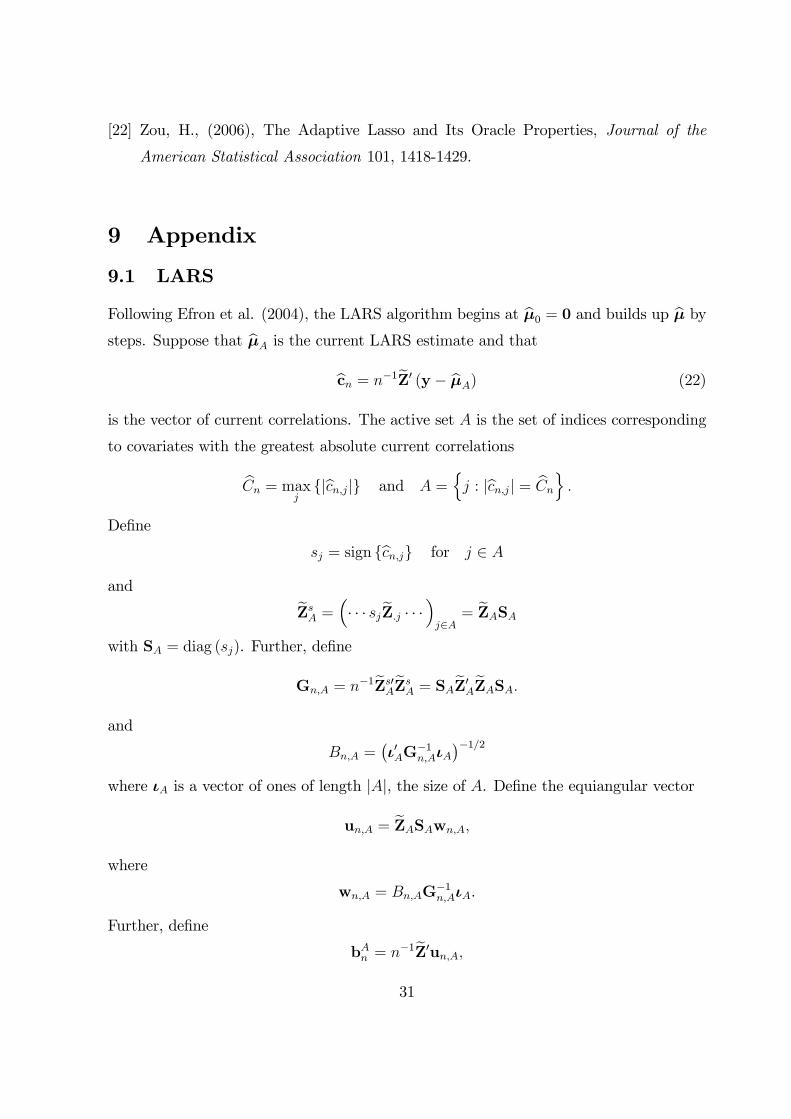
Following Efron et al. (2004), the LARS algorithm begins at µ0 = 0 and builds up µ by
steps. Suppose that µA is the current LARS estimate and that
cn = n−1Z′ (y − µA) (22)
is the vector of current correlations. The active set A is the set of indices corresponding
to covariates with the greatest absolute current correlations
Cn = maxj|cn,j| and A =
j : |cn,j| = Cn
.
Define
sj = sign cn,j for j ∈ A
and
ZsA =
(· · · sjZ.j · · ·
)j∈A
= ZASA
with SA = diag (sj). Further, define
Gn,A = n−1Zs′AZs
A = SAZ′AZASA.
and
Bn,A =(ι′AG−1n,AιA
)−1/2where ιA is a vector of ones of length |A|, the size of A. Define the equiangular vector
un,A = ZASAwn,A,
where
wn,A = Bn,AG−1n,AιA.
Further, define
bAn = n−1Z′un,A,
31

with j-th element bAn,,j.
Then the next step of the LARS algorithm updates µA to
µA+ = µA + κAun,A
where
κA = minj∈Ac
+
Cn − cn,jBn,A − bAn,j
,Cn + cn,jBn,A + bAn,j
(23)
where min + indicates that the minimum is taken over only positive components within
each choice of j. κA is the smallest positive value of κA such some new index j joins the
active set; j is the minimizing index in (23) and the new active set A+ is A ∪j. The
updated correlations are equal to cn,j − κAbAn,j, the new maximum absolute correlation isCn,+ = Cn − κABn,A, which is the value of the correlations for the active set A+.
Assuming that all γjs are the same and that E [Zi.Z′i.] = plim (n−1Z′Z) = IL, we have
that
plim(n−1Z′Z
)= I− L−1ιLι′L,
and hence
plim(Ωn
)= diag
(√1− L−1
)and so we can ignore Ω asymptotically for this case and focus on cn as defined above in
(22).
As
plim(n−1Z′AZA
)= IA − L−1ιAι′A,
it follows that
GA = plim(n−1Gn,A
)= S′A
(IA − L−1ιAι′A
)SA
= IA − L−1sAs′A,
where sA is the |A| vector of signs sj. Hence,
G−1A = IA + (L− |A|)−1 sAs′A
and
BA = plim (Bn,A) =(ι′AG−1A ιA
)−1/2=(|A|+ (L− |A|)−1 q2A
)−1/232

where
qA = ι′AsA
is the difference in the numbers of +1 and −1 in sA. Further,
wA = plim (wn,A) = BAG−1A ιA = BA
(ιA +
qA(L− |A|)sA
)and
plim(n−1SAZ′AuA
)= BAιA.
Then
bA = plim(bAn)
=
plim(n−1Z ′AZASAwA
)plim
(n−1Z ′AcZASAwA
) =
[(IA−L−1ιAι′A) SAwA
−L−1ιAcι′ASAwA
]
Consider the case as described in Section 2 with all non-zero αs being positive, and
ordered such that α1 > α2 > .. > αs > αs+1 = ... = αL = 0. We have at µ0 = 0,
plim (cn) = plim(n−1Z′y
)= α− α. (24)
It follows that if (α1 − α) > α, then A = A1 = 1 and C = |α1 − α|. The minimum κA1
for the invalid instruments is given by
min (κA1,inv) =(α1 − α)− (α2 − α)
BA1 − bA12=
α1 − α2BA1 − bA12
and for the valid instruments,
min (κA1,val) =(α1 − α) + (−α)
BA1 + bA1val=
α1 − 2α
BA1 + bA1val
and so the invalid Z.2 enters the active set if
α1 − α2BA1 − bA12
<α1 − 2α
BA1 + bA1val,
and then κA1 = min (κA1,inv).
At step m, assume that m < s invalid instruments have been selected, hence A =
Am = 1, 2, ...,m. For all A1...Am we have that all correlations are positive, so SA = IA,
sA = ιA, qA = |A|, and
BA =
(L− |A|L |A|
)1/233

wA = BA
(1 +
|A|L− |A|
)ιA = BA
(L
L− |A|
)ιA
bAjj+1 = b
Ajval = −BAj
(|Aj|
L− |Aj|
).
As there are no Lasso steps, |Aj| = j.
By repeated substitution, the minimum κAm for the invalid instruments is then given
by
min κAm,inv =
(α1 − α−
∑m−1j=1 κAjBAj
)−(αm+1 − α−
∑m−1j=1 κAjb
Ajm+1
)BAm − bAmm+1
=α1 − αm+1 −
∑m−1j=1 (αj − αj+1)
BAm − bAmm+1=
αm − αm+1BAm − bAmm+1
.
For the valid instruments it is given by
min κAm,val =
(α1 − α−
∑m−1j=1 κAjBAj
)+(−α−
∑m−1j=1 κAjb
Ajval
)BAm + bAmval
=
α1 − 2α−∑m−1
j=1 (αj − αj+1)BAj+b
Ajval
BAj−bAjj+1
BAm + bAmvalas
BAj + bAjval = BAj
(1− |Aj|
L− |Aj|
)= BAj
(L− 2 |Aj|L− |Aj|
)and
BAj − bAjj+1 = BAj
(1 +
|Aj|L− |Aj|
)= BAj
(L
L− |Aj|
)it follows that
BAj + bAjval
BAj − bAjj+1
=L− 2 |Aj|
L=L− 2j
L.
Therefore
α1 − 2α−m−1∑j=1
(αj − αj+1)BAj + b
Ajval
BAj − bAjj+1
= α1 − 2α−m−1∑j=1
(αj − αj+1)L− 2j
L
=L− 2 (m− 1)
L
(αm − 2α(m−1)
L− (m− 1)
L− 2 (m− 1)
)34

where
α(m−1) =1
L− (m− 1)
L∑j=m
αj.
Then the next invalid instrument gets selected if
αm − αm+1BAm − bAmm+1
<
L−2(m−1)L
(αm − 2α(m−1)
L−(m−1)L−2(m−1)
)BAm + bAmval
αm − αm+1 <L− 2 (m− 1)
L
(αm − 2α(m−1)
L− (m− 1)
L− 2 (m− 1)
)(L
L− 2m
)αm+1 > 2α(m)
L−mL− 2m
.
Hence the LARS algorithm selects the last invalid instrument at step s if
αs > 2α(s−1)L− (s− 1)
L− 2 (s− 1)= 2
αsL− (s− 1)
L− (s− 1)
L− 2 (s− 1)
L− 2s+ 2 > 2 ⇔ s < L/2.
For L even, if s = L/2 thenmin (κAs,inv) = min (κAs,val) and all remaining instruments
get in principle selected as invalid. In practice therefore, the invalid instrument may or
may not be selected as invalid. If s > L/2, the valid instruments get selected as invalid
before all invalid ones have been selected, and hence there is no path that includes all
invalid instruments.
35