2/13/2010

1

Survival Analysis Using SAS Proc LifetestSAS Proc Lifetest

Proc Lifetest

Estimation of Survival Probabilities Confidence Intervals and Bands,mean life, median life

B i PlBasic PlotsEstimates of Hazards, log survival, etc.Basic plots

Tests of equality of groups

Sample Data

866 AML or ALL patientsMain Effect is Conditioning Regimen

71 (52 Dead) Regimp=1 (non-myeloablative)171 (93 D d ) R i 2 ( d d i i171 (93 Dead ) Regimp=2 (reduced intensity625 (338 Dead) Regimp=4 (myeloablative)

Other Variables

sex patient's gender 1 (male), 2 (female)

disease 10 (AML), 20 (MDS)

agedec age by decade3 (30-39), 4 (40-49),5 (50-59)

graftype 1 (BM), 2 (PB)

kps0 (<90), 1 (>90),99 (unknown)

danhlagrp2 type of donor0 (HLA-matched sibs), 1 (well-matched URD)

yeartx year of transplant2000, 2001, 2002, 2003, 2004

Outcome Variables

Overall Survivalintxsurv – time from BMT to death or end of studydead – 1 dead 0 alive

R l /TRM i blRelapse/TRM variablesinterval– time from BMT to death or relapsetrm – 1 if dead in remission, 0 otherwiserel – 1 if relapse prior to death, 0 otherwiselfs = trm+rel – 1 if dead or relapsed, 0 otherwise

Two Kinds of Outcomes

Survival OutcomesObserve T = min(Event time, censoring time) d=event indicator

1 event1 event 0 censored observation Censoring times are independent of event times

Example: Overall Survival, Disease Free SurvivalSummary Statistics: Survival function, hazard rate, mean/median time to event

2/13/2010

2

Two Kinds of Outcomes

Competing Risk DataTwo events e.g.. Relapse, DeathOccurrence of one of the events precludes occurrence of the other

i (Ti 1 Ti 2)X=min(Time to event 1, Time to event 2)T=min(X, time to censoring)Two event indicators R=1 if event of type 1, 0 OW D=1 if event of type 2, 0 OW

Summary Statistics: Two cumulative incidence functions, crude hazard rate

Two Kinds of OutcomesCompeting Risk DATA

Examples

Event 1 Event 2 Censoring

Relapse Death in Remission Lost to follow-up

GVHD Death w/o GVHD 2nd transplant, lost to (Relapse w/o GVHD) follow-up

Engraftment (neurophil recovery)

Death w/o recovery2nd transplant prior to recovery

Lost to follow-up

Summary Statistics for Survival Data

X event timeSurvival function S(x)=P[X>x]

Hazard Rate

Note h(x)δx ≈ probability a patient alive at start of day x dies on x

h(x)=-d ln(S(x))/dx

0( ) lim [ | ]

xh x P x X x x X x

δδ

→= ≤ ≤ + ≥

Survival DataParameters

Cumulative Hazard RateH(x)= -ln[S(x)] = area under hazard rate curve up to x

Mean Survival Time d i lμ = area under survival curvepth Quantile

S(tp)=1-p

Summary Survival Estimates Using Proc Lifetest

• Proc Lifetest options;– Time statement– Strata statement

T t t t m nt ( phr )– Test statement (use phreg)– By statement– Freq statement– ID statement

Example Program 1

Data in Sas Data Set “study”

data nmb; set study;if regimp=1;

proc lifetest data=nmb;time intxsurv*dead(0);

2/13/2010

3

Standard Number NumberINTXSURV Survival Failure Error Failed Left 0.0000 1.0000 0 0 0 71 0.6908 0.9859 0.0141 0.0140 1 70 1.0526 0.9718 0.0282 0.0196 2 69 1.0855 0.9577 0.0423 0.0239 3 68 1.4803 0.9437 0.0563 0.0274 4 67 1.6118 . . . 5 66 1.6118 0.9155 0.0845 0.0330 6 65 2.4013 . . . 7 64

.

.

39.4079 0.2843 0.7157 0.0572 49 12 40.6908* . . . 49 11 45 7895 0 2585 0 7415 0 0576 50 1045.7895 0.2585 0.7415 0.0576 50 10 48.5855* . . . 50 9 49.3421* . . . 50 8 53.0921 0.2262 0.7738 0.0588 51 7 54.9342* . . . 51 6 62.2368* . . . 51 5 64.1447* . . . 51 4 70.6908* . . . 51 376.3816* . . . 51 2 86.1513* . . . 51 1 88.6184* . . . 51 0 NOTE: The marked survival times are censored observations.

Quartile Estimates

Point 95% Confidence IntervalPercent Estimate Transform[Lower Upper)75 53.0921 LOGLOG 31.9408 . 50 12.6974 LOGLOG 6.6118 27.203925 4.8355 LOGLOG 3.0263 6.1842

Mean Standard Error22.7630 2.5308

NOTE: The mean survival time and its standard error were underestimated because to the largest event time was censored and estimation was restricted to the largest on study time.

Summary of the Number of Censored and Uncensored Values

PercentTotal Failed Censored Censored

71 51 20 28.17

“Survival” Column is Kaplan-Meier Product-Limit estimator (KME)

“Standard Error” –Greenwood’s estimator of standard deviation of Kaplan-Meier estimatorMean is really the restricted mean.

Here the area under the KME up to the largest eventHere the area under the KME up to the largest event time (at 53.0921). Some programs compute area up to largest on study time (Here 88.6184). Limit can be changed to tmax by using proc lifetest timelim=tmax

Confidence Bands and Intervals95% Confidence interval for S(to)—95% sure true unknown survival function at time to is in the random interval SL(t o) to SU(t o)

95% Confidence band for S(t) over range[τ1,τ2] −− 95% sure true unknown survival function is

between the random curves SL(t ), SU(t ) for all τ1<t<τ2L( ) U( ) 1 2

Note Confidence bands much wider than confidence intervals

Confidence intervals/bands found by finding a confidence interval for g(S) and converting back to S

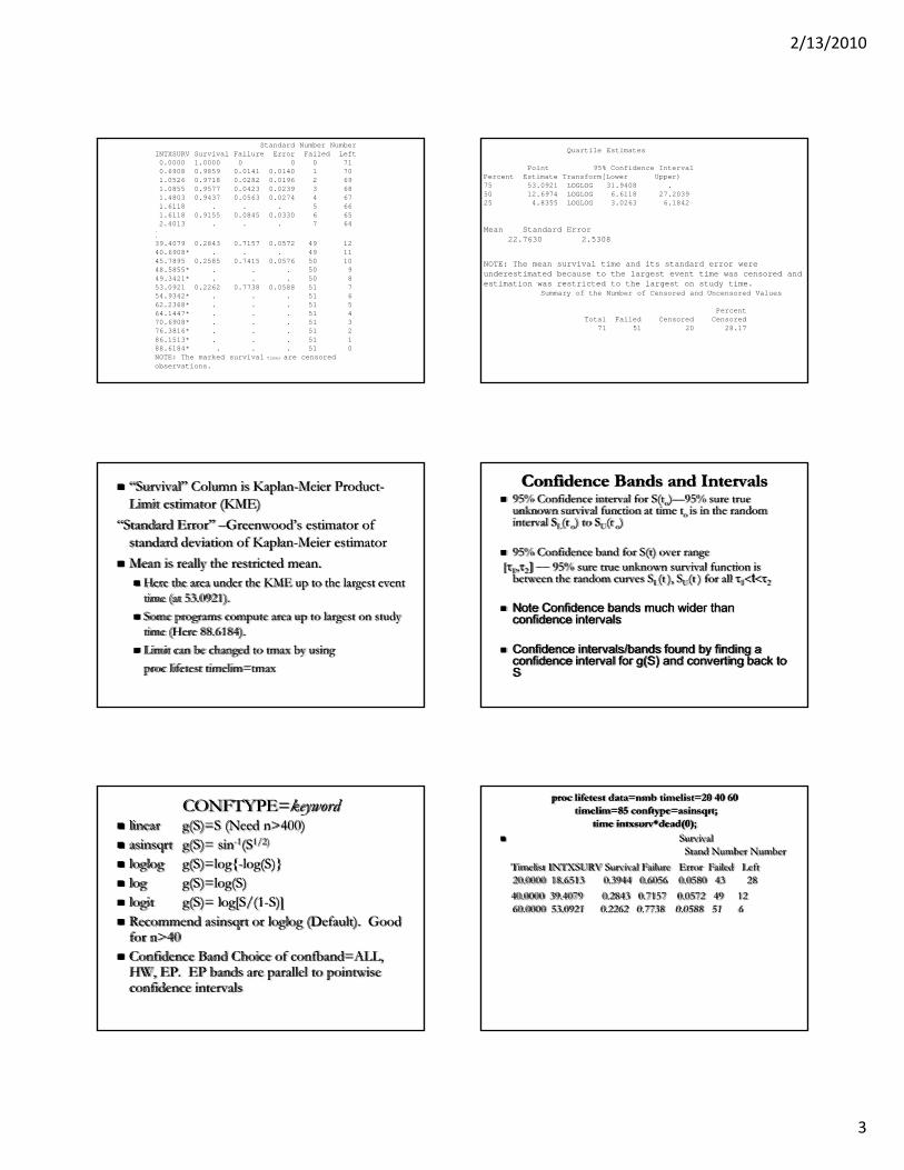
CONFTYPE=keywordlinear g(S)=S (Need n>400)asinsqrt g(S)= sin-1(S1/2)

loglog g(S)=log{-log(S)}log g(S)=log(S)logit g(S)= log[S/(1-S)]g g( ) g[ ( )]Recommend asinsqrt or loglog (Default). Good for n>40Confidence Band Choice of confband=ALL, HW, EP. EP bands are parallel to pointwise confidence intervals

proc lifetest data=nmb timelist=20 40 60timelim=85 conftype=asinsqrt;

time intxsurv*dead(0);Survival

Stand Number NumberTimelist INTXSURV Survival Failure Error Failed Left 20.0000 18.6513 0.3944 0.6056 0.0580 43 28 40.0000 39.4079 0.2843 0.7157 0.0572 49 12 60 0000 53 0921 0 2262 0 7738 0 0588 51 660.0000 53.0921 0.2262 0.7738 0.0588 51 6

2/13/2010

4

proc lifetest data=nmb timelist=20 40 60timelim=85 conftype=asinsqrt;

time intxsurv*dead(0);Quartile EstimatesPoint 95% Confidence Interval

Percent Estimate Transform [Lower Upper)75 53.0921 ASINSQRT 31.9408 . 50 12.6974 ASINSQRT 6.8092 27.203925 4.8355 ASINSQRT 3.4868 6.414525 4.8355 ASINSQRT 3.4868 6.4145

Mean Standard Error29.9793 4.0896NOTE: The mean survival time and its standard error were underestimated because the largest observation was censored and the estimation was restricted to a time less than the largest observation.

Output Data Set with Estimates

proc lifetest data=nmb notable outsurv=survest conftype=asinsqrt confband=ep bandmintime=10 bandmaxtime=70 timelist =5 10 20 30 40 50 60 70 80 reduceouttimelist 5 10 20 30 40 50 60 70 80 reduceout noprint stderr ;time intxsurv*dead(0);

proc print data=survest;

SDF_Obs TIMELIST INTXSURV _CENSOR_ SURVIVAL STDERR 1 5 4.9671 0 0.73239 0.052540 2 10 8.8487 0 0.52113 0.059286 3 20 18.6513 0 0.39437 0.0580004 30 27.2039 0 0.37920 0.057718 5 40 39.4079 0 0.28431 0.057243 6 50 45.7895 0 0.25847 0.057579 7 60 53.0921 0 0.22616 0.058751 8 70 53.0921 0 0.22616 0.058751 9 80 53 0921 0 0 22616 0 0587519 80 53.0921 0 0.22616 0.058751 Obs SDF_LCL SDF_UCL EP_LCL EP_UCL1 0.62409 0.82819 . . 2 0.40540 0.63571 . . 3 0.28456 0.50987 0.24365 0.556184 0.27036 0.49457 0.23008 0.541065 0.17991 0.40199 0.14341 0.451086 0.15484 0.37806 0.11950 0.428527 0.12277 0.35017 0.08905 0.403398 0.12277 0.35017 0.08905 0.403399 0.12277 0.35017 0.08905 0.40339

Graphs Using ODS graphics

Decide on output file type (pdf, html, rtf)ods pdf file=‘ex1.pdf’;

Enable ods graphicsods graphics on;ods graphics on;

Lifetest code with plot requests in plots=(list) optionsProc lifetest plots=(survival); Time t*d(1,2); run;

Turn ODS graphics offOds graphics off

Basic Graphs

ods pdf file=‘ex1.pdf’;ods graphics on;proc lifetest data=study plots=(survival, lls, ls);time intxsurv*dead(0);strata regimp;run;ods graphics off;

2/13/2010

5

plots=(ls)vertical: cumulative hazard horizontal: time

Cox model suggests curves should be multiples of each otherH1(t)=θ1H2(t)

plots=(lls)vertical: log cumulative hazard horizontal:log time

Cox model suggests curves should be parallellog(H1(t)) =log(θ1)+log(H2(t))

ods pdf file=‘ex1.pdf’;ods graphics on;proc lifetest data=study

plots=(survival (atrisk=0 to 80 by 20 nocensor failure));time intxsurv*dead(0); strata regimp; run;

ods graphics off;

ods pdf file=‘ex1.pdf’;ods graphics on;proc lifetest data=study

plots=(survival (cl cb=ep strata=panel));time intxsurv*dead(0); strata regimp; run;

ods graphics off;

ods pdf file=‘ex1.pdf’;ods graphics on;proc lifetest data=study plots=(hazard(bw=10));

time intxsurv*dead(0); strata regimp; run;ods graphics off;

Summarizing Competing Risks

X time to smaller of two risksEvent indicators

R=1 if event of type 1, 0 owD=1 if event of type 2, 0 ow ε=1 if type 1 event, 2 if type 2 event 0 ow

Crude Hazard Rates

h1(x)dx ≈ Chance a patient will experience a type 1 event today given they have not experienced either event at the start of the day

1 0( ) lim [ , 1| ]

xh x P x X x x X x

δδ ε

→= ≤ ≤ + = ≥

2/13/2010

6

Summarizing Competing Risks

Cumulative Incidence Function

1

1 1 200

( ) [ , 1]

( ) exp [ [ ( ) ( ) ] ]t

u

C t P X t

h u h v h v d v du

ε= ≤ =

= − +∫ ∫

NOTES:Proc Lifetest does not provide estimates of these quantitiesProc Lifetest can be used for tests for competing risksSAS macros available to compute cumulative incidence

0

Cumulative incidence macrohttp://www.mcw.edu/FileLibrary/Groups/Biostatistics/Software/SAS_

Macro_For_Cumulative_Incidence_Functions.txt

Download macro to your working directoryAssuming macro is in file cimacro in your home directory use%include ‘cimacro’ ;%include cimacro ;Use %incid(data,group,event1,event2,time,out=outdsn);

data—name if data set where your data isgroup--- variable with group indicatorsevent1, event 2—event indicators, outdsn – data set name of an output data set if desired

Sample Programoptions linesize=80; libname in '';data study; set in.short_course;if trm=. then delete; if interval=. then delete;if regimp=4 then regimp=3;

%include ‘cimacro.txt';%incid(study,regimp,rel,trm,interval,out=in.outa);run;proc print;ods pdf file='ci.pdf';ods graphics on;title 'treatment related mortality';title treatment related mortality ;

symbol1 color=blue i=steplj v=none w=3 l=2 ;symbol2 color=red i=steplj v=none w=3 l=14;symbol3 color=green i=steplj v=none w=3 l=34;axis1 label=(c=black "Years") order=(0 to 80 by 10) ;axis2 label=(a=90 c=black "Cumulative incidence") order=(0 to 1 by .2);proc gplot;plot ci2*time=group /haxis=axis1 vaxis=axis2 overlay noframe;run;title 'relapse';proc gplot;plot ci1*time=group /haxis=axis1 vaxis=axis2 overlay noframe;run;ods graphics off;

Obs time group CI1 SE_CI1 CI2 SE_CI2

1 0.03000 1 0.000000 0.000000 0.000000 0.0000002 0.26316 1 0.000000 0.000000 0.000000 0.000000

15 0.69079 1 0.000000 0.000000 0.014706 0.01449016 0.72368 1 0.000000 0.000000 0.014706 0.014490

194 5.95400 1 0.29285 0.057851 0.13880 0.043037195 5.98684 1 0.29285 0.057851 0.13880 0.043037196 6.05300 1 0.29285 0.057851 0.13880 0.043037

1506 5.95400 3 0.13692 0.014124 0.20193 0.0164561507 5.98684 3 0.13692 0.014124 0.20362 0.0165141508 6.05300 3 0.13861 0.014203 0.20362 0.016514

1966 86.4145 3 0.27471 0.021835 0.33132 0.0215741967 86.5461 3 0.27471 0.021835 0.33132 0.0215741968 89.0461 3 0.27471 0.021835 0.33132 0.021574

2/13/2010

7

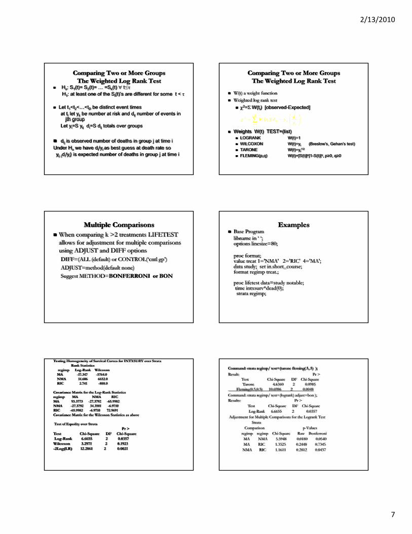
Comparing Two or More GroupsThe Weighted Log Rank Test

Ho: S1(t)= S2(t)= … =Sk(t) ∀ t≤τH1: at least one of the Si(t)’s are different for some t < τ

Let t1<t2<…<tD be distinct event timesat ti let yij be number at risk and dij number of events in

jth groupjth groupLet yi=S yij di=S dij totals over groups

dij is observed number of deaths in group j at time iUnder Ho we have di/yi as best guess at death rate soyij {di/yi} is expected number of deaths in group j at time i

Comparing Two or More GroupsThe Weighted Log Rank Test

W(t) a weight functionWeighted log rank test

χ2=Σ W(ti) [observed-Expected]

2 ( )[D

idW t d yχ⎛ ⎞⎜ ⎟∑

Weights W(t) TEST=(list)LOGRANK W(t)=1WILCOXON W(t)=yi (Breslow’s, Gehan’s test)TARONE W(t)=yi

1/2

FLEMING(p,q) W(t)=[S(t)]p[1-S(t)]q, p≥0, q≥0

1

( )[ ii ij ij

i i

W t d yy

χ=

= − ⎜ ⎟⎝ ⎠

∑

Multiple ComparisonsWhen comparing k >2 treatments LIFETEST allows for adjustment for multiple comparisons using ADJUST and DIFF optionsDIFF=(ALL (default) or CONTROL(‘cntl gp’)ADJUST= th d(d f lt )ADJUST=method(default none)Suggest METHOD=BONFERRONI or BON

ExamplesBase Programlibname in ‘ ‘;options linesize=80;

proc format;value treat 1='NMA' 2='RIC' 4='MA';data study; set in short course;data study; set in.short_course;format regimp treat.;

proc lifetest data=study notable;time intxsurv*dead(0);strata regimp;

Testing Homogeneity of Survival Curves for INTXSURV over StrataRank Statistics

regimp Log-Rank WilcoxonMA -17.347 -5764.0NMA 14.606 6652.0RIC 2.741 -888.0

Covariance Matrix for the Log-Rank Statisticsregimp MA NMA RICMA 93.3773 -27.3792 -65.9982NMA -27.3792 34.3501 -6.9710RIC -65.9982 -6.9710 72.9691Covariance Matrix for the Wilcoxon Statistics as aboveCovariance Matrix for the Wilcoxon Statistics as above

Test of Equality over Strata Pr >

Test Chi-Square DF Chi-Square Log-Rank 6.6655 2 0.0357 Wilcoxon 3.2971 2 0.1923 -2Log(LR) 12.2861 2 0.0021

Command: strata regimp/ test=(tarone fleming(.5,.5) );

Result: Pr > Test Chi-Square DF Chi-SquareTarone 4.6360 2 0.0985

Fleming(0.5,0.5) 10.6986 2 0.0048 Command: strata regimp/ test=(logrank) adjust=bon ); Results: Pr >

Test Chi-Square DF Chi-SquareLog-Rank 6.6655 2 0.0357

Adjustment for Multiple Comparisons for the Logrank TestStrata

Comparison p-Valuesregimp regimp Chi-Square Raw BonferroniMA NMA 5.5948 0.0180 0.0540MA RIC 1.3525 0.2448 0.7345NMA RIC 1.1611 0.2812 0.8437

2/13/2010

8

Command: test=(logrank) adjust=bon diff=control('MA') Result: Pr >

Test Chi-Square DF Chi-SquareLog-Rank 6.6655 2 0.0357

Adjustment for Multiple Comparisons for the Logrank TestStrata

Comparison p-Valuesregimp regimp Chi-Square Raw Bonferroni

NMA MA 5 5948 0 0180 0 0360NMA MA 5.5948 0.0180 0.0360RIC MA 1.3525 0.2448 0.4897

command strata yeartx/test=(logrank wilcoxon) trendScores for Trend Test

yeartx Score2000 20002001 20012002 20022003 20032004 2004

Trend Tests

Test StandardTest Statistic Error z-Score Pr > |z| Pr < z Pr > zLog-Rank 0.7428 30.5105 0.0243 0.9806 0.5097 0.4903Wilcoxon -12632.000 19140.7316 -0.6600 0.5093 0.2546 0.7454