Estimating the Global Investment Gap in Research and

Estimating the Global Investment Gap in Research and Innovation for Sustainable Agriculture Intensification in the Global South

Commission on Sustainable Agriculture Intensification

Estimating the global investment gap in research and innovation for sustainable agriculture intensification in the Global South

International Food Policy Research Institute

July 2021

ii

This study was carried out by the International Food Policy

Research Institute.

International Food Policy Research Institute. 2021. Estimating the global investment gap in research

and innovation for sustainable agriculture intensification in the Global South. Colombo, Sri Lanka:

Commission on Sustainable Agriculture Intensification. 65p.

Copyright © 2021, Commission on Sustainable Agriculture Intensification

Fair use:

Unless otherwise noted, you are free to copy, duplicate or reproduce, and distribute, display or

transmit any part of this report or portions thereof without permission, and to make translations,

adaptations or other derivative works under the following conditions:

ATTRIBUTION: The work must be referenced according to international standards, but not in

any way that suggests endorsement by WLE, IWMI or the author(s).

NON-COMMERCIAL: This work may not be used for commercial purposes.

SHARE ALIKE: If this work is altered, transformed or built upon, the resulting work must be

distributed only under the same or similar Creative Commons license to this one.

Disclaimer:

The opinions expressed in this paper and any possible errors are the responsibility of the authors. They

do not necessarily reflect the position of the Commission on Sustainable Agriculture Intensification,

the UK Foreign, Commonwealth & Development Office, or of the institutions and individuals who were

involved in the preparation of the report.

iii

Acknowledgements

CoSAI was initiated and is supported by the CGIAR Research Program on Water, Land and Ecosystems

(WLE), funded by the CGIAR Trust Fund and other donors. CoSAI Commissioners are independent.

CoSAI is facilitated by a Secretariat based at the International Water Management Institute (IWMI)

headquarters in Colombo, Sri Lanka.

Donors

The research was co-financed by the UK's Foreign, Commonwealth & Development Office (FCDO) and

CoSAI.

UK Government Foreign, Commonwealth and Development

Office (FCDO)

This research was carried out as part of the CGIAR Research

Program on Water, Land and Ecosystems (WLE) and

supported by Funders contributing to the CGIAR Trust Fund

(https://www.cgiar.org/funders/)

https://wle.cgiar.org/

https://www.cgiar.org/funders/

v

Contents

Executive summary ............................................................................................................................... vii

1 Introduction .................................................................................................................................... 1

2 Methodology ................................................................................................................................... 2

IMPACT global food model ................................................................................................................. 2

Investment scenarios .......................................................................................................................... 3

Technical mitigation options ............................................................................................................... 5

3 Results of investment scenarios by 2030 ........................................................................................ 6

An additional USD 2.1 billion per year in international public R&D above the reference scenario

counters the impact of climate change on hunger ............................................................................. 6

USD 4 billion per year in R&D brings the population at risk of hunger below 5% in most regions –

but not in SSA ...................................................................................................................................... 6

R&D investments bring down emissions by 402 MtCO₂eq in 2030 .................................................... 7

Another USD 6.5 billion per year in technical options is needed to deliver a mitigation trajectory .. 8

USD 4.7 billion per year in water resource management reduces blue water demand .................... 8

R&D investments and technical options substantially improve water quality ................................... 9

R&D and water investments generate USD 2 trillion per year in economic benefits to the Global

South ................................................................................................................................................... 9

R&D and investments reduce food prices by 16% ............................................................................ 10

4 Supporting policies and investments ............................................................................................ 11

5 Comparison with other studies ..................................................................................................... 12

6 Conclusion ..................................................................................................................................... 15

References ............................................................................................................................................ 17

Annex 1. Model and analysis ................................................................................................................ 27

The IMPACT model for investment scenario analysis ....................................................................... 27

Targets, trajectories and indicators for the analysis ......................................................................... 27

Annex 2. Scenarios and detailed results ............................................................................................... 30

Investment scenarios for agricultural R&D and water resource management ................................ 30

Hunger and economic outcomes ...................................................................................................... 33

GHG emission reductions through productivity growth ................................................................... 36

Technical options for climate change mitigation .............................................................................. 38

GHG emission reductions and sequestration through the adoption of technical options ............... 40

Water resources modeling and scenario costs ................................................................................. 43

Agricultural water pollution .............................................................................................................. 46

Limitations of the model and analysis .............................................................................................. 47

vi

Annex 3. Discussion of supporting policies and investments ............................................................... 50

Agricultural value chains ................................................................................................................... 50

Finance .............................................................................................................................................. 50

Extension ........................................................................................................................................... 51

Gender-responsive policies and investments ................................................................................... 51

Social protection ............................................................................................................................... 52

Water management .......................................................................................................................... 53

Carbon payments and smart subsidies ............................................................................................. 53

Agroecological and landscape approaches ....................................................................................... 54

Annex 4. Summary of key parameters in IMPACT ................................................................................ 56

vii

Executive summary

An investment gap stands in the way of sustainable agriculture intensification

Sustainable food production needs to increase if it is to meet the rising and evolving food demands

caused by growing populations, increasing incomes and urbanization. However, it faces numerous

challenges. Competition for water resources is increasing – not only between people and the natural

environment, but between cities and rural areas as well. Overuse of water due to wasteful irrigation

management is worsening water scarcity. Climate change is bringing higher temperatures and

changing precipitation patterns, as well as a higher likelihood of increased weather variability and

extreme events. At the same time, agriculture is a major contributor to greenhouse gas (GHG)

emissions, so sustainable agriculture intensification also needs to address climate change by reducing

GHG emissions and sequestering carbon.

These challenges can be addressed through investments in innovation for sustainable agriculture

intensification. Such investments in the Global South have the potential to achieve key ambitions of

the Sustainable Development Goals (SDGs) and the Paris Agreement on climate change. To do that,

however, an investment gap will have to be filled.

The investment gap is clear and measurable

This report estimates the size of the gap, and calculates the additional research and innovation

investments in the Global South that could bring hunger close to zero by 2030, in line with SDG2;

reduce GHG emissions from the agricultural sector, in line with SDG13 and consistent with a 2°C

climate trajectory; and improve efficiency of water use and reduce agricultural water pollution,

making progress toward SDG6.

Innovation for sustainable agriculture intensification is defined here as the creation, development and

implementation of new technologies, policies, techniques and management practices for sustainable

productivity growth, climate change mitigation and water resource improvement that drive progress

toward the SDG targets and 2°C climate trajectory.

The first part of this report uses an International Model for Policy Analysis of Agricultural Commodities

and Trade (IMPACT) scenario methodology to estimate the public and private investments in

agricultural research and development (R&D) that could reduce the share of population at risk of

hunger below 5% by 2030. This analysis measures the outcomes of these investments against a

reference scenario of business as usual that incorporates the impacts of climate change. In addition

to this modeling , an analysis of technical options for additional GHG mitigation draws on evidence in

the literature regarding potential impacts, costs and adoption rates of climate smart techniques and

management practices. We also model the investment in innovative water resource management that

will achieve substantial reductions in water use by 2030.

Investments can accelerate the end of hunger

Increased investments in agricultural R&D – by CGIAR, national agricultural research systems and the

private sector – would, together with investments that raise research efficiency, reach the SDG2

viii

hunger target in East Asia, South Asia and Latin American and the Caribbean. This is an impressive

achievement in the short time remaining until 2030. Sub-Saharan Africa would remain well above the

target with 11.8% at risk of hunger in 2030, although this is still a major improvement relative to the

24.3% share who were hungry in 2010. This investment scenario requires an additional USD 4 billion

per year above the reference scenario, an increase of 41% compared to the reference scenario

investments. The private sector would account for 13% of the additional investments.

These investments would adapt agriculture to climate change by erasing its effect on hunger seen in

the reference scenario. In fact, this adaptation is achieved by the USD 2.1 billion international public

component alone, which prevents climate change from pushing 66 million more people into risk of

hunger by 2030. By 2030, the investments would also raise incomes by 2% and gross domestic product

by USD 1.7 trillion in the Global South. They would also reduce global food prices by 16% and reduce

the degree of expansion of crop area harvested, thereby reducing GHG emissions relative to the

reference scenario.

Investments can make agriculture part of a 2°C climate trajectory

The assessment of technical mitigation options shows that much larger reductions in emissions can

be achieved in agriculture. By 2030, these have a mean non-CO2 mitigation potential equivalent to

715 million tons of CO2 per year, and a mean CO2 sequestration potential of 1,153 million tons per

year. The mean cost of generating these levels of technical mitigation is USD 6.5 billion per year in

2030, rising to USD 8.5 billion annually by 2050. Together with the emissions savings generated by

agricultural productivity growth, this technical mitigation helps the food system meet an emissions

trajectory by 2030 that is consistent with 2°C of warming. The combination of technical mitigation

expenditure and higher research expenditure does slow the expansion of land use driven by

agriculture over this period. But they are not, in themselves, sufficient to achieve zero land use change

induced by agriculture by 2050, which is critical if we are to achieve net zero, stabilizing global warming

at below 2°C.

Investments can rein in water use and pollution

Additional investments and improvements in agricultural water resource technology and

management for irrigated and rainfed areas would result in a 10% reduction in agricultural water use

in 2030 compared to the reference scenario. These include accelerated investments in modernization

of irrigation systems and water management for improved water use efficiency on irrigated cropland;

water conservation in rainfed areas through the implementation of rainwater harvesting, broad-beds

and furrows; and percolation dams and tanks and other technologies and management practices that

improve plant water uptake capacity and soil water holding capacity. These investments would need

to be targeted over large cropping areas and would require a combined increase in investment of USD

4.7 billion annually in the Global South. These increases are more than double (2.3 times) the annual

investments in the reference scenario.

Increased investment in agricultural R&D would also improve fertilizer use efficiency, and, together

with investment in technical options – precision agriculture techniques, integrated soil fertility

management, conservation tillage, and improved management of the nutrient cycle for recycling and

re-use in the livestock sector – would reduce non-point agricultural pollution from nitrogen in the

Global South by 21% in 2030 and 35% in 2050, relative to the reference scenario. Phosphorous

ix

pollution from agriculture is projected to decline by 14% in 2030 and by 15% in 2050 compared to the

reference scenario.

Now is the time to start closing the gap

To sum up the estimated investment gap, combining the agricultural R&D investments of USD 4 billion

per year required to nearly end hunger by 2030, and the investments of USD 6.5 billion per year in

technical climate smart options needed by 2030 to put the food system on an emissions trajectory

consistent with 2°C of global warming (although not achieving zero land use change from agriculture),

the innovation investment gap is USD 10.5 billion annually. Additional investments of USD 4.7 billion

in innovation for water use efficiency and water conservation would make substantial progress toward

the SDG6 water resource goals. Together these investments go a long way to meeting the targets, but

they are not fully sufficient. Supporting policies and investments are required in such areas as value

chains, finance, extension, gender-responsive policies and investments, social protection, water

management and the implementation of carbon payments and smart subsidies.

1

1. Introduction

If the world is to achieve the Sustainable Development Goals (SGDs), succeed in stabilizing global

warming at below 2°C, and adapt to the climate change this warming will bring, agricultural systems

must transform significantly by 2030. It will not be easy. A rising global population, rapid income

growth and urbanization are having profound effects on the demand and patterns of agricultural

production (Godfray et al. 2010; Hawkes et al. 2017; Rosegrant et al. 2017). While hunger persists for

too many people, diets continue to shift toward convenience foods and fast foods (Ruel et al. 2017;

Fan et al. 2019). There is increased consumption of fruits and vegetables; growing demand for sugar,

fats and oils; and rapid growth in meat consumption and therefore demand for feed grains or other

livestock feeds (Thornton 2010; Godfray et al. 2010; Kearney 2010; Rosegrant et al. 2017). As these

demands put pressure on food systems, sustainable food production growth also faces challenges

from climate change, with higher temperatures and changing precipitation patterns as well as a likely

increase in weather variability (Smith et al. 2018; Mbow et al. 2019).

At the same time, agriculture itself is a major contributor to greenhouse gas (GHG) emissions, so

sustainable intensification needs to contribute to climate change solutions by reducing GHG emissions

and sequestering carbon (Smith et al. 2018; Mbow et al. 2019). Agriculture needs to use less land if

the world is to reverse deforestation and halt the global collapse in biodiversity. And it needs to use

less water: amid rapidly growing demand (Damania et al. 2017), there must be a change in the

wasteful irrigation management that unnecessarily depletes groundwater around the world and

harms the quality of both agricultural and non-agricultural water supplies.

A transformation this large and rapid will require investment in innovations for sustainable agriculture

intensification. These are innovations that seek to produce the food needed to meet changing human

needs while simultaneously ensuring the long-term productive potential of natural resources, such as

water and land resources, and the associated ecosystems and their functions. This report aims to show

the size of that investment.

Specifically, this report aims to identify the innovation investment gap that needs to be filled to ensure

that sustainable agriculture intensification supports the achievement of specific global goals:

• Ensuring that less than 5% of the world’s population are at risk of hunger by 2030 (SDG2,

using the FAO threshold for zero hunger) (FAO et al. 2015).

• Reducing and sequestering emissions in agriculture, and stopping emissions from land use

change for food production, on a trajectory consistent with stabilizing climate below 2°C

(SDG13 and the Paris Agreement).

• Supporting adaptation of the agricultural system to a changing climate (SDG13 and the Paris

Agreement).

• Making substantial improvements in the efficiency of water use in agriculture (SDG6) and

reductions in agricultural water pollution (SDG6).

2

2. Methodology

For this study, innovation for sustainable agriculture intensification is defined as the creation,

development and implementation of new technologies, techniques and management practices for

sustainable productivity growth, climate mitigation and water resource improvement that drive

progress toward achieving the above goals and trajectories. The specific innovation investments that

are analyzed are:

• Public and private investments in agricultural research and development (R&D).

• Investments to support adoption of innovative technologies for climate change mitigation in

agriculture through carbon payments or other forms of targeted subsidies or payments of

environmental services (technical mitigation options).

• Investment in innovative management and technology for water use efficiency (WUE) and

soil water holding capacity (SWHC).

Analysis of the investment requirements and investment gap to 2030 used model-based investment

scenarios combined with analysis of specific climate smart and resource-saving technical options as

well as management practices that can reduce GHG emissions and increase GHG sequestration. SDG2

(zero hunger), SDG6 (clean water and sanitation), SDG13 (climate action) and the Paris Agreement on

climate change provide the specific sustainability context in which the investment gaps are evaluated;

the targets and indicators of progress used are detailed in Annex 1. The total investment gap includes

the required investment in agricultural R&D and the required investment in climate smart and

resource-saving technical options and management practices. In addition to showing the impacts of

the gap-closing investments on hunger and GHG emissions – including CO2 and non-CO2 (methane and

nitrous oxide) emissions – the analysis shows the impacts of these investments on water use and

quality, per capita income, gross domestic product (GDP) and food prices. Results are reported both

for 2030 and 2050 to show the longer-term impacts of gap-closing investments.

IMPACT global food model

The International Model for Policy Analysis of Agricultural Commodities and Trade (IMPACT) is an

integrated modeling system that combines information from climate models (Earth System Models),

crop simulation models (Decision Support System for Agrotechnology Transfer), and river basin level

hydrological and water supply and demand models linked to a global, partial equilibrium, multimarket

model focused on the agriculture sector. It is connected to a global general equilibrium model, GLOBE

(see Robinson et al. 2015 for a detailed description of IMPACT). The link with the GLOBE model enables

the assessment of the economy-wide impacts of climate change and agricultural investments,

including GDP and per capita income, which are essential for determining the rate of return to

investments. The output from IMPACT also provides the drivers for important post-IMPACT solutions

analyses that generate the effects of alternative scenarios on the share and number of hungry people,

GHG emissions and agricultural water pollution. The model offers a high level of disaggregation, with

159 countries, 154 water basins and 60 commodities. See Annex 1 for more on the model, our analysis

and its limitations.

3

Figure 1. Structure of the IMPACT system of models.

Investment scenarios

Along with a reference business as usual scenario, two sets of alternative investment scenarios in

IMPACT were analyzed for this report (Table 1):

1. Productivity enhancement through increased investments in agricultural R&D, including

through the international public research institutions of CGIAR, national agricultural

research systems (NARS) and private entities.

2. Improved water resource management.

Table 1. Summary of investment scenarios

Scenario Grouping Scenario Scenario Description

Reference REF_HGEM Reference scenario with RCP 8.5 future climate using HadGEM global

circulation model

Productivity

enhancement

HIGH High increase in R&D investment across the CGIAR portfolio

HIGH+NARS High increase in R&D investment across the CGIAR portfolio plus

complementary NARS investments

HIGH+NARS+REFF High increase in R&D investment across the CGIAR portfolio plus

complementary NARS investments plus increased research efficiency

HIGH+NARS+REFF

+PRIV

High increase in R&D investment across the CGIAR portfolio plus

complementary NARS investments plus increased research efficiency

plus increased private investments

Improved water

resource

management

WUE Irrigation expansion plus increased water use efficiency

SWHC Investments to increase soil water holding capacity

4

For the reference scenario, REF_HGEM, investments in agricultural R&D by CGIAR are projected to

average USD 1.7 billion per year between 2015 and 2050 in real 2005 dollars, while annual NARS

investment in the Global South averages USD 6.4 billion per year (Annex 2, Table A2.1). The largest

investments are projected in sub-Saharan Africa (SSA) (USD 2.2 billion per year) and Latin America and

the Caribbean (LAC) (USD 1.8 billion per year). In most regions, the larger contribution to agricultural

research will come from investments from NARS. The exception is SSA, where about half of the

investments will come from CGIAR.

Four alternative scenarios seek to enhance agricultural productivity through increased investment in

agricultural R&D. These four scenarios vary in level, source and efficiency of investment (Annex 2,

Table A2.2). Each of these scenarios also uses SSP2 and RCP8.5, so that the results reflect changes in

investment, not changes in underlying socioeconomic conditions and climate change. The HIGH R&D

scenario incorporates yield gains from increasing investments in CGIAR R&D and was developed in

collaboration with all 15 CGIAR centers through the Global Futures and Strategic Foresight program.

As a starting point, each center quantified potential yield gains for their respective commodities

(including crops, livestock and fish) in the Global South across SSA, LAC, South Asia (SAS), East Asia and

the Pacific (EAP) and the Middle East and North Africa (MEN) with increased agricultural R&D

investment. The HIGH scenario adds USD 2.1 billion annually to the reference costs for CGIAR

investment in REF_HGEM, heavily concentrated in SSA.

In the scenario HIGH+NARS the increased investment by CGIAR is complemented by an increase in

NARS spending in the Global South of USD 1 billion per year. The largest shares of this increase are in

SSA and MEN, which contribute almost two thirds of additional NARS investments.

HIGH+NARS+REFF adds investments in higher research efficiency, with the result that the yield impact

of investments is 30% higher and the maximum improvement is achieved by 2040, 5 years earlier than

in the HIGH scenario. Research efficiency is gained through advancement in breeding techniques,

including further advances in genomics and bioinformatics and high throughput gene sequencing, as

well as more effective regulatory and intellectual property rights systems that reduce the lag times

from discovery to deployment of new varieties. Investment in increased research efficiency adds

another USD 0.42 billion per year to this scenario.

HIGH+NARS+REFF+PRIV, the most extensive R&D scenario, adds an increase in private sector

investments of 30% to the higher CGIAR, NARS and research efficiency investments. This adds USD

0.52 billion per year in private investment, with nearly 40% spent in EAP and SAS. Combining all above

R&D costs, the HIGH+NARS+REFF+PRIV investment scenario requires an additional USD 4 billion per

year above the reference scenario, an increase of 41% compared to the reference scenario

investments. The private sector accounts for 13% of the additional investments in this scenario.

In the reference scenario REF_HGEM, investments in improved water use across the Global South are

projected at USD 2.2 billion per year. Most of these investments are projected in EAP and SAS, which

account for almost 80% and 77% of irrigated area in the Global South in 2010 and 2050, respectively.

Baseline investments in soil water management technologies are synthesized from previous studies

and are estimated to be USD 1.3 billion per year for the Global South.

Two alternative water scenarios focus on investments and improvements in agricultural water

resource technology and management that affect crops and livestock directly through changes in

water availability, and livestock indirectly through changes in feed prices. They include accelerated

5

investments in the modernization of irrigation systems and water management for improved water

use efficiency on irrigated cropland (WUE). They also include water conservation in rainfed areas

through the implementation of rainwater harvesting; broad-beds and furrows; and percolation dams,

tanks and other technologies and management practices that improve plant water uptake capacity

and soil water holding capacity (SWHC). The projected increases in innovation investment in WUE are

USD 3.66 billion per year and in SWHC are USD 1.03 billion per year.

Technical mitigation options

The results from the R&D scenarios show that, in addition to meeting the SDG2 target of ending

hunger, the gap-closing investments of HIGH+NARS+REFF+PRIV make important contributions toward

SDG6 and SDG13. However, they do not achieve the CO2 or non-CO2 emission reduction targets for

agriculture’s contribution to a 2°C or 1.5°C climate trajectory. Therefore, additional investments are

required to promote the adoption of climate smart and resource-conserving technical options that

can achieve GHG emission reduction outcomes consistent with the Paris Agreement and SDG13, when

combined with the reductions achieved through investment in agricultural R&D. The second part of

the investment gap is therefore calculated as the additional investment required in technical

mitigation options to achieve the targets for non-CO2 and CO2 emission reductions and sequestration

in agriculture in 2030 that are consistent with 2°C and 1.5°C climate change trajectories.

The analysis of technical options draws on the available evidence in the literature regarding the

potential impact of adopting climate smart techniques and management practices on GHG emissions,

the cost of adoption for these practices, and the adoption potential of technical options. The four

agricultural activities included in the analysis are cropland management, rice management, pasture

management and livestock management, as defined in IPCC publications (Smith et al. 2007; IPCC

2014).

6

3. Results of investment scenarios by 2030

An additional USD 2.1 billion per year in international public R&D above the

reference scenario counters the impact of climate change on hunger

All of the high investment scenarios meet the climate adaptation target, specified as the extent to

which the gap-filling investments reduce hunger with climate change to no climate change levels. This

target is assessed by comparing the investment scenarios, which include climate change under RCP

8.5, with a reference scenario without climate change. This no climate change scenario is identical to

the REF_HGEM scenario, except that it models a climate scenario without climate change. Under the

no climate change scenario, the global number of hungry people is 520 million in 2030 (Mason-D’Croz

et al. 2019: Figure 9). This is considerably lower than the 586 million in the REF_HGEM scenario with

climate change, showing the negative effect of climate change on progress in reducing hunger.

However, all of the scenarios with higher investment in agricultural R&D – including HIGH, with its

additional investment of only USD 2.1 billion in international public R&D – outperform the no climate

change scenario, meeting the adaptation target and preventing 66 million people from being pushed

into risk of hunger by climate change (Annex 2, Table A2.3).

USD 4 billion per year in R&D brings the population at risk of hunger below 5%

in most regions – but not in SSA

As is shown below, the rise in productivity growth under the increased investment in agricultural R&D

scenarios boosts per capita income and results in lower food prices, which in turn increases the

demand for food, particularly for lower income groups. The result is that, for the Global South, the

population at risk of hunger is reduced by 22% under the HIGH+NARS+REFF+PRIV scenario relative to

the reference scenario in 2030, less than half its 2010 level (Annex 2, Table A2.3). The biggest

reductions in hungry people to 2030 are in SAS. The HIGH+NARS+REFF+PRIV and HIGH+NARS+REFF

scenarios achieve the SDG2.1 target at the 5% share of hunger in EAP, SAS and LAC – an impressive

achievement in the short time remaining until 2030.

SSA remains well above the SDG2.1 target with an 11.8% share of hunger in 2030, although this is a

major improvement relative to its 24.3% share of hunger in 2010. After 2030, the number of hungry

in SSA falls sharply as the effects of agricultural productivity growth accumulate, and by 2050 the

region reaches a share of 5.3% at risk of hunger. Given the lags from investment in R&D to impacts on

productivity and hunger, it is not feasible to design an even higher R&D investment scenario to try to

achieve the 5% target for SSA by 2030 while still improving performance elsewhere. Moreover, other

types of investment and policies are needed to address persistent hunger, including income transfers

and social safety nets.

In the improved water resource management scenarios, small changes in prices and income lead to

insignificant changes in overall welfare. Nevertheless, improving water use efficiency has positive

effects on overall food consumption, although at a much smaller scale than other alternative

investment scenarios. While the increases in calorie availability are small, they still speed up the

7

reduction of the population at risk of hunger across the Global South, with hunger reductions relative

to the reference of 2% and 3% respectively for WUE and SWHC in 2050.

R&D investments bring down emissions by 402 MtCO₂eq in 2030

The HIGH+NARS+REFF+PRIV scenario contributes non-CO2 emission reductions of 291 MtCO₂eq per

year by 2030, relative to the reference scenario. This is due to lower nitrous oxide release from

fertilizer use and reduced methane from rice and livestock production (Annex 2, Table A2.8). The

scenario also achieves CO2 emission reductions of 111 million tons (Mt) per year from the prevention

of deforestation and grassland conversion due to innovations that enable sustainable agriculture

intensification and thus slow the expansion of cropland.

Despite contributing to climate change mitigation, this scenario does not fulfill agriculture’s

contribution to a 2°C climate trajectory. Total global GHG emissions from all sources were 52,000

MtCO2eq in 2015 (Crippa et al. 2021). According to FAO (2021a), direct agricultural emissions were

about 5,450 MtCO2eq in 2015. Smith et al. (2014) summarizes estimates of total direct agricultural

emissions range from 4,300 to 5,300 MtCO2eq per year (Smith et al. 2014, Figure 11.4), with 95%

confidence intervals spanning 3,900 to 7,000 MtCO2eq per year. According to the Food Security

Chapter of the IPCC Climate Change Land Special Report (Mbow et al. 2019), about 21-37% of total

greenhouse gas (GHG) emissions are attributable to the food system, including emissions from

agriculture and land use, storage, transport, packaging, processing, retail and consumption. Crop and

livestock activities within the farm gate account for 9-14% of total global GHG emissions (consistent

with the FAOSTAT and IPCC estimates of direct agricultural emissions above). Agriculture is also

responsible for 5-14% of total GHG emissions through its impact on land use and land use change, and

5-10% from supply chain activities (Mbow et al. 2019). As described in Annex 1, the focus of this report

is on direct agricultural emissions and the impact of investments on land use change. Changes in GHG

emissions from supply chain activities are not analyzed in this report.

As noted in the section on targets and indicators in Annex 1, Wollenberg et al. (2016) estimated that

reducing non-CO2 emissions from agriculture by 1,000 MtCO2eq per year by 2030 is consistent with a

pathway to limit warming in 2100 to 2°C above pre-industrial levels. R&D investments in agricultural

productivity growth achieve 29% of this targeted reduction. Rogelj et al. (2018) estimated targets for

these CO2 emissions that are consistent with the 1.5°C pathway based on the set of scenarios outlined

by IPCC (2018). The first target is to sequester 100 MtCO2 per year by 2030, and 2,300 MtCO2 per year

by 2050. These estimates are based on a low-overshoot scenario and are at the upper end of required

reductions (Rogelj et al. 2018; McKinsey 2020). The land use change avoided by R&D investments

achieves the 2030 level required for consistency with the 1.5°C pathway.

As an additional target, the EAT-Lancet report (Willett et al. 2019) estimated that a 2°C trajectory will

necessitate eliminating all CO2 emissions from land conversion for food production by 2050 –

achieving zero land use change from agriculture. The investment scenario does not meet this target,

although progress is made in reducing deforestation due to slower expansion in crop area compared

to the reference scenario. In the reference scenario, deforestation due to agricultural production from

2015 to 2030 is projected to be 9 million hectares (Mha) per year, and 7.3 Mha per year from 2030-

2050. The reduction in deforestation is due to agricultural R&D expenditures, which increase crop

yields and thus reduce the rate of crop area expansion. Taken together, these two estimates give an

overall projected rate of deforestation due to agricultural production of 8.15 Mha per year, which is

8

consistent with available evidence. According to FAO (2020), the annual global rate of deforestation

was 10 Mha per year from 2015 to 2020, and it is estimated that 80% of global deforestation, 8 Mha

per year, is caused by agricultural activities (Kissinger et al. 2012). Under the HIGH+NARS+REFF+PRIV

scenario, the projected average annual reduction in deforestation is 925,000 ha per year from 2015

to 2030 and 1 Mha per year from 2030 to 2050. Thus, under HIGH+NARS+REFF+PRIV, the projected

annual average rate of deforestation between 2015 and 2030 is 8.1 Mha per year, and 6.3 Mha per

year between 2030 and 2050.

Another USD 6.5 billion per year in technical options is needed to deliver a

mitigation trajectory

For this analysis we assess the potential for GHG mitigation from the adoption of technical mitigation

options at a carbon price of USD 70/tCO2eq. At this price, the mean non-CO2 technical mitigation

economic potential in 2030 is 715 MtCO2eq per year (Annex 2, Figure A2.3). Adding this to the 291

MtCO₂eq per year in savings achieved by R&D investment above produces a total of 1,010 MtCO2eq

per year – just meeting the 1,000 MtCO2eq per year that is consistent with a 2°C climate trajectory.

Technical mitigation for CO2 – that is, carbon sequestration in agriculture – has a mean economic

potential of 1,153 MtCO2eq per year in 2030, rising to 1,365 MtCO2eq per year in 2050 (Annex 2, Figure

A2.4). This is more than sufficient to sequester the 100 MtCO2 per year in agriculture that is consistent

with a 2°C trajectory. It does not, however, meet the much higher 2050 level of 2,300 MtCO2 per year

for this trajectory. The combined mitigation from technical options and avoided land use change add

up to 1,613 MtCO2 per year by 2050, providing more than two thirds of the needed carbon

sequestration to meet the 1.5°C trajectory.

The mean estimate for the annual cost of this technical mitigation is USD 6.5 billion in 2030, rising to

USD 8.5 billion in 2050 (Annex 2, Figure A2.6). By comparison, Frank et al. (2018) estimated a cost of

adoption for technical options to deliver direct non-CO2 emission savings of 800 MtCO2eq per year in

2030, at a price of USD 100/tCO2eq, or USD 12 billion per year. This estimate is consistent with the

estimate in this report, given the cost of achieving the additional 85 MtCO2eq per year at a carbon

price between USD 70/tCO2eq and USD 100/tCO2eq.

USD 4.7 billion per year in water resource management reduces blue water

demand

The two scenarios focusing on water resource management (WUE and SWHC), with combined

additional investments of USD 4.7 billion yearly, are highly effective in reducing the demand for blue

water for irrigation (Annex 2, Tables A2.10 and A2.11). In the WUE scenario, blue water usage is

projected to decline by 9% globally in 2030 relative to the reference scenario. The largest

improvements are in LAC (21%), SSA (14%) and EAP (12%). Investments in soil water holding capacity

(SWHC) reduce irrigation water demand by 1% in 2030, and 2.6% in 2050, compared to the reference

scenario. These reductions are achieved by making more effective use of rainwater (green water), as

the use of green water increases under this scenario. Compared to the reference scenario, SWHC

provides the biggest reductions in blue water use in EAP, with almost a 3% decline in blue water

demand in 2030, and around 2% declines in SSA and LAC.

9

Regions that are already affected by water stress do benefit from investments in water management,

and especially from increased efficiency in water use. Under WUE, demand for blue water is projected

to decline by 12% in MEN compared to REF_HGEM, and by over 6% in SAS. These savings are

particularly important when we consider that 43% of irrigated areas in MEN and 57% in SAS are already

equipped for irrigation with groundwater (Siebert et al. 2010).

R&D investments and technical options substantially improve water quality

Agricultural activities contribute large amounts of nitrogen (N) and phosphorus (P) to water bodies

around the world. Water pollution creates adverse impacts on humans, the environment and the

economy. The impact of agricultural productivity growth on these pollutants is assessed using IFPRI’s

global water quality model (IGWQM), which is linked to the IMPACT projections (see Annex 2). In the

base year of 2005 there was global nutrient loading of 55 Mt of N and 2.6 Mt of P. The Global South

accounted for 79% of N loadings and 84% of P loadings. In the REF_HGEM reference scenario, global

N loadings increase to 76.8 Mt in 2030 and 89.4 Mt in 2050, while P increases to 3.4 Mt in 2030 and

4.3 Mt in 2050. Growth in GDP, population, income, crop and livestock production, and fertilizer use

drives these substantial increases in pollution.

We develop an alternative scenario incorporating the improvements in N use and P use efficiency due

to productivity growth from the IMPACT model, under HIGH+NARS+REFF+PRIV with corresponding

reductions in fertilizer usage, as well as improvements from adoption of technical mitigation options

(as described in Annex 2, p. 58). Together these substantially cut pollution. This scenario results in N

loadings of 60 Mt in 2030 and 58 Mt in 2050, thus achieving zero growth and eventually reductions in

N water pollution in the Global South. Compared to the reference scenario, there is a 21% reduction

in N loadings in 2030 and a 35% reduction in 2050. P loadings continue to increase from 2010, but at

a much slower growth rate, increasing to 3.2 Mt in 2030 and 3.4 Mt in 2050. Relative to the reference

scenario, there is a 14% reduction in P loadings in 2030 and 15% in 2050.

R&D and water investments generate USD 2 trillion per year in economic

benefits to the Global South

The agricultural R&D investment scenarios generate large increases in per capita income and GDP

relative to the reference scenario. Under HIGH+NARS+REFF+PRIV, per capita income in the Global

South increases by about 2% in 2030, and nearly 6% in 2050, relative to the reference scenario (Annex

2, Table A2.4). The large increases in investment in SSA generate the highest proportional per capita

income gains among the various regions: 8% in 2030 and 23.5% by 2050.

The strong increases in per capita income are also reflected in big gains in GDP. Under

HIGH+NARS+REFF+PRIV, USD 1.7 trillion is added to economies of the Global South in 2030 compared

to the reference scenario, increasing to USD 9.1 trillion by 2050 (Annex 2, Table A2.5). SSA gains USD

397 billion in 2030 and USD 3 trillion in 2050. The two water efficiency scenarios also have small

positive impacts on per capita income. The WUE scenario boosts GDP in the Global South by USD 170

billion in 2030 and USD 387 billion in 2050 relative to the reference scenario. Under SWHC, GDP in the

Global South increases by USD 127 billion in 2030 and USD 711 billion in 2050 relative to the reference

scenario.

10

R&D and investments reduce food prices by 16%

In aggregate across all crop groups, the countries of the Global South increase their net imports from

the developed world between 2010 and 2050 under the reference scenario. Net imports for cereals

increases by about 18%, and imports of meat increase almost six-fold to over 20 million tons between

2010 and 2050. Imports of pulses and oilseeds each increase 3.6- to 4.6-fold. The Global South is also

projected to shift from being an exporter to becoming an importer of fruits and vegetables and roots

and tubers.

Across all the alternative investment scenarios, increases in yields and production drive a reduction in

food prices in 2030 and 2050 relative to the reference scenario (Annex 2, Table A2.6). Productivity

enhancement scenarios result in substantially lower prices for all commodities. The aggregate price

for oil crops decreases on average only by about 20% compared to REF_HGEM in 2050, whereas the

decrease is over 44% for roots and tubers, 33% for cereals and 36% for meat.

Increasing production through improved water resource management pushes down prices by about

3% relative to the reference scenario. The largest price declines under WUE are observed for crops

that are heavily irrigated, such as rice, cotton and wheat. The SWHC scenario leads to larger price

decreases, with an almost 9% decrease for millet and 4% for rice and wheat. Dryland crops like pulses

also see larger benefits under SWHC where improved water holding capacity benefits not only

irrigated crops but rainfed areas as well.

11

4. Supporting policies and investments

The above analysis estimates a combined innovation investment gap of USD 10.5 billion annually for

agricultural R&D and technical mitigation options, plus additional investments of USD 4.7 billion in

water resource management, to make significant progress in line with SDG2, SDG6, SDG13 and the

Paris Agreement. The estimated investments go a long way to meeting these goals and trajectories

but are not sufficient on their own. Improvements in supporting policies and investments for

sustainable intensification would further their impact. Some of the most important supporting policies

and investments are discussed in detail in Annex 3, addressing:

• Agricultural value chains

• Finance

• Extension

• Gender-responsive policies and investments

• Social protection

• Water management

• Carbon payments and smart subsidies

• Agroecological and landscape approaches

12

5. Comparison with other studies

Numerous estimates have been made of the cost of achieving various development goals, such as

ending hunger, although methods and targets are often specified differently. Estimates vary

depending on the specific questions being asked (Fan et al. 2018); the objective of the study; sectors

and investments covered; whether climate change is considered; the methods, models and

assumptions used; geographical coverage and numerous other factors (Mason-D’Croz et al. 2019).

Estimates are therefore not directly comparable, but they can provide useful context.

ZEF and FAO (2020) use a marginal cost curve approach to estimate the cost of ending hunger by 2030,

finding that total additional annual investments between about USD 39 billion and 50 billion are

required. Investments and policies considered include agricultural R&D, agricultural extension

services, agricultural information systems, small-scale irrigation expansion in Africa, female literacy

improvement, child nutrition programs, scaling up existing social protection programs, crop

protection, integrated soil fertility management, the African Continental Free Trade Agreement, and

fertilizer use efficiency.

FAO et al. (2015) focus on the investments needed to ensure that people have adequate income and

resources to get the food they need. To achieve this by 2030 would cost an additional USD 265 billion

per year for social protection and pro-poor investments and expenditures, both public and private, in

agriculture and rural development. This study looks at the broadest set of investments, including

additional public investment in social protection and targeted pro-poor investments in rural areas

combined with public and private efforts to raise investment levels in productive sectors.

Laborde et al. (2016), using the MIRAGRODEP dynamic global model, estimate that hunger can be

ended by 2030 with additional annual investments of USD 11 billion from 2015 to 2030. These new

public expenditures would fund three categories of interventions: (1) social safety nets directly

targeting consumers through cash transfers and food stamps; (2) farm support to expand production

and increase farmers’ incomes; and (3) rural development that reduces inefficiencies along the value

chain and enhances rural productivity.

In a subsequent study, Laborde et al. (2020) find that USD 33 billion annually is needed to end hunger,

double the incomes of small-scale producers by 2030 and maintain agricultural GHG emissions below

the commitments made in the Paris Agreement. The study includes investments in interventions

related to social protection, institutions such as farmers’ organizations, and education through

vocational training. It also includes interventions provided directly to farmers, including farm inputs,

R&D, improved livestock feed and irrigation infrastructure. Other interventions considered in this

study include interventions to reduce post-harvest losses , to improve returns from sales, and to

support the mix of services provided by SMEs, such as cooperatives, traders and processors.

Baldos et al. (2020) examine the required R&D investment costs to adapt to climate change, based on

climate-driven crop yield projections generated from extreme combinations of crop and global

circulation models. They find that offsetting crop yield losses projected by climate and crop models

from 2006 to 2050 would require increased R&D adaptation investments between 2020 and 2040

totaling between USD 187 billion and 1,384 billion (in 2005 USD PPP). R&D-led climate adaptation

13

could therefore offer favorable economic returns and deliver gains in food security and environmental

sustainability by mitigating food price increases and slowing cropland expansion.

Dalberg (2021, forthcoming) provides an analysis of investment in innovation in agriculture, but they

do not link the investment to hunger and climate outcomes. They estimate that the annualized

innovation spending on agriculture in the Global South from 2000 to 2019 was USD 50-70 billion in

2019 constant dollars. Classifies spending estimates by innovation area, Dalberg find that the areas

with the largest shares of funding are public and private R&D funding with 20%; marketing extension

and behavior change with 33%; institutional and infrastructure with 20%; and product development

with 15%. Although they are not conceptually identical, the Dalberg estimate of USD 10-14 billion for

R&D can be compared to the USD 9.8 billion of agricultural R&D investment in the reference scenario

in this paper.

Finally, previous studies using IFPRI’s IMPACT model analyzed a broader set of investments to assess

the impact of boosting agricultural productivity on food security and the environment in the context

of climate change. Rosegrant et al. (2017) found that increased global investments in agricultural

research, resource management and infrastructure (irrigation and rural roads), with the aim of

increasing agricultural productivity and nearly ending hunger by 2030, would cost an average of USD

52 billion annually from 2015 until 2030. This is much higher than the cost estimated in this paper due

to the inclusion of infrastructure. A comparison between the two papers indicates that shifting

additional spending to agricultural R&D may be more cost effective in addressing hunger than large

increases in infrastructure investment relative to recent trends. Nevertheless, expenditures on

infrastructure remain important, with substantial investments in irrigation infrastructure and rural

roads built into the reference scenario.

Overall, previous studies of investment gaps to end hunger have higher estimates of the gaps. These

higher costs are generally because previous studies target multiple goals and/or because they include

investments in broader development initiatives, including infrastructure such as rural roads and

irrigation, rural development programs and social protection programs. The comparative magnitude

of these gap estimates with the estimate in this report indicates that investment in innovation may

have especially high impacts on ending hunger while also improving the performance of climate

change mitigation, and reducing agricultural water use while improving water quality. Careful

targeting of interventions to the hunger goal can also reduce the cost relative to the impact. Laborde

et al. (2016)’s study does have a relatively low-cost estimate for ending hunger by 2030, at USD 11

billion annually, which it arrives at by combining the targeting of consumers with cash transfers and

food stamps with farm support to expand production and increase farmers’ incomes. Nevertheless,

broader investments in social protection, infrastructure and value chains, together with reforms in the

areas of gender-responsive policies, agricultural extension, finance for small farmers and water

management, remain essential for sustainable agriculture intensification and economic development.

This is addressed in Annex 3.

14

Table 2. Summary of investment gap estimates to meet global goals from other studies

Study Goals Estimate Investments considered

ZEF and

FAO (2020)

End hunger by 2030 USD 39-50

billion

R&D, extension, information systems, small-

scale irrigation in Africa, female literacy, child

nutrition, social protection, crop protection,

integrated soil fertility management, African

Continental Free Trade Agreement, fertilizer

use efficiency

FAO et al.

(2015)

Adequate income and

resources for all to access

food by 2030

USD 265

billion

Social protection, pro-poor rural investment,

public and private investment in productive

sectors

Laborde et

al. (2016)

End hunger by 2030 USD 11

billion

Social safety nets, farm support to raise

production and incomes, rural development to

reduce inefficiencies along the value chain and

enhance productivity

Laborde et

al. (2020)

End hunger and double

incomes of small-scale

farmers by 2030 while

maintaining emissions below

Paris Agreement

commitments

USD 33

billion

Social protection, farmers’ institutions,

vocational training, farm inputs, R&D,

improved feed, irrigation infrastructure,

reduction of post-harvest losses, support to

small and medium-sized enterprises

Baldos et

al. (2020)

Offset yield losses projected

by climate and crop models to

2050

USD 187-

1,384

billion

R&D for climate adaptation

Rosegrant

et al. (2017)

Increase agricultural

productivity and nearly end

hunger by 2030

USD 52

billion

R&D, resource management, infrastructure

(irrigation and rural roads)

15

6. Conclusion

Using the IMPACT global food model, this report has estimated the investment gap in research and

innovation for sustainable agriculture intensification in the Global South. Agricultural R&D

investments of USD 4 billion per year have the potential to nearly end hunger by 2030 in all regions

other than SSA. Another USD 6.5 billion per year, invested in technical climate smart options, can

achieve 2030 GHG emission reductions that are consistent with the Paris Agreement 2°C and 1.5°C

pathways – although without halting agricultural land use change by 2050, which is also a necessity

for these pathways. Therefore, the estimated innovation investment gap to end hunger and reduce

emissions by 2030 is USD 10.5 billion annually. Other investments of USD 4.7 billion in innovations for

water use efficiency and soil water management would make significant progress toward the water

use efficiency and pollution targets of SDG6.

The USD 4 billion of additional yearly R&D investments incorporates international public R&D by

CGIAR, national R&D by NARS, advances in research efficiency and private agricultural R&D, which

together reduce the risk of hunger below the targeted 5% of the population in EAP, SAS and LAC – an

impressive achievement in the short time remaining until 2030. SSA remains well above the target,

with 11.8% at risk of hunger in 2030, although this is a major improvement relative to the 24.3% share

who were hungry in 2010. The international public investments alone (totaling USD 2.1 billion) are

sufficient to prevent climate change from pushing 66 million more people into risk of hunger by 2030.

The agricultural productivity growth generated, along with the adoption of technical mitigation

options, achieves non-CO2 GHG emissions savings of 1,010 MtCO2eq per year in 2030, a reduction in

line with agriculture’s contribution to a 2°C climate pathway. Technical options and avoided land use

change also achieve ample CO2 emissions reduction and sequestration, totaling 1,200 MtCO2eq per

year in 2030 – far higher than the estimated 100 MtCO2eq per year needed to support a 2°C climate

trajectory. These investments do not achieve zero land use change from agriculture by 2050, which is

also required to stabilize the climate below 2°C, but do reduce the rate of deforestation by an average

of 925,000 ha per year by 2030.

The additional investments and improvements in agricultural water resource technology and the

management of irrigated and rainfed areas reduce agricultural water use by 10% in 2030 compared

to the reference scenario, an impressive accomplishment during a time of expansion in irrigated area

and production. Increased investment in agricultural R&D also improves fertilizer use efficiency, and,

together with investment in technical options – precision agriculture techniques, integrated soil

fertility management, conservation tillage and improved management of the nutrient cycle for

recycling and re-use in the livestock sector – results in a reduction of non-point agricultural pollution

from nitrogen in the Global South by 21% in 2030 and 35% in 2050 relative to the reference scenario.

This would generate important health and environmental benefits.

Along with achieving global goals, the investment scenarios generate enormous economic returns.

R&D investment alone adds USD 1.7 trillion to the GDP of the Global South in 2030, and USD 9.1 trillion

in 2050. In these countries investment raises per capita income by 2% in 2030 and nearly 6% in 2050

16

relative to business as usual. A combination of R&D and water resource management investments

reduces food commodity prices by 16% globally in 2030.

These results show that increased investment in innovation could have powerful impacts on key

sustainable development and climate goals between now and 2030, with the potential to bring us

within reach of ending hunger in many parts of the world, achieve globally significant reductions in

greenhouse gas emissions and generate strong economic benefits for the Global South. Improvements

in supporting policies and investments would further enhance the impact of the investments and

improve the prospects for meeting global goals in 2030 and beyond. These enabling conditions are

elaborated in Annex 3, including value chains, finance, extension, gender-responsive policies and

investments, social protection, water management, implementation of carbon payments and smart

subsidies, and agroecological and landscape approaches.

In addition to reforms and investments in these enabling conditions, the results suggest that more

transformational policies and investments are needed to reverse deforestation and boost carbon

sequestration and mitigation, especially beyond 2030. Greater targeting of agricultural R&D on the

development of climate smart varieties and breeds, and on lower cost climate smart farming systems

and practices, could change the relative prices, costs and benefits of different interventions. This, in

turn, could substantially improve climate mitigation by making the adoption of climate smart

technology cheaper. If the targeted funding is taken from the existing or projected investment

portfolio, careful monitoring and assessment of the impact of such a reallocation is needed to

determine if there is a trade-off with the food security target – for example, if newly developed climate

smart technology reduces yields and farm profitability. Evaluation of alternative investment portfolios

with prospective transformational technologies and policies would provide additional insights into the

future of sustainable agriculture intensification.

17

References

Aarnoudse, E., Closas, A., Lefore, N. 2018. Water user associations: a review of approaches and

alternative management options for Sub-Saharan Africa. Colombo, Sri Lanka: International

Water Management Institute (IWMI). 77p. (IWMI Working Paper 180).

https://doi.org/10.5337/2018.210.

Agarwal, B. 2018. Gender equality, food security and the sustainable development goals. Current

Opinion in Environmental Sustainability 34: 26-32.

https://doi.org/10.1016/j.cosust.2018.07.002.

Alston, J.M., Andersen, M.A., James, J.S., Pardey, P.G. 2011. The economic returns to U.S. public

agricultural research. American Journal of Agricultural Economics 93(5): 1257-1277.

https://doi.org/10.1093/ajae/aar044.

Altieri, M.A., Nicholls, C.I., Henao, A., Lana, M.A. 2015. Agroecology and the design of climate

change-resilient farming systems. Agronomy for Sustainable Development 35: 869-890.

https://doi.org/10.1007/s13593-015-0285-2.

Araral, E. 2005. The impacts of irrigation management transfer. In: Devolution of resource rights,

poverty, and natural resource management (a review), (eds.), Shyamsundar, P., Araral, E.,

Weeratne, S. Washington, DC, USA: World Bank. Pp. 45-62.

Baldos, U.L.C., Fuglie K.O., Hertel, T.W. 2020. The research cost of adapting agriculture to climate

change: A global analysis to 2050. Agricultural Economics 51(2): 207-220.

Beach, R.H., Creason, J., Ohrel, S.B., Ragnauth, S., Ogle, S., Li, C., Ingraham, P., Salas, W. 2015. Global

mitigation potential and costs of reducing agricultural non-CO2 greenhouse gas emissions

through 2030. Journal of Integrative Environmental Sciences 12: 87-105.

Beintema, N., Stads, G-J. 2017. A comprehensive overview of investments and human resource

capacity in African agricultural research. Washington, DC, USA: International Food Policy

Research Institute (IFPRI). 56p. (ASTI Synthesis Report.)

http://ebrary.ifpri.org/cdm/ref/collection/p15738coll2/id/131191.

Bentsen, M., Bethke, I., Debernard, J.B., Iversen, T., Kirkevåg, A., Seland, Ø., Drange, H., Roelandt, C.,

Seierstad, I.A., Hoose, C., Kristjánsson, J.E. 2013. The Norwegian Earth System Model,

NorESM1-M – Part 1: Description and basic evaluation of the physical climate. Geoscientific

Model Development 6: 687-720. https://doi.org/10.5194/gmd-6-687-2013.

Bhattacharyya, P.N., Goswami, M.P., Bhattacharyya, L.H. 2016. Perspective of beneficial microbes in

agriculture under changing climatic scenario: A review. Journal of Phytological Research 8:

26-41, https://doi.org/10.19071/jp.2016.v8.3022.

Blackmore, I., Lesorogol, C., Iannotti, L. 2018. Small livestock and aquaculture programming impacts

on household livelihood security: A systematic narrative review. Journal of Development

Effectiveness 10(2): 197-248. https://doi.org/10.1080/19439342.2018.1452777.

Blackmore, I. 2021. Gender Gaps in Agricultural Growth and Development and Opportunities for

Improved Gender-Responsive Programming. Working paper prepared for the International

Food Policy Research Institute, Washington, DC. 33 pp.

Blum, M.L., Cofini, F., Sulaiman, R.V. 2020. Agricultural extension in transition worldwide: Policies

and strategies for reform. Rome, Italy: FAO. 252p. https://doi.org/10.4060/ca8199en.

https://doi.org/10.5337/2018.210

https://doi.org/10.1016/j.cosust.2018.07.002

https://doi.org/10.1093/ajae/aar044

https://doi.org/10.1007/s13593-015-0285-2

http://ebrary.ifpri.org/cdm/ref/collection/p15738coll2/id/131191

https://doi.org/10.5194/gmd-6-687-2013

https://doi.org/10.19071/jp.2016.v8.3022

https://doi.org/10.1080/19439342.2018.1452777

https://doi.org/10.4060/ca8199en

18

Börner, J., Baylis, K., Corbera, E., Ezzine-de-Blas, D., Honey-Rosés, J., Persson, U.M., Wunder, S. 2017.

The effectiveness of payments for environmental services. World Development 96: 359-

74. https://doi.org/10.1016/j.worlddev.2017.03.020.

Bryan, E., Kato, E., Bernier, Q. 2021. Gender differences in awareness and adoption of climate-smart

agriculture practices in Bangladesh. In: Gender, Climate Change and Livelihoods:

Vulnerabilities and Adaptations, (eds.), Eastin, J., Dupuy, K. Wallingford, UK: CABI.

Bryan, E. and Garner, E. 2020. What does Empowerment Mean to Women in Northern Ghana?

Insights from Research Around a Small-Scale Irrigation Intervention. IFPRI Discussion Paper

01909. January 2020. 45 pp.Caballero, B. 2007. The Global Epidemic of Obesity: An

Overview. Epidemiologic Reviews 29(1): 15.

Cervigni, R., Morris, M. 2016. Confronting Drought in Africa’s Drylands: Opportunities for Enhancing

Resilience. Washington, DC, USA: World Bank and Agence Française de Développement.

257p. https://openknowledge.worldbank.org/handle/10986/23576.

Committee on Agriculture. 2010. Policies and institutions to support smallholder agriculture. Rome,

Italy: Food and Agriculture Organization of the United Nations (FAO). 11p. (Twenty-second

Session Rome, 16-19 June 2010). http://www.fao.org/3/k7999e/k7999e.pdf.

Crippa, M., Solazzo, E., Guizzardi, D., Monforti-Ferrario, F., Tubiello, F., Leip, A. 2021. Food systems

are responsible for a third of global anthropogenic GHG emissions. Nature Food 2(198): 198-

209. https://doi.org/10.1038/s43016-021-00225-9.

Dalberg Asia Analysis. 2021. Investment landscape for transforming agricultural innovation systems

for people, nature and climate. Hong Kong, China: Dalberg. 2p. (Paper prepared for CoSAI).

Damania, R., Desbureaux, S., Hyland, M., Islam, A., Moore, S., Rodella, A-S., Russ, J., Zaveri, E. 2017.

Uncharted Waters: The New Economics of Water Scarcity and Variability. Washington, DC,

USA: World Bank. 101p. doi:10.1596/978-1-4648-1179-1.

Del Grosso, S.J., Cavigelli, M.J. 2012. Climate stabilization wedges revisited: can agricultural

production and greenhouse gas reduction goals be accomplished? Frontiers in Ecology and

the Environment 10: 571-578.

De Pinto, A., Seymour, G., Bryan, E., Bhandari, P. 2020. Women’s empowerment and farmland

allocations in Bangladesh: Evidence of a possible pathway to crop diversification. Climatic

Change 163(2): 1025-1043. https://doi.org/10.1007/s10584-020-02925-w.

Dufresne, J-L., Foujols, M-A., Denvil, S., Caubel, A., Marti, O., Aumont, O., Balkanski, Y., Bekki, S.,

Bellenger, H., Benshila, R., Bony, S., Bopp, L., Braconnot, P., Brockmann, P., Cadule, P.,

Cheruy, F., Codron, F., Cozic, A., Cugnet, D., de Noblet, N., Duvel, J-P., Ethé, C., Fairhead, L.,

Fichefet, T., Flavoni, S., Friedlingstein, P., Grandpeix, J-Y., Guez, L., Guilyardi, E.,

Hauglustaine, D., Hourdin, F., Idelkadi, A., Ghattas, J., Joussaume, S., Kageyama, M., Krinner,

G., Labetoulle, S., Lahellec, A., Lefebvre, M-P., Lefevre, F., Levy, C., Li, Z.X., Lloyd, J., Lott, F.,

Madec, G., Mancip, M., Marchand, M., Masson, S., Meurdesoif, Y., Mignot, J., Musat, I.,

Parouty, S., Polcher, J., Rio, C., Schulz, M., Swingedouw, D., Szopa, S., Talandier, C., Terray,

P., Viovy, N., Vuichard, N. 2013. Climate change projections using the IPSL-CM5 Earth System

Model: from CMIP3 to CMIP5. Climate Dynamics 40: 2123-2165.

https://doi.org/10.1007/s00382-012-1636-1.

Dunne, J.P., John, J.G., Adcroft, A.J., Griffies, S.M., Hallberg, R.W., Shevliakova, E., Stouffer, R.J.,

Cooke, W., Dunne, K.A., Harrison, M.J., Krasting, J.P., Malyshev, S.L., Milly, P.C.D., Phillipps,

P.J., Sentman, L.T., Samuels, B.L., Spelman, M.J., Winton, M., Wittenberg, A.T., Zadeh, N.

https://doi.org/10.1016/j.worlddev.2017.03.020

https://openknowledge.worldbank.org/handle/10986/23576

http://www.fao.org/3/k7999e/k7999e.pdf

https://doi.org/10.1038/s43016-021-00225-9

https://doi.org/10.1007/s10584-020-02925-w

https://doi.org/10.1007/s00382-012-1636-1

19

2012. GFDL’s ESM2 Global Coupled Climate-Carbon Earth System Models. Part I: Physical

Formulation and Baseline Simulation Characteristics. Journal of Climate 25: 6646–6665.

https://doi.org/10.1175/JCLI-D-11-00560.1.

EPA (United States Environmental Protection Agency). 2019. Global Non-CO2 Greenhouse Gas

Emission Projections & Mitigation 2015-2030. Washington, DC, USA: EPA. 287p. (EPA

Technical Report).

Evenson, R.E., Gollin, D. 2003. Assessing the impact of the Green Revolution, 1960 to 2000. Science

300(5620): 758-62.

Fan, S., Headey, D., Laborde, D., Mason-D’Croz, D., Rue, C., Sulser, T.B., Wiebe, K. 2018. Quantifying

the Cost and Benefits of Ending Hunger and Undernutrition: Examining the Differences

among Alternative Approaches. Washington, DC, USA: International Food Policy Research

Institute (IFPRI). 4p. (IFPRI Issue Brief February 2018).

Fan, S., Yosef, S., Pandya-Lorch, R. 2019. The Way Forward for Nutrition-Driven Agriculture. In:

Agriculture for Improved Nutrition: Seizing the Momentum, (eds.), Fan, S., Yosef, S., Pandya-

Lorch, R. Wallingford, UK: International Food Policy Research Institute (IFPRI) and CABI. Pp.

209-214.

FAO. 2008. FAO methodology for the measurement of food deprivation: Updating the minimum

dietary energy requirements. Rome, Italy: Food and Agriculture Organization of the United

Nations (FAO) Statistics Division. 16p.

FAO. 2016. FAO’s database on investment costs in irrigation, AQUASTAT. Available at

http://www.fao.org/nr/water/aquastat/investment/index.stm (accessed January 1, 2016).

FAO. 2019. The State of Food Security and Nutrition in the World. Available at

http://www.fao.org/3/ca5162en/ca5162en.pdf (accessed July 30, 2021).

FAO. 2020. Global Forest Resources Assessment 2020: Main report. Available at

https://doi.org/10.4060/ca9825en (accessed July 30, 2021).

FAO. 2021a. FAOSTAT database of greenhouse gas emissions from agriculture. Available at

http://www.fao.org/faostat/en/#data/GT (accessed July 7, 2021).

FAO. 2021b. FAOSTAT food security database. Available at http://www.fao.org/faostat/en/#data/FS

(accessed July 10, 2021).

FAO, IFAD (International Fund for Agricultural Development), WFP (World Food Programme). 2015.

Achieving Zero Hunger: The Critical Role of Investments in Social Protection and Agriculture.

Rome, Italy: Food and Agriculture Organization of the United Nations (FAO). 22p.

Fischer, G., Shah, M.,Tubiello, F.N., van Velhuizen, H. 2005. Socio-economic and Climate Change

Impacts on Agriculture: An Integrated Assessment. Philosophical Transactions of the Royal

Society B 360: 2067-2083.

http://rstb.royalsocietypublishing.org/content/360/1463/2067.full.

Frank, S., Beach, R., Havlík, P., Valin, H., Herrero, M., Mosnier, A., Hasegawa, T., Creason, J.,

Ragnauth, S., Obersteiner, M. 2018. Structural change as a key component for agricultural

non-CO2 mitigation efforts. Nature Communications 9: 1060. doi:10.1038/s41467-018-

03489-1.

Fuglie, K. 2016. The Growing Role of the Private Sector in Agricultural Research and Development

World-wide. Global Food Security 10: 29-38. http://dx.doi.org/10.1016/j.gfs.2016.07.005.

https://doi.org/10.1175/JCLI-D-11-00560.1

http://www.fao.org/nr/water/aquastat/investment/index.stm

https://doi.org/10.4060/ca9825en

http://www.fao.org/faostat/en/#data/GT

http://www.fao.org/faostat/en/#data/FS

http://rstb.royalsocietypublishing.org/content/360/1463/2067.full

http://dx.doi.org/10.1016/j.gfs.2016.07.005

20

Garibaldi, L.A., Gemmill-Herren, B., D’Annolfo, R., Graeub, B.E., Cunningham, S.A., Breeze, T.D. 2017.

Farming approaches for greater biodiversity, livelihoods, and food security. Trends in Ecology

and Evolution 32: 68-80. https://doi.org/10.1016/j.tree.2016.10.001.

Gaworecki, M. 2017. Cash for conservation: Do payments for ecosystem services work? Mongabay

Series: Conservation Effectiveness. Available at https://news.mongabay.com/2017/10/cash-

for-conservation-do-payments-for-ecosystem-services-work/ (accessed July 30, 2021).

Giller, K.E., Witter, E., Corbeels, M., Tittonell, P. 2009. Conservation agriculture and smallholder

farming in Africa: the heretics’ view. Field Crops Research 114(1): 23-34.

Godfray, H.C.J, Beddington, J.R., Crute, I.R., Haddad, L., Lawrence, D., Muir, J.F., Pretty, J., Robinson,

S. Thomas, S.M., Toulmin, C. 2010. Food Security: The Challenge of Feeding 9 Billion People.

Science 327(5967): 812-818.

Goyal, A., Nash, J. 2017. Reaping Richer Returns: Public Spending Priorities for African Agriculture

Productivity Growth. Washington, DC, USA: World Bank. 353p. (Africa Development Forum

series). https://doi.org/10.1596/978-1-4648-0937-8.

Havlík, P., Valin H., Herrero, M., Obersteiner, M., Schmid, E., Rufino, M.C., Mosnier, A., Thornton,

P.K., Böttcher, H., Conant, R.T., Frank, S., Fritz, S., Fuss, S., Kraxner, F., Notenbaert, A. 2014.

Climate change mitigation through livestock system transitions. Proceedings of the National

Academy of Sciences of the United States of America 111: 3709-3714.

Hawkes, C., Harris, J., Gillespie, S. 2017. Changing Diets: Urbanization and the Nutrition Transition. In: 2017 Global Food Policy Report, (eds.), Fan, S., Falik, J., Pandya-Lorch, R., Park, K.,

Stedman-Edwards, P., von Grebmer, K., Yosef, S., Zseleczky, L. Washington, DC, USA:

International Food Policy Research Institute (IFPRI). Pp. 34-41.

Herrero, M., Henderson, B., Havlík, P., Thornton, P.K., Conant, R.T., Smith, P., Wirsenius, S., Hristov,

A.N., Gerber, P., Gill, M., Butterbach-Bahl, K., Valin, H., Garnett, T. Stehfest, E. 2016.

Greenhouse gas mitigation potentials in the livestock sector. Nature Climate Change 6: 452–

461. https://doi.org/10.1038/nclimate2925.

IFPRI. 2021. Reducing Poverty and Hunger: The Role of Extension and Financial Services. Washington,

DC, USA: International Food Policy Research Institute (IFPRI). 28 pp. (IFPRI Report to CoSAI).

IFPRI and Veolia. 2015. The murky future of global water quality: New global study projects rapid

deterioration in water quality. Washington, DC, USA: International Food Policy Research

Institute (IFPRI). 12p. https://www.ifpri.org/publication/murky-future-global-water-quality-

new-global-study-projects-rapid-deterioration-water.

Inocencio, A., Kikuchi, M., Tonosaki, M., Maruyama, A., Merrey, D., Sally, H., de Jong, I. 2007. Cost of

performance of irrigation projects: a comparison of Sub-Saharan Africa and other developing

regions. Colombo, Sri Lanka: International Water Management Institute (IWMI). 86p. (IWMI

Research Report 109).

Initiative for Smallholder Finance. 2019. Pathways to prosperity: Rural and Agricultural Finance State

of the Sector Report. Washington, DC, USA: Initiative for Smallholder Finance (ISF). 61p.

IPCC. 2014. Climate Change 2014: Synthesis Report. Contribution of Working Groups I, II and III to the

Fifth Assessment Report of the Intergovernmental Panel on Climate Change. Geneva,

Switzerland: Intergovernmental Panel on Climate Change (IPCC). 151p.

IPCC. 2018. Summary for Policymakers. In: Global Warming of 1.5°C. An IPCC Special Report on the impacts of global warming of 1.5°C above pre-industrial levels and related global greenhouse gas emission pathways, in the context of strengthening the global response to the threat of

https://doi.org/10.1016/j.tree.2016.10.001

https://news.mongabay.com/2017/10/cash-for-conservation-do-payments-for-ecosystem-services-work/

https://news.mongabay.com/2017/10/cash-for-conservation-do-payments-for-ecosystem-services-work/

https://doi.org/10.1596/978-1-4648-0937-8

https://doi.org/10.1038/nclimate2925

https://www.ifpri.org/publication/murky-future-global-water-quality-new-global-study-projects-rapid-deterioration-water

https://www.ifpri.org/publication/murky-future-global-water-quality-new-global-study-projects-rapid-deterioration-water

21

climate change, sustainable development, and efforts to eradicate poverty, (eds.), Masson-Delmotte, V., Zhai, P., Pörtner, H-O., Roberts, D., Skea, J., Shukla, P.R., Pirani, A., Moufouma-Okia, W., Péan, C., Pidcock, R., Connors, S., Matthews, J.B.R, Chen, Y., Zhou, X., Gomis, M.I., Lonnoy, E., Maycock, T., Tignor, M., Waterfield, T. Geneva, Switzerland: Intergovernmental Panel on Climate Change (IPCC).

IPCC. 2006. Emissions from livestock and manure management. In: 2006 IPCC Guidelines for National Greenhouse Gas Inventories Volume 4: Agriculture, Forestry, And Other Land Use, (eds.), Eggleston, S., Buendia, L., Miwa, K., Ngara, T. Tanabe, K. Cambridge, UK: Cambridge University Press. Chapter 10.

Iversen, T., Bentsen, M., Bethke, I., Debernard, J.B., Kirkevåg, A., Seland, Ø., Drange, H., Kristjánsson, J.E., Medhaug, I., Sand, M., Seierstad, I.A. 2013. The Norwegian Earth System Model, NorESM1-M – Part 2: Climate response and scenario projections. Geoscientific Model Development 6: 389-415.

IWMI. 2012. The Agricultural Water Management Solutions Project. Available at http://awm-solutions.iwmi.org (accessed on May 1, 2016).

Jones, C.D., Hughes, J.K., Bellouin, N., Hardiman, S.C., Jones, G.S., Knight, J., Liddicoat, S., O’Connor, F.M., Andres, R.J., Bell, C., Boo, K-O., Bozzo, A., Butchart, N., Cadule, P., Corbin, K.D., Doutriaux-Boucher, M., Friedlingstein, P., Gornall, J., Gray, L., Halloran, P.R., Hurtt, G., Ingram, W.J., Lamarque, J-F., Law, R.M., Meinshausen, M., Osprey, S., Palin, E.J., Parsons Chini, L.; Raddatz, T., Sanderson, M.G., Sellar, A.A., Schurer, A., Valdes, P., Wood, N., Woodward, S., Yoshioka, M., Zerroukat, M. 2011. The HadGEM2-ES implementation of CMIP5 centennial simulations. Geoscientific Model Development 4: 543-570.

Kearney, J. 2010. Food Consumption Trends and Drivers. Philosophical Transactions of the Royal Society B: Biological Sciences 365(1554): 2793-2807.

Kissinger, G., Herold, M., De Sy, V. 2012. Drivers of Deforestation and Forest Degradation: A

Synthesis Report for REDD+ Policymakers. Vancouver, Canada: Lexeme Consulting.

Laborde, D., Bizikova, L., Lallemant, T., Smaller, C. 2016. Ending Hunger: What Would It Cost?

Winnipeg, Canada: International Institute for Sustainable Development (IISD). 10p. (IISD and

IFPRI Briefing Note).

Laborde, D., Parent, M., Smaller, C. 2020. Ending Hunger, Increasing Incomes, and Protecting the

Climate: What would it cost donors? Winnipeg, Canada: International Institute for

Sustainable Development (IISD) and International Food Policy Research Institute (IFPRI). 28p.

Lodin, J.B., Paulson, S., Jirström, M. (2014). NERICA Upland rice: Seeds of change for female-headed

households in Uganda? Culture, Agriculture, Food and Environment 36(2): 129-141.

https://doi.org/10.1111/cuag.12040.

Mason-D’Croz, D., Sulser, T.B., Wiebe, K., Rosegrant, M.W., Lowder, S.K., Nin-Pratt, A., Willenbockel,

D., Robinson, S., Zhu, T., Cenacchi, N., Dunston, S., Robertson, R.D. 2019. Agricultural

investments and hunger in Africa modeling potential contributions to SDG2 – Zero Hunger.

World Development 116: 38-53. https://doi.org/10.1016/j.worlddev.2018.12.006.

Mbow, C., Smith, P., Skole, D., Duguma, L., Bustamante, M. 2014. Achieving mitigation and

adaptation to climate change through sustainable agroforestry practices in Africa. Current

Opinion In Environmental Sustainability 6: 8-14.

https://doi.org/10.1016/J.COSUST.2013.09.002.

Mbow, C., Rosenzweig, C., Barioni, L.G., Benton, T.G., Herrero, M., Krishnapillai, M., Liwenga, E.,

Pradhan, P., Rivera-Ferre, M.G., Sapkota, T., Tubiello, F.N., Xu, Y. 2019. Chapter 5: Food

Security. In: Climate Change and Land: an IPCC special report on climate change,

desertification, land degradation, sustainable land management, food security, and

http://awm-solutions.iwmi.org/

http://awm-solutions.iwmi.org/

https://doi.org/10.1111/cuag.12040

https://doi.org/10.1016/j.worlddev.2018.12.006

https://doi.org/10.1016/J.COSUST.2013.09.002

22

greenhouse gas fluxes in terrestrial ecosystems, (eds.), Shukla, P.R., Skea, J., Calvo Buendia,

E., Masson-Delmotte, V., Pörtner, H-O., Roberts, D.C., Zhai, P., Slade, R., Connors, S., van

Diemen, R., Ferrat, M., Haughey, E., Luz, S., Neogi, S., Pathak, M., Petzold, J., Portugal

Pereira, J., Vyas, P., Huntley, E., Kissick, K., Belkacemi, M., Malley, J. Geneva, Switzerland:

Intergovernmental Panel on Climate Change (IPCC).

McCarthy, N., Lipper, L., Branca, G. 2011. Climate Smart Agriculture: Smallholder Adoption and

Implications for Climate Change Adaptation and Mitigation. Rome, Italy: Food and

Agriculture Organization of the United Nations (FAO). (Mitigation of Climate Change in

Agriculture (MICCA) Programme).

McKinsey & Company. 2020. Agriculture and climate change: Reducing emissions through improved

farming practices. New York, USA: McKinsey & Company. 52p.

Meinzen-Dick, R.S., Quisumbing, A.R., Behrman, J.A., Biermayr-Jenzano, P., Wilde, V., Noordeloos,

M., Ragasa, C. Beintema, N.M. 2011. Engendering agricultural research, development, and

extension. Washington, DC, USA: International Food Policy Research Institute (IFPRI). 138p.

http://dx.doi.org/10.2499/9780896291904.

Molden, D., Oweis, T., Steduto, P., Bindraban, P., Hanjra, M.A., Kijne, J. 2010. Improving agricultural

water productivity: between optimism and caution. Agricultural Water Management 97:

528-535.

Naeem, S., Ingram, J.C., Varga, A., Agardy, T., Barten, P., Bennett, G., Bloomgarden, E., Bremer, L.L.,

Burkill, P., Cattau, M., Ching, C., Colby, M., Cook, D.C., Costanza, R., DeClerck, F., Freund, C.,

Gartner, T., Goldman-Benner, R., Gunderson, J., Jarrett, D., Kinzig, A.P., Kiss, A., Koontz, A.,

Kumar, P., Lasky, J.R., Masozera, M., Meyers, D., Milano, F., Naughton-Treves, L., Nichols, E.,

Olander, L., Olmsted, P., Perge, E., Perrings, C., Polasky, S., Potent, J., Prager, C, Quétier, F.,

Redford, K., Saterson, K., Thoumi, G., Vargas, M.T., Vickerman, S., Weisser, W., Wilkie, D.,

Wunder, S. 2015. Get the science right when paying for nature's services. Science 347(6227):

1206-1207. https://doi.org/10.1126/science.aaa1403.

Nelson, G.C., Rosegrant, M.W., Palazzo, A., Gray, I., Ingersoll, C.; Robertson, R., Tokgoz, S., Zhu, T.,

Sulser, T.B., Ringler, C., Msangi, S., You, L. 2010. Food security, farming, and climate change

to 2050. Washington, DC, USA: International Food Policy Research Institute (IFPRI). 155p.

http://www.ifpri.org/sites/default/files/publications/rr172.pdf

Newaj, R., Chaturvedi, O.P., Handa, A.K. 2016. Recent development in agroforestry research and its

role in climate change adaptation and mitigation change adaptation and mitigation. Indian

Journal of Agroforestry 18: 1-9.

Nie, Z., McLean, T., Clough, A., Tocker, J., Christy, B., Harris. R., Rifkin, P., Clark, S., McCaskill, M.

2016. Benefits, challenges and opportunities of integrated crop-livestock systems and their

potential application in the high rainfall zone of southern Australia: A review. Agriculture,

Ecosystems & Environment 235: 17-31, doi:10.1016/j.agee.2016.10.002.

Nin-Pratt, A., Falconir, C., Ludena, C., Martel, P. 2015. Productivity and the Performance of

Agriculture in Latin America and the Caribbean: From the Lost Decade to the Commodity

Boom. Washington, DC, USA: Inter-American Development Bank (IDB). 84p. (IDB Working

Paper Series 608).

http://cdm15738.contentdm.oclc.org/cdm/ref/collection/p15738coll5/id/5105

http://dx.doi.org/10.2499/9780896291904

https://doi.org/10.1126/science.aaa1403

http://www.ifpri.org/sites/default/files/publications/rr172.pdf

http://cdm15738.contentdm.oclc.org/cdm/ref/collection/p15738coll5/id/5105

23

Nin-Pratt, A. 2016. Inputs, Productivity and Agricultural Growth in Sub-Saharan Africa. In:

Productivity and Efficiency Analysis, (eds.), Greene, W.H., Khalaf, L., Sickles, R.C., Veall, M.,

Voia, M.C. Berlin, Germany: Springer. Pp. 175-201.

OECD. 2018. Financing Water: Investing in Sustainable Growth. Paris, France: Organisation of

Economic Cooperation and Development (OECD). 20p. (OECD Environment Policy Papers,

no. 11).

O’Neill, B.C., Kriegler, E., Riahi, K., Ebi, K.L., Hallegatte, S., Carter, T.R., Mathur, R., van Vuuren, D.P.

2014. A new scenario framework for climate change research: the concept of shared

socioeconomic pathways. Climatic Change 122: 387-400.

O’Neill, B.C., Kriegler, E., Ebi, K.L., Kemp-Benedict, E., Riahi, K., Rothman, D.S., van Ruijven, B.J., van

Vuuren, D.P., Birkmann, J., Kok, K., Levy, M., Solecki, W. 2015. The roads ahead: narratives

for shared socioeconomic pathways describing world futures in the 21st century. Global

Environmental Change 42: 169-180. https://doi.org/10.1016/j.gloenvcha.2015.01.004.

Palanisami, K. 1997. Economics of irrigation technology transfer and adoption. In: Irrigation

Technology Transfer in Support of Food Security. Harare, Zimbabwe, 1997. Rome, Italy: Food

and Agriculture Organization of the United Nations (FAO).

Pannell, D. 2021. Soil carbon is a highly flawed climate policy, Parts 1-3. Available at

https://www.pannelldiscussions.net/2021/04/346-soil-carbon-1/ (accessed on July 30,

2021).

Pardey, P., Beintema, N., Steven, D., Wood, S. 2006. Agricultural Research: A growing global divide?

Washington, DC, USA: International Food Policy Research Institute (IFPRI). 34p. (Agricultural

Science and Technology Indicators Initiative).

Paudel, D., Tiwaria, K.R., Bajracharyab, R.M., Rautb, N., Sitaulac, B.K. 2017. Agroforestry system: An

opportunity for carbon sequestration and climate change adaptation in the Mid-Hills of

Nepal. Octa Journal of Environmental Research 5: 22-31.

Perry, C., Steduto, P., Allen, R.G., Burt, C.M. 2009. Increasing productivity in irrigated agriculture:

Agronomic constraints and hydrological realities. Agricultural Water Management 96: 1517–

1524.

Reisinger A., Havlík, P., Riahi, K., van Vliet, O., Obersteiner, M., Herrero, M. 2013. Implications of

alternative metrics for global mitigation costs and greenhouse gas emissions from

agriculture. Climatic Change 117: 677-690.

Renault, D. 1999. Modernization of irrigation systems: a continuing process. Proceedings of the 5th

ITIS network international meeting. Aurangabad, India, 28-30 October 1998. Bangkok,

Thailand: Food and Agriculture Organization of the United Nations (FAO). Available at

http://www.fao.org/3/x6626e/x6626e.pdf (accessed July 30, 2021).

Robinson, S., Mason-D’Croz, D., Islam, S., Sulser, T.B., Robertson, R., Zhu, T., Gueneau, A., Pitois, G.,

Rosegrant. M. 2015. The International Model for Policy Analysis of Agricultural Commodities

and Trade (IMPACT): Model Description, Version 3. Washington, DC: International Food

Policy Research Institute (IFPRI). 128p. (IFPRI Discussion Paper 1483).

http://ebrary.ifpri.org/cdm/ref/collection/p15738coll2/id/129825.

Rogelj, J., Shindell, D., Jiang, K., Fifita, S., Forster, P., Ginzburg, V., Handa, C., Kheshgi, H., Kobayashi,

S., Kriegler, E., Mundaca, L., Séférian, M.R., Vilarino, M.V. 2018. Mitigation Pathways

Compatible with 1.5°C in the Context of Sustainable Development. In: Global Warming of

1.5°C. An IPCC Special Report on the impacts of global warming of 1.5°C above pre-industrial

https://doi.org/10.1016/j.gloenvcha.2015.01.004

https://www.pannelldiscussions.net/2021/04/346-soil-carbon-1/

http://www.fao.org/3/x6626e/x6626e.pdf


24

levels and related global greenhouse gas emission pathways, in the context of strengthening

the global response to the threat of climate change, sustainable development, and efforts to

eradicate poverty. Geneva, Switzerland: Intergovernmental Panel on Climate Change (IPCC).

Pp. 93-174.

Rosegrant, M.W., Koo, J., Cenacchi, N., Ringler, C., Robertson, R.D., Fisher, M., Cox, C.M., Garrett, K.,

Perez, N.D., Sabbagh, P. 2014. Food security in a world of natural resource scarcity: The role

of agricultural technologies. Washington, DC, USA: International Food Policy Research

Institute (IFPRI). http://www.ifpri.org/sites/default/files/publications/oc76.pdf.

Rosegrant, M.W., Sulser, T.B., Mason-D’Croz, D., Cenacchi, N., Nin-Pratt, A., Dunston, S., Zhu, T.,

Ringler, C., Wiebe, K., Robinson, S., Willenbockel, D., Xie, H., Kwon, H-Y., Johnson, T.,

Thomas, T.S., Wimmer, F., Schaldach, R., Nelson, G.C., Willaarts, B. 2017. Quantitative

Foresight Modeling to Inform the CGIAR Research Portfolio. Project Report. Washington DC,

USA: International Food Policy Research Institute (IFPRI).

https://www.ifpri.org/publication/foresight-modeling-agricultural-research.

Rosegrant, M.W. 2019. From Scarcity to Security: Managing Water for a Nutritious Food Future.

Chicago, USA: Chicago Council on Global Affairs. 168p.

Rosegrant, M.W., Fan, S., Otsuka, K. 2021. Global Issues in Agricultural Development. In: Agricultural

Development: New Perspectives in a Changing World, (eds.), Otsuka, K., Fan, S. Washington,

DC, USA: International Food Policy Research Institute (IFPRI). Pp. 35-78.

Rosegrant, M.W. 2020. Water management for sustainable irrigated and rainfed agriculture:

opportunities, challenges, impacts and the way forward. Background paper for: The State of

Food and Agriculture 2020. Overcoming water challenges in agriculture. Rome, Italy: Food

and Agriculture Organization of the United Nations (FAO).

Ruel, M.T., Garrett, J.L., Yosef, S. 2017. Food Security and Nutrition: Growing Cities, New Challenges.

In: 2017 Global Food Policy Report, (eds.), Fan, S., Falik, J., Pandya-Lorch, R., Park, K.,

Stedman-Edwards, P., von Grebmer, K., Yosef, S., Zseleczky, L. Washington, DC, USA:

International Food Policy Research Institute (IFPRI). Pp. 24-33.

Schaldach R., Alcamo, J., Koch, J., Kölking, C., Lapola, D.M., Schüngel, J., Pries, J. 2011. An integrated

approach to modelling land-use change on continental and global scales. Environmental

Modelling and Software 26(8): 1041-1051.

Schmitz, O.J., Lawler, J.J., Beier, P., Groves, C., Knight, G., Boyce, D.A., Bulluck, J., Johnston, K.M.,

Klein, M.L., Muller, K., Pierce, D.J., Singleton, W.R., Strittholt, J.R., Theobald, D.M.,

Trombulak, S.C., Trainor, A. 2015: Conserving biodiversity: practical guidance about climate

change adaptation approaches in support of land-use planning. Natural Areas Journal 1: 190-

203. doi:10.3375/043.035.0120.

Shames, S.A., Heiner, K., Scherr, S.J. 2017. Public policy guidelines for integrated landscape

management. Landscapes for People, Food and Nature Initiative and EcoAgriculture

Partners. 44p.

Siebert S., Burke, J., Faures, J.M., Frenken, K., Hoogeveen, J., Döll, P., Portmann, F.T. 2010.

Groundwater use for irrigation—a global inventory. Hydrology and Earth System Sciences

14(10): 1863-1880. doi:10.5194/hess-14-1863-2010.

Smith, P., Martino, D., Cai, Z., Gwary, D., Janzen, H., Kumar, P., McCarl, B., Ogle, S., O’Mara, F., Rice,

C., Scholes, B., Sirotenko, O., Howden, M., McAllister, T., Pan, G., Romanenkov, V., Rose, S.,

Schneider, U., Towprayoon, S., Wattenbach, M. 2007. Agriculture. In: Climate change 2007:

http://www.ifpri.org/sites/default/files/publications/oc76.pdf

https://www.ifpri.org/publication/foresight-modeling-agricultural-research

25

mitigation. Contribution of Working Group III to the Fourth Assessment Report of the

Intergovernmental Panel on Climate Change, (eds.), Metz, B., Davidson, O.R., Bosch, P.R.,

Dave, R., Meyer, L.A. New York, USA: Cambridge University Press. Pp. 498-540.

Smith, P., Martino, D., Cai, Z., Gwary, D., Janzen, H., Kumar, P., McCarl, B., Ogle, S., O’Mara, F., Rice,

C., Schles, B., Sirotenko, O., Howden, M., McAllister, T., Pan, G., Romanenkov, V., Schneider,

U., Towprayoon, S. 2008. Policy and technological constraints to implementation of

greenhouse gas mitigation options in agriculture. Agriculture, Ecosystems & Environment

118(1-4): 6-28.

Smith, P., Haberl, H., Popp, A., Erb, K-H., Lauk, C., Harper, R., Tubiello, F.N., de Siqueira Pinto, A.,

Jafari, M., Sohi, S., Masera, O., Böttcher, H., Berndes, G., Bustamante, M., Ahammad, H.,

Clark, H., Dong, H., Elsiddig, E.A., Mbow, C., Ravindranath, N.H., Rice, C.W., Robledo Abad,

C., Romanovskaya, A., Sperling, F., Herrero, M., House, J.I., Rose, S. 2013. How much land-

based greenhouse gas mitigation can be achieved without compromising food security and

environmental goals? Global Change Biology 19(8): 2285-2302.

http://dx.doi.org/10.1111/gcb.12160.

Smith P., Bustamante, M., Ahammad, H., Clark, Dong, H., Elsiddig, E.A., Haberl, H., Harper, R., House,

J., Jafari, M., Masera, O., Mbow, C., Ravindranath, N.H., Rice, C.W., Robledo Abad, C.,

Romanovskaya, A., Sperling, F., Tubiello, F. 2014. Agriculture, Forestry and Other Land Use

(AFOLU). In: Climate Change 2014: Mitigation of Climate Change. Contribution of Working

Group III to the Fifth Assessment Report of the Intergovernmental Panel on Climate Change,

(eds.), Edenhofer, O., Pichs-Madruga, R., Sokona, Y., Farahani, E., Kadner, S., Seyboth, K.,

Adler, A., Baum, I., Brunner, S., Eickemeier, P., Kriemann, B., Savolainen, J., Schlömer, S., von

Stechow, C., Zwickel, T., Minx, J.C. Cambridge, UK: Cambridge University Press. Pp. 811-922.

Smith, P., Nkem, J., Calvin, K., Campbell, D., Cherubini, F., Grassi, G., Korotkov, V., Hoang, A.L., Lwasa, S., McElwee, P., Nkonya, E., Saigusa, N., Soussana, J-F., Taboada, M.A. 2018. Chapter 6: Interlinkages between Desertification, Land Degradation, Food Security and GHG fluxes: synergies, trade-offs and Integrated Response Options. In: Special Report on Climate Change and Land. Geneva, Switzerland: Intergovernmental Panel on Climate Change (IPCC).

Sulser, T.B., Wiebe, K.D., Dunston, S., Cenacchi, N., Nin-Pratt, A., Mason-D’Croz, D., Robertson, R.D.,

Willenbockel, D., Rosegrant, MW. 2021. Climate change and hunger: Estimating costs of

adaptation in the agrifood system. Washington, DC, USA: International Food Policy Research

Institute (IFPRI). (Food Policy Report).

Svendsen, M., Gulati, A., Raju, K.V. 2003. Reform options for construction and rehabilitation. In:

Svendsen, M., Gulati, A. Raju, K.V. Financial and institutional reforms in Indian irrigation.

Bangalore, India: Books for Change.

Takahashi, K., Muraoka, R., Otsuka, K. 20209. Technology Adoption, Impact, and Extension in Developing Country Agriculture: A Review of the Recent Literature. Agricultural Economics 51: 31-45.

USAID. 2017. How Digital Tools Impact the Value Chain. Available at https://www.usaid.gov/sites/default/files/documents/15396/Why_Where_and_How_Digital_Tools_Impact_the_Value_Chain.pdf (accessed on August 2, 2021).

van Vuuren D.P., Stehfest, E., den Elzen, M.G.J., Kram, T., van Vliet, J., Deetman, S., Isaac, M.,

Goldewijk, K.K., Hof, A., Beltran, A.M., Oostenrijk, R., van Ruijven, B. (2011) RCP2.6:

Exploring the possibility to keep global mean temperature increase below 2° C. Climatic

Change 109: 95-116.

http://dx.doi.org/10.1111/gcb.12160

https://www.usaid.gov/sites/default/files/documents/15396/Why_Where_and_How_Digital_Tools_Impact_the_Value_Chain.pdf

https://www.usaid.gov/sites/default/files/documents/15396/Why_Where_and_How_Digital_Tools_Impact_the_Value_Chain.pdf

26

Watanabe, S., Hajima, T., Sudo, K., Nagashima, T., Takemura, T., Okajima, H., Nozawa, T., Kawase, H.,

Abe, A., Yokohata, T., Ise, T., Sato, H., Kato, E., Takata, K., Emori, S., Kawamiya, M. 2011.

MIROC-ESM 2010: model description and basic results of CMIP5-20c3m experiments.

Geoscientific Model Development 4: 845-872. https://doi.org/10.5194/gmd-4-845-2011.

Willenbockel, D., Robinson, S., Mason-D’Croz, D., Rosegrant, M.W., Sulser, T.D.S., Cenacchi, N. 2018.

Dynamic computable general equilibrium simulations in support of quantitative foresight

modeling to inform the CGIAR research portfolio: Linking the IMPACT and GLOBE models.

Washington, DC, USA: International Food Policy Research Institute (IFPRI). 67p. (IFPRI

Discussion Paper 1738). http://ebrary.ifpri.org/cdm/ref/collection/p15738coll2/id/132757

Willett, W., Rockström, J., Loken, B., Springmann, M., Lang, T., Vermeulen, S., Garnett, T., Tilman, D.,

DeClerck, F., Wood, A., Jonell, M., Clark, M., Gordon, L.J., Fanzo, J., Hawkes, C., Zurayk, R.,

Rivera, J.A., De Vries, W., Sibanda, L.M., Afshin, A., Chaudhary, A., Herrero, M., Agustina, R.,

Branca, F., Lartey, A., Fan, S., Crona, B., Fox, E., Bignet, V., Troell, M., Lindahl, T., Singh, S.,

Cornell, S.E., Reddy, K.S., Narain, S., Nishtar, S., Murray, C.J.L. 2019. Food in the

Anthropocene: the EAT–Lancet Commission on healthy diets from sustainable food systems.

Lancet 2019 393: 447-492.

Wise, M., Calvin, K., Kyle, P., Luckow, P., Edmonds, J. 2014. Economic and physical modeling of land

use in GCAM 3.0 and an application to agricultural productivity, land, and terrestrial carbon.

Climatic Change Economics 5: 145003.

Wollenberg, E., Richards, M., Smith, P., Havlík, P., Obersteiner, M., Tubiello, F.N., Herold, M., Gerber,

P., Carter, S., Reisinger, A., van Vuuren, D.P., Dickie, A., Neufeldt, H., Sander, B.O.,

Wassmann, R., Sommer, R., Amonette, J.E., Falcucci, A., Herrero, M., Opio, C., Roman-

Cuesta, R.M., Stehfest, E., Westhoek, H., Ortiz-Monasterio, I., Sapkota, T., Rufino, M.C.,

Thornton, P.K., Verchot, L., West, P.C., Soussana, J.F., Baedeker, T., Sadler, M., Vermeulen,

S., Campbell, B.M. 2016. Reducing emissions from agriculture to meet the 2°C target. Global

Change Biology 22(12): 3859-3864. https://doi.org/10.1111/gcb.13340.

World Bank. 2012. Managing Risk, Promoting Growth: Developing Systems for Social Protection in Africa. In the World Bank’s Africa Social Protection Strategy 2012-2022. Washington, DC, USA: World Bank. 103p.Yan, X., Akiyama, H., Yagi, K., Akimoto, H. 2009. Global estimations of the inventory and mitigation potential of methane emissions from rice cultivation conducted using the 2006 Intergovernmental Panel on Climate Change Guidelines. Global Biogeochemical Cycles 23(2): GB2002. doi:10.1029/2008GB003299.

Xie, H., Ringler, C. 2017. Agricultural nutrient loadings to the freshwater environment: The role of

climate change and socioeconomic change. Environmental Research Letters 12: 104008.

Young, M. 2015. Unbundling Water Rights: A Blueprint for Development of Robust Water Allocation

Systems in the Western United States. Durham, USA: Duke University. 50p. (Report NI R 15-

01). https://nicholasinstitute.duke.edu/sites/default/files/publications/ni_r_15-01.pdf

Young, M.D., McColl, J.C. 2009. Double trouble: the importance of accounting for and defining water

entitlements consistent with hydrological realities. The Australian Journal of Agricultural and

Resource Economics 53: 19-35.

ZEF, FAO. 2020. Investment costs and policy action opportunities for reaching a world without hunger

(SDG 2). Bonn, Germany: Center for Development Research (ZEF). 96p.

https://doi.org/10.5194/gmd-4-845-2011


https://doi.org/10.1111/gcb.13340

https://nicholasinstitute.duke.edu/sites/default/files/publications/ni_r_15-01.pdf

27

Annex 1. Model and analysis

The IMPACT model for investment scenario analysis

The primary tool for the scenario analysis was IFPRI’s International Model for Policy Analysis of

Agricultural Commodities and Trade (IMPACT), an integrated modeling system that combines

information from climate models (Earth System Models), crop simulation models (Decision Support

System for Agrotechnology Transfer), and river basin level hydrological and water supply and demand

models. This information is linked to a global, partial equilibrium, multimarket model focused on the

agriculture sector. It is linked to a global general equilibrium model, GLOBE (see Robinson et al. (2015)

for a detailed description of IMPACT, and Willenbockel et al. (2018) for the link between IMPACT and

GLOBE). The link with the GLOBE model enables the assessment of the economy-wide impacts of

climate change and agricultural investments, including gross domestic product (GDP) and per capita

income. Linking IMPACT and GLOBE allows quantitative analyses of the impact of changes in

investment in innovation in the agricultural sector on the rest of the economy, including the effects

on household income and GDP. The feedback from GLOBE to IMPACT captures the endogenous effect

of changes in income on food demand, food prices, and hunger.

The model offers a high level of disaggregation, with 158 countries, 154 water basins and 60

commodities. The output from IMPACT also provides the drivers for important post-IMPACT analyses

that generate the effects of alternative scenarios on the share and number of hungry people,

greenhouse gas (GHG) emissions and agricultural water pollution. Detailed assumptions on supply and

demand elasticities, productivity growth rates and other core modeling parameters in IMPACT are

available at the open access resource on GitHub (https://github.com/IFPRI/IMPACT) and documented

in Robinson et al. (2015). Annex 4 provides the range of national-level values by region for key

parameters.

Targets, trajectories and indicators for the analysis

SDG2. End hunger by 2030 (part of SDG target 2.1). The target of ending hunger is defined as the

reduction of hunger to a 5% share of population by 2030. This target is based on the FAO et al. (2015)

Achieving Zero Hunger report, which adopted “a prudential threshold of five percent of the

population” as indicating ending hunger. The methodology is based on the reduction in hunger due to

increased calorie availability for consumption. This target, together with the mitigation in line with

Paris Agreement climate trajectories described below, are the measures that determine the

agricultural innovation investment gap. For the other targets we measure progress based on the

indicators described below, where the investment target defined by meeting the investment gap is

achieved. Progress is measured relative to the outcomes under the reference scenario.

SDG6. Within SDG6, two targets have some relevance to innovation investment for sustainable

agriculture intensification. SDG target 6.3 is: “By 2030, improve water quality by reducing pollution,

eliminating dumping and minimizing release of hazardous chemicals and materials, halving the

proportion of untreated wastewater and substantially increasing recycling and safe reuse globally.”

https://github.com/IFPRI/IMPACT

28

This target is primarily aimed at the water, sanitation and health (WASH) sector. The WASH sector is

not analyzed here. However, we measure the progress toward this target from closing the investment

gap in terms of improved agricultural water quality as the reduction in agricultural pollution due to

nitrogen and phosphorus loading from agriculture by 2030, relative to the reference scenario.

SDG target 6.4 is: “By 2030, substantially increase water-use efficiency across all sectors and ensure

sustainable withdrawals and supply of freshwater to address water scarcity and substantially reduce

the number of people suffering from water scarcity.” With respect to sustainable agriculture

intensification, we measure progress on this target as the reduction in agricultural water use in 2030

due to investments, relative to the reference scenario.

SDG13 and Paris Agreement. SDG13 and the Paris Agreement provide broad targets for mitigation

and adaptation. The SDG13 sets forth targets for climate action focused primarily on adaptation: to

strengthen resilience and adaptive capacity to climate-related disasters; integrate climate change

measures into policy and planning; build knowledge and capacity to meet climate change; implement

the UN Framework Convention on Climate Change; and promote mechanisms to raise capacity for

planning and management. The Paris Agreement calls for “a long-term goal of keeping the increase in

global average temperature to well below 2°C above pre-industrial levels; and to aim to limit the

increase to 1.5°C, since this would significantly reduce risks and the impacts of climate change.”

Wollenberg et al. (2016), drawing upon the results of leading integrated assessment models,

estimated a global requirement of reducing non-CO2 GHG emissions from agriculture by 1,000 MtCO2e

per year by 2030 to limit warming in 2100 to 2°C above pre-industrial levels. This target of was

estimated based on the findings of leading integrated assessment models: Reisinger et al. (2013)

estimated a requirement for non-CO2 mitigation of 930 MtCO2e per year in 2030; van Vuuren et al.

(2011) estimated 1,370 MtCO2e per year; and Wise et al. (2014) estimated 920 MtCO2e per year (all

cited in Wollenberg et al. 2016). We adopt this target as the mitigation requirement for investment in

sustainable agriculture intensification. Targets have also been estimated for CO2 emissions that are

consistent with the 1.5°C pathway based on the set of scenarios outlined by IPCC (2018). Analysis of

these IPCC scenarios established the following CO2 objectives for agriculture, forestry and land use

change: first, to eliminate CO2 emissions from land use change (e.g., deforestation and other land

conversion) for food production by 2050, by achieving zero land use change from agriculture (Willett

et al. 2019); and second, to sequester 100 MtCO2 annually by 2030 and 2,300 MtCO2 annually by 2050.

This sequestration pathway is based on a low-overshoot scenario and is at the upper end of required

reductions in CO2 outlined in these scenarios (Rogelj et al. 2018; McKinsey 2020).

SDG13 and the Paris Agreement do not specify a quantitative target related to the contribution of

sustainable agriculture intensification to climate change adaptation. Investments for agricultural

climate change adaptation should reduce the adverse effects of climate change. To operationalize an

indicator for the adaptation impacts of the innovation investments in sustainable agriculture

intensification investments estimated here, we adopt a definition of the progress on adaptation as the

extent to which the gap filling investments reduce hunger with climate change to lower than no climate

change levels in 2030, holding all other macro changes, such as income and population growth,

constant. This adaptation assessment is implemented by comparing the hunger outcomes of the

investment scenarios with the hunger outcomes in a reference scenario with no climate change.

29

The IPCC scenarios are defined by two major components. First, Shared Socioeconomic Pathways

(SSPs) are global pathways that represent alternative futures for economic and population growth

(O’Neill et al. 2014; O’Neill et al. 2015). Population growth and GDP growth assumptions in the

reference scenario are drawn from SSP2, which is a middle-of-the-road scenario that is based on

historical trends, and changes in historical trends, in economic and demographic growth. The second

component in the IPCC scenarios is the Representative Concentration Pathways (RCPs), which

represent potential greenhouse gas emission levels in the atmosphere and the subsequent increase

in solar energy that would be absorbed (radiative forcing). There are four RCPs, which are named

according to the approximate level of radiative forcing in 2100, which ranges from 2.6 watts per square

meter (W/m2) to 8.5 W/m2. RCP8.5, which is the strongest climate change scenario, is used as the

climate change scenario in the reference scenario. Following establishment of the reference scenario,

additional scenarios are run to assess the gap in public and private agricultural R&D investment,

defined as the additional annual investments above the business as usual reference scenario required

to end hunger by 2030. Increased agricultural R&D affects hunger by boosting crop and livestock

yields, reducing food prices and increasing farm income and economy-wide GDP through multiplier

effects on the non-agricultural sectors. The lower prices and higher incomes boost food consumption.

In addition to showing the projected impacts on hunger, the modeling results provide estimates of the

effect of the gap-closing investments on agricultural water use, GHG emissions from agriculture and

deforestation.

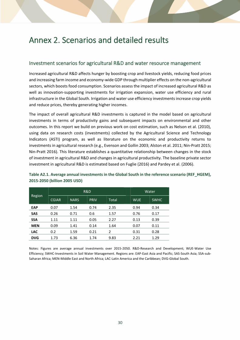
30

Annex 2. Scenarios and detailed results

Investment scenarios for agricultural R&D and water resource management

Increased agricultural R&D affects hunger by boosting crop and livestock yields, reducing food prices

and increasing farm income and economy-wide GDP through multiplier effects on the non-agricultural

sectors, which boosts food consumption. Scenarios assess the impact of increased agricultural R&D as

well as innovation-supporting investments for irrigation expansion, water use efficiency and rural

infrastructure in the Global South. Irrigation and water use efficiency investments increase crop yields

and reduce prices, thereby generating higher incomes.

The impact of overall agricultural R&D investments is captured in the model based on agricultural

investments in terms of productivity gains and subsequent impacts on environmental and other

outcomes. In this report we build on previous work on cost estimation, such as Nelson et al. (2010),

using data on research costs (investments) collected by the Agricultural Science and Technology

Indicators (ASTI) program, as well as literature on the economic and productivity returns to

investments in agricultural research (e.g., Evenson and Gollin 2003; Alston et al. 2011; Nin-Pratt 2015;

Nin-Pratt 2016). This literature establishes a quantitative relationship between changes in the stock

of investment in agricultural R&D and changes in agricultural productivity. The baseline private sector

investment in agricultural R&D is estimated based on Fuglie (2016) and Pardey et al. (2006).

Table A2.1. Average annual investments in the Global South in the reference scenario (REF_HGEM),

2015-2050 (billion 2005 USD)

Region R&D

Water

CGIAR NARS PRIV Total

WUE SWHC

EAP 0.07 1.54 0.74 2.35 0.94 0.34

SAS 0.26 0.71 0.6 1.57 0.76 0.17

SSA 1.11 1.11 0.05 2.27 0.13 0.39

MEN 0.09 1.41 0.14 1.64 0.07 0.11

LAC 0.2 1.59 0.21 2 0.31 0.28

DVG 1.73 6.36 1.74 9.83 2.21 1.29

Notes: Figures are average annual investments over 2015-2050. R&D-Research and Development; WUE-Water Use

Efficiency; SWHC-Investments in Soil Water Management. Regions are: EAP-East Asia and Pacific; SAS-South Asia; SSA-sub-

Saharan Africa; MEN-Middle East and North Africa; LAC-Latin America and the Caribbean; DVG-Global South.

31

Table A2.2. Average annual additional investments in the Global South (relative to the reference

scenario), 2015-2050 (billion 2005 USD)

Region R&D

Water

HIGH +NARS +REFF +PRIV Combined

WUE SWHC

EAP 0.02 0.11 0.06 0.22 0.41 1.75 0.15

SAS 0.15 0.11 0.13 0.18 0.57 0.96 0.21

SSA 1.74 0.33 0.10 0.02 2.19 0.16 0.27

MEN 0.04 0.30 0.06 0.04 0.44 0.22 0.21

LAC 0.12 0.14 0.07 0.06 0.39 0.58 0.20

DVG 2.08 0.99 0.42 0.52 4.01 3.66 1.03

Notes: Figures are average annual investments over 2015-2050. HIGH, HIGH+NARS, and HIGH+NARS+RE assume the same

level of increased investment from CGIAR. Regions are: EAP-East Asia and Pacific; SAS-South Asia; SSA-sub-Saharan Africa;

MEN-Middle East and North Africa; LAC-Latin America and the Caribbean; DVG-Global South.

Investments in research take time to bear fruit, as new ideas can take years to develop and spread. To

capture these lags, the investment-yield estimation model is based on the perpetual inventory

method, where research investments contribute to the stock of knowledge over time. Knowledge

decays as older technologies become obsolete or irrelevant. Productivity grows if the stock of

knowledge grows at a faster rate than the stock of knowledge decays. The lag structure in the

perpetual inventory method used here follows a gamma distribution in which R&D investments reach

peak impact ten years after initial investment and then decline over time to zero impact ten years

after peak impact. With regionally differentiated research elasticities and decay rates, these imputed

lag structures would vary by region according to existing R&D capacity and the potential trajectories

for each region. This approach allows us not only to estimate the baseline costs in research implied

under business as usual to 2050, but also to estimate additional investments needed to adapt to

climate change and make progress toward selected SDGs.

Accounting for both public and private investments, the first component of the investment gap is

computed as the difference in investments between the reference scenario and the level of

investments required to end hunger (SDG2 calorie-based target) in 2030. Investments in the scenario

analysis focus on agricultural R&D and water and soil management. In addition to food security

impacts, the impact on CO2 and non-CO2 emissions and emissions due to long-term productivity

growth in agriculture are projected based on the outcomes of the investment scenarios. In the IMPACT

modeling system, investments in agricultural R&D for productivity growth also influence projected

GHG emissions by reducing commodity prices, crop area harvested, animal numbers and fertilizer use

due to improved nitrogen use efficiency (using less nitrogen per unit of output), and by changing

cropping and livestock production patterns.

Improvements in agricultural productivity in the reference scenario are represented by exogenous

growth rates for each commodity and country, based on historical trends as well as expert opinion

about future changes. We have developed an R&D investment-yield model to assess the investment

required to achieve projected growth in agricultural productivity.

32

Yield gains were first expressed as potential changes in absolute yield levels and then translated into

differential yield growth rates used in the IMPACT modeling framework. The final endogenous yields

and output growth generated by the investment scenarios are functions of interactions between these

growth rates and projected changes in prices, demand and other factors. Projected percentage

increases in crop and livestock yields in 2030 relative to the reference scenario (REF_HGEM) are shown

in Figures A2.1 and A2.2. Agricultural productivity in sub-Saharan Africa has lagged significantly behind

the rest of the world, but with the heavy concentration of investment in agricultural R&D in this region

in the investment scenarios, both crop and livestock yield growth in sub-Saharan Africa are projected

to grow faster than other regions. Livestock yields in South Asia will also grow more rapidly than the

developing country average, from their currently relatively low levels.

Figure A2.1. Projected changes in crop yields under alternative investment scenarios, percent

difference from REF_HGEM in 2030, all crops.

Notes: WLD-World; DVG-Global South; EAP-East Asia and Pacific; SAS-South Asia; SSA-sub-Saharan Africa; MEN-Middle East

and North Africa; LAC-Latin America and the Caribbean.

33

Figure A2.2. Projected changes in livestock yields under alternative investment scenarios, percent

difference from REF_HGEM in 2030, all livestock.

Notes: WLD-World; DVG-Global South; EAP-East Asia and Pacific; SAS-South Asia; SSA-sub-Saharan Africa; MEN-Middle East

and North Africa; LAC-Latin America and the Caribbean.

Hunger and economic outcomes

The share of people at risk of hunger is the percentage of the total population in a country that is at

risk of suffering from undernourishment. This calculation is based on the empirical correlation

between the share of undernourished within the total population and the relative availability of food

and is adapted from the work done by Fischer et al. (2005) in the International Institute for Applied

Systems Analysis (IIASA) World Food System used by IIASA and FAO. This approach is equivalent to

FAO prevalence of undernourishment metric (FAO 2008). The number of hungry people is then

computed as the share of people at risk of hunger times the population. The results for the impact of

the investment scenarios are shown in Table A2.3 and are summarized in the main text above.

Sensitivity analysis run for another recent publication using IMPACT shows that the impact of

investments in agricultural R&D on hunger have a robust effect across the range of potential climate

and socioeconomic futures. Sulser et al. (2021) ran scenarios with combinations of socioeconomic

assumptions for the Shared Socioeconomic Pathways SSP1, SSP2 and SSP3, and climate assumptions

with Representative Concentration Pathways RCP4.5 and RCP8.5, using the Global Circulation Models

HADGEM2-ES (Jones et al. 2011), IPSL-CM5A-LR (Dufresne et al. 2013), MIROC-ESM (Watanabe et al.

2011), NorESM1-M (Bentsen et al. 2013; Iversen et al. 2013) and GFDL-ESM2M (Dunne et al. 2012) for

agricultural R&D investment scenarios similar to the HIGH, HIGH+NARS, AND HIGH+NARS+REFF

scenarios in this paper. The results for these investment scenarios show a reduction in the population

at risk of hunger in the developing world of 15% to 30% in 2030 and 2050, respectively, relative to the

reference scenario. The more pessimistic combinations of socioeconomic and climate assumptions

34

(SSP3, RCP8.5 and HGEM) yield larger reductions in hunger as there is more room for improvement

compared to the more optimistic scenario combinations. The results from this study are consistent

with these results, with reductions in the population at risk of hunger in the developing world in 2030

of 15% to 28%, relative to the reference scenario, and of 20% to 31% in 2050 for the HIGH, HIGH+NARS

and HIGH+NARS+REFF investment scenarios (Table A2.3).

Table A2.3. Prevalence of hunger in millions of people and as a share of the total population

(percent)

WLD DVG EAP SAS SSA MEN LAC

Population at Risk of Hunger

2010 REF_HGEM 838.1 823.3 271.3 268.5 209.5 29.3 39.5

2030 REF_HGEM 601.8 586.2 120.2 166.2 226.8 35.8 35.8

HIGH 515.1 500.3 111.7 130.7 189.8 33.3 33.2

HIGH+NARS 496.1 481.6 109.9 122.5 182.2 32.8 32.6

HIGH+NARS+REFF 433.3 419.4 103.9 96.0 156.0 31.1 30.7

HIGH+NARS+REFF+PRIV 422.3 408.5 102.2 90.3 153.4 30.7 30.1

WUE 584.6 569.2 118.1 157.0 222.4 35.2 35.1

SWHC 589.0 573.4 118.8 161.8 220.6 35.5 35.4

2050 REF_HGEM 491.6 475.9 108.8 99.8 199.5 38.2 28.8

HIGH 393.9 380.7 94.0 85.4 141.8 33.4 24.8

HIGH+NARS 376.6 364.0 91.9 83.4 130.9 32.6 24.0

HIGH+NARS+REFF 341.4 329.1 87.6 80.1 106.0 31.3 22.6


WUE 482.5 467.1 107.4 97.4 195.5 37.7 28.3

SWHC 473.4 458.0 106.8 97.4 187.3 37.5 28.0

Share at Risk of Hunger

2010 REF_HGEM 12.2 14.2 12.4 16.5 24.3 6.4 6.8

2030 REF_HGEM 7.3 8.3 5.1 8.0 17.1 5.9 5.2

HIGH 6.2 7.1 4.8 6.3 14.3 5.5 4.8

HIGH+NARS 6.0 6.8 4.7 5.9 13.7 5.4 4.7

HIGH+NARS+REFF 5.2 5.9 4.4 4.6 11.8 5.1 4.4


WUE 7.1 8.1 5.0 7.6 16.8 5.8 5.1

SWHC 7.1 8.1 5.1 7.8 16.6 5.8 5.1

2050 REF_HGEM 5.4 6.0 4.8 4.2 11.1 5.3 3.9

HIGH 4.3 4.8 4.2 3.6 7.9 4.7 3.3

HIGH+NARS 4.1 4.6 4.1 3.5 7.3 4.6 3.2

HIGH+NARS+REFF 3.7 4.2 3.9 3.4 5.9 4.4 3.0


WUE 5.3 5.9 4.8 4.1 10.9 5.3 3.8

SWHC 5.2 5.8 4.7 4.1 10.4 5.2 3.8

Notes: WLD-World; DVG-Global South; EAP-East Asia and Pacific; SAS-South Asia; SSA-sub-Saharan Africa; MEN-Middle East and North Africa; LAC-Latin America and the Caribbean.

35

Table A2.4. Average per capita incomes in the reference scenario (thousand 2005 USD per person)

and percent differences under alternative investment scenarios in 2030 and 2050


2010 REF_HGEM 9.82 5.44 8.81 2.74 1.97 9.96 9.98

2030 REF_HGEM 17.23 12.42 22.33 6.86 3.73 17.04 16.88

HIGH 0.50% 0.80% 0.50% 1.13% 3.59% 0.59% 0.20%

HIGH+NARS 0.62% 1.00% 0.62% 1.41% 4.52% 0.75% 0.25%

HIGH+NARS+REFF 1.09% 1.75% 1.10% 2.49% 7.77% 1.30% 0.45%

HIGH+NARS+REFF+PRIV 1.21% 1.93% 1.28% 2.65% 8.04% 1.45% 0.53%

WUE 0.12% 0.19% 0.15% 0.47% 0.11% 0.15% 0.02%

SWHC 0.09% 0.14% 0.13% 0.09% 0.73% 0.05% 0.04%

2050 REF_HGEM 24.82 19.62 35.29 13.22 7.22 25.82 25.65

HIGH 1.82% 2.63% 1.32% 3.05% 11.93% 1.67% 0.66%

HIGH+NARS 2.27% 3.28% 1.64% 3.82% 14.94% 2.09% 0.83%

HIGH+NARS+REFF 3.30% 4.76% 2.37% 5.62% 21.53% 3.03% 1.21%

HIGH+NARS+REFF+PRIV 4.09% 5.91% 2.98% 7.71% 23.45% 4.07% 1.65%

WUE 0.17% 0.25% 0.12% 0.64% 0.31% 0.20% 0.04%

SWHC 0.32% 0.46% 0.33% 0.22% 2.44% 0.16% 0.13%

Notes: Projected value for REF_HGEM – all other scenarios show percent change from REF_HGEM. WLD-World; DVG-Global South; EAP-East Asia and Pacific; SAS-South Asia; SSA-sub-Saharan Africa; MEN-Middle East and North Africa; LAC-Latin America and the Caribbean.

Table A2.5. Regional increase in GDP under investment scenarios in 2030 and 2050 compared to

REF_HGEM (trillion 2005 USD).


2030 HIGH 0.709 0.700 0.262 0.161 0.177 0.061 0.024

HIGH+NARS 0.885 0.873 0.325 0.200 0.223 0.077 0.030

HIGH+NARS+REFF 1.558 1.534 0.576 0.353 0.384 0.134 0.053


WUE 0.172 0.170 0.078 0.066 0.006 0.016 0.002

SWHC 0.128 0.127 0.067 0.013 0.036 0.005 0.005

2050 HIGH 4.149 4.067 1.056 0.957 1.545 0.308 0.126

HIGH+NARS 5.181 5.077 1.305 1.199 1.935 0.387 0.157

HIGH+NARS+REFF 7.524 7.365 1.890 1.763 2.789 0.560 0.229


WUE 0.395 0.387 0.095 0.200 0.040 0.037 0.008

SWHC 0.723 0.711 0.266 0.068 0.316 0.030 0.025

Notes: WLD-World; DVG-Global South; EAP-East Asia and Pacific; SAS-South Asia; SSA-sub-Saharan Africa; MEN-Middle East and North Africa; LAC-Latin America and the Caribbean.

36

Table A2.6. Aggregated commodity prices, % difference relative to REF_HGEM in 2050.

All Cereals

Fruits and Vegetables Meat Oilseeds Pulses

Roots and Tubers

2030 HIGH -7% -11% -3% -10% -6% -13% -14%

HIGH+NARS -9% -14% -4% -12% -8% -16% -17%

HIGH+NARS+REFF -15% -21% -7% -15% -12% -27% -28%

HIGH+NARS+REFF+PRIV -16% -23% -9% -16% -13% -27% -28%

WUE -1% -3% -1% 0% -1% -1% 0%

SWHC -1% -1% -1% 0% -1% -2% -2%

2050 HIGH -14% -22% -6% -20% -13% -25% -25%

HIGH+NARS -17% -25% -8% -24% -15% -30% -31%

HIGH+NARS+REFF -23% -32% -10% -27% -20% -41% -42%

HIGH+NARS+REFF+PRIV -29% -39% -20% -30% -21% -42% -43%

WUE -1% -2% 0% 0% -1% -1% 0%

SWHC -2% -3% -2% 0% -2% -3% -3%

GHG emission reductions through productivity growth

Total global GHG emissions from all sources were 52,000 MtCO2eq in 2015 (Crippa et al. 2021). Direct

GHG emissions from agricultural production, together with related emissions from land use change

and forestry, account for nearly one quarter of global GHG emissions (IPCC 2014). According to FAO

(2021a), direct agricultural emissions were about 5,450 MtCO2eq in 2015. IPCC (2013) estimates the

total direct agricultural emissions to range from 4,300 to 5,300 MtCO2eq per year, with 95%

confidence intervals spanning 3,900 to 7,000 MtCO2eq per year. According to the Food Security

Chapter of the IPCC Climate Change Land Special Report (Mbow et al. 2019), about 21-37% of total

GHG emissions are attributable to the food system, including emissions from agriculture and land use,

storage, transport, packaging, processing, retail and consumption. (Crippa et al. (2021) provide a

higher estimate of 34%, with a range of 25% to 42%). Crop and livestock activities within the farm gate

account for 9-14% of total global GHG emissions, consistent with the FAOSTAT and IPCC estimates of

direct agricultural emissions above (Mbow et al. 2019). Agriculture is also responsible for 5-14% of

total GHG emissions through its impact on land use and land use change, and 5-10% from supply chain

activities (Mbow et al. 2019). As described below, the focus of this report is on direct agricultural

emissions and the impact of investments on land use change. Changes in GHG emissions from supply

chain activities are not analyzed in this report. Although agricultural lands also generate large CO2

fluxes both to and from the atmosphere via photosynthesis and respiration, this flux is nearly balanced

on existing agriculture lands. Substantial carbon releases, however, result from the conversion of

forested land, which is accounted for under the land use change category. According to Mbow et al.

(2019), agricultural production is responsible for 5-14% of total GHG emissions through its impact on

land use and land use change, including deforestation and peatland degradation.

The GHG emissions post-processor, combined with IMPACT results, give the GHG impacts generated

by changes in crop and livestock production systems caused by agricultural productivity growth in the

37

different scenarios. The empirical approach to estimate GHG emissions uses IPCC Tier 1 and 2 factors

for GHG emissions. GHG emissions are estimated from three subcategories: synthetic fertilizers

(nitrous oxide, N2O), rice cultivation (methane, CH4), and enteric fermentation (CH4) in livestock. To

simulate emissions, we employed the IPCC Tier 1 default factors for direct N2O emissions arising from

mineral N fertilizer application to managed soils. CO2 equivalent (CO2eq) for these emissions is

computed by multiplying the amount of the GHG by its global warming potential.

Although a few efforts have been made to estimate N2O emissions by using process-based simulation

models, most have been limited to major cereal crops, such as maize, rice and wheat. To simulate

emissions from all fertilizer use, we employed the IPCC Tier 1 default factors for direct N2O emissions

arising from mineral N fertilizer application to managed soils (0.01 kg N2O-N per kg N fertilizer applied)

and to irrigated rice (0.003 kg N2O-N per kg N fertilizer applied). These factors were multiplied by the

N fertilizer consumption projected in IMPACT for each country and each crop/commodity. Note that

the N2O emissions we estimated exclude the indirect N2O emissions from nitrogen leaching and runoff

and from atmospheric nitrogen deposition.

To estimate CH4 emissions from rice production, we combined crop/commodity yields projected by

IMPACT with emission factors from Yan et al. (2009); hence, IPCC Tier 1 and Tier 2 methodologies are

employed to estimate the global CH4 emissions from rice fields. Emissions factors for this approach

include the baseline emission factor for continuously flooded fields without organic amendments, a

scaling factor for differences in the water regime during the cultivation period (e.g., single drainage

and multiple drainage), and a scaling factor for both the type of organic amendment applied (e.g., rice

straw and farmyard manure) and the amount. These CH4 emissions from rice production were first

calculated for a unit of area and then multiplied by rice production areas projected by IMPACT.

Livestock production is responsible for CH4 emissions from enteric fermentation and both CH4 and N2O

emissions from livestock manure management systems. Among several species of livestock, ruminants

such as cows, buffaloes, camels and goats are important sources of CH4 in many countries because

their ruminant digestive systems have high CH4 emission rates (IPCC 2006). Thus, CH4 emissions from

ruminants were estimated based on animal numbers projected in IMPACT (both slaughtered cattle

and dairy animals) and emission numbers from the enteric fermentation section of FAOSTAT. To

estimate emissions from the entire herd of ruminants, the projected numbers of each type of animal

(slaughter cattle, dairy cows, goats, sheep, camels and buffaloes) were multiplied by the emission

value obtained from FAOSTAT for per-head emissions from enteric fermentation.

Finally, the GHG emissions from changes in land cover driven by changes in crop area harvested and

pastureland were computed. The relationship between changes in crop area and livestock production

on the one hand and total cropland, pasture and forest area on the other hand were derived from

simulations that linked IMPACT and LandSHIFT. LandSHIFT is a land use land cover change model

(Schaldach et al. 2011). The estimated changes in land use driven by changes in area and livestock

production were then combined with the Tier 1 GHG emissions coefficients for the relevant land use

types to compute the estimated GHG emissions changes.

38

Table A2.7. Projected GHG emissions reductions and sequestration per year from agriculture due to

investments in productivity growth, HIGH+NARS+REFF+PRIV, relative to the reference scenario.

Emissions Sources MtCO₂eq per year

2030 2050

Fertilizer (N2O) 110 131

Rice (CH4) 27 53

Livestock: (CH4) 154 313

Total non-CO2 GHG emissions reduction 291 497

Reductions in C emissions due to less land use change 111 248

Source: IMPACT modeling analysis.

Technical options for climate change mitigation

Restoration of agricultural soils is not included. Following IPCC guidelines for accounting for GHG

emissions in agriculture (IPCC 2006), upstream and downstream emissions such as production of

fertilizer and other inputs and value chain emissions are not included. The technical options

considered are:

• Improved cropland management. This is an important potential method to reduce N2O

emissions and sequester CO2. These can be achieved through agronomy (crop rotation and

cover crops); conservation tillage and residue management; improved water management

to reduce fertilizer runoff; and improved nutrient management through precision

agriculture, advanced types of fertilizer, nitrogen use efficient new crop varieties and

stabilized N sources (polymer-coated urea and nitrification inhibitors).

• Improved rice management for reduction of methane (CH4). This includes midseason

drainage of rice paddies and alternate wetting and drying.

• Pasture management, which can reduce GHG emissions through improved grasses and

pasture management, improved manure management and use of legumes.

• Livestock management, which reduce CH4 emissions with improved feeding practices and

feed additives, improved manure management systems, and breeding and long-term

management.

The assessment of technical options for GHG mitigation is based on data and research outcomes

available from IPCC documents and other publications. Sources consulted include IPCC (2020, 2016,

2014), Beach et al. (2015), Herrero et al. (2016), Wollenberg et al. (2016), Smith et al. (2008, 2018),

Frank et al. (2018), Smith et al. (2013), Del Grosso and Cavigelli (2012), Havlík et al. (2014) and EPA

(2019). Key parameters considered in the assessment include the potential savings in tCO2eq per

hectare or per animal unit from adoption of technical options; the rate of adoption of technical options

in terms of percentage of area or herd; and the cost of investment in mitigation from each technical

option in USD per tCO2eq. Investment costs include incremental annualized capital costs where

applicable (many of the mitigation practices are more focused on changes in practices and inputs than

capital expenditures) and estimated incremental changes in the annual costs of agricultural labor,

fertilizer and other inputs. Following the practice in these sources, costs do not include revenue

changes for farmers due to productivity increases or decreases related to the application of a

39

technology (Frank et al. 2018). The assumptions regarding the range of values for the key parameters

are shown in Table A2.8.

Table A2.8. Assumptions for analysis of technical climate mitigation potential and costs: range of

values used.

(a) Cropland, rice and grassland/pasture management.

Potential

Adoption

in 2030

Potential

Adoption

in 2050

Cost in

2030

Cost in

2050

CO2

mitigation

potential

(biophysical)

CH4

mitigation

potential

(biophysical)

NO2

mitigation

potential

(biophysical)

(% of crop

area

harvested)

(% of crop

area

harvested)

(USD/tC

O2eq)

(USD/tC

O2eq)

(tCO2eq per

ha per yr)

(tCO2eq per

ha per yr)

(tCO2eq per

ha per yr)

CROPLAND

MANAGEMENT

- Agronomy 50-70 45-100 10-15 11-18 0.40-0.58 n/a 0.04-0.085

- Tillage and

residue

management

50-80 45-100 9-15 10-18 0.24-0.40 n/a 0.02-0.06

- Nutrient

management

50-80 45-100 8-15 9-18 0.20-0.30 n/a 0.07-0.12

- Water

management

50-70 45-100 10-20 12-23 0.04-0.05 n/a 0.05-0.075

RICE

MANAGEMENT

65-80 65-100 6-9 7-10 n/a 1.51-1.90 n/a

GRASSLAND/

PASTURE

MANAGEMENT

20-40 20-40 7-10 8-12 0.40-0.46 0.01-0.04 n/a

(b) Livestock management.

Cost in 2030 Cost in 2050 Livestock CH4

(% mitigation

potential)

Livestock CH4

(% mitigation

potential)

(USD/tCO2eq) (USD/tCO2eq) Global South Global North

LIVESTOCK SECTOR 8 - 12 9 - 13

- Improved feeding

practices, additives, etc.

5-10 10-12

- Manure management 2-4 4-5

- Breeding and long-term

management

2-4 3-4

Note: n/a= not applicable. Sources: Estimated ranges of parameter values are drawn from IPCC (2016, 2014), Beach et al.

(2015), Herrero et al. (2016), Wollenberg et al. (2016), Smith et al. (2008), Frank et al. (2018), Smith et al. (2013, 2018), Del

Grosso and Cavigelli (2012), Havlík et al. (2014) and EPA (2019).

40

In agriculture, there is a relationship between the amount paid for GHG emission reductions (i.e. the

price per tCO2eq) and the level of mitigation realized. The economic potential for mitigation options

in agriculture increases as the carbon price rises. For this analysis we assess the potential for GHG

mitigation from adoption of technical mitigation options at a carbon price of USD 70/tCO2eq. This

carbon price was chosen for assessment based on review of the literature as a carbon price that would

potentially generate GHG emissions reductions that would be consistent with the Paris Agreement

pathways (see, for example, Frank et al. 2018; Beach et al. 2015; Del Grosso and Cavigelli 2012; Smith

et al. 2014).

Based on these parameters we compute the potential mitigation in MtCO2eq per year in 2030 and

2050, and the annual cost of investment in mitigation in 2030 and 2050, in million USD per year. The

key parameters vary across sources and ranges are reported in many of the sources. To capture this

variability, calculations were made for a series of combinations of the parameters to assess a

distribution of potential outcomes. These results allow us to compute the investment required to

generate GHG emissions reductions consistent with the Paris Agreement pathways. The investment

requirements represent the total carbon payments or payments for environmental services that need

to be paid to induce the adoption of the technical options needed to generate mitigation consistent

with a 2°C climate trajectory.

GHG emission reductions and sequestration through the adoption of technical

options

Figures A2.3-A2.5 show the distribution of estimated potential mitigation of GHG emissions from

technical options at a carbon price of USD 70/tCO2eq. Figure A2.6 shows the investment required to

generate this level of mitigation. In these box-and-whisker diagrams, the box shows the upper and

lower quartiles of the distribution of the results, and the whiskers (the lines extending from the boxes)

indicate variability outside the upper and lower quartiles (defined here as highest and lowest values

within 1.5 times the interquartile range). Any dots outside the whiskers represent outliers. The means

of the distribution are shown as dots within the boxes and the medians are shown as horizontal lines

in the boxes.

As can be seen in Figure A2.3, the mean non-CO2 technical mitigation economic potential in 2030 is

715 MtCO2eq per year, with a range of 606 MtCO2eq per year to 815 MtCO2eq per year; the mean

potential in 2050 is 783 MtCO2eq per year, with a range of 647 MtCO2eq per year to 901 MtCO2eq per

year. Comparisons with the literature are not precise because of the different methods employed for

these estimations, but comparisons are nevertheless useful. Del Grosso and Cavigelli (2012) estimated

that the potential for non-CO2 agricultural mitigation from technical options at a carbon price of USD

50/tCO2eq is 693 MtCO2eq per year in 2030; EPA (2019) estimates savings of 593 MtCO2eq per year in

2030 at “increasing prices”; Frank et al. (2018) estimate that adoption of technical options in 2030 can

deliver direct non-CO2 emission savings of 500 MtCO2eq per year at USD 40/tCO2eq, and 800 MtCO2eq

per year at USD 100/tCO2eq in 2030; and about 850 MtCO2eq per year at USD 100/tCO2eq in 2050.

Thus, the estimates of economic potential made here are within the range found in the literature. The

total cost (investment required in carbon payments) to generate this level of mitigation is shown in

Figure A2.6. The mean cost of technical mitigation is USD 6.5 billion per year in 2030, with a range of

USD 5.4-7.9 billion per year. We also ran a sensitivity analysis of the non-CO2 technical mitigation

economic potential with respect to carbon prices of USD 50/tCO2eq and USD 100/tCO2eq. Although

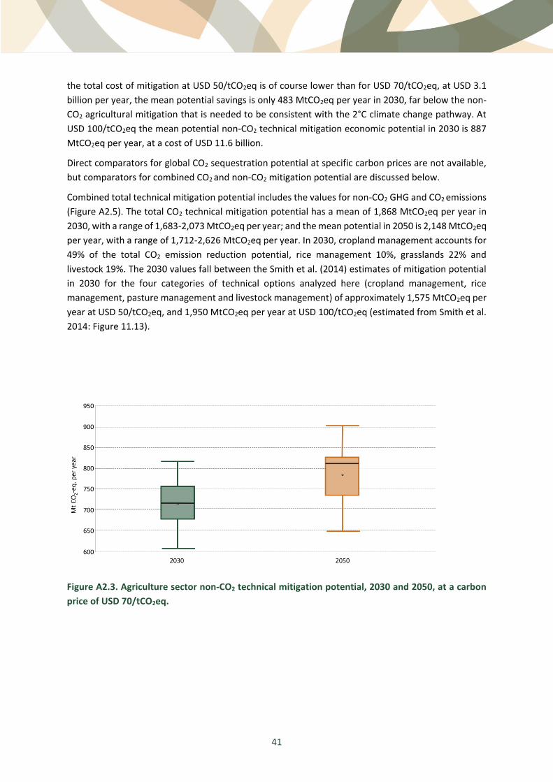
41

the total cost of mitigation at USD 50/tCO2eq is of course lower than for USD 70/tCO2eq, at USD 3.1

billion per year, the mean potential savings is only 483 MtCO2eq per year in 2030, far below the non-

CO2 agricultural mitigation that is needed to be consistent with the 2°C climate change pathway. At

USD 100/tCO2eq the mean potential non-CO2 technical mitigation economic potential in 2030 is 887

MtCO2eq per year, at a cost of USD 11.6 billion.

Direct comparators for global CO2 sequestration potential at specific carbon prices are not available,

but comparators for combined CO2 and non-CO2 mitigation potential are discussed below.

Combined total technical mitigation potential includes the values for non-CO2 GHG and CO2 emissions

(Figure A2.5). The total CO2 technical mitigation potential has a mean of 1,868 MtCO2eq per year in

2030, with a range of 1,683-2,073 MtCO2eq per year; and the mean potential in 2050 is 2,148 MtCO2eq

per year, with a range of 1,712-2,626 MtCO2eq per year. In 2030, cropland management accounts for

49% of the total CO2 emission reduction potential, rice management 10%, grasslands 22% and

livestock 19%. The 2030 values fall between the Smith et al. (2014) estimates of mitigation potential

in 2030 for the four categories of technical options analyzed here (cropland management, rice

management, pasture management and livestock management) of approximately 1,575 MtCO2eq per

year at USD 50/tCO2eq, and 1,950 MtCO2eq per year at USD 100/tCO2eq (estimated from Smith et al.

2014: Figure 11.13).

Figure A2.3. Agriculture sector non-CO2 technical mitigation potential, 2030 and 2050, at a carbon

price of USD 70/tCO2eq.

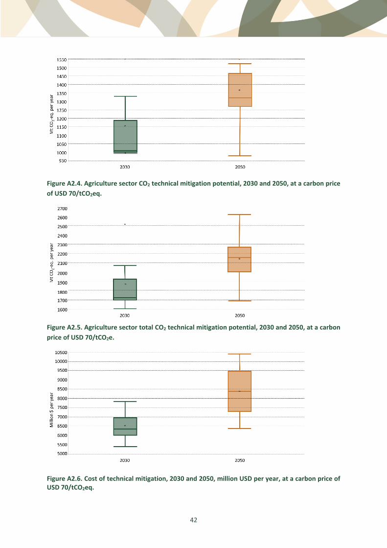
42

Figure A2.4. Agriculture sector CO2 technical mitigation potential, 2030 and 2050, at a carbon price

of USD 70/tCO2eq.

Figure A2.5. Agriculture sector total CO2 technical mitigation potential, 2030 and 2050, at a carbon

price of USD 70/tCO2e.

Figure A2.6. Cost of technical mitigation, 2030 and 2050, million USD per year, at a carbon price of USD 70/tCO2eq.

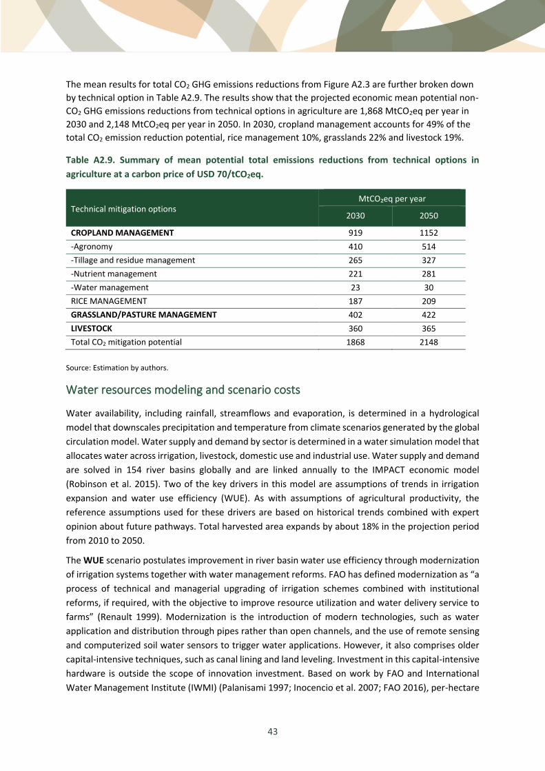
43

The mean results for total CO2 GHG emissions reductions from Figure A2.3 are further broken down

by technical option in Table A2.9. The results show that the projected economic mean potential non-

CO2 GHG emissions reductions from technical options in agriculture are 1,868 MtCO2eq per year in

2030 and 2,148 MtCO2eq per year in 2050. In 2030, cropland management accounts for 49% of the

total CO2 emission reduction potential, rice management 10%, grasslands 22% and livestock 19%.

Table A2.9. Summary of mean potential total emissions reductions from technical options in

agriculture at a carbon price of USD 70/tCO2eq.

Technical mitigation options MtCO₂eq per year

2030 2050

CROPLAND MANAGEMENT 919 1152

-Agronomy 410 514

-Tillage and residue management 265 327

-Nutrient management 221 281

-Water management 23 30

RICE MANAGEMENT 187 209

GRASSLAND/PASTURE MANAGEMENT 402 422

LIVESTOCK 360 365

Total CO2 mitigation potential 1868 2148

Source: Estimation by authors.

Water resources modeling and scenario costs

Water availability, including rainfall, streamflows and evaporation, is determined in a hydrological

model that downscales precipitation and temperature from climate scenarios generated by the global

circulation model. Water supply and demand by sector is determined in a water simulation model that

allocates water across irrigation, livestock, domestic use and industrial use. Water supply and demand

are solved in 154 river basins globally and are linked annually to the IMPACT economic model

(Robinson et al. 2015). Two of the key drivers in this model are assumptions of trends in irrigation

expansion and water use efficiency (WUE). As with assumptions of agricultural productivity, the

reference assumptions used for these drivers are based on historical trends combined with expert

opinion about future pathways. Total harvested area expands by about 18% in the projection period

from 2010 to 2050.

The WUE scenario postulates improvement in river basin water use efficiency through modernization

of irrigation systems together with water management reforms. FAO has defined modernization as “a

process of technical and managerial upgrading of irrigation schemes combined with institutional

reforms, if required, with the objective to improve resource utilization and water delivery service to

farms” (Renault 1999). Modernization is the introduction of modern technologies, such as water

application and distribution through pipes rather than open channels, and the use of remote sensing

and computerized soil water sensors to trigger water applications. However, it also comprises older

capital-intensive techniques, such as canal lining and land leveling. Investment in this capital-intensive

hardware is outside the scope of innovation investment. Based on work by FAO and International

Water Management Institute (IWMI) (Palanisami 1997; Inocencio et al. 2007; FAO 2016), per-hectare

44

investment cost for modernization of irrigation systems is USD 2,144 for East, South, Southeast and

Central Asia; USD 4,311 for sub-Saharan Africa and Latin America; and USD 953 for the Middle East

and North Africa. These estimates are likely too high for the more recent, less capital-intensive

modernization investments, but there is not adequate recent data to update the estimates. It is

assumed that modernization is phased in over time, reaching 80% of irrigation systems by 2050.

For the SWHC scenario, many technologies and management strategies for soil water conservation

are available. Soil and water conservation options for increasing plant water uptake capacity include

bunds, ridges, broad-beds and furrows, micro basins, runoff strips, terracing and contour cultivation.

Water harvesting options include surface micro dams, subsurface tanks, farm ponds, percolation dams

and tanks, diversion, and recharging structures. Evaporation management includes dry planting,

mulching, conservation agriculture and vegetative bunds (Cervigni and Morris 2016). These

technologies have a wide range of costs and data is relatively sparse. Costs estimates range from USD

44/ha to USD 212/ha, depending on the type and location of interventions (Cervigni and Morris 2016;

IWMI 2012; McCarthy 2011). For this analysis, we assume that a range of these interventions is phased

in to 70% of rainfed area by 2050, with an average mean of USD 109/ha. The required innovation

investments are the smart subsidies or payment for environmental services required to incentivize

adoption, estimated at 30% of the total cost, drawing upon Cervigni and Morris (2016).

IMPACT uses the concept of basin efficiency, which is defined as the ratio of beneficial water depletion

(crop evapotranspiration and salt leaching) to total irrigation water depletion at the basin scale, taking

account of return flows from irrigation within the river basin. In the WUE scenario, basin efficiency in

future years is projected to increase at a prescribed rate depending on investment in water

management. For the WUE scenario, basin efficiencies improvements are phased in to increase by 15

percentage points. The SWHC scenario simulates the benefits of technologies, such as water

harvesting, that increase the water holding capacity of soil or otherwise make precipitation more

readily available to plants (i.e., effective precipitation). Improvements vary by region due to the

different levels at which these kinds of technologies are currently being applied, with a maximum

increase in effective precipitation of 5-15% by 2045.

Table A2.10. Global water use under alternative scenarios, billion cubic meters, projected to 2030

and 2050.

BCM

% diff from REF_HGEM

2010 2030 2050

2030 2050

Bluewater REF_HGEM 1,731 1,890 2,063 0.00 0.00

HIGH 1,731 1,887 2,056 -0.11 -0.32

HIGH+NARS 1,731 1,887 2,054 -0.14 -0.40

HIGH+NARS+REFF 1,731 1,885 2,051 -0.24 -0.54

HIGH+NARS+REFF+PRIV 1,731 1,884 2,044 -0.30 -0.91

WUE 1,731 1,722 1,871 -8.86 -9.30

SWHC 1,731 1,865 2,010 -1.30 -2.56

Greenwater REF_HGEM 4,440 4,982 5,440 0.00 0.00

HIGH 4,440 4,961 5,384 -0.43 -1.04

HIGH+NARS 4,440 4,956 5,373 -0.53 -1.23

HIGH+NARS+REFF 4,440 4,940 5,355 -0.85 -1.56

45

BCM

% diff from REF_HGEM

2010 2030 2050

2030 2050

Greenwater HIGH+NARS+REFF+PRIV 4,440 4,932 5,317 -0.99 -2.26

WUE 4,440 4,971 5,427 -0.23 -0.23

SWHC 4,440 5,103 5,692 2.43 4.64

Total REF_HGEM 6,171 6,872 7,503 0.00 0.00

HIGH 6,171 6,848 7,440 -0.34 -0.84

HIGH+NARS 6,171 6,843 7,427 -0.42 -1.01

HIGH+NARS+REFF 6,171 6,825 7,407 -0.68 -1.28

HIGH+NARS+REFF+PRIV 6,171 6,816 7,361 -0.80 -1.89

WUE 6,171 6,693 7,298 -2.60 -2.73

SWHC 6,171 6,968 7,702 1.40 2.66

Table A2.11. Regional water use under alternative scenarios, billion cubic meters, projected to 2030

and 2050.

Scenario BCM % diff from REF_HGEM

2010 2030 2050

2030 2050

EAP Bluewater WUE 416 379 383 -10.46 -12.09

SWHC 416 411 412 -2.93 -5.52

Greenwater WUE 1252 1358 1443 -0.18 -0.18

SWHC 1252 1388 1499 2.01 3.70

Total WUE 1668 1737 1826 -2.62 -2.94

SWHC 1668 1799 1911 0.84 1.56

SAS Bluewater WUE 659 663 711 -6.64 -6.30

SWHC 659 704 747 -0.89 -1.47

Greenwater WUE 847 927 985 -0.39 -0.30

SWHC 847 954 1030 2.52 4.18

Total WUE 1506 1590 1696 -3.10 -2.91

SWHC 1506 1658 1777 1.04 1.73

SSA Bluewater WUE 71 88 125 -11.93 -14.14

SWHC 71 97 139 -2.32 -4.93

Greenwater WUE 697 859 1024 -0.13 -0.15

SWHC 697 909 1138 5.67 11.05

Total WUE 768 947 1149 -1.36 -1.89

SWHC 768 1007 1277 4.84 9.06

MENA Bluewater WUE 221 213 230 -12.14 -11.01

SWHC 221 242 258 -0.14 -0.25

Greenwater WUE 86 90 91 -0.27 -0.38

SWHC 86 93 97 3.19 6.18

Total WUE 306 303 321 -8.91 -8.23

SWHC 306 335 355 0.76 1.43

LAC Bluewater WUE 137 132 152 -20.08 -21.23

SWHC 137 162 184 -1.88 -4.51

Greenwater WUE 764 940 1111 -0.24 -0.28

SWHC 764 960 1153 1.90 3.56

Total WUE 901 1072 1262 -3.19 -3.37

SWHC 901 1122 1337 1.34 2.37

46

Agricultural water pollution

Agricultural activities contribute large amounts of nitrogen (N) and phosphorus (P), which make their

way into water bodies. High risks from water pollution mean that adverse impacts on humans, the

environment and the economy are likely to occur. We assess the impact of agriculture on these

pollutants using IFPRI's global water quality model (IGWQM) linked to IMPACT agricultural projections.

Global agricultural non-point source N and P loadings are estimated for the base year on a half-degree

latitude-longitude grid, accounting for both crop production and livestock production systems.

Projected loadings for crops are a function of growth in fertilizer use and rates of change in fertilizer

use efficiency. The total quantities of livestock excreta and the quantities of excreta recycled to

cropland as manure, and resultant N and P loadings, are simulated according to projected livestock

animal population size in 2050, recycling rate, and efficiency of management of livestock waste.

Alternative investments in agricultural R&D influence the outcomes for N and P loadings through their

impact on cropped area, fertilizer use and livestock production, and these outcomes are assessed in

the scenarios. However, bigger improvements in N and P use efficiency may be possible through

increased investment in breeding for enhanced nutrient use efficiency; adoption of sustainable

agricultural methods such as nutrient efficient crop varieties and fertilizers formulated for more

efficient nutrient uptake; adoption of advanced irrigation technology and improved water

management; conservation tillage; and improved management of the nutrient cycle for recycling and

re-use in the livestock sector.

In this model, global agricultural non-point source N and P loadings were estimated for the base year

on a half-degree latitude-longitude grid, accounting for both crop production and livestock production

systems. Projected loadings for crops are a function of growth in fertilizer use and rates of change in

fertilizer use efficiency. The total quantities of livestock excreta and the quantities of excreta recycled

to cropland as manure and resultant N and P loadings are simulated according to projected livestock

animal population size in 2050, recycling rate, and efficiency of management of livestock waste (Xie

and Ringler 2017; IFPRI and Veolia 2015).

Agricultural non-point loadings in the Global South in the base year of 2005 were 55 Mt for N and 2.6

Mt for P. Of this, 44 Mt of N and 1.8 Mt of P were from crops, and 12 Mt of N and 0.8 Mt of P were

from livestock (Rosegrant et al. 2017). The Global South accounted for 79% of global N loadings and

84% of P loadings in the base year. East Asia and Pacific accounted for one third of global N loadings

and South Asia one quarter. The share of the Global South in N loadings increases to 82% in 2030,

while the share of P loadings stays nearly constant. In the REF_HGEM reference scenario, global N

loadings increase to 76.8 Mt in 2030 and 89.4 Mt in 2050, and P increases to 3.4 Mt in 2030 and 4.3

Mt in 2050. Growth in GDP, population, income, crop and livestock production and fertilizer use drives

these substantial increases in pollution.

We develop an alternative scenario, incorporating the improvements in N use and P use efficiency due

to productivity growth, using the IMPACT model and improvements from adoption of technical

options. Alternative investments in agricultural R&D for productivity growth influence the outcomes

for N and P loadings through their impact on cropped area, fertilizer use and livestock production, and

these outcomes are assessed using the HIGH+NARS+REFF+PRIV scenario. The estimated

improvements are a 12% improvement in N use efficiency in 2030, and a 15% improvement in 2050,

compared to the reference scenario; and a 7% increase in P use efficiency in 2030, and an 8% increase

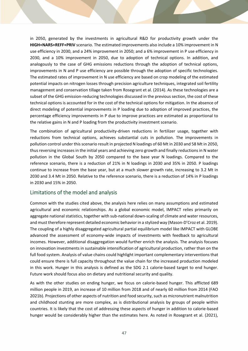
47

in 2050, generated by the investments in agricultural R&D for productivity growth under the

HIGH+NARS+REFF+PRIV scenario. The estimated improvements also include a 10% improvement in N

use efficiency in 2030, and a 24% improvement in 2050; and a 6% improvement in P use efficiency in

2030, and a 10% improvement in 2050, due to adoption of technical options. In addition, and

analogously to the case of GHG emissions reductions through the adoption of technical options,

improvements in N and P use efficiency are possible through the adoption of specific technologies.

The estimated rates of improvement in N use efficiency are based on crop modeling of the estimated

potential impacts on nitrogen losses through precision agriculture techniques, integrated soil fertility

management and conservation tillage taken from Rosegrant et al. (2014). As these technologies are a

subset of the GHG emission-reducing technologies discussed in the previous section, the cost of these

technical options is accounted for in the cost of the technical options for mitigation. In the absence of

direct modeling of potential improvements in P loading due to adoption of improved practices, the

percentage efficiency improvements in P due to improve practices are estimated as proportional to

the relative gains in N and P loading from the productivity investment scenario.

The combination of agricultural productivity-driven reductions in fertilizer usage, together with

reductions from technical options, achieves substantial cuts in pollution. The improvements in

pollution control under this scenario result in projected N loadings of 60 Mt in 2030 and 58 Mt in 2050,

thus reversing increases in the initial years and achieving zero growth and finally reductions in N water

pollution in the Global South by 2050 compared to the base year N loadings. Compared to the

reference scenario, there is a reduction of 21% in N loadings in 2030 and 35% in 2050. P loadings

continue to increase from the base year, but at a much slower growth rate, increasing to 3.2 Mt in

2030 and 3.4 Mt in 2050. Relative to the reference scenario, there is a reduction of 14% in P loadings

in 2030 and 15% in 2050.

Limitations of the model and analysis

Common with the studies cited above, the analysis here relies on many assumptions and estimated

agricultural and economic relationships. As a global economic model, IMPACT relies primarily on

aggregate national statistics, together with sub-national down-scaling of climate and water resources,

and must therefore represent detailed economic behavior in a stylized way (Mason-D’Croz et al. 2019).

The coupling of a highly disaggregated agricultural partial equilibrium model like IMPACT with GLOBE

advanced the assessment of economy-wide impacts of investments with feedback to agricultural

incomes. However, additional disaggregation would further enrich the analysis. The analysis focuses

on innovation investments in sustainable intensification of agricultural production, rather than on the

full food system. Analysis of value chains could highlight important complementary interventions that

could ensure there is full capacity throughout the value chain for the increased production modeled

in this work. Hunger in this analysis is defined as the SDG 2.1 calorie-based target to end hunger.

Future work should focus also on dietary and nutritional security and quality.

As with the other studies on ending hunger, we focus on calorie-based hunger. This afflicted 689

million people in 2019, an increase of 10 million from 2018 and of nearly 60 million from 2014 (FAO

2021b). Projections of other aspects of nutrition and food security, such as micronutrient malnutrition

and childhood stunting are more complex, as is distributional analysis by groups of people within

countries. It is likely that the cost of addressing these aspects of hunger in addition to calorie-based

hunger would be considerably higher than the estimates here. As noted in Rosegrant et al. (2021),

48

broader malnutrition problems, together with the continued transformation of food systems in

developing countries, requires wider-ranging approaches and interventions to improving nutritional

outcomes than have been used historically. Reducing the impact of these factors would require

changes beyond the agricultural sector, including planning, transportation, public health, food

production and marketing (Caballero 2007; Ruel et al. 2017). Interventions and policies should take

account of the need for more sustainable diets that would include a sufficient supply of micronutrient-

rich foods without excessive consumption of energy-dense, nutrient-poor foods (Kearney 2010). In

promoting nutrition and health-driven policies, it will be important to target those most in need,

particularly children and marginalized populations underserved by essential health services.

Furthermore, filling the knowledge gaps through research, scaling innovation solutions and promoting

partnerships across health, nutrition and agriculture will be important (Fan et al. 2019).

The potential gains from investment in agricultural R&D and water resources are susceptible to

uncertainty in governance and the fragility of states. The SSPs focus their narratives on long-running

trends in the global economy, which, while helpful for exploring scenarios around climate change and

long-term drivers in the food system like agricultural R&D, do not include other drivers that are

important to global food security. For example, extreme social and environmental events, such as the

COVID-19 pandemic, will result in year-to-year variability and alter trajectories, at least in the short

run. These events can displace millions while destroying human, physical, natural and social capital

and limiting the capacity of societies to effectively function. Although the projections here do not

assume effective or improved governance, a worsening of governance and conflict can slow the

projected growth (Mason-D’Croz et al. 2019).

The focus of our GHG emissions analysis is on emissions in agriculture consistent with sustainable

agriculture intensification trajectory for closing the investment gap. It does not focus on a food

systems trajectory, including changes in cold storage and diets, or emissions from transportation,

downstream processing of food, the manufacture of tractors and fertilizer or other relevant inputs.

Emissions from these sources are included by IPCC guidelines in other, non-agricultural sectors such

as transport and energy. Land use change and deforestation emissions driven by agriculture were

accounted for to the extent that they are generated by the investments analyzed in this report.

In most analyses of technical options for mitigation that we draw upon here, some of the options have

low or even negative costs in specific regions. This occurs when the net revenues associated with an

option are positive, indicating that the practice would be profitable even in the absence of mitigation

incentives such as carbon payments or targeted subsidies (Beach et al. 2015). It is therefore necessary

to also address potential barriers that may need to be overcome to achieve adoption options that

have low or negative costs, and that also hinder adoption of higher cost options even with mitigation

incentives. These barriers may include institutional problems, lack of property rights, risk aversion

among agricultural producers, market imperfections and regulatory or legal issues (Beach et al. 2015).

Giller et al. (2009), for example, point to farm-level constraints to adoption of conservation tillage for

soil sequestration in Africa. These include decreased yields often observed, increased labor

requirements when herbicides are not used, a shift of the labor burden to women, limited access to

external inputs, and a lack of mulch due to both low productivity and the priority given to feeding of

livestock with crop residues.

49

Constraints can also arise in the implementation of carbon sequestration programs (Pannell 2021).

Soil sequestration is a one-off process, with soil carbon increasing up to a new equilibrium level after

about 20-30 years and then stopping. However, the adoption of the management regime needs to be

maintained to avoid releasing the sequestered carbon; this means that while costs continue to be

incurred, new benefits that would justify further payments do not. Additionality therefore needs to

be determined, so that management options undertaken by farmers are additional to what they would

do anyway. If they are not additional, then carbon payments will not contribute to climate change

mitigation. Monitoring and measuring soil carbon stored in soils is also costly, requiring regular soil

testing to confirm that carbon has been sequestered. Measurement is costlier when it needs to be

done for multiple small farms. Innovations in measurement through advances in information and

communications technologies (ICT), including less expensive soils and remote sensing, could help

reduce the costs. Managing carbon sequestration for groups of farmers rather than individual farmers

could also be more cost effective (Pannell 2021).

50

Annex 3. Discussion of supporting policies and

investments

Agricultural value chains

Innovations and investments in the value chain will improve the prospects for meeting the SDG2,

SDG6, SDG13 and Paris Agreement targets. Infrastructure investments, including in rural roads,

electricity cell phone towers, markets, cold chains and processing facilities have important impacts on

input and output markets. Innovations and investments in the value chain can make the outputs of

agricultural R&D investments more profitable for farmers and generate higher social returns to

agricultural R&D investments. Input and output market investments can reduce marketing margins

and post-harvest losses of food, thereby generating substantial production and income gains and

potentially significantly reducing hunger. It is likely that expanded investments in these items will

require partnerships with the private sector. Aggregating mechanisms need to be put in place, for

example, through cooperatives that can help ensure that economies of scale for inspection, packaging,

food safety regimes and quality management are achieved competitively. Such cooperatives can also

lower costs for agricultural inputs such as seeds and chemicals and can also support microfinance

services.

Farmers need timely and reliable information about markets. In addition to information on prices, a

whole range of business-related information is essential, such as who the buyers are and what their

terms and conditions for doing business are. Market information services have often suffered from

problems related to the timeliness and accuracy of the information provided. Digital information

systems linked to farmer mobile phones can increase access to timely information, improve links

between farmers and processors, and reduce transport costs, thereby reducing post-harvest losses.

(USAID 2017). In addition to market information services, advanced digital technologies – such as

satellite imaging, remote sensing and in-field sensors – can support precision farming based on

observation of, and response to, intra-field variations that guide the efficient application of inputs and

improve productivity and farm income. However, there are many constraints to raising funds for

advanced technologies to benefit small farmers and improve input and output markets in the value

chain, and solving these constraints may require innovations in financial instruments and approaches.

Finance

Among other constraints, low agricultural productivity in the Global South is related to smallholder

farmers’ lack of capital and access to affordable credit. The unmet demand for smallholder finance is

considerable: the credit gap for smallholder farmers in the Global South is estimated at about USD

170 billion per year (Initiative for Smallholder Finance 2019). In the past two decades there has been

a decline in the provision of agricultural finance for smallholders by governments in many parts of the

world. In some cases, this gap has been replaced by credit cooperatives, microfinance institutions,

finance through the value chain by contract farming arrangements, and, occasionally, by commercial

banks. Nevertheless, access to financial services by smallholders remains limited (Committee on

51

Agriculture 2010). IFPRI (2021, forthcoming), compares access to financial services between country

groups in relation to the performance in poverty and malnutrition alleviation, and find that access to

financial institutions is associated with effective poverty alleviation. The links between access to

financial institutions and reduction of undernourishment are weaker, although access to credit or

borrowing money from a financial institution is related to better performance in poverty alleviation.

The importance of access to financial services is indicative of the importance of private sector

investments in meeting the investment targets, but significant constraints have held back private

participation in the agricultural sector. Investments in agriculture compete with other sectors based

on the attractiveness of the risk-return profile. This depends on a stable revenue stream and how the

range of risks related to agricultural investments are shared between the public and private actors.

Several factors have inhibited private sector investment in agriculture, including relatively low rates

of return and perceived high financial risks due to the uncertainty in returns in the agricultural sector

(Svendsen et al. 2003). Several financial mechanisms for investment in agriculture are promising.

These include green and blue bonds, payment for ecosystem services, and blended public and private

finance. Blended finance, which strategically uses development finance or public funding to mobilize

additional finance towards sustainable development in the Global South, is a promising approach to

scale up private sector financing for water (OECD 2018).

Extension

The quality of the extension system is an important factor in supporting the adoption and

effectiveness of new technologies, potentially increasing the benefits of the investment analyzed here.

Extension services in the Global South have changed significantly over the past four decades,

increasingly moving from a traditional emphasis on technology transfer and farm management

information, supplied by the public sector, to a broader public and private advisory service model with

increasing participation of the private sector (dealing with agricultural inputs agribusiness, and

financial services), non-governmental organizations, producer groups, cooperatives and associations,

and ICT services (Blum et al. 2020, cited in IFPRI 2021, forthcoming). Further expansion of extension

services into marketing, food safety, and the establishment of closer links with agri-food industries

and related areas would be beneficial (Committee on Agriculture 2010). Social networks and farmer-

to-farmer extension have been growing in Africa, and evidence shows that they increase the

effectiveness of extension (Takahashi et al. 20209). A cross-country analysis of extension services

shows that the best performing countries in poverty alleviation have better education facilities, a

greater focus by extension services on natural resources and climate change, and prioritize women

and young adult farmers. In the case of malnutrition, the key difference between groups of

performance is that best performing countries prioritize rural women in the areas of nutrition and

health (IFPRI 2021, forthcoming).

Gender-responsive policies and investments

Achieving global food security and nutrition, promoting sustainable agriculture and addressing climate

change are inextricably linked with gender equality and women’s empowerment. If gender is not

adequately considered in agricultural R&D systems as well as extension and other information

dissemination, it will be impossible to meet the food needs of future populations or ensure that

agricultural productivity translates into improved welfare for the poor. As such, gender equity in

52

agricultural R&D systems is a matter of development effectiveness that can benefit women, men and

their families alike (Bryan and Garner 2020; Meinzen-Dick et al. 2011). Beyond access to resources and

information, it is important that women scientists also participate more actively in agricultural

research development. Although female participation in agricultural research has improved in recent

years, Beintema and Stads (2017) report that women remain less likely to hold research management

positions than their male colleagues in much of sub-Saharan Africa, for example. As a result, women

have less influence in policy- and decision-making processes, making it challenging to reflect gendered

needs at the outset of the technology generation process.

While progress in reducing gender gaps in agriculture have been made, and women comprise a

significant share of the agricultural labor force, they continue to have less access to productive

resources, including land, labor and irrigation water, to new technologies and to services like

information and financial services. Women also have less decision-making authority and fewer

opportunities given their combined domestic and productive responsibilities (Bryan and Garner 2020;

Blackmore 2021). In addition to policies and investments to increase women’s access to a range of

resources and services, cultural power imbalances and intra-household dynamics that limit women’s

decision-making agency should be addressed (Blackmore et al. 2018; FAO 2019).

Evidence shows that increasing women’s access to land, financial and natural resources and

information, in addition to a more equitable distribution of new technology, could positively impact

women’s ability to produce and gain access to food. This, in turn, can positively impact the nutritional

status of the entire household (Agarwal 2018; Lodin et al. 2014; Blackmore 2021). Bryan et al. (2021)

finds that gendered differences in awareness and adoption of climate smart agricultural practices in

southwestern Bangladesh were linked with low access to key information sources by women farmers.

Moreover, women were more likely than men to adopt some climate smart practices, particularly

those related to their gendered roles, such as improved livestock feeding practices and grain storage,

when they became aware of adaptation options. The results suggest that greater efforts to reach both

men and women with information on climate smart agriculture would increase awareness and

adoption of climate smart practices. A further study, by de Pinto et al. (2020), also from Bangladesh,

finds that that increased women’s empowerment, measured using the Women’s Empowerment in

Agriculture Index, leads to increased diversification in the use of farmland, including a transition from

cereal production to other crops like vegetables and fruits. Meinzen-Dick et al. (2011) further

summarize the voluminous evidence of the beneficial impacts of policies and investment that improve

women’s access to resources on adoption and diffusion of seed technology, the effectiveness of

irrigation, the nutritional status of children and many other important outcomes.

Social protection

Broad social protection coverage includes assistance through cash transfers to those who need them,

especially children; benefits and support for people of working age in case of maternity, disability,

work injury or for those without jobs; and pension coverage for the elderly. Assistance can be provided

through targeted cash transfers, social insurance, tax-funded social benefits, social assistance services,

public works programs, among others (World Bank 2012). Social protection systems, programs and

policies contribute to improved food security by raising incomes, and thus purchasing power, which

improves access to more nutritious diets and food use. In the short term, public investment in social

protection can also close the poverty gap and increase incomes, both directly and through increased

53

productivity. In the long run, investments in social protection innovation investments will be mutually

reinforcing and sustaining (FAO et al. 2015). By providing basic income support to the poor, social

protection systems also help disadvantaged people take advantage of opportunities to improve their

livelihoods and recover from shocks and adverse events (World Bank 2012). When properly designed,

these programs can support more productive and potentially more diversified livelihoods. They can

also help people participate in the growth process by taking advantage of the investments in

sustainable intensification, such as those analyzed in this paper (Cervigni and Morris 2016).

Water management

The impacts of the investments in improved water management and water use efficiency that are

assessed in the IMPACT scenarios and in the technical options for climate mitigation, such as advanced

irrigation, integrated soil and water management, and precision farming, would be facilitated by

reforms in water management. In addition to the potential to generate water savings, such reforms

would provide substantial benefits from increased income from higher value crops, convenience in

farming operations, reducing labor use and reduced pumping costs. Beyond individual farmers,

however, real system-wide water savings are difficult to achieve and often limited due to the nature

of water flows and distributions in river basins. New technologies can save water that would otherwise

evaporate unproductively or flow to sinks, providing net system water savings. However, it can also

consume water that would otherwise be used downstream; shift water use between farmers, rather

than generating new benefits; and can even induce increased water use by increasing the profitability

of irrigation for individual farmers (Perry et al. 2009; Molden et al. 2010).

The potential benefits from advanced technologies and the larger benefits from water allocation

improvement can be achieved using incentives, regulations, institutional reform and investments in

water management. An important step underlying much of the needed actions is the establishment

of water rights vested in users and/or user groups. Water rights provide incentives for investment in

technology improvements and water management, as farmers know they can retain water rights

when investing in farm improvement, new crop varieties, improved irrigation technology and crop

management (Rosegrant 2020). Well-specified water rights can also establish a cap on water use and

provide the incentives to optimize the economic value of water (Young 2015; Young and McColl 2009).

Devolution of important sub-basin water management functions to community-based water user

associations (WUAs), farmer groups or other private sector actors can also be beneficial. However,

institutional approaches need to be pragmatic in seeking solutions that are effective within the

physical, social and governance context of specific locations. Similarly, WUAs are more likely to be

effective when the design and implementation of the WUA involves prospective members; when the

provision of improved water delivery services is emphasized, rather than just farmer obligations such

as fee payments; and when the WUA has the right to make and enforce water allocation rules and

sanctions (Aarnoudse et al. 2018; Araral 2005).

Carbon payments and smart subsidies

The analysis of technical options for GHG emissions mitigation showed that a carbon price of USD

70/tCO2eq could result in a reduction of non-CO2 emissions that is consistent with a 2°C climate change

pathway and that meets some of the targets for a 1.5°C pathway. Carbon payments and other target

54

smart subsidies have the potential to incentivize specific goals, such as carbon mitigation and the

promotion of environmental services. In addition to carbon payments, these subsidies could come in

the form of loans or targeted subsidized prices on equipment for smallholder farmers to invest in

improved practices such as drip irrigation. Smart subsidies could also cover labor and installation costs

for water harvesting structures. Temporary subsidies during the early stage of input and technology

adoption may be effective in overcoming the fixed costs related to the adoption of new technology.

They may also be effective in inducing farmer experimentation and learning during periods of rapidly

changing technological potential. Such smart subsidies should be temporary and phased out as

adoption and appropriate use of technologies become widespread. However, the phase out of

subsidies becomes difficult once they are established and develop political support, so care must be

taken in implementation (Goyal and Nash 2017; Rosegrant 2019).

Broader payments for environmental services (PES) can further boost the benefits or the investments

analyzed in this paper. These payments can be made to farmers or landowners who agree to manage

their land or watersheds for environmental protection; protect water resources; reduce greenhouse

gas emissions; or improve soil quality and nutrient status. Most PES programs have focused on

reducing deforestation or watershed improvement. Meta-reviews of PES evaluations show that PES

programs have not performed as well as expected at implementation but have in some cases achieved

moderate reductions in deforestation. Significant positive impacts on environmental outcomes have

been found primarily for PES at local or sub-national scale. Small-scale user-financed programs with

effective targeting criteria and strong conditionality rules have generally performed better. Other

factors associated with success of PES include low opportunity costs on other uses of the land, or

payments high enough to cover the opportunity costs; limited mobility of production factors; and well-

established property rights. Appropriate monitoring and sanctioning mechanisms and social

safeguards would also increase the probability of success. (Börner et al. 2017; Naeem et al. 2015;

Gaworecki 2017). Thus, PES is most likely to succeed when there is a clear demand for environmental

services that have financial value to one or more stakeholders; the services needed are feasible; there

are effective brokers or intermediaries; land and water rights are clear; contracts can be enforced;

and the outcomes can be independently monitored and evaluated.

Implementation of carbon payments and smart subsidies would be promoted by a reduction of

fertilizer, water, energy, and fertilizer subsidies that distort production decisions and cause overuse

of fertilizer, water, and other inputs, resulting in excess carbon emissions and environmental

degradation. These subsidies are politically difficult to remove, but their removal could be more

palatable if the resulting budget savings were invested in compensatory income support to small

farmers, carbon payments and other targeted smart subsidies to achieve specific sustainability goals.

Agroecological and landscape approaches

Many interventions that support sustainable agriculture intensification are addressed in this report,

including investments in agricultural R&D that reduce pressure on crop area and deforestation; water

resource investments that reduce agricultural water use and improve agricultural water quality;

climate smart and resource-conserving technologies and farming systems, such as crop rotation and

cover crops; conservation tillage and residue management; improved water management through

precision agriculture and water harvesting; improved pasture management use of legumes; and

improved manure management systems in livestock systems. In addition to the impacts on climate

55

mitigation assessed here, many of these practices can contribute to biodiversity, improved soil quality

such as soil organic content, and reduced soil erosion (Smith et al. 2018) Smith et al. 2014).

Broader and interrelated approaches, including agroecological systems, ecosystem-based adaptation

and integrated landscape management can further improve these outcomes of sustainable agriculture

intensification. Agroecological systems are integrated land use systems that maintain species diversity

in a range of productive niches, enhance ecological processes and deliver ecosystem services (Mbow

et al. 2019). Nie et al. (2016) argued that while integrated crop-livestock systems present some

opportunities, such as control of weeds, pests and diseases, and environmental benefits, they

potentially result in yield reduction and the development of persistent weeds and pests (cited in

Mbow et al. 2019). But other studies find that increasing and conserving biological diversity can

promote higher crop yields while sustaining the environment (Schmitz et al. 2015; Bhattacharyya et

al. 2016; Garibaldi et al. 2017).

Ecosystem-based adaptation is a set of nature-based methods that can provide co-benefits such as

contributions to health and improved diet, sustainable land management, economic revenue and

water security (Mbow et al. 2019). For example, agroforestry systems can contribute to improving

food productivity while enhancing biodiversity conservation, ecological balance and restoration under

changing climate conditions (Mbow et al. 2014; Paudel et al. 2017; Newaj et al. 2016; Altieri et al.

2015, cited in Mbow et al. 2019).

Integrated landscape management, which involves voluntary collaboration among multiple

stakeholders from different sectors and social groups, is a process for achieving sustainable landscapes

and inclusive rural transformation. Shames et al. (2017) outline how government action and policy can

support integrated landscape management by promoting “joint investment planning among

stakeholders, developing market and trade rules supportive of landscape-scale action, mobilizing

private demand for ecosystem services, developing fiscal and tax policy to incentivize landscape

investments, and developing screening criteria for landscape investments, allocating public revenues

for integrated landscape programs, and influencing donor priorities and investments.”

56

Annex 4. Summary of key parameters in IMPACT

The parameters summarized here are defined at the national or sub-national level. The values here

are the range of the values for national-level values (or sub-national level aggregated to national) for

individual countries within each region.

Table A4.1. Own-price elasticities of demand.

Region Commodity Min (2030) Max (2030)

EAP Beans -0.29 -0.10

EAP Cassava -0.22 -0.05

EAP Groundnut -0.27 -0.08

EAP Maize -0.33 -0.09

EAP Pork -0.42 -0.16

EAP Potato -0.44 -0.19

EAP Poultry -0.35 -0.11

EAP Rice -0.39 -0.13

EAP Temperate Fruit -0.89 -0.24

EAP Tropical Fruit -0.41 -0.15

EAP Vegetables -0.39 -0.15

EAP Wheat -0.38 -0.24

EUR Beans -0.25 -0.08

EUR Cassava -0.19 -0.06

EUR Groundnut -0.23 -0.09

EUR Maize -0.24 -0.10

EUR Pork -0.39 -0.09

EUR Potato -0.30 -0.14

EUR Poultry -0.23 -0.21

EUR Rice -0.37 -0.24

EUR Temperate Fruit -0.35 -0.23

EUR Tropical Fruit -0.36 -0.20

EUR Vegetables -0.32 -0.23

EUR Wheat -0.26 -0.20

FSU Beans -0.10 -0.07

FSU Cassava -0.09 -0.05

FSU Groundnut -0.09 -0.06

FSU Maize -0.11 -0.09

FSU Pork -0.35 -0.32

FSU Potato -0.29 -0.18

FSU Poultry -0.23 -0.20

FSU Rice -0.30 -0.27

FSU Temperate Fruit -0.35 -0.17

FSU Tropical Fruit -0.26 -0.19

57

FSU Vegetables -0.34 -0.29

FSU Wheat -0.23 -0.20

LAC Beans -0.22 -0.16

LAC Cassava -0.17 -0.10

LAC Groundnut -0.19 -0.14

LAC Maize -0.24 -0.14

LAC Pork -0.46 -0.24

LAC Potato -0.34 -0.20

LAC Poultry -0.30 -0.27

LAC Rice -0.33 -0.23

LAC Temperate Fruit -0.40 -0.24

LAC Tropical Fruit -0.36 -0.16

LAC Vegetables -0.37 -0.17

LAC Wheat -0.32 -0.18

MEN Beans -0.34 -0.11

MEN Cassava -0.34 -0.11

MEN Groundnut -0.34 -0.08

MEN Maize -0.38 -0.11

MEN Pork -0.41 -0.08

MEN Potato -0.41 -0.20

MEN Poultry -0.30 -0.21

MEN Rice -0.44 -0.24

MEN Temperate Fruit -0.47 -0.18

MEN Tropical Fruit -0.40 -0.26

MEN Vegetables -0.40 -0.23

MEN Wheat -0.46 -0.20

NAM Beans -0.25 -0.22

NAM Cassava -0.12 -0.10

NAM Groundnut -0.21 -0.20

NAM Maize -0.23 -0.19

NAM Pork -0.29 -0.25

NAM Potato -0.29 -0.20

NAM Poultry -0.24 -0.19

NAM Rice -0.39 -0.37

NAM Temperate Fruit -0.35 -0.24

NAM Tropical Fruit -0.40 -0.37

NAM Vegetables -0.39 -0.39

NAM Wheat -0.28 -0.24

SAS Beans -0.28 -0.16

SAS Cassava -0.20 -0.14

SAS Groundnut -0.26 -0.13

SAS Maize -0.27 -0.14

SAS Pork -0.42 -0.08

SAS Potato -0.47 -0.30

SAS Poultry -0.25 -0.19

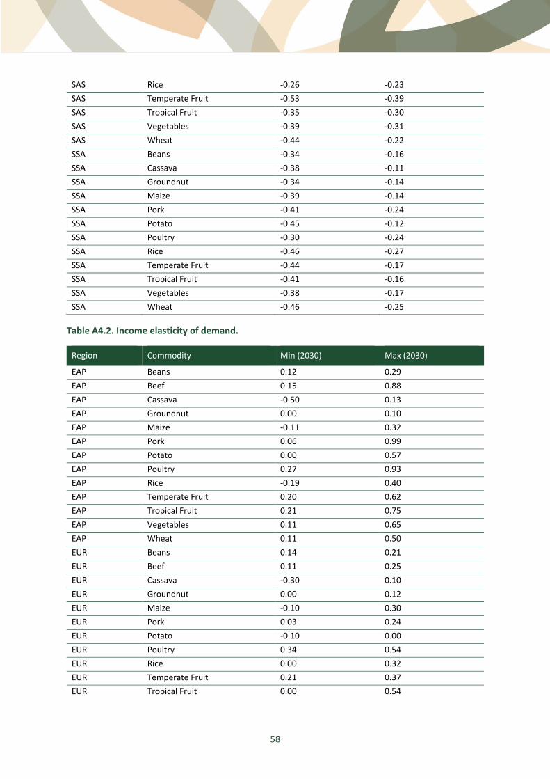
58

SAS Rice -0.26 -0.23

SAS Temperate Fruit -0.53 -0.39

SAS Tropical Fruit -0.35 -0.30

SAS Vegetables -0.39 -0.31

SAS Wheat -0.44 -0.22

SSA Beans -0.34 -0.16

SSA Cassava -0.38 -0.11

SSA Groundnut -0.34 -0.14

SSA Maize -0.39 -0.14

SSA Pork -0.41 -0.24

SSA Potato -0.45 -0.12

SSA Poultry -0.30 -0.24

SSA Rice -0.46 -0.27

SSA Temperate Fruit -0.44 -0.17

SSA Tropical Fruit -0.41 -0.16

SSA Vegetables -0.38 -0.17

SSA Wheat -0.46 -0.25

Table A4.2. Income elasticity of demand.

Region Commodity Min (2030) Max (2030)

EAP Beans 0.12 0.29

EAP Beef 0.15 0.88

EAP Cassava -0.50 0.13

EAP Groundnut 0.00 0.10

EAP Maize -0.11 0.32

EAP Pork 0.06 0.99

EAP Potato 0.00 0.57

EAP Poultry 0.27 0.93

EAP Rice -0.19 0.40

EAP Temperate Fruit 0.20 0.62

EAP Tropical Fruit 0.21 0.75

EAP Vegetables 0.11 0.65

EAP Wheat 0.11 0.50

EUR Beans 0.14 0.21

EUR Beef 0.11 0.25

EUR Cassava -0.30 0.10

EUR Groundnut 0.00 0.12

EUR Maize -0.10 0.30

EUR Pork 0.03 0.24

EUR Potato -0.10 0.00

EUR Poultry 0.34 0.54

EUR Rice 0.00 0.32

EUR Temperate Fruit 0.21 0.37

EUR Tropical Fruit 0.00 0.54

59

EUR Vegetables 0.16 0.33

EUR Wheat 0.07 0.38

FSU Beans 0.09 0.18

FSU Beef 0.05 0.45

FSU Cassava -0.31 0.10

FSU Groundnut 0.00 0.12

FSU Maize -0.10 0.10

FSU Pork 0.23 0.47

FSU Potato -0.10 0.25

FSU Poultry 0.47 0.76

FSU Rice 0.13 0.34

FSU Temperate Fruit 0.20 0.40

FSU Tropical Fruit 0.30 0.55

FSU Vegetables 0.15 0.40

FSU Wheat 0.07 0.19

LAC Beans 0.18 0.26

LAC Beef 0.06 0.61

LAC Cassava -0.20 0.10

LAC Groundnut 0.00 0.05

LAC Maize 0.02 0.17

LAC Pork 0.15 0.99

LAC Potato 0.05 0.32

LAC Poultry 0.31 0.93

LAC Rice -0.04 0.22

LAC Temperate Fruit 0.16 0.49

LAC Tropical Fruit 0.09 0.50

LAC Vegetables 0.36 0.49

LAC Wheat 0.07 0.34

MEN Beans 0.15 0.31

MEN Beef 0.03 0.72

MEN Cassava -0.20 0.10

MEN Groundnut 0.00 0.08

MEN Maize 0.00 0.31

MEN Pork -0.12 0.79

MEN Potato 0.00 0.38

MEN Poultry 0.07 0.71

MEN Rice 0.01 0.44

MEN Temperate Fruit -0.06 0.45

MEN Tropical Fruit 0.00 0.63

MEN Vegetables 0.14 0.53

MEN Wheat -0.06 0.37

NAM Beans 0.14 0.15

NAM Beef -0.03 0.03

NAM Cassava -0.31 -0.20

NAM Groundnut 0.00 0.00

60

NAM Maize 0.07 0.32

NAM Pork -0.12 0.05

NAM Potato 0.00 0.09

NAM Poultry 0.32 0.53

NAM Rice 0.09 0.43

NAM Temperate Fruit 0.24 0.36

NAM Tropical Fruit 0.28 0.37

NAM Vegetables 0.39 0.66

NAM Wheat 0.07 0.35

SAS Beans 0.13 0.27

SAS Beef 0.33 0.81

SAS Cassava -0.06 0.10

SAS Groundnut 0.00 0.06

SAS Maize 0.13 0.21

SAS Pork 0.26 0.56

SAS Potato 0.15 0.48

SAS Poultry 0.42 1.15

SAS Rice -0.14 0.19

SAS Temperate Fruit 0.46 0.87

SAS Tropical Fruit 0.39 0.95

SAS Vegetables 0.25 0.86

SAS Wheat 0.09 0.40

SSA Beans 0.14 0.30

SSA Beef 0.17 0.91

SSA Cassava -0.16 0.26

SSA Groundnut 0.00 0.17

SSA Maize -0.11 0.42

SSA Pork 0.00 1.15

SSA Potato 0.00 0.80

SSA Poultry 0.38 1.03

SSA Rice 0.02 0.68

SSA Temperate Fruit 0.11 0.78

SSA Tropical Fruit 0.13 0.92

SSA Vegetables 0.14 0.96

SSA Wheat 0.11 0.80

Table A4.3. Yield elasticity with respect to commodity price.

Region Commodity Min Max

EAP Beans 0.13 0.24

EAP Cassava 0.05 0.11

EAP Groundnut 0.07 0.12

EAP Maize 0.08 0.16

EAP Potato 0.14 0.28

EAP Rice 0.08 0.14

61

EAP Temperate Fruit 0.10 0.17

EAP Tropical Fruit 0.12 0.21

EAP Vegetables 0.13 0.45

EAP Wheat 0.10 0.17

EUR Beans 0.17 0.20

EUR Cassava 0.07 0.11

EUR Groundnut 0.08 0.10

EUR Maize 0.11 0.15

EUR Potato 0.18 0.22

EUR Rice 0.10 0.11

EUR Temperate Fruit 0.11 0.13

EUR Tropical Fruit 0.13 0.15

EUR Vegetables 0.15 0.18

EUR Wheat 0.11 0.23

FSU Beans 0.18 0.26

FSU Cassava 0.10 0.13

FSU Groundnut 0.09 0.13

FSU Maize 0.13 0.19

FSU Potato 0.20 0.30

FSU Rice 0.10 0.14

FSU Temperate Fruit 0.11 0.16

FSU Tropical Fruit 0.14 0.19

FSU Vegetables 0.16 0.23

FSU Wheat 0.11 0.16

LAC Beans 0.12 0.24

LAC Cassava 0.05 0.11

LAC Groundnut 0.06 0.12

LAC Maize 0.08 0.15

LAC Potato 0.14 0.28

LAC Rice 0.11 0.17

LAC Temperate Fruit 0.09 0.17

LAC Tropical Fruit 0.11 0.20

LAC Vegetables 0.13 0.24

LAC Wheat 0.09 0.17

MEN Beans 0.17 0.26

MEN Cassava 0.07 0.13

MEN Groundnut 0.08 0.13

MEN Maize 0.11 0.16

MEN Potato 0.20 0.32

MEN Rice 0.11 0.17

MEN Temperate Fruit 0.13 0.18

MEN Tropical Fruit 0.15 0.22

MEN Vegetables 0.18 0.47

MEN Wheat 0.13 0.18

NAM Beans 0.18 0.23

62

NAM Cassava 0.07 0.11

NAM Groundnut 0.09 0.11

NAM Maize 0.16 0.21

NAM Potato 0.20 0.26

NAM Rice 0.11 0.13

NAM Temperate Fruit 0.12 0.14

NAM Tropical Fruit 0.14 0.17

NAM Vegetables 0.17 0.20

NAM Wheat 0.12 0.14

SAS Beans 0.22 0.28

SAS Cassava 0.10 0.13

SAS Groundnut 0.11 0.14

SAS Maize 0.13 0.17

SAS Potato 0.26 0.32

SAS Rice 0.10 0.14

SAS Temperate Fruit 0.16 0.20

SAS Tropical Fruit 0.19 0.24

SAS Vegetables 0.22 0.52

SAS Wheat 0.16 0.25

SSA Beans 0.22 0.32

SSA Cassava 0.11 0.16

SSA Groundnut 0.11 0.16

SSA Maize 0.13 0.20

SSA Potato 0.26 0.38

SSA Rice 0.13 0.21

SSA Temperate Fruit 0.14 0.23

SSA Tropical Fruit 0.17 0.27

SSA Vegetables 0.20 0.32

SSA Wheat 0.14 0.23

Table A4.4. Yield elasticity with respect to input prices.

Region Commodity Min of FERT Max of FERT Min of wage Max of wage

EAP Beans -0.10 -0.01 -0.09 -0.01

EAP Cassava -0.05 -0.03 -0.09 -0.02

EAP Groundnut -0.10 -0.01 -0.09 -0.01

EAP Maize -0.06 -0.03 -0.11 -0.02

EAP Potato -0.05 -0.03 -0.11 -0.02

EAP Rice -0.06 -0.03 -0.10 -0.02

EAP Temperate Fruit -0.06 0.00 -0.06 -0.01

EAP Tropical Fruit -0.07 0.00 -0.07 -0.01

EAP Vegetables -0.08 0.00 -0.08 -0.01

EAP Wheat -0.06 -0.03 -0.12 -0.02

EUR Beans -0.07 -0.02 -0.07 -0.01

EUR Cassava -0.04 -0.03 -0.08 -0.03

63

EUR Groundnut -0.07 -0.02 -0.07 -0.01

EUR Maize -0.06 -0.04 -0.09 -0.04

EUR Potato -0.05 -0.03 -0.08 -0.03

EUR Rice -0.05 -0.04 -0.07 -0.03

EUR Temperate Fruit -0.04 -0.02 -0.04 -0.02

EUR Tropical Fruit -0.05 -0.02 -0.05 -0.02

EUR Vegetables -0.06 -0.03 -0.06 -0.02

EUR Wheat -0.05 -0.04 -0.08 -0.03

FSU Beans -0.07 -0.02 -0.10 -0.03

FSU Cassava -0.04 -0.03 -0.10 -0.08

FSU Groundnut -0.07 -0.02 -0.10 -0.03

FSU Maize -0.06 -0.04 -0.13 -0.08

FSU Potato -0.04 -0.03 -0.11 -0.07

FSU Rice -0.05 -0.04 -0.10 -0.07

FSU Temperate Fruit -0.03 -0.02 -0.06 -0.04

FSU Tropical Fruit -0.03 -0.02 -0.07 -0.04

FSU Vegetables -0.04 -0.03 -0.08 -0.05

FSU Wheat -0.05 -0.04 -0.11 -0.07

LAC Beans -0.04 -0.03 -0.08 -0.03

LAC Cassava -0.03 -0.03 -0.09 -0.03

LAC Groundnut -0.04 -0.03 -0.08 -0.03

LAC Maize -0.05 -0.04 -0.10 -0.04

LAC Potato -0.04 -0.04 -0.11 -0.04

LAC Rice -0.05 -0.04 -0.11 -0.04

LAC Temperate Fruit -0.03 -0.02 -0.06 -0.02

LAC Tropical Fruit -0.04 -0.03 -0.07 -0.03

LAC Vegetables -0.05 -0.03 -0.08 -0.03

LAC Wheat -0.06 -0.04 -0.11 -0.04

MEN Beans -0.10 -0.01 -0.12 -0.02

MEN Cassava -0.05 -0.03 -0.13 -0.05

MEN Groundnut -0.10 -0.01 -0.12 -0.02

MEN Maize -0.06 -0.03 -0.14 -0.05

MEN Potato -0.05 -0.03 -0.14 -0.05

MEN Rice -0.06 -0.03 -0.14 -0.05

MEN Temperate Fruit -0.05 -0.01 -0.08 -0.03

MEN Tropical Fruit -0.05 -0.01 -0.10 -0.03

MEN Vegetables -0.06 -0.01 -0.11 -0.04

MEN Wheat -0.06 -0.03 -0.16 -0.05

NAM Beans -0.10 -0.08 -0.02 -0.01

NAM Cassava -0.05 -0.03 -0.05 -0.01

NAM Groundnut -0.10 -0.08 -0.02 -0.01

NAM Maize -0.05 -0.03 -0.06 -0.01

NAM Potato -0.05 -0.03 -0.05 -0.01

NAM Rice -0.05 -0.03 -0.05 -0.01

NAM Temperate Fruit -0.05 -0.05 -0.03 -0.01

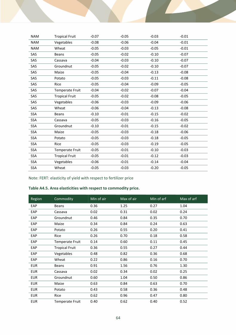
64

NAM Tropical Fruit -0.07 -0.05 -0.03 -0.01

NAM Vegetables -0.08 -0.06 -0.04 -0.01

NAM Wheat -0.05 -0.03 -0.05 -0.01

SAS Beans -0.05 -0.02 -0.10 -0.07

SAS Cassava -0.04 -0.03 -0.10 -0.07

SAS Groundnut -0.05 -0.02 -0.10 -0.07

SAS Maize -0.05 -0.04 -0.13 -0.08

SAS Potato -0.05 -0.03 -0.11 -0.08

SAS Rice -0.05 -0.04 -0.09 -0.05

SAS Temperate Fruit -0.04 -0.02 -0.07 -0.04

SAS Tropical Fruit -0.05 -0.02 -0.08 -0.05

SAS Vegetables -0.06 -0.03 -0.09 -0.06

SAS Wheat -0.06 -0.04 -0.13 -0.08

SSA Beans -0.10 -0.01 -0.15 -0.02

SSA Cassava -0.05 -0.03 -0.16 -0.05

SSA Groundnut -0.10 -0.01 -0.15 -0.02

SSA Maize -0.05 -0.03 -0.18 -0.06

SSA Potato -0.05 -0.03 -0.18 -0.05

SSA Rice -0.05 -0.03 -0.19 -0.05

SSA Temperate Fruit -0.05 -0.01 -0.10 -0.03

SSA Tropical Fruit -0.05 -0.01 -0.12 -0.03

SSA Vegetables -0.06 -0.01 -0.14 -0.04

SSA Wheat -0.05 -0.03 -0.20 -0.05

Note: FERT: elasticity of yield with respect to fertilizer price

Table A4.5. Area elasticities with respect to commodity price.

Region Commodity Min of air Max of air Min of arf Max of arf

EAP Beans 0.36 1.25 0.27 1.04

EAP Cassava 0.02 0.31 0.02 0.24

EAP Groundnut 0.46 0.84 0.35 0.70

EAP Maize 0.34 0.84 0.24 0.63

EAP Potato 0.26 0.55 0.20 0.41

EAP Rice 0.26 0.70 0.18 0.58

EAP Temperate Fruit 0.14 0.60 0.11 0.45

EAP Tropical Fruit 0.36 0.55 0.27 0.44

EAP Vegetables 0.48 0.82 0.36 0.68

EAP Wheat 0.22 0.86 0.16 0.70

EUR Beans 0.91 1.56 0.76 1.30

EUR Cassava 0.02 0.34 0.02 0.25

EUR Groundnut 0.60 1.04 0.50 0.86

EUR Maize 0.63 0.84 0.63 0.70

EUR Potato 0.43 0.58 0.36 0.48

EUR Rice 0.62 0.96 0.47 0.80

EUR Temperate Fruit 0.40 0.62 0.40 0.52

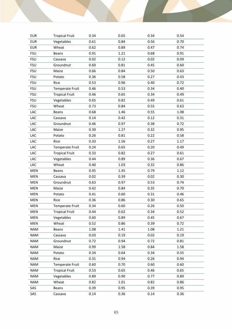
65

EUR Tropical Fruit 0.34 0.65 0.34 0.54

EUR Vegetables 0.61 0.84 0.56 0.70

EUR Wheat 0.62 0.89 0.47 0.74

FSU Beans 0.91 1.21 0.68 0.91

FSU Cassava 0.02 0.12 0.02 0.09

FSU Groundnut 0.60 0.81 0.45 0.60

FSU Maize 0.66 0.84 0.50 0.63

FSU Potato 0.36 0.58 0.27 0.43

FSU Rice 0.53 0.96 0.40 0.72

FSU Temperate Fruit 0.46 0.53 0.34 0.40

FSU Tropical Fruit 0.46 0.65 0.34 0.49

FSU Vegetables 0.65 0.82 0.49 0.61

FSU Wheat 0.73 0.84 0.55 0.63

LAC Beans 0.68 1.46 0.55 1.08

LAC Cassava 0.14 0.42 0.12 0.31

LAC Groundnut 0.46 0.97 0.38 0.72

LAC Maize 0.39 1.27 0.32 0.95

LAC Potato 0.26 0.81 0.22 0.58

LAC Rice 0.33 1.56 0.27 1.17

LAC Temperate Fruit 0.24 0.65 0.20 0.49

LAC Tropical Fruit 0.33 0.82 0.27 0.61

LAC Vegetables 0.44 0.89 0.36 0.67

LAC Wheat 0.40 1.03 0.32 0.86

MEN Beans 0.95 1.45 0.79 1.12

MEN Cassava 0.02 0.39 0.02 0.30

MEN Groundnut 0.63 0.97 0.53 0.74

MEN Maize 0.42 0.84 0.35 0.70

MEN Potato 0.41 0.60 0.31 0.46

MEN Rice 0.36 0.86 0.30 0.65

MEN Temperate Fruit 0.34 0.60 0.26 0.50

MEN Tropical Fruit 0.44 0.62 0.34 0.52

MEN Vegetables 0.60 0.89 0.45 0.67

MEN Wheat 0.52 0.86 0.39 0.72

NAM Beans 1.08 1.41 1.08 1.21

NAM Cassava 0.03 0.19 0.02 0.19

NAM Groundnut 0.72 0.94 0.72 0.81

NAM Maize 0.99 1.58 0.84 1.58

NAM Potato 0.34 0.64 0.34 0.55

NAM Rice 0.31 0.94 0.26 0.94

NAM Temperate Fruit 0.60 0.70 0.60 0.60

NAM Tropical Fruit 0.53 0.65 0.46 0.65

NAM Vegetables 0.89 0.90 0.77 0.89

NAM Wheat 0.82 1.01 0.82 0.86

SAS Beans 0.39 0.95 0.39 0.95

SAS Cassava 0.14 0.36 0.14 0.36

66

SAS Groundnut 0.49 0.63 0.37 0.63

SAS Maize 0.29 0.87 0.22 0.87

SAS Potato 0.41 0.58 0.36 0.58

SAS Rice 0.43 0.64 0.32 0.62

SAS Temperate Fruit 0.36 0.43 0.27 0.43

SAS Tropical Fruit 0.41 0.53 0.36 0.53

SAS Vegetables 0.48 0.62 0.36 0.62

SAS Wheat 0.43 0.65 0.32 0.65

SSA Beans 0.55 1.90 0.55 1.12

SSA Cassava 0.02 0.55 0.02 0.36

SSA Groundnut 0.38 1.27 0.38 0.74

SSA Maize 0.28 1.16 0.32 0.73

SSA Potato 0.22 0.84 0.22 0.46

SSA Rice 0.24 0.91 0.18 0.63

SSA Temperate Fruit 0.20 0.70 0.20 0.52

SSA Tropical Fruit 0.27 0.95 0.27 0.52

SSA Vegetables 0.36 1.31 0.36 0.72

SSA Wheat 0.32 1.22 0.32 0.67

Note: air: irrigated crops; arf: rainfed crops.

The Commission on Sustainable Agriculture

Intensification (CoSAI) brings together 21

Commissioners to influence public and private

support to innovation in order to rapidly scale

up sustainable agricultural intensification (SAI) in

the Global South.

For CoSAI, innovation means the development

and uptake of new ways of doing things – in

policy, social institutions and finance, as well as

in science and technology.

Contact us: [email protected]

wle.cgiar.org/cosai

https://wle.cgiar.org/cosai/

https://wle.cgiar.org/cosai/

mailto:[email protected]

Documents

Estimating the Global Investment Gap in Research and