WP/15/144

IMF Working Papers describe research in progress by the author(s) and are published to elicit comments and to encourage debate. The views expressed in IMF Working Papers are those of the author(s) and do not necessarily represent the views of the IMF, its Executive Board, or IMF management.

A New Methodology for Estimating the Output Gap in the United States

by Ali Alichi

IMF Working Paper

Western Hemisphere Department

A New Methodology for Estimating the Output Gap in the United States

Prepared by Ali Alichi

Authorized for distribution by Nigel Chalk

July 2015

Abstract

The gap between potential and actual output—the output gap—is a key variable for

policymaking. This paper adapts the methodology developed in Blagrave and others (2015) to

estimate the path of output gap in the U.S. economy. The results show that the output gap has

considerably shrunk since the Great Recession, but still remains negative. While the results are

more robust than other existing methodologies, there is still significant uncertainty surrounding

the estimates.

JEL Classification Numbers: C51, E31, E52

Keywords: Macroeconomic Modeling, Potential Output, Output Gap

Author’s E-Mail Address: aalichi@imf.org

IMF Working Papers describe research in progress by the author(s) and are published to

elicit comments and to encourage debate. The views expressed in IMF Working Papers are

those of the author(s) and do not necessarily represent the views of the IMF, its Executive Board,

or IMF management.

WP/15/144© 2015 International Monetary Fund

2

Contents

I. Introduction ______________________________________________________________3

II. Definitions ______________________________________________________________4

III. Existing Methodologies ___________________________________________________4

IV. Methodology ____________________________________________________________6

V. Results ________________________________________________________________11

VI. Dealing with the End-of-Sample Problem ____________________________________12

VII. Conclusion ____________________________________________________________13

References ________________________________________________________________14

Appendix I: Estimation Results _______________________________________________16

Appendix II: Labor Force Participation Projections ________________________________16

3

I. INTRODUCTION

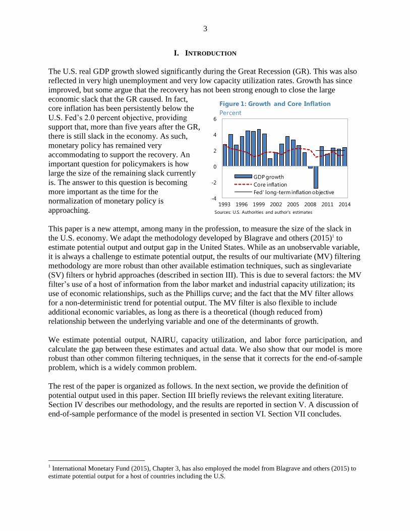
The U.S. real GDP growth slowed significantly during the Great Recession (GR). This was also

reflected in very high unemployment and very low capacity utilization rates. Growth has since

improved, but some argue that the recovery has not been strong enough to close the large

economic slack that the GR caused. In fact,

core inflation has been persistently below the

U.S. Fed’s 2.0 percent objective, providing

support that, more than five years after the GR,

there is still slack in the economy. As such,

monetary policy has remained very

accommodating to support the recovery. An

important question for policymakers is how

large the size of the remaining slack currently

is. The answer to this question is becoming

more important as the time for the

normalization of monetary policy is

approaching.

This paper is a new attempt, among many in the profession, to measure the size of the slack in

the U.S. economy. We adapt the methodology developed by Blagrave and others (2015)1 to

estimate potential output and output gap in the United States. While as an unobservable variable,

it is always a challenge to estimate potential output, the results of our multivariate (MV) filtering

methodology are more robust than other available estimation techniques, such as singlevariate

(SV) filters or hybrid approaches (described in section III). This is due to several factors: the MV

filter’s use of a host of information from the labor market and industrial capacity utilization; its

use of economic relationships, such as the Phillips curve; and the fact that the MV filter allows

for a non-deterministic trend for potential output. The MV filter is also flexible to include

additional economic variables, as long as there is a theoretical (though reduced from)

relationship between the underlying variable and one of the determinants of growth.

We estimate potential output, NAIRU, capacity utilization, and labor force participation, and

calculate the gap between these estimates and actual data. We also show that our model is more

robust than other common filtering techniques, in the sense that it corrects for the end-of-sample

problem, which is a widely common problem.

The rest of the paper is organized as follows. In the next section, we provide the definition of

potential output used in this paper. Section III briefly reviews the relevant exiting literature.

Section IV describes our methodology, and the results are reported in section V. A discussion of

end-of-sample performance of the model is presented in section VI. Section VII concludes.

1 International Monetary Fund (2015), Chapter 3, has also employed the model from Blagrave and others (2015) to

estimate potential output for a host of countries including the U.S.

-4

-2

0

2

4

6

1993 1996 1999 2002 2005 2008 2011 2014

GDP growth

Core inflation

Fed' long-term inflation objective

Figure 1: Growth and Core Inflation

Percent

Sources: U.S. Authorities and author's estimates

4

II. DEFINITIONS

In this paper, potential output is defined as the level of output that can be achieved without

giving any upside or downside pressures on inflation. This definition is based on Okun (1962)

and is widely used in the literature. The output gap is defined as the difference between the

actual and potential output in percent of potential output. When the output gap is zero, there is no

upward or downward pressure on inflation, as actual demand coincides with economy’s

potential. Shocks can affect actual output and potential output differently, leading to non-zero

output gap levels. If the output gap is positive, so that actual output is greater than potential

output, inflation will begin to rise in response to demand pressures. Similarly, if the output gap is

negative, so that actual output falls below potential output, prices will begin to fall to reflect

weak demand. An important feature of this paper is that, macroeconomic shocks are not

exclusive to the actual output; potential can also be hit by shocks. In other words, the path of

potential output is not deterministic. This is in contrast to many contributions in the literature,

some of which we briefly review below.

III. EXISTING METHODOLOGIES

All commonly used methodologies to estimate the potential output involve filtering of the

macroeconomic data to extract the unobservable underlying potential output level from cyclical

variations in the output.

Singlevariate and hybrid approaches

The simplest methodology to estimate potential output is the singlevariate (SV) filter. This is a

purely statistical methodology, which filters the actual GDP data to extract the trend as its

estimate of potential output. The most common SV filter is the Hodrick-Prescott (HP) filter. It is

very easy to use the HP filter because it only requires one data series (output). However, for the

same reason, the HP filter is not a reliable technique for estimating potential: it does not take

advantage of information from other economic data, say inflation or labor market indicators, to

guide its estimate of potential output. There are other technical problems with the HP filter too,

the most import of which is the end-of sample problem, with estimates towards the end of a

given sample period being subject to significant revisions as more data ultimately become

available and the sample is extended.

Another technique to estimate potential output is the “hybrid” approach. It uses a SV filter to

estimate trend labor and total factor productivity (TFP) and combines them with capital stock

through an assumed production function to arrive at potential output. The Congressional Budget

Office (2001) provides a detailed account of such a hybrid model, in which the methodology is

applied to different sectors of the U.S. economy. This approach is richer than a SV filter because

it allows for more detailed examination of the drivers of potential. A downside of this approach

is that it assumes capital is always at its potential. The hybrid approach also suffers from the end-

of-sample problems. In addition, neither the hybrid approach nor the SV filter necessarily

produce estimates of potential, which are consistent with the definition of the level giving no

pressure for inflation rise or fall as they fail to necessarily adjust for variations in inflation in

their estimates.

5

Both the SV filter and the hybrid approach also suffer from the potential misspecification by

assuming a deterministic trend. In other words, trend potential output is not allowed to respond

to shocks that could raise or lower potential over time. This is problematic, especially when the

economy is hit by a large real shock such as during the GR.

MV filter

Many contributions have adopted MV filtering methodologies to estimate potential output. Some

examples are models of Laxton and Tetlow (1992), Kuttner (1994), Benes and others (2010),

Fleischman and Roberts (2011), and Blagrave and others (2015). MV filtering involves

separating potential output from cyclical fluctuations, through the use of data and relationships

between output and other macroeconomic variables, such as inflation, labor market indicators,

capital formation indicators, etc. This approach adds economic structure to estimates by

conditioning them on some basic theoretical relationships (such as a Phillip’s curve relating the

inflation process to the output gap). MV filtering methodologies are more complicated than SV

filtering methodologies and require more data, but are at the same time more reliable because

they use more information from the data for their estimates.

Shortcomings of the MV filtering approach are similar to those facing other methods—there

remains an end-of-sample problem, (although we have addressed it largely in this paper using the

information from growth and inflation expectations) and the estimates of potential and the output

gap are only improved relative to a simple statistical filtration if the structural relationships

specified in the filter are valid ones.

The MV filtering approach has the advantage of imposing well-known empirical relationships. In

particular, the MV filtering approach adopted in this paper ensures that estimates of the output

gap and potential are consistent with the Okun definition of potential. In addition, in its simplest

form, this technique is relatively easy to implement requiring only a few variables, and it can

also be augmented where data availability permits.

DSGE models

Some contributions have used DSGE models to estimate potential and the output gap (see, for

example, Vetlov and others, 2011). These models have more tangible micro foundations and are

very appealing. Nonetheless, these they are not so easy to interpret and remain a challenge for

policymakers to use in formulation of policies.

Other models

While most contributions, including this paper, have a closed-economy model, some recent work

has focused on an open economy case. For example, Alberoa and others (2013) have expanded

the definition of potential output to include global imbalances. Yet, another recent strand of

literature is focusing on including financial imbalances in the definition of the potential output

(see Borio, Disyatat, and Juselius (2013)).

6

IV. METHODOLOGY

The MV filtering approach specified in this paper is an extension of Blagrave and others (2015).

In addition to real GDP growth, core PCE inflation, and the unemployment rate, we introduce

new blocks to introduce capacity utilization and labor market participation rate in the model.

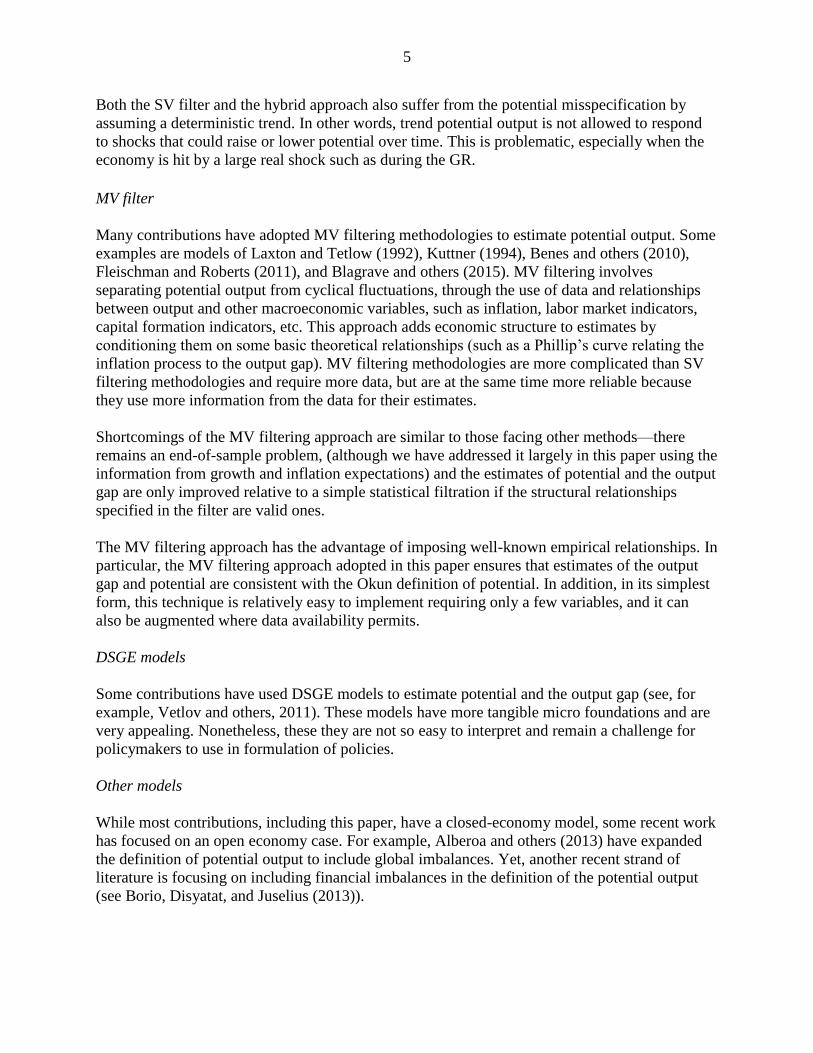
Inclusion of capacity utilization is crucial to have a reliable measure of potential output.2

Figure 2 shows that in the second half of 1990s, capacity utilization and the unemployment rate

were both declining, with opposite implications for potential growth. 3 Hence, just relying on

labor market data could be misleading for projecting potential. The decline in the unemployment

rate is consistent with an improving potential output growth, while a decline in the capacity

utilization likely leads to lower potential output growth. Ignoring the capacity utilization and

only relying on the unemployment rate, therefore, results in overestimating potential output and

underestimating the path of the output gap, in the later years.

We specify reduced-formed relationships between these observable variables and some latent

variables that we introduce in the model.

2 The new block on labor force participation rate also enriches the model, but we do not see it as crucial as the block

on capacity utilization. This is because the original model already included another labor market block (on

unemployment rate.)

3 Analyzing why capacity utilization has been declining since 1990 is beyond the scope of this paper.

60

70

80

90

3

6

9

12

1993 1996 1999 2002 2005 2008 2011 2014

Unemployment rate

Capacity utilization (RHS)

Figure 2: Unemployment and Capacity

Utilization (percent)

Sources: U.S. Authorities and author's estimates

7

Model

The output gap is defined as the deviation of real GDP, in log terms ( ), from its potential level

( ):

(1)

The stochastic process for output (real GDP) is comprised of three equations, and subject to three

types of shocks. First, the level of potential output ( evolves according to potential growth

( and a level-shock term ( :

(2)

Potential growth is also subject to shocks ( ), with their impact fading gradually according to

the parameter (with lower values entailing a slower adjustment back to the steady-state growth

rate following a shock):

(3)

Finally, the output gap closes over time at a speed pinned down by parameter ( ), but is also

subject to demand shocks ( :

(4)

In the absence of any shocks, output would be at its steady state path and the output gap would

be zero. Shocks can be threefold. They occur to: the level of potential ( ); the growth rate of

potential ( ); or the output gap (

), and can cause output to deviate from this initial steady-

state path over time. Output is assumed to always return to its steady-state path following any

shocks. A shock to the level of potential output in any given period will cause output to be

permanently higher (or lower) than its initial steady-state path. Similarly, shocks to the growth

rate of potential can cause the growth rate of output to be temporarily higher, before ultimately

slowing back to the steady-state growth rate (note that this would still entail a higher level of

output). And, finally, shocks to the output gap cause only a temporary deviation of output from

potential.

In order to identify the three aforementioned output shock terms, a Phillips curve equation for

inflation is added, which links the evolution of the output gap (an unobservable variable) to

observable data on inflation according to the process. The Phillips curve equation is as follows:4

(5)

4 This non-linear form is only used for projections. For historical Bayesian estimation, a linear equation (

) has been used, given that we do not have at our disposal a non-linear

estimation technique. The nonlinearity does not make a notable difference in the results, unless the output gap is

large and positive.

8

Equations describing the evolution of unemployment are further included to provide additional

identifying information for the estimation of the output gap. The first three of these equations (6-

8) are similar to the equations presented above for output. The unemployment gap ( ) is defined

in equation 6, as the difference between the actual unemployment rate ( ) and NAIRU ( ):

(6)

NAIRU converges to its steady state level (

), which is determined outside the model, but also

has a time varying trend ( ) and can experience shocks as well ( ):

(7)

The time varying portion of NAIRU, reflects gradually increased dynamism over time, due to

improved information sharing and easier mobility of the labor force, but could experience shocks

( ):

(8)

The last equation of the labor market block is an Okun’s rule equation, in which the

unemployment gap depends on its past value and the output gap, but it also can experience

shocks ( ):

(9)

One important aspect of the U.S. labor market is the effect of aging on labor participation and

hence the unemployment rate. The following set of equations is intended to capture this

important dynamic. Equation 10 defines the labor force participation gap as the difference

between labor force participation ( ) and potential labor force participation ( ):

(10)

Potential labor force participation converges to its steady state (

), absent any shocks ( ):

(11)

Labor force participation gap depends on its lagged value and the unemployment gap, but can

also experience shocks (

):

(12) +

Next, equations describing the evolution of capacity utilization provide further identifying

information. In equation 13, capacity utilization gap ( ) is defined as the difference of

capacity utilization ( ) and its potential level ( ) at each period:

(13)

9

Potential capacity utilization converges to its steady state level (

) over time, but could

also experience shocks:

(14)

The last equation for the capacity utilization block is in the spirit of an Okun’s rule, but for

capacity utilization. Capacity utilization gap depends on its lag, the output gap, but it can also

experience shocks (

):

(15) +

Next, we add equations that enable us to use information from growth and inflation expectations

data. These equations capture the assumptions that expectations are formed rationally and

fulfilled in the longer term, but do not materialize exactly in the short term, modeled with

shocks:

(16)

, j = 0,…,5

(17)

, j = 0,1

Where ( ) and ( ) are expected and actual model-consistent GDP growth rates in j periods

ahead, respectively. The difference between the two is captured by a shock term (

).

Likewise, ( ) and ( ) are expected and actual model-consistent core PCE inflation rates in

j periods ahead, respectively. The difference between the two is captured by a shock term (

).

Data for growth and inflation expectation are from Consensus Economics. The ‘strength’ of the

relationship between the data on consensus and the model’s forward expectations is determined

by the standard deviation of the error terms. In practice, the estimated variance of these terms

allows consensus data to influence, but not completely override, the model’s expectations,

particularly at the end of the sample period. The incorporation of consensus forecasts can be

thought as a heuristic approach to blend forecasts from different sources and methods. The

resulting impact of this information on the historical estimates of potential and the output gap is

modest, as shown in the following section.

We use annual data for observables (GDP, PCE inflation, unemployment rate, labor force

participation, and capacity utilization) from the U.S. authorities and other variables in the model

are unobservable. We estimate the model with Bayesian estimation techniques. This is what is

generally referred to as Kalman filtering techniques.5

5 See Hamilton (1994) for a more detailed discussion of the Kalman filter, which is used to obtain estimates of the

unobservable variables as part of the estimation process.

10

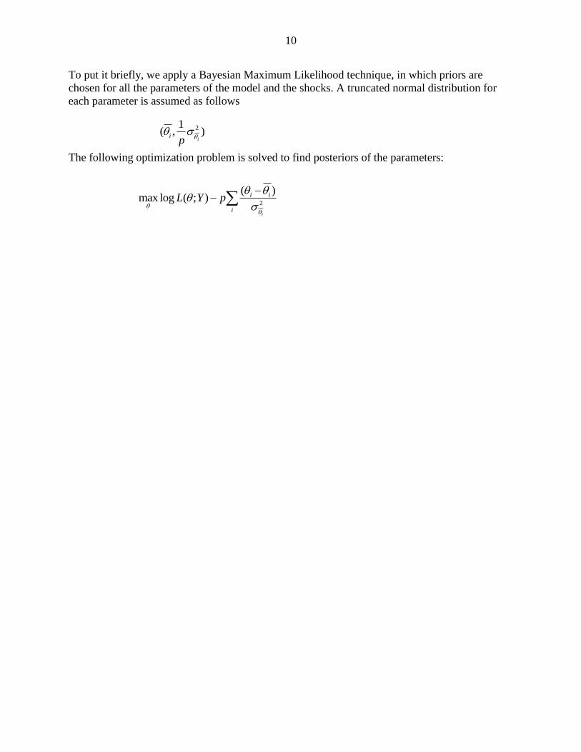
To put it briefly, we apply a Bayesian Maximum Likelihood technique, in which priors are

chosen for all the parameters of the model and the shocks. A truncated normal distribution for

each parameter is assumed as follows

The following optimization problem is solved to find posteriors of the parameters:

21( , )

ii

p

2

( )max log ( ; )

i

i i

i

L Y p

11

-8

-6

-4

-2

0

2

4

1993 1996 1999 2002 2005 2008 2011 2014 2017 2020

Output gapUnemployment gapCapacity utilization gap

Figure 6: Output, Unemployment, and

Capacity Util. Gaps (percent of potential)

Source: Author's estimates

V. RESULTS

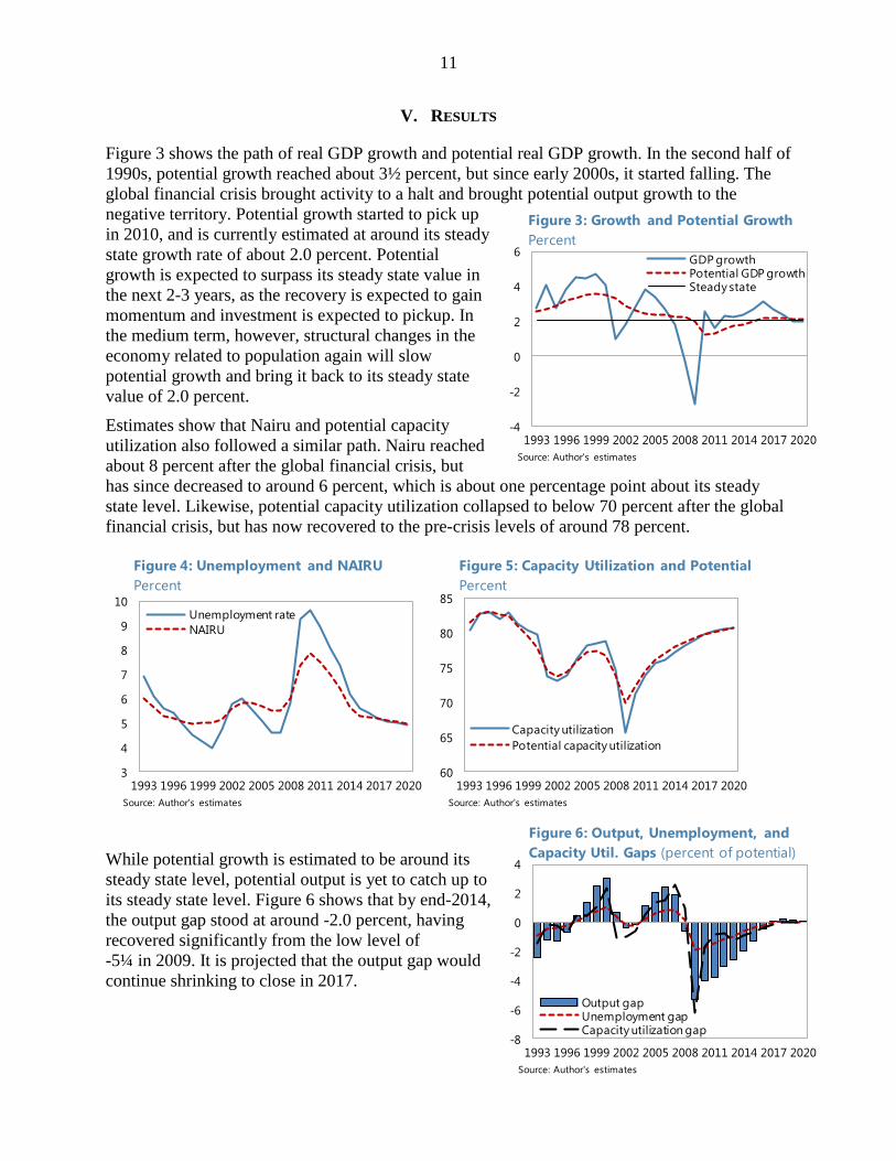
Figure 3 shows the path of real GDP growth and potential real GDP growth. In the second half of

1990s, potential growth reached about 3½ percent, but since early 2000s, it started falling. The

global financial crisis brought activity to a halt and brought potential output growth to the

negative territory. Potential growth started to pick up

in 2010, and is currently estimated at around its steady

state growth rate of about 2.0 percent. Potential

growth is expected to surpass its steady state value in

the next 2-3 years, as the recovery is expected to gain

momentum and investment is expected to pickup. In

the medium term, however, structural changes in the

economy related to population again will slow

potential growth and bring it back to its steady state

value of 2.0 percent.

Estimates show that Nairu and potential capacity

utilization also followed a similar path. Nairu reached

about 8 percent after the global financial crisis, but

has since decreased to around 6 percent, which is about one percentage point about its steady

state level. Likewise, potential capacity utilization collapsed to below 70 percent after the global

financial crisis, but has now recovered to the pre-crisis levels of around 78 percent.

While potential growth is estimated to be around its

steady state level, potential output is yet to catch up to

its steady state level. Figure 6 shows that by end-2014,

the output gap stood at around -2.0 percent, having

recovered significantly from the low level of

-5¼ in 2009. It is projected that the output gap would

continue shrinking to close in 2017.

3

4

5

6

7

8

9

10

1993 1996 1999 2002 2005 2008 2011 2014 2017 2020

Unemployment rate

NAIRU

Figure 4: Unemployment and NAIRU

Percent

Source: Author's estimates

60

65

70

75

80

85

1993 1996 1999 2002 2005 2008 2011 2014 2017 2020

Capacity utilization

Potential capacity utilization

Figure 5: Capacity Utilization and Potential

Percent

Source: Author's estimates

-4

-2

0

2

4

6

1993 1996 1999 2002 2005 2008 2011 2014 2017 2020

GDP growthPotential GDP growthSteady state

Figure 3: Growth and Potential Growth

Percent

Source: Author's estimates

12

VI. DEALING WITH THE END-OF-SAMPLE PROBLEM

A well known problem with filters is the end-of-sample problem. Recall that

the optimization problem that, say, an HP filter solves is through trading off the size of

deviations from trend and the smoothness of that trend. Consider a postive temporary shock to

output. This would not result in a sizable change in the trend since this implies raising the trend

before the shock and lowering it afterwards. At the end of the sample, however, there is no

penalty, implying that the optimal trend will be more responsive to temporary shocks at the end

of sample than in middle of the sample. MV filters are also generally subject to this end-of-

sample problem. However, in our MV filter, this issue has been largely resolved through using

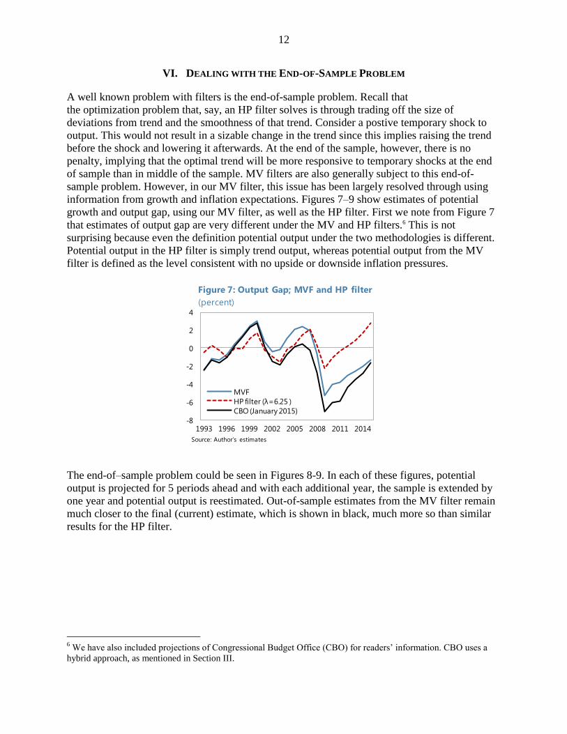
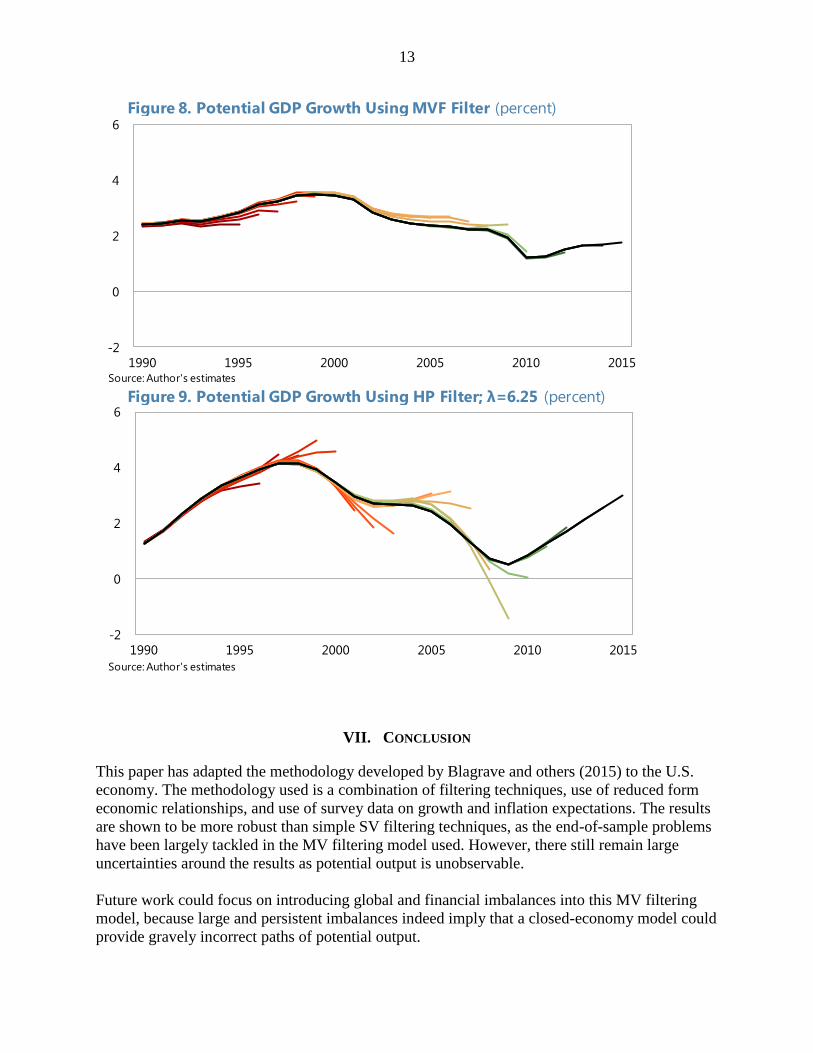
information from growth and inflation expectations. Figures 7–9 show estimates of potential

growth and output gap, using our MV filter, as well as the HP filter. First we note from Figure 7

that estimates of output gap are very different under the MV and HP filters.6 This is not

surprising because even the definition potential output under the two methodologies is different.

Potential output in the HP filter is simply trend output, whereas potential output from the MV

filter is defined as the level consistent with no upside or downside inflation pressures.

The end-of–sample problem could be seen in Figures 8-9. In each of these figures, potential

output is projected for 5 periods ahead and with each additional year, the sample is extended by

one year and potential output is reestimated. Out-of-sample estimates from the MV filter remain

much closer to the final (current) estimate, which is shown in black, much more so than similar

results for the HP filter.

6 We have also included projections of Congressional Budget Office (CBO) for readers’ information. CBO uses a

hybrid approach, as mentioned in Section III.

-8

-6

-4

-2

0

2

4

1993 1996 1999 2002 2005 2008 2011 2014

MVF

HP filter (λ=6.25 )

CBO (January 2015)

Figure 7: Output Gap; MVF and HP filter

(percent)

Source: Author's estimates

13

VII. CONCLUSION

This paper has adapted the methodology developed by Blagrave and others (2015) to the U.S.

economy. The methodology used is a combination of filtering techniques, use of reduced form

economic relationships, and use of survey data on growth and inflation expectations. The results

are shown to be more robust than simple SV filtering techniques, as the end-of-sample problems

have been largely tackled in the MV filtering model used. However, there still remain large

uncertainties around the results as potential output is unobservable.

Future work could focus on introducing global and financial imbalances into this MV filtering

model, because large and persistent imbalances indeed imply that a closed-economy model could

provide gravely incorrect paths of potential output.

-2

0

2

4

6

1990 1995 2000 2005 2010 2015

Figure 8. Potential GDP Growth Using MVF Filter (percent)

Source: Author's estimates

-2

0

2

4

6

1990 1995 2000 2005 2010 2015

Figure 9. Potential GDP Growth Using HP Filter; λ=6.25 (percent)

Source: Author's estimates

14

References

Aguiar, M., and G. Gopinath, 2007, “Emerging Market Business Cycles: The Cycle Is the

Trend”, Journal of Political Economy, University of Chicago Press, vol. 115, pp. 69-102

Alberoa, E., A. Estrada, and D. Santabarbara, 2013, “Growth Beyond Imbalances. Sustainable

Growth Rates and Output Gap Reassessment,” Banco de Espana Documentos de Trabajo

no. 1313

Bank of Canada, 2009, Monetary Policy Report, July 2009.

http://www.bankofcanada.ca/wp-content/uploads/2010/04/mpr230709.pdf

Bank of Canada, 2014, Monetary Policy Report, October 2014.

http://www.bankofcanada.ca/wp-content/uploads/2014/07/mpr-2014-10-22.pdf

Barnett, R., S. Kozicki, and C. Petrinec, 2009, “Parsing Shocks: Real-Time Revisions to Gap and

Growth Projections for Canada,” Federal Reserve Bank of St. Louis Review, pp. 247-

265.

Benes, J., K. Clinton, R. Garcia-Saltos, M. Johnson, D. Laxton, P. Manchev, and T. Matheson,

2010, “Estimating Potential Output with a Multivariate Filter,” IMF Working Paper

WP/10/285.

Benes, J., M. Kumhof, and D. Laxton. 2014, “Financial Crises in DSGE Models: Selected

Applications of MAPMOD.” Working Paper 14/56, International Monetary Fund,

Washington.

Benes, J., M. Kumhof, and D. Laxton. 2014, “Financial Crises in DSGE Models: A Prototype

Model.” Working Paper 14/57, International Monetary Fund, Washington.

Benes, J., and P. N’Diaye, 2004, “A Multivariate Filter for Measuring Potential Output and the

NAIRU: Application to The Czech Republic,” IMF Working Paper WP/04/45.

Blagrave, P., R. Garcia-Saltos, D. Laxton, and F. Zhang, “A Simple Multivariate Filter for

Estimating Potential Output,” IMF Working Paper WP/15/79.

Borio, C., P. Disyatat, and M. Juselius, 2013, “Rethinking Potential Output: Embedding

Information about the Financial Cycle,” BIS Working paper no. 404.

Butler, L., 1996, “The Bank of Canada’s New Quarterly Projection Model, Part 4. A Semi-

Structural Method to Estimate Potential Output: Combining Economic Theory with a

Time-Series Filter,” Technical Report no. 77 (Ottawa: Bank of Canada).

Cotis, JP, J. Elmeskov, and A. Mourougane, 2004, “Estimates of Potential Output: Benefits and

Pitfalls from a Policy Perspective.” Published in Euro Area Business Cycle: Stylized

Facts and Measurement Issues, pp. 35-60.

15

D’Auria, F, C. Denis, K. Havik, K. McMorrow, C. Planas, R. Raciborski, W. Roger, A. Rossi,

2010, “The production function methodology for calculating potential growth rates and

output gaps” European Commission Economic Papers No 420, July 2010.

De Masi, P. R., 1997, “IMF Estimates of Potential Output: Theory and Practice,” IMF Working

Paper WP/97/177.

Fleischman, C., and J. M. Roberts, 2011, “From Many Series, One Cycle: Improved Estimates of

the Business Cycle from a Multivariate Unobserved Components Model,” Finance and

Economics Discussion Series 2011-46, Federal Reserve Board.

Giorno, C, P. Richardson, D. Roseveare, and P. van den Noord, 1995, “Estimating Potential

Output, Output Gaps and Structural Budget Balances,” OECD Working Paper no. 152.

Hamilton, J, 1994. Time Series Analysis, Princeton University Press, New Jersey.

Hodrick, R.J., and E.C. Prescott, 1997, “Post-War U.S. Business Cycles: An Empirical

Investigation,” Journal of Money, Credit and Banking, Vol. 29(1), pp. 1-16.

Kuttner, K. N., 1994, “Estimating Potential Output as a Latent Variable” Journal of Business and

Economic Statistics, Vol. 12, pp. 361-68.

Laxton, D., and R. Tetlow, 1992, “A Simple Multivariate Filter for the Measurement of Potential

Output,” Technical Report no. 59 (Ottawa: Bank of Canada).

Mishkin, F.S., 2007, “Inflation Dynamics,” Annual Macro Conference, Federal Reserve Bank of

San Francisco, March.

http://www.federalreserve.gov/newsevents/speech/Mishkin20070323a.htm

Okun, A.M., 1962, “Potential GNP: Its Measurement and Significance,” in Proceedings of the

Business and Economic Statistics Section, pp. 98-104 (Washington: American Statistical

Association).

Prachowny, M., 1993, “Okun’s Law: Theoretical Foundations and Revised Estimates,” The

Review of Economics and Statistics, Vol. 75, No. 2, pp. 331-336.

The Congressional Budget Office, 2001, CBO’s Method for Estimating Potential Output

Vetlov, I., T. Hledik, M. Jonsson, H. Kucsera, and M. Pisani, 2011. “Potential Output in DSGE

Models,” ECB Working Paper Series No. 1351.

Zmitrowicz, K, and M. Khan, 2014, “Beyond the Unemployment Rate: Assessing Canadian and

US Labour Markets Since the Great Recession.” Bank of Canada Review, Spring 2014

International Monetary Fund (2015), “Where Are We Headed? Perspectives on Potential

Output,” World Economic Outlook, April 2015, Chapter 3.

16

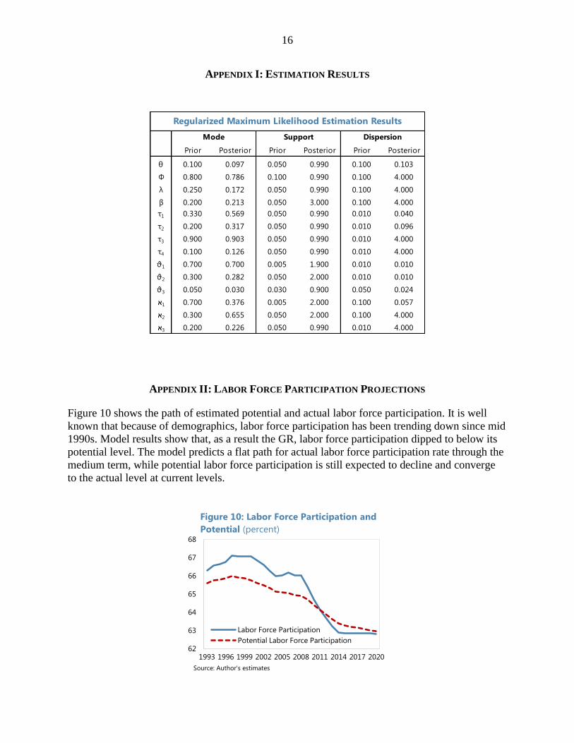
APPENDIX I: ESTIMATION RESULTS

APPENDIX II: LABOR FORCE PARTICIPATION PROJECTIONS

Figure 10 shows the path of estimated potential and actual labor force participation. It is well

known that because of demographics, labor force participation has been trending down since mid

1990s. Model results show that, as a result the GR, labor force participation dipped to below its

potential level. The model predicts a flat path for actual labor force participation rate through the

medium term, while potential labor force participation is still expected to decline and converge

to the actual level at current levels.

Prior Posterior Prior Posterior Prior Posterior

θ 0.100 0.097 0.050 0.990 0.100 0.103

Φ 0.800 0.786 0.100 0.990 0.100 4.000

λ 0.250 0.172 0.050 0.990 0.100 4.000

β 0.200 0.213 0.050 3.000 0.100 4.000

τ1 0.330 0.569 0.050 0.990 0.010 0.040

τ2 0.200 0.317 0.050 0.990 0.010 0.096

τ3 0.900 0.903 0.050 0.990 0.010 4.000

τ4 0.100 0.126 0.050 0.990 0.010 4.000

ϑ1 0.700 0.700 0.005 1.900 0.010 0.010

ϑ2 0.300 0.282 0.050 2.000 0.010 0.010

ϑ3 0.050 0.030 0.030 0.900 0.050 0.024

1א 0.700 0.376 0.005 2.000 0.100 0.057

2א 0.300 0.655 0.050 2.000 0.100 4.000

3א 0.200 0.226 0.050 0.990 0.010 4.000

Mode Support Dispersion

Regularized Maximum Likelihood Estimation Results

62

63

64

65

66

67

68

1993 1996 1999 2002 2005 2008 2011 2014 2017 2020

Labor Force Participation

Potential Labor Force Participation

Figure 10: Labor Force Participation and

Potential (percent)

Source: Author's estimates