Estimating Intertemporal Elasticity of Substitution: …/media/richmondfedorg/publications/... · ESTIMATING INTERTEMPORAL ELASTICITY OF SUBSTITUTION: THE CASE OF LOG-LINEAR RESTRICTIONS

ESTIMATING INTERTEMPORAL ELASTICITY

OF SUBSTITUTION: THE CASE OF

LOG-LINEAR RESTRICTIONS

C/&g-Sheng Mao *

1. Introduction

The modern theory of consumer behavior is con- cerned with how consumption adjusts to changing prices over time. When time is not involved, the de- mand for a normal consumer good declines as its relative price rises. Similarly, consumption at different points in time can be regarded as different goods, in which case the price that determines consumer behavior is the cost of today’s consumption in terms of tomorrow’s, or, equivalently, the cost of borrowing against the future. This price is called the real interest rate. When the expected real interest rate rises, consumers will attempt to defer current consumption by saving. Economists refer to the substitution between consumption at different points in time in response to changes in the real interest rate as intertemporal substitution in consumption.

The mechanism of intertemporal substitution plays an important role in the theory of consumption and macroeconomics in general. For instance, it implies that consumers will smooth their consumption given the expected time profile of real interest rates and lifetime wealth. Thus, consumers respond to an increase in current income by raising both current and future consumption. This effect has been widely used in analyzing a number of important issues. These include the behavior of aggregate consumption over time, the volatility of stock prices, and the burden of government deficits and social security. Because the smoothing of consumption tends to propagate current shocks into the future, this mechanism also helps explain persistence of business cycles. Further- more, the willingness of consumers to substitute intertemporally is a key determinant of the effec- tiveness of many government policies. Consider the recent debate over the reduction of capital gains tax rates. Proponents of the tax cut argue that it would

* The author received helpful comments from Michael Dotsey, Marvin Goodfriend, Robert Hetzel, Thomas Humphrey, and Yash Mehra.

encourage saving by making current consumption more expensive relative to future consumption, i.e., by raising the after-tax real return to saving. In fact, however, the influence of the tax cut on saving and investment depends crucially on the response of consumption to the corresponding changes in the intertemporal terms of trade. Thus, to evaluate the empirical effect of the tax cut, or in fact any policy that is meant to promote saving and economic growth, one must know the intertemporal elasticity of substitution.

While many authors have attempted to use actual data to estimate the intertemporal elasticity of substitution, their results are widely different. For example, using time series data in the United States, Hall (1988) concluded that there is no strong evidence that the elasticity is positive. By contrast, other studies have suggested a much stronger ten- dency of intertemporal substitution. The estimate obtained by Hansen and Singleton (1982, 1983), for instance, lies between 0.5 and 2, while the estimate obtained by Eichenbaum, Hansen, and Singleton (1986) can be as high as 10 depending on the data set used. The estimation by Hansen and Singleton (1988) even produces a negative elasticity estimate. At the very least, this wide range of figures raises questions regarding the reliability of the elasticity estimates.

This paper explores the reliability of estimates of the intertemporal substitution effect using Monte Carlo simulation. A model economy is specified in which the modeler himself selects the intertemporal elasticity of substitution. Then, using conventional statistical techniques, data generated from model simulations are used to estimate the elasticity. Since the elasticity’s true value is known, one can check how closely the estimates conform to the value that was chosen in constructing the data. This technique allows one to evaluate the performance of the conventional strategies for estimating the intertemporal elasticity of substitution. Since many of the empirical

FEDERAL RESERVE BANK OF RICHMOND 3

studies on intertemporal substitution ignore the potential wage effect on consumption, this paper also examines the consequence of misspecification error for a simulated model in which changes in the real wage have effects on consumption behavior. It is shown that ignoring the wage effect can cause a substantial bias in the estimation of the elasticity of substitution in consumption.

The next section outlines the notion of intertemporal substitution using a simple two-period model. Section 3 introduces a formal maximization problem, derives its first-order condition and discusses the estimation method. Section 4 lays out a model economy which serves a laboratory to generate simulation data. Section 5 summarizes the estimation results and Section 6 discusses the misspecification bias.

2. Intertemporal Substitution: A Two-Period Model

To clarify the notion of intertemporal substitution, consider a simple two-period consumer’s problem. The consumer is assumed to be endowed with a fured income yr in the first period and yz in the second period. In period 1, there is a capital market where the consumer may borrow or lend at a competitive real interest rate rr. Let cl and c2 denote consumption in period 1 and period 2, respectively. Then the budget constraint, expressed in present-value form, is CI + cz/(l +rr) = yr + yz/(l +rr). That is, the present value of current and future consumption must exhaust but not exceed the present value of the consumer’s income stream. The consumer’s problem is to choose cl and c2 in order to maximize his utility, u(cr, cz), subject to the budget constraint. This is a standard textbook problem. The consumer will ad- just his borrowing or lending so as to equate the marginal rate of substitution of cl for c2 with one plus the real interest rate. l In equilibrium, the consumer may be a net borrower or lender depending on his initial endowment position.

Figure 1 depicts the consumer’s equilibrium in which the horizontal and vertical axes measure cl and cz, respectively. In equilibrium, the consumer will choose to consume at point E at which the indifference curve is tangent to the budget line, which has slope -(1 +ri). As depicted, this consumer is a net lender and saving is equal to (yr -cl). Now, suppose the real interest rate rises from rr to rr ‘, so that the budget line rotates clockwise around the endowment

r In mathematical notation, this condition can be expressed as ur/ua = (1 +rr), where ui (i = 1, 2) is the marginal utility of consumption in period i.

Figure 1

point (yr, ~2) and has a steeper slope. A key question is how the consumption ratio cz/ci will respond to such a change. First, because consumption becomes relatively more expensive in period 1, there is a substitution effect that induces the consumer to substitute cz for cl by making more loans in the bond market. Because the consumer is lending, however, there is also an income effect that tends to raise consumption in both periods. Whether or not the consumption ratio cz/cr will rise depends upon the relative magnitude of these effects. For the purpose of this paper, the standard assumption seems reasonable, namely, that on balance cz/cr increases or that the income effect on cl is not strong enough to outweigh the substitution effect and the income effect on 122.2 As a result, the new equilibrium will be reached at point E ’ where the consumption ratio cz/ci is higher. Because of the assumption of constant elasticity, the increase in cz/cr is proportional to the increase in the real interest rate. The ratio of the percentage change in the rate of growth of consumption to the percentage change in the real

2 To be precise, the consumer’s utility function is taken to be homothetic and constant elastic. This assumption implies that the consumption good in each period is normal and that the slope of the indifference curve is constant along a given ray from the origin. Note that a utility function is called homothetic if the marginal rate of substitution depends only on the consumption ratio, and it is called constant elastic if the marginal rate of substitution is proportional to the consumption ratio. An explicit utility function will be specified in the next section.

4 ECONOMIC REVIEW, NOVEMBER/DECEMBER 1989

interest rate is called the intertemporal elasticity of substitution.

It is clear that the curvature (or the elasticity) of the indifference curve will determine the extent to which the consumer responds to changes in the real interest rate. The more elastic or less curved is the indifference curve, the greater the response will be. Figure 2 depicts the difference in the intertemporal substitution effect of two utility functions with different curvatures. For simplicity, assume that the initial equilibrium is the same so that both indifference curves UI and uz are tangent at the same point E to the budget line. Note that the curve ur has flatter curvature and is therefore more elastic. Suppose the real interest rate rises from rr to rr ‘. Then the new equilibrium will move from point E to point F in the case of ur, and to point G in the case of u2. Com- paring the consumption ratio CZ/CI at point F and G reveals that consumption grows faster when the indifference curve is more elastic. Thus, there is a positive relationship between the intertemporal elasticity of substitution and the elasticity of the indifference curve.

Now, suppose an econometrician who observes data on consumption and real interest rates over time wishes to estimate the intertemporal elasticity of

substitution. How would he go about doing this? The preceding analysis suggests that a natural approach is to think of each observation in time as represented

Figure 2

by the tangent point between the indifference curve and the budget line. As one traces out these equilibrium points over time, one essentially looks at the change in these tangent points which are determined by the curvature of the indifference curve. Thus, to estimate the elasticity one could simply regress the rate of growth of consumption on the real interest rate. This approach has been widely used by many authors to study the dynamic behavior of consumption [e.g., Hansen and Singleton (1983) and Hall (1988)].

The foregoing discussion illustrates how equilibrium conditions can be used to interpret economic data. Its implementation, however, requires more rigorous elaboration. For example, because of the stochastic nature of the data one must consider individual behavior under uncertainty. Also, in order to account for the evolution of consumption over time a fully dynamic model needs to be developed. Ac- cordingly, the next section presents a formal maximization problem in which the equilibrium conditions are explicitly used to construct the regression equation to be estimated.

3. The Optimization Framework

To start with, the consumer is assumed to have a time-separable utility function of the following form:3

I 1 [Ctl-l’o-l], if (T > 0 and

Uh) = 1 -l/a Of1

I Ma), ifa= 1

This utility function, which has been widely used in the literature, has the property that the elasticity of substitution in consumption4 is constant and is equal

3 A utility function is called time-separable when the marginal utility of consumption in a given period is independent of the level of consumption in other periods. This assumption simplifies the analysis.

4 The elasticity of substitution in consumption is defined as the partial derivative of the rate of change in consumption with respect to the marginal rate of substitution holding the level of utility fixed. In notation, this can be expressed as:

a Met + h)

Ci In[u’(ct)/u’(ct+ r)] u =; ’ I

where u ‘(.) denotes the marginal utility of consumption and ; a constant utility level. Note that this quantity measures an income-compensated substitution of consumption along a given indifference curve which is different from the uncompensated notion of intertemooral substitution. The two notions. however, turn out to be equivalent for two reasons. (1) The income effect is proportional to changes in wealth due to the homo- theticity of the utility function. (2) The real interest rate will pin down the marginal rate of substitution in equilibrium.


to the parameter (T. As will be seen shortly, this parameter will control the interest rate effect on consumption.

Now, let us consider the budget constraint. At the beginning of time t, the consumer carries kt units of capital from the last period. The capital is traded in a competitive market and yields a stochzs~ic rate of return rt in units of consumption goods. At the end of period t, the consumer collects interest income rtkt and principal kt. This sum is the only income that the consumer allocates between consumption ct and new capital kt + 1 to be carried into the next period. Thus, the consumer’s budget constraint for period t is ct + kt + 1 = (1 +rt)kt.

The consumer’s problem is to choose a path of consumption and capital, contingent on the realization of capital returns, that satisfies the budget constraint each period and maximizes the expected present value of lifetime utility over an infinite horizon.5 That is, given the initial capital stock ko, the consumer solves

max Eo[ F @u(ct)] t=O

subject to ct + kt + 1 = (1 +rt)kt for all t

where /3 is the time preference discount factor that lies between 0 and 1, and Eo is the expectation operator conditional on information at time 0.

The first-order condition (or Euler equation) of this problem is

u’(ct) = P Eb’(ct+l) (l+rt+dl It1 (1)

where It denotes the information set at time t.6 This equation is precisely a stochastic version of the equilibrium condition that the budget line must be tangent to the indifference curve as depicted in Figure 1.7 This equilibrium condition states that the marginal cost of investing an extra unit of consumption good at time t (i.e., the foregone marginal utility of consumption) should equal the marginal benefit from investing - this return being com-

5 The assumption that the consumer lives forever is here employed for analytical convenience only. The specification of a finite horizon problem will not alter the results of this paper.

6 The information structure is unspecified here. Note, however, that its specification is necessary for computing the conditional expectation.

’ Ignoring the expectation operator, equation (1) simply says that the ratio of the marginal utilities (expressed in units at time t) is equal to one plus ;he real interest r&e, which is the first-order condition for the two-period model in Section 2.

posed of the expected present value of the marginal utility of consumption times the investment proceeds at time t + 1 (principal plus interest). This condition implies that a small deviation from the optimal consumption plan will leave lifetime utility unchanged.

From an empirical standpoint, the above first-order condition is all that is needed to estimate the intertemporal elasticity of substitution. Obtaining the estimate involves use of a simple procedure to derive a regression equation from (1). First, given the constant-elastic utility function specified at the beginning of this section, (1) takes the form

EN (ct + l/cd - 1’0 (1 +rt+l) -l(It] = 0. (2)

This equation says that the residual (i.e., the term defined in the bracket) has a zero mean conditional on information available at time t. It implies that any variable included in the information set should be uncorrelated with the residual. These restrictions, referred to as orthogonality conditions, admit a class of instrumental variables procedures for estimating the parameters p and n [e.g., Hansen (1982) and Hansen and Singleton (1982)]. As can be seen, equation (2) is highly nonlinear and difficult to work with. A common procedure is to make distributional assumptions on certain variables at hand, and to transform the equation into a linear representation. This transformation renders the equation easy to estimate but its tractability is obtained at the cost of an extra assumption which may not be true.8

Specifically, assume that the measured growth of consumption ct + l/c* as well as the real interest rate (1 +rt + 1) has a lognormal distribution.9 This assumption implies that ln(xt+ I), where xt + 1 = P(ct + lh) - l’? 1 + rt + I), has a normal distribution with a constant variance v and a mean pt conditional on It. Using the lognormality assumption, we have E[xt + 1 [It] = exp[pt + v/Z]. Comparing with equation (2) yields exp[pt + v/2] = 1, which in turn implies pt = -v/2. Since, by definition, pt = E[ln xt + II&], it follows that

-v/2 = pt = In fi - l/a E[ln(ct+ I/ct)lIt]

+ EM1 +rt+ djL1.

* It should be noted, however, that distributional-independent methods such as the generalized method of moments proposed by Hansen (1982) is available for dealing with nonlinear prob- lems. The results pertaining to this procedure are beyond the scope of this paper, and are presented in Mao (1989).

9 A random variable X is lognormally distributed if the natural logarithm of X has a normal distribution. By definition, XY is lognormally distributed if both X and Y are lognormally distributed. If In(X) has a normal distribution with mean p and variance Y, then the mean of X is exp[p+v/Z].

6 ECONOMIC REVIEW. NOVEMBER/DECEMBER 1989

Multiplying both sides by 0 and arranging terms yields

EMct+dct)IItl = PO + u E[ln(l +rt+l)lItl,

where /30 = a[ln P + v/21. Let Et + 1 = ln(ct + l/et)

- Ellnkt + ht) lItI, then

Jn(ct+lW = PO + ~Elln(l+r~+d~Ll + et+l. (3)

Note that the expectational error Et + 1 is uncorrelated with the variables included in the information set, and is normally distributed with a zero mean and a constant variance. As can be seen, the parameter u identifies exactly the intertemporal elasticity of substitution. This equation is used later to estimate the parameter u.

Equation (3) implies that the mean of the rate of growth of consumption is shifted only by the condo- tionai mean of the real interest rate. That is, information at time t is helpful in predicting the rate of growth of consumption only to the extent that it predicts the real interest rate. Since the expectedreal interest rate is determined endogenously within the model, an instrumental variables procedure will be used to estimate the parameter u. This procedure amounts to two-stage least squares in which the first stage estimates the expected real rate using variables (instruments) contained in the information set con- sisting of observations on past consumption growth and real interest rates. The projected real interest rates are then used in equation (3) to estimate u. This procedure yields, a consistent estimate of the intertemporal elasticity of substitution.

As mentioned before, it has been difficult to pin down the parameter u. The point estimates vary widely, ranging from near 0 to 10. These results sug- gest that the linear regression equation (3) may not be a proper model for estimating the intertemporal elasticity of substitution. To examine this issue more closely, consider the following question. Given that the the true value of u is known, how accurately can that value be recovered by using (3) and the econometric procedure outlined above? A Monte Carlo experiment is carried out to answer this question.

4. The Data Generating Process

The first step of the Monte Carlo experiment is to write down a model economy whose output will be used to simulate the data. In particular, the economy is represented by a general equilibrium model in which the underlying production process

is explicitly specified. 10 This approach allows quan- tities as well as prices to be endogenously determined within the model.

The economy is similar to that described in Sec- tion 3 with the exception that the consumer now also plays the role of producer. In each period, the consumer carries from the previous period kt units of capital which are used to produce output. Due to the weather and other uncontrollable random factors, however, the volume of output is uncertain. To cap- ture such uncertainty, the technology is represented by a production function of the form: yt = AIF = XtktU, 0 < a < 1, where yt is output produced at time t and Xt is a random shock with a known probability distribution. The output may be con- sumed or invested. If invested, the capital will depreciate at a constant rate 6 (0 < 6 < 1) so that the investment at time t is defined to be it = kt + 1 - (1 - 6)kt. The agent is assumed to have a constant- elastic utility function as specified above. His problem is to choose a contingent plan for consumption and investment so as to maximize his expected lifetime utility. That is, the agent solves

max Eo[ c” @u(ct)l t=O

subject to ct + it = XtF(kt) for all t.

The solution of the above maximization problem consists of a sequence of consumption and investment outcomes over time, contingent on the realization of the random shock Xt. In this way the model generates the consumption data for estimating the intertemporal elasticity of substitution u in (3) above. The model also generates an implied real interest rate time series, needed to estimate (3). To see this, consider the first-order condition:

u’(ct) = P &(u ‘(ct + I) IA, + IF ‘(k + 1)

+ (1 - ml. (4)

The intuition behind (4) goes as follows. Suppose at time t the agent decides to carry one extra unit of consumption good to the next period, which will cost him, in utility terms, the marginal utility of consumption. The gain that results is the expected present value of the marginal utility of consumption times the extra output that can be produced at time t + 1, which is equal to the sum of the marginal product

lo Readers familiar with the literature on economic growth will recognize that the model specified is a standard optimal growth model as studied by Brock and Mirman (1972).


of capital and the amount of capital that is left over after depreciation. Equating the cost and benefit in equilibrium yields equation (4). As can be seen, equation (4) is identical to the first-order condition of the consumer’s problem [equation (l)] except that the real interest rate is replaced by the rate of return on investment, i.e., the marginal product of capital minus the depreciation rate.

Because the optimization problem does not have a closed-form solution, a numerical method will be used to solve the problem. Specifically, a dynamic programming algorithm is employed to approximate the solution over a discrete state space.” It is assumed that the production shock Xt can take 5 distinct values over the set [0.9, 1.11, i.e., 0.9, 0.95, 1 .O, 1.05, 1.1, and that it evolves over time accord- ing to the following Markov transition probability: l*

r

! 0.50 0.25 0 0 0 0.30 0.50 0.25 0 0 0.20 0.25 0.50 0.25 0.20 0.25 0.50 0.30 0 0 0.25 0.50 0 0 0

This transition matrix implies that the random shock will be, to some degree, persistent over time because the probability of staying in the same state is higher than that of switching to other states. The choice of this transition matrix is motivated in part by the fact that the actual production shocks in the United States, as measured by the Solow residual,13 are positively correlated over time. The estimation results reported below do not appear to be sensitive to the specification of this transition matrix. Other parameters that are held constant throughout the experiment are: 0 = 0.96, (Y = l/3 and 6 = 0.1. These numbers are also chosen to reflect data ac- tually generated from the United States economy. For example, the value of /3 implies a real interest rate of about 3 percent a year, which is close to what is observed in the United States. The (Y value is

*I The algcrithm, known as the value successive approximation, iterates on the problem’s value function over a discrete state space. Technical details can be found in Bertsekas (1976).

r* The elements of this transition matrix assign the probability of moving from one state to another. For example, if the value of the production shock at time t is 1.0 (the third row), then there is 25 percent chance that it will move to 0.95 or to 1.05 in the next period and 50 percent chance that it will stay in the same state.

I3 Whether the Solow residuals, i.e., the residuals arising from the regression of a production function, truly represent the underlying shocks of the economy is a controversial matter. This issue is ignored here.

chosen to reflect the output elasticity of capital in the United States-that elasticity figure being roughly one-third and holding fairly steady over a long period of time. Given these parameters’ values, the model is solved for a set of four different values for u (0.1, 0.25, 1.0, and 2.5).

Since no interest attaches to the numerical solution per se, it is not reported. It is crucial, never- theless, to have some idea about the accuracy of the approximation procedure before the solution can be used to generate random samples. This accuracy can be assessed by checking whether the data generated from the model satisfy the first-order condition, i.e., equation (2). Let ht + r = fl(ct + i/et) - “O( 1 +rt + 1) - 1, then (2) can be rewritten as E[ht + rl~t] = 0. As mentioned before, this condition implies a set of orthogonality conditions which require that the residual ht + r be uncorrelated with any variable included in the information set. Let zt be a subset of It; then these conditions imply that the first sample moment of the cross product ht + rzt should be close to zero for a sufficiently large sample. The vector zt consists of a constant of ones plus the past observations on consumption growth ct + i/et and the real interest rate (1 + rt + 1). The constant term is included because the unconditional mean of ht + i must be zero. Reported in Table I are, for each u value, the sample means of the product ht+ rzt based on a realization of 2000 observations. The number of lags used for consumption growth and the real interest rate is 2, so in total there are 5 variables in the vector zt. The same set of variables will be used as instruments in the econometric procedure of the next section. As can be seen, the means are very small and insignificantly different from zero (standard deviations of the mean are reported in parentheses). This result also holds for smaller sample sizes which are not reported here. To conclude, the data generated from the solution procedure fulfill the Euler equation and have negligible approximation error.

5. Estimation Results

This section pursues the second step of the Monte Carlo experiment. The intertemporal elasticity of substitution u is estimated using equation (3) and data generated from the simulated economy discussed in Section 4. The objective here is to see if this strategy produces a reliable estimate of u.

A brief description of the simulation procedure follows. First, for each of the four u values considered in the experiment are generated a number of random samples from the artificial economy. These observations are then employed to estimate the parameter u. This process produces a sampling distribution of


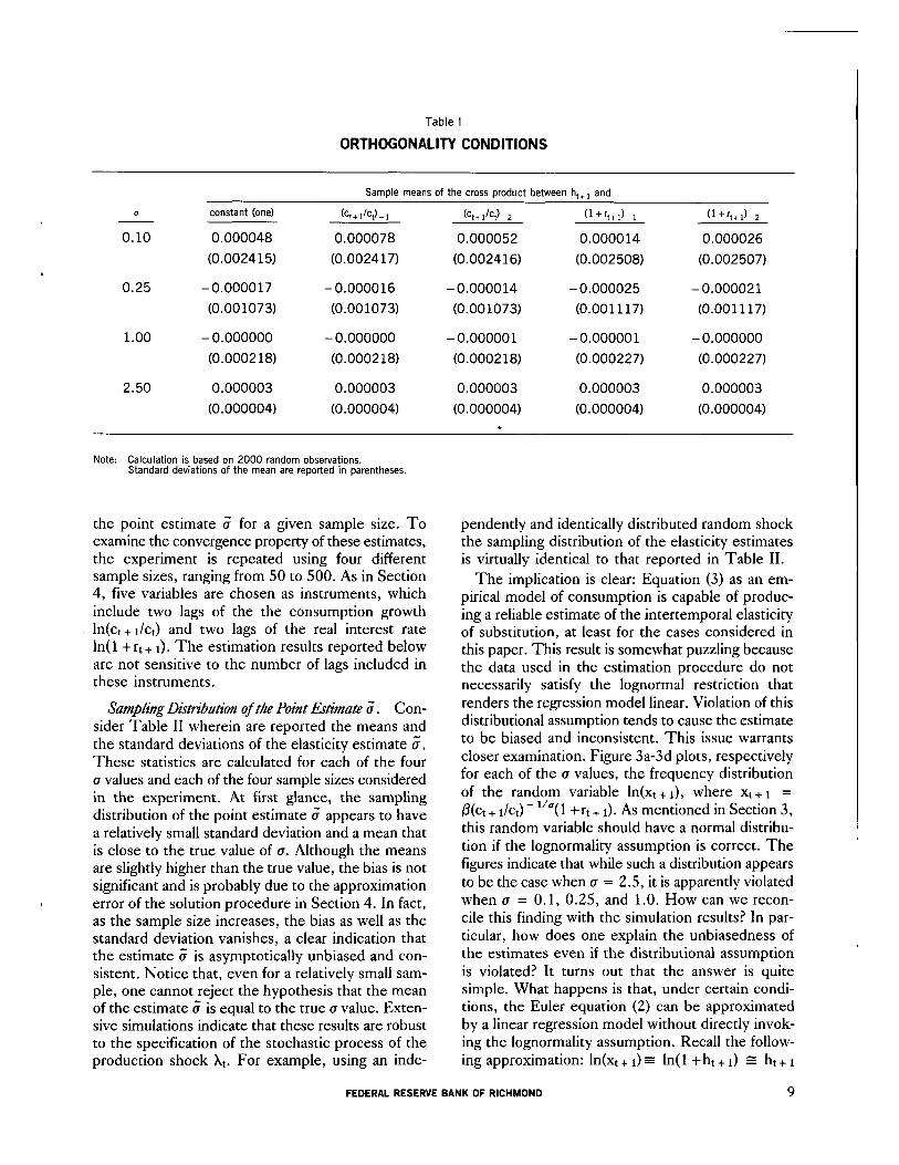
Table I

ORTHOGONALITY CONDITIONS

Sample means of the cross product between h,,, and

cl

0.10

0.25

constant (one)

0.000048

(0.002415)

-0.000017

(0.001073)

1.00 - 0.000000 - 0.000000 -0.000001 - 0.000001 - 0.000000

(0.000218) (0.000218) (0.000218) (0.000227) (0.000227)

2.50 0.000003 0.000003

(0.000004) (0.000004)

(ct + Jet) - 1 (ct+1’ct)-2 (l+r,+J-, (l+r,+,)-,

0.000078 0.000052 0.000014 0.000026

(0.002417) (0.002416) (0.002508) (0.002507)

-0.000016

(0.001073)

-0.000014

(0.001073)

-0.000025

(0.001117)

-0.000021

(0.001117)

0.000003

(0.000004) .

0.000003

(0.000004)

0.000003

(0.000004)

Note: Calculation is based on 2000 random observations. Standard deviations of the mean are reported in parentheses.

the point estimate a’ for a given sample size. To examine the convergence property of these estimates, the experiment is repeated using four different sample sizes, ranging from 50 to 500. As in Section 4, five variables are chosen as instruments, which include two lags of the the consumption growth ln(ct + r/c*) and two lags of the real interest rate ln( 1 + rt + 1). The estimation results reported below are not sensitive to the number of lags included in these instruments.

Sampling Di.mhtion of the Point Estinzate a”. Con- sider Table II wherein are reported the means and the standard deviations of the elasticity estimate a, These statistics are calculated for each of the four u values and each of the four sample sizes considered in the experiment. At first glance, the sampling distribution of the point estimate a” appears to have a relatively small standard deviation and a mean that is close to the true value of cr. Although the means are slightly higher than the true value, the bias is not significant and is probably due to the approximation error of the solution procedure in Section 4. In fact, as the sample size increases, the bias as well as the standard deviation vanishes, a clear indication that the estimate 6 is asymptotically unbiased and consistent. Notice that, even for a relatively small sample, one cannot reject the hypothesis that the mean of the estimate a’ is equal to the true (T value. Exten- sive simulations indicate that these results are robust to the specification of the stochastic process of the production shock Xt. For example, using an inde-

pendently and identically distributed random shock the sampling distribution of the elasticity estimates is virtually identical to that reported in Table II.

The implication is clear: Equation (3) as an empirical model of consumption is capable of produc- ing a reliable estimate of the intertemporal elasticity of substitution, at least for the cases considered in this paper. This result is somewhat puzzling because the data used in the estimation procedure do not necessarily satisfy the lognormal restriction that renders the regression model linear. Violation of this distributional assumption tends to cause the estimate to be biased and inconsistent. This issue warrants closer examination. Figure 3a-3d plots, respectively for each of the u values, the frequency distribution of the random variable ln(xt+ I), where xt+ 1 =

Pht + lh) - 7 1 + rt + 1). As mentioned in Section 3, this random variable should have a normal distribution if the lognormality assumption is correct. The figures indicate that while such a distribution appears to be the case when (T = 2.5, it is apparently violated when u = 0.1, 0.25, and 1.0. How can we recon- cile this finding with the simulation results? In particular, how does one explain the unbiasedness of the estimates even if the distributional assumption is violated? It turns out that the answer is quite simple. What happens is that, under certain conditions, the Euler equation (2) can be approximated by a linear regression model without directly invok- ing the lognormality assumption. Recall the following approximation: ln(xt + 1) = ln( 1 + ht + 1) E ht + 1


True (I

0.10

0.25

1.00

2.50

Table II

SAMPLING DISTRIBUTION OF THE POINT ESTIMATE 6 (a)

Number of Number of observations simulations

50 780

150 520

300 480

500 400

50 780

150 520

300 480

500 400

50 780

150 520

300 480

500 400

50 780

150 520

300 480

500 400

(I

Mean s.d.

0.257039 0.155508

0.172956 0.070608

0.142281 0.048254

0.129667 0.038071

0.414662 0.205668

0.321207 0.100773

0.286916 0.070803

0.273533 0.056699

1.126016 0.275207

1.044132 0.150668

1.017989 0.105218

1.009004 0.084706

2.504959 0.021614

2.503065 0.011713

2.502775 0.007199

2.502399 0.005670

ta) These results are based on assumed highly persistent shocks specified in the text. Experiments with independently and identically distributed (iid) shocks yield similar results.

for xt + 1 close to one or ht + 1 close to zero. Since the condition that ht + 1 be close to zero is approxi- mately true for our data (see Table I and Figure 3), the linear regression equation (3) can be viewed as an approximation to the Euler equation (2). It is worth mentioning that in the United States the rate of growth of consumption is about 2 percent a year and the annual real rate of interest is about 3 percent, suggesting that xt + 1 is close to one.

Hypothsk Testing Based on the regression model, a number of hypotheses can be tested. This subsec- tion focuses on the simple hypothesis that the parameter u is equal to its true value. As usual, this hypothesis can be tested using a conventional t statistic. Since we know the true u value that is used to generate the data, we are interested in the Type I error for testing this hypothesis, that is, the proportion of time that the null hypothesis is rejected when it should have been accepted. The test results are summarized in Table III. As can be seen, the rejection frequency of the true model is higher than expected. This is particularly clear when ~7 is small.

For example, at a 5 percent significance level, about 20 percent of the time one will reject u = 0.1 even though the sample size is relatively large (say, 500). At a 10 percent significance level, the proportion rises to above 30 percent. Although the rejection frequencies are somewhat moderate for other cases, it seems reasonable to conclude that the risk of committing the Type I error is still too high. Again, this result may appear puzzling because the point estimate is fairly close to the true parameter value. A moment’s reflection reveals that these errors stem from the standard error of the estimate’s being so small that the true parameter value lies outside of the confidence region.

6. Misspecification Bias with Variable Labor Supply

Many of the empirical studies on intertemporal substitution abstract from the interaction between consumption and labor supply decisions and thereby ignore the potential effect on consumption of changes in the wage rate [for example, Hansen and Singleton (1983) and Hall (1988)]. As noted before, such a simplification implies that the growth of consumption is determined only by the expected real interest rate. This section examines a more realistic model in which an individual chooses both consumption and labor supply at the same time. Such a model implies that changes in the real wage can have important effects on consumption behavior. It will be shown that failure to incorporate these effects can result in a sizable bias in estimating the intertemporal elasticity of substitution.

As in the previous case, the starting point is a simple two-period model. For comparison, refer to Figure 1 in which the equilibrium moves from point E to E’ when the real interest rate rises. What would


Figure 3

FREQUENCY DISTRIBUTION OF THE TRUE RESIDUALS

(a): u = 0.10

141

10 1

E8 8 b,

-0.2 -0.1 0.0 0.1 0.2 -0.016 -0.008 0.000 O.dO8 0.016

(b): u = 0.25

71

6

-0.06 -0.02 0.02 0.06 0.10 - 0.0004 - 0.0002 0.0000 0.0002 0.0004

happen if the consumer is allowed to supply work effort in the labor market and earn wage income? In general, the point E ’ will no longer be an equilibrium because the labor supply decision, even if the wage rate remains unchanged, is likely to alter the rate of substitution in consumption. In this case, the equilibrium point can go in either direction depending upon the extent to which labor supply affects the marginal utility of consumption. In order to make a specific prediction, one needs an explicit model.

The model considered below is similar to that described in Section 3. First, the consumer’s utility function is assumed to depend on consumption ct and leisure time It and has the following form:

8

F t! 6 2

(d): u = 2.50

6c

5’

UWt) =

&$C’@ lt(l -~I~-:‘“,,~~~, z 1

f3 In ct + (l-0) In It, ifa = 1

This utility function is similar to that specified before and is constant elastic with respect to a “composite good” defined as a Cobb-Douglas function of consumption and leisure. The parameter 8 lies between 0 and 1. As will be seen shortly, the parameter u can still be identified as the intertemporal elasticity of substitution. But, more importantly, the u parameter controls the effect of leisure on the marginal utility of consumption. Specifically, when


Table III

REJECTION FREQUENCY OF THE

NULL HYPOTHESIS: u = true da) (Type I Error)

0.25 50 23% 35%

150 16% 24%

300 12% 19%

500 11% 20%

1.00 50

150

300

500

2.50 50

150

300

500

True 0

0.10

Number of observations

50

150

300

500

Significance level

5 Percent 10 Percent

26% 39%

21% 32%

18% 29%

19% 33%

19%

13%

7%

9%

11%

9%

10%

12%

29%

19%

14%

14%

19%

19%

20%

20%

(a) These results are based on assumed highly persistent shocks specified in the text. Experiments with iid shocks yield much higher rejection frequencies (more than 50 percent).

(I > 1, consumption and leisure are gross comple- ments because an increase in leisure will raise the marginal utility of consumption.14 The opposite is true when u < 1. The value of u will dictate the effect of the real wage on consumption.

It is important to note that the wage effect on consumption will depend on the form of the utility function. In particular, if the utility function is additively separable,15 then the marginal utility of consumption will be independent of the choice of leisure. In this case, changes in the real wage have no effect on consumption. Consequently, equation (3) will still be the correct specification for consumption. This assumption has been maintained by most authors [e.g., Hall

r4 That is, uCr > 0 if u > 1, where uCr is the partial derivative of the marginal utility of consumption with respect to leisure time.

I5 A utility function u(x,y) is additively separable if it has the form: m(x) + n(y). This class of utility functions is not limited to the logarithmic case specified in the text.

(19SS)l. Since there is no direct evidence on whether the utility function is separable, it is useful to check how serious the misspecification bias could be.

To proceed, suppose the consumer solves the following maximization problem:

max I%] c” P’u(ctJ41

L

t=O .:

s.t. ct + kt + r = (1 +rJkt + wtnt for all t

where wt is the wage in terms of consumption goods and nt = 1 - It is work effort. Following the same derivation procedure as in Section 3 and assuming lognormality, it can be shown that consumption now obeys the following equation:

ln(ct+dct) = PO + u EM1 +rt+ d\Itl + ,&EMwt + dw)~Itl + Et + I (5)

where fir = (1 - t9)(1 - a). Except for the addi- tional term that captures the effect of wage growth on consumption, this equation is similar to equation (3) which abstracts from the labor supply decision. As can be seen, the parameter u still measures the interest rate effect on consumption. However, the wage will have a positive effect (pr > 0) on consumption growth if u < 1, and negative effect (/3r < 0) if u > 1. This is so because u < 1 implies ucr < 0, so that when the real wage rate rises, leisure will decline and the marginal utility of consumption will rise. As a result, consumption must rise to restore the equilibrium. Note that when u = 1, a change in the real wage has no effect on consumption because the utility function is additively separable in this case.

What would happen if the true data were generated from the above model, and yet the econometrician erroneously ignored the wage effect and instead used (3) to estimate a? This is a typical specification error in which an important variable is omitted from the regression. Apparently, the estimate for u will be biased, with the magnitude of the bias measured by the true value of /I1 times the auxiliary regression coefficient of the wage growth on the real interest rate.r6 Thus, if the real interest rate and the growth of real wages are positively (negatively) correlated, then ignoring the wage effect leads to a downward (upward) bias if u > 1, and an upward (downward) bias if u < 1. Notice that, if the real interest rate and the growth of real wages are un-

I6 This is a standard result on specification bias. See Maddala (1977).


correlated, then the elasticity estimate using (3) will be unbiased.

One way to evaluate the extent of the above misspecification bias is to conduct a Monte Carlo simulation. As in Section 4, the data are generated from a model economy in which the production function is assumed to be yt = Xtkt%t(’ - a), 0 < CY < 1.” The production shock is generated in the same way

d as before. Other parameters fixed in the experiment are fl = 0.96, 6 = 0.1, cx = l/3, and 0 = 0.3. Following the same procedure, u is estimated using (3) as well as (5). Because of the difference in the specification, the instruments used in estimating equation (5) include lags of ln(ct + I/et), ln( 1 +rt + 1) and ln(wt + l/wt). These instruments are used to project the expected real interest rate as well as expected wage growth. Table IV summarizes the means and the standard deviations of the estimated bias. It is clear that when the model is correctly specified, i.e., equation (S), the estimated bias is small and in- significant. However, the bias associated with equa- cion (3) is sizable. In particular, when (T = 0.25, the

I7 Specifically, the data are generated from a real business cycle model:

max &[ c” /3’u(ct, 1 -nt)] t=O

s.t. ct + kt+l = XtFhnt) + (1 - 6)kt

where F(. , .) is the production function which depends on capital and labor. As in Section 4, the equilibrium prices can be com- puted directly from the solution of the optimization problem. In particular, the real interest rate is the marginal product of capital minus the depreciation rate while the real wage is just the marginal product of labor.

point estimates are scattered around the value of 2, and when u = 2.5, the point estimates are less than one and in some cases close to zero. These results show that ignoring a potential wage effect on consumption can introduce a substantial bias in the estimation of the elasticity of substitution.

7. Concluding Remarks

The results of this paper can be summarized suc- cinctly. First, for a moderate sample size (perhaps in the range of 100 to 150), the point estimate of the intertemporal elasticity of substitution produced by the linear model tends to be unbiased with small standard errors. This result implies that the loglinear model, despite its simplicity, is a useful and convenient framework for estimating the intertemporal elasticity of substitution. Second, the conventional t test tends to over-reject the true model. Therefore, one must be careful in drawing conclu- sions from this test. Third, if the estimated equation is erroneously specified and omits the effect of the real wage on consumption, then the bias of the elasticity estimate is sizable. One should not conclude, however, that it is always necessary to use the extended model to estimate the elasticity; similar

biases could arise in the extended model if it is also misspmified.

In general, any econometric method founded on an intertemporal maximization problem and its resulting Euler equation is bound to be sensitive to measurement errors. Such errors are particularly characteristic of consumption data, especially data on durable goods consumption. They are perhaps

Table IV

MISSPECIFICATION BIAS

Bias: 0 - o

True o Number of Number of

observations simulations

0.25 50 600

150 400

300 400

500 300

2.50 50 600

150 400

300 400

500 300

Correct: Eq. (5) Incorrect: Eq. (3)

Mean sd. Mean s.d.

0.119739 0.066889 1.958582 0.667838

0.053412 0.049080 1.732927 0.453833

0.030032 0.033670 1.692648 0.326624

0.022194 0.027314 1.670278 0.267501

0.433372 0.522541 - 1.770626 0.310914

0.174026 0.330437 - 1.657668 0.189137

0.080718 0.220140 - 1.607193 0.129013

0.057523 0.184815 - 1.596351 0.108533


the most important reason why empirical studies have task. There is no easy solution to this identification not been able to pinpoint the intertemporal elas- problem. There are at present more sophisticated ticity of substitution. As shown above, however, even test procedures, such as tests of overidentifying if the data are properly measured, the econometri- restrictions, that may be used to discriminate among cian still must choose a correct specification. Iron- different models. However, the properties of such ically, the data themselves are supposed to aid in this test statistics under misspecification are not clear.

References

Bertsekas, Dimitri P. Dynamic Pmgramming and Stochastic Con- &. New York: Academic Press, 1976.

Brock, W. J., and L. J. Mirman. “Optimal Economic Growth and Uncertainty: The Discounted Case.” Jownaf of Lhomic Theory 4 (June 1972): 479-513.

Eichenbaum, Martin S., Lars Peter Hansen, and Kenneth J. Singleton. “A Time Series Analysis of Representative Agent Models of Consumption and Leisure Choice Under Uncer- tainty.” Working Paper No. 1981. National Bureau of Economic Research, July 1986.

Hansen, Lars Peter, and Kenneth J. Singleton. “Generalized Instrumental Variables Estimation of Nonlinear Rational Expectations Models.” Econotnetn~a 50 (September 1982): 1269-86.

. “Stochastic Consumption, Risk Aversion, and the Temporal Behavior of Asset Returns.“Jounalof Pofiri- cal Economy 91 (April 1983): 249-65.

. “Efficient Estimation of Linear Asset Pricing Models with Moving Average Errors.” Manuscript. Univer- sity of Chicago, April 1988.

Hall, Robert E. “Intertemporal Substitution in Consumption.” humaf of Po.kicd Economic 96 (Apd 1988): 339-57.

Hansen, Lars Peter. “Large Sample Properties of Generalized Method of Moments Estimators.” Economettica 50 (july 198.2): 1029-54.

Maddala, G. S. Economerris. New York: McGraw-Hill, 1977.

Mao, Ching-Sheng. “Euler Equation Estimation: A Simulation Study.” Manuscript, Federal Reserve Bank of Richmond, August 1989.


Documents

Estimating Intertemporal Elasticity of Substitution: …/media/richmondfedorg/publications/... · ESTIMATING INTERTEMPORAL ELASTICITY OF SUBSTITUTION: THE CASE OF LOG-LINEAR RESTRICTIONS