Elasticity of Substitution, Price Effect and Sustainable

Prague Economic Papers, 2021, 30 (2), 189–215, https://doi.org/10.18267/j.pep.764 189

EL ASTICIT Y OF SUBSTITUTION, PRICE EFFEC T AND SUSTAINABLE FERTILIZER USE: A TR ANSLOG AND SUR ANALYSIS IN CHINA *

Yipu1Pangab , Jingqi Dangac , Wei Xud

AbstractFertilizer has brought great pressure to sustainable ecological environment. Research on the effect of price on fertilizer use as well as the substitution relationship of fertilizer and other input factors of agricultural production is of great importance for green, efficient, and intensive agricultural production in the world. This study first constructs translog cost functions and models of elasticity, then uses the factor input and price data from 2004 to 2016 to measure the price elasticity of fertilizer demand, and the elasticity of factor substitution in China’s maize and cabbage production. The results suggest that: the price elasticity of fertilizer demand is in a low elasticity range; there is a compensation relationship between fertilizer and labour and a substitution relationship between fertilizer and machinery in China’s maize production, while these relationships in China’s cabbage production are opposite.

Keywords: Elasticity of substitution, price effect, sustainable fertilizer use, translog, SURJEL Classifications: Q10, Q58, D24, C51

1. Introduction

The history of the world’s agricultural development shows that fertilizer is the most efficient means of increasing production. Fertilizer is also an essential factor for modern agriculture (Dawson and Hilton, 2012). Fertilizer has contributed extremely to the development of China’s agricultural production, as well as national economy (Wang et al., 2008). Without fertilizer, China is not able to use only 7% of the world’s total arable land resources to feed 1.3 billion

* The authors acknowledge the financial support of the National Natural Science Foundation of China (Grant No. 71903031) and the Social Science Planning Project of Fujian Province (Grant No. FJ2018C020).

a China Academy for Rural Development, Zhejiang University, Hangzhou, Zhejiang, Chinab School of Public Affair, Zhejiang University, Hangzhou, Zhejiang, Chinac School of Management, Zhejiang University, Hangzhou, Zhejiang, Chinad School of Public Administration, Fujian Agricultural and Forestry University, Fujian, China Email: [email protected]

https://orcid.org/0000-0002-7668-9647

https://orcid.org/0000-0002-3830-5235

Prague Economic Papers, 2021, 30 (2), 189–215, https://doi.org/10.18267/j.pep.764190

Chinese people, which accounts for nearly a fifth of the world’s total population. The contin-uous growth of grain production from 2001 to 2016 in China was accompanied by a con-tinuous increase in fertilizer use, thereby showing a strong positive correlation (Figure 1).

However, fertilizer use in China has exceeded international standards in recent years. China’s fertilizer use was about 60 million tonnes in 2016, which is nearly half of Asia’s total fertilizer use (49.5%), accounts for 28.5% of the world’s total fertilizer use in the same year, and ranks first in the world. China’s average fertilizer application intensity reached 453.6 kg/ha, which is approximately 2.5 times than that in Asia and 3.8 times than that in the world (Table A.1). In addition, it is far beyond the upper limit of the international standard for safe fertilization (225 kg/ha), which has been set to prevent water pollution (Ju et al., 2016; Ma et al., 2019).

Figure 1: China’s grain output and fertilizer input from 2004 to 2016

Note: The figure describes the common growth trend between China’s grain production and fertilizer input.

Source: China Statistical Yearbook (National Bureau of Statistics of China, 2017).

Previous studies have shown that excessive fertilizer use and low utilization efficiency in China have led to serious agricultural non-point pollution and caused environmental degradation of agricultural soil, rivers, lakes, and the atmosphere (Wang et al., 2008; Ni and Zheng, 2012). Overuse of fertilizer also has a negative impact on the metabolism of organic compounds in plants, causing undue accumulation of nitrates and nitrites in plants. What’s more, fertilizer over-application makes nitrogen oxides enter the atmosphere, which can not only cause greenhouse effect but also damage the ozone layer (Wu, 2011; Takeshima and Nkonya, 2014).

65

60

55

50

45

40

35

30

700

650

600

550

500

450

400

350

300 2004 2005 2006 2007 2008 2009 2010 2011 2012 2013 2014 2015 2016

Grain yield Fertilier use


The environmental pollution originating from excessive fertilization has aroused the government’s great attention. The Chinese government has emphasized that China will strengthen the prevention of agricultural non-point pollution and further promote the reduction and efficient use of fertilizer. This series of policy proposals indicates that advocating the efficient application of fertilizers and promoting the green growth of agricultural production have become an important theme in China’s agricultural development (Xiong and Wu, 2017). Therefore, the exploration of influence factors of fertilizer use in China based on current policy guidance and research status is of great theoretical and practical significance.

Existing studies mainly focus on the impact of social factors and household characteristics on households’ fertilization behaviour, based on microdata from developing countries and regions. Some studies have analysed households’ determinants of fertilizer application (Abdoulaye and Sanders, 2015; Tian et al., 2015; Mustapha and Said, 2016), whereas others have analysed the cause of excessive fertilizer application (Takeshima and Nkonya, 2014). However, there is a research gap in that most studies lack analysis of the impact of factor price on fertilizer use, this study fills the gap by analysing the price elasticity of fertilizer demand and the elasticity of substitution between fertilizer and other agricultural input factors.

Based on a literature analysis and empirical facts, we constructed a translog cost function model and equations of shadow elasticity of substitution (SES). We use the models and the seemingly unrelated regression (SUR) to measure fertilizer price elasticity with the factor input and price data, the elasticity of substitution between fertilizer and labour, and the elasticity of substitution between fertilizer and machinery in China’s maize and cabbage production.

Our study contributes to previous research in three ways. Firstly, it provides a general representative rural household model for analysing the impact of price effect and substitution effect on households’ fertilization decision. This model offers a theoretical basis and analytical framework for empirical research and policy implications, and is not limited to the calculation of several economic indicators. Secondly, this study uses the SUR method, and long-term and multi-region panel data for empirical analysis of the price effect and substitution effect of two representative crops. This study makes up for the shortcomings of the existing literature, such as a single sample, imperfect data and inaccurate estimates, and enriches the existing empirical research results. Finally, the research findings provide guidance for China to formulate and adjust fertilizer policies, help governments and farmers in agricultural developing countries use fertilizers reasonably and efficiently to promote intensive agricultural production, and further promote prevention of global agricultural non-point source pollution and sustainable development of world agriculture.


2. Conceptual Framework

Microeconomic production theory shows that demand for production factors is influenced by the price of factors themselves and the price of other factors. The degree of response of factor demand to its price change is the price elasticity of demand, which is the ratio between the percentage of change in factor demand and the percentage of change in factor price (McFadden, 1963; Liu et al., 2014): if the demanded quantity of a factor exhibits a large change in response to changes in its price, it is termed elastic, if the demanded quantity of a factor show a small change in response to changes in its price, it is termed inelastic. Given the output level, the degree of response of factor demand to price changes in other input factors is the elasticity of substitution, which is the ratio between the percentage of change in factor demand and the percentage of change in price of other factors (Binswanger, 1974; Clark et al., 2013): if the price of factor A declines and producers are encouraged to increase the input of factor B, then there is a complementary relationship between factors A and B; if the opposite is true, there is a substitution relationship between factors A and B.

As an important factor in agricultural production, the demand for fertilizer is closely related to the price of fertilizer, labour and machinery faced by farmers in production decisions (Liu et al., 2014; Hu and Yang, 2015; Gao et al., 2018). Considering the following general representative household agricultural production decision-making model:

T = Pf (La, F, M) − NF − SM + WLn (1)

where T is household income, P is the agricultural product price, f(*) is the agricultural production function, La is the agricultural labour input, F is the fertilizer input, M is the agricultural machinery input, W is the labour price, N is the fertilizer price, S is the agricultural machinery price, and Ln is off-farm labour. Let L be the total labour force; then we have Ln = L − La − Lc, Lc means leisure. In order to simplify the analysis, we assume that L and Lc are fixed, and Equation 1 can be rewritten as follows:

T = Pf (La, F, M) − WLa − NF − SM + WL − WLc (2)

A household’s optimal fertilizer demand can be obtained by taking the first partial derivative of T:

F* = F (P, N, S, W) (3)

According to Equation 3, ∂F*/∂N is the price elasticity of fertilizer demand, and according to relevant microeconomic theories, ∂F*/∂N < 0.║∂F*/∂N║ > 1 means that fertilizer


demand is elastic;║∂F*/∂N║∈ (0, 1) means that fertilizer demand is inelastic. ∂F*/∂W and ∂F*/∂S respectively represent the elasticity of substitution between fertilizer and labour, and the elasticity of substitution between fertilizer and machinery. ∂F*/∂W > 0 indicates that there is a substitution relationship between fertilizer and labour, whereas if ∂F*/∂W < 0, there is a complementary relationship; ∂F*/∂S > 0 indicates that there is a substitution relationship between fertilizer and machinery, whereas if ∂F*/∂S < 0, there is a complementary relationship. However, the influence of price elasticity of demand and elasticity of substitution on fertilizer demand is relatively complex, and it is difficult to directly obtain the price elasticity of demand and elasticity of substitution through the conceptual framework:

(1) A change in fertilizer market price will lead to a reverse change in household fertilizer input, and the degree of this change depends on the price elasticity of fertilizer demand: if fertilizer demand is elastic, the amount of fertilizer input will largely depend on the market price of fertilizer; therefore, the government can intervene in farmers’ input of fertilizer using price policies such as adjusting fertilizer subsidies to realize rational and effective application of fertilizer. If fertilizer demand is inelastic, a change in fertilizer market price will not lead to a big change in household fertilizer input; thus, it is no longer effective to restrict farmers’ excessive fertilizer application via price policy.

(2) The relationship between fertilizer and labour will significantly affect the decision of farmers on fertilizer application, but the relationship is relatively complex: on the one hand, fertilizer is mainly applied manually in China, and the input of fertilizer needs the assistance of labour force; therefore, there may be a complementary relationship between the two factors, so a rising labour price will reduce the input of fertilizer by reducing labour demand in agricultural production; the government can adjust the amount of fertilizer used in agricultural production through agricultural technical training, encouraging migrant workers and other policies; on the other hand, the rising labour prices will lead farmers to neglect field management and increase the amount of fertilizer by “fewer fertilizer application times and more fertilizer application amounts” to ensure production; therefore, there is a substitution relationship between the two factors; the government needs to provide agricultural production subsidies, encourage agricultural diversification to appropriately reduce the price of labour to adjust the amount of fertilizer used in agricultural production.

(3) The relationship between fertilizer and machinery will significantly affect farmers’ decision on fertilizer application, but the relationship is also complex: on the one hand, in recent years, the integration of irrigation, fertilizer, pesticide and machinery in China’s agricultural production has developed rapidly, more and more crops have been fertilized using agricultural machinery, which may result in a complementary relationship between


the two factors: an increase in the price of machinery will reduce the amount of fertilizer input; the government can adjust the amount of fertilizer used in agricultural production by reducing subsidies for agricultural machinery, increasing agricultural technical training and promoting refined operations; on the other hand, the use of some agricultural machinery can effectively promote the dissolution and absorption efficiency of fertilizers in soil, which can keep the yield unchanged while reducing fertilizer application, so there is a substitution relationship between the two factors: the government can adjust the amount of chemical fertilizer used in agricultural production by increasing subsidies for agricultural machinery and advocating appropriately scaled operation of agriculture.

To sum up, the price elasticity of fertilizer demand and the elasticity of substitution between fertilizer and labour (or machinery) greatly affect fertilizer use, which has a strong policy-guiding significance for the government to promote rational fertilization, optimize the allocation of agricultural production factors and promote high-quality agricultural development. However, using theoretical analysis we cannot reach a consistent conclusion about the numerical value of the price elasticity of fertilizer demand, as well as whether there is a complementary or substitution relationship between fertilizer and labour (or machinery). It is necessary to use quantitative analysis tools for further empirical research.

3. Mathematical Model

3.1 Translog cost function model

The present study adopts the translog cost function as the basic framework in constructing the model to systematically investigate fertilizer price elasticity and the elasticity of substitution. The translog function belongs to the structural quadratic response surface model, which has the advantages of easy estimation and strong inclusiveness. The translog function form is the same in single-factor and multi-factor situations. It does not depend on its nonlinear structure and can be estimated directly by linear models and application of an a priori assumption for specific parameters is not necessary. Hence, the estimation is close to the actual production situation (Guilkey, 1974; Hao, 2015; Greene, 2017). Compared to the translog production function, the translog cost function regards the factor price as an exogenous variable, which can effectively depict production and management decisions of peasant households. Therefore, the translog cost function is widely used in factor substitution relationships, technical deviation measurements, and production frontier description (Lin and Tian, 2016; Lin and Atsagli, 2017).

The translog cost function is a dual function of the translog production function. Hence, it can be deduced using the translog production function. In cases of multiple factors, the nonlinear form of the translog production function can be expressed as:


1 2 ( , , , )nY f X X X (4)

Assuming that a series of factor prices remain unchanged and can be obtained, to solve the cost minimization problem under the condition of given output level, we can obtain the factor demand set under the condition of cost minimization:

( , )i ix x X p (5)

The corresponding total production costs under the condition of cost minimization can be described by the cost function C(Y, p) = ∑ i = 1 pi xi . Under the assumption of constant returns to scale, take the logarithm of both sides of the cost function to obtain:

ln ( , ) ln ln ( )C X p Y c p (6)

We then take the second-order Taylor expansion of Equation 6:

01 1

ln ln lnn n

i i i iji i

C Y P

+

1 1 1 1

1 ln ln ln ln 2

n n n n

ij i j ij i ji j i j

P P P Y

(7)

According to Hao (2015), we rewrite Equation 7 by replacing output with various factor inputs:

01 1 1 1

1ln ln ln ln ln2

n n n n

i i i i ij i ji i i j

C X P X X

+

1 1 1 1

1 ln ln ln ln 2

n n n n

ij i j ij i ji j i j

P P P Y

(8)

Equation 8 is the translog cost function, where C represents total production costs, P represents factor price, X represents factor input amount, and i and j represent different factors. According to Shephard’s lemma, the factor demand function under the condition of total cost minimization, the factor cost share (S) equation can be obtained using the partial derivative of the factor price P from Equation 8:

1 1

ln ln lnln

n ni i

i i i j ij ji jij

P X CS P XC P

(9)

The production function needs to contain all factors needed for output. Hence, the sum of the factor cost shares must be 1. Equation 8 must meet ∑

i = 1n = 1 and

∑ i = 1n βij = ∑

i = 1n βij = 1. Meanwhile, Young’s theorem of integrable functions requires that

Equation 8 have a theoretical symmetric constraint of βij = βij .

n


Greene (2017) argues that the cost function has no practical signifi cance except to provide an estimated value of γ0. In addition, in the actual operation, with the increase of parameters to be estimated, the number of cross-terms of the translog cost function expressed in Equation 8 increases rapidly, so it seriously loses the degree of freedom and greatly increases the collinearity among explanatory variables (Hao, 2015; Kitenge, 2015; Du et al., 2019). Thus, the present study adopts the cost share function shown in Equation 9 to make the estimations.

3.2 Measurement of elasticity of substitution

At present, the measurement of elasticity of substitution commonly used includes the Allen elasticity of substitution (AES), the Morishima elasticity of substitution (MES), and the SES. As stated in Appendix A.1, the defi nitions of the SES are closer to Hicks’ defi nitions of elasticity of substitution, and their estimated results are more robust under diff erent forms of translog cost functions compared with the AES and MES (Stern, 2011; Hao, 2015). The SES describes the variation of the change rate (Pi / Pj) of the factor j’s price (Pj) relative to the factor i’s price (Pi) on the change rate (Xi / Xj) of the factor i’s input (Xi) relative to the factor j’s input (Xj) under the output level and other factor prices remaining unchanged (McFadden, 1963; Bertoletti, 2005; Stern, 2011):

2 2/ 2 / – / (ln / )

1 / 1 / (ln / )ii i ij i j jj j i jS

iji i j j i j

C C C C C C C X XP C P C P P

(10)

Binswanger (1974) and Stern (2011) provide a calculation method for factor price elasticity of demand based on parameters estimated in Equation 9:

– 1ii

ii ii i ii

E S SS

i ≠ j

ij

ij ij j ji

E S SS

i = j (11)

The calculation method for the SES based on parameters estimated in Equation 9 is shown as follows:

( – ) ( – ) (2 – – )

i ij jj j ij ii i j ij i jjS

iji j i j i j

S E E S E E S S iS S S S S S

(12)

To sum up, Equations 11–12 are adopted to estimate the elasticities in this study.

iiE ii


Greene (2017) argues that the cost function has no practical signifi cance except to provide an estimated value of γ0. In addition, in the actual operation, with the increase of parameters to be estimated, the number of cross-terms of the translog cost function expressed in Equation 8 increases rapidly, so it seriously loses the degree of freedom and greatly increases the collinearity among explanatory variables (Hao, 2015; Kitenge, 2015; Du et al., 2019). Thus, the present study adopts the cost share function shown in Equation 9 to make the estimations.

3.2 Measurement of elasticity of substitution

At present, the measurement of elasticity of substitution commonly used includes the Allen elasticity of substitution (AES), the Morishima elasticity of substitution (MES), and the SES. As stated in Appendix A.1, the defi nitions of the SES are closer to Hicks’ defi nitions of elasticity of substitution, and their estimated results are more robust under diff erent forms of translog cost functions compared with the AES and MES (Stern, 2011; Hao, 2015). The SES describes the variation of the change rate (Pi / Pj) of the factor j’s price (Pj) relative to the factor i’s price (Pi) on the change rate (Xi / Xj) of the factor i’s input (Xi) relative to the factor j’s input (Xj) under the output level and other factor prices remaining unchanged (McFadden, 1963; Bertoletti, 2005; Stern, 2011):

2 2/ 2 / – / (ln / )

1 / 1 / (ln / )ii i ij i j jj j i jS

iji i j j i j

C C C C C C C X XP C P C P P

(10)

Binswanger (1974) and Stern (2011) provide a calculation method for factor price elasticity of demand based on parameters estimated in Equation 9:

– 1ii

ii ii i ii

E S SS

i ≠ j

ij

ij ij j ji

E S SS

i = j (11)

The calculation method for the SES based on parameters estimated in Equation 9 is shown as follows:

( – ) ( – ) (2 – – )

i ij jj j ij ii i j ij i jjS

iji j i j i j

S E E S E E S S iS S S S S S

(12)

To sum up, Equations 11–12 are adopted to estimate the elasticities in this study.

iiE


4. Data and Descriptive Statistics

We selected fertilizer and other inputs used in maize and cabbage production as analysis objects, considering the representativeness of the two crops in agricultural production and the availability of data. Maize is one of the three main crops in China and an important raw material for the food and alcohol industries (Sheng et al., 2019); the planting area of maize basically covered all the main grain-producing areas in China. Maize has the largest demand for fertilizer and is one of the crops with relatively low fertilizer absorption and utilization rates (Duan et al., 2016; Liu et al., 2019), and fertilizer use in China’s maize production is about 371.34 kg/ha (National Development and Reform Commission of China, 2017). Cabbage is widely planted in China, especially in Southern China, which has approximately half of the total cabbage-growing area. Cabbage is an important cash crop, the consumption of which also ranks first among all vegetables in China (Kim et al., 2018; Xiang et al., 2018). Cabbage has a large demand for water and fertilizer; the fertilizer use in China’s cabbage production is about 454.63 kg/ha, and in cabbage production, the fertilizer is easy to lose, so the partial and excessive fertilization phenomenon is serious (McKeown et al., 2010). As mentioned above, the study on the price elasticity of fertilizer demand and the elasticity of factor substitution of China’s maize and cabbage production is of great reference value for reducing fertilizer application in China’s agricultural production.

In this study, the data used in the empirical research are mainly derived from the National Agricultural Cost–Benefit Data Compilation (National Development and Reform Commission of China, 2017) and the China Statistical Yearbook (National Bureau of Statistics of China, 2017). The former contains aggregate data on input, price and costs of fertilizers and other production factors in the main maize and cabbage production areas in China from 2004 to 2016, such as the input of fertilizer and labour, fertilizer costs, labour and machinery; the latter contains the various price indices. The main maize and cabbage production area covers 20 and 15 provinces in China, respectively1. Figure 2 shows the geographical distribution of the sample.

The main variables can be obtained directly or indirectly from the above two data sources, and are defined in detail as follows:

(1) Fertilizer input and price. In this study, the net weight of fertilizers (kg/mu) is selected as the index of fertilizer input. Fertilizer price (CHY/kg) is obtained by dividing the fertilizer costs (CHY/mu) by the amount of fertilizer input (kg/mu). The net weight

1 The 20 maize-producing provinces are Hebei, Shanxi, Inner Mongolia, Liaoning, Jilin, Heilongjiang, Jiangsu, Anhui, Shandong, Henan, Hubei, Guangxi, Chongqing, Sichuan, Guizhou, Yunnan, Shaanxi, Gansu, Ningxia, and Xinjiang. The 15 cabbage-producing provinces are Tianjin, Hebei, Inner Mongolia, Jilin, Jiangsu, Shandong, Zhejiang, Shanghai, Fujian, Hubei, Jiangxi, Chong-qing, Guangxi, Yunnan, Gansu, and Xinjiang.


of fertilizer refers to the quality of nitrogen, phosphorus, potassium, and other nutrients that are contained in a fertilizer type, and it is obtained by multiplying the mass percentage of chemical elements such as N, P2O5, and K2O by the actual fertilizer quality. The net weight of chemical fertilizer can accurately reflect the actual quantity of fertilizer needed in agricultural production (Stern, 2011; Hao, 2015; Greene, 2017).

Figure 2: Geographical distribution of fertilizer input in crop production

Note: The figure is mapped with ArcGIS using the 2016 sample data, and the graduated colours describe the intensity of fertilizer input: darker colours mean there is more fertilizer input. Maize and cabbage are widely grown in China, and the distribution of regional fertilizer input intensity in both maize and cabbage production show similarities.

Source: National Agricultural Cost–Benefit Data Compilation (National Development and Reform Commission of China, 2017).

(A) Fertilizer input in maize production

(B) Fertilizer input in cabbage production

17-1919-2121-2323-2525-29

1 : 37,500,000

Fertilizer input of Maize (kg/mu)

Fertilizer input of Cabbage (kg/mu)

18-2525-3232-3939-4949-64

1 : 37,500,000


(2) Labour input and price. In this study, we select labour input in crop production (working days/mu) as the labour input index. Labour price (CHY/working days) is obtained by dividing the labour costs (CHY/mu) by labour input (working days/mu) (Su et al., 2012; Ma et al., 2019).

(3) Machinery input and price. Our dataset does not contain specific information about machinery input. With reference to the method of Chen et al. (2013), we take the rental operating costs (CHY/mu) excluding water costs (CHY/mu), animal power costs (CHY/mu), and other non-mechanical costs (CHY/mu) as the amount of machinery input, and we obtain machinery price using the weighted average of the price index of mechanical agricultural tools.

(4) Input and price of other factors. Other input factors are the total production costs (CHY/mu) minus the costs of fertilizer (CHY/mu), labour (CHY/mu), and machinery (CHY/mu). The content of other input factors is complex and the specific input quantity data are limited. Hence, the price of other factors in this study is replaced by the comprehensive price index of agricultural means of production (Chen et al., 2013).

Table 1 shows the descriptive statistical results for the above variables.

Table 1: Descriptive statistics for main variables

N Mean S.D. Max Min

Maize

Fertilizer input 261 22.8975 0.1743 33.8574 12.8226

Fertilizer price 261 5.3347 0.2520 8.3506 3.2405

Labour input 261 9.0554 0.4341 20.9630 2.6999

Labour price 261 17.3641 0.1307 23.8342 13.7240

Machinery input 261 73.9904 0.5863 199.1504 0.1348

Machinery price 261 1.2950 0.2152 2.5119 0.9421

Cabbage

Fertilizer input 209 35.7542 0.4654 82.2105 8.6640

Fertilizer price 209 5.6353 0.2406 9.2734 3.0667

Labour input 209 23.0248 0.4218 54.3493 7.8822

Labour price 209 17.0151 0.1342 23.2556 13.7051

Machinery input 209 67.6614 0.7553 255.7907 0

Machinery price 209 1.1763 0.1167 1.4828 0.9850

Note: The data are deflated using the relevant price indices (the base period is 2004) provided by the Na-tional Bureau of Statistics to eliminate the impact of inflation.

Source: The National Agricultural Cost-Benefit Data Compilation (National Development and Reform Commission of China, 2017).


5. Empirical Analysis

5.1 Cost share function estimation results for maize and cabbage production

We have constructed the following empirical models according to Equation 9:

1 1 1 1

ln ln n n n n

maizeikt i ij jkt ij jkt it t it k ikt

j j t k

S P X T D

(13)

1 1 1 1

ln ln n n n n

cabbageikt i ij jkt ij jkt it t it k ikt

j j t k

S P X T D

(14)

The definitions of S, P, and X in Equations 13 and 14 are the same as above. T is a year dummy, D is a province dummy, i and j represent different agricultural production factors, t denotes years, and k indicates provinces. In order to simultaneously and systematically estimate all cost share functions for each crop, we adopt the SUR method, and divide the first n−1 price variables by the nth price variables and only estimate the first n−1 share functions to satisfy the relevant constraints of Equation 9 (Chen et al., 2013; Henderson et al., 2015; Greene, 2017). Tables 2 and 3 report the estimated results of SUR.

The results in Tables 2 and 3 show that the coefficients βii (the coefficient between price and share of the same factors) are greater than 0, which satisfies the theoretical constraint on non-decreasing factor prices. More than 50% of the regression coefficients are statistically significant, and the adjusted R2 values are all greater than 0.8, indicating that the model fits the real situation well.


Table 2: SUR estimated results from the maize cost share function

(1) Fertilizer share (2) Labour share (3) Machinery share

Coefficient Std. error Coefficient Std. error Coefficient Std. error

Fertilizer input 0.1142 *** 0.0076 0.0874 *** 0.0199 0.0221 * 0.0132

Fertilizer price 0.1412 *** 0.0143 −0.0370 ** 0.0162 0.0168 ** 0.0072

Labour input −0.0576 *** 0.0077 0.0411 ** 0.0205 −0.0489 *** 0.0136

Labour price −0.0370 ** 0.0162 0.1149 ** 0.0470 0.0108 0.0168

Machinery input −0.0031 ** 0.0014 −0.0039 0.0038 0.0407 *** 0.0025

Machinery price 0.0168 ** 0.0072 0.0108 −0.0168 0.0105 0.0130

Time dummy Yes Yes Yes

Province dummy Yes Yes Yes

Statistical tests

F-test 10.540 32.211 10.549

Durbin-Watson test 2.1103 2.1488 2.2145

Shapiro-Wilk test 1.3472 1.5936 1.0369

Kolmogorov-Smirnov

test0.8302 0.1544 0.7100

Adj. R2 0.9641 0.9483 0.8027

Note: The SUR method only allows n−1 factors in the regression model; thus, the unimportant factor on which we do not focus is not measured (Chen et al., 2013; Greene, 2017). We use White’s heteroskedas-ticity-robust standard errors in the SUR to avoid the non-spherical perturbation; *** p < 0.01, ** p < 0.05, * p < 0.1. Year and province fixed effects are controlled for in the regression models; due to space limita-tions, estimation coefficients for the time and province dummies are shown in Tables A.2–A.5; the F-test shows that the equation setting is basically correct (>1.95); the Durbin-Watson test shows that there is no autocorrelation (2±0.25) in the model; the Shapiro-Wilk test and the Kolmogorov-Smirnov test show that the data obey normal distribution (< 1.67); The adj. R2 indicates good overall fit of the model (> 0.8).

Source: Calculated by the authors.


Table 3: SUR estimated results from the cabbage cost share function



Fertilizer input 0.0921 *** 0.0040 −0.0745 *** 0.0108 −0.0164 *** 0.0036

Fertilizer price 0.0723 *** 0.0226 0.0054 0.0351 −0.0018 0.0165

Labour input −0.0631 *** 0.0048 0.0915 *** 0.0130 −0.0108 ** 0.0044

Labour price 0.0054 0.0351 0.1287 0.1064 −0.1336 *** 0.0350

Machinery input −0.0042 ** 0.0021 −0.0192 *** 0.0055 0.0250 *** 0.0019

Machinery price −0.0018 0.0165 −0.134 *** 0.0350 0.0693 *** 0.0224

Time dummy Yes Yes Yes

Province dummy Yes Yes Yes

Statistical tests

F-test 8.8901 10.420 10.011

Durbin-Watson test 1.8906 1.9947 2.0005

Shapiro-Wilk test 0.9172 1.0484 0.7638

Kolmogorov-

Smirnov test1.6637 1.4381 1.4792

Adj. R2 0.9284 0.9106 0.8059

Note: We use White’s heteroskedasticity-robust standard errors in the SUR to avoid the non-spherical perturbation; *** p < 0.01, ** p < 0.05, * p < 0.1. The F-test shows that the equation setting is basica-lly correct (>1.95); the Durbin-Watson test shows that there is no autocorrelation (2±0.25) in the model; the Shapiro-Wilk test and the Kolmogorov-Smirnov test show that the data obey normal distribution (< 1.67); the adj. R2 indicates good overall fit of the model (> 0.8).


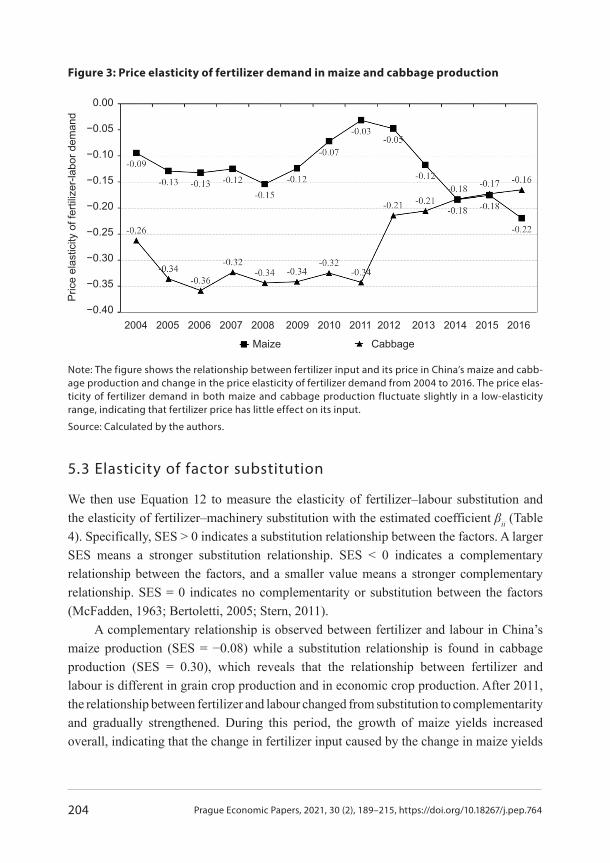
5.2 Price elasticity of fertilizer demand

We then use Equation 11 to measure the price elasticity of fertilizer demand in China’s maize and cabbage production (reported in Table 4) with the estimated coefficient βii and the corresponding cost share data. Figure 3 shows the change in elasticity of fertilizer demand over time: the elasticities of fertilizer demand of two crops are less than 0. The results indicate that fertilizer input declines with increasing fertilizer price. Hence, the government may increase fertilizer prices to reduce fertilizer use in crop production.


From the perspective of the elasticity value, the fertilizer demand elasticities for maize and cabbage are −0.12 and −0.29, respectively, which is in the range of inelasticity. According to changing trends, the elasticity of fertilizer demand fluctuates slightly in the inelastic range. The results indicate that fertilizer is a necessity in agricultural production, the space for fertilizer demand changing with the price is highly limited, and the effect of adjusting fertilizer input by adjusting fertilizer price is minimal.

Table 4: Price elasticity of demand and elasticity of factor substitution (2004–2016)

Price elasticity of demand Elasticity of factor substitution

Fertilizer Fertilizer – labour Fertilizer – machinery

Maize −0.1169 −0.0831 0.7038

Cabbage −0.2785 0.2985 −0.5408

Note: Long-term averages of elasticities are listed in the table. The price elasticity of demand was measu-red using Equation 11, and the elasticity of factor substitution was measured using Equation 12.


From the perspective of the difference between maize and cabbage (Figure 3), the average price elasticity of fertilizer demand in cabbage production is higher than that in maize production, and fertilizer inputs of cabbage are more sensitive to price changes to a certain extent; this result means that fertilizer is more important to grain crops than to economic crops. The reason may be that the production of economic crops is closely connected with the market, and their price is strongly determined by the market; producers of economic crops are highly sensitive to price changes on the market. While the production target of grain crops is always to continuously increase production to ensure national food security; under the action of the policy of grain purchase price protection, its factor demand is less sensitive to changes in market price. Besides, the price elasticity of maize fertilizer demand has shown a growth trend since 2011; in contrast, the price elasticity of cabbage fertilizer demand always shows a downward trend. One possible reason is the related policies of grain growth and strengthened agricultural environment governance in the National Modern Agriculture Development Plan (2011–2015). This event was promulgated by the State Council in 2011 during the 12th five-year period.


Figure 3: Price elasticity of fertilizer demand in maize and cabbage production

Note: The figure shows the relationship between fertilizer input and its price in China’s maize and cabb-age production and change in the price elasticity of fertilizer demand from 2004 to 2016. The price elas-ticity of fertilizer demand in both maize and cabbage production fluctuate slightly in a low-elasticity range, indicating that fertilizer price has little effect on its input.


5.3 Elasticity of factor substitution

We then use Equation 12 to measure the elasticity of fertilizer–labour substitution and the elasticity of fertilizer–machinery substitution with the estimated coefficient βii (Table 4). Specifically, SES > 0 indicates a substitution relationship between the factors. A larger SES means a stronger substitution relationship. SES < 0 indicates a complementary relationship between the factors, and a smaller value means a stronger complementary relationship. SES = 0 indicates no complementarity or substitution between the factors (McFadden, 1963; Bertoletti, 2005; Stern, 2011).

A complementary relationship is observed between fertilizer and labour in China’s maize production (SES = −0.08) while a substitution relationship is found in cabbage production (SES = 0.30), which reveals that the relationship between fertilizer and labour is different in grain crop production and in economic crop production. After 2011, the relationship between fertilizer and labour changed from substitution to complementarity and gradually strengthened. During this period, the growth of maize yields increased overall, indicating that the change in fertilizer input caused by the change in maize yields

0.00

−0.05

−0.10

−0.15

−0.20

−0.25

−0.30

−0.35

−0.40 2004 2005 2006 2007 2008 2009 2010 2011 2012 2013 2014 2015 2016

CabbageMaize

Pric

e el

astic

ity o

f fer

tiliz

er-la

bor d

eman

d


had no significant impact on the elasticity of fertilizer–labour substitution (Figure 4). In the future, the labour price in China will continue to rise due to the gradual elimination of the demographic dividend. This event will reduce fertilizer input in China’s current maize production to some extent but has no impact on fertilizer input in China’s current cabbage production.

Figure 4: Elasticity of fertilizer–labour substitution in maize and cabbage production

Note: The figure shows the relationship between fertilizer input and labour input in China’s maize and cabbage production and its change from 2004 to 2016. There is a substitution relationship between fertilizer input and labour input in cabbage production and it shows a weakening trend; the relationship between fertilizer input and labour input in maize production changes from substitution to complemen-tarity, and the complementary relationship shows an enhancement trend.


A strong substitution relationship exists between fertilizer and machinery in China’s maize production (SES = 0.70), whereas the relationship between fertilizer and machinery was strongly complementary in China’s cabbage production (SES = −0.54), showing that the relationship between fertilizer and machinery is different in grain crop production and in economic crop production. Figure 5 shows that over time, the intensity of the substitution relationship between fertilizer and machinery exhibits a slowly declining trend. However, the value of elasticity of substitution is always greater than 0.5, indicating that fertilizer input is excessive and machinery input is insufficient in maize production. The marginal

2004 2005 2006 2007 2008 2009 2010 2011 2012 2013 2014 2015 2016

CabbageMaize

0.6

0.5

0.4

0.3

0.2

0.1

0

−0.1

−0.2

−0.3

−0.4

Ela

stic

ity o

f fer

tiliz

er-la

bor s

ubst

itutio

n


revenue of adding a unit of machinery is higher than that of adding a unit of fertilizer. Hence, when the price of agricultural machinery falls induced by agricultural machinery subsidy policy, farmers choose to increase machinery input and reduce fertilizer input at the same time. When the price of agricultural machinery rises, farmers can reduce machinery input and rely on increasing fertilizer input to ensure production. As a suburban agriculture type, the cabbage growing scale is smaller than that of field crops such as rice, wheat, and maize with regard to the complementary relationship between fertilizers and machinery in cabbage production. Thus, large-scale mechanized production cannot be carried out. The promotion effect of machinery in cabbage production is mainly reflected in intensive operation using a fertilizer application machine to assist fertilization as a factor replacement for labour. The government can reduce the price of machinery used in maize production and increase the price of machinery used in cabbage production via price policy to reduce fertilizer input.

Figure 5: elasticity of fertilizer–machinery substitution in maize and cabbage

production

Note: The figure shows the relationship between fertilizer input and machinery input in China’s maize and cabbage production and its change from 2004 to 2016. There is a substitution relationship between fertilizer input and machinery input in maize production and it shows a weakening trend; and there is a complementary relationship between fertilizer input and machinery input in cabbage production and it shows a weakening trend as well.


2004 2005 2006 2007 2008 2009 2010 2011 2012 2013 2014 2015 2016

1.2

0.9

0.6

0.3

0

−0.3

−0.6

−0.9

−1.2

CabbageMaize

Ela

stic

ity o

f fer

tiliz

er-m

achi

nery

sub

stitu

tion


6. Conclusions and Discussion

This study constructed a translog cost function model and a SES model using factor input and price data from 2004 to 2016, and applied a SUR approach to measure the price elasticity of fertilizer demand and the elasticity of factor substitution in China’s maize and cabbage production. The results reveals that (1) the input and price of all the factors have a significant influence on fertilizer share in maize production, and fertilizer price has a significant influence on fertilizer share in cabbage production; (2) the elasticity of fertilizer demand is in a low-elasticity range, the price elasticity of fertilizer demand of cabbage is higher than that of maize; (3) there is a complementary relationship between fertilizer and labour and a substitution relationship between fertilizer and machinery in China’s maize production, while these relationships are opposite in China’s cabbage production; (4) from a general point of view, fertilizer is a necessity in both grain crop and economic crop production, while the substitution relationships between different agricultural input factors, such as fertilizer and labour, fertilizer and machinery, are different in grain crop production and in economic crop production.

Our findings have the following policy implications. (1) The government should deliberate whether to reduce fertilizer use by raising the price of fertilizers. The low price elasticity of fertilizer demand makes it difficult for the government to reduce fertilizer input via price policy even if the price of fertilizer is greatly increased; meanwhile, high price of fertilizers would increase households’ planting costs. It would be a better choice for the government to use a stable price policy and mainly use non-price policy to control fertilizer use. (2) The government can adjust the price of agricultural machinery to regulate fertilizer input. Subsidizing the machinery needed for agricultural production can effectively reduce fertilizer input. (3) The government can strengthen the investment in education and skill training of agricultural labour force and cultivate new types of agricultural talents.

This study contributes to research on fertilizer use in agricultural production by providing latest empirical evidence in the case of China, the world’s largest developing country and a major agricultural producing country. We focused on the price of fertilizer and other agricultural input factors of representative crops; the research findings present explanations from the perspectives of price elasticity of demand and elasticity of substitution, which supplement two streams of literature: the influencing factors of fertilizer input and elasticity of agricultural input factors. Furthermore, we obtained the price elasticity of fertilizer demand and substitution elasticity of agricultural production factors in the empirical analysis; thus, this study enriches the practical application of microeconomic factor demand theory. Finally, our research conclusions


not only have explanatory power in China, but also contribute to other large agricultural countries and developing countries, for whom our research results will offer references to grasp the relationship between input factors (represented by fertilizer) in agricultural production, thereby planning and adjusting agricultural production strategies based on local conditions and crop conditions. Meanwhile, the results-based policy implications may help countries facing serious agricultural non-point source pollution by providing suggestions to formulate agricultural environmental policies rationally. Therefore, this study makes a contribution to promoting the world’s reasonable and efficient fertilizer use and sustainable development of agricultural production.

This study admittedly has the following limitations. Firstly, the area and crop varieties that the sample can cover are limited due to data size limitations; as a result, there is a lack of heterogeneity analysis and international comparative research in this study. Secondly, as we used aggregate data, the empirical analysis was made at the province level. Since we cannot examine fertilizer use and agricultural production decisions from the perspective of households and individuals, the influence channels and mechanisms of the price effect and factor substitution effect on fertilizer use have not been fully discussed. In the future, based on data improvements, we will further use micro-investigation data to examine the specific impact paths and mechanisms of households’ fertilizer use and agricultural production decisions. In addition, we will focus on heterogeneity analysis of different regions within China, different countries and different crops, and accordingly offer policy recommendations with more global value.

Appendix

Appendix A.1

Binswanger (1974), and Koesler and Schymura (2014) provided the AES formula based on the parameter estimation results of Equation 9:

ij i j

iji j

S SS S

, i ≠ j

2

2

ii i i

iji

S SS

, i = j (A.1)


The MES describes the variation of the factor j’s price (Pj) on the change rate (Xi / Xj) of the factor i’s input (Xi) relative to the factor j’s input (Xj) under the output level and other factor prices remaining unchanged (Morishima, 1974; Karney, 2016):

ln( / ) ( )

lnij ij i jM

ij ji j i

C C X XP

C C P

(A.2)

Comparing Equations A.1, A.2, and 10, the SES definitions are closer to Hicks’ definitions of elasticity of substitution, and their estimated results are more robust under different forms of translog cost functions compared with the AES and MES (Stern, 2011; Hao, 2015).

Appendix A.2

Table A.1: Fertilizer input in some countries/regions in 2016

Countries (regions)Fertilizer input

(ten kilo-tonnes)

Average fertilizer input

(kg/ha)

China 5,331.21 453.58

United States (US) 2,054.40 128.49

Canada 382.50 98.82

Japan 103.00 230.37

European Union (EU) 1,688.05 139.61

Asia 10,777.13 184.21

World 18,721.01 119.98

Note: The fertilizer input describes the countries/regions’ total amount of fertilizer used in agricultu-ral production, and the average fertilizer input describes the countries/regions’ fertilization intensity in agricultural production, which is closely related to the environmental pollution.

Source: Food and Agriculture Organization of the United Nations (FAO) dataset.


Table A.2: Year dummy estimated results from the maize cost share function



2005 0.0094 ** 0.0040 0.0331 *** 0.0109 −0.0020 0.0044

2006 −0.0037 0.0045 0.0586 *** 0.0123 0.0018 0.0050

2007 −0.0104 * 0.0060 0.0805 *** 0.0166 −0.0004 0.0067

2008 0.0226 ** 0.0104 0.0979 *** 0.0286 −0.0077 0.0115

2009 −0.0123 0.0100 0.1301 *** 0.0277 −0.0093 0.0111

2010 −0.0392 *** 0.0112 0.1760 *** 0.0309 −0.0124 0.0124

2011 −0.0376 *** 0.0145 0.2208 *** 0.0400 −0.0209 0.0162

2012 −0.0529 *** 0.0162 0.2846 *** 0.0447 −0.0238 0.0181

2013 −0.0680 *** 0.0173 0.3201 *** 0.0478 −0.0292 0.0193

2014 −0.0887*** 0.0176 0.3553 *** 0.0484 −0.0260 0.0196

2015 −0.0871 *** 0.0182 0.3608 *** 0.0501 −0.0178 0.0203

2016 −0.0991 *** 0.0187 0.3397 *** 0.0516 −0.0262 0.0208

Note: We use White’s heteroskedasticity-robust standard errors in the SUR to avoid the non-spherical perturbation; *** p < 0.01, ** p < 0.05, * p < 0.1.Source: Calculated by the authors.

Table A.3: Year dummy estimated results from the cabbage cost share function



2005 0.0130 0.0079 −0.0145 0.0229 0.0094 ** 0.0046

2006 −0.0068 0.0083 0.0048 0.0241 0.0066 0.0049

2007 −0.0226 ** 0.0105 0.0081 0.0307 0.0103 * 0.0062

2008 −0.0039 0.0205 −0.0089 0.0596 0.0368 *** 0.0121

2009 −0.0358 * 0.0187 0.0163 0.0542 0.0339 *** 0.0110

2010 −0.0607 *** 0.0203 0.0666 0.0591 0.0322 *** 0.1201

2011 −0.0570 ** 0.0270 0.0831 0.0784 0.0428 *** 0.0159

2012 −0.0833 *** 0.0303 0.1217 0.0883 0.0505 *** 0.0179

2013 −0.1022 *** 0.0316 0.1413 0.0920 0.0430 ** 0.0187

2014 −0.1183 *** 0.0310 0.1765 * 0.0904 0.0422 ** 0.0183

2015 −0.1201 *** 0.0320 0.1937 ** 0.0930 0.0378 ** 0.0189

2016 −0.1334 *** 0.0322 0.1969 ** 0.0938 0.0316 * 0.0190

Note: We use White’s heteroskedasticity-robust standard errors in the SUR to avoid the non-spherical perturbation; *** p < 0.01, ** p < 0.05, * p < 0.1.Source: Calculated by the authors.


Table A.4: Province dummy estimated results from the maize cost share function



Inner Mongolia −0.0413 0.0268 0.1203 0.0737 0.0147 0.0298

Jilin −0.0153 0.0227 0.1510 ** 0.0626 −0.0091 0.0252

Sichuan 0.0002 0.0072 0.0520 *** 0.0198 0.0089 0.0081

Ningxia 0.0001 0.0142 0.1477 *** 0.0390 −0.0054 0.0150

Anhui 0.0177 0.0161 0.1264 *** 0.0443 −0.0016 0.0179

Shandong 0.0268 0.0190 0.1273 ** 0.0522 0.0288 0.0211

Shanxi −0.0237 0.0269 0.1953 *** 0.0739 0.0375 0.0298

Guangxi −0.0034 0.0118 0.0903 *** 0.0323 −0.0308 ** 0.0131

Xinjiang −0.0487 0.0460 0.3453 *** 0.1265 −0.0083 0.0512

Jiangsu 0.0105 0.0190 0.1829 *** 0.0536 −0.0262 0.0216

Hebei −0.0238 0.0089 0.1766 ** 0.0815 0.0393 0.0329

Henan −0.0010 0.0138 0.0852 0.0523 0.0233 0.0211

Hubei 0.0187 ** 0.0075 0.0689 *** 0.0245 −0.0220 ** 0.0099

Gansu −0.0284 ** 0.0145 0.0613 0.0381 0.0213 0.0154

Guizhou 0.0146 * 0.0057 0.0186 0.0207 −0.0008 0.0084

Liaoning −0.0102 0.0234 0.0204 0.0401 −0.0122 0.0162

Chongqing 0.0160 *** 0.0288 0.0259 0.0159 0.0026 0.0064

Shaanxi −0.0238 0.0546 0.2366 *** 0.0645 0.0313 0.0260

Heilongjiang −0.0221 0.0458 0.1132 0.0793 0.0230 0.0320

Note: We use White’s heteroskedasticity-robust standard errors in the SUR to avoid the non-spherical perturbation; *** p < 0.01, ** p < 0.05, * p < 0.1.



Table A.5: Province dummy estimated results from the cabbage cost share function



Xinjiang −0.0266 0.0169 −0.0971 ** 0.0493 0.0345 *** 0.0100

Gansu 0.2431 *** 0.0457 0.2357 * 0.1331 −0.1566 *** 0.0207

Jiangsu 0.0636 *** 0.0198 0.0836 0.0576 −0.0589 *** 0.0117

Jiangxi 0.1800 *** 0.0364 0.2760 *** 0.0106 −0.1212 *** 0.0215

Fujian 0.2041 *** 0.0489 0.0686 0.1423 −0.1813 *** 0.0289

Inner Mongolia 0.1282 *** 0.0318 0.1020 0.0926 −0.1323 *** 0.0188

Tianjin 0.0725*** 0.0184 0.1854 *** 0.0537 −0.0786 *** 0.0109

Zhejiang 0.0443*** 0.0145 0.0953 ** 0.4205 0.0419 *** 0.0085

Yunnan 0.1584 *** 0.0372 0.1366 0.1083 −0.1221 *** 0.0220

Hubei 0.1762 *** 0.0366 0.2152 ** 0.1062 −0.1486 *** 0.0216

Shandong 0.0443 *** 0.0087 0.0561 ** 0.0253 −0.0159 *** 0.0051

Qinghai 0.1747 *** 0.0427 0.2653 ** 0.1241 −0.1775 *** 0.0252

Chongqing 0.2235 *** 0.0480 0.3188 ** 0.1396 −0.1744 *** 0.0283

Ningxia 0.0917 *** 0.0222 0.1265 * 0.1023 −0.0879 *** 0.0131

Liaoning 0.1342 *** 0.0352 0.1429 0.0647 −0.1083 *** 0.0207

Note: We use White’s heteroskedasticity-robust standard errors in the SUR to avoid the non-spherical perturbation; *** p < 0.01, ** p < 0.05, * p < 0.1.


References

Abdoulaye, T., Sanders, J. H. (2015). Stages and Determinants of Fertilizer Use in Semiarid African Agriculture: the Niger Experience. Agricultural Economics, 32(2), 167–179, http://doi.org/10.1111/j.0169-5150.2005.00011.x

Bertoletti, P. (2005). Elasticities of Substitution and Complementarity: A Synthesis. Journal of Productivity Analysis, 24(2), 183–196, http://doi.org/10.2307/41770200

Binswanger, H. P. (1974). A Cost Function Approach to the Measurement of Elasticities of Factor Demand and Elasticities of Substitution. American Journal of Agricultural Economics, 56(2), 377–386, http://doi.org/10.2307/1238771


Chen, S. Z., Song, C. X., Song, N., et al. (2013). Chinese Wheat Production Technology Progress and Factor Demand and Substitution Behavior. Chinese Rural Economy, 9, 18–30.

Clark, J. S., Cechura, L., Thibodeau, D. R. (2013). Simultaneous Estimation of Cost and Distance Function Share Equations. Canadian Journal of Agricultural Economics, 61(4), 559–581, http://doi.org/10.1111/j.1744-7976.2012.01269.x

Dawson, C. J., Hilton, J. (2012). Fertilizer Availability in a Resource-limited World: Production and Recycling of Nitrogen and Phosphorus. Food Policy, 36(1), S14–S22, http://doi.org/10.1016/j.foodpol.2010.11.012

Du, N., Shao, Q. Q., Hu, R. F. (2019). Price Elasticity of Production Factors in Beijing’s Picking Gardens. Sustainability, 11(7), 2160, http://doi.org/10.3390/su11072160

Duan, P. L., Qin, L. J., Wang, Y. Q., et al. (2016). Spatial Pattern Characteristics of Water Footprint for Maize Production in Northeast China. Journal of the Science of Food and Agriculture, 96(2), 561–568, http://doi.org/10.1002/jsfa.7124

Gao, D. M., Wang, L. H., Tian, Z. H. (2018). Research on the Factor Substitution Relationships of Wheat Production. Journal of China Agricultural University, 23(6), 169–176, http://doi.org/10.11481/j.issn.1007-4333.2018.06.19

Greene, W. H. (2017). Econometric Analysis. US: Pearson Publisher.

Guilkey, D. K. (1974). Alternative Tests for a First-order Vector Autoregressive Error Specification. Journal of Econometrics, 2(1), 95–104, http://doi.org/10.1016/0304-4076(74)90032-3

Hao, F. (2015). Formula Correction and Estimation Methods Comparison on Elasticity of Substitution within Translog Functions. The Journal of Quantitative & Technical Economics, 32(4), 89–106, http://doi.org/10.13653/j.cnki.jqte.2015.04.006

Henderson, D. J., Kumbhakar, S. C., Li, Q., et al. (2015). Smooth Coefficient Estimation of a Seemingly Unrelated Regression. Journal of Econometrics, 189(1), 148–162, http://doi.org/10.1016/j.jeconom.2015.07.002

Hu, H., Yang, Y. B. (2015). Research on Fertilizer Application of Rural Households from the Perspective of Factor Substitution: Based on Rural Household Data from Fixed Observation Points in Rural Areas. Journal of Agrotechnical, 239(3), 86–93, http://doi.org/10.13246/j.cnki.jae.2015.03.009

Ju, X. T., Gu, B. J., Wu, Y. Y., et al. (2016). Reducing China’s Fertilizer Use by Increasing Farm Size. Global Environmental Change, 41, 26–32, https://doi.org/10.1016/j.gloenvcha.2016.08.005

Karney, D. H. (2016). General Equilibrium Models with Morishima Elasticities of Substitution in Production. Economic Modelling, 53, 266–277, http://doi.org/10.1016/j.econmod.2015.12.003

Kim, D. G., Shim, J. Y., Ko, M. J., et al. (2018). Statistical Modeling for Estimating Glucosinolate Content in Chinese Cabbage by Growth Conditions. Journal of the Science of Food and Agriculture, 98(9), 3580–3587, http://doi.org/10.1002/jsfa.8874


Kitenge, E. (2016). Effects of Food and Agricultural Imports on Domestic Factors in the U.S. Agricultural Sector: a Translog Cost Function Framework. Applied Economics Letters, 23(2), 132–137, http://doi.org/10.1080/13504851.2015.1058897

Koesler, S., Schymura, M. (2015). Substitution Elasticities in a Constant Elasticity of Substitution Framework: Empirical Estimates Using Nonlinear Least Squares. Economic Systems Research, 27(1), 101–121, http://doi.org/10.1080/09535314.2014.926266

Lin, B. Q., Atsagli, P. (2017). Inter-fuel Substitution Possibilities in South Africa: A Translog Production Function Approach. Energy, 121, 822–831, http://doi.org/10.1016/j.energy.2016.12.119

Lin, B. Q., Tian, P. (2016). The Energy Rebound Effect in China’s Light Industry: a Translog Cost Function Approach. Journal of Cleaner Production, 112, 2793–2801, http://doi.org/10.1016/j.jclepro.2015.06.061

Liu, Y. M., Hu, W. Y., Jette-Nantel, S., et al. (2014). The Influence of Labor Price Change on Agricultural Machinery Usage in Chinese Agriculture. Canadian Journal of Agricultural Economics, 62(2), 219–243, http://doi.org/10.1111/cjag.12024

Liu, Z. G., Zhao, Y., Guo, S., et al. (2019). Enhanced Crown Root Number and Length Confers Potential for Yield Improvement and Fertilizer Reduction in Nitrogen-efficient Maize Cultivars. Field Crops Research, 241, 107562, http://doi.org/https://doi.org/10.1016/j.fcr.2019.107562

Lu, H., Xie, H. L., He, Y. F., et al. (2018). Assessing the Impacts of Land Fragmentation and Plot Size on Yields and Costs: A Translog Production Model and Cost Function Approach. Agricultural Systems, 161, 81–88, http://doi.org/10.1016/j.agsy.2018.01.001

Ma, L., Long, H. L., Zhang, Y. N., et al. (2019). Agricultural Labor Changes and Agricultural Economic Development in China and Their Implications for Rural Vitalization. Journal of Geographical Sciences, 29(2), 163–179, http://doi.org/10.1007/s11442-019-1590-5

Ma, W. L., Abdulai, A., Goetz, R. (2018). Agricultural Cooperatives and Investment in Organic Soil Amendments and Chemical Fertilizer in China. American Journal of Agricultural Economics, 100(2), 502–520, http://doi.org/10.1093/ajae/aax079

McFadden, D. (1963). Constant Elasticity of Substitution production functions. Review of Economic Studies, 30(2), 73–83, http://doi.org/10.2307/2295804

McKeown, A. W., Westerveld, S. M., Bakker, C. J. (2010). Nitrogen and Water Requirements of Fertigated Cabbage in Ontario. Canadian Journal of Plant Science, 90, 101–109, https://doi.org/10.4141/CJPS09028

Mustapha, A. B., Said, R. (2016). Factors Influencing Fertilizer Demand in Developing Countries: Evidence from Malawi. Journal of Agribusiness in Developing & Emerging Economies, 6(1), 59–71, http://doi.org/10.1108/JADEE-10-2013-0040

National Bureau of Statistics of China (2017). China Statistical Yearbook. China: China Statistics Press. ISBN 978-7-5037-8253-4.

National Development and Reform Commission of China (2017). National Agricultural Cost–Benefit Data Compilation. China: China Statistics Press. ISBN 978-7-5037-8233-6.


Sheng, Y., Ding, J. P., Huang, J. K. (2019). The Relationship between Farm Size and Productivity in Agriculture: Evidence from Maize Production in Northern China. American Journal of Agricultural Economics, 101(3), 790–806, http://doi.org/10.1093/ajae/aay104

Stern, D. I. (2011). Elasticities of Substitution and Complementarity. Journal of Productivity Analysis, 36(1), 79–89, http://doi.org/10.1007/s11123-010-0203-1

Su, X. M., Zhou, W. S., Nakagami, K., et al. (2012). Capital Stock-labor-energy Substitution and Production Efficiency Study for China. Energy Economics, 34(4), 1208–1213, http://doi.org/10.1016/j.eneco.2011.11.002

Takeshima, H., Nkonya, E. (2014). Government Fertilizer Subsidy and Commercial Sector Fertilizer Demand: Evidence from the Federal Market Stabilization Program (FMSP) in Nigeria. Food Policy, 47, 1–12, http://doi.org/10.1016/j.foodpol.2014.04.009

Tian, Y., Zhang, J. B., He, K., et al. (2015). Analysis on the Low Carbon Production Behavior of Farmers and its Influencing Factors: Taking Fertilizer Application and Pesticide Use as Examples. China Rural Survey, 4, 61–70.

Wang, L., Gao, L., Zhang, W. F., et al. (2008). Evaluation of Environment of Chemical Fertilizer Industry in China and Analysis of International Competitiveness. Chemical Fertilizer Industry, 35(6), 16–21.

Wang, Z. L., Xiao, H. F. (2008). Analysis of the Effect of Fertilizer Application on Grain Yield Growth. Issues in Agricultural Economy, 8, 65–68, http://doi.org/10.13246/j.cnki.iae.2008.08.012

Woodland, A. D. (1975). Substitution of Structures, Equipment and Labor in Canadian Production. International Economic Review, 16(1), 171–187, http://doi.org/10.2307/2525892

Wu, Y. (2011). Chemical Fertilizer Use Efficiency and its Determinants in China’s Farming Sector: Implications for Environmental Protection. China Agricultural Economic Review, 3(2), 117–130, http://doi.org/10.1108/17561371111131272

Xiang, Y. Z., Zou, H. Y., Zhang, F. C., et al. (2018). Effect of Irrigation Level and Irrigation Frequency on the Growth of Mini Chinese Cabbage and Residual Soil Nitrate Nitrogen. Sustainability, 11(1), 111, http://doi.org/10.3390/su11010111

Xiong, Y., Wu, J. (2017). Zero Growth of Fertilizer: Review and Revelation. Environmental Protection, 18, 57–60, http://doi.org/10.14026/j.cnki.0253-9705.20170924.001

Zha, D. L., Ding, N. (2014). Elasticities of Substitution between Energy and Non-energy Inputs in China Power Sector. Economic Modelling, 38, 564–571, https://doi.org/10.1016/j.econmod.2014.02.006

Documents

Elasticity of Substitution, Price Effect and Sustainable