Embed Size (px)
Citation preview

NBER WORKING PAPER SERIES
ESTIMATING MODELS WITHINTERTEMPORAL SUBSTITUTION USING
AGGREGATE TIME SERIES DATA
Martin S. Eichenbaum
Lars Peter Hansen
Working Paper No. 2181
NATIONAL BUREAU OF ECONOMIC RESEARCH1050 Massachusetts Avenue
Cambridge, MA 02138March 1987
An earlier version of this research was presented at the NationalBureau of Economic Research meetings on Economic Fluctuations,November 1983. This research was supported by grants from theNational Science Foundation and the Sloan Foundation. Helpfulcomments were made by John Heaton, Joe Hotz, Dale Jorgenson,Barbara Mace, Masao Ogaki, and Grace Tsaing. The research reportedhere is part of the NBER's research program in Economic FluctuationsAny opinions expressed are those of the authors and not those ofthe National Bureau of Economic Research.

NBER Working Paper #2181March 1987
Estimating Models with Intertemporal SubstitutionUsing Aggregate Time Series Data
ABSTRACT
In conducting empirical investigations of the permanent income model ofconsumption and the consumption-based intertemporal asset pricing model,various authors have imposed restrictions on the nature of thesubstitutability of consumption across goods and over time. In this paper wesuggest a method for testing some of these restrictions and presentempirical results using this approach. Our empirical analyses focuses onthree questions: (1) Can the services from durable and nondurable goods betreated as perfect substitutes? (ii) Are preferences completely separablebetween durable and nondurable goods? (iii) What is the nature ofintertemporal substitutability of nondurable consumption? When consumers'preferences are assumed to be quadratic, there is very little evidenceagainst the hypothesis that the services from durable goods and nondurablegoods are perfect substitutes. These results call into question the practiceof testing quadratic models of aggregate consumption using data onnondurables and services only. When we consider S branch specifications,we find more evidence against perfect substitutability between serviceflows, but less evidence against strict separability across durable andnondurable consumption goods. Among other things, these findings suggestthat the empirical shortcomings of the intertemporal asset pricing modelcannot be attributed to the neglect of durable goods.
Martin Eichenbaum Lars Peter HansenGraduate School of Department of EconomicsIndustrial Administration University of ChicagoCarnegie Mellon University Chicago, Ii 60637Pittsburgh, P.A. 15213

INTRODUCTIONIn conducting empirical investigations of the permanent income model of
consumption and the consumption-based interternporal asset pricing model.,various authors have imposed restrictions on the nature of the substitutability ofconsumption across goods and over time. The purpose of this paper is tosuggest a method for testing some of these restrictions and to present empiricalresults using this approach. Our empirical analysis focuses on three questions:
(1) Can the services from durable and nondurable consumption goods be treatedas perfect substitutes?
(ii) Are preferences completely separable between durable and nondurableconsumption goods?
(iii) What is the nature of intertemporal substitutability of nondurableconsumption?
Several researchers have added the services from durables to nondurables toform a composite time series on consumption [e.g. see Darby (1975) and Sargent(1978)1. A justification for this practice is that the answer to question (I) isyes. Other researchers have ignored durables when studying models of aggregateconsumption and asset returns [e.g. see Hall (1978), Flavin (1981), Grossmanand Shiller (1981), and Hansen and Singleton (1982,1983)). A justification forthis practice is that the answer to question (ii) is yes. The third question is ofinterest because Sims (1980) and Novales (1986) have suggested that the usual
practice of modeling nondurable consumption goods as being time separable maybe inapproriate when studying the co-movements of consumption and interestrates. They argue that consumers may face adjustment costs in changing theirconsumption patterns as suggested by Houthakkar and Taylor (1970). Acompeting hypothesis is that what are classified as nondurable goods formeasurement purposes have some degree of durability.

2
To investigate these questions, we use a class of empirically tractablemodels of aggregate expenditures on consumption goods, relative prices, and
asset returns. In the models we consider, consumers solve dynamic optimization
problems subject to lifetime budget constraints. Real interest rates are allowedto vary over time. Since the consumers face an environment with uncertainty,they have incentives to trade assets other than riskiess securities, e.g.equities. Some of the goods which consumers can purchase are durable. Wefollow Peck (1970) in modeling durable goods as assets that generateconsumption services (dividends) in current as well as subsequent time periods.Consequently, intertemporal asset pricing theory can be used to deduce durablegoods prices in the same way that the prices of equities paying dividends incurrent and future time periods are deduced. The formal theoretical underpin-nings of the models we consider are given in Eichenbaurn, Hansen, and Richard(1984) and Hansen (1987). Those papers derive equilibrium relations betweenvariables such as aggregate expenditures on goods, relative prices of goods, andprices of other securities. The resulting class of empirical models is suffi-ciently broad to encompass many of the empirical models that have been used todate.
In our empirical analysis, it is necessary to maintain a set of auxiliaryassumptions. We maintain three types of assumptions: functional formrestrictions on the preferences over service flows from consumption goods,functional form restrictions on the form of the nonseparabilities over time, andrestrictions on growth in prices and aggregate quantities.
We use functional forms for consumers' preferences over service flows thatsatisfy two criteria. First, they rationalize the existence of a representativeconsumer in the sense of Gorman (1953). Second, they nest, as special cases,many of the preference specifications which have been used in the literature.The first criterion is imposed for tractability so that equilibrium prices do notdepend on the initial distribution of resources among consumers in the economy.Furthermore, the three empirical questions of interest translate directly fromproperties of the preferences of the individual consumers to properties of thepreferences of the corresponding representative consumer.

3
We model nonseparabilities over time in preferences for consumption goods
by viewing consumption goods as risk-free claims to consumption services in
current and future time periods. Hence, consumption goods are intemporalbundles of consumption services. These goods are priced in terms of prices ofthe consumption service streams that they generate. Thus we are able to obtain
convenient representations for the prices of newly acquired consumption goods.While this model of temporal nonseparabilities is admittedly extreme, it servesas an important benchmark for models in which utilization of durable goods isendogenized and/or private information and monitoring costs are introduced.Such extensions make the relation between the prices of consumer services and
the purchase prices of consumption goods considerably more complicated.Consequently, our benchmark model has many computational advantages overthese other models.
In this paper we abstract from modeling explicitly the production of newconsumption goods. Instead, we allow for relatively general processes forequilibrium consumption. We do, however, take an explicit stand on the impactof economic growth and technological progress on the equilibrium prices and
quantities. In so doing, it is important that we model growth in prices andquantities in a way that is internally consistent and allows for statisticallyconsistent estimation of parameters governing substitution across goods andover time. We consider two specifications of growth that have been commonlyused in applied time series analyses. One is a model in which geometricdetrending induces stationarity, and the other is a model in which logarithmicdifferencing induces stationarity. Each of these approaches has some advantagesand disadvantages. The first approach allows for more general specifications ofpreferences and service technologies. The second approach allows for additionalforms of growth but can only be used for a smaller set of preferences andGorman-Lancaster technologies. Both approaches imply a set of testablerestrictions across the growth rates in quantities and prices.
As a practical matter, we can use only a limited array of prices onconsumption goods and assets to estimate preference parameters and testrestrictions. Conventional approaches used in consumer demand theory such asestimating demand functions are not applicable to our setting.

4
Instead we follow an approach suggested by Hansen and Singleton (1982) andHansen and Richard (1987). This approach restricts the preference shockprocess of the fictitious representative consumer and exploits conditionalmoment representations of equilibrium prices to obtain a set of unconditionalmoment restrictions. We then use the generalized method of moments (GMM)methodology as developed by Hansen (1982) to estimate preference parametersand test the over-identifying unconditional moment restrictions. This approachdoes not require a complete set of data on prices or a complete specification ofthe conditioning information used by consumers. On the other hand, asimplemented in this paper, the approach does not permit unobservable timevarying preference shocks for the representative consumer and does not accountfor time aggregation in prices and quantities.
The remainder of this paper is organized as follows. In section one wepresent a version of the theoretical model analyzed by Eichenbaum, Hansen, andRichard (1984) and Hansen (1987) and describe the equilibrium processes foreconomy-wide averages of the multiple consumption goods. In section two wedisplay the equilibrium prices of claims to durable consumption goods and theimplied restrictions on the growth rates of quantities and prices. In sectionthree we show how to estimate parameters and test restrictions implied by themodel. In section four we report empirical results obtained using quadraticpreferences. In section five we report our empirical results using a version ofthe S branch utility Function suggested by Brown and Heien (1972). Finally, insection six we report our conclusions.

5
I. ThE MODEL
Eichenbaurn, Hansen, arid Richard (1984) analyzed an explicit equilibriummodel with heterogeneous consumers and multiple durable consumption goods.
They considered specifications of consumers' preferences and trading opportuni-ties that rationalize the existence of a representative consumer in the sense ofGorrnan (1953). Consequently, their model implies econometrically tractablerelations between aggregate consumption of durable goods, prices of durablegoods, and asset returns. In this section we describe briefly a particularversion of their economic model which accommodates growth.
A. INFORMATIONConsumers have a common sequence of information sets indexed by time.
Let 1(t) denote the set of information available to consumers at time t. Weassume that 1(t) is generated by {x(r) : r�t} where x(t) is a state vector at timet.
B. PREFERENCES
The preferences of consumers for durable goods are defined in two stages.First, preferences are defined over a vector of consumption services. Thesepreferences are separable over time and states. Then a dynamic Gorman-Lancaster technology is defined that maps acquisitions of durable consumptiongoods into current and future consumption services.
Let s3 (t) denote an rn-dimensional vector of services, and u- (t) denote an m-dimensional vector of shocks to consumer j's preferences at time t. Both s' (t)and uJ (t) are restricted to be in 1(t). At time zero, consumer j ranks alternative
consumption service processes using the utility function:
(1.1) (1/6c)E[ {U[s (t)-u (t)}U1flI(O)J
where ó (1-o) and

6
(i.2) Us(t)-u(t)) = { G{6[S1J(t)U1J(t)I}a)l/ai=1
The parameter 8 is a subjective discount factor between zero and one andnonnegative for each i. There are two branches of this utility functioncorresponding to whether o- is less than or greater than one. When o- is less thanone, a is less than or equal to one and U13 (t) can be viewed as a stochasticsubsistence point of consumer j for service I at time t. On the other hand, wheno- is greater than one, a is greater than or equal to one and u1 (t) can be viewedas a stochastic bliss point.
This specification of preferences is a version of the S branch utility function.Brown and Heien (1972) proposed the S branch utility function as ageneralization of the linear expenditure system, and used these preferences tostudy consumption behavior in a certainty environment. This class ofpreferences has a number of special cases, some of which we focus on in ourempirical analysis in section four. When a and a are the same, preferences arecompletely separable across the services in each time period and state. When ois less than one and a is zero, the function U has the Cobb-Douglas form:
(1.3) U[s3 (t) -Ui (t)J T{{6[sjJ (t) (t)J} e1
Finally, when both a and a are two, consumers' utility functions are quadratic.Several authors have used special cases of these preferences in studying
aggregate consumption behavior. For instance, Telser and Craves (1972), Hall(1978), Flavin (1981), and Mankiw (1982) use quadratic preferences in theirempirical analyses. Grossman and Shiller (1981) and Hansen and Singleton(1982, 1983) use a single consumption good version (m1) and consider valuesof ci that are less than one and subsistence points that are zero. Muellbauer(1981) uses a specification in which both o- and a are zero so that preferencesare logarithmically separable. Finally, Kydland and Prescott (1982) usepreferences with less than one and a equal to zero in which one of theconsumption services depends on current and past leisure.

7
Consumption goods are modeled as generating consumption services in currentand future time periods. It is convenient to represent the interternporalmapping from consumption goods into consumption services by introducinghousehold capital stocks. Let k3 (t- I) be a vector of household capital stocks ofconsumer j which are brought into time t. At time t consumer j augmentsthese stocks by a choice of n consumption goods which we denote c3 (t). Thetime t vector of household capital is then given by
(1 .4) k3 (t) = k3 (t- 1) + ®c (t)
for some matrices of real numbers i and ®. We restrict the matrix to haveeigenvalues that are strictly less than one in absolute value. The correspondingtime t consumption services are given by
(i.5) s3(t) = Fk3(t).
for some matrix F. Relations (1.4) and (1.5) can be used to construct a processfor consumption services (s3(t) : t=1,2,...} given an initial level k3(0) of thehousehold capital stocks and a process for consumption goods {c (t) : t1 ,2,..The matrices , 0, and F are assumed to be common across all consumers.
This mapping from consumption goods into consumption services can beviewed as a dynamic version of the household technology suggested by Gorman(1980) and Lancaster (1966). More precisely, consumption goods are bundledclaims to consumption services in current and future time periods since avector of consumption goods c(t) generates a vector of consumption servicesrtec(t) at time t+r for r0,1 Hence, the dynamic Gorrnan-Lancastertechnology induces time nonseparabilities into consumers' indirect preferencesfor goods. This form of nonseparabilities is consistent with specifications usedby Telser and Graves (1972) and Kydland and Prescott (1982).
One obvious rationale for (1.4) and (1.5) is that consumption goods aredurable and are purchased in order to augment the stocks of household capital. Inthis case the matrix dictates the rates at which the capital stocks depreciate.Specifications like (1.4) and (1.5) also appear in the consumer demand literature

8
where the household capital stocks are introduced to accommodate habitformation, adjustment costs in consumption, or committed consumptionexpenditures [e.g. see Houthakker and Taylor (1970), Pollack (1970), and Boyce(1975)].
C. EQUILIBRIUM CONSUMPTION PROCESSFor convenience, we calculate equilibrium prices as if the economy were an
endowment economy. The time t vector of the n economy-wide averages of newconsumption goods is denoted e*(t). The pricing relations we study also apply toeconomies In which new consumption goods are produced using intertemporaltechnologies with capital accumulation. For such economies e*(t) becomes thetime t average level of new consumption goods. The stochastic law of motionfor e*(t) can be calculated by solving an optimal resource allocation (Pareto)problem.1
Historical time series data on aggregate consumption and relative pricesdisplay pronounced growth. This complicates both model specification andeconometric estimation. Consistent estimation of substitution parameters is notfeasible with arbitrary patterns of growth. A common strategy is to modelgrowth so that there exist transformations for the time series data that inducestationarity. Such a strategy is adopted in this paper. Although we will notpresent a model in which growth is determined endogenously, we will be explicitabout the growth processes that are accommodated. We consider models ofgrowth that are consistent with two stationary-inducing transformations. Thefirst transformation entails logarithmic detrending and the second entails takingratios of variables (differencing logarithms). Each of these approaches has beenused extensively in applied time series analysis, and for our purposes, eachhas some distinct advantages and disadvantages.
Suppose the economy-wide average consumption of each good growsgeometrically over time. Let p1 denote the growth rate in consumption good ifor i = 1,2,...,n. Then,
(1.6) e*(t) = A(t) e(t)

9
for t�O where A(t) is a diagonal matrix with exp(p1t + in the 1th diagonalposition, e*(t) is the vector of unscaled equilibrium consumption goods, and e(t)is a vector of detrended equilibrium consumption goods with properties that willbe specified subsequently. Taking logarithms of (1.6) gives
(1.7) log[e*(t)J = + pt + logfe(t)J
where q5 and p are M-dimensional vectors with entries and p1 in theposition.
In our first model of growth, we assume that e(t) is a component of the statevector x(t) and the stochastic process {x(t) : -<t<+co} is strictly stationary.The parameter c is introduced for convenience so that
(1.8) E{log(e(t)1} = 0
Given the assumption of stationarity, (1.8) holds for all time periods.Suppose we take first differences of (1.7). Then
(1.9) loge*(t) - 1og[e*(t1)] = p + log[e(t)} - log[e(t-1)}
In our second model of growth we assume that log[e(t)1 - log[e(t-i)] is acomponent of x(t) where again {x(t) -a<t<+o} is a stationary stochastic process.The parameter p is identified by assuming that
(1.10) E{log[e(t)] — log[e(t—1)]} = 0
The components of this process have deterministic growth rates given by thecorresponding components of p, but the corresponding detrended process mustnow be treated differently to account for borderline nonstationarity in{log[e(t)1 : t�0}.

10
D. EQUILIBRIUM SERVICE PROCESS
To construct the economy-wide average level of consumption services inequilibrium, we let g(O) be the economy-wide average detrended vector ofhousehold capital stocks brought into the initial time period zero. Using (1.4)and (1.5), we define recursively
(1.11) g(t) = g(t—1) + ee(t)
and
(1.12) 1(t) = F'g(t)
for t=1,2%... where (1(t) : t�1} is the detrended economy-wide average
consumption service process and (g(t) : t�1} is the detrended economy-wideaverage process for household capital. These latter two processes inherit anyborderline nonstationarities in the equilibrium detrended consumption goodsprocess.
The preference specifications (1.1) and (1.2) and the time-invarianthousehold technology specification (1.4) and (1.5) are presumed to apply todetrended consumption goods and services. In appendix A we describespecifications of preferences and household service technologies that areconsistent with our analysis but apply to unscaled quantities.

:11
II. EQUILIBRIUM PRICES
Eichenbaum, Hansen, and Richard (1984) described alternative tradingopportunities that in conjunction with the specification of consumers'preferences are sufficient to rationalize a representative consumer version ofthe economy described in section one. The preferences of the representativeconsumer are given by (1.1) with the average preference shock u(t) replacingu(t). In our analysis we assume that all uncertainty with respect to individualpreference shocks is diversifiable. Hence we model u(t) as a constant u overtime.
For our purposes, it is most convenient to suppose that there are markets inexistence at some initial trading period for consumption services in each dateand state. This does not imply that trading must take place in all of thesemarkets to implement the equilibrium. Our focus is not on implementation butrather on the implied equilibrium prices. The introduction of markets inservices (or attributes) as opposed to goods simplifies our calculation ofequilibrium prices vis-a-vis standard analyses of static Gorman-Lancastertechnologies.
Given a rich collection of markets and preferences that are time and stateseparable, consumers have no incentives to engage in additional trading insubsequent time periods. Nevertheless, the equilibrium prices of consumptionservices in the initial trading period imply shadow prices of claims to new andused consumption goods that clear hypothetical markets in an economy withsequential trading opportunities. In this section, we report the equilibriumshadow prices. The interested reader is referred to Eichenbaum, Hansen, andRichard (1984) for a formal derivation of these results.
In representing the equilibrium prices we proceed in two steps. First weabstract from growth in consumption and represent equilibrium prices as if {e (t)
-co<t<+co} is the economy-wide average consumption process. We thenconsider the Implications of growth in the endowments for equilibrium prices.In particular, we use the equilibrium prices for the detrended quantities todeduce prices of the actual (unscaled) quantities. In this way growth in pricesand quantities is modeled in a manner that is internally consistent.

12
We first define the marginal utilities of a fictitious representative consumerand then use these marginal utilities to construct the equilibrium prices. Thetime t marginal utility vector of the hypothetical representative consumer ismu(t) = {mu1(t),mu2(t), ...,mum(t)]' where
(2.1) mu1 (t) (t)-u1]}t {e{[F (t) U1]}a}(-a)/a
These marginal utilities define the equilibrium prices of the consumptionservices. Since consumption goods are just bundled claims to consumptionservices, we can use these marginal utilities to construct the prices of newconsumption goods.
Let q(t) be the time t relative spot price vector of new consumption goods,and let the first element of the new consumption goods vector at time t be thenumeraire. Then
Ef r-t(J-,rte)/mu(r) 11(t))
(2.2) q(t) = rtEf V_t(FttGh)mu(r) 11(t)]
r=t
where h is a vector of zeroes except in the first position where there is a one.Notice that the numerator of the right-hand side of (2.2) is the discountedconsumption service flow generated by a vector of new consumption goods.Likewise, the denominator is the discounted service flow of the first newconsumption good at time t. The marginal utility vector enters both thenumerator and denominator as a stochastic discount factor.
Also, consider a security that pays off y(t+i) units of the first newconsumption good at time period t+1. The time t relative price of this security,
denoted ir[y(t+1),t}, is given by

13
Efy(t+1) tt(Ttti9h)/mu(r)tI(t)Jr=t+1
(2.3) iry(t+i),t) =E[ t_t(FATtêh)/mu(t)1I(tfl
r=t
As in (2.2), the numerator and denominator of the right-hand side of (2.3) arediscounted service flows.
We now use the equilibrium prices for the detrended quantites to deduceprices for the unscaled quantities. Let q*(t) be the vector of spot prices for theunscaled new consumption goods at time t. We take the first new unscaledconsumption good at time t to be the time t numeraire. Then the relationbetween q*(t) and q(t) is
(2.4) 1og[q(t)} = (41 - •) + (ptl - p)t + Log(q(tYl
where I is an M-dimensional vector of ones and q(t) is given by (2.2). In (2.4)the subtraction of c + pt adjusts for the transformation of quantities given in(1.7) and the addition of ptt + c ensures that the first unscaled new consumptiongood is nurneraire instead of the first detrended new consumption good.Similarly, let y(t+1) be the payoff on a security expressed in units of the firstunscaled consumption good, and let lr*1:y(t+ 1) ,t) be the time t price of thissecurity expressed in time t units of the first unscaled consumption good. Then
(2.5) lr*[y(t+1),t} = lr[y(t+1),tlexp[(t+1)J.4j + cPt — t/.Jt—
ir[y(t+1),t}exp(p)
where iry(t+1),t} is given in (2.3).
If e(t) and y(t) are components of the vector x(t) and {x(t) : -co<t<+x} is astationary process, then the price processes {q(t) : -<t<+co} and (ir{y(t+i),t)-<t<+co} are jointly stationary with {x(t) : -<t<+}. Since the process {q(t)-o<t<+co} is stationary, (2.4) gives a set of stationary-inducing transformationsfor equilibrium relative prices. Hence there is a set of restrictions implied onthe growth rates of prices and quantities. Among other things, these restrictionshave the testable implication that expenditures on each consumption good grow atthe same rate p.

14
If instead, only log[e(t)} - log[e(t-IY1 and y(t) are components of x(t) where
{x(t) : -<t<+} is a stationary process, then additional complications arise.While the economic model may still remain valid, in general there will not bea simple transformation, such as differencing logarithms of prices, that willinduce stationarity. For particular pararneterizations of our model., however,such differencing will in fact induce stationarity. Suppose u is zero, n = m, a =0 (so that U is Cobb-Douglas), and that each consumption service is generatedby a distinct consumption good so that Ftg is diagonal for all r�0. In thiscase the ratios of equilibrium consumption services to the correspondingconsumption goods are stationary. The equilibrium marginal utilities ofconsumption services are
(2.6) mu1 (t) = e1u[f(tfl °/f1 Ct)
where U is given by (1.3). Notice that log[mu(t)} can be expressed as a linearfunction of logf:f(t)j plus a translation factor. It follows from (2.2) and (2.3)that (logq (t) 1 + I og[e (t) I - 1. log [et (t)] : -<t <+c} and {ir [y(t+ 1) ,t) : -cz <t(+co}are jointly stationary with {x(t) : -w<t<+a}. Hence logarithmic differences ofexpenditures on each good relative to good one are jointly stationary. The sameconclusions follow for the unscaled quantities and prices. Consequently, thevector of logarithms of consumption goods and relative prices are co-integratedas defined by Cranger (1981).
In summary, our general strategy for accommodating growth is first todeduce time-invariant relations among quantities and prices. We then ask underwhat set of circumstances can these time-invariant relations be studied usingdetrended time series data. In appendix A we describe a specification oftechnological progress in the mapping from unscaled goods to services that isconsistent with our approach. Not suprisingly, for this specification to be validone must impose a set of restrictions across the growth rates in equilibriumaggregate consumption and technological progress in the mapping from goods toservices.

15
III. ECONOMETRIC ESTIMATION
In this section we describe how to estimate the parameters of the model andtest the over-identifying moment restrictions using GMM estimation metHds.First, we deduce a set of unconditional moment restrictions expressed in termsof the detrended data. Then we derive a corresponding set of equations involvingthe growth parameters and the unscaled data. Finally, we describe a method forestimating all of these parameters simultaneously and testing the unconditionalmoment restrictions.
A. UNCONDITIONAL MOMENT RESTRICTIONS
Relations (2.2) and (2.3) can be used to construct two sets of econometricequations. Using notation involving the forward shift or lead operator F, analternative representation of (2.2) is
(3.1') q(t)E{[T(I —pF)eh)'mu(t) 11(t)) — E{[F(1 —8iFY1E]'mu(t) 11(t)) = 0.
Removing conditional expectations, we obtain
(3.2) q(t){[F(1 - $FY19hJ'mu(t)} - {V(1 - 18FY1]'mu(t) w(t)
where E[w*(t) 11(t)] = 0. Let be a complex number with absolute value that isless than or equal to one. Then
(3.3) (1 - adj(I - 18)/det(I -
where adj() and det() denote the adjoint and the determinant of the matrixargument respectively. Applying the scalar forward operator det(I - F) toboth sides of (3.2) gives
(3.4) det(I - 6F){q(t){V(I - 1&FY1Gh]'mu(t)} - {Fadj(1 - 16F)e]'mu(t)=
w1(t)
where E(w1 (t)tI(t)] = 0. The matrix function adj(I - is always a finite

16
order polynomial. We assume that the first consumption good only generatesservices in a Finite number of time periods implying that [(l - ztehJ isalso a finite-order polynomial. Consequently, equation (3.4) only depends on afinite number of future equilibrium marginal utility and price vectors. Alsothe first equation in this system is trivial because the first consumption good istaken as numeraire. We omit this equation from our analysis.
Next, consider relation (2.3). Using lead operator notation, this equationcan be expressed as
(3.5) ir[y(t+1),tJE{IF(I — 1SFY1®h]'mu(t) II(t)}— 18E{y(t+1) [f'(I — i.FYehJ'mu(t+1) I I(t)} = 0.
Thus, we have
(3.6) ir[y(t+i),tfl[r(l - eFY1ehJ'mu(t)}- {y(t+i)[V(I - pFy1ehJ'mu(t÷l)} =
w2(t)
where E(w2(t)(I(t)} = 0.
It is convenient for us to think of (3.4) and (3.6) as a system of econometricequations with an extensive set of cross-equation restrictions. The compositevector w (t) = [w1 (t) ',w2 (t) 1' can be viewed as the disturbance vector whichsatisfies
(3.7) E(w(t) tI(t)1 = 0.
Hence w(t) 'is a multi-period forecast error. Relation (3.7) is a conditionalmoment restriction implied by our theoretical model. To study the econometricimplications, it is convenient to replace the conditional moment restriction by acorresponding unconditional moment restriction. Let z(t) be a matrix ofvariables in 1(t) that is conformable with w(t) such that z(t)w(t) have a finiteabsolute first moment. Then by the Law of Iterated Expectations, (3.7) impliesthat
17
(3.8) Efz(t)w(t)J = 0.
We assume the process {z(t) : -<t<+a} is jointly stationary with {x(t)-cx<t<+cx}. Then the parameters of the model can be estimated using time seriesversions of the GMM estimators suggested by Hansen (1982). A necessarycondition for identification is that the number of free parameters does notexceed the number of rows of z(t). When the number of rows of z(t) exceeds thenumber of free parameters, the model is over-identified so that there areadditional moment restrictions that can be tested. Hansen describes a procedurefor testing these restrictions.
The estimation approach suggested by Hansen is not directly applicablebecause the equilibrium marginal utility vectors for consumption servicesdepend on the initial specification of the economy-wide capital g(0). In manycircumstances, this initial vector depends on the entire past history of economy-wide averages of new consumption goods. When the admissible parametersdetermining are constrained so that the eigenvalues of are strictly less thani€ in absolute value for some pre-specified positive €, the asymptoticinferences are not sensitive to misspecification of g(0). On the other hand,more accurate guesses for g(0) will probably result in higher quality asymptoticapproximations. In our empirical analysis, we use other data sources to obtainan approximation for g(0).
B. PARAMETER ESTIMATION IN THE PRESENCE OF GROWTH
When growth is present in the time series data, relations (1.7) and (2.4) canbe used to deduce estimation equations for the parameters p and p. The
expectation of the logarithm of the detrended quantities has mean zero byconstruction, but the expectation of the detrended price is not necessarily zero.We introduce an additional vector of parameters to accommodate this latternonzero expectation. The two blocks of equations we add to our system are:
(3.9) log[e*(t)} = + pt + log[e(t)}
and

18
(3.10) log[q*(t)J = + + I — ,u)t + (log[q(t)J - ELog{q(t)J})
where log[e(tfl and (log[q(t)} - E{log[q(tfl} are now treated as unobservable and= E{log [q(t)}}. The first equation in (3.10) is trivial because the first
consumption good is used as numeraire. Consequently, this equation is removedfx-orn the block. Notice that the parameter vector p enters equation blocks (3.9)and (3. 10). This cross-equation restriction is by itself testable, and we reportresults of such a test in section four.
Equation systems (3.9) and (3.10) can be estimated using least squares. Forus it is convenient to use GMM estimation since the remaining econometricrelations are estimated using this estimation methodology. Let v(t) containloge(t)1 and the nontrivial components of log[q(t)1 - E{log[q(t)]}. Then
(3.11) E[(1,t/T)' v(t)] = 0.
The choice of T in (3. 11) is equal to the sample size. Heuristically, we canthink of (1 .,t/T) as a vector of instrumental variables to be used in estimatingp, q, and p. The division of t by T is done so that the resulting variablebehaves more like a stationary process.
We are interested in studying unconditional moment restrictions (3.8) and(3.11) simultaneously. Hansen (1986) provides a set of sufficient conditionsfor the composite vector
T ru,t/T)' 0 v(t) 1(3.12) (1/T) [ z(t)w(t)j
: T�1
to converge in distribution to a normally distributed random vector with meanzero and covariance matrix Q where Q is partitioned as:
(3.13) Q = [c211 i2[21 22

19
The partitions of 2 can be expressed as the following limits:
ri 1/2J .9
(3.14) 11 = '1 '2 1 '3 ® 1m EC9 - IrD/fl Eiv(t)v(t-r)'JL' ' .1 I-*u t-.9
ri(3.15) l2 = 1/2 ® urn > [(1 - )rD/fl E[v(t)w(t-r)'z(t-r)')
L d j- r-.9and
.9
(3.16) I22 = urn {(1 — IrD/1 J E{z(t)w(t)w(t-r)'z(t—r)'J.9 -+a r=-
The limiting (asymptotic) covariance matrix 2 in (3.13) is assumed to benonsingular.
It turns out that the limits in (3.15) and (3.16) simplify substantially.Since the disturbance term process {w(t) : -<t<÷} is a process of multi-period forecast errors conditioned on current (time t) information, all but afinite number of terms in the sums in (3.15) and (3.16) are zero. The numberof nonzero terms is determined by the length of the forecast horizon.
Let p0 denote the vector of parameters which we seek to estimate. Thisvector contains the preference parameters for consumption services, theparameters of the matrices , 9, r, and the growth parameters p, , and p.Given a hypothetical value of the parameter vector, we can construct anapproximation to the vector
1(1, t/T)' 0 v(t)(3.17) z(t) w(t)
The only reason this approximation may not be exact is that the initial conditionsfor the household capital stocks may not be known a priori. The parametervector p0 is not known a priori but is restricted to be In an admissibleparameter space P. Let hT(t,p) be the approximating function for any p in P.Define
(3.18) -r (p) = (1 /T) hT (t ,p)t=1

20
Under appropriate regularity conditions, {g(p0) : T�1} has the same asymptoticdistribution as the sequence in (3.12) [see Hansen (1986)]. We then estimate pusing a 0MM estimator that minimizes:
(3.19) g(p)' WT g(p)
by choice of p in P. The sequence {WT : T�i} of distance matrices convergesalmost surely to a positive definite matrix of real numbers.
There is great flexibility in the choice of the sequence of distance matrices.It turns out sequences which converge almost surely to result in GMMestimators with the smallest asymptotic covariance matrix among the class of0MM estimators that minimize quadratic forms like (3.19). Furthermore, thesequence of minimized values of such asymptotically optimal 0MM estimators,denoted : T�1}, converges in distribution to a chi-square distributed randomvariable with degrees of freedom equal to the difference between the totalnumber of unconditional moment restrictions and the number of coordinates of p.Hence T can be used to test the over-identifying moment restrictions.
To implement this procedure, one must estimate 2 consistently. This can beaccomplished in the following two steps. First obtain an initial estimate for
p0 using some nonsingular specification for WT. Then form the samplecounterparts to the terms in (3.14) - (3.16) using h(t)p) to approximate thevector given in (3. 17). Appropriate zero restrictions should be imposed, and achoice of . considerably less than T should be used to obtain an estimate of Q[e.g. see Newey and West (1987)1. In practice, it is a good idea to check forsensitivity with respect to since the asymptotic theory provides very littleguidance for choosing 1.
The questions posed in the introduction to this paper can be translated intorestrictions on the parameter vector p0. These restrictions can be tested bytaking the difference between the minimized value of objective (3.19) when therestrictions are imposed and the minimized value of the objective when therestrictions are not imposed. The same distance matrix should be used for bothruns. This matrix should be a consistent estimate of 21 even when therestrictions are not satisfied. The resulting test statistic, which we denote

21
is distributed asymptotically as a chi-square random variable with degrees offreedom equal to the number of restrictions that are being tested. This test isan analogue to the one suggested by Gallant and Jorgenson (1979) for examiningparameter restrictions using nonlinear three-stage least squares estimation.
In sections one and two we described a second model of growth. For thismodel we consider the following alternative set of equations to estimate p:
(3.20) v(t) = log(e*(t)} - 1oge*(t1)] -
where E[v(t)1 = 0 is used in place of (3.1 i) The parameters (p and (p arenormalized to be zero. Then estimation and inference can be conducted asbefore except that expressions (3.14) and (3.15) are modified to be
(3.21) = urn [(1 -1-co r-)
and
I(3.22) = 1m ((I - Irt)/I}E[v(t)w(t-r)'z(t-r)'It-w r-1
There is one additional complication that arises in this second model ofgrowth. The matrix Q1 given in (3.21) is zero if the first model is theappropriate one for any of the individual equilibrium consumption processes. Inthis case the corresponding estimated growth rates should be imposed as if theywere the true rates, and the corresponding equations in (3.20) should beremoved from the system. A similar strategy can be employed if the vectorprocess {e(t) : t�1} is co-integrated.

22
IV QUADRATIC PREFERENCESSeveral researchers have used quadratic preferences to analyze permanent
Income models of consumption, e.g. Hall (1978), Flavin (1981), Mankiw (1982),Bernanke (1985), and Novales (1985). In this section we consider the questionsposed in the introduction when preferences are quadratic (crcr2), and there are
two consumption goods (nz2). Although we used data on nondurables andservices for one good and durables for the other good, to avoid confusion we
refer to the first good as nondurables rather than nondurables and services.Associated with these goods is a four-dimensional vector of household services.The matrices and G are parameterized as
0000 10(4.1) 6000 e 00
00620 010010 00
The first household capital stock is nondurable consumption, and the second
household capital stock is the one period lag of nondurable consumption scaled bya depreciation parameter 6. The third household capital stock is the stock ofdurable goods, and the fourth stock is the one period lag of the stock of durablegoods. The stock of durable goods depreciates by a factor and the second
consumption good is the new addition to this stock.We assume that there are three consumption services obtained from the four
household capital stocks. The matrix F governing this transformation is given
by
I 1)' 0(4.2) F= OOiO
0 0 1 -1
Specification(4.2) implies that the first service can be obtained from any of the
first three household capital stocks. The parameter y dictates the substituti-
bility between the capital stocks obtained from durable and nondurable
consumption goods. The second service can only be obtained from the stock of
durable goods. The third service is the change In the stock of durable goods.

23
The ideal or bliss level for this third service is assumed to be zero so that,when combined with a quadratic preference specification, this service capturesadjustment costs in durable goods.
The interpretation of the parameter 8 as capturing depreciation relies on81
being positive. When y is zero and there are costs to adjusting nondurables, 8will be negative.2 Sims (1980) and Novales (1985) have suggested that suchadjustment costs might be important in explaining co-movements of nominalinterest rates and real economic variables.
As for the parameters governing preferences over consumption services, weimposed the normalization that 01u1 = I and estimated the pariJ.urs, 0, 02,03 ii = 02u2, and &. This parameterizatlon allows the preferences to be linearin the services when either or 02 is zero.
Since the second service is the stock of durable goods, we used estimatesfrom Musgrave (1979) as initial conditions for this service. Given this initialcondition, an initial observation on nondurables, and hypothetical parameters ofthe Gorman-Lancaster technology, we can construct a time series for equilibriumconsumption services as suggested in section three.
rn reporting our empirical results, we show how much the objective functionused in estimation increases when various interesting restrictions are imposedon the parameters of the model. As we indicated in section three, the increasein the objective function can be used as a formal statistic to test restrictions onthe parameters. We considered three hypotheses pertaining to the substitut-ability of consumption across goods and over time. Each of these hypotheses canbe represented as a set of restrictions on the parameters of preferences and thehousehold service technology.
The first hypothesis is
H1: 03_Q.
Under this hypothesis there are no adjustment costs in changing the stock ofdurables. Bernanke (1985) has suggested that such adjustment costs inconsumption of durables might be present.

24
The second hypothesis is
H2: O203IO•Under this hypothesis there is a single consumption service so that the servicesfrom durables and riondurables are perfect substitutes and can be aggregated. Inthis case movements in the relative price of durable goods reflect movements inthe implicit term structure of risk-free interest rates for the single consumptionservice. The practice of aggregating the services from durables and nondurablesto form a composite time series on aggregate consumption can be justifiedunder this hypothesis. Such procedures have been used, for example, by Darby(1975) and Sargent (1978).
The third hypothesis is
1-13: 03=1=0.Under this hypothesis there are two consumption services, each depending on asingle consumption good. Hence, preferences are separable across durable andnondurable goods. If this hypothesis were true, then interternporal marginalrates of substitution for nondurables would not depend on the level of durables.The practice of ignoring durables in testing the relationship between aggregateconsumption and asset returns often can be rationalized by this hypothesis.Examples of papers which abstract from durable goods when studying quadraticmodels of aggregate consumption and asset returns include Hall (1978) andFlavin (1981).
To estimate parameters and test restrictions, we used aggregate time seriesdata on purchases of nondurable goods plus services,, durable goods, and therelative price of new durable goods as measures of e1*(t), e2*(t) and q2*(t)respectively. The two quantity series were measured by monthly, seasonallyadjusted real aggregate purchases of nondurable goods plus services, and durablegoods for the time period 1959:1 through 1978:12. A time series on relativeprices was constructed by dividing the implicit price deflator for nondurablegoods and services by the implicit price deflator for new durable goods. Thesedata were obtained from the CITIBASE data tape. In addition, we used one-month

25
returns on Treasury Bills for a security payoff. Hence, y(t+1) is the ex postreal return on one-month Treasury Bills, and ir{y(t+1),tJ is one for all t. Thetime series of Treasury Bill yields were taken from Ibbotson and Sinquefeld(1979). Nominal returns were converted to real returns using the implicitprice deflator for nondurables and services. We terminated our time series atthe end of 1978 because of the change in operating procedures of the FederalReserve Bank in 1979.
The matrix z(t) was chosen to be
1-T
(4.3) z(t) = 11 01 ® e(t)
[ e1(t-i)
y(t)
Hence, z (t) is dimensioned twelve by two, and has eighteen components.The results from estimating the parameters of the model are presented in
Table 4.1 as the base run.4 The estimated values of e2, e3, and v are all smallrelative to their standard errors and have incorrect signs. This suggests thathypotheses H1 and H2 may be empirically plausible. The statistic indicatesthat there is definite evidence against the over-identifying restrictions, but theevidence is not overwhelming.
Table 4.1 also reports results obtained from testing hypotheses H1, H2, andH3. According to the RT statistics, there is very little evidence againsthypotheses H1 and H2 while there is a substantial amount of evidence againsthypothesis H3. Also, the estimates of are consistently around .5 implyingthere is some degree of durability in goods classified as nondurable, and noadjustment costs.

26
TABLE 4.1
Parameters* Base H1 H2 H3
.994 .994 1.010 1.005(.007) (.007) (.007) (.001)
0 x 6.01. 6.07 5.72 6.61.1 (9.29) (.23) (.21) (.29)
10 -.84 -.79 0.00 -.12(1.18) (.99) ———— (.10)
e x i0 -1.40 0.00 0.00 5.87(3.09) ---- ---- (4.43)
x 10 4.87 4.74 5.37 2.671 (.72) (.52) (.41). (.40)
o x 10 9.78 9.77 9.83 9.902 (.04) (.04) (.05) (.04)x 5.64 5.59 5.37 0.00
(.68) (.61) (.41)
i x 10 -3.45 -3.24 0.0 2.06(5.32) (4.38) --- (3.72)
x 1O3 2.80 2.80 2.80 2.82(.04) (.04) (.05) (.04)
x 4.37 4.37 4.37 4.33(.09) (.09) (.09) (.07)
17.54 17.65 20.63 33.57(.996) (.993) (.992) (1.00)
.11 3.09 16.03(.260) (.622) (1.00)
asymptotic standard errors in parentheses**confidence levels in parentheses

27
Table 4.2 reports additional results pertaining to hypothesis H2. Under thishypothesis the services from durables and nondurables are perfect substitutes.The only difference between the base run in Table 4.2 and the H1 run in Table4. 1, is that the weighting matrix WT for the base run in Table 4.2 wasestimated imposing all of the restrictions implied by H2. Given our estimatesof the parameters of the Gorrnan-Lancaster technology, durables produce onaverage 13% of the first consumption service. Also, the estimated value ofis sufficiently small that the esimated marginal utilities for the firstconsumption service are positive for all time periods in the sample.
To investigate the impact of trend estimation on our analysis, we estimatedthe parameters of the model under the presumption that the trend estimates inthe base run are equal to the true trend parameters and that these parametersare known a priori. The resulting estimates and estimated standard errors arereported in Table 4.2. Note that for some of the parameters, the estimatedstandard errors are notably reduced so that trend estimation can have animportant impact on inference.
Table 4.2 also reports results pertaining to the timing convention used toalign the consumption and return data. In analyzing discrete time models thereis an element of arbitrariness in how the data matches the model. Initially, weused the same timing convention as Hansen and Singleton (1982, 1983). Theyassume that in making consumption decisions in a given month, consumers knowtheir end-of-month returns on assets and have access to the proceeds from thesereturns. In this paper we also considered an alternative convention in whichconsumers are presumed only to know and have access to the returns from theprevious month in making consumption decisions. In the first timing convention,consumption is viewed as an end-of-month decision while in the second timingconvention, consumption is viewed as a beginning-of-month decision. Theresults from estimating the model under the second timing convention arereported in Table 4.2. As can be seen, the choice of timing convention haslittle effect on our results.

28
TABLE 4.2
02 = 03= i.i = 0
No Trend AlternativeParameters* Base Estimation Timing
1.010 1.010 1.012(.008) (.007) (.008)
0 x IO 5.40 5.40 5.281 (.10) (.06) (.09)
o x 10 6.18 6.18 6.491 (.22) (.14) (.22)
o x 10 9.79 9.79 9.782 (.03) (.03) (.03)
y x IO3 4.86 4.86 5.34(.81) (.77) (.94)
p x 1O 2.80 2.80(.08) (.08)
p x 1O 4.39 4.372 (.08) (.08)
19.77 13.68 22.43(.989) (.942) (.996)
*asymptotic standard errors in parentheses.**confidence levels in parentheses.

29
In Table 4.3 we report the results from estimating the model underhypothesis H2 when two asset pricing equations were studied simultaneously.Let y1(t+l) and y2(t+1) denote the ex post real returns on one-month TreasuryBills and a value-weighted index of stocks on the New York Stock Exchange,respectively. The time series of stock returns was taken from the CRSP(Center for Research in Securities Prices) data tapes. The riatrix z(t) waschosen to be
z1(t) 0 0
(4.4) z(t) = 0 z2(t) 00 0 z2(t)
where z1 (t)' = [1,q2(t)] and z2(t)' = [1,q2(t),e(t)'y1(t).y2(t)1. Hence z(t) isdimensioned fourteen by three, and has twenty components. The results arereported in Table 4.3 and are quite similar to those reported in the first columnof Table 4.2. The function value is somewhat higher as might be expected sincemore orthogonality conditions are used in the estimation procedure.

30
TABLE 4.3MULTIPLE ASSETS
Parameters* Estimates
1.009(.010)
x 5.63(.17)
x 10 5.32£
(.53)
t52X 10 9.75
(.04)
y x 6.25(.95)
Mi x 10 2.81(.04)
X 4.36(.09)
25.13(.995)
*asymptotic standard errors in parentheses.**confidence levels in parenthesis.
31
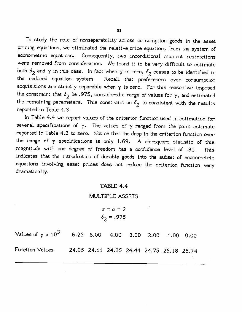
To study the role of nonseparability across consumption goods in the assetpricing equations, we eliminated the relative price equations from the system ofeconometric equations. Consequently, two unconditional moment restrictionswere removed from consideration. We found it to be very difficult to estimateboth and y in this case. In fact when y is zero, ceases to be identified inthe reduced equation system. Recall that preferences over consumptionacquisitions are strictly separable when y is zero. For this reason we imposedthe constraint that be .975, considered a range of values For y, and estimatedthe remaining parameters. This constraint on is consistent with the resultsreported in Table 4.3.
In Table 4.4 we report values of the criterion function used in estimation forseveral specifications of y. The values of y ranged from the point estimatereported in Table 4.3 to zero. Notice that the drop in the criterion function overthe range of y specifications is only 1.69. A chi-square statistic of thismagnitude with one degree of freedom has a confidence level of .81. Thisindicates that the introduction of durable goods into the subset of econometricequations involving asset prices does not reduce the criterion function verydramatically.
TABLE 4.4
MULTIPLE ASSETS
oa=262 .975
Values of y x 6.25 5.00 4.00 3.00 2.00 1.00 0.00
Function Values 24.05 24.11 24.25 24.44 24.75 25.18 25.74

32
Finally, we report evidence regarding the restrictions on the growth rates ofquantities and prices. Recall that the first block of six unconditional momentrestrictions depends only on the five parameters pi, p2, 1 - '2 and the•two parameters of 4,. Consequently, these five parameters can be estimatedseparately. Furthermore, these six moment restrictions are the source of oneof the over-identifying restrictions that were tested using the test statistic.It is of interest to examine these six moment conditions in isolation.
In Table 4.5 we report the constrained estimates of p1, 2 and i_P2.using only these six orthogonality restrictions. In addition, we report theunconstrained estimates obtained by relaxing the restriction that the growth ratein relative prices equals p1-p2. The T statistic provides some evidenceagainst the restrictions on the growth rates, but the evidence is not overwhelm-ing. This is consistent with the results reported In Table 4.2 indicating thatthere is more evidence against the over—identifying restrictions when trendestimation is taken into account.6
TABLE 4.5INFERENCE ON GROWTh RATES
Pararn eters* Constrained Unconstrained
p1 x 1O 2.80 2.92(.05) (.08)
X 10 4.37 4.87(.09) (.25)
(p1 - p2) x IO -1.57 -1.45(.07) (.09)
** 4.43
(.965)
*standard errors are in parentheses.**probability values of test statistics are in parentheses.

33
Summarizing the results in this section, we found a high degree ofsubstitutability between nondurable goods and the services from the stock ofdurable goods. Also, we found that goods which are classified as nondurablegenerate service flows which extend beyond the purchase date in monthly data.On the other hand, we found very little evidence in support of adjustment costs ineither the stock of durable goods or in nondurable goods. All of these resultswere obtained under the maintained assumption that the preferences ofconsumers are quadratic. In the next section we investigate these empiricalhypotheses using other specifications of preferences.

34
V. S BRANCH PREFERENCES
In this section we consider results obtained when a is estimated althoughconstrained to be less than one. The household technology is modified from thatused in section four by eliminating the fourth capital stock and the third serviceand setting the parameter y to zero. Hence n and m are both two. The matrices, e, and r are parameterized as
o o 0 [1 OJ 11 o(5.1) = c5 0 0 ê = 0 O
F =LO 0 1
o o 62 [Although y is zero, a is no longer required to be equal to a. Hence, in thisspecification, a dictates the substitutability between the services from durableand nondurable consumption goods. Finally, the economy-wide averagesubsistence point u is set to zero, and the preference parameters & and arenormalized so that their sum is one.
We report results pertaining to four hypotheses. The first hypothesis is
Under this hypothesis the function U used in representing preferences forconsumption services has the Cobb-Douglas form given by (1.3).
The second hypothesis is
H2:a1Under this hypothesis the services from durables and nondurables are perfectsubstitutes. This hypothesis is the analogue to the second hypothesis in sectionfour.
The third hypothesis is
H3 : a = a

35
Under this hypothesis the implied preferences for consumption goods arestrictly separable across durable and nondurable consumption goods. Thishypothesis is the analogue to the third hypothesis in section four and wasmaintained by Grossman and Shiller (1981) and Hansen and Singleton (1982,1983).
The fourth hypothesis is
H4:cra=OUnder this hypothesis preferences are logarithmically separable over the twoconsumption services as was assumed by Muellbauer (1981).
In our empirical analysis, we transformed the original econometric equationsas follows. We formed w1 +(t) =
w1 (t) /mu2 (t) and w2(t) = w2 (t) /rnu1 (t).Since mu (t) and mu2 Ct) are in 1(t), E [w1 (t) 11(t)] = 0 and E [w2 +(t) 11(t)] = 0.Hence the unconditional moment restriction
(5.2) E[z(t)w(t)j 0
is satisfied where z(t) is a matrix comfortable to w(t) with elements that arein 1(t) such that Iz(t)w(t)I has a finite expectation. This transformation ofequations accomplishes two things. First, each of the resulting equations has aconstant term that is normalized to unity. Second, the resulting econometricequations are expressed in terms of marginal rates of substitution forconsumption services rather than marginal utilities. This latter featureguarantees that our econometric equations can be expressed in terms of ratios ofconsumption services. This feature is particularly convenient for the specialcase in which a is zero (Cobb-Douglas) as we will see subsequently.
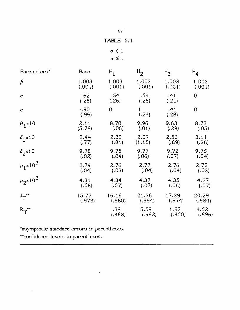
The model was estimated using the procedures described in section three andthe data described in section four. The results are presented in Table 5.1 asthe base run. The estimated standard errors of a and a are sufficiently largerelative to the respective point estimates to indicate that each of the hypotheses
H1, H2, and H4 may be empirically plausible. Also, the estimated standarderror of 01 is quite large relative to its point estimate. The estimate of the

36
parameter governing depreciation in nondurables (ó) is positive and largerelative to its standard error implying that nondurable consumption goodsgenerate consumption services in time periods subsequent to their acquisition.The point estimate of the parameter governing depreciation in durables (62) isthe same as was obtained when preferences were assumed to be quadratic (seeTable 4. 1). The estimate of the discount factor (IS) exceeds one reflecting thelow ex post returns to holding Treasury Bills during our sample period.Finally, the T statistic is somewhat lower than the corresponding statistic forthe base quadratic run.7 There is still, however, some evidence against the over-identifying restrictions.
37
TABLE 5.1
a�iParameters* Base H1 H2 H3 H4
1.003 1.003 1.003 1.003 1.003(.001) (.001) (.001) (.001) (.001)
a .62 .54 .54 .41 0(.28) (.26) (.28) (.21)
a -.90 0 1 .41 0(.96) (.24) (.28)
e xlO 2.11 8.70 9.96 9.63 8.731 (5.78) (.06) (.01) (.29) (.05)
6 xlO 2.44 2.30 2.07 2.56 3.111 (.77) (.81) (1.15) (.69) (.36)
6 xlO 9.78 9.75 9.77 9.72 9.752 (.02) (.04) (.06) (.07) (.04)
p x103 2.74 2.76 2.77 2.76 2.721 (.04) (.03) (.04) (.04) (.03)
p x103 4.31 4.34 4.37 4.35 4.272 (.08) (.07) (.07) (.06) (.07)
15.77 16.16 21.36 17.39 20.29(.973) (.960) (.994) (.974) (.984)
RT** .39 5.59 1.62 4.52(.468) (.982) (.800) (.896)
*asyptotic standard errors in parentheses.**co?idence levels in parentheses.

38
Table 5. 1 also reports our results from testing hypotheses H1 through H4.According to the reported RT statistics, there is very little evidence againsthypothesis H1 and only weak evidence against hypotheses H3 and H4. Of the fourhypotheses, H2 appears to be the least plausible empirically.
It is of interest to compare the results of the hypothesis tests reported inTables 5.1 to those in 4.1. Overall, there is somewhat less evidence againstthe over-identifying restrictions when cr is estimated (although constrained to beless than one) than when preferences are assumed to be quadratic (u=2). Also,there is more evidence against the perfect substitutability hypothesis (H2) andless evidence against the strict separability hypothesis (H3) -
All of the empirical results discussed so far correspond to the first of thetwo models of growth discussed in sections one and two. We now examine theempirical plausibility of these two models. In Table 5.2 we report resultsfrom estimating regressions of log[e1*(t)j, logfe2*(t)], and log{q2*(t)] onto aconstant, a time trend, and one lag of the respective variable. Under the firstmodel of growth, the coefficients on the lag of the variables should have absolutevalues that are less than one. The estimates of the asymptotic standard errorsthat are reported in the parentheses were calculated under the presumption thatthe First model of growth is the appropriate model. Under the second model ofgrowth, the coefficient on the time trend should be zero and the coefficient onthe lag of the variable should be one. Dickey and Fuller (198 i) deduced theasymptotic distribution of the likelihood ratio test when the disturbance termsin the regression are normal independent random variables and the second modelof economic growth is the appropriate model. Let .ZT denote the likelihood ratiotest statistic suggested by Dickey and Fuller (1981). Phillips and Peron (1985)showed how to modify the test statistic to accomodate more general distribu-tional assumptions while preserving the same asymptotic distribution that wastabulated by Dickey and Fuller (1981). In particular, Phillips and Peronallowed for more general forms of serial dependence and conditional heteroske-dasticity in the disturbance term. Let ZT* denote the modification of thelikelihood ratio statistic suggested by Phillips and Peron.8

39
TABLE 5.2TESTS FOR UNIT ROOTS
Right-hand-side variable Nondurables and Services Durables Relative Prices
Constant 0.15 0.13 0.004(0.04) (0.03) (0.004)
Time Trend x 10 1.26 4.32 -0.36(0.35) (1.08) (0.26)
Lag 0.96 0.91 0.98(0.01) (0.02) (0.02)
ZT 2.65 5.50 2.00
2.60 6.15 2.72
*asymptotic standard errors in parentheses
Dickey and Fuller (1981) reported critical values for their test statistic ofabout 5.4 for confidence level .9 and 6.3 for confidence level .95. Hence thetime series on durable goods is the only one for which there is much evidenceagainst the second model of growth. Even for this series, the evidence is notoverwhelming. Dickey and Fuller also indicated that the likelihood ratio testdoes not have very much power against many alternatives that are special cases
of our first model of growth. Consequently, the results in Table 5.2 indicate
that it is very difficult to discriminate between the two models of growth
suggested in section one using the data set we considered. For this reason, wealso report results for the second model of growth. A cost of using this modelis that our statistical methods are applicable only under hypothesis (a0).

40
To estimate the parameters under H1 and the second model of growth, wechose the matrix z(t) to be
e *(t)/e *(t- 1)
Ii 0e2*(t)/e2*(t1)
(5.3) Z(t) =La 1
q2*(t)e2*(t)/ej*(t)
y(t)I
Thus, we imposed ten unconditional moment restrictions to estimate the fiveparameters , a, 01 c, and 62. Our estimation results are reported in Table5.3 under the column heading Single Asset. The estimation equations for theasset return and the relative price are identical with those used to obtain theresults in Table 5.1 under the column H1. Not suprisingly, the point estimatesreported in these two columns are very similar. There is some difference in theestimated standard errors because of differences in the estimation equations forthe growth parameters and in the choice of the matrix z (t). For instance, theestimate of o in Table 5.3 is again about .5 although the estimated standarderror is larger than in Table 5.1. The estimate of in Table 5.3 is againpositive but is estimated with less precision than In Table 5.1. The estimatesof and 62 are very close to those reported in Table 5.1, but the correspondingestimated standard errors are smaller.
Table 5.3 also reports results from estimating the model when two assetpricing equations were considered simultaneously. Let y1 (t+1) and y2(t+1)denote the ex post returns on one-month Treasury Bills and a value-weightedindex of stocks on the New York Stock Exchange. The matrix z (t) was chosen tobe
ej*(t)/ej*(t_1)100 y(t)(5.4) z(t) = 0 1 0 0
y2(t)001I

41
TABLE 5.3
cT<ia0
Preferences* Single Asset Multiple Assets
.999 1.005(.004) (.003)
-.51 -.36(.61) (.55)
91x10 8.63 8.62(.02) (.03)
ó1xiO 3.06 3.80(1.59) (.55)
62x10 9.70 9.71(.05) (.030)
p1x103 2.95 2.99(.22) (.19)
p2x103 5.55 4.671.19 (1.23)
8.35 19.14(.862) (.992)
*standard errors in parentheses.**pbability values of test statistic.
Thus we imposed twelve unconditional moment restrictions. The results arereported under the column Multiple Assets.

42
The point estimates in this case are very similar to those obtained using onlyone asset return. As in Hansen and Singleton (1982), however, there issubstantially more evidence against the model when two asset returns are used.This is not surprising because we found very little evidence against thehypothesis that preferences are logarithmically separable.

43
CONCLUSIONS
In this paper we presented a set of empirical results pertaining to inter- andintraternporal substitutability of consumption goods. The results in section fourindicate that when preferences are constrained to be quadratic, there is verylittle evidence against the hypothesis that the services from durable goods andnondurable goods are perfect substitutes. This finding supports the practice ofaggregating these services into a single service. On the other hand, this findingis inconsistent with the existence of constant real interest rates because pricesof durable goods relative to nondurable goods are not constant over time. Inaddition, these results call into question the practice of testing quadratic modelsof aggregate consumption using data on nondurables and services only.
The finding of perfect substitutability between service flows of thesedifferent consumption goods is admittedly extreme and possibly sensitive to thespecification of preferences. For this reason, we reported results using Sbranch preference specifications. The results in section five show that for Sbranch prefence specifications, there is more evidence against perfectsubstitutability between service flows, but less evidence against strictseparability across durable and nondurable consumption goods. Among otherthings, these findings suggest that the empirical shortcomings of theintertemporal asset pricing model cannot be attributed to the neglect of durablegoods.
For both specifications of preferences, we found that goods classified asnondurable goods generate positive consumption services in subsequent timeperiods. Since this finding may be sensitive to aggregation-over--time biases, itwould be of interest to examine this hypothesis using a model in whichconsumers make decisions more frequently than once a month and theconsumption data are viewed as monthly averages over finer intervals of time.
The models we considered in this paper are important benchmarks formodels with endogenous depreciation, private information, and/or lumpiness inthe acquisition of durable goods. Deducing testable implications from modelswith these alternative features will be a challenging but possibly fruitful task.We hope that by documenting the empirical shortcomings of the benchmarkmodels, we have made this task a little easier.

44
NOTES
1For our analysis, it is convenient to view economies with capital accumulationas being in a suitably defined stochastic steady state. Alternatively, one coulduse a model for which suitably transformed values of consumption and capitalgoods converge to a stochastic steady state starting from arbitrary initialconditions. Often, the rate or convergence to the stochastic steady state issufficiently fast so that the initial conditions do not effect the asymptoticdistribution of the econometric estimators.
Follows from the analysis in Hansen (1987) where it is shown that thereare multiple ways to represent quadratic preferences when there are moreservices than goods. In particular, it is shown that the preferences can alwaysbe represented equivalently with the same number of services as goods but witha different Corrnan-Lancaster technology.
3The use of seasonally adjusted data is potentially problematic since ourtheoretical model provides no rationale for such adjustments. Miron (1986) hasstudied the impact of seasonal adjustment of consumption in models similar tothose considered here.
4me results reported in all tables except 5.2, used a value of = 15 to estimate2. Also, we continued using previous round parameter estimates p to obtain eeeew estimates of 2 until the probability value of statistic did not change inthe third decimal place.
5The examination of the timing convention is not a substitute for investigatingthe effects of aggregation-over-time-biases that might occur. For instance,aggregation-over-time-biases can occur if consumers make consumption decisionscontinuously and an econornetrician's time series data is the total consumptionover an interval of time. Such biases can easily distort estimates ofintertemporal substitution parameters such as c5. In this paper we maintain theassumption that consumption decisions are made monthly.

45
6Bernanke (1985) studied the behavior of consumption of nondurabies andservices and durables by assuming that the growth rate in both series were thesame as the growth rate in GNP. His assumption is clearly incompatible withthe results in Table 4.5.
7The minimized values of the criterion functions reported in Tables 4.1 and 5. 1are not directly comparable because the form of the estimation equations isdifferent and because the restrictions on preferences across these two tables arenot nested. In principle, one could estimate a preference specification forconsumption services that nests both of the preference specifications used inTables 4.1 arid 5.1. Such a nesting is given in section one. Most likely, theresulting criterion function used in such an estimation would not be very wellbehaved. The results in both Tables 4.1 and 5.1 confirm that unless additionalrestrictions are imposed, it is difficult to estimate all of the preferenceparameters. Non-nested testing procedures such as those suggested by Cox(1961) require that more structure be imposed on the estimation problem thanwe have imposed here.
implement the ?hlllips-?eron test, one must estimate a limit like that givenon the right-hand side of (3.14). We found some sensitivity of the estimatedstandard errors and the statistic to the choice of 9, although this sensitivitywas never sufficient to reverse conclusions. The results reported in Table 5.2take I to be 20.

46
APPENDIX A
In this appendix we present specifications of preferences and servicestechnologies that are consistent with our modeling of growth in prices andquantities.
Consider first the service technology. Let k*j (t) denote the vector of unscaled
household capital stocks of person j, and c (t) denote the vector of unscaled new
consumption goods of person j. The unscaled counterpart to (1.4) is
(A. 1) k*J(t) = *k*J(t_1) + e*(t)c*J(t)
where * = exp(p5)L and e*(t) = exp(p5t)eA(t11. We use (1.5) to map thehousehold capital stock into consumption services. The matrix Function e*(t)governs the technological progress in this mapping. Equation (A.1) is designedso that
(A.2) r(t) = Fg*(t) =exp(p5t)f(t)
where {f*(t) : t�1} and {g*(t) : are the economy-wide unscaled averageprocesses on consumption services and household capital. Hence an implicationof this technology in conjunction with our assumption about the growth inequilibrium acquisitions of new consumption goods is that the equilibriumgrowth rate in consumption services is for all services.
Next, we consider specifications of preferences. When equilibriumconsumption grows over time and c is greater than one, it is necessary for thepreference shocks to grow over time to avoid the implication that consumersbecome satiated. Similarly, when o is less than one, it is necessary forpreference shocks to grow in order for the impact of the subsistence levels notto diminish over time. Thus, to allow for growth in services we transform thepreference shock processes for each individual. Let uJ*(t) u (t)exp(tu5), sothat the growth rate in the preference shocks is the same as the growth rate inthe equilibrium consumption service vector. Also, define exp(-p5cñ8. Then
the preferences over unscaled consumption services are given by (1.1) and (1.2)with sJ*(t), uJ*(t), and * replacing s3(t), u(t), and respectively.

47
It is easy to verify that this specification of preferences and servicetechnology rationalizes our treatment of growth in prices and new consumptiongoods. Notice that there is a restriction linking the growth rates in equilibriumaggregate consumption and technological progress in the Corman-Lancastertechnology. This restriction is not deduced from more primitive assumptionsbut is simply posited. On the other hand, this restriction has empirical contentand can be tested.
The growth rate and the discount factor * are left unidentified in ouranalysis because direct observations are not available for consumption services.These parameters must satisfy particular inequality restrictions, however. Forinstance, is less than one, and
(A.3) j.> log()/o for ci'> 0
(A.4) ji5 <log()/a for ci <0

REFERENCES
Bernanke, B.S., uAdjustrnent Costs, Durables, and Aggregate Consumption,"Journal of Monetary Economics, Vol 15 (1985) 4 1-68.
Boyce, R., "Estimation of Dynamic Gorman Polar Form Utility Functions,"Annals of Economic and Social Measurement, 4:1 (1975), 103-116.
Brown., M.J., and 0. Helen, "The S-Branch Utility Tree: A Generalization ofthe Linear Expenditure System," Econometrica, 40 (1972) 737-747.
Cox, D.R., "Tests of Separate Families of Hypotheses," Proceedings of theFourth Berkeley Symposium in Mathematical Statistics and Probability,University of California Press (1961) 105-123.
Darby, M.R., "Post War US Consumption, Consumer Expenditures, andSavings," American Economic Review, Papers and Proceedings, 65(1975) 217-222.
Dickey, D.A. and W.A. Fuller, "Distribution of the Estimators forAutoregressive Time Series with a Unit Root," Econornetrica, 49,(1981) 1057-1072.
Eichenbaum, M.S, L.P. Hansen, and S.F. Richard, "The Dynamic
Equilibrium Pricing of Durable Consumption Goods," manuscript (1984).
Flavin, M.A., "The Adjustment of Consumption to Changing ExpectationsAbout Future Income," Journal of Political Economy, 89 (1981) 974-1009
Gallant, A.R., and D.W. Jorgenson, "Statistical Inference for a System ofSimultaneous, Nonlinear, Implicit Equations in the Context ofInstrumental Variable Estimation," Journal of Econometrics 11 (1979)275-302.
Gorman, W.M., "Community Preference Fields," Econometrica (1953) 63-80.
Gorman, W.M., "A Possible Procedure for Analyzing Quality Differentials inthe Egg Market," Review of Economic Studies 47 (1980) 843-856.
1

Granger, C.W.J., "Some Properties of Time Series Data and Their Use inEconometric Model Specification," Journal of Econometrics, (1981) 121 -130.
Grossman, S.J., and R.J. Shiller, "The Determinants of the Variability ofStock Market Prices," American Economic Review 71 (1981) 222-227.
Hall, R.E., "Stochastic Implications of the Life Cycle-Permanent IncomeHypothesis: Theory and Evidence," Journal of Political Economy 86(1978) 971-987.
Hansen, L.P., "Large Sample Properties of Generalized Method of MomentsEstimators," Econometrica 50 (1982) 1029-1054.
_________—, "Lecture Notes on Time Series Econometrics," manuscript(1986).
___________ "Calculating Asset Prices in Three Example Economies,"(forthcoming in Ed. T.F. Bewley, Advances in Econometrics, Fifth World
Congress, 1987).
___________ and S.F. Richard, "The Role of Conditioning Information inDeducing Testable Restrictions Implied by Dynamic Asset PricingModels," (forthcoming in Econometrica, 1987).
__________ and K.J. Singleton, "Generalized Instrumental VariablesEstimation of Nonlinear Rational Models," Econometrica 50 (1982)1269-1286.
_________________________________ "Stochastic Consumption, Risk Aversion,and the Temporal Behavior of Asset Returns," Journal of PoliticalEconomy 91:1 (1983) 249-265.
Houthakker, H.S. and L.D. Taylor, Consumer Demand in the United States1929-1970, 2nd Edition, Harvard University Press, Cambridge, MA(1970).
Ibbotson, R.G., and R.A. Sinquefeld, Stocks, Bonds, Bills, and Inflation:
Historical Returns, 1926-1978, 2nd. ed. Charlottesville, VA: Financial
Analysts Res. Found. (1979).
2

Kydland, F.E., and E.F. Prescott, "Time to Build and AggregateFluctuations," Econometrica 50 (November 1982) 1345-1370.
Lancaster, K., "A New Approach to Consumer Theory," Journal of Political.Economy 74 (1966) 132-157.
Mankiw, N.G., "Hall's Consumption Hypothesis and Durable Goods," Journalof Monetary Economics 10 (1982) 417-425.
Miron, Jeffrey A., "Seasonal Fluctuations and the Life Cycle-PermanentIncome Model of Consumption," J.P.E., 94:6 (1986) 1258-79.
Muellbauer, J., "Testing Neoclassical Models of the Demand for ConsumerDurables," Theory and Measurement of Consumer Behavior, A. Deatori(ed.), New York: Cambridge University Press (198 1).
Musgrave, J.C., "Durable Goods Owned by Consumers in the United States,1925-1977," Survey of Current Business (March 1979).
Newey, W., and K.D. West, "A Simple, Positive Definite, Heteroskedasticityand Autocorre lation Covariance Matrix," (forthcoming in Econometrica1987).
Novales., A., "A Stochastic, Monetary Equilibrium Model of the InterestRate," manuscript, SUNY at Stony Brook (1985).
Peck, S.C., "The Individual's Choice of Goods, Assets and Durables," SecondWorld Congress of the Econometric Society paper (1970).
Phillips, P.C.B. and P. Perron, "Testing for a Unit Root in Time SeriesRegression," mimeo (1986).
Pollak, RA., "Habit Formation and Dynamic Demand Functions," Journal ofPolitical Economy, 78, (1970) pp. 745-763.
Sargent, T.J., "Rational Expectations, Econometric Exogeneity, andConsumption," Journal of Political Economy 86:4 (1978) 673-700.
Sims, C.A., "International Evidence on Monetary Factors in MacroeconomicFluctuations," manuscript (1.980).
Telser, L.G., and R.J. Graves, Functional Analysis in MathematicalEconomics. Chicago: University of Chicago Press (1972).
3