Estimating Inter Regional Trade Patterns

8/8/2019 Estimating Inter Regional Trade Patterns

http://slidepdf.com/reader/full/estimating-inter-regional-trade-patterns 1/49

1

A Flexible Modeling Framework to Estimate Interregional

Trade Patterns and Input-Output Accounts

Patrick Canning, Economic Research Service, US Department of AgricultureZhi Wang, School of Computational Sciences, George Mason University

(First Draft-Do not quote)

Abstract

This study implements and tests a mathematical programming model to estimate

interregional, interindustry transaction flows in a national system of economic regions based on

an interregional accounting framework and initial information of interregional shipments. A

complete national IO table, regional sectoral data on gross output, value-added, exports, imports

and final demand are used as inputs to generate an interregional input-output system that

reconciles regional market data and interregional transactions. The analytical and empirical

properties of the model are discussed in detail. The model is tested by a 3-region 10-sector

example against data aggregated from the version 4 GTAP database. It shows that the model has

remarkable capacity to discover the true interregional trade pattern from highly distorted initial

estimates. The paper also discusses an application of the model to estimate an interregionalinput-output account for the US economy based on the BEA 1997 national benchmark IO table

and detailed state level data from the 1997 economic Census and other sources.

April 30, 2003

Paper prepared for presentation at the Sixth Annual Conference on Global Economic Analysis,June 12-14, Scheveningen, The Netherlands.



2

I. Introduction

A major obstacle in regional economic analysis is the lack of consistent, reliable regional

data, especially data on interregional trade and inter-industrial transactions. Despite decades of

efforts by regional economists, data analogous to national input-output accounts and

international trade accounts, which have become increasingly available to the public today, still

are generally not available even for well defined sub-national regions in many developed

countries. Therefore, regional economists have had to develop various non-survey methods to

estimate such data.

This paper present a flexible modeling framework to estimate interregional trade flows

and input–output accounts for a national system of economic regions. The approach employed

simultaneously optimizes the information gained by data available from different sources in a

consistent interregional accounting system. Typically, data from different statistical sources have

substantial gaps and inconstancies that preclude routine solutions from being obtained without

modification. Our approach allows all relevant information to be incorporated in the data

adjustment process in an internally consistent manner with an objective ranking of their relative

reliabilities, and is also flexible enough in the model specification to use useful information from

all possible sources. While the applications of this modeling framework may be quite broad, its

design has been specifically targeted to the problem of developing spatial enhancements to a

national input-output account for economies with well-defined economic sub-regions.

This paper is organized as follows. Section II specifies the modeling framework and

discusses its theoretical and empirical properties. Section III tests the model by using a 3- region,

10-sector data set aggregated from the version 4 GTAP database. Test results from seven

experiments were evaluated against eight Mean Absolute Percentage Error indexes. Section IV



3

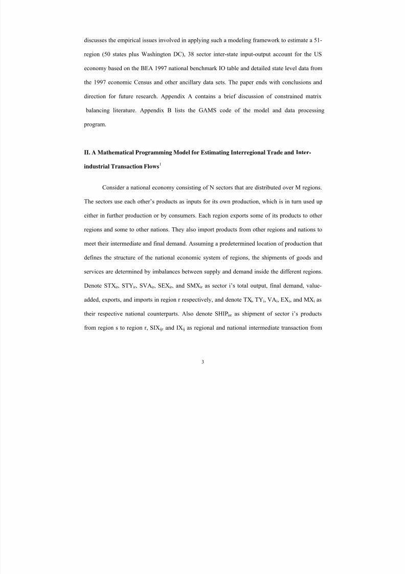
discusses the empirical issues involved in applying such a modeling framework to estimate a 51-

region (50 states plus Washington DC), 38 sector inter-state input-output account for the US

economy based on the BEA 1997 national benchmark IO table and detailed state level data from

the 1997 economic Census and other ancillary data sets. The paper ends with conclusions and

direction for future research. Appendix A contains a brief discussion of constrained matrix

balancing literature. Appendix B lists the GAMS code of the model and data processing

program.

II. A Mathematical Programming Model for Estimating Interregional Trade and Inter-

industrial Transaction Flows1

Consider a national economy consisting of N sectors that are distributed over M regions.

The sectors use each other’s products as inputs for its own production, which is in turn used up

either in further production or by consumers. Each region exports some of its products to other

regions and some to other nations. They also import products from other regions and nations to

meet their intermediate and final demand. Assuming a predetermined location of production that

defines the structure of the national economic system of regions, the shipments of goods and

services are determined by imbalances between supply and demand inside the different regions.

Denote STXir , STYir , SVAir , SEXir , and SMXir as sector i’s total output, final demand, value-

added, exports, and imports in region r respectively, and denote TXi, TYi, VAi, EXi, and MXi as

their respective national counterparts. Also denote SHIPisr as shipment of sector i’s products

from region s to region r, SIXijr and IXij as regional and national intermediate transaction from



sector i to sector j respectively. All variables are measured in annual values. In such a static

national system of economic regions, the following accounting identities must hold at each given

year for all i ∈ N and s, r ∈ M.

STX =SVASIX ir ir jir

n

j=1

+∑ (1)

SMX SHIP=STY SIX ir isr

m

=1s

ir ijr

n

j=1

++ ∑∑ (2)

(3) STX =SEX SHIP ir ir irs

m

=1s

+∑

(4) IX SIX ijijr

m

=1r

= ∑

(5) TX STX iir

m

=1r

= ∑

VASVA iir

m

=1r

= ∑ (6)

TY STY iir

m

=1r

=

∑(7)

EX SEX iir

m

=1r

= ∑ (8)

MX SMX iir

m

=1r

= ∑ (9)

The economic meanings of each of the nine equations are straightforward: equation (1)

defines the sum of sector i’s intermediate and primary factor inputs equals the sector’s total

output in each region. Equation (2) states the sum of each region’s intermediate and final demand

4

1 The modeling framework is also a special case of constrained matrix balancing problem frommathematical perspective. It is a core mathematical structure for diverse empirical applications. See



must be met by shipments from all regions (including from its own) within the nation plus

imports from other nations. Equation 3 defines a region can only ship to all regions within the

nation and export to other nations what it produces2,

while equations (4) –(9) are simply the facts

that sums of all the region’s economic activities within a nation must equal to the national totals.

Having those accounting identities in mind, the estimation problem can be formally stated as

follows:

Given a n × m × m non-negative array SHIP0

= {ship0

isr } and a n × n × m non-negative array

SIX 0

= {six0ijr }, determine a non-negative array SHIP = {shipisr } and a non-negative array SIX =

{sixijr } that is close to SHIP0

and SIX 0

such that equations (1) to (9) are satisfied, where s ∈ M

denotes the shipping regions, r ∈ M denotes the receiving regions, and i, j ∈ N denotes the make

and use sectors respectively.

In plain English, the estimation problem is to modify a given set of prior inter-regional and inter-

industrial transaction estimates to satisfy the above nine known accounting constraints. The

mathematical programming model conducting the estimation uses an objective function that

penalizes the deviations of the estimated array SHIP and SIX from the initial array SHIP0

and

SIX0. Two types of alternative functional forms could be used:

(i) Quadratic function:

}{0

11

Minijr

2

ijr ijr m

=1r

n

j=1

n

iisr

20

isr isr m

=1r

m

=1s

n

i wi

)six-(SIX +

sw

)ship-SHIP(

2

1 = Z ∑∑∑∑∑∑

==

(10)

(ii) Entropy function:

) /six LN(SIX wi

SIX +) /ship LN(SHIP

sw

SHIP = Z ijr ijr

isr

isr m

r

n

j=1

n

=1i

irsirs

isr

isr m

r

m

=1s

n

=1i

0

1

0

1

Min •• ∑∑∑∑∑∑==

(11)

There are desirable theoretical properties of the above estimation framework that are well

documented in the literature. Firstly, it is a separable nonlinear programming problem subject to

appendix A for details.

5



linear constraints. The entropy function is motivated from information theory and is the objective

function underlying the well-known RAS procedure with row and column totals known with

certainty (Senesen and Bates, 1988). It measures the information surprise contained in SHIP and

SIX given the initial estimates ship0 and six0. The quadratic penalty function is motivated by

statistical arguments. There are different statistical interpretations underlying the model by

choices of different reliability weights swisr and wiijr . When the weights are all equal to one,

solution of this model gives a constrained least square estimator. When the initial estimates are

taken as the weights, solution of the model gives a weighted constrained least square estimator,

which is identical to the Friedlander-solution, and a good approximation of the RAS solution.

When those weights are proportional to the variances of the initial estimates and the initial

estimates are statistically independent (the variance and covariance matrix of ship0

and six

0are

diagonal), the solution of the model yields best linear unbiased estimates of the true unknown

matrix (Byron, 1978), which is identical to the Generalized Least Squares estimator if the

weights equal to the variance of initial estimates (Stone, 1984, Ploeg, 1984). Furthermore, as

noted by Stone et al. (1942) and proven by Weale (1985), in cases where the error distributions

of the initial estimates are normal, the solution also satisfies the maximum likelihood criteria.

The corresponding likelihood function can be written as:

exp}{

00

2wi

)six-SIXi( +

2ws

)ship-SHIP( -

2

mmn

ijr 2

mmn -

isr

n

j=1

m

=1i

ijr

2ijr jr

isr

2isr isr

))= L wi(2ws(2 •••••

∏∏ π π (12)

6

2 Put another way, SHIPisr describes the process of transforming sector output i of region s into either aninput of any sector j or the property of any final user in region r.



Secondly, the quadratic and entropy objective functions are equivalent in the

neighborhood of initial estimates, under a properly selected weighing scheme. By taking second

order Taylor expansion of the likelihood function (12) at point (shipisr , sixijr ) we have

R+

six2

)SIX -(

+ +ship2

)SHIP-ship( +-SHIP= Z

ijr

2

ijr ijr m

=1r

n

j=1

n

i0

isr

20

isr isr m

=1r

m

=1s

n

j

0ijr

2

ijr ijr

ijr ijr

m

=1i0isr

2isr

0isr

isr isr

m

r

m

=1s

n

i=i

six

)six-(SIX +

ship

)ship-SHIP(

2

1

sixsixSIX ship

}{0

0

11

0

00

1

}{}{

∑∑∑∑∑∑

∑∑∑∑

==

=

=

−

(13)

This is the quadratic function (10) plus a remainder term R. As long as the posterior estimates

and the prior estimates are close and the prior estimates are used as reliability weights3, the term

R will be very small and the two objective functions thus can be regarded as approximating one

another.

Thirdly, as proved by Harrigan (1990), in all but the trivial case, posterior estimates

derived from entropy or quadratic loss minimand will always better approximate the unknown,

true values than do the associated initial estimates. In this framework, information gain is

interpreted as the imposition of additional valid constraints or the narrowing of bounds on

existing constraints as long as the true but unknown values belong to the feasible solution set.

This is because adding valid constraints or further restricting the feasible set through the

narrowing of interval constraints cannot move the posterior estimates away from the true values,

unless the additional constraints are non-binding (have no information value). Although the

7

3 The quadratic functional form has a numerical advantage in implementing the model. It is easier tosolve than the entropy function in very large models because they can be solved by software specificallydesigned for quadratic programming.



8

posterior estimates may not always be regarded as providing a "reasonable" approximation to the

true value4, the resulting constrained estimates are always better than the initial estimates in the

sense the former is closer to the true value than the later, so long as the imposed constraints are

true. In other words, the optimization process has the effect of reducing, or at least not

increasing, the variance of the estimates. This property is simple to show by using matrix

notation. Define W as the variance matrix of initial estimates ship0, A as the coefficient matrix of

all linear constraints. The least squares solution (equivalent to the quadratic minimand as noted

above) to the problem of adjusting ship0 to SHIP, which satisfies the linear constraint, A•SHIP =

0 can be written as:

SHIP = (I - WAT(AWA

T)-1

A)SHIP0

(14)

Thus var(SHIP) = (I - WAT(AWAT)-1A)W = W - WAT(AWAT)-1A)W (15)

since WAT(AWA

T)

-1A)W is a positive semi-definite matrix, the variance of posterior estimates

will always be less, or at least not greater than the variance of the initial estimates as long as

A•SHIPtrue = 0 holds. This is the fundamental reason why such an estimating framework will

provide better posterior estimates. Imposing accounting relationship’s (1)–(9) will definitely

improve, or at least not worsen the initial estimates, since we are sure from economics those

constraints are identities and must be true for any national system of economic regions.

Finally, the choice of weights in the objective function has very important impacts on the

estimation results. For instance, using the initial estimates as weights has the nice property that

each entry of the array is adjusted in proportion to its magnitude in order to satisfy the

4The minimand objective function reflects the principle that the 'distance' between the posterior and prior

estimates should be minimized. While what we would like is to minimize is the 'distance' between the posterior estimates and the unknown true values. This 'distance' can not be measured, but a goodestimation procedure should have a desirable influence on it.



accounting identities, and the variables can not change sign and that large variables are adjusted

more than small variables. However, the adjustment relates directly to the size of the initial

estimates ship0

isr and six0

ijr, and does not force the unreliable prior to absorb the bulk of the

required adjustment. Furthermore, only under the assumptions: (1) the initial estimates for

different elements in the array are statistically independent, and (2) each error variance is

proportional to the corresponding initial estimates, this commonly used weighing scheme

(underlying RAS) can obtain best unbiased estimates, while those assumptions may not hold in

many cases. Fortunately, the model is not restricted to use a diagonal-weighing matrix such as

the priors only. When a variance-covariance matrix of the initial estimates is available, it can be

incorporate into the model by modifying the objective function as follows:

)SIX -SIX (WI )SIX -(SIX +)SHIP-SHIP(WS)SHIP-SHIP(= Z -1T -1 0000Min (16)

The efficiency of the resulting posterior estimator will be further improved if the error structure

of the priors is available, because such a weighting scheme makes the adjustment independent of

the size of the priors. The larger the variance, the smaller its contribution to the objective

function, and hence the less punishment for shipisr and sixijr to move away from their priors (only

the relative, not the absolute size of the variance affects the solution). A small variance of the

priors indicates they are very reliable data and thus should not change by much, whilst a large

variance of the priors indicates unreliable data and will be adjusted considerably in the solution

process. Therefore, this weighing scheme gives the best-unbiased estimates of the true, unknown

inter-regional and inter-industrial transaction value under the assumption that initial estimates for

different elements in the array are statistically independent. Although there is not much difficulty

to solve such a nonlinear programming problem like this today, the major problem is lack of data

to estimate the variance-covariance matrix associate with the priors.

9



10

Stone (1982) proposed to estimate the variance of six0ijr as var(six0

ijr ) = (θijr six0ijr )

2, where

θij is a subjectively determined reliability rating, expressing the percentage ratio of the standard

error to six0ijr . Weale (1989) had used time series information on accounting discrepancies to

infer data reliability. The similar methods can be used to derive variances associated with those

initial estimates in our model.

Despite the difficulties in obtaining data for the best weighting scheme, advantages of

such a model in estimating inter-regional shipments and inter-industrial transactions are still

obvious from an empirical perspective. Firstly, it is very flexible regarding the required know

information. For example, it allows for the possibility that the state total of output, value-added,

exports, imports and final demands are not known with certainty. In the real world, these

regional totals typically have substantial gaps and inconstancies with the national total.

Incorporating associated terms similar to SHIP0 and SIX0 in the objective function to penalize

solution deviations from the initial estimates from statistical sources allows the estimation of

those regional totals, together with entries in the inter-regional shipping and inter-industrial

transaction array. With the use of upper and lower bounds, this fact can also be modeled by

specifying ranges rather than precise values for the linear constraints (1) - (3). In addition, the

estimation of SHIP or SIX will be a special case of the framework when only one set of

additional data is available.

Secondly, it permits a wider variety and volume of information to be brought to bear on

the estimation process than what is possible with scaling methods. For example, the ability of

introducing upper and/or lower bounds on those regional totals is one of the flexibilities not

offered by commonly used scaling procedures such as RAS. The gradient of the entropy function

tends to infinity as shipisr and sixijr → 0, and hence restricts the value of the posterior estimates to



11

nonnegative. This is a desirable property of estimating inter-regional trade data. Such non-

negativity requirements can be enforced in the case of quadratic penalties through the use of

lower bounds on the values of shipisr and sixijr .

Thirdly, the weights in the objective function reflect the relative reliability of a given set

of priors. The interpretation of the reliability weights is straightforward. Entries with higher

reliability should be changed less than entries with a lower reliability. The choice of those

weights is also very flexible. They will use the best available information to insure that reliable

data in the prior estimates are not being modified by the optimization model as much as

unreliable data. In practice, such reliability weights can be put into a second array that has the

same dimension and structure as the priors. The inverted variance-covariance matrix of the priors

can be interpreted as the best index of the reliability for the initial data by statistics.

Finally, solution of this estimation problem exactly provide the data needed to construct a

so called multi-regional input-output (MRIO) model in the IO literature (Miller and Blair, 1985,

Isard, et al. 1998), which was pioneered by professor Polenske and her associates at MIT in the

1970’s (Polenske, 1980), and is still widely used in regional economic impact analysis today.

The above model could be easily extended to further allocate SIX and SHIP to

distinguish intermediate and final delivery of good and services within a national system of

economic regions. The extended model will be similar in many aspects with the interregional

accounting framework proposed by David F. Batten (1982) two decades ago. However, as we

will show later in this paper, it becomes more operational and provides much better empirical

estimation results on interregional shipments because of the explicit incorporation of

interregional trade flow information into both the initial estimates and the accounting framework.



To demonstrate, denote SXijsr as intermediate inputs delivered from sector i in region s to

sector j in region r within a nation, and SYihsr as final goods and services delivered from sector i

in region s to type h final demand in region r. Further, denote SIM ijr and SIYihr as imported (from

other nations) intermediate and final goods and services delivered to sector j or final demand

type h in region r respectively. Other notation regarding state total output, intermediate inputs,

value-added, exports and imports are the same with the aggregated model. Then the accounting

framework for the national system of economic regions can be defined as follows:

(17)STX =SVASIM SX ir ir

n

j

jir

m

s

jisr

n

j=1

+∑∑∑== 11

SMX STX =SEX SIY SY SIM SX ir ir ir

n

j

ihr ihrs

m

s

h

=1h

n

j

ijr ijrs

m

s

n

j=1

++++ ∑∑∑∑∑∑====

+

1111

(18)

STY SIY SY ir ihr

h

=1h

ihsr

m

=1s

h

=1h

= ∑∑∑ + (19)

SHIP=SY SX isr

h

h

ihsr

n

j

ijsr ∑∑==

+

11

(20)

SIX =SX ijr ijsr

m

s

∑=1

(21)

SMX =SIY SIM ir ir

n

j

ijr +∑=1

(22)

Adding a quadratic penalty objective function, we have an extended model to estimate a detailed

interregional input-output account based on the results from the earlier model5.

12

5 By incorporated the 6 accounting identities that the sum of all regions in the nation should equals their nationaltotals defined in equation (4-9), the model could be solved independently without use of the earlier model, however,the dimension of the model will be much higher and data requirements will be much larger than the earlier model.



}

{

0

1 1

0

1

0

11

0

1

Min

ihr

2

ihr ihr n

i

h

h

m

=1nijr

2

ijr ijr n

j=1

n

=1i

m

r

ihjr

2

ihsr ihsr n

j

h

h

n

i

m

=1nijsr

2

ijsr ijsr n

j=1

n

=1i

m

r

m

1s

wiy

)siy-SIY (

+wix

)sim-SIM (

wy

)sy-SY ( +

wx

)sx-SX (

2

1 = Z

∑∑∑∑∑∑

∑∑∑∑∑∑∑∑

= ==

====

+

(23)

This model has the theoretical and empirical properties similar to the earlier model, but

with much higher details. The solution to 23, subject to constraints 17-22, provides a complete

set of data for a so called inter-regional input-output (IRIO) model with imports endogenous in

the IO literature (Miller and Blair, 1985, Isard, et al. 1998).

III. Empirical Test of the Model and Evaluation Measures

3.1 The testing data set

How does the model specified above perform when applied to data from the real world?

In order to evaluate the models’ performance, a benchmark data set from the real world is

needed. Because good interregional trade data is quite rare and very difficulty to obtain in any

countries of the world, a natural place to find such data sets is existing global production and

trade databases such as the GTAP (Global Trade Analysis Project) database. For instance,

version 4 GTAP database contains detailed bilateral trade, transportation, and individual

country’s input-output data covering 45 countries and 50 sectors (McDougall, Elbehri, and

Truong, 1998). For our particular purpose, version 4 GTAP database was first aggregated into a

4-region, 10-sector data set. Then three of the four regions (the United States, European Union

and Japan) were further aggregated into a single open economy which engages in both

interregional trade among its 3 internal regions and international trade with rest of the world.

13



14

We will use this partitioned data set as the benchmark multi-regional input-output account for a

hypothetical national economy, and attempt to use our model to replicate the underlying inter-

continental trade flows among Japan, EU and the United Sates as well as the individual country’s

input-output account.

3.2 Experiment design

In the first experiment, we do this without use of the region-specific input-output

coefficients as the situation encountered in the real world, where only the national IO table is

available to economists (it is the three region’s weighted average in our experiment). Using

initial estimates of interregional commodity flow that are distorted from the ‘true’ interregional

trade data in the GTAP data by a normal distributed random error term with zero mean and the

size of standard deviation as large as 5 times the “true” trade data. The solution from the model

is compared with the benchmark data set for both the inter-regional shipment and inter-sector

transaction flows.

In the second experiment, we use the region-specific input-output coefficients as constant

in the model. We re-estimate the interregional shipment data as the first experiment, and

compare the model solution with the benchmark data set for the inter-regional trade data only.

In the third experiment, we assume the interregional shipment pattern is known with

certainty, we use the three region’s weighted average IO coefficients as priors (which is defined

as IXij/(TXij-VAi) * (STXir –SVAir ) to make full use of the known information) to estimate the

region-specific input-output account.

In the fourth experiment, David F. Batten’s model was used to estimate the interregional

shipment and individual region IO flows. In the fifth to the seventh experiments, experiments 1-3

were repeated by using the extended model. Solution from both models is compared with the



15

“true” interregional trade and inter-sector IO flow data in the aggregated GTAP data set. The

assumptions, initial estimate and expected model solution are summarized in table 1.

Table 1 Experiment DesignExperimentnumber

Data Know withCertainty 1

Initial Estimates What is estimated by the model

1 None Shipr isr is distorted from the “true” data ship

0isr

Sixr ijr = IX ij /(TX ij-VAi) × (STX ir –SVAir )

SHIP and SIX

2 SIX = SIX0

Shipr isr is distorted from the “true” data ship

0isr SHIP only

3 SHIP = SHIPP

0Six

r ijr = IX ij /(TX ij-VAi) × (STX ir –SVAir ) SIX only

4 None sx0ijsr = [(STX is + SMX is – SEX is) / (TX I + MX i –

EX i)]× [(STX jr – SVA jr ) / (TX j – VA j)]* IX ijsy

0isr = [(STX is + SMX is – SEX is) / (TX i + MX i -

EX i) ]× STY ir Eqs. (16) and (17) in Batten (1982)

SHIP and SIX

5 None sx0ijsr = [(Six

r ijr / ( ∑ j Six

r ijr + STY ir )] × Ship

r isr

sy0isr = [(STY ir / ( ∑ j Six


r isr

SHIP and SIX

6 SIX = SIX0

sx0ijsr = [(Six

0ijr / ( ∑ j Six

0ijr + STY ir )] × Ship

r isr


0ijr + STY ir )] × Ship

r isr

SHIP only

7 SHIP = SHIPP

0sx

0ijsr = [(Six

r ijr / ( ∑ j Six


0isr



0isr

SIX only

Note:

1. In all experiments, national totals: IXij, TXi, TYi, VAi, EXi, and MXi are known with certainty, i.e. they

enter the model as constant. It is not necessary for the state totals: STX ir , STYir , SVAir , SEXir , and SMXir

to be know as certainty in the model, however, in all experiment reported in this paper, they enter themodel as constant. The relative importance of the different items of regional totals will be explored in thenext set of experiments.

2. In experiment 5-7, we did not distinguish different final demand types when the extendedmodel is used.



3.3 Measures to evaluate test results

Each experiment produces a different set of estimates, and it is desirable to know how

much each set of estimates differs from the true, known data. However, it is difficult to use a

single measure to compare the estimated results. Since there are so many dimensions in the

model solution sets, a particular set of estimates may score well on one region or commodity but

badly on others. It is meaningful to use several measures to gain more insight on the model

performance in different experiments. Generally speaking, it is the large proportionate errors but

not the large absolute error that matter, therefore, the "Mean absolute Percentage Error" with

respect to the true data will be calculated for different commodity and regional aggregations. The

following eight index measures will be used in evaluating the model solution:

(1) Total Mean absolute percentage error (MAPE) of shipment estimates:

ship

ship

isr

m

r

m

1=s

n

1=i

isr isr

m

r

m

1=s

n

1=iship

|-SHIP|100

= MAPE 0

1

0

1

∑∑∑

∑∑∑

=

=

•

(24)

(2) Total Mean absolute percentage error (MAPE) of IO transaction estimates:

six

six

ijr

m

r

n

j=1

n

=1i

m

r

ijr ijr

n

j=1

n

=1isix

|-SIX |100

= MAPE

0

1

1

0

∑∑∑

∑∑∑

=

=

•

(25)

(3) Mean absolute percentage error of shipment estimates by commodities:

-SHIP|100

= MAPE m

r isr

m

=1s

m

r isr isr

m

=1si

ship

ship

ship

∑∑

∑∑

=

=•

1

0

1

0

|(26)

16



(4) Mean absolute percentage error of shipment estimates by shipping regions

-SHIP|100

= MAPE m

r isr

n

=1i

m

r isr

isr

n

=1is

ship

ship

ship

∑∑

∑∑

=

=

•

1

0

1

0|

(27)

(5) Mean absolute percentage error of shipment estimates by receiving regions

-SHIP|100

= MAPE m

sisr

n

=1i

m

sisr

isr

n

=1ir

ship

ship

ship

∑∑

∑∑

=

=

•

1

0

1

0|

(28)

(6) Mean absolute percentage error of IO transaction estimates by inputs

∑∑

∑∑

=

=

•

m

r

jir

n

j=1

m

r

jir jir

n

j=1 j

six

six

six

|-SIX |100

= MAPE

1

0

1

0

(29)

(7) Mean absolute percentage error of IO transaction estimates by use

∑∑

∑∑

=

=

•

m

r

ijr

n

j=1

m

r

ijr ijr

n

j=1

isix

six

six

|-SIX |100

= MAPE

1

0

1

0

(30)

(8) Mean absolute percentage error of IO transaction estimates by region

∑∑

∑∑

=

=

•

n

j

ijr

n

=1i

n

j

ijr ijr

n

=1i

r six

six

six

|-SIX |100

= MAPE

1

0

1

0

(31)

The model and all test experiments are implemented in GAMS and the complete GAMS program

is listed in Appendix B.

17



18

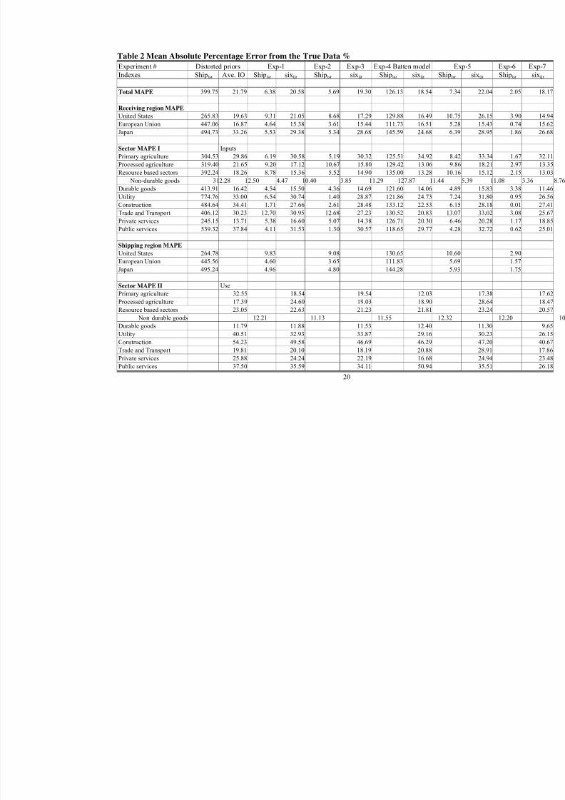
4.4 Testing results

Table 2 summarizes all the eight measurement indexes from the seven testing

experiments listed in Table 1. The accuracy of the estimates is judged by their closeness to the

true interregional trade and individual region’s input–output flows aggregated from the GTAP

database.

(Insert Table 2 here)

Generally speaking, the model has remarkable capacity to rediscover the true

interregional trade flows from the highly distorted data. The estimated shipment data are very

close to the true data by the eight types of measurement in all testing experiments except the

Batten model. Most of the mean absolute percentage errors are about 4-7 percent of the true data

value, which implies the model has great potential in the application of estimating interregional

trade flows. In contrast, recovering the individual region’s input-output flows from national

average values only obtained very limited success, indicating national detailed IO coefficients

may be the best place to start in building regional IO account if there is no additional prior

information on regional technology or cost structure available.

Comparing estimates from different test experiments, there are several interesting

observations. First, when there is no additional information that could be incorporated into the

estimation framework, a more detailed model may not perform better than a simpler model

(compare results from Exp-1 and Exp-5, the more sophisticated extended model actually bring

less accurate estimates overall because of losing degrees of freedom). However, as results in

Experiments 2-3 and 6-7 show, the estimation accuracy does improve by a more detailed model

when more useful data become available. Second, the marginal accuracy gained from actual

individual regional IO flows is significant in estimating interregional trade flow using the



19

extended model, but quite small in the aggregate version. In contrast, the marginal value of

accurate interregional shipment data is rather small in estimating individual regional IO

coefficients under both versions of the model. Finally, Batten’s model performed poorly in

interregional shipment estimation, but obtained very similar estimates on individual regional IO

flows as our model, providing further evidence that there may be no high dependency between

individual regional IO coefficients and interregional trade flows. However, caution may be

needed for a firm conclusion because the particular data set used to test the model in this paper

may be part of the problem. Since the United States, EU and Japan are all large economies, their

intermediate demands are largely meet by their own production. Therefore, the correlation

between their individual inter-industrial flow and inter-regional shipments may be particular low.

This may be responsible for the insensitivity of their IO flow estimates to changes in

interregional shipment data. In most single country regional models, inter-regional trade flows

are likely to provide a substantial share of intermediate and final demand needs within the

region.

Because the extended model only provide better estimates of interregional shipments

when individual regional IO data are available, the aggregate version of the model specified in

this paper may be the best practitioner’s tool in estimating interregional trade flows. It not only

demands less statistical information, but also has a smaller model dimension, which will

facilitate the implementation and computation process6.

6 The aggregate model only has N(NM+M2+5M) variables and N(3M+N+5) constraints, while theextended model has (N2M + NHM)(M+1) variables and N(M2+NM+N+5) constraints. This is a muchlarger model, having NM2(N-1) + NM(HM-5) more variables and MN(M+N-3) additional constraints.



Table 2 Mean Absolute Percentage Error from the True Data %

20

Experiment # Distorted priors Exp-1 Exp-2 Exp-3 Exp-4 Batten model Exp-5

Indexes Shipisr Ave. IO Shipisr sixijr Shipisr sixijr Shipisr sixijr Shipisr s

Total MAPE 399.75 21.79 6.38 20.58 5.69 19.30 126.13 18.54 7.34

Receiving region MAPEUnited States 265.83 19.63 9.31 21.05 8.68 17.29 129.88 16.49 10.75

European Union 447.06 16.87 4.64 15.38 3.61 15.44 111.73 16.51 5.28

Japan 494.73 33.26 5.53 29.38 5.34 28.68 145.59 24.68 6.39

Sector MAPE I Inputs

Primary agriculture 304.53 29.86 6.19 30.58 5.19 30.32 125.51 34.92 8.42

Processed agriculture 319.40 21.65 9.20 17.12 10.67 15.80 129.42 13.06 9.86

Resource based sectors 392.24 18.26 8.78 15.36 5.52 14.90 135.00 13.28 10.16

Non-durable goods 312.28 12.50 4.47 10.40 3.85 11.29 127.87 11.44 5.39

Durable goods 413.91 16.42 4.54 15.50 4.36 14.69 121.60 14.06 4.89

Utility 774.76 33.00 6.54 30.74 1.40 28.87 121.86 24.73 7.24

Construction 484.64 34.41 1.71 27.66 2.61 28.48 133.12 22.53 6.15

Trade and Transport 406.12 30.23 12.70 30.95 12.68 27.23 130.52 20.83 13.07Private services 245.15 13.71 5.38 16.60 5.07 14.38 126.71 20.30 6.46

Public services 539.32 37.84 4.11 31.53 1.30 30.57 118.65 29.77 4.28

Shipping region MAPE

United States 264.78 9.83 9.08 130.65 10.60

European Union 445.56 4.60 3.65 111.83 5.69

Japan 495.24 4.96 4.80 144.28 5.93

Sector MAPE II Use

Primary agriculture 32.55 18.54 19.54 12.03

Processed agriculture 17.39 24.60 19.03 18.90

Resource based sectors 23.05 22.63 21.23 21.81

Non-durable goods 12.21 11.13 11.55 12.32

Durable goods 11.79 11.88 11.53 12.40

Utility 40.51 32.93 33.87 29.16

Construction 54.23 49.58 46.69 46.29

Trade and Transport 19.81 20.10 18.19 20.88

Private services 25.88 24.24 22.19 16.68

Public services 37.50 35.59 34.11 50.94



V. Empirical Issues when the Model is applied to the US Economy

To implement the model in the context of the United States, the first task is assembling

data from different sources. This data will be used to specify the national input-output account,

sector totals of output, value-added, exports, imports and final demand at the state level as well

as initial information of inter/intra-state commodity shipments. Much of this information is

available directly from official statistical sources.

The Detailed Benchmark Input-Output Account of the United States7 is estimated every

five years, with the most recent benchmark having been published in December of 2002 by the

Bureau of Economic Analysis (BEA), based on calendar year 1997 economic statistics. As is true

for the majority of nations who maintain official national economic accounting systems, the U.S.

system of official economic statistics does not include an interregional, inter-industry accounting

system.

The benchmark account coincides with the calendar year economic statistics of the

Economic Census and Census of Governments (U.S. Dept. of Census), Census of Agriculture

(U.S. Dept. of Agriculture), and other ancillary U.S. regional economic accounts. State level

statistics on gross output, value added and/or total wage-bill are, for the most part, routinely

extracted from these sources. Other relevant statistics include annual industry gross state product

accounts (BEA), ‘origin of movement’ State export statistics and import statistics by port of

entry into the U.S. (Census)8. Finally, depending on the emphasis of the modeler’s application,

7 This ‘detailed’ account characterizes all U.S. domestic inter-industry activities for calendar year 1997,as summarized into 491 industry aggregates, 483 commodity aggregates, and U.S. GDP by commodity, broken out into personal consumption, gross private investment, net exports, inventory change, andgovernment investment and consumption.

8 Equations (2) and (3) can be modified to be consistent with those officially published export and importstatistics.

21



other Federal and State Government statistics, trade association data, and proprietary data have

useful information that will complement the primary official data sources.

State final demand statistics are the only data items that are not as routinely extracted

from primary data sources. Important indirect information that can be used to estimate State

consumer expenditures include the Bureau of Labor Statistics (BLS), Consumer Expenditure

Survey (CES), the decennial Census of Population, and Internal Revenue Service (IRS) statistics

on income. For example, using BLS regional CES tables, one can allocate U.S. expenditure data

out to one of four U.S. regions. Next, using CES expenditure statistics by household income, and

by other socioeconomic categories, one can use Census of Population State statistics to further

allocate regional expenditure estimates out to States.

For gross private investment, BEA produces detailed wealth account statistics that

include annual gross private investment by major industry groups. The Internal Revenue Service

publishes State investment and depreciation statistics that allow one to infer the level and type of

investments that business’ and households are making in each state. Combining these data with

the national private investment statistics by detailed commodity groups, one can develop

regional estimates of gross private state investment. Federal and State procurement data are

available from two comprehensive sources, the General Services Administration and the U.S.

Census of Governments. Perhaps the most elusive information is that on State inventory change.

State level information does exist for some of the 483 Commodity aggregates, and this data can

supplement estimates that assume, at the detailed commodity level, that inventory change is a

constant percentage of both national and State final demand.

The confidence of the developer in their estimates may depend on their abilities to obtain

relevant data not typically available. This data can be used to fill data gaps created by

22



deficiencies of the conventional data sources. If that confidence exists, estimates of State level

data on output, value added, imports, exports, and total final demand, by commodity, can be used

as the ‘true’ identities in solving the national system of regional input-output accounts. To the

extent that a subset of this data is considered unreliable, employing methods of attaching

reliability weights (Stone, 1982, 1988) to these suspect data points can facilitate the more general

specification of the models presented in the previous section.

Whichever approach one takes, the most challenging empirical obstacle to solving an

U.S. balanced IRIO from the model is the development of regional technical input-output

coefficient priors, and inter/intra-regional shipment data priors. Two very useful ‘rules of thumb’

can be applied to this problem and when applied together, can reinforce each other.

One often-applied ‘rule’ is known as the product mix approach (Miller & Blair, 1985, p.

70). This approach requires that, in lieu of other information on the regional technical

coefficients, estimates of the product mix for the detailed industries that map into a regional

commodity aggregate should be used. With this information, a weighted average of the national

input-output coefficients of these products, where the weights are the share of regional aggregate

commodity gross output that each detailed industry represents, produces a unique regional

coefficient for each commodity aggregate represented in the regional system.

Another useful ‘rule’ pertains to the use of aggregate transportation data. This rule states

that in lieu of detailed transportation statistics on inter/intra regional commodity flows, a regional

input-output system should be solved at a level of aggregation most closely aligned with the

aggregation reported in the transportation data. While this aggregation may be insufficient for the

specific purposes of the developer, it is likely that the developer knows of other unique data

sources related to transportation in the sectors of particular relevance to their research and this

23



data can be incorporated. For other sectors that the developer has little familiarity with, the

aggregated data will probably end up providing more information than if it was used, for

example, to move all subcategories of each commodity aggregate.

To illustrate how to use both of these ‘rules’ could complement each other, consider the

following example. Suppose annual state-to-state transportation statistics were available to a

developer designing an U.S. MRIO system for use in energy analysis. If this transportation data

described the value of shipments within and between states on ‘Food and Kindred Products’,

commodities as diverse as cotton and ice would belong to this industry aggregate. Suppose a

particular region of an MRIO system produces food and kindred products that predominantly

have similar cost structures as ice, and another region has products in this category that

predominantly have similar cost structures as cotton. Using the product mix approach, the former

region would end up with an aggregate food industry I-O coefficient for electricity that would be

considerably higher than in the later region.

Now suppose that after doing the work of developing detailed regional output data for the

product mix approach, the developer decided to keep the detail in the model they are trying to

solve. Typically, this would mean that if transportation data indicated 20-percent of region I food

and kindred product shipments went to region II, than a prior for each detailed commodity would

have 20-percent going to region II. In solving a system with such priors, it is very likely that a

substantial amount of product will be redirected, while a more aggregated system would most

likely not have as much redirection. The significance of this result is illustrated in the following

scenario.

Suppose an U.S. MRIO system includes regions of Florida and California, and one of the

commodities modeled was ‘canned fruits and vegetables’. While this is typically viewed as a

24



detailed commodity category, there is a large product variety within this group, including fresh

orange juice—a product almost unique to Florida. California produces a substantial share of the

canned vegetables. Using the aggregated transportation data priors to move canned fruits and

vegetables, both Florida and California will initially have too much canned products remaining

in State. Further, from an optimization perspective, it will be very efficient to diminish or sever

the bilateral flows of canned products between California and Florida. A developer specializing

in the energy industry is unlikely to notice this outcome. On the other hand, using the aggregated

sectors, the CA/FL trade linkage is more likely to be preserved. For most energy issues, it’s not

important to know that Florida and California are trading orange juice and canned vegetables,

but it is important to know that the two economies have a strong direct economic linkage.

Appendix III reports an U.S. MRIO system with 51 regions and 38 sectors based on the

data and approaches discussed in this section [forthcoming]. While such a system is likely to

have too much industry aggregation for most practical applications, extensions of this data set

using the procedures discussed above for the sectors of interest to the developer’s application

would be a routine extension of this approach. Evaluating the accuracy for this MRIO system is

an important topic, but is beyond the scopes of present inquiry.

VI. Conclusions and Direction for Future Research

This study constructed a mathematical programming model to estimate interregional

trade patterns and input-output accounts based on an interregional accounting framework and

initial estimates of interregional shipments in a national system of economic regions. The model

is quite flexible in its data requirement and has desirable theoretical and empirical properties. An

empirical test on the model using a 3-region, 10-sector example aggregated from version 4

25



GTAP database show that the model performed remarkably well in discovering the true patterns

of interregional trade from highly distorted initial estimates on interregional shipments. It shows

the model may have great potential in the application of estimating and reconciliation of

interregional trade flow data, which often are the most difficult part in assembling the

equilibrium base year data set for interregional CGE models. In addition, solutions from the

aggregated model exactly provide the data needed for a MRIO model and solution from the

extended model exactly provide the data needed for an IRIO model. This will greatly reduce the

data processing burden in such analysis. Therefore, application of the model will further

facilitate quantitative economic analysis in regional sciences.

However, there are important questions not yet answered by the current study. First, test

results from the data set aggregated from GTAP also show that our model’s ability to improve

the IO transaction estimates of individual regions from national average may be limited.

Continuing research on the real underlying causes and ways of improvement are needed to

further enhance the model’s capacity as an estimating and reconciliation tool in building

interregional production and trade accounts. Second, the relative importance of regional sector

output, value-added, exports, imports and final demand as model input in the accuracy of a

model solution is also not analyzed yet, and could be addressed with minor changes of the

current model. Finally, the robustness of the model performance needs further testing by using

other data sets.

26



Appendix A: Constraint Matrix Balancing problem

The model is a special case of the constrained matrix-balancing problem from a

mathematical perspective. It is so named because it involves the computation of the best estimate

of an unknown matrix from a given matrix, with some prior information to constrain the solution

set. It appears as a core structure in diverse applications. These applications include the

estimation of input-output tables (Bachem and Korte, 1981; Harrigan and Buchanan, 1984;

Miller and Blair, 1985; Kaneko, 1988; Nagurney, 1989; Antonello, 1990) and inter-regional

trade flows in regional science (Batten, 1982; Byron et al., 1993), balancing of social/national

accounts in economics (Byron, 1978; Van der Ploeg, 1982, 1984,1988; Zenios, Drud, and

Mulvey, 1989; Nagurney, Kim, and Robinson, 1990), estimating interregional migration in

demography (Plane, 1982), the analysis of voting patterns in political science (Johnson, Hay, and

Taylor, 1982), the treatment of census data and estimation of contingency tables in statistics

(Friedlander, 1961), the estimation of transition probabilities in stochastic modeling (Theil and

Rey, 1966), and the projection of traffic within telecommunication and transportation networks

(Florian, 1986; Klincewicz, 1989). A comprehensive survey can be found in Schneider and

Zenios (1990).

Methods for matrix balancing can be classified into two broad classes -- bi-proportional

scaling and optimization. The scaling methods are based on the adjustments of the initial matrix

to multiplying its row and column by positive constants until the matrix is balanced. It was

developed by Stone and other members of the Cambridge Growth Project (Stone et al., 1963)

and is usually known as RAS. The basic method was originally applied to known row and

column totals but had been extended to cases where the totals themselves are not known with

certainty (Senesen and Bates, 1988). Optimization methods are based on mathematical

27



programming, usually minimizing a penalty function, which measures the deviation of the

candidate balanced matrix from the initial matrix subject to a set of balance condition.

The scaling methods such as RAS have been one of the most widely applied

computational algorithms for the solution of the constrained matrix balancing problems. They

are simple, iterative, and require minimal programming effort to implement. However, as pointed

out by van der Ploeg (1982), they are not straightforward to use when including more general

linear restrictions and when allowing for different degrees of uncertainty in the initial estimates

and restraints. They also lack a theoretical interpretation of the adjustment process. Those

aspects are crucial for an adjustment procedure to improve the information content of the

balanced estimates rather than only adjusting the initial estimates mechanically. Mohr, Crown

and Polenske (1987) discussed the problems encountered when the RAS procedure is used to

adjust trade flow data. They pointed out that the special properties of interregional trade data

increase the likelihood of non-convergence of the RAS procedure and proposed a linear

programming approach that incorporate exogenous information to override the unfeasibility of

the RAS problem.

Since the 1980s more and more researchers have tended to formulate constrained matrix

balancing problems as mathematical programming problems (var der Ploeg, 1988, Nagurney and

Robinson, 1989, Bartholdy, 1991, Byron et al., 1993), with an objective function that forces

"conservatism" on the process of rationalizing X from the initial estimate X0. The theoretical

foundation for the approach can be viewed from both the perspectives of mathematical statistics

and information theory. When a quadratic penalty function is used, the solution of this

mathematical programming problem gives a minimum variance unbiased linear estimate of the

unknown matrix X (Byron, 1978, Van der Ploeg, 1982, 1984); while when a entropy function is

28



used, its solution gives the estimate of X which minimizes the "information added" to X 0 needed

to conform to the constraints (Wilson 1970). In addition, the solution of the RAS method is

equivalent to constrained entropy minimization with fixed prior row and column totals, as shown

by Bregman (1967), thus can been seen as a special case of the optimization methods.

Another important advantage of mathematical programming models over scaling

methods in applied matrix balancing problems is that it permits one to introduce relative degree

of reliability for the initial estimates. Further, additional constraints may be imposed on the data

adjustment process, such as allowing precise upper and lower bounds to be placed on unknown

elements, or incorporating an associated term in the objective function to penalize solution

deviations from the initial row or column total estimates when they are not known with certainty.

Therefore, it provides more flexibility to the matrix balancing procedure. This flexibility is very

important in terms of improving the information content of the balanced estimates.

The idea of including reliability of the initial estimate in the matrix balancing process can

be traced back half a century to Richard Stone and his colleagues (1942) when they explored

procedures for compiling national income accounts. Their ideas were formalized into a

mathematical procedure to balance the system of accounts after assigning reliability weights to

each entry in the system. The minimization of the sum of squares of the adjustments between

initial entries and balanced entries in the system, weighted by the reliabilities or the reciprocal of

the variances of the entries is carried out subject to linear (accounting) constraints. This approach

had first been operationlized by Byron (1978) and applied to the System of National Accounts of

UK by Ploeg (1982, 1984). Zenios and his collaborators (1989) further extended this approach to

balance a large social accounting matrix in a nonlinear network-programming framework.

29



Although computational burden is no longer a problem today, the difficulty of estimating the

error variances with this method still remains unsolved.

30



Appendix B GAMS Program for the 3-region, 10-sector Example

1. Data processing program

*This program produces a test data set for the minimum information gain model**from a 4-region 10-sector aggregation version 4 GTAP database

**## SECTORSSETS

IS / AGR,PFD,RES,CON,DUR,UTL,CNS,TAT,PSV,GSV,CGD,total /

I(IS) / AGR AGRICULTUREPFD FOOD PROCESSINGRES RESOURCE BASED SECTOR CON NON-DURABLE CONSUMER GOODSDUR DURABLE GOODSUTL UTILITYCNS CONSTRUCTIONTAT TRADE AND TRANSPORTPSV PRIVATE SERVICEGSV PUBLIC SERVICE

CGD INVESTMENT GOODS /

TTS(IS) / AGR,PFD,RES,CON,DUR,UTL,CNS,TAT,PSV,GSV,total /

T(I) / AGR,PFD,RES,CON,DUR,UTL,CNS,TAT,PSV,GSV /

II(T) / AGR,PFD,RES,CON,DUR,UTL,CNS,PSV,GSV /

JJ(T) / PFD,RES,CON,DUR,UTL,CNS,TAT,PSV,GSV /JI(T) / PFD,CON,DUR,UTL,CNS,TAT,PSV,GSV /

IOM(T) / DUR,TAT,PSV /ISV(T) / UTL,CNS,TAT,PSV,GSV /MFL(T) / PFD,CON /MFH(T) / DUR /

KK(T) / res /IAG(T) / agr /IAG1(T) / agr,pfd /

**## REGIONSrs / USA,EEC,JPN,ROW,tot /

r(rs) REGIONS / USA UNITED STATESEEC European UnionJPN JAPANROW REST OF THE WORLD /

rr(r) / USA,EEC,JPN /

**## FACTORS OF PRODUCTION

IIF FACTORS / LND LANDAGLB RURAL-LABOR ULB UNSKILLED-LABOR SLB SKILLED-LABOR CAP CAPITAL

NRS SECTOR SPECIFIC RESOURCES /

F / LND,ULB,SLB,CAP,NRS /

31



FF(IIF) / LND,ULB,SLB,CAP,NRS /FF0(FF) / LND,ULB,SLB,CAP /FC(FF) / LND,SLB,CAP /FF1(FF) / ULB,SLB,CAP /FF2(FF) / ULB,SLB,CAP,NRS /FL(F) / ULB,SLB /FR(F) / LND,CAP,NRS /

FB(FF) / LND,SLB,CAP / ;

SETS**## SET FOR CET FUNCTION CONTROL

IE1(T,R) CET AGGREGATE EXPORT SECTORS

IE2(T,R) COMPETITIVE EXPORT SECTORS

/ (agr).(USA,EEC,JPN,ROW) /

;

ALIAS (FF,FFC),(FF0,FFC0),(FF1,FFC1),(FF2,FFC2),(JJ,JJC),(FC,FCC);ALIAS (R,RT,S,ST), (rr,ss),(I,IT), (F,FT),(FL,FLT),(T,K,KC);

SETS**## OTHER SETS

MAC MACRO VARIABLES/ SAVE Regional savings

VDEP Capital DepreciationVKB Capital stock in the beginning periodHTAX Household income tax /

;

SETS MISX(T,R,S) ZERO TRADEMISE(T,R) ZERO EXPORTMISM(T,R) ZERO IMPORTMISQ(T,R) ZERO PRODUCTIONMISDF(FF,T,R) ZERO FACTOR DEMAND

MISVA(T,R) ZERO VALUE-ADDEDQOUTA(T,R,S) TRADE FLOWS SUBJECT IMPORT QOUTAS ;

*---------- BASIC DATA FROM GTAP GLOBAL TRADE DATA BASE ----------*

$INCLUDE data\gtap4.DAT

*-------------------------------DERIVED DATA FROM THE BASIC DATA -----------------------------------------------*

PARAMETER VFA(T,I,R) PRODUCER COST ON INTEMEDIATE INPUTS T BY INDUSTRY I IN REGION R AT AGENT'S PRICEVFM(T,I,R) PRODUCER COST ON INTEMEDIATE INPUTS T BY INDUSTRY I IN REGION R AT MARKET PRICEVOA(I,R) TOTAL PRODUCTION COST OF SECTOR I IN REGION R AT AGENT'S PRICEVOM(I,R) TOTAL VALUE OF OUTPUT I IN REGION R AT MARKET PRICE

EVOM(F,R) TOTAL VALUE ADDED FOR FACTOR F AT MARKET PRICEVDM(T,R) DOMESTIC SALES OF COMMODITY T IN REGION R AT MARKET PRICEVDA(T,R) DOMESTIC SALES OF COMMODITY T IN REGION R AT AGENT PRICEVPA(T,R) HOUSEHOLD EXPENDITURE ON COMMODITY T IN REGION R VALUED AT AGENT'S PRICEVPM(T,R) HOUSEHOLD EXPENDITURE ON COMMODITY T IN REGION R VALUED AT MARKET PRICEVIM(T,R) VALUE OF TOTAL IMPORTS OF COMMODITY T BY REGION R HEXP(R) HOUSEHOLD CONSUMPTION EXPENDITURE IN REGION R VGA(T,R) GOVERNMENT HOUSE HOLD EXPENDITURE ON COMMODITY T IN REGION R AT AGENT'S PRICEVGM(T,R) GOVERNMENT HOUSE HOLD EXPENDITURE ON COMMODITY T IN REGION R AT MARKEY PRICEGEXP(R) GOVERNMENT CONSUMPTION EXPENDITURE ON REGION R

32



VTW(T,R,S) TRANSPORTATION COST ASSOCIATED WITH THE SHIPMENT* OF COMMODITY T FROM REGION R TO S

ER(T,R) DIFFERENCE BETWEEN TOTAL IMPORTS AND DOMESTIC ABSORBTION* OF IMPORT GOODS, SHOULD BE ZERO

BOT(R) BALANCE OF TRADE IN REGION R CHECKA(T,R)CHECKC(T,R)

VT TOTAL COST OF INTERNATIONAL TRANSPORTATION SERVICESSAVE(R) HOUSEHOLD SAVINGSVDEP(R) DEPRECIATIONVKB(R) CAPITAL STOCK REGINV(R) GROSS REGIONAL INVESTMENT IN REGION R GSAV(R) GOVERNMENT SAVING OR DEFICIT;

PARAMETERSSAVE(R) Expenditures on net savings (AP)VDEP(R) Value of capital depreciation (AP)VKB (R) Value of beginning-of-period capital stock (AP)GTRANS0(R) GOVERNMENT SAVING OR DEFICIT;

SAVE(R) = MACRO(R,"save") ;

VDEP(R) = MACRO(R,"vdep") ;VKB (R) = MACRO(R,"vkb") ;

VFA(T,I,S) = VDFA(T,I,S) + VIFA(T,I,S);VFM(T,I,S) = VDFM(T,I,S) + VIFM(T,I,S);VOA(I,R) = SUM(T, VFA(T,I,R)) + SUM(F, EVFA(F,I,R));VDM(T,R) = VDPM(T,R) + VDGM(T,R) + SUM(I, VDFM(T,I,R));VDA(T,R) = VDPA(T,R) + VDGA(T,R) + SUM(I, VDFA(T,I,R));VOM("CGD",R) = VOA("CGD",R);VOM(T,S) = VDM(T,S) + SUM(R, VXMD(T,S,R)) + VST(T,S);EVOM(F,R)= SUM(I, EVFM(F,I,R));VPA(T,S) = VDPA(T,S) + VIPA(T,S);VPM(T,S) = VDPM(T,S) + VIPM(T,S);HEXP(R) = SUM(T, VPA(T,R));VGA(T,S) = VDGA(T,S) + VIGA(T,S);

VGM(T,S) = VDGM(T,S) + VIGM(T,S);GEXP(R) = SUM(T, VGA(T,R));SAVE(R) = MACRO(R,"SAVE");VDEP(R) = MACRO(R,"VDEP");VKB(R) = MACRO(R,"VKB");VTW(T,R,S) = VIWS(T,R,S) - VXWD(T,R,S);

BOT(R) = SUM(T,VST(T,R))+ SUM((T,S), VXWD(T,R,S)) - SUM((T,S), VIWS(T,S,R));VT = SUM((T,S,R), VTW(T,R,S));

* DISPLAY VDM, VFA, VFM, VPA,VPM,VGA,VGM;DISPLAY VOA,VOM;

* DISPLAY EVOM,HEXP,GEXP,VTW, BOT,VT;

PARAMETER PTAX(I,R) VALUE OF PRODUCT TAXDPTAX(T,R) VALUE OF CONSUMPTION TAX OF DOMESTIC GOODS BY HOUSEHOLDIPTAX(T,R) VALUE OF CONSUMPTION TAX OF IMPORTS BY HOUSEHOLDDGTAX(T,R) VALUE OF CONSUMPTION TAX OF DOMESTIC GOODS BY GOVERNMENTIGTAX(T,R) VALUE OF CONSUMPTION TAX OF IMPORTS BY GOVERNMENTDFTAX(T,I,R) VALUE OF CONSUMPTION TAX OF DOMESTIC GOODS BY FIRMSIFTAX(T,I,R) VALUE OF CONSUMPTION TAX OF IMPORTS BY FIRMS

XTAX(T,R,S) VALUE OF EXPORT TAXMTAX(T,S,R) VALUE OF TARRIFF

33



ETAX(F,R) VALUE OF FACTOR TAXHTAX(R) VALUE OF HOUSEHOLD INCOME TAXITAX(I,R) VALUE OF FIRM INPUT TAXCTAX(T,R) VALUE OF CONSUMPTION TAXKTAX(T,R) VALUE OF CAPITAL GOODS TAX;

DPTAX(T,R) = VDPA(T,R)-VDPM(T,R);

IPTAX(T,R) = VIPA(T,R)-VIPM(T,R);DGTAX(T,R) = VDGA(T,R)-VDGM(T,R);IGTAX(T,R) = VIGA(T,R)-VIGM(T,R);DFTAX(T,I,R) = VDFA(T,I,R)-VDFM(T,I,R);IFTAX(T,I,R) = VIFA(T,I,R)-VIFM(T,I,R);

PTAX(I,R) = VOM(I,R)-VOA(I,R);XTAX(T,R,S) = VXWD(T,R,S) - VXMD(T,R,S);MTAX(T,S,R) = VIMS(T,S,R) - VIWS(T,S,R);

ETAX(F,R) = SUM(I, (EVFA(F,I,R) - EVFM(F,I,R)));HTAX(R) = SUM(F, (EVOM(F,R) - EVOA(F,R)));

CTAX(T,R) = DPTAX(T,R) + IPTAX(T,R) + DGTAX(T,R) + IGTAX(T,R)+ IFTAX(T,"CGD",R) + DFTAX(T,"CGD",R);

ITAX(T,R) = SUM(K, (IFTAX(K,T,R) + DFTAX(K,T,R)));

DISPLAY PTAX,XTAX,MTAX,ETAX,HTAX,CTAX,ITAX;

*------------- CHECKING THE BENCHMARK DATA FROM GTAP DATABASE -----------------*

PARAMETER

PROFITS(I,R) PROFITS INSECTOR I OF REGION R, SHOULD BE ZEROSURPLUS(R) ECONOMIC SUPLUS IN REGION R, SHOULD BE ZEROACTER(T,R)RESBOTTSR RESIDUAL OF INTERNATIONAL TRANSPORTATION INDUSTRY, SHOULD BE ZERO;

PROFITS(I,R) = VOA(I,R) - SUM(T,VFA(T,I,R)) - SUM(F, EVFA(F,I,R));

ACTER(T,R) = VOM(T,R) - VDM(T,R) - SUM(S, VXMD(T,R,S)) - VST(T,R);

VIM(T,R) = SUM(I, VIFM(T,I,R)) + VIPM(T,R) + VIGM(T,R);ER(T,R) = VIM(T,R) - SUM(S, VIMS(T,S,R));

SURPLUS(R) = SUM(F,EVOA(F,R))- VDEP(R) + SUM(I,PTAX(I,R)) + SUM(T,CTAX(T,R))+ SUM(T,ITAX(T,R)) + SUM((T,S), (XTAX(T,R,S) + MTAX(T,S,R)))+ SUM(F,ETAX(F,R)) + HTAX(R) - SUM(T,(VPA(T,R)+VGA(T,R))) - SAVE(R);

TSR=SUM((T,R), VST(T,R)) - VT;RESBOT=SUM(R, BOT(R));

DISPLAY RESBOT,TSR,ER,PROFITS,ACTER,SURPLUS;

GSAV(R) = SUM(T, PTAX(T,R)) + SUM((K,S),(MTAX(K,S,R)+XTAX(K,R,S)))+ SUM(T,(CTAX(T,R)+ITAX(T,R))) + SUM(F,ETAX(F,R)) + HTAX(R) - GEXP(R);

*## eliminate intra-regional trade flows

PARAMETERS

INTSHIPW(T,R) INTRA-REGIONAL SHIPPING SERVICES AT WORLD PRICEINTTAXM(T,R) INTRA-REGIONAL IMPORT TAXINTTAXE(T,R) INTRA-REGIONAL EXPORT TAXVIA(T,R) VALUE OF INVESTMENT BY SECTOR AND BY REGION

34



VPAWT(T,R) SHARE OF HOUSEHOLD CONSUMPTION IN FINAL DEMAND BY SECTOR VGAWT(T,R) SHARE OF GOVERNMENT SPENDING IN FINAL DEMAND BY SECTOR VIAWT(T,R) SHARE OF INVESTMENT IN FINAL DEMAND BY SECTOR;

VPAWT(T,R)$(VPA(T,R)+VGA(T,R)+VFA(T,"CGD",R)) = VPA(T,R)/(VPA(T,R)+VGA(T,R)+VFA(T,"CGD",R));VGAWT(T,R)$(VPA(T,R)+VGA(T,R)+VFA(T,"CGD",R)) = VGA(T,R)/(VPA(T,R)+VGA(T,R)+VFA(T,"CGD",R));VIAWT(T,R)$(VPA(T,R)+VGA(T,R)+VFA(T,"CGD",R)) = VFA(T,"CGD",R)/(VPA(T,R)+VGA(T,R)+VFA(T,"CGD",R));

INTSHIPW(T,R)= VIWS(T,R,R)-VXWD(T,R,R);INTTAXM(T,R) = VIMS(T,R,R) - VIWS(T,R,R);INTTAXE(T,R) = VXWD(T,R,R) - VXMD(T,R,R);VST("tat",R) = VST("tat",R) - SUM(T,INTSHIPW(T,R));CTAX(T,R) = CTAX(T,R) + INTTAXM(T,R) + INTTAXE(T,R);VDM(T,R) = VDM(T,R) + VXWD(T,R,R) - INTTAXE(T,R);VDM("tat",R) = VDM("tat",R) + SUM(T,INTSHIPW(T,R));VDM("tat","ROW") = VDM("tat","ROW") + TSR;VST("tat","ROW") = VST("tat","ROW") - TSR;VDA(T,R) = VDA(T,R) + VXWD(T,R,R) - INTTAXE(T,R);VDA("tat",R) = VDA("tat",R) + SUM(T,INTSHIPW(T,R));VDA("tat","ROW") = VDA("tat","ROW") + TSR;

VPA(T,R) = VPA(T,R) - VPAWT(T,R)*INTSHIPW(T,R);

VIPM(T,R) = VIPM(T,R) - VPAWT(T,R)*VIMS(T,R,R) ;VGA(T,R) = VGA(T,R) - VGAWT(T,R)*INTSHIPW(T,R);VIGM(T,R) = VIGM(T,R)-VGAWT(T,R)* VIMS(T,R,R);VIFM(T,"CGD",R) = VIFM(T,"CGD",R) - VIAWT(T,R)* VIMS(T,R,R);

VFA(T,"CGD",R) = VFA(T,"CGD",R) - VIAWT(T,R)*INTSHIPW(T,R);VPA("tat",R) = VPA("tat",R) + SUM(T,VPAWT(T,R)*INTSHIPW(T,R));VGA("tat",R) = VGA("tat",R) + SUM(T,VGAWT(T,R)*INTSHIPW(T,R));VFA("tat","CGD",R) = VFA("tat","CGD",R) + SUM(T,VIAWT(T,R)*INTSHIPW(T,R));VIA(T,R) = VFA(T,"CGD",R);DISPLAY INTTAXM,INTTAXE,INTSHIPW, VGA,VPA,VIA;

VIMS(T,R,R) = 0.0;VIWS(T,R,R) = 0.0;VXMD(T,R,R) = 0.0;

VXWD(T,R,R) = 0.0;XTAX(T,R,R) = 0.0;MTAX(T,R,R) = 0.0;VTW(T,R,R) = 0.0;

VT = SUM((T,S,R), VTW(T,R,S));TSR=SUM((T,R), VST(T,R)) - VT ;DISPLAY TSR;

save(r) = save(r) + surplus(r);

*## RE-CHECK DATA CONSISTANCY AFTER ADJUSTMENTS

SURPLUS(R) = SUM(F,EVOA(F,R))- VDEP(R) + SUM(I,PTAX(I,R)) + SUM(T,CTAX(T,R))+ SUM((T,S), (XTAX(T,R,S) + MTAX(T,S,R)))+ SUM(F,ETAX(F,R)) + HTAX(R) - SUM(T,(VPA(T,R)+VGA(T,R))) - SAVE(R);

VIM(T,R) = SUM(I, VIFM(T,I,R)) + VIPM(T,R) + VIGM(T,R);ER(T,R) = VIM(T,R) - SUM(S, VIMS(T,S,R));

DISPLAY ER,SURPLUS;

*## RE-CALCULATION GOVERNMENT TRANSFER AND BALANCE OF TRADE AFTER ADJUSTMENTS

GTRANS0(R) = SUM(T, PTAX(T,R)) + SUM((K,S),(MTAX(K,S,R)+XTAX(K,R,S)))+ SUM(T,CTAX(T,R)) + SUM(F,ETAX(F,R)) + HTAX(R) - GEXP(R);

35



BOT(R) = SUM(T,VST(T,R))+ SUM((T,S), VXWD(T,R,S)) - SUM((T,S), VIWS(T,S,R));

*--------------CONSTRUCTION OF SOCIAL ACCOUNTING MATRIX---------------*

SETS

SI / ACT,COMD,FLD,FLB,FK,ENT,PH,GV,KA,WT,ITR,TOTAL/SIT(SI) /TOTAL/S1(SI) / ENT,GV,PH,KA,WT,ITR /SSI(S1) / WT,ITR /SI1(SI);

ALIAS(SI1,SI2);

PARAMETER

SAM(R,SI,SI) SOCIAL ACCOUNTING MATRIXRES(SI,R) RESIDUAL OF REVENUE AND EXPENDITURE, SHOULD BE ZERO;

SI1(SI) = NOT SIT(SI);

* FIRST BLOCK: ACTIVITIES. DOMESTIC SUPPLY,EXPORT SUBSIDY, EXPORTS AT MP* EXPORTS FOR INTERNATIONAL TRANSPORTATION.

SAM(R,"ACT","COMD") = SUM(T, VDM(T,R)) ;SAM(R,"ACT","GV") = -SUM((T,S), (VXWD(T,R,S) - VXMD(T,R,S)));SAM(R,"ACT", "WT") = SUM((T,S), VXWD(T,R,S));SAM(R,"ACT","ITR") = SUM(T,VST(T,R));

* SECOND BLOCK: COMMODITIES. INTERMEDIATE DEMAND,HOUSEHOLD CONSUMPTION,* GOVERNMENT CONSUMPTION,INVESTMENT.

SAM(R,"COMD","ACT") = SUM((T,K), VFA(T,K,R));SAM(R,"COMD","PH") = SUM(T, VPA(T,R));SAM(R,"COMD","GV") = SUM(T, VGA(T,R));SAM(R,"COMD","KA") = SUM(T, VFA(T,"CGD",R));

* THIRD BLOCK: VALUE ADDEDSAM(R,"FLD","ACT") = SUM(I, EVFM("LND",I,R));SAM(R,"FLB","ACT") = SUM(I, EVFM("ULB",I,R)) + SUM(I, EVFM("SLB",I,R));SAM(R,"FK","ACT") = SUM(I, EVFM("CAP",I,R)) + SUM(I, EVFM("NRS",I,R));

* FOURTH BLOCK: ENTERPRISE. CAPITAL INCOME AND DEPRECIATION.

SAM(R,"ENT","FK") = EVOM("CAP",R) + EVOM("NRS",R);SAM(R,"ENT","PH") = VDEP(R);

* FIFTH BLOCK: HOUSEHOLDS. INCOME FROM FACTORS.

SAM(R,"PH","FLD") =EVOM("LND",R);SAM(R,"PH","FLB") =SUM(T,EVFM("ULB",T,R)) + SUM(T,EVFM("SLB",T,R));SAM(R,"PH","ENT") = EVOM("CAP",R) + EVOM("NRS",R);

* SIXTH BLOCK: GOVERNMENT. INDIRECT TAX,TARIFFS,FACTOR TAX,CAPITAL RETURN* HOUSEHOLD TAX,NET TRANSFER AMONG GOVERNMENT.

SAM(R,"GV","FLD") = ETAX("LND",R);SAM(R,"GV","FLB") = ETAX("ULB",R) + ETAX("SLB",R);SAM(R,"GV","FK") = ETAX("CAP",R) + ETAX("NRS",R);SAM(R,"GV","PH") = HTAX(R) - GSAV(R);

36





imp importsoutput gross output

lab conpensation to employeecap capitaltax other value-added /

fd(df) / hhs,gov,inv /

va(df) / lab,cap,tax /;

parameter stateinf(r,t,df), NX(t,k),NFD(t,df)ship0(t,s,r) total shipment from region s to region r

NTX(i) National total gross output in sector i NEX(i) National exports in sector i NMX(i) National imports in sector i NTY(i) National total final demand for sector i NVA(i) National value-added in sector iSTX0(i,r) State total gross output in sector iSEX0(i,r) State exports in sector iSMX0(i,r) State imports in sector iSTY0(i,r) State total final demand for sector iSVA0(i,r) State value-added in sector ichkrows(i) Row residuals

chkcols(i) Column residualschkship(i,r);

stateinf(r,t,"hhs") = VPA(t,r);stateinf(r,t,"gov") = VGA(t,r);stateinf(r,t,"inv") = VFA(T,"CGD",r);stateinf(r,t,"exp") = VIMS(t,r,"row");stateinf(r,t,"imp") = VIMS(T,"row",R);stateinf(r,t,"lab") = SUM(fl, EVFA(fl,T,R));stateinf(r,t,"cap") = SUM(fr, EVFA(fr,T,R));stateinf(r,t,"tax") = PTAX(t,r);stateinf(r,t,"output") = VOM(t,r);

ship0(t,s,r) = VIMS(T,S,R) ;

ship0(t,r,r) = VDA(t,r) ;

STX0(t,r) = STATEINF(r,t,"output") ;SEX0(t,r) = STATEINF(r,t,"exp") ;SMX0(t,r) = MAX(0,STATEINF(r,t,"imp")) ;SVA0(t,r) = sum(va, STATEINF(r,t,va)) ;STY0(t,r) = SUM(fd,STATEINF(r,t,fd)) ;

positive variablesSTX(t,r) State total gross output in sector iSEX(t,r) State exports in sector iSMX(t,r) State imports in sector iSTY(t,r) State total final demand for sector iSVA(t,r) State value-added in sector iSHIP(t,s,r)STIO(t,k,r);

VariablesIOQ(t,k,r)txq(t,r)exq(t,r)mxq(t,r)vaq(t,r)fdq(t,r)spq(t,s,r)

38



ss1 ;

STX.L(t,r) = STX0(t,r);SEX.L(t,r) = SEX0(t,r);SMX.L(t,r) = SMX0(t,r);STY.L(t,r) = STY0(t,r);SVA.L(t,r) = SVA0(t,r);

STIO.L(t,k,r) = VFA(t,k,r);SHIP.L(t,s,r) = ship0(t,s,r);

Equationscolbal(t,r)rowbal(t,r)shipbal(t,r)ioeq(t,k,r)txeq(t,r)exeq(t,r)mxeq(t,r)vaeq(t,r)fdeq(t,r)spqeq(t,s,r)obj;

colbal(t,r).. SUM(k, stio(k,t,r)) + SVA(t,r) =E= STX(t,r);rowbal(t,rr).. SUM(k, stio(t,k,rr)) + STY(t,rr) =E= SMX(t,rr)+ SUM(ss,ship(t,ss,rr)) ;shipbal(t,rr).. SUM(ss,ship(t,rr,ss)) + SEX(t,rr) =E= STX(t,rr);ioeq(t,k,r).. IOQ(t,k,r) =E= stio(t,k,r) - VFA(t,k,r);txeq(t,r).. txq(t,r) =E= STX(t,r) - STX0(t,r);exeq(t,r).. exq(t,r) =E= SEX(t,r) - SEX0(t,r);mxeq(t,r).. mxq(t,r) =E= SMX(t,r) - SMX0(t,r);vaeq(t,r).. vaq(t,r) =E= SVA(t,r) - SVA0(t,r);fdeq(t,r).. fdq(t,r) =E= STY(t,r) - STY0(t,r);spqeq(t,ss,rr).. spq(t,ss,rr) =E= ship(t,ss,rr)- ship0(t,ss,rr);

obj.. SS1 =E= SUM((t,k,r)$VFA(t,k,r),SQR(IOQ(t,k,r))/VFA(t,k,r))+ SUM((t,r)$STX0(t,r), SQR(txq(t,r))/stx0(t,r))+ SUM((t,r)$SEX0(t,r), SQR(exq(t,r))/sex0(t,r))

+ SUM((t,r)$SMX0(t,r), SQR(mxq(t,r))/smx0(t,r))+ SUM((t,r)$SVA0(t,r), SQR(vaq(t,r))/sva0(t,r))+ SUM((t,r)$STY0(t,r), SQR(fdq(t,r))/sty0(t,r))+ SUM((t,ss,rr)$ship0(t,ss,rr),SQR(SPQ(t,ss,rr))/ship0(t,ss,rr));

*## Model solusion

OPTIONS ITERLIM=1500000,LIMROW=0,LIMCOL=0,SOLPRINT=OFF;

MODEL databal / colbalrowbalshipbalioeqtxeqexeqmxeqvaeqfdeqspqeqobj / ;

OPTIONS NLP=pathnlp;DATAbal.OPTFILE=1;SOLVE databal USING NLP MINIMIZING SS1;

NX(t,k) = SUM(rr, STIO.L(t,k,rr));

39



NTX(t) = SUM(rr, STX.L(t, rr)); NEX(t) = SUM(rr, SEX.L(t, rr)); NMX(t) = SUM(rr, SMX.L(t, rr)); NVA(t) = SUM(rr, SVA.L(t, rr)); NTY(t) = SUM(rr, STY.L(t, rr));

chkrows(t) = SUM(k, NX(t,k)) + NEX(t) + NTY(t) - NMX(t) - NTX(t);

chkcols(t) = SUM(k, NX(k,t)) + NVA(t) - NTX(t);chkship(t,rr)= SUM(ss, ship.l(t,rr,ss)) + SEX.L(t,rr) - STX.L(t,rr);

*chkrows(t) = round (chkrows(t),2) ;*chkcols(t) = round (chkcols(t),2) ;DISPLAY chkrows, chkcols,chkship ;

*---Putting the GTAP data to GAMS data file --------------------------file DATAOUT / E:\GAMSMO~1\region\data\GTAPtest.DAT / ;DATAOUT.PW = 255 ; PUT dataout ;PUT '*## DATA FROM GTAP95 DATA BASE ' //;PUT '*CREATED FROM '; PUT SYSTEM.IFILE; PUT ' ON '; PUT SYSTEM.DATE ;PUT ' AT '; PUT SYSTEM.TIME //;

* National IO flows

PUT 'TABLE NX(i,j) IO flows at national level' // ;PUT @10, LOOP( k, PUT k.TL:>20); PUT //;LOOP(t,

PUT t.TL @10 ;LOOP(k, PUT NX(t,k):20:8 ) ;PUT / ;

);PUT /;PUT@3,';' ; PUT / ;PUT /;

* regional IO flows

PUT 'Table STIO0 (i,j,r) Initial regional IO flows ' // ;PUT @14, LOOP( rr, PUT rr.TL:>23); PUT //;LOOP((t,k), PUT t.TL @6 ; PUT "." @7 ;

PUT k.TL @14 ;LOOP(rr, PUT stio.l(t,k,rr):23:11 ) ;

PUT / ;);

PUT /;PUT@3,';' ; PUT / ;PUT /;

* regional value-added

PUT 'Table SVA0(i,r) regional value-added by sector' // ;PUT @10, LOOP( rr, PUT rr.TL:>23); PUT //;LOOP(t,

PUT t.TL @10 ;LOOP(rr, PUT SVA.L(t,rr):23:11 ) ;PUT / ;

);PUT /;PUT@3,';' ; PUT / ;PUT /;

* regional final demand

40



PUT 'Table STY0(i,r) regional final demand by sector' // ;PUT @10, LOOP( rr, PUT rr.TL:>23); PUT //;LOOP(t,

PUT t.TL @10 ;LOOP(rr, PUT STY.L(t,rr):23:11 ) ;PUT / ;

);PUT /;PUT@3,';' ; PUT / ;PUT /;

* regional total output

PUT 'Table STX0(i,r) regional total output by sector' // ;PUT @10, LOOP( rr, PUT rr.TL:>23); PUT //;LOOP(t,

PUT t.TL @10 ;LOOP(rr, PUT STX.L(t,rr):23:11 ) ;PUT / ;

);PUT /;

PUT@3,';' ; PUT / ;PUT /;

* regional exports

PUT 'Table SEX0(i,r) regional exports by sector' // ;PUT @10, LOOP( rr, PUT rr.TL:>23); PUT //;LOOP(t,

PUT t.TL @10 ;LOOP(rr, PUT SEX.L(t,rr):23:11 ) ;PUT / ;

);PUT /;PUT@3,';' ; PUT / ;PUT /;

* regional imports

PUT 'Table SMX0(i,r) regional imports by sector' // ;PUT @10, LOOP( rr, PUT rr.TL:>23); PUT //;LOOP(t,

PUT t.TL @10 ;LOOP(rr, PUT SMX.L(t,rr):23:11 ) ;PUT / ;

);PUT /;PUT@3,';' ; PUT / ;PUT /;

* Inter-regional trade flows

PUT 'Table ship0(i,s,r) original inter-regional trade flow data ' // ;PUT @14, LOOP( rr, PUT rr.TL:>23); PUT //;LOOP((ss,t), PUT t.TL @6 ; PUT "." @7 ;

PUT ss.TL @14 ;LOOP(rr, PUT ship.l(T,SS,RR):23:11 ) ;

PUT / ;);

PUT /;PUT@3,';' ; PUT / ;

41



PUT /;

2. The minimum information gain model program

$OFFSYMLIST OFFSYMXREF

*## This program implement minimum information gain procedure

*## to estimate interregional, interindustry transaction flows in a national system

*## of regions based on a regional accounting framework and limited regional statistic

*## data. The complete national IO table, regional sectoral data on gross output,

*## value-added, exports, imports and final demand are used as inputs to generate

*## interregional pattern of shipment from limited information.

*---------------------- SET DEFINITION ------------------------*

$INCLUDE setgtap.inc

*---------- READ US 1997 BENCHMARK IO TABLE FROM BEA ----------*

PARAMETERS

*NX(i,j) National IO flows (input from sector i to sector j)

NTX(i) National total gross output in sector i

NEX(i) National exports in sector i

NMX(i) National imports in sector i

NTY(i) National total final demand for sector i

NVA(i) National value-added in sector i

chkrows(i) Row residuals

chkcols(i) Column residuals

chkship(i,r) residual of shipment ;

$INCLUDE data/GTAPTEST.dat

NX(i,j) = SUM(r, STIO0(i,j,r));

NTX(i) = SUM(r, STX0(i, r));

NEX(i) = SUM(r, SEX0(i, r));

NMX(i) = SUM(r, SMX0(i, r));

NVA(i) = SUM(r, SVA0(i, r));

NTY(i) = SUM(r, STY0(i, r));

*# Check balance of the national IO table

chkrows(i) = SUM(j, NX(i,j)) + NEX(i) + NTY(i) - NMX(i) - NTX(i);

chkcols(i) = SUM(j, NX(j,i)) + NVA(i) - NTX(i);

chkship(i,r)= SUM(s, ship0(i,r,s)) + SEX0(i,r) - STX0(i,r) ;

*chkrows(t) = round (chkrows(t),2) ;

*chkcols(t) = round (chkcols(t),2) ;

DISPLAY chkrows, chkcols,chkship ;

*## assign coefficient in the objective function for QP

parameters

TXQ(i,r)

TYQ(i,r)

EXQ(i,r)

MXQ(i,r)

VAQ(i,r)

SPQ(i,s,r)

IOQ(i,j,r);

42



SCALAR Qscal 'coefs of Q range from [Qscal - 1/Qscal]' / 1e-3 /;

TXQ(i,r)$STX0(i,r) = MAX[Qscal,1/MAX(STX0(i,r),Qscal)];

TYQ(i,r)$STY0(i,r) = MAX[Qscal,1/MAX(STY0(i,r),Qscal)];

EXQ(i,r)$SEX0(i,r) = MAX[Qscal,1/MAX(SEX0(i,r),Qscal)];

MXQ(i,r)$SMX0(i,r) = MAX[Qscal,1/MAX(SMX0(i,r),Qscal)];

VAQ(i,r)$SVA0(i,r) = MAX[Qscal,1/MAX(SVA0(i,r),Qscal)];

SPQ(i,s,r)$ship0(i,s,r) = MAX[Qscal,1/MAX(SHIP0(i,s,r),Qscal)];

IOQ(i,j,r)$stio0(i,j,r) = MAX[Qscal,1/MAX(STIO0(i,j,r),Qscal)];

*---------- READ KNOWN REGIONAL DATA FROM VARIOUS SOURCES ----------*

PARAMETERS

checka(i,r)

checkc(i,r)

chkship(i,r)

shipr(i,s,r) Distored interregional shipment data

stior(i,j,r) regional IO flows by aveage IO coefficients

er(i,s,r) error term

;

*## generate distored data

er(i,s,r) = 5*ship0(i,s,r) ;

shipr(i,s,r) = ship0(i,s,r) + abs(normal(0,er(i,s,r)));

*shipr(i,s,r)$(shipr(i,s,r) le 0) = ship0(i,s,r) + abs(normal(0,er(i,s,r)));

stior(i,j,r)= (STX0(i,r)-SVA0(i,r))*(NX(i,j)/(NTX(i)-NVA(i)));

display ship0, shipr;

positive variables

STX(i,r) State total gross output in sector i

SEX(i,r) State exports in sector i

SMX(i,r) State imports in sector i

STY(i,r) State total final demand for sector i

SVA(i,r) State value-added in sector iSHIP(i,s,r) Inter-state shipment

STIO(i,k,r) Indivadual region IO flows;

Variables

QIX(i,j,r)

Qtx(i,r)

Qex(i,r)

Qmx(i,r)

Qva(i,r)

Qfd(i,r)

Qsp(i,s,r)

ss1 ;

*## Variable initiation

STX.L(i,r) = STX0(i,r);

SEX.L(i,r) = SEX0(i,r);

SMX.L(i,r) = SMX0(i,r);

STY.L(i,r) = STY0(i,r);

SVA.L(i,r) = SVA0(i,r);

STIO.L(i,j,r) = stior(i,j,r);

SHIP.L(i,s,r) = shipr(i,s,r);

Equations

colbal(i,r) Sum of intermediate and factor input equals each sector output in each region

43



rowbal(i,r) Sum of intermediate and final demand equals shipment from all region plus imports

shipbal(i,r) Sum of shipment to all region and export equals the region's output

NIOBAL(i,j) Sum IO flows from sector i to sector j for all state equal the national totals

NFDBAL(i) Sum final demand of commodity i delivered by each state equal to national totals

NMAKBAL(i) Sum of output for sector i by each state equal to national output in sector i

NEXPBAL(i) Sum of exports of commodity i by each state equal to total national exports

NIMPBAL(i) Sum of imports of commodity i by each state equal to total national imports

NVABAL(i) Sum of value-added of each state equal to total national exports

ioeq(i,k,r)

txeq(i,r)

exeq(i,r)

mxeq(i,r)

vaeq(i,r)

fdeq(i,r)

spqeq(i,s,r)

obj

objetr

objqp;

colbal(i,r).. SUM(j, stio(j,i,r)) + SVA(i,r) =E= STX(i,r);

rowbal(i,r).. SUM(j, stio(i,j,r)) + STY(i,r) =E= SMX(i,r) + SUM(s,ship(i,s,r));

shipbal(i,r).. SUM(s,ship(i,r,s)) + SEX(i,r) =E= STX(i,r) ;

NIOBAL(i,j).. NX(i,j) =E= SUM(r, STIO(i,j,r)) ;NFDBAL(i).. NTY(i) =E= SUM(r, STY(i,r)) ;

NMAKBAL(i).. NTX(i) =E= SUM(r, STX(i,r)) ;

NEXPBAL(i).. NEX(i) =E= SUM(r, SEX(i,r)) ;

NIMPBAL(i).. NMX(i) =E= SUM(r, SMX(i,r)) ;

NVABAL(i).. NVA(i) =E= SUM(r, SVA(i,r)) ;

ioeq(i,j,r).. QIX(i,j,r) =E= stio(i,j,r)- stior(i,j,r);

spqeq(i,s,r).. Qsp(i,s,r) =E= ship(i,s,r)- shipr(i,s,r);

txeq(i,r).. Qtx(i,r) =E= STX(i,r) - STX0(i,r);

exeq(i,r).. Qex(i,r) =E= SEX(i,r) - SEX0(i,r);

mxeq(i,r).. Qmx(i,r) =E= SMX(i,r) - SMX0(i,r);

vaeq(i,r).. Qva(i,r) =E= SVA(i,r) - SVA0(i,r);

fdeq(i,r).. Qfd(i,r) =E= STY(i,r) - STY0(i,r);

obj.. SS1 =E= SUM((i,j,r)$STIOr(i,j,r),SQR(QIX(i,j,r))/stior(i,j,r))

+ SUM((i,s,r)$shipr(i,s,r),SQR(QSP(i,s,r))/shipr(i,s,r))

+ SUM((i,r)$STX0(i,r), SQR(Qtx(i,r))/stx0(i,r))

+ SUM((i,r)$SEX0(i,r), SQR(Qex(i,r))/sex0(i,r))

+ SUM((i,r)$SMX0(i,r), SQR(Qmx(i,r))/smx0(i,r))

+ SUM((i,r)$SVA0(i,r), SQR(Qva(i,r))/sva0(i,r))

+ SUM((i,r)$STY0(i,r), SQR(Qfd(i,r))/sty0(i,r));

OBJQP.. SS1 =E= 0 ;

*## Model solusion

OPTIONS ITERLIM=1500000,LIMROW=0,LIMCOL=0,SOLPRINT=OFF;

MODEL databal / colbal

rowbal

shipbal

NIOBAL, NFDBAL

NMAKBAL, NEXPBAL, NIMPBAL, NVABAL,

ioeq

txeq

exeq

mxeq

vaeq

44



fdeq

spqeq

obj / ;

MODEL databaletr / colbal

rowbal

shipbal

NIOBAL, NFDBAL


objetr / ;

MODEL databalqp / colbal

rowbal

shipbal

NIOBAL, NFDBAL


ioeq

txeq

exeq

mxeq

vaeq

fdeq

spqeq

objqp / ;

file qp / qmatrix.txt /;

qp.pc=5;qp.nr=2;qp.nd=10;qp.nw=0;

put qp 'Q Matrix for %system.fn%';

loop{(i,j,s,r),

put / 'QIX' i.tl j.tl r.tl 'QIX' i.tl j.tl r.tl IOQ(i,j,r);

};

loop{(i,s,r),

put / 'QSP' i.tl s.tl r.tl 'QSP' i.tl s.tl r.tl SPQ(i,s,r);

};

loop{(i,r),

put / 'QTX' i.tl r.tl 'QTX' i.tl r.tl TXQ(i,r);

};loop{(i,r),

put / 'QEX' i.tl r.tl 'QEX' i.tl r.tl EXQ(i,r);

};

loop{(i,r),

put / 'QMX' i.tl r.tl 'QMX' i.tl r.tl MXQ(i,r);

};

loop{(i,r),

put / 'QVA' i.tl r.tl 'QVA' i.tl r.tl VAQ(i,r);

};

loop{(i,r),

put / 'QTY' i.tl r.tl 'QTY' i.tl r.tl TYQ(i,r);

};

putclose;

OPTIONS NLP=pathnlp;* DATAbal.OPTFILE=1;

* SOLVE databal USING NLP MINIMIZING SS1;

* OPTIONS NLP=conopt2;

* OPTIONS NLP=snopt;

SOLVE databal USING NLP MINIMIZING SS1;

*SOLVE databalqp USING LP MINIMIZING SS1;

*ship.fx(i,s,r) = ship0(i,s,r) ;

45



*stio.fx(i,j,r) = stio0(i,j,r) ;

STX.fx(i,r) = STX0(i,r);

SEX.fx(i,r) = SEX0(i,r);

SMX.fx(i,r) = SMX0(i,r);

STY.fx(i,r) = STY0(i,r);

SVA.fx(i,r) = SVA0(i,r);

*## calculate MAPE index

parameters serror0(i,s,r), serror(i,s,r), ierror0(i,j,r), ierror(i,j,r);

ierror0(i,j,r)$stio0(i,j,r) = 100*ABS(stior(i,j,r)-stio0(i,j,r))/stio0(i,j,r);

ierror(i,j,r)$stio.l(i,j,r) = 100*ABS(stio.l(i,j,r)-stio0(i,j,r))/stio0(i,j,r);

serror0(i,s,r)$ship0(i,s,r) = 100*ABS(shipr(i,s,r)-ship0(i,s,r))/ship0(i,s,r);

serror(i,s,r)$ship0(i,s,r) = 100*ABS(ship.l(i,s,r)-ship0(i,s,r))/ship0(i,s,r);

DISPLAY serror0, serror, ierror0, ierror;

parameters MAPE(*) Total mean absolute percentage error

MAPERS(r,*) Mean absolute percentage by sending region

MAPERR(r,*) Mean absolute percentage error by receiving region

MAPEI(i,*) Mean absolute percentage error by commodity

MAPEU(i,*) ;

MAPE("distored s") = 100*SUM((i,s,r),ABS(shipr(i,s,r)-

ship0(i,s,r)))/SUM((i,s,r),ship0(i,s,r));

MAPE("estimate s") = 100*SUM((i,s,r),ABS(ship.l(i,s,r)-

ship0(i,s,r)))/SUM((i,s,r),ship0(i,s,r));

MAPERs(r,"distored s") = 100*SUM((i,s),ABS(shipr(i,r,s)-ship0(i,r,s)))/SUM((i,s),ship0(i,r,s));

MAPERs(r,"estimate s") = 100*SUM((i,s),ABS(ship.l(i,r,s)-ship0(i,r,s)))/SUM((i,s),ship0(i,r,s));

MAPERr(r,"distored s") = 100*SUM((i,s),ABS(shipr(i,s,r)-ship0(i,r,s)))/SUM((i,s),ship0(i,s,r));

MAPERr(r,"estimate s") = 100*SUM((i,s),ABS(ship.l(i,s,r)-ship0(i,s,r)))/SUM((i,s),ship0(i,s,r));

MAPEI(i,"distored s") = 100*SUM((s,r),ABS(shipr(i,s,r)-ship0(i,s,r)))/SUM((s,r),ship0(i,s,r));

MAPEI(i,"estimate s") = 100*SUM((s,r),ABS(ship.l(i,s,r)-ship0(i,s,r)))/SUM((s,r),ship0(i,s,r));

MAPE("distored i") = 100*SUM((i,j,r),ABS(stior(i,j,r)-

stio0(i,j,r)))/SUM((i,j,r),stio0(i,j,r));

MAPE("estimate i") = 100*SUM((i,j,r),ABS(stio.l(i,j,r)-

stio0(i,j,r)))/SUM((i,j,r),stio0(i,j,r));

MAPERr(r,"distored i") = 100*SUM((i,j),ABS(stior(i,j,r)-stio0(i,j,r)))/SUM((i,j),stio0(i,j,r));MAPERr(r,"estimate i") = 100*SUM((i,j),ABS(stio.l(i,j,r)-stio0(i,j,r)))/SUM((i,j),stio0(i,j,r));

MAPEI(i,"distored i") = 100*SUM((j,r),ABS(stior(j,i,r)-stio0(j,i,r)))/SUM((j,r),stio0(j,i,r));

MAPEI(i,"estimate i") = 100*SUM((j,r),ABS(stio.l(j,i,r)-stio0(j,i,r)))/SUM((j,r),stio0(j,i,r));

MAPEu(i,"distored u") = 100*SUM((j,r),ABS(stior(i,j,r)-stio0(i,j,r)))/SUM((j,r),stio0(i,j,r));

MAPEu(i,"estimate u") = 100*SUM((j,r),ABS(stio.l(i,j,r)-stio0(i,j,r)))/SUM((j,r),stio0(i,j,r));

DISPLAY MAPE,MAPERs,MAPERr,MAPEI,MAPEU ;

46



References

Antonello, Paola (1990) " Simultaneous Balancing of Input-Output Tables at Current andConstant Prices with First Order Vector Autocorrelated Errors." Economic Systems Research,Vol. 2, No. 2, pp. 157-171.

Bachem, Achim and Bernhard Korte (1981) Mathematical Programming and Estimation of Input-Output Matrices, Report WP78102, University of Bonn.

Bartholdy, Kasper (1991) "A Generalization of the Friedlander Algorithm for Balancing of National Accounts Matrices." Computer Science in Economics and Management Vol. 2, pp. 163-174.

Batten, F. David (1982) " The Interregional Linkages Between National and Regional Input-Output Models." International Regional Science Review, Vol. 7, pp. 53-67.

Bregman, L. M. (1967) "Proof of the Convergence of Sheleikhovskii's method for a problemwith transportation constraints." USSR Computational Mathematics and Mathematical Physics, Vol. 1, No. 1 pp. 191-204.

Brook, A., David Kendrick and Alexander Meeraus (1988) GAMS a User's Guide, The ScientificPress.

Byron, R. P. (1978) "The Estimation of Large Social Account Matrix." Journal of Royal

Statistical Society, A, Vol.141, Part 3, pp. 359-367.

Byron, R. P., P.J. Crossman, J.E. Hurley and S.C. Smith (1993) " Balancing Hierarchial regionalAccounting Matrices." Paper presented to the International Conference in memory of Sir RichardStone, National Accounts, Economic Analysis and Social Statistics, Siena, Italy, October 17-20,1993.

Florian, M. (1986) "Nonlinear Cost Network Models in Transportation Analysis." Mathematical

Programming Study, Vol. 26, pp. 167-196.

Friedlander, D. (1961) "A technique for estimating contingency table, given the marginal totalsand some supplementary data." Journal of the Royal Statistical Society, A. Vol.124, Part 3, pp.412-420.

Golan, Amos, George Judge, and Sherman Robinson (1994) "Recovering Information FromIncomplete or Partial Multisectoral Economic Data." The Review of Economics and Statistics,Vol. LXXVI, No. 3, pp. 541-549.

Government Services Administration, Federal Procurement Data Serviceshttp://fpdsweb1.gsa.gov/fpdsweb/fpdsgeosearch1

47

http://fpdsweb1.gsa.gov/fpdsweb/fpdsgeosearch1)

http://fpdsweb1.gsa.gov/fpdsweb/fpdsgeosearch1)



Harrigan, J. Frank (1990) " The Reconciliation of Inconsistent Economic Data: the InformationGain." Economic System Research, Vol.2, No.1, pp. 17-25.

Harrigan, J. Frank and Iain Buchanan (1984) " A Quadratic Programming Approach to Input-Output Estimation and Simulation." Journal of Regional Science, Vol. 24, No.3, 1984.

Isard, Walter, Iwan Azis, Matthew P. Drennan, Ronald E. Miller, Sidney Saltzman, and Erik Thorbecke (1998) ”Methods of Interregional and Regional Analysis” Ashgate PublishingCompany.

Johnston, R.J., A.M. Hay, and P. J. Taylor (1982) "Estimating the Sources of Spatial Change inElection Results: A Multipropotional Matrix Approach." Environment and Planning, A, Vol. 14 pp. 951-962.

Kaneko, Yukio (1988) "An Empirical Study on Non-survey Forecasting of the Input CoefficientMatrix in a Leontief Model." Economic Modeling, No.1, pp. 41-48.

McDougall, R.A., A. Elbehri, and T.P. Truong (1998). Global Trade Assistance and Protection:The GTAP 4 database, Center for Global Trade Analysis, Purdue University

Miller, R. E. and P.D. Blair (1985) Input-Output Analysis: Foundations and Extensions. PrenticeHall, Englewood Cliffs, New Jersey.

Mohr, M., W. H. Crown and K. R. Polenske (1987) "A Linear Programming Approach toSolving Infeasible RAS Problems." Journal of Regional Sciences, Vol. 27, No.4, pp. 587-603.

Nagurney, A. (1989) " An Algorithm for the solution of a quadratic programming problem, withapplication to constrained matrix and spatial price equilibrium problems. " Environment and

Planning, A, Vol. 21, pp. 99-114.

Nagurney, A. and A.G. Robinson (1989) "Equilibration Operators for the Solution of Constrained Matrix Problems." Operations Research Center Working Paper, OR 196-89,Operations Research Center, MIT, Cambridge, Mass. Nagurney, A., Dae-Shik Kim and A.G.Robinson (1990) "Serial and Parallel Equilibration of Large-Scale Constrained Matrix Problemswith Application to the Social and Economic Sciences." The International Journal of

Supercomputer Applications, Vol. 4, No. 1, pp. 49-71.

Plane, D.A. (1982) "An Information Theoretic Approach to the Estimation of Migration Flows. " Journal of Regional Sciences, Vol. 22, pp. 441-456.

Polenske, Karen R. (1980) “The U.S. Multiregional Input-Output Accounts and Model.”Lexington, Mass.: Lexington Books.

Schneider, Michael H., and Stavros A. Zenios, (1990) "A Comparative Study of Algorithms for Matrix Balancing." Operations Research, Vol. 38, No. 3, pp. 439-455.

48



Senesen, G. and J. M. Bates (1988) "Some Experiments with Methods of Adjusting UnbalancedData Matrices." Journal of the Royal Statistical Society, A. Vol.151, Part 3, pp. 473-490.

Stone, R. (1982)

Stone, R. (1984) "Balancing the national accounts. The adjustment of initial estimates: aneglected stage in measurement." in A. Ingham and A.M. Ulph eds. Demand, Equilibrium andTrade, Macmillan, London.

Stone, R. Bates, J. M. and Bacharach, M (1963) A programme for Growth, Vol. 3 Input-OutputRelationship 1954-1966, Chapman and Hall, London.

Stone, R. Champernowne, D.G. and Meade, J.E. (1942) " The precision of national incomeestimates." Review of Economic Studies, Vol. 9, No. 2, pp.110-125.

Stone, R. (1988) "Progress in Balancing the National Accounts." in Ironmonger, D., Perkins,

J.O.N. and van Hoa T. eds. National Income and Economic Progress, Essays in Honor of ColinClark, Macmillan.

Theil, Henri and G. Ray (1966) "A quadratic Programming Approach to the Estimation of Transition Probabilities." Management Sciences, No. 12, 714-721.

van der Ploeg, F. (1982) "Reliability and the adjustment of Sequences of Large EconomicAccounting Matrices." Journal of the Royal Statistical Society, A. Vol.145, pp 169-194.

van der Ploeg, F. (1984) "General Least Squares Methods for Balancing Large Systems andtables of National Accounts." Review of Public Data Use, Vol. 12, pp. 17-33.

van der Ploeg, F. (1985) "Econometrics and inconsistencies in the national accounts." Economic

Modeling, No. 1, pp. 8-15.

van der Ploeg, F. (1988) " Balancing Large Systems of national Accounts " Computer Science in

Economics and Management Vol.1, pp. 31-39.

Weale, M. R. (1985) "Testing Linear Hypotheses on National Account data." Review of

Economics and Statistics, Vol. 67, pp. 685-689.

Weale, M. R. (1989) Asymptotic maximum-likelihood estimation of national income andexpenditure, Cambridge, mimeo.

Wilson, A. G. (1970) Entropy in Urban and Regional Modeling, Pion Limited, London.

Zenios, A. Stavros, Arne Drud and John M. Mulvey (1989) " Balancing Large Social AccountingMatrices with Nonlinear Network Programming " NETWORKS Vol 19 pp 569-585

Documents

Estimating Inter Regional Trade Patterns