AQUATIC BIOLOGYAquat Biol

Vol. 5: 195–207, 2009doi: 10.3354/ab00152

Printed May 2009Published online May 6, 2009

INTRODUCTION

The distribution of chlorophyll throughout the watercolumn is one of the most important biological para-meters in the ocean because it is an indicator of thespatial and temporal variability of primary productivity(Behrenfeld & Falkowski 1997). In recent years, theincreasing capabilities of electronic tags coupled withsynoptic observations of the ocean surface from satel-lite-derived remote-sensing data have improved ourunderstanding of the relationship between the spatio-

temporal distribution of pelagic animals and variousenvironmental parameters, including chlorophyll (Blocket al. 2002, Costa et al. 2002, Polovina et al. 2004, Blocket al. 2005, Weng et al. 2005, Biuw et al. 2007, Teo et al.2007). For example, surface chlorophyll distributionsestimated by satellite-based optical instruments likethe Sea-viewing Wide Field-of-view Sensor (SeaWiFS)were integrated with the movement patterns of pelagicanimals derived from electronic tag data to help under-stand this relationship (Polovina et al. 2004, Teo et al.2007).

© Inter-Research 2009 · www.int-res.com*Email: lteo@ucdavis.edu

Estimating chlorophyll profiles from electronictags deployed on pelagic animals

Steven L. H. Teo1, 4,*, Raphael M. Kudela2, Amber Rais1, Chris Perle1, Daniel P. Costa3, Barbara A. Block1

1Tuna Research and Conservation Center, Hopkins Marine Station, Stanford University, Pacific Grove, California 93950, USA2Ocean Sciences Department, University of California, Santa Cruz, California 95064, USA

3Department of Ecology and Evolutionary Biology, Institute of Marine Science, Long Marine Lab, University of California, Santa Cruz, California 95064, USA

4Present address: Department of Wildlife, Fish, and Conservation Biology, University of California, Davis, California 95616, USA

ABSTRACT: Electronic tags deployed on pelagic animals in the ocean are revolutionizing our under-standing of how pelagic species interact with the physical environment, by making simultaneous eco-physiological and in situ oceanographic measurements at relatively low cost. Pelagic animals withelectronic tags are also increasingly being used as ocean sensing platforms. Here, we demonstratethe concept of estimating in situ chlorophyll concentration profiles from light level and depth datacollected by electronic tags, using a bio-optical model. We assessed this concept by deploying elec-tronic tags at 14 oceanographic stations in the Pacific Ocean, together with a fluorometer and Niskinbottles. In the euphotic zone, tag-estimated chlorophyll concentrations correlated significantly withsimultaneous chlorophyll concentration measurements from filtered water samples (R2 = 0.41, p <0.0001) and a profiling fluorometer (R2 = 0.29, p < 0.0001). Below the euphotic zone, peaks in the lightattenuation profile corresponded to deep scattering layers, with a 17 m rms difference between thedeep scattering layer depths estimated by the tags and an Acoustic Doppler Current Profiler. In situchlorophyll profiles were also derived from electronic tags deployed on Pacific bluefin tuna in BajaCalifornia waters, and found to be comparable to chlorophyll profiles in the World Ocean Databasefor the region and season. Although more research is needed to improve this approach, the resultsfrom both shipboard and Pacific bluefin tuna experiments indicate that light level attenuation profilesderived from electronic tags can be successfully used to estimate chlorophyll concentration profiles.

KEY WORDS: Light level · Archival tag · Bio-optical model · Chlorophyll concentration estimation ·Deep scattering layer · Pacific bluefin tuna · Thunnus orientalis

Resale or republication not permitted without written consent of the publisher

OPENPEN ACCESSCCESS

Aquat Biol 5: 195–207, 2009

However, these satellite-borne instruments performpoorly in areas with high cloud cover and/or seasonalice coverage, and are not able to provide subsurfacechlorophyll concentration profiles. Subsurface chloro-phyll measurements have traditionally been madefrom research vessels, using profiling fluorometers andwater samples collected by Niskin bottles. Alterna-tively, chlorophyll profiles can be obtained from fluo-rometers deployed on fixed moorings or autonomousplatforms like Argo floats (Roemmich et al. 2004) andautonomous underwater vehicles (AUVs) (Yu et al.2002). However, it remains relatively difficult andcostly to coordinate research vessels and/or AUVs tosample an area at the same time as pelagic animals areobserved to use the area, particularly over long dura-tions (Baumgartner et al. 2003).

Since many pelagic animals dive repeatedly throughthe water column while traveling over long distancesand electronic tags can measure oceanographic para-meters at high sampling rates, the electronic tagsdeployed on pelagic animals can also act as low-cost insitu ocean sensing platforms. Thus, there is great inter-est in the biological and oceanographic research com-munities to maximize the use of oceanographic datacollected under research programs utilizing electronictags on animals (Boehlert et al. 2001, Fedak et al. 2001,Block et al. 2002, McMahon et al. 2005). Oceano-graphic parameters that can now be sampled by ani-mal-borne electronic tags include temperature andsalinity, but adding other parameters like chlorophyllis of great interest (Biuw et al. 2007, Charrassin et al.2008). Ideally, electronic tags should incorporate fluo-rometers in order to obtain simultaneous estimates ofchlorophyll in the water column as experienced bypelagic animals. However, there are few, if any, cur-rently commercially available fluorometers with theappropriate size, weight and power consumption char-acteristics for incorporation into current electronictags. It would especially be difficult to design fluorom-eters for use with pelagic fishes like tunas and sharksbecause the fluorometers would need to be orders ofmagnitude smaller than current instruments.

Here, we demonstrate an approach to estimate insitu chlorophyll concentrations from light and depthdata collected by currently available geolocating elec-tronic tags. Light and depth data are routinely col-lected by electronic tags to estimate the location ofpelagic animals (Ekstrom 2004, Teo et al. 2004) butwere not originally intended to be used to estimatechlorophyll concentrations. However, we can utilizethese routinely collected data to estimate subsurfacechlorophyll concentrations by first determining thewater column’s light attenuation profile from the lightand depth data. We can then use a bio-optical model toderive chlorophyll estimates from the light attenuation

profiles. This will allow us to obtain subsurface chloro-phyll profiles along an animal’s path while simultane-ously observing part of the animal’s behavior andphysiology with the electronic tags. It also has thepotential to greatly increase the number of in situchlorophyll profiles available to the oceanographiccommunity and hence improve our understanding ofsubsurface chlorophyll dynamics.

Our objectives in the present study were to assessthe ability of commercially available electronic tags(LTD2310 archival tags, Lotek Wireless) to estimatesubsurface chlorophyll concentrations in 2 ways: (1) inrelatively controlled conditions by deploying the tagson an oceanographic carousel, and (2) in typical tagdeployment conditions by deploying the tags onpelagic fish. Testing this approach by deploying tagson pelagic animals is important because changes in theorientation of the light sensor and/or animal during adive may affect the light attenuation profiles due tochanges in the optical geometry (Mobley 1994) andhence affect the accuracy and precision of the chloro-phyll concentration estimates. To accomplish the firstobjective, we deployed the tags on a standard oceano-graphic carousel at stations in the tropical PacificOcean. Tag-derived chlorophyll concentration esti-mates were then compared with corresponding esti-mates from in situ water samples and a profiling fluo-rometer. Since light attenuation and acoustic echointensity both tend to increase with increased biomassin the water column (Roe & Griffiths 1993), we alsohypothesized that the light attenuation profiles fromthe tags may be comparable to the echo intensity pro-files from the shipboard Acoustic Doppler Current Pro-filer (ADCP). Therefore, we also compared the lightattenuation profiles from the electronic tags with cor-responding echo intensity profiles from the ADCP atthe same stations. To accomplish the second objective,we deployed similar archival tags on Pacific bluefintuna Thunnus orientalis in the eastern tropical PacificOcean. After recovering the archival tags, tag-derivedchlorophyll concentration estimates were comparedwith records from the World Ocean Database (WOD)for the same season and location.

MATERIALS AND METHODS

Electronic tags. Standard LTD2310 archival tags(16 mm ∅, 76 mm length, 45 g in air; Lotek Wireless)measure and record relative light level, pressure, watertemperature, and, during the bluefin tuna experi-ments, also body temperature. Pressure measurementswere converted into depth data by assuming 1 decibarwas approximately 0.993 m. The tag has a sensor stalk(user-specified length) that contains a Teflon-coated

196

Teo et al.: Chlorophyll estimation from electronic tags

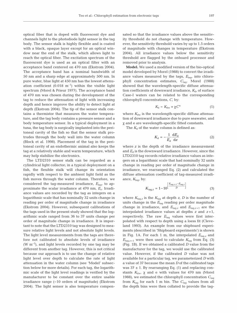
optical fiber that is doped with fluorescent dye andchannels light to the photodiode light sensor in the tagbody. The sensor stalk is highly flexible and is coatedwith a black, opaque layer except for an optical win-dow near the end of the stalk, which allows light toreach the optical fiber. The excitation spectrum of thefluorescent dye is used as an optical filter with anacceptance band centered on 470 nm (Ekstrom 2004).The acceptance band has a nominal bandwidth of50 nm and a sharp edge at approximately 500 nm. Inpure water, blue light at 450 nm has the lowest attenu-ation coefficient (0.018 m–1) within the visible lightspectrum (Morel & Prieur 1977). The acceptance bandof 470 nm was chosen during the development of thetag to reduce the attenuation of light with increasingdepth and hence improve the ability to detect light atdepth (Ekstrom 2004). The tip of the sensor stalk con-tains a thermistor that measures the water tempera-ture, and the tag body contains a pressure sensor and abody temperature sensor. In a typical deployment in atuna, the tag body is surgically implanted into the peri-toneal cavity of the fish so that the sensor stalk pro-trudes through the body wall into the water column(Block et al. 1998). Placement of the tag in the peri-toneal cavity of an endothermic animal also keeps thetag at a relatively stable and warm temperature, whichmay help stabilize the electronics.

The LTD2310 sensor stalk can be regarded as acylindrical light collector; in a typical deployment on afish, the flexible stalk will change its orientationrapidly with respect to the ambient light field as thefish moves through the water column. Therefore, weconsidered the tag-measured irradiance, Etag, to ap-proximate the scalar irradiance at 470 nm, Eo. Irradi-ance values are recorded by the tag as integers on alogarithmic scale that has nominally 32 units change inreading per order of magnitude change in irradiance(Ekstrom 2004). However, subsequent calibrations ofthe tags used in the present study showed that the log-arithmic scale ranged from 36 to 37 units change perorder of magnitude change in irradiance. It is impor-tant to note that the LTD2310 tag was designed to mea-sure relative light levels and not absolute light levels.The light level measurements from the tags are there-fore not calibrated to absolute levels of irradiance(W m–2), and light levels recorded by one tag may bedifferent from another tag. However, this is not criticalbecause our approach is to use the change of relativelight level over depth to calculate the rate of lightattenuation in the water column (see ‘Model’ subsec-tion below for more details). For each tag, the logarith-mic scale of the light level readings is verified by themanufacturer to be constant over the entire usableirradiance range (~10 orders of magnitude) (Ekstrom2004). The light sensor is also temperature compen-

sated so that the irradiance values above the sensitiv-ity threshold do not change with temperature. How-ever, the sensitivity threshold varies by up to 1.5 ordersof magnitude with changes in temperature (Ekstrom2004). All irradiance values below the sensitivitythreshold are flagged by the onboard processor andremoved prior to analysis.

Model. We used a modified version of the bio-opticalmodel developed by Morel (1988) to convert the irradi-ance values measured by the tags, Etag, into chloro-phyll concentration estimates, Ctag. Morel (1988)showed that the wavelength-specific diffuse attenua-tion coefficients of downward irradiance, Kd, of surfaceCase-I waters can be related to the correspondingchlorophyll concentrations, C, by:

Kd ≈ Kdw + χCe (1)

where Kdw is the wavelength-specific diffuse attenua-tion of downward irradiance due to pure seawater, andχ and e are wavelength-specific fitted constants.

The Kd of the water column is defined as:

(2)

where z is the depth of the irradiance measurementand Ed is the downward irradiance. However, since theLTD2310 tag records relative irradiance values as inte-gers on a logarithmic scale that had nominally 32 unitschange in reading per order of magnitude change inirradiance, we rearranged Eq. (2) and calculated thediffuse attenuation coefficient of tag-measured irradi-ance, Ktag, by:

(3)

where Ktag,z is the Ktag at depth z, D is the number ofunits change in the Etag reading per order magnitudechange in irradiance, and Etag,z and Etag,z +1 are theinterpolated irradiance values at depths z and z +1,respectively. The raw Etag values were first inter-polated with respect to depth using a loess fit (Cleve-land 1993). An example from our shipboard experi-ments (described in ‘Shipboard experiments’) is shownin Fig. 1A. For each 1 m, the interpolated Etag,z andEtag,z +1 were then used to calculate Ktag from Eq. (3)(Fig. 1B). If we obtained a calibrated D value from themanufacturer for the tag, we would use the calibratedvalue. However, if the calibrated D value was notavailable for a particular tag, we parameterized D witha value of 37 because the mean D of the calibrated tagswas 37 ± 1. By rearranging Eq. (1) and replacing con-stants Kdw, χ and e with values for 470 nm (Morel1988), we estimated the chlorophyll concentration Ctag

from Ktag for each 1 m bin. The Ctag values from allthe depth bins were then collated to provide the tag-

K z

E E

D

z z

tag,

tag, tag,

= −+ −⎡

⎣⎢⎤⎦⎥1 10

1

KE

Ezd

d

ddd

= − 1

197

Aquat Biol 5: 195–207, 2009

estimated chlorophyll profile (Fig. 1C). This model wascoded in Matlab (Matlab R14SP3, Mathworks).

Although the tag measures scalar irradiance ratherthan downward irradiance, computer simulationsshow that Kd is well approximated by the diffuse atten-uation coefficient of scalar irradiance, Ko (Ko/Kd = 1.01to 1.06), for natural values of scattering and ab-sorbance in the water column (Kirk 1994). Therefore,we expect to overestimate the chlorophyll concentra-tion by up to 6% due to our use of scalar rather thandownward irradiance. However, this source of errorwould not change the shape of the profile substantiallybecause it affects the estimates equally. We considerthis level of error to be acceptable because our aimin this study is to demonstrate the feasibility of thisapproach and approximate the relative chlorophyllprofile to the first-order. With further improvements tothis approach, we believe that the errors can and willbe reduced substantially. We detail the likely sourcesof error and their effects in the discussion

Shipboard experiments. In 2003 and 2005, weassessed the ability of LTD2310 tags to estimate chloro-phyll concentrations during oceanographic cruises onthe SSV ‘Robert C. Seamans’. Each cruise consisted ofa roundtrip between Oahu, Hawaii, and Palmyra Atoll,with 7 oceanographic stations (Fig. 2). At each station,we attached 2 LTD2310 tags (programmed to recordevery 4 s) to the top of the water-sampling carousel(SBE 32-16, Seabird Electronics), with the sensor stalkprotruding into the water column. During a typicaldeployment on a pelagic fish, the sensor stalk pro-trudes into the water column from the side of the fish.The orientation of the sensor stalk on the carouselapproximated the orientation during a typical deploy-ment on a fish. Our aim for this set of experiments wasto assess our approach under relatively controlled con-ditions with fewer changes in optical orientation thanwould be expected for the deployments on pelagic fish(see ’Materials and Methods — Pacific bluefin tuna ex-periments’). The carousel was equipped with 12 2.5 lNiskin bottles (General Oceanics) and an SBE-19plusCTD profiler (Seabird Electronics) with an attached insitu chlorophyll fluorometer (SCF, Seapoint Sensors).Oceanographic sampling was conducted at approxi-mately local noon and had maximum depths of 534 ±50 m (Table 1).

After each cast, the light attenuation (Ktag) andchlorophyll concentration (Ctag) estimates for each tagwere calculated using the method described above,and vertical profiles were constructed from these val-ues. The Ctag profiles in the euphotic zone for each sta-tion were compared to the chlorophyll profiles from thefluorometer and the water samples taken using theNiskin bottles. We only compared chlorophyll profilesin the euphotic zone because all chlorophyll maxima

198

0

40

80

120

160

200320 340 360 380 400 420 440

Tag-measured irradiance, Etag (tag units)

Dep

th (m

)

A

0

40

80

120

160

200

Dep

th (m

)

16 18 20 22 24 26 28

1.5 2.0 2.5 3.5 4.53.0 4.0 5.0

Diffuse attenuation coefficient, Ktag (x10–2 m–1)

Water temperature (°C)

B

0 0.05 0.10 0.15 0.250.20

0

40

80

120

160

200

Dep

th (m

)

Chlorophyll concentration (mg m–3)

C

Fig. 1. Irradiance, diffuse attenuation coefficient and chloro-phyll profiles from the upper 200 m at Stn S187-045 in 2003,using tag A0586. (A) Irradiance (Etag) measured by tag A0586(grey circles) and interpolated irradiance profile calculatedusing a loess fit (solid line). (B) Water temperature profile(dotted line) and the diffuse attenuation coefficient profileof tag-measured irradiance, Ktag (black line), which wascalculated from the interpolated irradiance profile. (C) Tag-

estimated chlorophyll profile, using Eq. (1)

Teo et al.: Chlorophyll estimation from electronic tags

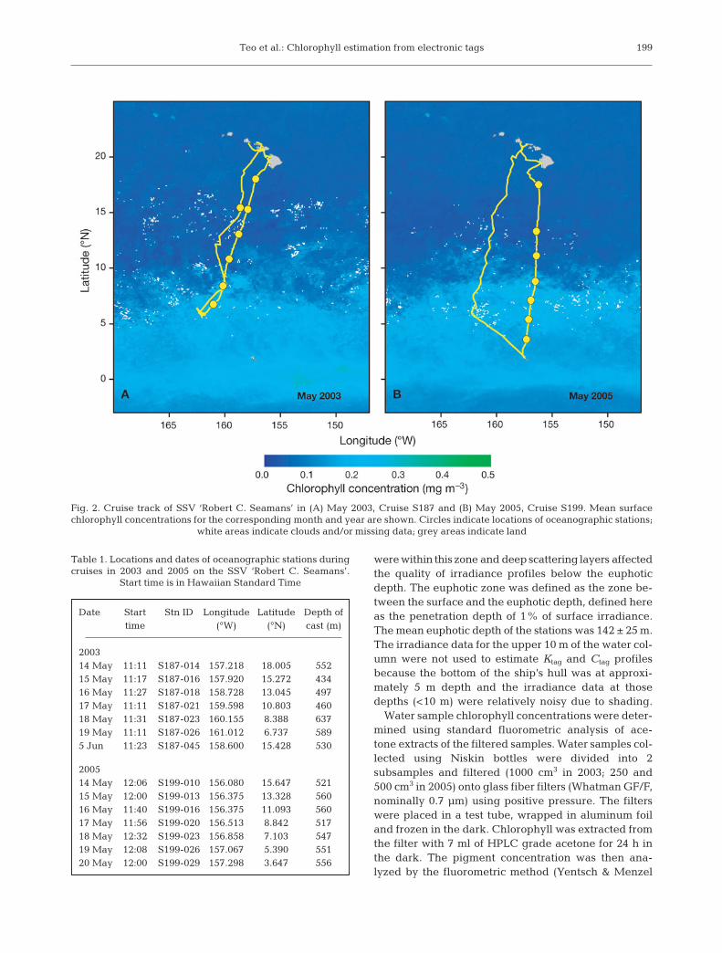
were within this zone and deep scattering layers affectedthe quality of irradiance profiles below the euphoticdepth. The euphotic zone was defined as the zone be-tween the surface and the euphotic depth, defined hereas the penetration depth of 1% of surface irradiance.The mean euphotic depth of the stations was 142 ± 25 m.The irradiance data for the upper 10 m of the water col-umn were not used to estimate Ktag and Ctag profilesbecause the bottom of the ship’s hull was at approxi-mately 5 m depth and the irradiance data at thosedepths (<10 m) were relatively noisy due to shading.

Water sample chlorophyll concentrations were deter-mined using standard fluorometric analysis of ace-tone extracts of the filtered samples. Water samples col-lected using Niskin bottles were divided into 2subsamples and filtered (1000 cm3 in 2003; 250 and500 cm3 in 2005) onto glass fiber filters (Whatman GF/F,nominally 0.7 µm) using positive pressure. The filterswere placed in a test tube, wrapped in aluminum foiland frozen in the dark. Chlorophyll was extracted fromthe filter with 7 ml of HPLC grade acetone for 24 h inthe dark. The pigment concentration was then ana-lyzed by the fluorometric method (Yentsch & Menzel

199

Fig. 2. Cruise track of SSV ‘Robert C. Seamans’ in (A) May 2003, Cruise S187 and (B) May 2005, Cruise S199. Mean surfacechlorophyll concentrations for the corresponding month and year are shown. Circles indicate locations of oceanographic stations;

white areas indicate clouds and/or missing data; grey areas indicate land

Table 1. Locations and dates of oceanographic stations duringcruises in 2003 and 2005 on the SSV ‘Robert C. Seamans’.

Start time is in Hawaiian Standard Time

Date Start Stn ID Longitude Latitude Depth of time (°W) (°N) cast (m)

200314 May 11:11 S187-014 157.218 18.005 55215 May 11:17 S187-016 157.920 15.272 43416 May 11:27 S187-018 158.728 13.045 49717 May 11:11 S187-021 159.598 10.803 46018 May 11:31 S187-023 160.155 8.388 63719 May 11:11 S187-026 161.012 6.737 5895 Jun 11:23 S187-045 158.600 15.428 530

200514 May 12:06 S199-010 156.080 15.647 52115 May 12:00 S199-013 156.375 13.328 56016 May 11:40 S199-016 156.375 11.093 56017 May 11:56 S199-020 156.513 8.842 51718 May 12:32 S199-023 156.858 7.103 54719 May 12:08 S199-026 157.067 5.390 55120 May 12:00 S199-029 157.298 3.647 556

Aquat Biol 5: 195–207, 2009

1963) with a blanked and calibrated fluorometer(Turner Designs 10-AU). For each station and depth, wecalculated the mean chlorophyll concentration from the2 subsamples and compared that to corresponding Ctag

profiles. The Ctag profiles were also compared withthose made by the in situ chlorophyll fluorometer (Ast-heimer & Haardt 1984). We correlated the Ctag profileswith the chlorophyll concentrations from the watersamples and the fluorometer and calculated the overallrms difference between the corresponding profiles.The rms differences in the chlorophyll maxima depthsdetected by the 3 methods were also calculated.

In addition, we used the ADCP (75 kHz Ocean Sur-veyor, RD Instruments) aboard the vessel to estimatethe deep scattering layer depth and compared theADCP’s echo intensity profile with the Ktag profile atthe oceanographic stations. The acoustic backscatterstrength of the water column is related to the biomassprofile of the water column and the ADCP’s echo inten-sity profile has been used to estimate the biomass ofdeep scattering layers (Flagg & Smith 1989, Heywoodet al. 1991, Griffiths & Diaz 1996). Since light attenua-tion also increases with increased biomass in the watercolumn, we hypothesized that the light attenuationprofiles from the tags may be comparable to the echointensity profiles from the shipboard ADCP. We set theADCP software to aggregate the raw echo intensity ofeach acoustic beam into ensembles of 20 min and 10 mbins (60 bins, 18 to 608 m). The echo intensity profilesof the 4 beams were then averaged to obtain the echointensity profile of each ensemble. For each station, weselected the echo intensity profiles from 3 ensemblescollected during the cast and compared the mean echointensity profile with Ktag profiles obtained by the tag.The deep scattering layer depth of each station wasdetermined by the depth of the secondary peak of theecho intensity profile. We then calculated the rmsdifference between the deep scattering layer depthsestimated by the ADCP and the tag.

Pacific bluefin tuna experiments. We also assessedthis method by deploying 48 LTD2310 archival tags onPacific bluefin tuna in the eastern tropical PacificOcean. The fish were caught by commercial purseseines and transferred by tow pens to grow-out penson the Pacific coast of Baja California, Mexico. On9 March 2005, the fish were brought up onto a vinylsurgical pad on the deck of a barge for surgery. Eachbluefin tuna was measured (cm curved fork length[CFL]) and an LTD2310 archival tag was surgicallyimplanted into the peritoneal cavity of the fish so thatthe sensor stalk protruded from the body of the fish(Block et al. 1998). The fish were immediately trans-ferred to a tow pen that was towed offshore (31.718° N,116.997° W) before the fish were released. All proce-dures were conducted in accordance with approved

animal care protocols. The tags were programmed tosample every 4 or 8 s. Since the LTD2310 tags weresurgically implanted into the peritoneal cavity of thetuna, the fish had to be recaptured to retrieve the tagand the collected data.

Sixteen of the tagged bluefin tuna were subsequentlyrecaptured by commercial fishers. For each day, we ex-tracted the irradiance and pressure data from a periodof 2 h surrounding the local noon to minimize variationof the ambient light field (see ‘Discussion’ for more de-tails). Corresponding Ctag values were estimated fromthe extracted irradiance and depth data using themethod described above. Irradiance data from the up-per 10 m were not used because the irradiance data atthose depths were relatively noisy. Profiles with sparsedata (<100 data points) or large spikes (>2.0 mg m–3)were eliminated before further analysis. Based on theWOD (www.nodc.noaa.gov) and our oceanographiccasts in the area, this value is outside the 95% confi-dence interval of subsurface chlorophyll maxima con-centrations recorded in the area. Individual chlorophyllprofiles were smoothed with a robust, locally weightedleast squares fit (Cleveland 1993). To visualize how thechlorophyll profiles from a single fish changed overtime, we concatenated daily Ctag profiles from the samefish into a single array and applied a 2-dimensional 3 ×3 median filter to reduce noise in the array.

Geolocations of the Pacific bluefin tuna were esti-mated from light level longitude and sea surface tem-perature (SST) data recorded by the tags using a mod-ification of the methods described by Teo et al. (2004).SST data from the tags were combined with corre-sponding light level longitude estimates to obtain dailylatitude estimates. For a given day, the latitude atwhich the tag-recorded SSTs best matched the corre-sponding remotely sensed SSTs, along the light levellongitude estimate, was considered the latitude esti-mate for the day. Based on swimming speeds estimatedfrom acoustic tracking studies (Boustany et al. 2001),the SST matching process for each day was con-strained to the area that the fish could have realisti-cally moved. We also improved the geolocation algo-rithm with the addition of the capacity to switch tocloud-free, microwave-based, remotely sensed SST data(TMI/AMSRE, ftp:/ftp.discover-earth.org/sst/) duringperiods with high cloud cover, and an improvement tothe algorithm used ensured the movement path did notcross land. Daily maximum diving depths recorded bythe tags were also used to filter geolocation estimatesso that the maximum diving depth did not exceed theknown bathymetry (inclusive of error estimates) atthe geolocation estimate for the corresponding day.Archival tags were found to have rms errors of 0.78°and 0.90° for longitude and latitude estimates, respec-tively (Teo et al. 2004).

200

Teo et al.: Chlorophyll estimation from electronic tags

Mean depths of the chlorophyll maxima and meanchlorophyll concentrations at the maxima estimatedfrom electronic tags were compared to the profilesrecorded in the WOD for the season and region. Here,we used Ctag profiles that went deeper than theeuphotic depth to ensure that the profiles includedthe chlorophyll maxima. We extracted correspondingWOD chlorophyll profiles for the same month thatwere within 1° of the geolocation estimate. However,the WOD profiles were typically from a different year.It was therefore not possible to determine the actualerrors in the tag-derived chlorophyll estimates be-cause the chlorophyll data from the WOD were from adifferent year and therefore not the actual chlorophyllconcentration when the bluefin tuna was in the area.However, this was not critical because we did not setout to determine the error distribution of the chloro-phyll estimates. Rather, our aim for this set of experi-ments was to determine if we could derive reasonablechlorophyll profiles for this area and season usingthese electronic tags. We assumed that the chloro-phyll profiles in the WOD for the same season andregion provided a reasonable range of chlorophyllmaxima concentrations and depth likely to be experi-enced by the tuna. We subsequently calculated theoverall rms differences between the chlorophyllmaxima concentrations and depths from the tags andthe WOD. In addition, we determined if the chloro-phyll maxima concentration and depth of each profilewere within the 95% confidence interval of the corre-sponding WOD mean chlorophyll maxima concentra-tion and depth.

RESULTS

Shipboard experiments

In the euphotic zone, chlorophyll profiles estimatedby the LTD2310 tags were representative of theoceanographic stations and were similar to the profilesmeasured from the fluorometer and water samples. Asan example, the chlorophyll concentrations deter-mined by all 3 methods at Stn S187-045 are shown inFig. 3. Across all 14 stations, tag-estimated chlorophyllconcentrations were significantly correlated withchlorophyll concentrations measured from the fluoro-meter (R2 = 0.29, n = 142, p < 0.0001) and water sam-ples (R2 = 0.41, n = 142, p < 0.0001) (Fig. 4). However,there were clearly differences between the methods.Overall rms differences between the euphotic zonechlorophyll concentrations estimated by the tag versuscorresponding chlorophyll concentrations measuredfrom the filtered water samples and fluorometer were0.088 and 0.27 mg m–3 (n = 142), respectively. This

201

0 0.05 0.10 0.15 0.250.20

0

40

80

120

160

200

Dep

th (m

)

Chlorophyll concentration (mg m–3)

Fig. 3. Chlorophyll profiles from the upper 200 m at Stn S187-045, using tag A0586 (––––), filtered water samples (------)

and profiling fluorometer (– – – –)

A0.7

0.6

0.5

0.4

0.3

0.2

0.1

00 0.05 0.10 0.15 0.20 0.30 0.400.25 0.35

Water sample chlorophyll concentration (mg m–3)

Tag

-estim

ate

d c

hlo

rop

hyll

co

ncentr

atio

n (m

g m

–3)

B0.7

0.6

0.5

0.4

0.3

0.2

0.1

00 0.2 0.4 0.6 0.8 1.0 1.2 1.4

Fluorometer chlorophyll concentration (mg m–3)

R2 = 0.29p < 0.0001N = 142

R2 = 0.41p < 0.0001N = 142

Fig. 4. Correlation of tag-estimated chlorophyll concentra-tions with (A) filtered water samples and (B) profiling fluoro-

meter from all oceanographic stations

Aquat Biol 5: 195–207, 2009

compares well with the rms difference (0.23 mg m–3,n = 142) between corresponding chlorophyll concen-trations measured from the filtered water samples andthe fluorometer.

This method performed well overall during bothcruises but it performed relatively poorly at one stationduring each cruise (S187-026 and S199-023). At bothstations, the Ctag profiles did not match the profilesmeasured from the water samples. Interestingly, bothstations were at approximately the same latitude (7°N)(Table 1), which was at the edge of the equatorial up-welling zone, and both stations had relatively shallowchlorophyll maxima.

Below the euphotic zone, the deep scattering layersinfluenced the Ktag profile. The Ktag profiles showed alarge secondary peak below the euphotic zone eventhough there is only a negligible amount of chlorophyllat those depths (Fig. 5). These deeper peaks corre-sponded well to the depths at which the ADCP echointensity increased (Fig. 5). The increased echo inten-sity indicates the presence of deep scattering layersand increased biomass at those depths (Flagg & Smith1989, Heywood et al. 1991). Based on the ADCP, thedeep scattering layers during the oceanographic sta-

tions were at depths ranging from approximately 290to 440 m. The overall rms difference between the deepscattering layer depths estimated by the tags and theADCP was 17 m.

Pacific bluefin tuna experiments

For the Pacific bluefin tuna experiments, tag-esti-mated chlorophyll profiles were comparable to chloro-phyll profiles recorded in the WOD for the region. Asan example, the irradiance profile collected bybluefin tuna C0071 from 2 June 2005 was used toestimate the Ktag and Ctag profiles (Fig. 6A). The Ctag

profile was comparable to the WOD chlorophyll pro-files in June that were within 1° of the fish’s geoloca-tion (Fig. 6B).

Overall, chlorophyll profiles from the bluefin tunahad maximal chlorophyll concentrations and chloro-phyll maxima depths that were similar to thoserecorded in the WOD for the Baja California region.The rms differences between the Ctag at the chloro-phyll maxima and the WOD chlorophyll profiles were0.23 and 0.26 mg m–3 for tags sampling at every 4and 8 s, respectively. Most of the tag-estimated max-imal chlorophyll concentrations (91.8% for 4 s tags,88.5% for 8 s tags) were also within the 95% confi-dence intervals of the WOD maximal chlorophyllconcentrations. In addition, the rms differences inthe chlorophyll maxima depths estimated by the tagsand in the WOD were 25 and 26 m for the tags sam-pling at 4 and 8 s, respectively. The majority of tag-estimated chlorophyll maxima depths (82.4% for 4 stags, 73.0% for 8 s tags) were also within the 95%confidence intervals of the WOD chlorophyll maximadepths.

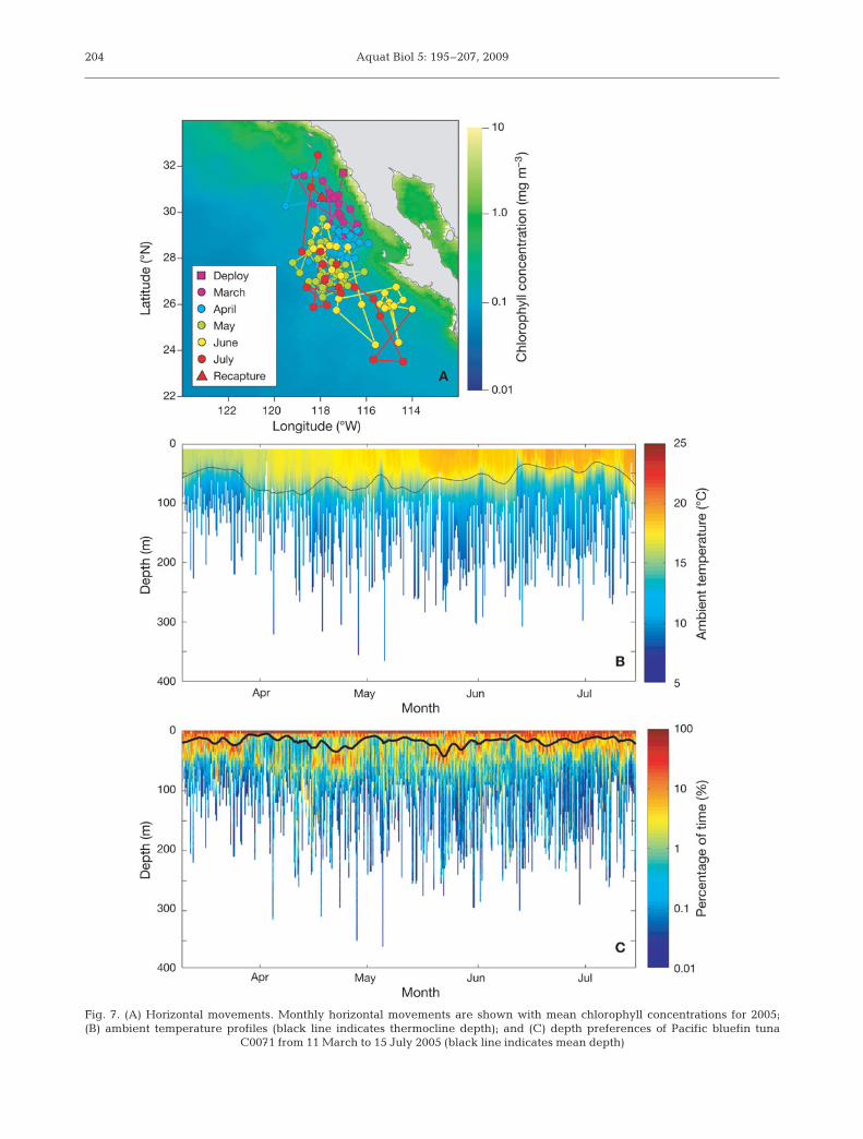
Daily chlorophyll profiles were concatenated to illus-trate the changes in their chlorophyll profiles (seeFig. 6C for an example for bluefin tuna C0071). Forinstance, the mean chlorophyll concentration at thechlorophyll maxima for bluefin tuna C0071 was 0.45 ±0.08 mg m–3 and the mean chlorophyll maxima depthwas 69 ± 14 m. Changes in the Ctag profiles were com-pared to the corresponding horizontal movements,ambient temperature profiles and depth preferences(Fig. 7); however, a detailed analysis of this is beyondthe scope of this paper. Depths of the chlorophyllmaxima from bluefin tuna C0071 were significantlycorrelated with the thermocline depth (R2 = 0.60, p <0.0001). The correlation between the thermocline andthe chlorophyll maxima depths adds to our confidencein the Ctag profiles because the nutricline is closelyrelated to the thermocline in the region and the chloro-phyll profile is likely to be related to the nutriclinedepth (Wilson & Coles 2005).

202

Fluorometer chlorophyll concentration (mg m–3)

Dep

th (m

)

0

100

200

300

400

500

0 1 2 3 4 5 6 7 8

20 40 60 80 100 120 140 160

ADCP echo intensity (counts)

0 0.05 0.15 0.25 0.35 0.10 0.20 0.30

Diffuse attenuation coefficient, Ktag (x10–2 m–1)

Fig. 5. Profiles of diffuse attenuation coefficients, Ktag, esti-mated from tag C0300 (––––), chlorophyll concentrations esti-mated by the fluorometer (– – – –) and Acoustic Doppler Cur-rent Profiler (ADCP) echo intensity (------) at Stn S199-010.Arrows indicate peaks of Ktag at this station, with the shallowpeak coinciding with the chlorophyll maxima and the deep

peak coinciding with a peak in ADCP echo intensity

Teo et al.: Chlorophyll estimation from electronic tags

DISCUSSION

In the present study, we have demonstrated the con-cept of using light level and depth data from geo-locating electronic tags deployed on pelagic animals toobtain in situ chlorophyll profiles. Although thereclearly remains much more work to be done to improvethe accuracy and precision of the chlorophyll esti-mates, our results suggest that the approach is promis-ing. With further refinements to this approach, re-search programs utilizing electronic tags can maximizethe use of oceanographic data collected by these tags.One potential use will be to obtain subsurface chloro-phyll profiles along an animal’s path while simultane-ously observing the animal’s behavior and physiology,which will likely improve our understanding of the

relationship between pelagic animals and the deepchlorophyll maxima. In addition, it also has the poten-tial to greatly increase the number of in situ chloro-phyll profiles available to the oceanographic com-munity and, hence, improve our understanding ofsubsurface chlorophyll dynamics.

One of the important sources of error is variability inthe ambient light field. If the ambient light field israpidly changing, any change in the irradiance profilemight reflect ambient light field changes rather thanlight attenuation. To reduce the influence of ambientlight field variability, we only used data from a 2 hperiod around the local noon, which improves theaccuracy and reduces the variability of the Ktag and,hence, the Ctag profiles. Since the rate of change ofsolar irradiance is at its slowest during local noon, this

203

Fig. 6. Irradiance, ambient temperature and chlorophyll profiles estimated from Pacific bluefin tuna C0071 on 2 June 2005 offBaja California. (A) Irradiance (Etag, grey circles) and interpolated irradiance profile calculated using a loess fit (red line).(B) Chlorophyll profiles estimated from the tag (green) and in the World Ocean Database for the month of June and within 1° ofthe fish’s estimated geolocation for 2 June 2005 (dashed lines). (C) Chlorophyll profiles of Pacific bluefin tuna C0071 from

11 March to 15 July 2005. Black line indicates depth of chlorophyll maxima

Aquat Biol 5: 195–207, 2009204

Fig. 7. (A) Horizontal movements. Monthly horizontal movements are shown with mean chlorophyll concentrations for 2005;(B) ambient temperature profiles (black line indicates thermocline depth); and (C) depth preferences of Pacific bluefin tuna

C0071 from 11 March to 15 July 2005 (black line indicates mean depth)

Teo et al.: Chlorophyll estimation from electronic tags

would reduce ambient light field changes and henceimprove the Ktag and Ctag profiles. The high solar ele-vation angle during local noon also reduces the effectof changing atmospheric conditions because the ap-parent atmospheric optical thickness is reduced. Inaddition, the high solar elevation angle reduces thereflectance and diffraction of light at the air–sea inter-face due to Snell’s law and the irradiance profile in thewater is less influenced by a changing sea state (Kirk1994). Another advantage is that the solar irradiance,for a given day and set of conditions, is maximal duringlocal noon, which would increase the penetrationdepth of light and hence the depth range for which thismethod is effective.

Diving behavior of the animal also interacts with thetag’s optical geometry to affect our ability to estimatechlorophyll profiles. Here, we used the LTD2310 tag,which has a flexible cylindrical light collector thatprotrudes into the water column and moves aroundrapidly as the animal swims. Hence, the tag can beassumed to measure overall scalar irradiance (i.e. mea-suring light equally from all directions). Therefore, theangle at which the photons intercept the light sensordoes not affect the tag’s irradiance measurement. Onthe other hand, cosine collectors (flat light sensors thatface upwards or downwards) are sensitive to the angleat which the photons intercept the light collector.Therefore, tags with cosine collectors are more likelyto be sensitive to changes in the tag’s orientation dur-ing an animal’s dive. If the orientation of the animalduring a dive is relatively random, changes in the opti-cal geometry should equal out over time. However, ifthe animal’s orientation changes in a regular fashionduring specific parts of the dive, it would be importantto correct the irradiance data for body orientation.

For this method to be effective when the pelagicanimals are moving rapidly over large spatial scales atrelatively short temporal scales, it will likely requiremodifications to the algorithm described here. Whenpelagic animals are moving rapidly, the animal may bemoving through several water masses within a shorttime period. Therefore, the light attenuation profiledata from a single day may consist of a mixture of lightattenuation profiles from different water masses. Onepossible way to tackle this problem would be to focusthe analysis on an individual dive over a short timeperiod. In this way, the chance of the data being frommultiple water masses is reduced. The drawback ofthis approach, however, is that the tag would need tobe sampling at very high rates for there to be enoughlight and depth data for analysis.

The relatively poor performance of this method atthe oceanographic stations close to the upwelling zonesuggests the need for potential improvements to thecurrent method. In addition to increased primary pro-

ductivity, upwelling zones also tend to have increasedsecondary productivity, especially near the edges ofthe upwelling zones (Cury & Roy 1989). The increasedzooplankton abundance in upwelling areas may haveled to a reduction in the performance of Morel’s (1988)bio-optical model, which was parameterized for Case-I(open ocean) waters. One way to improve the futureperformance of this method is to measure the irradi-ance and attenuation at multiple optical bands, ratherthan a single optical band. For example, the ratiobetween the remote sensing reflectance at 490 and555 nm is used in empirical and semianalytic bio-optical models to estimate the surface chlorophyllcontent from remote sensing data (O’Reilly et al. 1998).Since the remote sensing reflectance at a specificwavelength is related to Kd (Mobley 1994), we will beable to use a similar multi-band approach to estimatechlorophyll profiles from electronic tags. Indeed, weare currently testing the use of dual-band tags onnorthern elephant seals to estimate chlorophyll pro-files. These multi-band instruments will also allow usto use new bio-optical algorithms developed for pas-sive optical sensors deployed on AUVs and Argo floats(Brown et al. 2004).

Besides Morel (1988), there are alternative bio-opticalmodels that can be used with electronic tags and itwould be useful to compare the performance of thesedifferent models in future studies. However, it wouldbe important that the details of each model be under-stood and found to be applicable for the study. Forexample, Morel & Maritorena (2001) used new opticaldata from several Joint Global Ocean Flux Study(JGOFS) cruises to revise Morel’s (1988) bio-opticalmodel. However, we were unable to use those resultsin the present study because the in situ chlorophyllconcentrations from the JGOFS cruises were primarilymeasured using HPLC (Morel & Maritorena 2001). Incontrast, the chlorophyll concentration data fromMorel (1988) were primarily determined using fluoro-metric methods, which were similar to the methodsused in the present study. In addition, it would be use-ful to compare the performance of electronic tags fromdifferent manufacturers under different environmentalconditions. Since the optics and electronics of tagsfrom different manufacturers can differ substantially,we expect that this may result in differing abilities toestimate chlorophyll concentrations.

Bio-optical models are typically developed for sur-face waters, but we showed that Ktag profiles below theeuphotic zone might be used to estimate deep scatter-ing layer depths. The Ktag profiles often showed a largesecondary peak below the euphotic zone even thoughthere was only a minimal amount of chlorophyll atthose depths. These deeper peaks corresponded tothe depths at which ADCP echo intensity increased

205

Aquat Biol 5: 195–207, 2009

(Fig. 5), suggesting that scattering and absorbance oflight by animals in the deep scattering layers weredetected by the tags. However, caution should be usedin interpreting this result because the irradiance levelsat these depths were approaching the detection limit ofthis generation of tags. We speculate that the next gen-eration of tags, with potentially 2 to 3 more orders ofmagnitude of sensitivity to light, might be used to vali-date the ability to estimate deep scattering layerdepths. In addition, it would be important to test this bydeploying tags on species that are associated with thedeep scattering layer and dive repeatedly through thewater column during the day, e.g. bigeye tuna and ele-phant seals (Dagorn et al. 2000, Le Boeuf et al. 2000,Campagna et al. 2001, Schaefer & Fuller 2002). In thefuture, it would also be interesting to correlate the bio-mass at these depths with the Ktag profiles obtainedfrom the tags. This would enable us to estimate thedeep scattering layer biomass with these tags andallow us to determine if long-term changes in divingbehavior are related to changes in the deep scatteringlayer depth and biomass. Currently, we have to deployships or AUVs to obtain acoustic profiles or net sam-ples of the deep scattering layer at the same time as theanimal is being tracked (Dagorn et al. 2000).

Acknowledgements. We thank all participants of the work-shops organized by the Tagging of Pacific Pelagics (TOPP)project, especially S. Simmons, for discussions that led to thisstudy, as well as the captain, crew, instructors and students ofthe Stanford@SEA classes on the SSV ‘Robert C. Seamans’ fortheir enthusiasm and assistance in data collection. We partic-ularly thank J. Witting, K. Lavendar and R. Dunbar for theirhelp on these cruises. We would also like to thank members ofthe Block Lab for helping us tag bluefin tuna in Baja Califor-nia, especially C. Farwell and T. Williams. Five anonymousreviewers provided comments that improved the manuscript.Funding was provided by the David and Lucile Packard,Alfred P. Sloan and Gordon and Betty Moore Foundations.

LITERATURE CITED

Astheimer H, Haardt H (1984) Small-scale patchiness of thechlorophyll fluorescence in the sea: aspects of instrumen-tation, data processing, and interpretation. Mar Ecol ProgSer 15:233–245

Baumgartner MF, Cole TVN, Campbell RG, Teegarden GJ,Durbin EG (2003) Associations between North Atlanticright whales and their prey, Calanus finmarchicus, overdiel and tidal time scales. Mar Ecol Prog Ser 264:155–166

Behrenfeld MJ, Falkowski PG (1997) Photosynthetic ratesderived from satellite-based chlorophyll concentration.Limnol Oceanogr 42:1–20

Biuw M, Boehme L, Guinet C, Hindell M and others (2007)Variations in behavior and condition of a Southern Oceantop predator in relation to in situ oceanographic condi-tions. Proc Natl Acad Sci USA 104:13705–13710

Block BA, Dewar H, Williams T, Prince ED, Farwell C, Fudge

D (1998) Archival tagging of Atlantic bluefin tuna (Thun-nus thynnus thynnus). Mar Technol Soc J 32:37–46

Block B, Costa D, Boehlert G, Kochevar R (2002) Revealingpelagic habitat use: the tagging of Pacific pelagics pro-gram. Oceanol Acta 25:255–266

Block BA, Teo SLH, Walli A, Boustany A and others (2005)Electronic tagging and population structure of Atlanticbluefin tuna. Nature 434:1121–1127

Boehlert GW, Costa DP, Crocker DE, Green P, O’Brien T,Levitus S, Le Boeuf BJ (2001) Autonomous pinnipedenvironmental samplers: using instrumented animals asoceanographic data collectors. J Atmos Ocean Technol18:1882–1893

Boustany A, Marcinek DJ, Keen JE, Dewar H, Block BA(2001) Movements and temperature preference of Atlanticbluefin tuna (Thunnus thynnus) off North Carolina: a com-parison of acoustic, archival and pop-up satellite tagging.In: Sibert JR, Nielsen JL (eds) Electronic tagging andtracking in marine fishes. Kluwer Academic Publishers,Dordrecht, p 89–108

Brown CA, Huot Y, Purcell MJ, Cullen JJ, Lewis MR (2004)Mapping coastal optical and biogeochemical variabilityusing an autonomous underwater vehicle and a new bio-optical inversion algorithm. Limnol Oceanogr Methods 2:262–281

Campagna C, Dignani J, Blackwell SB, Marin MR (2001)Detecting bioluminescence with an irradiance time-depthrecorder deployed on southern elephant seals. Mar MammSci 17:402–414

Charrassin JB, Hindell M, Rintoul SR, Roquet F and others(2008) Southern Ocean frontal structure and sea-ice for-mation rates revealed by elephant seals. Proc Natl AcadSci USA 105:11634–11639

Cleveland WS (1993) Visualizing data. Hobart Press, Summit,NJ

Costa DP, Crocker DE, Boehlert G (2002) Foraging behaviorof northern elephant seals relative to frontal features inthe North Pacific Ocean. Integr Comp Biol 42:1212–1212

Cury P, Roy C (1989) Optimal environmental window andpelagic fish recruitment success in upwelling areas. Can JFish Aquat Sci 46:670–680

Dagorn L, Bach P, Josse E (2000) Movement patterns of largebigeye tuna (Thunnus obesus) in the open ocean, deter-mined using ultrasonic telemetry. Mar Biol 136:361–371

Ekstrom PA (2004) An advance in geolocation by light. In:Naito Y (ed) Memoirs of the National Institue of PolarResearch, Special Issue, Vol 58. National Institute of PolarResearch, Tokyo, p 210–226

Fedak MA, Lovell P, Grant SM (2001) Two approaches tocompressing and interpreting time-depth information ascollected by time-depth recorders and satellite-linkeddata recorders. Mar Mamm Sci 17:94–110

Flagg CN, Smith SL (1989) On the use of the Acoustic DopplerCurrent Profiler to measure zooplankton abundance.Deep-Sea Res A 36:455–474

Griffiths G, Diaz JI (1996) Comparison of acoustic backscattermeasurements from a ship-mounted Acoustic DopplerCurrent Profiler and an EK500 scientific echo-sounder.ICES J Mar Sci 53:487–491

Heywood KJ, Scropehowe S, Barton ED (1991) Estimationof zooplankton abundance from ship-borne ADCP back-scatter. Deep-Sea Res A 38:677–691

Kirk JTO (1994) Light and photosynthesis in aquatic ecosys-tems. Cambridge University Press, Cambridge

Le Boeuf BJ, Crocker DE, Costa DP, Blackwell SB, Webb PM,Houser DS (2000) Foraging ecology of northern elephantseals. Ecol Monogr 70:353–382

206

Teo et al.: Chlorophyll estimation from electronic tags

McMahon CR, Autret E, Houghton JDR, Lovell P, Myers AE,Hays GC (2005) Animal-borne sensors successfully cap-ture the real-time thermal properties of ocean basins.Limnol Oceanogr Methods 3:392–398

Mobley CD (1994) Light and water: radiative transfer innatural waters. Academic Press, San Diego, CA

Morel A (1988) Optical modeling of the upper ocean in rela-tion to its biogenous matter content (Case-I waters).J Geophys Res C 93:10749–10768

Morel A, Maritorena S (2001) Bio-optical properties of oceanicwaters: a reappraisal. J Geophys Res C 106:7163–7180

Morel A, Prieur L (1977) Analysis of variations in ocean color.Limnol Oceanogr 22:709–722

O’Reilly JE, Maritorena S, Mitchell BG, Siegel DA and others(1998) Ocean color chlorophyll algorithms for SeaWiFS.J Geophys Res C 103:24937–24953

Polovina JJ, Balazs GH, Howell EA, Parker DM, Seki MP,Dutton PH (2004) Forage and migration habitat of logger-head (Caretta caretta) and olive ridley (Lepidochelys oli-vacea) sea turtles in the central North Pacific Ocean. FishOceanogr 13:36–51

Roe HSJ, Griffiths G (1993) Biological information from anacoustic doppler current profiler. Mar Biol 115:339–346

Roemmich D, Riser S, Davis R, Desaubies Y (2004) Autono-mous profiling floats: workhorse for broad-scale oceanobservations. Mar Technol Soc J 38:21–29

Schaefer KM, Fuller DW (2002) Movements, behavior, andhabitat selection of bigeye tuna (Thunnus obesus) in theeastern equatorial Pacific, ascertained through archivaltags. Fish Bull 100:765–788

Teo SLH, Boustany A, Blackwell S, Walli A, Weng KC, BlockBA (2004) Validation of geolocation estimates based onlight level and sea surface temperature from electronictags. Mar Ecol Prog Ser 283:81–98

Teo SLH, Boustany AM, Block BA (2007) Oceanographic pref-erences of Atlantic bluefin tuna, Thunnus thynnus, ontheir Gulf of Mexico breeding grounds. Mar Biol 152:1105–1119

Weng KC, Castilho PC, Morrissette JM, Landeira-FernandezAM and others (2005) Satellite tagging and cardiac physi-ology reveal niche expansion in salmon sharks. Science310:104–106

Wilson C, Coles VJ (2005) Global climatological relationshipsbetween satellite biological and physical observations andupper ocean properties. J Geophys Res C 110:C10001

Yentsch CS, Menzel DW (1963) A method for the determina-tion of phytoplankton chlorophyll and phaeophytin by flu-orescence. Deep-Sea Res 10:221–231

Yu XR, Dickey T, Bellingham J, Manov D, Streitlien K (2002)The application of autonomous underwater vehicles forinterdisciplinary measurements in Massachusetts andCape Cod Bays. Cont Shelf Res 22:2225–2245

207

Editorial responsibility: Hans Heinrich Janssen,Oldendorf/Luhe, Germany

Submitted: July 24, 2008; Accepted: March 19, 2009Proofs received from author(s): April 30, 2009