Estimates of the Financial Cycle for Advanced Economies

Until recently macroeconomic theory provided at most a small role for the financial system to influence the real economy. This changed with the financial crisis. Financial quantities are now believed to have real macroeconomic effects. To study these effects we need to quantify the influence of the financial system. The financial cycle, characterized by long cyclical movements in financial variables, may provide such a measure.

In this research we therefore propose a bi-variate state space model of credit and house prices that enables us to identify a single shared financial cycle. We obtain estimates of the financial cycle for a panel of 18 advanced economies.

CPB Background DocumentRob Luginbuhl, Beau Soederhuizen

en Rutger Teulings

June 2019

Estimates of the Financial Cycle forAdvanced Economies

Rob Luginbuhl & Beau Soederhuizen & Rutger Teulings �

CPB Netherlands Bureau for Economic Policy Analysis

June 3, 2019

Abstract

Until recently macroeconomic theory provided at most a small role for the �nancial

system to in uence the real economy. This changed with the collapse of Lehman Brothers

in 2008. Financial quantities such as credit and house prices are now believed to have real

macroeconomic e�ects. In order to study these e�ects we need to quantify the in uence of

the �nancial system. The �nancial cycle, characterized by long period cyclical movements

in �nancial variables, may provide such a measure. In this research we therefore propose a

bi-variate state space model of credit and house prices that enables us to identify a single

shared �nancial cycle. The �nancial cycle is modeled as an unobserved trigonometric cycle

component with a long period. We identify one shared �nancial cycle by imposing rank

reduction on the covariance matrix of the error vector driving the �nancial cycle component.

This rank reduction can be justi�ed based on a principal components argument. We obtain

estimates of the �nancial cycle for a panel of 18 advanced economies.

�Contact details. Address: Centraal Planbureau, P.O. Box 80510, 2508 GM The Hague, The Netherlands;e-mail: r.e.luginbuhl@cpb.nl, b.soederhuizen@cpb.nl, r.m.teulings@cpb.nl.We would like to thank Albert van der Horst, Bert Smid and Marente Vlekke for their valuable comments.

1 Introduction

Until recently macroeconomic theory provided at most a small role for the �nancial system to

in uence the real economy beyond the e�ects of the interest rate set by monetary authorities.

However, since the collapse of Lehman Brothers in 2008 and the Euro crisis in 2010, it has

become clear that the �nancial system has the power to greatly in uence the real economy. The

�nancial cycle might represent an important driver of the e�ect of the �nancial system on the

rest of the economy. In this research we want to determine whether we can plausibly identify a

single �nancial cycle for a panel of 18 advanced economies. In follow-up research we explore the

possibility that these �nancial cycle estimates in uence the �scal multiplier Soederhuizen et al.

(2019).

The principal stylized facts of the �nancial cycle is that it evolves in a similar fashion to the

business cycle: it cycles between persistent periods of higher and lower activity, while over the

long run the cycle has no net impact. Furthermore, the average period of the �nancial cycle is

longer than that of the business cycle, typically lasting for 15 to 20 years, while the business

cycle has a shorter average period of roughtly 7 to 10 year. We refer the reader to the recent

work of Jord�a et al. (2018), Borio (2014), Claessens et al. (2012) and Sch�uler et al. (2015) for

details.

To estimate the �nancial cycle for each country we formulate a bivariate State Space Model,

or SSM of credit and the housing price index. We based our estimates on a model of credit and

housing prices because they are generally seen as the principal series behind the �nancial cycle,

see for example de Winter et al. (2017) and R�unstler & Vlekke (2018). In our SSM we model the

�nancial cycle as an unobserved trigonometric cycle component. This cycle component e�ectively

represents a higher order autoregressive process that tends to exhibit persistent periods of down

and upturns, but has no long-run impact on the level of a series. Although in the long run

the average cycle length will be determined by an estimated parameter representing the cycle's

period, the estimated down and upturns of the cycle are time-varying, being driven by the

disturbance term of the cycle component. As a result the estimated cycle is determined by the

data.

The use of an unobserved trigonometric cycle component in SSM's to capture cyclical dy-

namics is standard in the literature, see for example Harvey (1991) and Koopman et al. (1999).

In fact, our SSM includes two unobserved trigonometric cycle components: one for the �nancial

cycle and another for the business cycle. The inclusion of two cyclical components in the context

of unobserved component time series models using Bayesian estimation techniques was earlier

proposed in Harvey et al. (2007) to better model the business cycle. In this article the authors

propose using two independently speci�ed cycles with the same period, arguing that this allows

2

the model to tend toward a band-pass �lter as discussed in Baxter & King (1999). Our model

di�ers from this research in that we specify two cyclical components each of which has its own

period: one shorter period cycle to capture the business cycle and one longer-period cycle for

the �nancial cycle.

We rely on rank reduction in our model to identify a single underlying �nancial cycle. In the

model both credit and the housing price index have their own �nancial cycles. By imposing rank

reduction on the covariance matrix of the stochastic error vector of the �nancial cycle component,

we ensure that they share a single stochastic error process. This results asymptotically in the

same �nancial cycle for both series. Our use of rank reduction to estimate a unique �nancial

cycle for a country is as far as we know new to the literature.

We justify this rank reduction based on a principal components argument: the largest eigen-

value of the unrestricted covariance matrix of the disturbance vector driving the �nancial cycle

components typically represent roughly 99% of the sum of the eigenvalues. This suggests that

the covariance of rank one is su�cient to capture the most important aspects of both cycles.

We note, however, that the rank reduction is not supported by a model test based on the Bayes

factor.

In addition to the business and �nancial cycle, our model also includes unobserved com-

ponents to capture time-varying seasonality, trends and growth rates. This results in slowly

changing underlying trends and growth rates driving the development of the series. The esti-

mated seasonal patterns and business cycles have no long-run impact on the level of the series,

as is also the case for the estimated �nancial cycle. By explicitly modeling these underlying

processes in uencing the series, we can control for their e�ects when estimating the �nancial

cycle. Note that this type of model is also referred to as an unobserved component time series

model. We refer the reader to Harvey (1991) and Durbin & Koopman (2001) for further details

on these types of models.

We perform our estimation using Bayesian methods based on Marco Chain Monte Carlo, or

MCMC simulation. A Bayesian approach has the advantage that we can include prior infor-

mation in our estimation to help identify the model. For example our priors assume that the

�nancial cycle has a longer period than the business cycle, and that the underlying growth rate

only gradually changes over time.

In the existing literature there are a number of articles in which the �nancial cycle is modeled

as an unobserved trigonometric cycle component in a SSM. In Galati et al. (2016), R�unstler &

Vlekke (2018) andWGEM (2018) the authors obtain �nancial cycle estimates for several �nancial

series. In Koopman & Lucas (2005) and de Winter et al. (2017) the authors propose SSM's with

both business and �nancial cycles modeled as unobserved trigonometric cycle components. These

articles provide cycle estimates for various European countries. Of these articles only WGEM

3

(2018) makes use of Bayesian estimation methods. The other articles all employ maximum

likelihood techniques for the estimation. Mostly importantly, however, none of the cited articles

produce estimates of an unique �nancial cycle for each country.

Our model di�ers also in other ways from those referenced above. For one, the other SSM's

are more restricted in the stochastic processes governing the trend and drift components. Sec-

ondly, we include seasonal components in our model, which allows us to base our estimates on

seasonally unadjusted data. There have been a number of articles published in which the au-

thors argue that estimates based on seasonally adjusted data are to be preferred. The problem

with seasonally adjusted data is that it tends to introduce spurious cyclicality in the data, see

for example Luginbuhl & Vos (2003), Harvey et al. (2007) and references therein.

An additional innovation involved in our estimation of the �ncancial cycle is our mixed-

frequency data set, which combines yearly data with more recent quarterly data. The annual

data represents a fourth quarter measurement, while the �rst three quarters of the year are

taken as missing. This results in a longer data set, which allows us to estimate over a sample

period containing more completed cycles. Our model-based method facilitates the estimation

with missing observation, because the estimation of SSM's with missing data is standard, see

for example Koopman et al. (1999) for details.

Finally, we note that other researcher employ �lter-based methods to estimate �nancial

cycles. For example, Jord�a et al. (2018) propose identifying �nancial cycles through the use of a

bandpass �lter using the same long-period annual data we use. Sch�uler et al. (2015) base their

estimates of the �nancial cycle for European countries via a frequency domain based approach.

Their data set begins in 1970. Rozite et al. (2016) propose a method of estimating a �nancial

cycle for the US based on principal component analysis for data from 1973 to 2014. The Bank

of International Settlements, or BIS publishes estimates of their �nancial cycle index based on

Drehmann et al. (2012). These estimates involve the use of �ltering as well as turning points.

We argue, however, that a model-based approach to the estimation of the �nancial cycle

has a number of advantages. It allows us to simultaneously account for the e�ects of changing

growth rates and seasonal patterns, and the business cycle. This model-based approach also

allows us to easily include prior information about the unobserved components in the model and

to produce model consistent forecasts both of the �nancial cycle as well as the other unobserved

components and the observed series. These bene�ts are either lacking or di�cult to realize with

�lter-based methods.

We begin by laying out our model in Section 2, after which we formulate the priors we use

in Sections 3. This will be followed by Sections 4 and 5 in which we discuss the data and the

estimation procedure. In Section 6 we present our results. We end the article in Section 7 with

a discussion of our conclusions.

4

2 The SSM speci�cation

We begin with the speci�cation of the measurement equation. The measurement equation spec-

i�es how the unobserved components and measurement error combine to produce the measured

data. Our measured data is the logarithm of the real level of the two �nancial series, which

are assumed to follow a long run trend. This trend is in turn in uenced by a growth rate that

slowly varies over time. The business cycle and �nancial cycles cause longer frequency uctua-

tions around this slowly moving trend. Therefore when the �nancial cycle is larger than zero,

�nancial market conditions are above their long-term trend. As a result the cycle components

are assumed to produce no permanent changes to the level of the series, only temporary ones.

Our model also includes seasonal factors to capture the seasonal pattern in the data.

For each country, therefore, we specify a measurement equation in which the observed data is

denoted by yit for i = 1 and 2 for the credit and house price index series, respectively, at period

t. Each of the country's series is assumed to consist of a growing trend, �it, two stationary

cyclical processes representing the business and �nancial cycles, a set of seasonal components

and a measurement error, "it. The business cycle component is denote by Bit , and the �nancial

cycle component by Fit . The seasonal components are denoted by i;j;t. This results in the

following measurement equation.

yit = �it + Fit + B

it +

[s=2]Xj=1

i;j;t + "it; ~"t � N (0;";t) (1)

Note that we adopt the notation ~"t = ("1t; "2t) here and throughout the paper. The measurement

error covariance ";t is assumed to be time-varying. This is because for most of the countries we

analyze, the earlier parts of their sample periods su�ers from a higher degree of variability due

to the fact that the initial part of their sample periods consist of yearly data of lower quality,

while the latter part of the sample periods for all countries consists of quarterly data. This leads

us to specify the measurement covariance matrix as

";t =

"�";1I (t � T �

1 ) + �h;1I (t < T �

1 ) 0

0 �";2I (t � T �

2 ) + �h;2I (t < T �

2 )

#: (2)

We denote the indicator function here by I (�), therefore the date T �

i is the date of the �rst

quarter of the sample period with the lower variance �";i for series i. In initial period is assumed

to have the higher variance �h;i. This point is discussed below in more detail in Section 4.1

1An alternative formulation could involve allowing for this type of time-varying change in the covariancematrices of the other unobserved components in the model. Experimenting with a model version in whichwe impose the time-varying structure in (2) on the trend disturbance covariance instead of the measurement

5

Values for T �

i are listed in Table B.2 in Appendix B.

The unobserved component �it in (1) represents a type of time-varying trend called a local

linear trend:

�it = �i;t�1 + �i;t�1 + �it; ~�t � N (0;�) ; � =

"��1 0

0 ��2

#(3)

Note that the covariance matrix � is restricted to be diagonal to achieve a more parsimonious

model.2 The �it is an unobserved component that represents the time-varying growth rate of

the trend. It evolves as a random walk:

�it = �i;t�1 + �it; ~�t � N (0;�) (4)

The two components of the trend �it and �it together are responsible for the slowly changing,

growing trend in the data. Together they make up what is known as a local linear trend

component.

Both unobserved components in (1) Fit and

Bit are cyclical components. In general a cyclical

component Cit (where C = F indicates a �nancial cycle, and C = B a business cycle) evolves

as follows. Cit

C�

it

!= �C

cos 2�

�Csin 2�

�C

� sin 2��C

cos 2��C

! Ci;t�1

C�

i;t�1

!+

�Cit

�C�

it

!(5)

Further we have that ~�Ct � N�0;C

�

�and ~�C�

t � N�0;C

�

�. Note that the covariance matrices

of both disturbance vectors ~�Ct and ~�C�

t are restricted to be equal. This restriction is standard,

see Harvey (1991) for details. The cycle parameter �C determines the persistence of the cycle

Cit , and �

C represents the period of the cycle.3 We note that the unobserved component C�

it

is only required for the construction of the cycle component Cit . The speci�cation is stationary

and ensures that when included in the measurement equation that the changes it induces in the

data are temporary.

We are interested in the question of whether there is a single underlying �nancial cycle.

In an attempt to answer this question, we take the approach of imposing a single underlying

�nancial cycle in our model. We achieve this by restricting the rank of the covariance matrix of

the �nancial cycle components F� to one instead of the full-rank value of two. In this manner

both of the �nancial cycles for the series in the model are assumed to be driven by the same

underlying stochastic process.

disturbance covariance makes no di�erence to the estimates we obtain for the rest of the model.2The posteriors of � tend to be small, so this restriction is of little practical signi�cance.3The period of the cycle is given by 2�=�C .

6

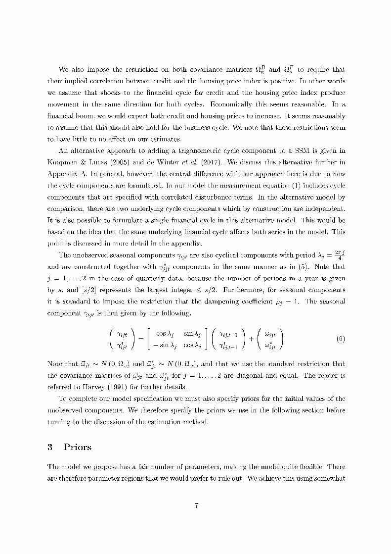
We also impose the restriction on both covariance matrices B� and F

� to require that

their implied correlation between credit and the housing price index is positive. In other words

we assume that shocks to the �nancial cycle for credit and the housing price index produce

movement in the same direction for both cycles. Economically this seems reasonable. In a

�nancial boom, we would expect both credit and housing prices to increase. It seems reasonably

to assume that this should also hold for the business cycle. We note that these restrictions seem

to have little to no a�ect on our estimates.

An alternative approach to adding a trigonometric cycle component to a SSM is given in

Koopman & Lucas (2005) and de Winter et al. (2017). We discuss this alternative further in

Appendix A. In general, however, the central di�erence with our approach here is due to how

the cycle components are formulated. In our model the measurement equation (1) includes cycle

components that are speci�ed with correlated disturbance terms. In the alternative model by

comparison, there are two underlying cycle components which by construction are independent.

It is also possible to formulate a single �nancial cycle in this alternative model. This would be

based on the idea that the same underlying �nancial cycle a�ects both series in the model. This

point is discussed in more detail in the appendix.

The unobserved seasonal components ijt are also cyclical components with period �j =2� j4

and are constructed together with �ijt components in the same manner as in (5). Note that

j = 1; : : : ; 2 in the case of quarterly data, because the number of periods in a year is given

by s, and [s=2] represents the largest integer � s=2. Furthermore, for seasonal components

it is standard to impose the restriction that the dampening coe�cient �j = 1. The seasonal

component ijt is then given by the following.

ijt

�ijt

!=

"cos�j sin�j

� sin�j cos�j

# ij;t�1

�ij;t�1

!+

!ijt

!�ijt

!(6)

Note that ~!jt � N (0;!) and ~!�

jt � N (0;!), and that we use the standard restriction that

the covariance matrices of ~!jt and ~!�jt for j = 1; : : : ; 2 are diagonal and equal. The reader is

referred to Harvey (1991) for further details.

To complete our model speci�cation we must also specify priors for the initial values of the

unobserved components. We therefore specify the priors we use in the following section before

turning to the discussion of the estimation method.

3 Priors

The model we propose has a fair number of parameters, making the model quite exible. There

are therefore parameter regions that we would prefer to rule out. We achieve this using somewhat

7

informative prior on some of the parameters. We also specify weakly informative priors to help

achieve our business and �nancial cycle decompositions with cycle periods for the business

cycle that are relatively short and for the �nancial cycle that are relatively long. For the other

parameters we specify a low prior number of degrees of freedom and select the prior scaling factor

centered around the main posterior density mass. In this way we specify fairly uninformative

empirical Bayes priors. We discuss the various prior speci�cations we use for each unobserved

component.

3.1 Cycles

Both cycle components require priors for the dampening coe�cients �C , the cycle periods �C ,

and the disturbance covariance matrices C� , for C = B and F , see (5) above. Given that the

dampening coe�cients �C 2 [0; 1), we specify a beta distribution for these priors. Note that

apriori we want �C < 1 to ensure that the cycle components are stationary and that the cycle

disturbances have no permanent e�ects on the long run level of the series. The priors for the

cycle periods �C 2 (4;1) for quarterly data, follow gamma distributions. The priors for the

covariance matrices C� are inverse Wishart distributions.

The beta priors are parameterized as Beta��Cp ; �

Cp

�, for C = B and F .4 For the business

cycle component, �B, we set �Bp = 55:88 and �Bp = 1:925. This implies a prior mean of 0:967,

with a standard deviation of 0:0234. This prior relatively di�use and has little impact on the

posteriors. The prior parameters for the �nancial cycle components' parameter �F , are give by

�Fp = 321:3 and �Bp = 4:617. These parameters imply a posterior mean of 0:986 and standard

deviation of 0:0065. Although this prior is more spread out than the posteriors, the posteriors

tend to lie slightly above the prior. This prior is therefore somewhat informative in that it tends

to pull the posterior away from the value of 1. Experimenting with di�ering prior parameters

suggests that our results are not very sensitive to this prior.

The prior gamma distribution for the �C is denoted by Gamma�aC ; bC

�, for C = B and F .5

These priors are formulated using a Bayesian highest density region, or HDR. In the case of the

business cycle, we make the prior assumption that the probability that the business cycle period

is between �ve to ten years is 99%: P�20 quarters < �B � 40 quarters

�= 99%. This results

in the prior parameter values of aB = 55:88 and bB = 4:617 for the gamma prior of �B. We

formulate our prior for the �nancial cycle period �F in a similar fashion. Here we employ the

99% prior HDR of between 15 to 20 years: P�60 quarters < �F � 80 quarters

�= 99%. This

implies the prior parameter values of aF = 321:3 and bF = 1:925 for the gamma prior of �F .

Alternative priors based on the same HDR intervals, but with lower probabilities, such as 95%

4The density function of Beta (�p; �p) is then given by f (x) = x�p�1 (1� x)�p�1 =B (�p; �p).5The density function of Gamma (a; b) is then given by f (x) = ba

�(a)xa�1 exp�b x.

8

or 90%, result in similar estimates. If, however, we increase these intervals to encompass longer

periods, then this can alter our estimates. For example an HDR for �F based on the interval

from 20 to 25 years tends to result in somewhat di�erent �nancial cycle estimates. On the

whole, however, we believe that our priors for the cycle periods represent the values most cited

in the literature, see for example Drehmann et al. (2012) and Borio (2014). Although somewhat

informative, these priors still allow the posteriors to be largely determined by the data.

We denote the prior inverse Wishart distribution for C� by W�1

��C ; SC

�, for C = B and

F .6 The prior parameter �C represents the number of degrees of freedom. For both the business

and �nancial cycle we set �B = �F = 13. Korea is an exception: in this case we use �F = 6

to ensure that the prior is weak enough to allow the likelihood to dominate the prior in the

posterior. We then select the positive (semi) de�nite matrix S to ensure that the mean of the

posterior is una�ected by the prior. These values for SC for C = B and F are listed in Table

B.1 in Appendix B.

To complete the prior speci�cation for the cycle component we also need to specify priors

for the initial values of the cycle components Ci;0 and C�

i;0 for i = 1 and 2 and C = B and

F . Provided that the dampeningen coe�cients �B < 1 and �F < 1, which given our beta

priors is the case, the cycle components' initial conditions are Ci;t � N

�0; ��Ci

=�1� �C

2��

and

C�

i;t � N�0; ��Ci

=�1� �C

2��

, when we also specify that

C� =

�C�1 �C�12

�C�12 �C�2

!(7)

for i = 1 and 2 and C = B and F .7 We also make the standard assumption that the initial

values of the cycles are uncorrelated.

3.2 Trend & Growth Rates

The two trend components �i;t in (3) and the two growth rates �i;t in (4) follow random walks.

They are therefore non-stationary. As a result we assume di�use priors for their initial values.

We discuss the use of di�use priors for the non-stationary elements of the state below in section

5.

6The density function of W�1��C ; SC

�is then given by

f (X) =jSj�=2

2��2��2

� jXj�(�+3)=2e�1

2tr(SX�1)

.7Alternatively, Harvey & Streibel (1998) argue for an alternative speci�cation where the prior variance of

Ci;0 = �C�;i, so that the variance of �Ci;t = �C�;i

�1� �C 2

�. This allows the cycle component to remain stationary,

although deterministic, as �Ci ! 1.

9

The inverse Wishart prior degrees of freedom for the disturbance covariance matrices �

for the trend component and � for the growth rate component are �� = 11 and �� = 83,

respectively. The values for the prior parameter matrices S� and S� are listed in Table B.2 of

Appendix B.

In general 11 degrees of freedom for the inverse Wishart distribution produces a prior that

is relatively uninformative. We select the values for S� to ensure that the highest prior density

region corresponds to that of the posterior.8 In this way the priors for � are selected to have

minimal impact on the form of the posteriors. This essentially an empirical Bayes approach.

Our prior speci�cation for the � are more informative. We interpret the drift components

�i;t as representing the underlying growth rates. As such we believe apriori that these rates will

only change gradually over time. It is however common in SSM's of macroeconomic time series

with a local linear trend, such as we have speci�ed here, that the likelihood tends to favor larger

values for the variance of the disturbance of the drift component. These larger values for the

variance imply a relatively quickly changing growth rate. In the case of our model we believe

that these changes ought to be captured by the cycles in the model. For this reason we specify

the larger prior parameter value of �� = 83 for � of the growth rate component. This then

represents a more informative prior. Compared with the information in the two sets of more

than 200 observations of the sample periods, this number of degrees of freedom is still fairly

modest. We specify diagonal elements of the prior parameter matrices S� which correspond to

modest changes over time in the growth rates �i;t. The o�-diagonal elements are assumed to

be zero indicating a prior of no correlation between the growth rates of credit and the housing

price index.

In those instances where the marginal posterior variance for �it was lower than our initial prior

speci�cation would suggest9, we lowered the corresponding value in S� to match the posterior. In

two instances, for the Dutch credit series and the Swedish housing price index, we adjusted the

priors to correspond to larger values of these variances to accommodate for the more dramatic

swings in these series during the Great Depression and Second World War.

3.3 Seasonal Components

The covariance matrices !1 and !2 in (6) are assumed to be diagonal. Therefore the prior

parameter matrices S!1 and S!2 are as well. In all cases we set the number of degrees of freedom

8The o�-diagonal elements of S� are zero, because � is diagonal. These priors are therefore equivalent toinverse-gamma priors with the inverse gamma distribution parameters ��i = ��=2 and ��i = s�i=2.

9We initially specify a prior on � that implies an expected value of 0.08 for both ��1 and ��2 .

10

of these inverse Wishart priors to �!1 = �!2 = 11 and

S!1 = S!2 =

"0:0002 0

0 0:0002

#: (8)

Both the credit and housing price index series exhibit only a slight degree of seasonality. We

specify di�use priors on the initial values i;j;0 and �i;j;0, because these components are non-

stationary.

3.4 Measurement Error Covariance

To specify a prior on the covariance matrix ";t of the measurement error as given in (2), we

need to specify priors on � and h where

� =

"�"1 0

0 �"2

#; h =

"�h1 0

0 �h2

#: (9)

We use inverse Wishart priors: P (�) � W�1 (��; S�) and P (h) � W�1 (�h; Sh). We can

de�ne the matrices S� and Sh as follows.

S� =

"s�1 0

0 s�2

#Sh =

"sh1 0

0 sh2

#(10)

In Table B.3 of Appendix B we list the elements of the prior parameter matrices S" and Sh.10

We also list in this table the dates T �

i when our model transitions to the lower measurement error

variance, see (2). We set the degrees of freedom �" = �h = 40, with the exception of ��2 = 4000

for Korea. The exceptional value for the Korean housing price index proved necessary to ensure

the numerical stability of the Kalman �lter in our MCMC estimation. The problem arrises due

to the presence of missing values for the Korean housing price index in the beginning of the

sample period. We discuss this point below in section 5 on the estimation of our model. First,

however, we discuss the data.

4 The data

Our sample consists of credit data and housing price indices for 18 advanced economies: Aus-

tralia, Belgium, Canada, Denmark, Finland, France, Germany, Ireland, Italy, Japan, the Nether-

10Given that the measurement errors between the two series are uncorrelated, these priors are equivalent toinverse-gamma priors on �"i and �hi with the inverse-gamma distribution parameters �"i = �"=2, �hi = �h=2,�"i = s"i=2 and �hi = shi=2, where i = 1 and 2.

11

lands, Norway, South Korea, Spain, Sweden, Switzerland, the United Kingdom, and the United

States. To identify the main features of �nancial cycles we work with mixed yearly and quarterly

data to include as many observations as possible and thereby obtain the maximum number of

completed �nancial cycles in each country. In Table B.2 in Appendix B we list the starting date

of the sample period for each country. All sample periods end in the fourth quarter of 2017.

The credit series for each country is for total credit to the private non-�nancial sector,

measured as the stock of outstanding credit at the end of the quarter. This credit series and

the housing price index are both published by the Bank of International Settlements, or BIS

on a quarterly basis. For earlier values, when no quarterly values are available, we rely on the

yearly credit data published in Jord�a et al. (2017) and the yearly housing price indices published

in Knoll et al. (2017). In this case the annual data represents a fourth quarter measurement,

and the �rst three quarters of the year are missing. This requires us to estimate with missing

quarterly observations. Our estimation method however is able to accommodate the missing

values that the use of this yearly data necessarily entails.

Both the credit series and housing price indices are de ated using consumer price indices.

To this end, we combine data from di�erent sources on CPI measures. For all the countries we

use monthly CPI from the OECD, and additionally, where prior data was not available, we use

other sources. See Table C.1 in Appendix C for a full description of these sources and their

starting dates.

Inspection of the data indicates that the earlier yearly data is more volatile. This motivated

our decision to use the split measurement error variance in (2). We identify the transition dates

T �

i for i = 1 and 2 in (2) when the data transitions to a lower level of variability by determining

at what point the data transition to more reliable sources from the documentation of the data

series given in Jord�a et al. (2017) for the credit data and in Knoll et al. (2017) for the housing

price indices. These dates are listed in Table B.2 of Appendix B.

The BIS also produces a �nancial cycle index for each country in our panel, see Drehmann

et al. (2012) for details.11 The disadvantage of the BIS indices, however, is that they are only

available starting in 1970. With the exception of Ireland, we are able to produce estimates that

start earlier, typically before 1960. In fact in the case of Belgium, Canada, the Netherlands,

Norway, Sweden, Switzerland, the UK and the US, our sample period starts in the early 1900's.

As we show in Section 6, over the shorter period covered by the BIS �nancial index, our �nancial

cycle estimates are substantially similar.

11The BIS provided us with their �nancial cycle estimates.

12

5 Estimation

Our data sets for each country consist of a combination of yearly and quarterly data. As a result,

our estimation procedure must be able to accommodate missing observations in the �rst three

quarters of each year in which we use annual data. We obtain our estimates of the �nancial

cycles using Bayesian MCMC simulation methods. Fortunately the estimation of state space

models with MCMC simulation methods in the presence of missing observations is possible and

is now standard, see for example Koopman et al. (1999).12 We wrote our own code to perform

the MCMC estimation in the matrix programming language OX, see Doornik & Ooms (2007).

MCMC simulation techniques are now standard, and we therefore do not discuss these sampling

methods in detail. We refer the reader instead to any textbook on Bayesian statistics, such as

Koop et al. (2007).

For most parameters it is possible to perform the simulation via the Gibbs sampler, or GS.

The simulation of the cycle component dampening parameters �B and �F and period param-

eters �B and �F is not possible via the GS. In order to simulate these parameters we used

the Metropolis-Hastings algorithm, or MH algorithm. The imposition of rank reduction on the

covariance matrix F� also introduces an additional degree of complexity to the MCMC simula-

tion. This involves both extra steps in the GS, as well as the use of the MH algorithm. We �rst

brie y describe how the GS works with our model, and then discuss our implementation of the

MH algorithm. We then describe how we tackle the problems introduced by the rank reduction

in F� .

5.1 Gibbs Sampling

As is commonly done with SSM's, we augment the set of model parameters to simulate in the

GS with the disturbance terms from our model. Given values for the model parameters, we can

simulate the disturbances terms in our model using the disturbance smoother as implemented

in SsfPack, see Koopman et al. (1999) for details. Once we have simulated the disturbance

terms we then simulate new values of the covariance matrices of our model from their posterior

distributions conditional on the drawn values of the disturbance terms. Given the assumed

normality of the disturbance terms in the model and the conjugate inverse Wishart priors we

specify on the covariance matrices of our model, the conditional posteriors from which we draw

the new covariance values also follow an inverse Wishart distribution: W�1 (�; S). In this

standard case, we have that the posterior degrees of freedom � is given by the sum of the prior

12We have encountered stability issues with the Kalman �lter and related algorithms in certain areas of theparameter space of our model, introduced by the presence of missing observation at the beginning of the sampleperiod. However, in the relevant region of the parameter space for our estimation the Kalman �lter-basedalgorithms remained well behaved.

13

degrees of freedom �p and the number of observations, T : � = T + �p, and that the posterior

parameter matrix S is equal to the sum of the prior matrix parameter Sp and the sum of outer

product of the residual vector R: S = Sp +R.

In general the GS works by repeatedly circling through the two simulation blocks of drawing

the disturbances and drawing the covariances. Asymptotically, by repeatedly re-simulating all

the values, we obtain drawings from the unconditional joint posterior of the model parameters

and disturbances.13 This is however only true if we can also include a method to obtain updated

drawings for �B, �F , �B and �F , as well as for the reduced rank covariance matrix F� . Drawing

�B, �F , �B and �F is not feasible in the GS as we do not know any easily derived conditional

posterior from which we could draw new values. Instead we use the MH algorithm.

5.2 Metropolis-Hastings Algorithm

We use the MH Algorithm when we are unable to draw new parameter values directly from the

appropriate conditional posterior required by the GS. Instead we draw a new parameter value

from a candidate distribution. We either accept this new draw, or reject it and keep the original

value from the previous draw. The decision to reject or accept the candidate drawing is based

on the value of �c:

�c =P (�n)L (Y j�n; ��n) fc (�n�1j�n)

P (�n�1)L (Y j�n�1; ��n) fc (�nj�n�1): (11)

When �c � 1 we automatically accept the candidate value. When �c < 1 we accept the candidate

value with probability �c. Note that in (11) P (�n) represents the prior density of the parameter

� at the value given by the candidate drawing �n at step n of the MCMC algorthim. The

value of the previous draw is denoted by �n�1. The value of the likelihood given the candidate

parameter value �n and the other model parameters values in the MCMC algorithm ��n is

denote by L (Y j�n; ��n). The density of the parameter value �n obtained from the candidate

density function is then given by fc (�nj�n�1). Note that the form of the candidate density can

depend on the previously drawn parameter value �n�1. In our implementation this is the case.

For the cycle period parameters �B and �F we draw candidate values from the gamma

distribution with an expected value equal to the previously drawn period value. Similarly for

the dampening coe�cients �B and �F we draw candidate values from the beta distribution also

with an expected value equal to the previously drawn dampening coe�cient value.14 We obtain

the required values of the likelihood from the di�use Kalman Filter based on the prediction error

decomposition of the likelihood. In our program we perform one Metropolis-Hastings rejection

13Via the disturbances we can also obtain drawings of the state vector: the trend, growth rate, cycles andseasonal components. The reader is referred to Koopman et al. (1999) for details.

14This leaves an additional distribution parameter to be �xed, both in the case of the gamma and of the betacandidate distributions. We tune this value to ensure a rejection rate of between 20% and 50%.

14

step for the four cycle parameters jointly.15

5.3 Sampling F� with Rank Reduction

In the presence of rank reduction, such as we impose on F� , drawing a new value for the

covariance matrix is more complicated. Part of the covariance matrix can be simulated via

the GS. The rest we draw using the MH algorithm. To see how we use the GS here, let us

consider the general case of the covariance matrix C which has the reduced rank of r < n. We

begin by �rst drawing a new value for C given the current simulated values of the associated

disturbances ~�Ct , t = 1; : : : ; T . Given the newly simulated value of C we then draw new values

of the disturbances ~�Ct , t = 1; : : : ; T to complete the required GS steps.

We begin with the GS draw of C , and denote the conditional posterior of C in the GS

by W�1��C ; SC

�. Now consider the eigenvalue decomposition of the n � n parameter matrix,

SC = E�E0, where the matrix of eigenvectors E is given by E = [~e1; : : : ; ~en] such that E0E =

the n� n identity matrix In, and � is a diagonal matrix with the eigenvalues �Si, i = 1; : : : ; n

along its diagonal. SC has the reduced rank of r < n. If we order the eigenvalues from largest

to smallest, then we have that �S;n�r+1 = : : : �Sn = 0. We can then denote the n� r matrix of

r eigenvectors corresponding to the r non-zero eigenvalues as Er = [~e1; : : : ; ~er], and in the same

manner the r � r diagonal matrix of non-zero eigenvalues as �r. We can now re-write SC as

follows.

SC = Er�rEr0 (12)

To obtain a draw for the reduced rank covariance matrix C from the inverse Wishart distribu-

tion W�1��C ; SC

�, we de�ne the matrix �C :

�C = Er�12r : (13)

Then we draw the r � r full rank matrix X from the standard Wishart distribution: X �

W��C ; Ir

�and obtain

Q = �CX�C 0

: (14)

We now perform the eigenvalue decomposition of Q, which is n � n and of rank r, so that

Q = EQr�QrE0

Qr as in (12). The reduced rank drawing C for the covariance C is then given

by

C = EQr��1QrE

0

Qr: (15)

To complete the required steps of the GS for our model, we must now draw new values of

for the disturbances ~�Ft , t = 1; : : : ; T . However, this is also more complicated than for the other

15We repeat these joint MH drawings eight times in each cycle through the GS.

15

disturbances associated with the unrestricted covariances in the model. The reduced rank of F�

causes statistical degeneracy in the joint distribution of the disturbances ~�Ft , t = 1; : : : ; T . For

this reason in our model of credit and the house prices where n = 2, we can only draw either

�F1t, t = 1; : : : ; T or �F2t, t = 1; : : : ; T in the disturbance smoother, see Koopman et al. (1999) for

a detailed discussion.

Once again we return to the more general case. To draw the n� 1 disturbance vectors �Ct ,

t = 1; : : : ; T given the newly drawn covariance matrix C with rank r < n, we assume that we

have ordered the disturbance vectors ~�Ct and C so that we have

~�Ct =

~�Cat

~�Cbt

!; (16)

where ~�Cat represents the r elements of ~�Ct that we can simulate with the disturbance smoother,

and ~�Cbt represents the n� r remaining disturbances that we cannot obtain from the disturbance

smoother due to the problem of statistic degeneracy caused by the rank reduction.16 Similarly

to (13), from the eigenvalue decomposition of C , where C = Er�rE0

r, we then have that

� = Er�12r : (17)

As a result, C = ��0. Therefore, with the unknown r � 1 vector ~�t � N (0; Ir), we have that

the newly simulated values �Cat of the disturbances ~�Cat, t = 1; : : : ; T satisfy the following.

�Ct =

�Cat

�Cbt

!= ��t =

"�a

�b

#�t; (18)

where �a is r � r and �b is (n� r)� r, both sub-matrices of �, so that

C =

"�a�a

0 �a�b0

�b�a0 �b�b

0

#: (19)

Given the simulated values �Cat from the disturbance smoother, from (18) we have the following.

�t = ��1a �Cat; (20)

Note that ��1a exists because the r� r sub-matrix �a�a

0 from the top left corner of C in (19)

16The disturbance smoother in SsfPack requires the speci�cation of the diagonal selection matrix � which is thesame dimension as the state vector with either ones on the diagonal, or zeros for the corresponding stochasticallydegenerate elements of the state. Therefore, in our estimation procedure, � speci�es the r elements of ~�Cat, seeKoopman et al. (1999) for details. We adjust the value of � so as to select the r series with the strongest cycleestimates.

16

has full rank by construction.17 By combining the results from (18) and (20), we can see that

we can recover �Cbt from the following.

�Cbt = �b��1a �Cat (21)

We have now obtained the simulated disturbances �Ct , t = 1; : : : ; T , which, together with the

simulated covariance matrix C completes the required steps of the GS. This leaves only the

steps of the MH algorithm to ensure that F� is correctly simulated.

To see why we still require additional sampling, consider the rank reduction on F� where

r = 1, In (14) the draw X is a scalar, whereas the complete draw F� requires of two parameters:

both variances, with the covariance being determined by the perfect correlation implied by

the rank reduction. Clearly these GS steps only manage to simulate one of the two required

parameters in F� . An additional set of steps using the MH algorithm is required to ensure that

we fully sample a new value for F .

In the general case outlined above, the simulated value X in (14) is an r � r symmetric

matrix, and therefore is implicitly only de�ned by r (r + 1) =2 univariate elements. In general

the n� n covariance matrix F� of rank r < n is de�ned by

n (n+ 1)� (n� r) (n� r + 1)

2>r (r + 1)

2(22)

univariate elements.

Similarly, if we examine (18), we can see that the disturbance smoother is only implicitly

simulates the r � 1 vector �t. Because �Cat = �a��t, there is new information in the conditional

posterior distribution of F� to de�ne a new drawing of �a�. We can also see, however, from (20)

and (21), that the information in the r � 1 drawing �t is recycled to obtain the (n� r) vector

�bt. There are therefore no new stochastic univariate elements used to construct the (n� r)� r

matrix �b�, which de�nes part of the conditional posterior of C� in the Gibbs sampling draw

discussed above.

We have observed in practice that the term �b��1a in (21) remains constant in our applica-

tions when r = 1. In general we denote this (n� r)� r matrix as B:

B = �b��1a : (23)

We vectorize the elements of B and draw them as Bn from a multivariate normal candidate dis-

tribution, N�Bn�1; SB

�, where SB is a diagonal matrix of variances for the vectorized elements

of B, and Bn�1 is the previous draw of the elements of B. The variances in SB must be set to

17This is due to the assumed ordering of the disturbance vector �Ct in (16).

17

be able to perform this application of the Metropolis-Hastings step.18

We note that to obtain a complete simulation of the �nancial cycle vector ~ Ct for t = 1; : : : ; T

we require the simulated starting values C0 , which we can straight-forwardly obtain from the

simulation smoother. Draws for the other set of cycle disturbance vectors ~�C�

t , as well as the

cycle components ~ C�

t for t = 1; : : : ; T can be obtained in the same manner as outlined above.

Once the MCMC algorithm has converged we continue to run the simulation steps to obtain a

sample from the joint posterior distribution. We can then base our inference on this sample.

Standard diagnostics can be used to check for the convergence of the MCMC algorithm.

Our results are based on a minimum of 100,000 replications for each country model, where

we throw away the �rst 50,000 replications as burn-in to ensure that we only sample from the

MCMC algorithm once convergence has been achieved. Convergence diagnostics indicate that

our MCMC algorithm has converged, the details of which are available on request.

6 The results

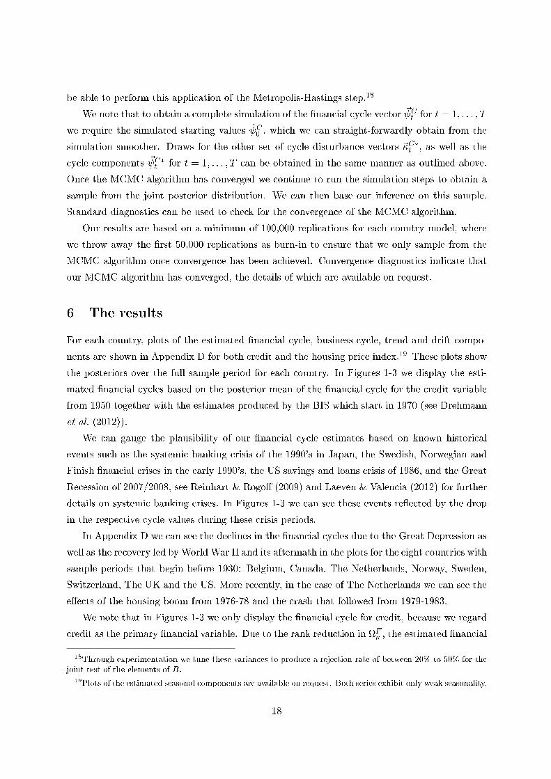
For each country, plots of the estimated �nancial cycle, business cycle, trend and drift compo-

nents are shown in Appendix D for both credit and the housing price index.19 These plots show

the posteriors over the full sample period for each country. In Figures 1-3 we display the esti-

mated �nancial cycles based on the posterior mean of the �nancial cycle for the credit variable

from 1950 together with the estimates produced by the BIS which start in 1970 (see Drehmann

et al. (2012)).

We can gauge the plausibility of our �nancial cycle estimates based on known historical

events such as the systemic banking crisis of the 1990's in Japan, the Swedish, Norwegian and

Finish �nancial crises in the early 1990's, the US savings and loans crisis of 1986, and the Great

Recession of 2007/2008, see Reinhart & Rogo� (2009) and Laeven & Valencia (2012) for further

details on systemic banking crises. In Figures 1-3 we can see these events re ected by the drop

in the respective cycle values during these crisis periods.

In Appendix D we can see the declines in the �nancial cycles due to the Great Depression as

well as the recovery led by World War II and its aftermath in the plots for the eight countries with

sample periods that begin before 1930: Belgium, Canada, The Netherlands, Norway, Sweden,

Switzerland, The UK and the US. More recently, in the case of The Netherlands we can see the

e�ects of the housing boom from 1976-78 and the crash that followed from 1979-1983.

We note that in Figures 1-3 we only display the �nancial cycle for credit, because we regard

credit as the primary �nancial variable. Due to the rank reduction in F� , the estimated �nancial

18Through experimentation we tune these variances to produce a rejection rate of between 20% to 50% for thejoint test of the elements of B.

19Plots of the estimated seasonal components are available on request. Both series exhibit only weak seasonality.

18

cycle based on the housing price index will be asymptotically identical to that of the �nancial

cycle of credit. This is demonstrated in Table 1 where the �rst two columns list the correlation

coe�cients between the �nancial cycle medians we obtain for the credit and housing price index

series. In the �rst column we see the correlation coe�cient over the entire sample period, while

the second column lists the correlations coe�cient from 1980. Both on average, as well as for

all individual countries, the correlation coe�cients are higher in the second column and are

typically nearly equal to 1. Only Finland (0.91), Italy (0.90), South Korea (0.80) and Norway

(0.83) are under the average value of 0.96.

The estimated �nancial cycles based on the credit and housing price index di�er initially due

to the assumed independence between the initial values of these two cycles. It would be possible

to use the �nancial cycle components' rank-reduced disturbance covariance matrix to impose

the implied reduced-rank covariance on the initial value of these cycles in our estimation. In

this manner the two �nancial cycle estimates would be identical with the exception of a scaling

factor. We leave this, however, to future research.

In Table 1 we also list the correlation coe�cients between the estimated �nancial cycles and

that of the BIS. In the third column of the table we show the correlation coe�cient with the

estimated cycle based on the credit series, and in the forth column we show the coe�cient based

on the housing price index. The average correlation between the BIS cycle estimates and ours

based on the credit series is 0.73, which indicates a substantial degree of agreement between the

estimates.20 Of the eighteen countries, only our estimates of the �nancial cycle for Germany

and South Korea show a relatively weak correspondence with those of the BIS. The correlation

between our �nancial cycle estimates and those of the BIS for the other countries is strong.

Furthermore, for most countries both �nancial cycle estimates cross zero at approximately the

same time.

Our estimates of a single �nancial cycle for each country we study rely on the rank reduction

in the covariance matrix of the �nancial cycle components' disturbances. We test the validity

of this rank restriction in two ways. First we calculate the log of the posterior data density

both with and without the rank restriction. We use the same priors for the unrestricted model

as we selected for the restricted model. This should tend to favor the restricted model, given

that some of these priors are selected using empirical Bayesian priors. These values are listed

in Table 2. We denote the rank of F� in the table by r

�F�

�. The column denoted by BF, for

Bayes Factor, shows the di�erence between the two log posterior data densities: the restricted

value minus the unrestricted value. Positive values indicate support for the restricted model,

while negative ones indicate support for the unrestricted model. We are clearly unable to justify

20In future work we intend to also compare our estimates with other estimates obtained in the literature suchas in de Winter et al. (2017), R�unstler & Vlekke (2018) and WGEM (2018).

19

Figure 1: Financial cycle estimates for credit and from the BIS for advanced economies (i)

1950 1960 1970 1980 1990 2000 2010 2020−1,0

−0,5

0,0

0,5

1,0

−4

−2

0

2

4

Australia

1950 1960 1970 1980 1990 2000 2010 2020−15

−10

−5

0

5

10

15

20

−3

−2

−1

0

1

2

3

4

Belgium

1950 1960 1970 1980 1990 2000 2010 2020−4

−2

0

2

4

6

−2

−1

0

1

2

3

Canada

1950 1960 1970 1980 1990 2000 2010 2020−15

−10

−5

0

5

10

15

−3

−2

−1

0

1

2

3

Denmark

1950 1960 1970 1980 1990 2000 2010 2020−15

−10

−5

0

5

10

15

−3

−2

−1

0

1

2

3

Finland

1950 1960 1970 1980 1990 2000 2010 2020−6

−4

−2

0

2

4

6

−3

−2

−1

0

1

2

3

France

The right axis corresponds to our estimated �nancial cycle for credit (dark blue line) and the axis on theleft corresponds to the estimated �nancial cycle of the BIS (light blue line).

20

Figure 2: Financial cycle estimates for credit and from the BIS for advanced economies (ii)

1950 1960 1970 1980 1990 2000 2010 2020−4

−3

−2

−1

0

1

2

3

−4

−3

−2

−1

0

1

2

3

Germany

1950 1960 1970 1980 1990 2000 2010 2020−15

−10

−5

0

5

10

15

−3

−2

−1

0

1

2

3

Ireland

1950 1960 1970 1980 1990 2000 2010 2020−15

−10

−5

0

5

10

15

−3

−2

−1

0

1

2

3

Italy

1950 1960 1970 1980 1990 2000 2010 2020−2

−1

0

1

2

3

−2

−1

0

1

2

3

Japan

1950 1960 1970 1980 1990 2000 2010 2020−2

−1

0

1

2

3

−2

−1

0

1

2

3

Netherlands

1950 1960 1970 1980 1990 2000 2010 2020−15

−10

−5

0

5

10

15

20

25

−3

−2

−1

0

1

2

3

4

5

Norway

The right axis corresponds to our estimated �nancial cycle for credit (dark blue line) and the axis on theleft corresponds to the estimated �nancial cycle of the BIS (light blue line).

21

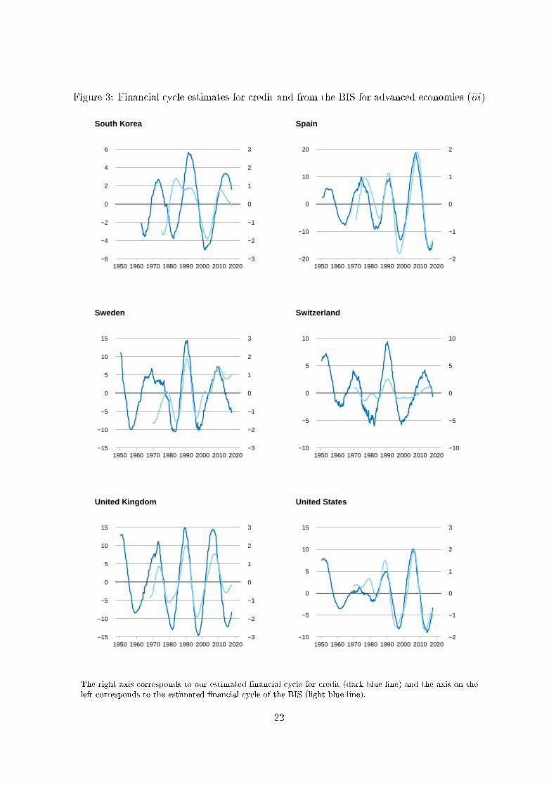
Figure 3: Financial cycle estimates for credit and from the BIS for advanced economies (iii)

1950 1960 1970 1980 1990 2000 2010 2020−6

−4

−2

0

2

4

6

−3

−2

−1

0

1

2

3

South Korea

1950 1960 1970 1980 1990 2000 2010 2020−20

−10

0

10

20

−2

−1

0

1

2

Spain

1950 1960 1970 1980 1990 2000 2010 2020−15

−10

−5

0

5

10

15

−3

−2

−1

0

1

2

3

Sweden

1950 1960 1970 1980 1990 2000 2010 2020−10

−5

0

5

10

−10

−5

0

5

10

Switzerland

1950 1960 1970 1980 1990 2000 2010 2020−15

−10

−5

0

5

10

15

−3

−2

−1

0

1

2

3

United Kingdom

1950 1960 1970 1980 1990 2000 2010 2020−10

−5

0

5

10

15

−2

−1

0

1

2

3

United States

The right axis corresponds to our estimated �nancial cycle for credit (dark blue line) and the axis on theleft corresponds to the estimated �nancial cycle of the BIS (light blue line).

22

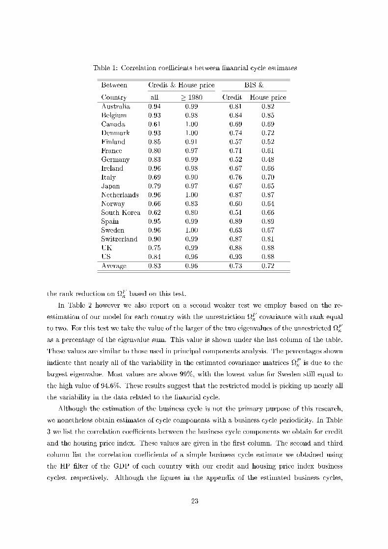
Table 1: Correlation coe�cients between �nancial cycle estimates

Between Credit & House price BIS &

Country all � 1980 Credit House price

Australia 0.94 0.99 0.81 0.82Belgium 0.93 0.98 0.84 0.85Canada 0.61 1.00 0.69 0.69Denmark 0.93 1.00 0.74 0.72Finland 0.85 0.91 0.57 0.52France 0.80 0.97 0.71 0.61Germany 0.83 0.99 0.52 0.48Ireland 0.96 0.98 0.67 0.66Italy 0.69 0.90 0.76 0.70Japan 0.79 0.97 0.67 0.65Netherlands 0.96 1.00 0.87 0.87Norway 0.66 0.83 0.60 0.64South Korea 0.62 0.80 0.51 0.66Spain 0.95 0.99 0.89 0.89Sweden 0.96 1.00 0.63 0.67Switzerland 0.90 0.99 0.87 0.81UK 0.75 0.99 0.88 0.88US 0.84 0.96 0.93 0.88

Average 0.83 0.96 0.73 0.72

the rank reduction on F� based on this test.

In Table 2 however we also report on a second weaker test we employ based on the re-

estimation of our model for each country with the unrestriction F� covariance with rank equal

to two. For this test we take the value of the larger of the two eigenvalues of the unrestricted F�

as a percentage of the eigenvalue sum. This value is shown under the last column of the table.

These values are similar to those used in principal components analysis. The percentages shown

indicate that nearly all of the variability in the estimated covariance matrices F� is due to the

largest eigenvalue. Most values are above 99%, with the lowest value for Sweden still equal to

the high value of 94.6%. These results suggest that the restricted model is picking up nearly all

the variability in the data related to the �nancial cycle.

Although the estimation of the business cycle is not the primary purpose of this research,

we nonetheless obtain estimates of cycle components with a business cycle periodicity. In Table

3 we list the correlation coe�cients between the business cycle components we obtain for credit

and the housing price index. These values are given in the �rst column. The second and third

column list the correlation coe�cients of a simple business cycle estimate we obtained using

the HP �lter of the GDP of each country with our credit and housing price index business

cycles, respectively. Although the �gures in the appendix of the estimated business cycles,

23

Table 2: Tests of Rank Reduction on F�

log posterior data density

Country r�F�

�= 2 r

�F�

�= 1 BF 100�1

�1+�2Australia -660 -696 -36 99.6Belgium -829 -850 -20 98.5Canada -843 -876 -33 99.9Denmark -643 -688 -45 99.9Finland -108 -141 -32 99.1France -285 -334 -49 99.9Germany -254 -285 -32 98.8Ireland -691 -718 -28 99.8Italy -690 -706 -16 98.8Japan -505 -584 -79 99.1Netherlands -1070 -1114 -44 99.9Norway -909 -933 -23 98.3South Korea -538 -557 -20 99.5Spain -641 -665 -23 98.4Sweden -893 -907 -14 94.6Switzerland -748 -775 -27 98.3UK -937 -960 -23 99.0US -623 -654 -31 99.4

The column header \BF" refers to the Bayes factor for the SSMwith r

�F�

�= 1 vs. the SSM with r

�F�

�= 2.

24

which also show the HP �lter business cycle estimated based on GDP, indicate a reasonable

degree of co-movement, overall the degree of correlation is low. This suggests that the cyclical

factors in uencing credit and house prices at this frequency are not primarily determined by the

business cycle in output.

The estimates of the trend and drift components, shown in Appendix D, are gradually

changing and seem to reasonably capture the long-run trends shown in the data, which is also

shown in the �gures. The drift components, representing the underlying growth rates of the

trends, also generally show the slowdown associated with the secular stagnation of the past

decades.

Table 3: Correlation coe�cients between business cycle estimates

Between Credit & House price HP �lter GDP &

Country Credit House price

Australia 0.22 0.06 0.38Belgium 0.20 0.08 0.19Canada 0.34 0.23 0.29Denmark 0.78 0.50 0.55Finland 0.13 0.10 0.53France -0.14 0.15 0.47Germany 0.23 0.39 0.22Ireland 0.38 0.44 0.55Italy 0.12 0.14 0.07Japan 0.19 0.33 0.46Netherlands -0.04 0.32 0.34Norway 0.14 0.23 0.15South Korea 0.36 0.08 0.42Spain -0.22 0.33 0.44Sweden 0.24 0.04 0.31Switzerland 0.29 0.47 0.36UK 0.20 0.34 0.54US 0.13 0.53 0.38

Average 0.20 0.26 0.37

The mean posterior values for the period of the �nancial cycles, �F of the 18 advanced

economies in our sample were between 63 to 78 quarters, or roughly 16 to 20 years. Values for

these posterior means are given in Table E.3 in Appendix E. For the business cycle we obtained

posterior mean values for �B of between 6 to 10 years. These values are also listed in Table

E.3. They are in close agreement with standard values for the business cycle in the literature.

Appendix E also lists the posterior means and standard deviations for the other parameters in

25

the models, see Tables E.1, E.2 and E.3.

7 Conclusion

We propose a bi-variate model based estimation of the �nancial cycle of 18 advanced economies.

We model total credit to the private non-�nancial sector and the housing price index, the two

series that are generally regarded as best re ecting the �nancial cycle. We employ a state space

model based on unobserved components to capture the salient features in the data. In particular

we specify the �nancial cycle as an unobserved trigonometric component, with rank reduction

imposed on the covariance matrix of this cycle component's disturbance vector to help us to

identify a single underlying �nancial cycle. This use of rank reduction to identify a country's

�nancial cycle is new to the literature.

The rank reduction we impose on the covariance of the �nancial cycle components' distur-

bance terms can be justi�ed in a manner that is similar to principal components analysis: the

largest eigenvalue of the covariance is never less than 94% of the sum of both eigenvalues for all

18 economies in our sample. The reduction does not however seem to be supported by Bayesian

model testing based on the Bayes Factor.

In future research we intend to base our estimates of the �nancial cycle on more series, such

as output, industrial production, spreads and the price to earning ratio. We also will explore the

use of the rank-reduced covariance of the �nancial cycle disturbances to obtain the covariance

of the starting vector of the �nancial cycle. This should result in �nancial cycles for both the

credit and house price series which are identical up to a scaling factor, whereas our estimation

results here are only asymptotically identical.

The �nancial cycle estimates have periods lasting roughly 16 to 20 years. Financial events

such as the Japanese banking crisis of 1991, the Scandinavian banking crises of the early 1990's,

the US savings and loans crisis and the Great Recession are all re ected in the �nancial cycle

estimates of the respective countries. Our estimates also largely agree with �nancial cycle

estimates produced by the BIS. We conclude that our method succeeds in generating plausible

estimates for a unique �nancial cycle for each country we analyze.

References

Baxter, M., & King, R. G. 1999. Measuring business cycles: approximate band-pass �lters for

economic time series. Review of Economics and Statistics, 81, 575{593.

Borio, Claudio. 2014. The �nancial cycle and macroeconomics: What have we learnt? Journal

of Banking & Finance, 45(C), 182{198.

26

Claessens, Stijn, Kose, M. Ayhan, & Terrones, Marco E. 2012. How do business and �nancial

cycles interact? Journal of International economics, 87(1), 178{190.

de Winter, Jasper, Koopman, Siem Jan, Hindrayanto, Irma, & Chouhan, Anjali. 2017. Modeling

the business and �nancial cycle in a multivariate structural time series model. DNB Working

Paper, 573(Oct.), 1{40.

Doornik, J. A., & Ooms, M. 2007. Introduction to Ox: An Object-Oriented Matrix Language.

London: Timberlake Consultants Press and Oxford: www.doornik.com.

Drehmann, Mathias, Borio, Claudio, & Tsatsaronis, Kostas. 2012 (June). Characterising the

�nancial cycle: don't lose sight of the medium term! BIS Working Papers 380. Bank for

International Settlements.

Durbin, J., & Koopman, S. J. 2001. Time Series Analysis by State Space Methods. Oxford

Statistical Science Series. Oxford University Press.

Galati, Gabriele, Hindrayanto, Irma, Koopman, Siem Jan, & Vlekke, Marente. 2016. Measuring

�nancial cycles in a model-based analysis: Empirical evidence for the United States and the

euro area. Economics Letters, 45, 83 { 87.

Harvey, A. C., & Streibel, M. 1998. Testing for Deterministic versus Indeterministic Cycles.

Journal of Time Series Analysis, 505{529.

Harvey, Andrew C. 1991. Forecasting, Structural Time Series Models and the Kalman Filter.

Cambridge Books, no. 9780521405737. Cambridge University Press.

Harvey, Andrew C., Trimbur, Thomas M., & van Dijk, Herman K. 2007. Trends and cycles in

economic time series: A Bayesian approach. Journal of Econometrics, 140, 618{649.

Jord�a, �Oscar, Schularick, Moritz, & Taylor, Alan M. 2017. Macro�nancial History and the

New Business Cycle Facts. In: Eichenbaum, Martin, & Parker, Jonathan A. (eds), NBER

Macroeconomics Annual 2016, vol. 31. Uniersity of Chicago Press.

Jord�a, �Oscar, Schularick, Moritz, Taylor, Alan M., & Ward, Felix. 2018 (June). Global Financial

Cycles and Risk Premiums. NBER Working Papers 24677. National Bureau of Economic

Research, Inc.

Knoll, Katharina, Schularick, Moritz, & Steger, Thomas. 2017. No Price Like Home: Global

House Prices, 18702012. American Economic Review, 107(2), 331{53.

Koop, Gary, Poirier, Dale J., & Tobias, Justin L. 2007. Bayesian Econometric Methods. Cam-

bridge University Press.

27

Koopman, S. J., Shephard, N., & Doornik, J. A. 1999. Statistical Algorithms for Models in

State Space Using SsfPack 2.2. Econometrics Journal, 2, 113{166.

Koopman, Siem Jan, & Lucas, Andre. 2005. Business and Default Cycles for Credit Risk.

Journal of Applied Econometrics, 20, 311{323.

Laeven, Luc, & Valencia, Fabian. 2012. Systemic Banking Crises Database: An Update. IMF

Working Paper, 163, 1{32.

Luginbuhl, Rob, & Vos, Aart de. 2003. Seasonality and Markov switching in an unobserved

component time series model. Empirical Economics, 28(2), 365{386.

Reinhart, Caarmen M., & Rogo�, Kenneth S. 2009. This Time is Di�erent: Eight Centuries of

Fanancial Folly. Princeton: Princeton University Press.

Rozite, Kristiana, Bezemer, Dirk J., & Jacobs, Jan P.A.M. 2016. Towards a �nancial cycle for

the US, 1973-2014. Research Report 16013-GEM. University of Groningen, Research Institute

SOM (Systems, Organisations and Management).

R�unstler, Gerhard, & Vlekke, Marente. 2018. Business, housing, and credit cycles. Journal of

Applied Econometrics, 33(2), 212{226.

Sch�uler, Yves Stephan, Hiebert, Paul P., & Peltonen, Tuomas A. 2015. Characterising the

�nancial cycle: A multivariate and time-varying approach. Annual Conference 2015 (Muen-

ster): Economic Development - Theory and Policy 112985. Verein fr Socialpolitik / German

Economic Association.

Soederhuizen, Beau, Teulings, Rutger, & Luginbuhl, Rob. 2019. Estimating the Impact of the

Financial Cycle on Fiscal Policy. CPB Discussion Paper. CPB Netherlands Bureau for Eco-

nomic Policy Analysis.

WGEM, Team on Real & Financial Cycles. 2018. Real and �nancial cycles in EU countries:

Stylised facts and modelling implications. ECB Occassional paper series, 1{68.

A Alternative Speci�cation of the Financial Cycle

An alternative speci�cation for a model with a shared �nancial cycle can be formulated using

the notation ~yt = (y1; y2). First, however, note that using this notation, we can re-write (1) as

follows.

~yt = ~�t + ~ Ft + ~ B

t +

[s=2]Xj=1

~ j;t + ~"t (A.1)

28

The alternative formulation of the second general state space model can then be expressed as

follows.

~yt = ~�t +A ~ Ft +B ~ B

t +

[s=2]Xj=1

~ j;t + ~"t; (A.2)

where the matrices A and B are both lower triangular matrices with unity along the main

diagonal. The matrix A then is a loading-matrix that determines how much each of the two

cycles Fi;t contributes to the data series yi;t. The same is true for the loading-matrix B, which

determines the weighted contribution of the two cycles Bi;t to the data series yi;t. In order to

ensure that this model is identi�ed, we must also restriction the covariance matrices � to be a

diagonal matrices. In other words, the underlying cycle components must be independent.

This second model speci�cation is, with the exception of the alternate speci�cation of the

measurement equation shown in (A.2), based on the same equations for the unobserved com-

ponents shown above in (3) - (5).21 This model is similar to the models proposed in Koopman

& Lucas (2005) and de Winter et al. (2017). The di�erence between our model and theirs is

due to how the cycle components are formulated. In the �rst model the measurement equation

(A.1) includes cycle components that are derived by correlated disturbance terms. This has the

e�ect that the cyclical components can di�er in their amplitude and phase even when the cycle

component disturbances are perfectly correlated. The second model in (A.2) by comparison will

be based on underlying cycle components which can only di�er in their amplitude when each

series selects the same underlying cycle component in the measurement equation (A.2).

We would like to identify a single �nancial cycle. There are two modeling options we can

follow to achieve this. One option is based on (1) and requires the imposition of the restriction

that the rank of the covariance matrix of the �nancial cycle component f� be reduced from

two to one. In this manner both �nancial cycles for the series in the model are assumed to be

derived from the same underlying stochastic process.

The second alternative is based on (A.2) with the restriction that the Amatrix select the same

underlying �nancial cycle for both series in the model. Although we have experimented with

this second modeling technique to estimate a �nancial cycle, we found it to be too restrictive.

Instead we base our estimates in this article on the model in which we impose rank reduction on

f�. Our impression is that the extra exibility of this method produces more plausible results,

because the model still allows for di�ering phase shifts in the �nancial cycle of each series. On

the other hand, the disadvantage of our approach is that it still requires us to chose which of

the two estimated �nancial cycles represents the underlying �nancial cycle, because initially at

least, they may not be the same.

21In our formulation of the measurement equation we have also included seasonal components in the model toaccommodate seasonally unadjusted data.

29

We note, however, that these two modeling approaches can be made observationally equiva-

lent. This can be achieved by specifying in our model a joint normal prior on the initial values

of the �nancial cycle components with the prior covariance given by

F�

1� �F 2 ; (A.3)

where F� is the reduced rank covariance matrix.22

B Prior Parameters

The inverse Wishart prior parameters SB� and SF

� for the covariance matrices B� and F

� ,

respectively, are listed in Table B.1. Note that �B = �F = 13 with the exception of Korea,

where �F = 6. The parameters sB�1 and sF�1 pertain to the credit series, sB�2 and sF�2 to the

housing price index, and sF�12 is the scale factor for the covariance between the �nancial cycle

disturbances for credit and the housing price index.23 The comparable prior scale factor for the

covariance of the business cycle disturbance is set to zero for all countries. We have therefore

that

SB� =

"sB�1 0

0 sB�2

#SF� =

"sF�1 sF�12

sF�12 sF�2

#(B.1)

22In the case of the alternative formulation, the �nancial cycle components are independent, and therefore soare their initial values.

23The latter value is set to exactly ensure that the rank of SF = 1.

30

Table B.1: Cycle Disturbance Covariance Priors

SB� SF

�

Country sB�1 sB�2 sF�1 sF�2 sF�12

Australia 15.0 15.0 0.2 12.0 1.549

Belgium 50.0 15.0 6.0 6.0 6.000

Canada 25.0 1.0 1.0 60.0 7.746

Denmark 2.0 60.0 15.0 0.1 1.225

Finland 25.0 45.0 2.0 3.0 2.450

France 8.0 4.0 0.1 3.0 0.548

Germany 4.0 3.0 1.5 3.0 2.121

Ireland 120.0 40.0 2.0 30.0 7.746

Italy 25.0 20.0 2.0 2.0 2.000

Japan 10.0 14.0 0.2 2.0 0.632

Netherlands 20.0 20.0 0.2 6.0 1.095

Norway 20.0 60.0 8.0 4.0 5.657

South Korea 50.0 15.0 0.3 1.8 0.735

Spain 22.0 30.0 5.0 20.0 10.000

Sweden 20.0 50.0 12.0 7.5 9.487

Switzerland 12.0 22.0 1.5 2.5 1.937

UK 50.0 50.0 5.0 15.0 8.660

US 9.0 9.0 1.2 10.0 3.464

31

Table B.2: Trend & Drift disturbance Covariance Priors & Sample Starting Date

S� S� begin

Country s�1 s�2 s�1 s�2 sample period

Australia 0.300 0.300 0.512 0.512 1950 Q4

Belgium 0.400 0.300 0.512 0.512 1921 Q4

Canada 0.300 0.300 0.512 0.200 1914 Q4

Denmark 1.500 1.500 0.512 0.512 1950 Q4

Finland 0.600 0.300 0.008 3.2E-04 1955 Q4

France 0.600 0.300 0.512 0.512 1955 Q4

Germany 1.500 1.500 0.512 0.512 1955 Q4

Ireland 0.400 0.300 0.512 0.512 1970 Q4

Italy 0.600 0.300 0.392 0.512 1953 Q4

Japan 0.100 0.090 0.512 0.512 1949 Q4

Netherlands 0.100 0.100 0.800 0.512 1900 Q4

Norway 0.100 0.095 0.512 0.512 1925 Q4

South Korea 0.100 0.100 0.512 0.128 1962 Q4

Spain 0.500 0.200 0.512 0.512 1950 Q4

Sweden 0.180 0.150 0.512 0.800 1921 Q4

Switzerland 0.100 0.130 0.512 0.512 1921 Q4

UK 0.070 0.100 0.512 0.512 1921 Q4

US 0.016 0.060 0.512 0.200 1914 Q4

32

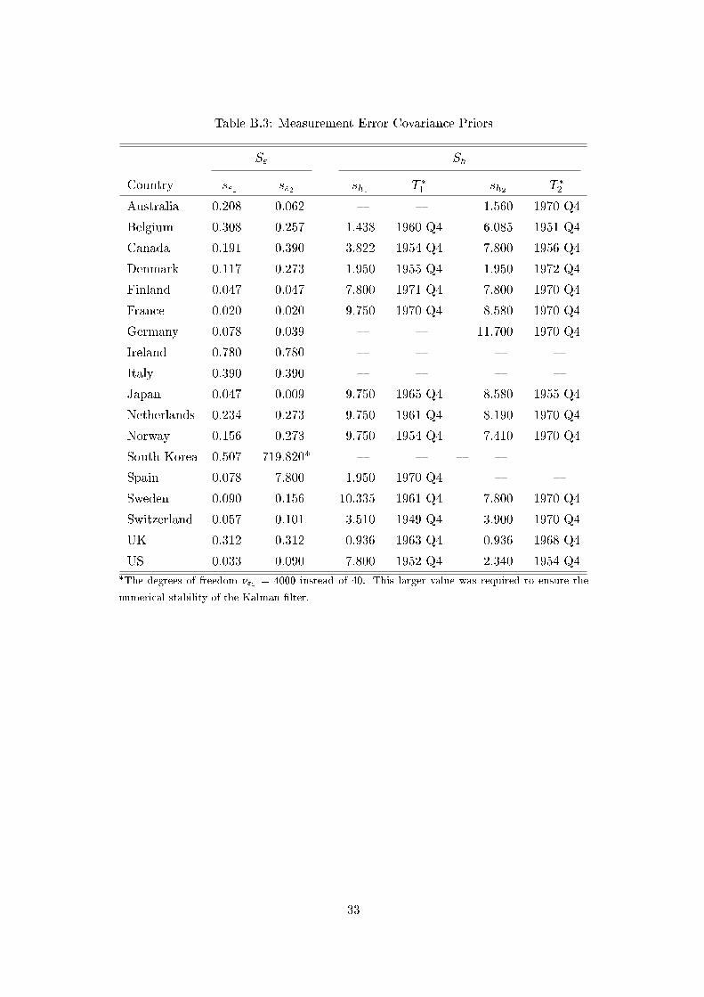
Table B.3: Measurement Error Covariance Priors

S" Sh

Country s"1 s"2 sh1 T �

1 sh2 T �

2

Australia 0:208 0:062 { { 1:560 1970 Q4

Belgium 0:308 0:257 1:438 1960 Q4 6:085 1951 Q4

Canada 0:191 0:390 3:822 1954 Q4 7:800 1956 Q4

Denmark 0:117 0:273 1:950 1955 Q4 1:950 1972 Q4

Finland 0:047 0:047 7:800 1971 Q4 7:800 1970 Q4

France 0:020 0:020 9:750 1970 Q4 8:580 1970 Q4

Germany 0:078 0:039 { { 11:700 1970 Q4

Ireland 0:780 0:780 { { { {

Italy 0:390 0:390 { { { {

Japan 0:047 0:009 9:750 1965 Q4 8:580 1955 Q4

Netherlands 0:234 0:273 9:750 1961 Q4 8:190 1970 Q4

Norway 0:156 0:273 9:750 1954 Q4 7:410 1970 Q4

South Korea 0:507 719:820* { { { {

Spain 0:078 7:800 1:950 1970 Q4 { {

Sweden 0:090 0:156 10:335 1961 Q4 7:800 1970 Q4

Switzerland 0:057 0:101 3:510 1949 Q4 3:900 1970 Q4

UK 0:312 0:312 0:936 1963 Q4 0:936 1968 Q4

US 0:033 0:090 7:800 1952 Q4 2:340 1954 Q4

*The degrees of freedom �"2 = 4000 instead of 40. This larger value was required to ensure the

numerical stability of the Kalman �lter.

33

C Data series

Table C.1: CPI data for de ating

Sources and starting dates

Country Start monthly OECD Other source Freqcuency start

Australia 1950m7 Australian Bureau of Statistics Quarterly 1948q3

Belgium 1955m1 STATBEL Monthly 1920m1

Canada 1950m7 Statistics Canada Yearly 1914

Denmark 1955m1 FRED St. Louis Fed Yearly 1950

Finland 1955m1 - - -

France 1955m1 - - -

Germany 1955m1 Bundesbank Yearly 1949

Ireland 1955m1 Central Statistics O�ce Ireland Monthly 1922m1

Italy 1955m1 FRED St. Louis Fed Yearly 1953

Japan 1955m1 Statistics of Japan (E-Stat) Monthly 1946m8

Netherlands 1959m1 CBS - Statistics Netherlands Yearly 1900

Norway 1955m1 Statistics Norway Monthly 1925m1

South Korea 1951m8 - - -

Spain 1954m3 FRED St. Louis Fed Yearly 1950

Sweden 1955m1 SCB, Statistics Sweden Quarterly 1917q3

Switzerland 1955m1 Bundesambt fur statistik Monthly 1921m1

United Kingdom 1955m1 FRED St. Louis Fed Quarterly 1914q1

United States 1955m1 FRED St. Louis Fed Monthly 1913m1

The series from the other sources are scaled to the monthly OECD series to have one full CPI series.

D Estimated Unobserved Components

The Figures D.1 - D.18 in this appendix show plots of the medians24 of the posterior distributions

of the unobserved components in the model: the �nancial cycles, the business cycles, the trends

and the drifts. The four plots on the left-hand side of each �gure are the estimates of the

unobserved components for credit. Those on the right-hand side are based on the housing price

index. The plots also show the Bayesian credible interval of 68%, or in other words � one

standard deviation of the posteriors. For comparision, the plots of the �nancial cycle estimates

also include the BIS estimates of the �nancial cycle. The same is true of the business cycle,

24Given the assumed normality of the disturbances, the median and mean of the posteriors will be equal.

34

where we also plot the HP-�lter cycle of GDP for comparison. The plots of the estimated trends

also show the logarithm of original data, while the drift, or growth rate plots show the �rst

di�erence of the logarithm of the original data.

By comparing the �nancial cycle estimates in each �gure based on credit with those based on

the housing price index, we can see that in some cases one series clearly dominates in determining

the cycle. See for example the case of The Netherlands in Figure D.11 where the credible interval

on the �nancial cycle for credit is more di�use, while the cycle based on the housing price index

is nonetheless strongly de�ned. It is important to remember that the �nancial cycle estimates

are jointly determined by the credit and the housing price series due to the rank reduction on

the covariance matrix F� . Therefore these cycle estimates re ect the information in both series.

These estimates suggest that the housing price index is the dominate factor in determining the

�nancial cycle for The Netherlands.

35

Figure D.1: Underlying model estimates for Australia

1940 1960 1980 2000 2020−1,5

−1,0

−0,5

0,0

0,5

1,0

1,5

2,0

−3

−2

−1

0

1

2

3

4

Financial Cycle − Credit

median (left) BIS (right)

1940 1960 1980 2000 2020−15

−10

−5

0

5

10

15

−3

−2

−1

0

1

2

3

Financial Cycle − House Prices

median (left) BIS (right)

1940 1960 1980 2000 2020−20

−15

−10

−5

0

5

10

15

−8

−6

−4

−2

0

2

4

6

Business Cycles − Credit

median (left) HP cycle GDP (right)

1940 1960 1980 2000 2020−15

−10

−5

0

5

10

15

−6

−4

−2

0

2

4

6

Business Cycles − House Prices

median (left) HP cycle GDP (right)

1940 1960 1980 2000 2020−300

−200

−100

0

100

200

Trend − Credit

●●●

●●●●●

●●●●

●●●●

●

●●●●

●●●●●●

●●●●

●●●●●

●●●●●

●●●●

●●●●

●●●●

●●●

●●●

●●●

●●●●●

●●●●●

●●●●

●●●●

●●●●

●●●●

●●●●●●●●●●●●●●●●●●

●●●●●●

●●●●●●●●●●

●●●●●●●●●●●●●●●●●●●●●●●●●●●●●●

●●●●●●●

●●●●●●●

●●●●●●●●

●●●●●●●●●

●●●●●

●●●●●●●

●●●●●●●●●●●●●●●●●

●●●●●●●●●●

●●●●●●

●●●●●●●●●●●●●●●●●●●●●●●●●●●●●●●●●●●●●●●●●

●median Log data

1940 1960 1980 2000 2020−100

−50

0

50

100

150

Trend − House Prices

●

●

●● ● ●

●

● ● ●

●

●

●

● ● ● ● ●

●

●●●●●

●●●●●

●●

●●●

●●●●

●●●●

●●●●●

●●●●●●●●●●●●●●

●●●●●

●●●●

●●●

●●●●●●●

●●●●●●

●●●●●●●●

●

●

●●●●●●●

●●●●●●●●●●●●

●●●●●●

●●●●●●●●●●●

●●●●●●●

●●●●●●

●

●●●

●●●●

●

●●●●●●●●●●●

●●●●

●●●●

●●●●

●●

●●●●●

●●●●●●●

●●●●

●●●●

●●●●●●

●●●●●●●

●median Log data

1940 1960 1980 2000 2020−6

−4

−2

0

2

4

6

8

10

Drift − Credit

●

●

●

●

●

●

●

●

●

●

●

●

●

●

●

●

●

●

●

●

●

●

●

●

●

●

●

●

●

●

●

●

●

●

●●

●

●

●

●

●

●

●

●

●●

●

●

●

●

●

●

●

●

●

●

●

●

●

●

●

●

●

●

●●

●

●

●

●

●

●

●

●

●

●

●

●

●

●

●

●

●

●

●

●

●

●

●

●

●

●

●

●

●

●

●

●

●

●

●

●●●

●

●

●

●

●

●●

●

●

●

●

●

●

●

●

●

●

●

●

●●

●

●

●

●

●●

●

●

●

●

●

●

●

●

●

●

●

●

●

●

●

●

●

●

●

●

●

●

●●

●

●

●

●

●●

●

●

●

●

●

●●

●

●

●

●

●

●

●

●

●

●

●

●

●

●

●

●

●

●

●

●

●

●

●

●

●

●

●

●

●

●

●

●

●

●

●●

●

●●

●

●

●

●

●

●

●

●

●

●

●

●

●

●●●

●●

●

●

●

●

●

●

●

●●

●●

●

●

●

●

●

●●

●

●

●

●

●●●

●

●

●

●

●

●

●

●

●●

●●

●●

●

●

●●

●median Mutations Log Data

1940 1960 1980 2000 2020−6

−4

−2

0

2

4

6

8

Drift − House Prices

●

●

●

●

●

●

●

●

●

●

●

● ●

● ●●

●

● ●●

●

●

●

●

●

●

●

●

●●

●

●

●

●

●

●

●

●

●

●

●

●

●

●

●

●

●

●

●

●

●

●

●

●●

●●

●

●

●

●

●

●

●

●

●

●

●

●

●

●

●

●

●

●

●

●

●

●

●

●

●

●

●

●

●

●

●

●

●

●

●

●

●●

●

●

●

●●

●

●

●

●

●

●

●

●

●

●

●

●●

●

●●●

●

●

●

●

●●

●

●

●●

●

●

●

●

●

●

●

●

●●

●

●

●

●

●

●

●

●

●

●●

●

●

●

●

●●

●

●●

●

●

●

●

●

●

●

●

●

●

●

●

●●

●

●

●

●

●

●

●

●

●

●

●

●

●

●

●

●

●

●

●

●

●

●

●

●

●

●

●

●

●

●

●

●

●

●

●

●

●●

●

●

●median Mutations Log Data

All con�dence bands are one standard deviation.

36

Figure D.2: Underlying model estimates for Belgium

1900 1920 1940 1960 1980 2000 2020−40

−20

0

20

40

−4

−2

0

2

4

Financial Cycle − Credit

median (left) BIS (right)

1900 1920 1940 1960 1980 2000 2020−20

−15

−10

−5

0

5

10

15

20

−4

−3

−2

−1

0

1

2

3

4

Financial Cycle − House Prices

median (left) BIS (right)

1900 1920 1940 1960 1980 2000 2020−20

−15

−10

−5

0

5

10

15

20

−4

−3

−2

−1

0

1

2

3

4

Business Cycles − Credit

median (left) HP cycle GDP (right)

1900 1920 1940 1960 1980 2000 2020−20

−10

0

10

20

30

−4

−2

0

2

4

6

Business Cycles − House Prices

median (left) HP cycle GDP (right)

1900 1920 1940 1960 1980 2000 2020−300

−200

−100

0

100

200

300

Trend − Credit

●

●

●●

●

●

●●

●

● ●

● ●

●

●●

●●

●

● ●

● ●●

● ●●

●●

●

●

●●

●●

●

●● ●

●●●●●●●●

●●●●●●●●●●●●

●●●●●●

●●●●●●●

●●●●

●●●●●●●●●●●●●●●●●●●●●●●●●●●

●●●●●●●●●●●●●●●●

●●●●●●●●

●●●●●●●●●

●●●●●●●●●●●●●

●●●●●●●●●●●●●●

●●●●●●●●●●

●●●●●●●●●●●

●●●●●

●●●●●

●●●●●●●●●●●●●●

●●●●●●●●●●

●●●●●●●●●●

●median Log data

1900 1920 1940 1960 1980 2000 2020−100

−50

0

50

100

Trend − House Prices

●

●● ●

●

● ●

●

●●

●

●

●

● ●

●

● ●

●

●●

●

●

●

●

●

● ●●

● ● ●

●●

●

●

●

●

●

●

●●●●●

●●●●●●●●●●●●●●

●●

●

●●●●

●●●●●●●

●●●●●●●●●●●●

●●●●

●

●

●●●

●●●●●●●●

●●●●●●

●●●●●●●●●●

●●●●●●●

●●●

●●●●●●●

●●●●●

●●●●●●●●●●

●●●●●●

●●●●●●●●●

●●●●●●

●●●●●●●●●●●●●●●●●●●●●●●●●●

●●●●●●●

●●●●●●●●●●●●●●

●●●●●●●●●●●●●●

●●

●median Log data

1900 1920 1940 1960 1980 2000 2020−15

−10

−5

0

5

10

Drift − Credit

●

●

●

●

●

●

●

●

●

●

●

●

●

●

●●

●

●

●

●

●

●

●

●

●

●● ●

●

●

●●

●

●●

●

●

●

●

●

●

●

●

●

●

●

●

●●

●

●

●●

●

●

●

●

●

●●

●

●

●

●

●

●

●

●

●

●

●

●

●

●

●

●

●

●

●

●

●

●

●

●

●

●

●

●●

●

●

●

●

●

●

●

●

●

●

●

●

●

●

●

●

●

●

●

●●

●

●

●

●

●

●

●

●●●

●

●

●

●

●

●

●

●

●

●

●

●

●●

●●

●

●

●

●

●●

●●

●●

●

●

●

●

●

●

●

●●●●

●

●●●

●

●

●

●

●

●

●

●

●

●●

●

●

●

●

●

●●●

●

●

●●●

●

●●

●

●

●

●●

●

●

●

●

●

●

●

●●

●

●

●

●

●

●

●

●●

●

●

●

●

●

●

●

●

●

●

●

●

●

●

●

●median Mutations Log Data

1900 1920 1940 1960 1980 2000 2020−8

−6

−4

−2

0

2

4

6

8

Drift − House Prices

●

●

●

●

●

●

●

●

●

●

●

●

●

●

●

●

●

●

●

●

●

●

●

●●

●

●●

●●

●

●

● ●

●

● ●

●

●

●

●

●

●

●

●

●

●

●

●

●

●

●

●●

●

●●

●

●

●

●

●

●

●

●

●

●

●

●

●

●

●

●

●

●

●

●

●

●

●

●

●

●

●

●

●

●

●

●

●

●

●

●

●

●●

●

●

●

●

●

●

●

●

●

●

●

●

●

●

●

●

●

●

●

●

●

●

●

●

●

●

●●

●

●

●

●●

●

●

●●

●

●

●

●

●

●

●

●●

●

●

●

●●

●

●

●

●

●

●

●

●

●

●●

●

●

●

●

●

●

●

●

●

●

●

●●

●

●

●

●●●

●

●

●

●

●

●

●

●

●

●

●

●●●

●

●

●

●

●

●●

●

●

●

●

●

●

●

●

●

●●

●●

●

●●

●

●

●

●

●

●

●

●

●

●

●

●

●

●

●●

●

●

●median Mutations Log Data

All con�dence bands are one standard deviation.

37

Figure D.3: Underlying model estimates for Canada

1900 1920 1940 1960 1980 2000 2020−10

−5

0

5

10

−2

−1

0

1

2

Financial Cycle − Credit

median (left) BIS (right)

1900 1920 1940 1960 1980 2000 2020−30

−20

−10

0

10

20

30

−3

−2

−1

0

1

2

3

Financial Cycle − House Prices

median (left) BIS (right)

1900 1920 1940 1960 1980 2000 2020−15

−10

−5

0

5

10

15

20

−6

−4

−2

0

2

4

6

8

Business Cycles − Credit

median (left) HP cycle GDP (right)

1900 1920 1940 1960 1980 2000 2020−3

−2

−1

0

1

2

3

−6

−4

−2

0

2

4

6

Business Cycles − House Prices

median (left) HP cycle GDP (right)

1900 1920 1940 1960 1980 2000 2020−100

0

100

200

300

400

Trend − Credit

● ●●

●● ●

●● ●

●● ●

●

●

●●

●● ● ●

●●

● ●●

●●

●●

● ●

●●

●●

●

● ●

●

●●●●●●●●

●●●●●●●●●●●●

●●●●●●●●

●●●●●●●●●●●●

●●●●●●●●●●●●

●●●●●●●●●●●●●●●

●●●●●●●●●●●●●●●●●●

●●●●●●●●●●●●

●●●●●●●●●●●●

●●●●●●●●●●●●●●●●

●●●●●●

●●●●●●●●●●●●

●●●●●●●●●●●

●●●●●●●●

●●●●●●●●●●●●●

●●●●●●

●●●●●●●●

●●●●●●●●●●●●

●●●●●●●●●●

●●●●●●●●●

●●●●●●●●●●●●

●●●●●●

●●●●●●

●●●●●●●

●●●●●●

●median Log data

1900 1920 1940 1960 1980 2000 2020−150

−100

−50

0

50

100

150

Trend − House Prices

● ●● ●

● ● ●●

●●

● ● ● ●● ●

●● ●

●●

●

●● ●

●● ●

●

●●

● ● ● ● ● ●●

●

●●

●●●●●

●●●●●●●●

●●●●

●

●●●●●●●

●●●●

●●●●●●●●

●●●●●●●

●●●●●●

●

●●●

●●●●●●

●●●●●●●●●

●

●●●●

●●●

●

●

●●●●

●●●●●

●●●●●●

●●●●

●●●●●●●●●●●●●

●●●●●●●●●●●●●●●●

●●●●●●●●●●●●●●●●●●●●●●●●

●●●●●●●

●●●●●●●●●

●●●●●●●●

●●●●●●●●●

●●●●●●●

●●●

●median Log data

1900 1920 1940 1960 1980 2000 2020−8

−4

0

4

8

12

Drift − Credit

●

●

●

●

●

●

●

●

●

●

●

●

●

●

●

●

●

●

●

● ●

●

●

●

●

● ●●

●

●

●

●

●

●

●

●

●

●

●

●

●

●

●

●

●

●

●

●

●

●

●

●

●

●

●

●

●●

●●

●

●

●

●

●

●

●

●

●●

●

●

●

●

●

●

●

●

●

●

●

●

●

●

●

●

●

●

●

●

●

●

●

●

●

●

●

●

●

●

●

●●

●

●

●

●

●

●●

●

●

●

●

●

●

●

●

●

●

●●

●

●

●●

●

●●●●

●

●

●

●●●

●

●●

●●

●●

●

●

●

●

●●

●

●

●

●

●

●●

●●

●●●●

●

●

●

●●

●

●

●●

●

●

●●●

●

●

●

●

●●

●

●

●●

●

●

●

●

●

●

●●●

●

●●

●

●

●

●●

●

●

●

●

●●

●

●

●●

●

●

●

●

●

●●

●●

●

●

●

●

●

●

●

●

●

●

●●

●

●

●

●

●

●

●●

●

●

●

●●

●

●●●

●

●

●

●

●

●

●

●●

●

●

●

●

●●

●

●●

●●

●

●

●

●

●●

●

●

●

●●●

●

●

●

●

●

●

●

●

●

●

●

●median Mutations Log Data

1900 1920 1940 1960 1980 2000 2020−15

−10

−5

0

5

10

Drift − House Prices

●

●

●

●●

●●

●

●

●

●●

●

●

●

●

●

●●

● ●●

●

●

●

●●

●

●●

●

●● ● ●

● ●

●●

●

●

●

●

●

●

●●

●

●

●

●

●

●

●

●

●

●●

●

●

●

●

●●

●

●

●

●

●

●●

●

●

●

●

●

●

●

●

●

●

●

●

●

●

●

●

●

●

●●

●

●

●

●

●

●

●

●

●

●●●

●

●

●●

●

●

●

●

●

●

●

●

●

●

●

●

●

●

●

●

●●

●

●

●

●

●

●●

●

●

●

●

●

●

●

●

●

●

●

●

●

●

●

●

●

●

●

●

●

●

●

●

●

●

●

●

●

●

●

●

●

●

●

●

●●●

●

●

●

●

●

●

●

●

●

●

●●

●

●

●

●

●

●●

●

●

●●

●

●

●

●

●

●

●●

●

●

●

●

●

●●●

●

●●

●

●

●

●

●

●

●

●

●

●●●●

●

●

●

●

●

●

●

●median Mutations Log Data

All con�dence bands are one standard deviation.

38

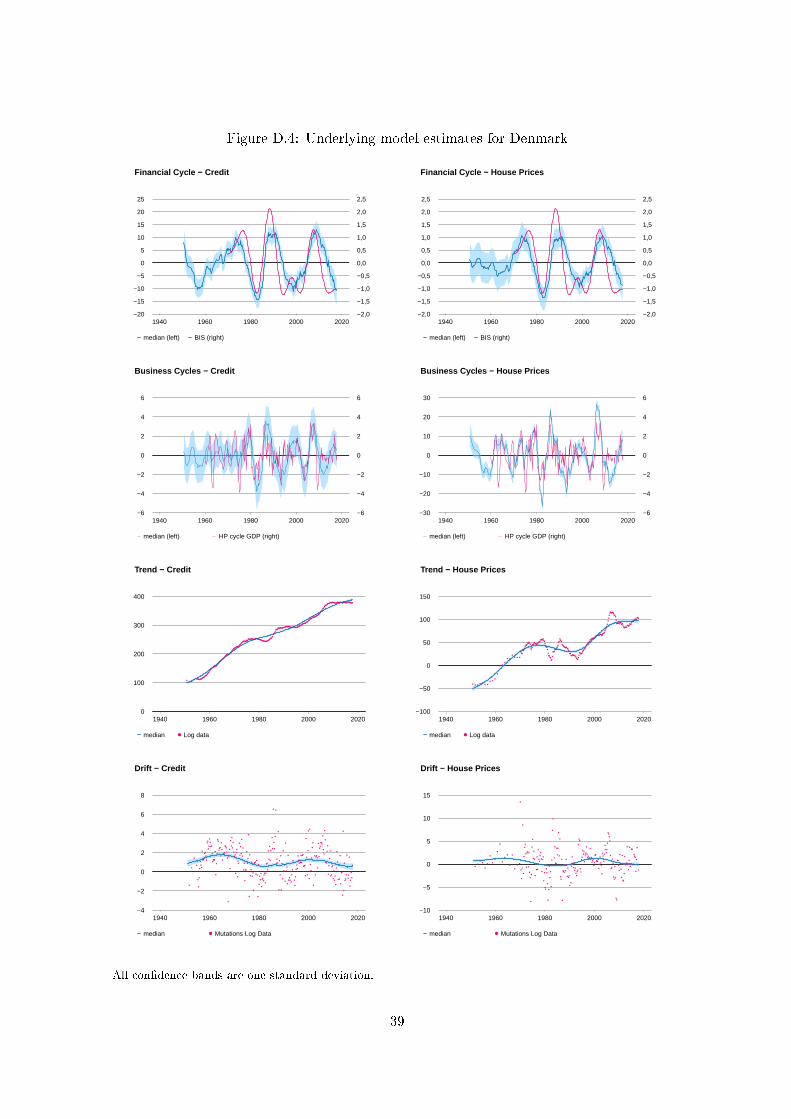
Figure D.4: Underlying model estimates for Denmark

1940 1960 1980 2000 2020−20

−15

−10

−5

0

5

10

15

20

25

−2,0

−1,5

−1,0

−0,5

0,0

0,5

1,0

1,5

2,0

2,5

Financial Cycle − Credit

median (left) BIS (right)

1940 1960 1980 2000 2020−2,0

−1,5

−1,0

−0,5

0,0

0,5

1,0

1,5

2,0

2,5

−2,0

−1,5

−1,0

−0,5

0,0

0,5

1,0

1,5

2,0

2,5

Financial Cycle − House Prices

median (left) BIS (right)

1940 1960 1980 2000 2020−6

−4

−2

0

2

4

6

−6

−4

−2

0

2

4

6

Business Cycles − Credit

median (left) HP cycle GDP (right)

1940 1960 1980 2000 2020−30

−20

−10

0

10

20

30

−6

−4

−2

0

2

4

6

Business Cycles − House Prices

median (left) HP cycle GDP (right)

1940 1960 1980 2000 20200

100

200

300

400

Trend − Credit

●● ●

● ●●●●●●●●●●●●

●●●●

●●●●

●●●●

●●●●●

●●●●●●●●

●●●●●

●●●●

●●●●

●●●

●●●●

●●●●

●●●●●●

●●●●

●●●●

●●●●●●●●●

●●●●●●●●●●●●●●●●●●●●●●●●●●●●●●●●

●●●●

●●●●

●●●

●●●●

●●●●●●●●●

●●●●●●●●●●●●●●●●●●●●●●●●

●●●●●●

●●●●●●●

●●●●●●

●●●●●●●●●●

●●●●

●●●●

●●●●●

●●●●●

●●●●●

●●●●●●●●●●●●●●●●●●●●●

●●●●●●●●●●●●●●●●

●median Log data

1940 1960 1980 2000 2020−100

−50

0

50

100

150

Trend − House Prices

●● ●

● ●● ●

● ●●

●

●●

●

● ●

●● ● ●

●●●●

●●●

●

●●●

●●●

●●●

●●●

●●●●●●●●●

●●●●●●●●

●●●

●

●●●

●

●

●●●●

●●

●

●●●●●●

●●●

●●

●●●●

●●●●●●●●

●●●●

●●●●●

●●●●●●●●●

●

●

●●●●

●●●●●

●●●●●

●●●●●

●●●●●●

●●●●

●●●●●●●

●●●●

●●●●●

●

●

●

●

●●●●●●●

●●●

●

●●●●●●●●

●●●●●●●●●

●●●●●●●

●●●●

●●●●●

●●●

●median Log data

1940 1960 1980 2000 2020−4

−2

0

2

4

6

8

Drift − Credit

●

●

●

●

●

●

●

●

●

●

●

●

●

●●●

●●

●

●

●●

●

●

●

●

●●

●

●

●●●

●

●

●

●

●●

●●●

●

●

●

●

●●●

●●●

●

●

●

●

●

●

●

●

●

●

●

●

●●

●

●

●

●

●

●

●

●

●

●

●

●

●

●

●

●

●●

●

●

●

●

●

●

●

●

●

●

●

●

●●●

●

●

●

●

●

●

●

●

●

●

●●

●

●●

●

●

●●

●

●

●

●

●

●

●

●

●

●

●

●

●

●

●

●

●

●

●

●

●

●

●

●

●

●

●

●

●

●

●

●

●

●

●

●

●

●

●

●

●

●

●

●

●

●

●

●

●

●

●

●

●

●

●

●

●●

●●●

●

●

●

●

●

●

●

●

●

●

●

●

●

●

●

●

●

●●

●

●

●

●

●●

●●●

●

●

●

●

●

●●

●

●

●

●

●

●

●●

●●

●

●

●

●

●

●

●

●

●

●

●

●

●

●●

●

●

●

●

●●

●

●

●

●

●

●

●

●

●

●

●

●median Mutations Log Data

1940 1960 1980 2000 2020−10

−5

0

5

10

15

Drift − House Prices

●

●

●●

●

●

●

●

●

●

●

●

●

●

●

●

●

●●

●

●

●

●

●

●

●

●

●

●

●

●●

●

●

●

●

●

●

●

●

●

●

●

●

●

●

●

●

●

●

●

●

●

●

●

●

●

●

●

●●

●

●

●

●

●

●

●

●

●

●

●

●

●

●

●

●●

●

●

●

●

●

●

●

●

●

●

●●●

●

●

●

●

●

●

●●

●

●

●

●

●

●

●

●

●

●

●

●

●●

●

●●

●

●

●

●

●

●

●

●

●●

●

●

●●

●●

●

●

●

●●●

●

●

●●

●●●

●

●

●

●

●

●

●

●

●

●

●

●

●

●

●

●

●●

●

●

●

●●

●

●

●

●

●

●

●●

●●

●

●

●

●

●

●

●

●●

●

●

●●●

●

●

●

●

●

●●

●●

●●

●●●

●

●

●

●

●

●median Mutations Log Data

All con�dence bands are one standard deviation.

39

Figure D.5: Underlying model estimates for Finland

1940 1960 1980 2000 2020−15

−10

−5

0

5

10

15

−3

−2

−1

0

1

2

3

Financial Cycle − Credit

median (left) BIS (right)

1940 1960 1980 2000 2020−30

−20

−10

0

10

20

−3

−2

−1

0

1

2

Financial Cycle − House Prices

median (left) BIS (right)

1940 1960 1980 2000 2020−30

−20

−10

0

10

20

−15

−10

−5

0

5

10

Business Cycles − Credit

median (left) HP cycle GDP (right)

1940 1960 1980 2000 2020−40

−30

−20

−10

0

10

20

30

40

−8

−6

−4

−2

0

2

4

6

8

Business Cycles − House Prices

median (left) HP cycle GDP (right)

1940 1960 1980 2000 2020−200

−150

−100

−50

0

50

100

150

Trend − Credit

●

●

●

●

●

●

●●

● ●●

● ●●

●

●●●●●

●●●●●●●

●●●●●●●●●●●●

●●●●●●●●

●●●●●●●●●●●

●●●●

●●●●

●●●●●●●●

●●●

●●●●

●●●●●

●

●●●●●●

●●●●●

●●●●●●●

●●●●●●●●●●

●●●●●●●

●●●●●●●●●●●

●●●●●●●

●●●●●●●

●●●●●

●●●

●●●●●

●●●

●●●●●●

●●●●

●●●●●●●●●●●

●●●●●●●●●●●●●●●●

●●●●

●median Log data

1940 1960 1980 2000 2020−40

−20

0

20

40

60

80

100

Trend − House Prices

●

●●

●

●

● ●

●

●●

●

●●

●

●

●●●

●●

●●●

●●●

●

●

●●●●

●

●●

●

●

●●

●●●●

●●

●●●●

●●●●●

●●●●

●

●●

●●

●●

●

●

●●

●

●●●●●

●●●●

●●●

●●●

●

●

●

●

●

●

●●●

●

●●

●

●

●●

●

●

●

●

●

●

●●●

●●●

●●●●●●

●

●

●

●

●

●●●

●●

●●●●

●●●

●

●●●●●

●

●

●●●

●●●●

●●●●

●

●●●●

●●●●

●●●●●

●

●●

●

●

●●●

●●●

●●●●●●●●●●●●●●●●●●●●

●●●●●●●

●median Log data

1940 1960 1980 2000 2020−6

−4

−2

0

2

4

6

8

Drift − Credit

●

●

●

●

●●

●

●

●

●

●

●

●

●

●

●

●

●

●

●

●

●

●

●

●

●

●

●

●

●

●

●

●

●●

●

●

●

●

●

●

●

●

●

●

●

●

●

●

●

●

●

●

●

●

●

●

●

●

●

●

●

●

●

●

●

●

●●

●

●

●●

●

●

●

●

●●

●

●

●

●

●

●

●

●

●●

●

●

●

●

●

●

●

●

●

●

●

●

●

●

●

●

●

●

●

●

●

●

●

●

●

●

●

●●

●

●

●

●

●

●●●

●

●

●

●

●

●

●

●

●

●●

●

●

●

●

●

●

●

●

●

●

●

●

●

●

●

●

●

●

●●

●

●

●

●

●

●

●

●

●

●

●

●

●

●

●

●

●

●

●

●●

●

●

●●

●

●

●●●

●

●

●

●

●

●

●

●

●

●●

●

●

●

●

●

●median Mutations Log Data

1940 1960 1980 2000 2020−10

−5

0

5

10

Drift − House Prices

●

●●

●

●

●

●

●

●

●

●

●

●

●

●

●

●

●

●

●

●

●

●

●●

●

●

●

●

●

●

●

●

●

●

●

●

●

●

●

●

●

●

●

●

●

●

●

●

●

●

●

●

●

●

●

●

●

●

●

●

●

●

●

●●

●

●

●●

●

●

●

●

●

●●

●

●

●

●

●

●

●●

●

●

●

●

●

●

●

●

●

●

●

●

●

●

●

●

●

●

●

●

●

●

●

●

●

●

●

●

●●

●●

●

●

●●

●

●

●

●

●

●

●

●

●●

●

●

●

●●

●

●

●

●

●

●

●●

●

●

●

●

●

●

●

●

●

●

●

●

●

●

●

●●●

●

●

●

●

●

●

●

●

●

●●●

●

●●

●

●

●

●●

●

●

●

●

●

●

●

●

●

●

●

●

●●

●●●

●

●●

●●

●●

●median Mutations Log Data

All con�dence bands are one standard deviation.

40

Figure D.6: Underlying model estimates for France

1940 1960 1980 2000 2020−8

−6

−4

−2

0

2

4

6

8

−2,0

−1,5

−1,0

−0,5

0,0

0,5

1,0

1,5

2,0

Financial Cycle − Credit

median (left) BIS (right)

1940 1960 1980 2000 2020−15

−10

−5

0

5

10

15

−3

−2

−1

0

1

2

3

Financial Cycle − House Prices

median (left) BIS (right)

1940 1960 1980 2000 2020−10

−5

0

5

10

−10

−5

0

5

10

Business Cycles − Credit

median (left) HP cycle GDP (right)

1940 1960 1980 2000 2020−10

−8

−6

−4

−2

0

2

4

6

−10

−8

−6

−4

−2

0

2

4

6

Business Cycles − House Prices

median (left) HP cycle GDP (right)

1940 1960 1980 2000 20200

100

200

300

400

Trend − Credit

●●

● ●

●

●

●

●●

●

●

●

●

●●●●●

●●●●

●●●●

●●●●

●●●●●●●●

●●●●●●●●

●●●●●●●●

●●●●●●●●●●●

●●●●●

●●●●●●●●●

●●●●●●●

●●●●

●●●●

●●●●

●●●●●●●●

●●●●●●●●●●●●●●●●●●●●●●

●●●●●●

●●●●

●●●●

●●●●●●●●●●●●●●

●●●●●

●●●●

●●●●●●●●●●●●

●●●●●●●●

●●●●●●●●●●

●●●●●●●

●●●●●

●median Log data

1940 1960 1980 2000 2020−200

−150

−100

−50

0

50

100

Trend − House Prices

●

●

●

●

●

●

●

●

●

●

●

●●

●●●●●●●●

●●●●●●●●

●●●●●●

●●●●●

●●●●●

●●●●●●●●

●●●●●●●●●

●●●

●●●●●●

●●●●●●

●●●●●●●●

●●●●●●●

●●●●

●●●●●

●●●●●●

●●●●●●●●

●●●●●●

●●●●●●●●

●●●●●●●

●●●●

●●●●

●●●●

●●●

●●●●

●●●●

●●●●●●

●●●●●●●●●●●

●●●●●

●●●●●●●●●●●●●●●●●●●●

●●●●●●

●median Log data

1940 1960 1980 2000 2020−4

−2

0

2

4

6

8

Drift − Credit

●

●

●

●

●

●

●

●

●

●

●●

●

●

●

●

●

●

●

●

●

●

●

●

●

●

●

●

●

●

●

●

●

●

●

●

●

●

●

●

●

●

●●

●

●

●

●

●

●

●

●

●

●

●

●

●

●

●

●

●

●

●

●

●

●

●

●

●

●

●

●

●

●

●

●

●

●

●

●

●●

●

●

●

●●

●

●

●

●

●

●

●

●●

●

●

●●

●

●

●

●

●

●

●

●

●

●

●

●

●●

●

●

●

●

●

●

●

●

●

●

●

●●

●

●

●

●

●

●●

●

●

●

●●

●

●●

●

●●

●

●

●

●

●

●

●

●

●

●

●

●

●

●

●●

●

●

●

●

●

●

●

●

●

●

●

●●

●

●

●●

●

●●

●●

●

●

●

●●

●

●

●

●●

●

●

●

●●

●

●●

●

●

●

●

●

●median Mutations Log Data

1940 1960 1980 2000 2020−6

−4

−2

0

2

4

6

8

Drift − House Prices

●

●●

●

●

●

●

●

●

●

●

● ●

●

●

●

●

●●

●

●

●

●

●

●

●

●

●

●

●

●

●

●

●

●

●

●

●

●

●●

●

●

●

●

●

●

●

●

●

●

●

●

●

●

●

●

●

●

●●

●

●

●

●

●

●

●

●

●

●

●

●

●

●

●

●

●

●

●

●

●

●

●

●

●●

●

●

●

●

●

●

●

●

●●

●

●

●

●

●

●

●

●

●

●

●

●

●

●

●

●

●

●

●

●

●

●

●

●

●

●

●

●

●

●

●

●

●

●

●

●

●

●

●

●

●

●

●

●

●●

●

●

●●

●●

●

●

●

●

●●

●

●

●

●

●

●

●

●

●

●

●

●

●

●

●

●

●

●

●●

●

●

●

●

●

●

●

●

●

●

●●

●

●

●

●

●

●

●

●

●

●

●

●

●

●

●

●

●

●

●

●median Mutations Log Data

All con�dence bands are one standard deviation.

41

Figure D.7: Underlying model estimates for Germany

1940 1960 1980 2000 2020−6

−4

−2

0

2

4

6

−3

−2

−1

0

1

2

3

Financial Cycle − Credit

median (left) BIS (right)

1940 1960 1980 2000 2020−8

−6

−4

−2

0

2

4

6

−4

−3

−2

−1

0

1

2

3

Financial Cycle − House Prices

median (left) BIS (right)

1940 1960 1980 2000 2020−8

−6

−4

−2

0

2

4

6

−8

−6

−4

−2

0

2

4

6

Business Cycles − Credit

median (left) HP cycle GDP (right)

1940 1960 1980 2000 2020−6

−4

−2

0

2

4

6

−6

−4

−2

0

2

4

6

Business Cycles − House Prices

median (left) HP cycle GDP (right)

1940 1960 1980 2000 20200

50

100

150

200

250

300

350

Trend − Credit

●●●●●

●●●●●●

●●●

●●●●●●●

●●●●●

●●●

●●●

●●●●●

●●●●

●●●●●●

●●●●●●●

●●●●

●●●●●

●●●

●●●●●

●●●●●●●●●

●●●●●●●

●●●●

●●●●

●●●●

●●●●●

●●●●●●●●

●●●●●●●●

●●●●●●●

●●●●●●●●

●●●●●

●●●●●●

●●●●●●

●●●●●●●

●●●●●

●●●●●●●

●●●●●●●

●●●●●●●●●

●●●●●●●●●●●●●●●●●●●●●●●●●●●●●●●●●●●●●●●●●●●

●●●●●●●●●●●●●

●●●●●●

●median Log data

1940 1960 1980 2000 2020−120

−100

−80

−60

−40

−20

0

20

40

Trend − House Prices

●

●

●

●

●

●

●●●

●●●●

●●●●●●●●

●●

●●●●

●●●●●

●●●●●●●●

●●●●●

●●●●●

●●●●●●●●●●●●●●

●●●

●●●●●●●●●●●●●●●●●●●

●●●●●

●●●●●●●●●

●●●●●●●

●●●●●●●●●

●●●●●●●●●●●●●●●●●●●●●●●●●●●●●●●●●●

●●●●

●●●●●

●●●●●●●●●

●●●●●●●●●

●●●●●●●●

●●●

●●●●

●●●●●

●●●

●median Log data

1940 1960 1980 2000 2020−4

−2

0

2

4

6

Drift − Credit

●

●

●

●

●

●

●

●

●

●

●

●

●

●

●

●

●

●

●

●

●●

●

●

●

●

●

●

●

●

●

●

●

●

●

●●

●

●

●

●

●

●

●●

●

●●

●

●

●

●

●

●

●

●

●

●

●●

●

●

●

●

●

●

●

●

●

●

●

●

●

●

●

●

●

●

●

●

●

●

●

●

●

●

●

●

●

●

●

●

●

●

●

●

●

●

●

●

●

●

●

●

●

●

●

●

●

●

●

●

●

●

●

●

●

●

●

●

●

●

●

●

●

●

●

●

●

●

●

●

●

●

●

●

●

●

●

●

●

●

●

●

●

●

●

●

●

●

●

●

●

●

●

●

●

●

●

●

●

●

●

●

●

●

●

●

●●

●

●

●

●

●

●

●

●

●

●

●

●

●

●

●

●●

●

●

●

●●

●

●

●

●

●

●

●

●

●

●

●

●

●●

●

●

●

●

●

●

●

●●

●

●

●

●

●

●

●

●

●

●

●

●

●

●

●

●●●

●

●

●

●

●

●

●

●

●

●

●

●

●

●

●

●median Mutations Log Data

1940 1960 1980 2000 2020−3

−2

−1

0

1

2

3

4

Drift − House Prices

●

●

●

●●

●

●

●

●

●

●

●

●

●

●

●

●

●●

●

●

●

●

●

●

●

●

●

●

●

●

●

●

●●

●

●

●

●

●

●

●

●

●

●

●●

●

●

●

●

●

●

●

●

●

●

●

●

●

●

●●

●

●

●

●

●

●

●

●

●

●

●

●

●

●

●●

●

●

●

●

●

●

●

●●

●

●

●

●

●

●

●

●

●

●

●

●

●

●●

●

●

●

●

●

●●●

●

●●

●

●

●

●

●●

●

●●●

●

●

●●●●

●

●

●

●

●●

●●

●

●

●

●

●●

●

●

●

●

●

●●

●

●

●

●

●

●

●

●

●

●

●

●

●

●

●

●

●

●

●

●●

●

●

●●

●

●

●

●

●

●

●

●

●

●

●

●

●

●

●

●

●

●

●

●

●●

●

●median Mutations Log Data

All con�dence bands are one standard deviation.

42

Figure D.8: Underlying model estimates for Ireland

1960 1980 2000 2020−20

−10

0

10

20

−2

−1

0

1

2

Financial Cycle − Credit

median (left) BIS (right)

1960 1980 2000 2020−60

−40

−20

0

20

40

60

−3

−2

−1

0

1

2

3

Financial Cycle − House Prices

median (left) BIS (right)

1960 1980 2000 2020−30

−20

−10

0

10

20

30

−15

−10

−5

0

5

10

15

Business Cycles − Credit

median (left) HP cycle GDP (right)

1960 1980 2000 2020−30

−20

−10

0

10

20

−18

−12

−6

0

6

12

Business Cycles − House Prices

median (left) HP cycle GDP (right)

1960 1980 2000 2020−200

−100

0

100

200

300

Trend − Credit

●●●●●●●

●●●●●

●●●●●

●●●●●●●●●

●●●●●●●●

●●●●●●●●●●●

●●●●●

●●●●●●●●●●●

●●●●●●●●●●●●●●●●

●●●●●●●●●

●●●●

●●●●●●●●

●●●●●●

●●●●●●●●●●●●●

●●●●●●●●●●

●●●●●●

●●●●

●●●●●●●●●●

●●●●●●●●●●

●●●●●●●●●●●●●●●●●●

●●●●●●

●●●●●●

●median Log data

1960 1980 2000 2020−50

0

50

100

150

Trend − House Prices

●●●

●

●

●●●

●

●●●●

●●●

●●●

●●●

●

●

●

●●

●●

●

●

●●●

●●

●●

●

●●

●●●●●

●●●

●

●●

●●●●●●●●●

●●

●●

●

●

●

●●●

●●●

●

●

●●

●

●●●

●

●●●

●

●●

●●

●●●

●●

●●

●

●

●●●

●●●

●

●

●

●●

●

●

●●

●●●●

●

●●●●●

●●

●●●

●

●

●●●

●

●●●●

●●●

●●●●●

●

●

●●●

●

●

●●●

●

●

●

●

●

●

●

●●●●

●●

●●●

●

●

●●●

●●●●

●●●

●

●●

●median Log data

1960 1980 2000 2020−10

0

10

20

30

40

Drift − Credit

●

●

●

●

●

●

●

●

●

●

●

●

●●

●

●

●

●

●

●

●

●

●

●

●

●

●●

●

●

●

●

●

●

●

●

●

●

●

●

●●

●

●

●

●

●●●

●

●●●

●●

●

●

●

●●

●

●

●

●

●

●●

●

●

●

●

●●●●

●

●

●

●

●

●●

●

●●

●

●

●●

●

●

●●

●

●●

●

●

●

●●●

●

●

●●

●

●●

●

●

●

●

●

●

●

●

●

●●

●

●

●

●●

●

●

●●

●

●●

●

●

●

●

●

●

●

●

●●●●●

●

●

●

●

●

●

●●

●●

●

●

●●●

●●

●

●

●

●●●

●

●

●

●

●

●

●

●

●

●

●

●

●

●

●●

●

●

●median Mutations Log Data

1960 1980 2000 2020−10

−5

0

5

10

15

Drift − House Prices

●●

●

●

●

●

●

●

●

●

●

●

●

●

●

●

●

●

●

●

●

●

●

●

●

●

●

●

●

●●

●

●

●

●

●

●

●

●

●

●

●

●

●

●

●

●

●

●

●

●

●

●

●

●

●

●●

●

●

●

●

●

●

●●

●

●

●●

●

●

●

●

●

●

●

●

●

●

●

●

●

●

●

●

●

●

●

●

●

●

●

●

●

●

●

●

●●

●

●

●

●

●

●

●●

●

●

●

●

●

●

●

●

●●

●

●

●

●●

●

●

●

●

●

●

●

●

●

●

●

●●

●

●

●

●

●

●

●

●

●

●●●

●●

●●

●

●

●

●

●

●

●

●

●

●

●

●●

●

●

●

●

●

●

●

●

●

●

●

●

●

●

●

●

●

●

●

●

●

●

●

●median Mutations Log Data

All con�dence bands are one standard deviation.

43

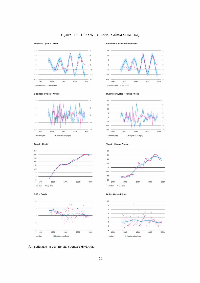
Figure D.9: Underlying model estimates for Italy

1940 1960 1980 2000 2020−15

−10

−5

0

5

10

15

−3

−2

−1

0

1

2

3

Financial Cycle − Credit

median (left) BIS (right)

1940 1960 1980 2000 2020−15

−10

−5

0

5

10

15

−3

−2

−1

0

1

2

3

Financial Cycle − House Prices

median (left) BIS (right)

1940 1960 1980 2000 2020−10

−5

0

5

10

−4

−2

0

2

4

Business Cycles − Credit

median (left) HP cycle GDP (right)

1940 1960 1980 2000 2020−15

−10

−5

0

5

10

15

20

−6

−4

−2

0

2

4

6

8

Business Cycles − House Prices

median (left) HP cycle GDP (right)

1940 1960 1980 2000 2020−50

0

50

100

150

200

250

300

350

Trend − Credit

●

●●●●●

●●●●●●●

●●●●●●●●●

●●●●●●●●●●●●

●●●●

●●●●●●

●●●●

●●●●●

●●●●●

●●●●

●●●●

●●●●

●●●●●●

●●●●●●●●●●●

●●●●●●●●●●

●●●●

●●●●

●●●●●●●●

●●●●●●

●●●●●●

●●●

●

●●●●

●●●●

●●●●

●●●●

●●●●

●●●●●●●●

●●●●

●●●●●●●●●●●●●●●●

●●●●

●●●●●●

●●●●●●

●●●●●●●

●●●

●●●●

●●●●

●●●●●●●

●●●●●●●●●●●●●●●●●●●●●●●●●●●●●●●●●●●●

●median Log data

1940 1960 1980 2000 2020−60

−40

−20

0

20

40

60

80

Trend − House Prices

●

●●

●●

●●●●●

●●●●●●●

●●●●

●●●●●

●●●●

●

●●

●

●●●

●

●●●●●●●●●

●●●●●

●

●

●

●●●●●●●●

●●●

●●●●●

●●●●

●

●

●

●

●●●●●

●●●●●●●●●●●

●

●

●●●●●●

●

●

●

●●●

●●●

●●●●

●●

●●●●

●●●

●●●●●●●●●

●

●

●●●

●

●●●

●●

●

●●●

●

●

●●●●●●

●●●●

●

●●●●●●●●

●●●●●●●●●●●●●●

●●●●●●

●●●●

●●●●●

●●●●●●●●

●●●

●●●●●●●

●●●●●●●●●

●●●●●●●●●●

●●●●●

●●●●●●●●●●●●●

●median Log data

1940 1960 1980 2000 2020−10

−5

0

5

10

Drift − Credit

●●

●●

●●

●●

●●●

●

●

●

●

●

●

●

●●

●

●●

●

●

●●●

●

●●●

●

●

●

●

●

●

●

●

●

●

●

●●

●●●

●

●

●

●

●

●●●

●

●●●●

●

●●

●

●●

●●●

●

●

●●●

●

●

●

●

●

●

●●

●

●

●

●

●

●●

●

●

●

●

●

●

●

●

●

●

●

●

●

●

●

●

●

●

●

●

●

●

●

●

●●

●

●

●

●

●

●

●

●

●

●

●

●

●

●

●

●

●

●

●

●

●

●

●

●

●

●

●

●

●

●

●

●

●

●

●

●

●

●

●

●

●

●

●

●

●

●

●

●

●

●

●

●

●

●

●

●

●

●

●

●

●

●

●

●

●

●

●

●

●

●●

●

●

●

●

●

●

●

●

●

●

●

●

●

●

●

●

●

●

●

●

●

●

●

●

●

●●

●●●

●

●

●

●

●

●●●

●

●

●

●●

●●

●

●

●●●●●●

●

●

●

●

●

●

●

●

●

●●

●

●

●median Mutations Log Data

1940 1960 1980 2000 2020−4

−2

0

2

4

6

8

10

Drift − House Prices

●

●

●

●

●

●

●

●

●

●

●●

●

●

●

●

●

●●

●

●●

●

●

●

●

●

●

●

●

●

●

●

●

●

●

●

●

●

●

●●

●

●

●

●

●

●

●●

●

●

●

●●

●

●

●

●

●

●

●●

●

●

●

●●

●●

●

●

●

●

●

●

●

●

●

●

●

●

●

●

●

●

●

●

●

●

●

●●

●

●

●

●

●

●

●

●

●

●

●

●

●●

●

●

●

●

●●●

●

●

●

●

●

●

●

●

●

●

●

●

●●

●

●

●●

●

●

●

●

●●

●

●

●

●

●

●

●

●

●

●

●

●

●

●

●●

●

●

●●●

●

●

●

●

●

●●

●

●

●

●

●●●

●

●

●

●

●

●

●●

●

●

●

●●●

●●

●

●

●

●

●

●

●

●●

●

●

●●●●

●●

●●

●●

●

●

●●

●

●

●

●

●

●

●

●

●●

●

●

●

●

●●

●

●●

●

●

●

●

●

●

●

●

●

●

●

●

●●●

●●

●

●

●

●median Mutations Log Data

All con�dence bands are one standard deviation.

44

Figure D.10: Underlying model estimates for Japan

1940 1960 1980 2000 2020−3

−2

−1

0

1

2

3

−3

−2

−1

0

1

2

3

Financial Cycle − Credit

median (left) BIS (right)

1940 1960 1980 2000 2020−15

−10

−5

0

5

10

15

−3

−2

−1

0

1

2

3

Financial Cycle − House Prices

median (left) BIS (right)

1940 1960 1980 2000 2020−20

−15

−10

−5

0

5

10

15

20

−8

−6

−4

−2

0

2

4

6

8

Business Cycles − Credit

median (left) HP cycle GDP (right)

1940 1960 1980 2000 2020−20

−10

0

10

20

−10

−5

0

5

10

Business Cycles − House Prices

median (left) HP cycle GDP (right)

1940 1960 1980 2000 20200

200

400

600

800

1000

Trend − Credit

●

●

●

●● ●

●

●

●●

●●

●

●

●●●●●

●●●●●●

●●●●●●

●●●●●●●●

●●●●●●●

●●●●●●●●●●●●●●●●

●●●●●●●●●●●●

●●●●●●●●●●●●●

●●●●●●●●●

●●●●●●●●

●●●●●●●

●●●●●●●●●

●●●●●●●●●●●●●●●●●●●●●●●●●●●●●●●●●●●●●●●●●●●●●●●●●●●●●●●●●●●●●●●●●●●●●●●●●●●●●●●●●●●●●●●●●●●●●●●●●●●●●●●●●●●

●

●median Log data

1940 1960 1980 2000 2020−400

−300

−200

−100

0

100

Trend − House Prices

●

●

●

●

●

●●●●

●●●●●●●●●●●●●●●●●●●●

●●●●●

●●●●●●

●●●

●●●●●●●●●●

●●●●●

●●●

●●●●

●●●●

●●●●

●●●●

●●●●●●●●

●●●●●●●●●●●●●●●●

●●●●●●●

●●●●●

●●●●●●●●●●●●●●●●●

●●●●●

●●●●●●

●●●●●●

●●●●●●●●●●●●●●●●●●●●●●●●●●●●●●●●●●●●●●●●●●●●●●●●●●●●●●●●●●●●●●●●●●●●●●●●●●●●●●●●●●●●●●●●●●●●●●●●●●●●●●●

●●●●●●●●

●median Log data

1940 1960 1980 2000 2020−10

−5

0

5

10

Drift − Credit

●

●

●

●

●

●

●●

●●

●

●

●

●

●

●●

●

●

●

●

●●

●

●

●

●

●

●

●

●

●

●

●

●

●

●●

●

●●

●

●

●●

●

●

●●●

●

●

●

●

●●●

●

●

●●

●

●

●

●

●

●

●

●

●

●

●

●

●

●

●

●

●

●

●

●

●

●

●

●

●

●

●

●

●

●

●●

●●●

●

●

●

●

●

●

●

●

●

●

●

●●

●

●

●

●

●

●

●

●

●●

●●

●●

●

●

●

●

●

●

●

●

●

●

●●

●

●

●

●

●

●

●

●

●

●

●

●

●

●

●

●

●●

●

●

●

●

●●

●

●

●

●

●

●●

●

●

●

●

●

●●

●

●

●

●

●

●

●

●

●

●

●

●

●●

●

●

●

●

●●●

●

●●

●●●

●

●●

●

●

●

●

●

●

●

●●

●

●

●

●

●

●

●

●●

●●●

●

●

●

●median Mutations Log Data

1940 1960 1980 2000 2020−10

−5

0

5

10

15

Drift − House Prices

●

●

●

●

●

●●

●

●

●

●

●

●

●

●●

●

●

●

●●

●●●

●

●

●

●

●

●●

●

●

●

●

●

●●

●

●

●

●

●

●

●

●

●●●

●

●●

●

●

●

●●

●

●

●

●

●

●

●

●

●

●

●

●

●

●

●

●

●

●●

●

●●

●

●

●

●

●

●

●

●●

●

●

●

●

●●●

●

●

●

●

●

●

●

●

●●

●

●

●

●

●

●

●●●

●

●

●

●

●●●

●

●

●

●●●

●●●●●

●

●

●●

●

●

●●

●●

●

●

●

●●●

●●

●

●

●

●

●

●●●●●

●

●

●●

●●

●●

●

●

●●●●

●

●

●

●●●

●

●

●●

●

●●●●

●

●●●●

●

●●●

●●

●

●●●

●●●

●

●●●●

●●

●●●●

●

●

●

●●

●

●

●

●

●

●●

●

●

●

●●

●●

●●

●

●

●

●

●●

●

●

●

●

●

●

●

●

●

●

●

●

●median Mutations Log Data

All con�dence bands are one standard deviation.

45

Figure D.11: Underlying model estimates for the Netherlands

1900 1920 1940 1960 1980 2000 2020−4

−2

0

2

4

6

−2

−1

0

1

2

3

Financial Cycle − Credit

median (left) BIS (right)

1900 1920 1940 1960 1980 2000 2020−30

−20

−10

0

10

20

30

40

−3

−2

−1

0

1

2

3

4

Financial Cycle − House Prices

median (left) BIS (right)

1900 1920 1940 1960 1980 2000 2020−40

−30

−20

−10

0

10

20

30

40

−8

−6

−4

−2

0

2

4

6

8

Business Cycles − Credit

median (left) HP cycle GDP (right)

1900 1920 1940 1960 1980 2000 2020−40

−30

−20

−10

0

10

20

30

40

−8

−6

−4

−2

0

2

4

6

8

Business Cycles − House Prices

median (left) HP cycle GDP (right)

1900 1920 1940 1960 1980 2000 2020−300

−200

−100

0

100

200

300

Trend − Credit

●●

●●

●

●● ● ●

● ●● ●

● ● ●●

● ●

● ● ● ●● ●

●

●● ● ● ●

●● ●

● ● ●●

●●

●

●

●

●

●●

●●

●●

● ●●

●

●

●

● ● ●

●

●●●●●●●●●●●

●●●●●●●●●

●●●●●●●●●●●●●●●

●●●●●●●●

●●●●●●●●●●●●●●●●●

●●●●●●●●●●●●●●●●●●●●●●●●●●●●●●●●

●●●●●●●●●●●●●●●●●

●●●●●●●●●

●●●●●●●●

●●●●●●●●●●

●●●●●●●●●

●●●●●

●●●●●●●●●

●●●●●●●●●●●●

●●●●●●●●●●●●●

●●●●●●●●●●●●

●●●●●●●●●●●●●●●●●●●●●●●●●●●●●●●●●

●median Log data

1900 1920 1940 1960 1980 2000 2020−100

−50

0

50

100

150

Trend − House Prices

●●

●●

●●

●●

● ●●

●●

● ●

●

●

●●

●

●●

●●

●● ●

●●

●

●

●

●

●

●

●

● ● ●

●

●

● ●

●

●

●

●

●

●

●

●

●●

●●

●

●●

●

●

●

●

●● ●

●

● ● ●

●

●●●●●●●

●●●●●●●●●●●●●●●●●●

●

●

●

●

●●●●

●

●●●●

●●●●

●●●

●

●

●

●●●●●●●●●●●

●●●●●●●●●●●●●●

●●●●●●●●

●

●●●●●●●●

●●●●●●●●●●●●

●●●●●●●●●●●●●●●

●

●

●●●●●●●●●●●●

●●●●●●●●

●●●●●●●

●●●●●●●●●●

●●●●●●●●●●●●

●●

●●

●●●●●●●

●●●●●●●●

●●●●●

●median Log data

1900 1920 1940 1960 1980 2000 2020−10

−5

0

5

10

Drift − Credit

●

● ●

●

●

●

●

●

●

●

●

●

●

●

●

●

●

●

●

●

●●

●

●

●

●

● ● ●

●

●

●

●

●

●

●

●

●

●

●

●

●

●

●

●

●

●

● ●

●

●

●

●●

● ●

●●

●

●

●

●

●●

●

●

●

●

●

●

●

●

●●

●

●●

●

●

●

●

●

●●●

●●

●

●

●

●

●

●

●●

●

●

●

●

●

●

●

●

●

●

●

●●

●●

●

●

●

●

●

●

●

●

●

●

●

●●

●●

●

●

●

●

●

●

●

●

●

●

●

●

●

●

●

●

●

●

●●

●

●●

●

●●

●

●

●

●

●

●

●

●

●

●

●

●

●

●

●

●

●●

●

●

●

●

●

●

●

●

●

●

●

●

●

●

●

●●

●

●

●●

●

●

●

●

●

●

●

●

●

●

●

●

●

●

●●

●

●

●

●●●●●●

●

●

●

●

●

●

●

●

●

●

●

●

●

●

●

●

●

●

●

●

●

●

●

●

●

●

●●

●

●●

●

●

●

●

●

●

●

●

●

●

●

●

●

●

●

●

●

●

●

●

●

●

●

●

●

●

●

●

●

●●

●●

●●●

●

●●●

●●

●median Mutations Log Data

1900 1920 1940 1960 1980 2000 2020−10

−5

0

5

10

15

Drift − House Prices

●

●

●

●● ●

●●

●

●

● ●

●●

●

●

●

●

●

●

●

●

●

● ●

●

●●

●

●

●●

●

●

●

●

● ●

●

●●

●

●

●

●

●

● ●

●

●

●

●

●

●

●●

●

●

●

●●

●

●

●

● ●

● ●

●

●

●

●●

●

●

●

●●

●

●

●

●

●

●

●

●

●

●

●

●

●

●

●

●

●

●

●

●

●

●

●●

●

●

●

●

●

●

●●

●

●

●

●

●

●

●

●

●

●

●

●

●

●

●

●●●

●

●

●

●

●

●

●●

●

●

●

●

●●

●

●●

●

●

●●

●

●

●

●

●

●

●

●

●

●

●

●●

●

●

●●

●

●

●

●

●●●

●

●

●

●●

●

●

●

●

●

●

●

●

●●●

●●

●●

●

●

●●

●

●

●●

●

●

●

●

●

●

●

●

●

●

●

●

●

●

●

●

●

●

●

●

●

●

●

●

●●

●

●

●

●

●●

●●●●

●

●

●

●

●

●

●

●

●

●

●

●

●●

●●

●●●

●

●

●

●

●

●median Mutations Log Data

All con�dence bands are one standard deviation.

46

Figure D.12: Underlying model estimates for Norway

1900 1920 1940 1960 1980 2000 2020−40

−30

−20

−10

0

10

20

30

40

−4

−3

−2

−1

0

1

2

3

4

Financial Cycle − Credit

median (left) BIS (right)

1900 1920 1940 1960 1980 2000 2020−20

−15

−10

−5

0

5

10

15

20

25

−2,0

−1,5

−1,0

−0,5

0,0

0,5

1,0

1,5

2,0

2,5

Financial Cycle − House Prices

median (left) BIS (right)

1900 1920 1940 1960 1980 2000 2020−30

−20

−10

0

10

20

30

−6

−4

−2

0

2

4

6

Business Cycles − Credit

median (left) HP cycle GDP (right)

1900 1920 1940 1960 1980 2000 2020−30

−20

−10

0

10

20

30

40

−6

−4

−2

0

2

4

6

8

Business Cycles − House Prices

median (left) HP cycle GDP (right)

1900 1920 1940 1960 1980 2000 20200

100

200

300

400

500

Trend − Credit

● ● ●● ●

● ● ● ● ● ● ●●

●●

●

●

●

●

●●

●

●

●

●

● ●●

●●●●●●●●

●●●●●●●●●●●●●

●●●●●●●●●●●

●●●●●●●●●●●●●●

●●●●●●●●●

●●●●●●

●●●●●●●●

●●●●●●

●●●●●●●●●●

●●●●●●●●●●●●●●●

●●●●●●●●●●●●●●●●●●●●

●●●●●●●

●●●●●●●

●●●●●●●

●●●●●●●●●●●●●●●●●●●●●●●●●●●●

●●●●●●●●●●●●●

●●●●●●●●●

●●●●●●●

●●●●●●●●●●●●●●●●●●●

●●●●●●●●●●

●●●●●●●●●●●●●●●

●●●●●●●●●●●●●●●

●median Log data

1900 1920 1940 1960 1980 2000 2020−50

0

50

100

150

200

Trend − House Prices

●

●●

●● ●

● ●

●

●●

●

● ● ●

●

●

●● ●

●

●

● ●●

●

●●

●

●

●● ● ●

●

●● ●

●●

● ● ●●

●

●●●●●●●●

●

●●●●●●

●●

●●●●●

●●

●

●●●

●●●●

●●●●●●●●

●●●●●

●●●●

●●●●●●●

●●●●●●●

●

●

●

●●

●●●●●●

●●

●●

●●●●

●●●●●●●●●

●

●

●●●●●●●●

●●●●●●●●

●●●●

●●●●

●●●

●

●●●●

●●●●●●●●●●●

●●●●●●●●

●●●●

●●●

●●●

●

●●●●●●

●●●

●●●●

●●●●

●●●●●●●●

●●●●●●●●

●●●●

●median Log data

1900 1920 1940 1960 1980 2000 2020−10

−5

0

5

10

Drift − Credit

●

●

●

●

●

● ● ●

● ●

●

●

●

●

●

●

● ●

●

●

●

●

●

●

●

●

●

●

●●

●

●

●

●

●●

●

●

●

●

●●

●●

●

●●

●

●

●●

●

●●●●

●●

●

●

●

●

●

●

●

●

●

●

●

●

●

●

●

●

●

●

●

●

●

●

●

●

●●●●●

●

●

●

●

●

●

●

●●

●●●

●

●

●●

●

●

●

●

●

●

●

●●

●

●

●

●

●

●

●●

●

●

●

●

●

●

●

●

●

●

●

●

●

●

●●

●

●●

●

●

●

●

●

●

●

●

●

●

●

●

●

●●

●

●

●

●

●

●

●

●

●

●

●

●

●

●

●

●

●●

●

●

●

●

●

●

●

●

●

●

●

●

●

●

●

●

●●●

●

●

●

●

●

●

●

●

●

●

●

●

●

●

●

●

●

●

●

●

●

●

●

●

●

●

●

●

●

●

●

●

●

●

●

●●

●●

●

●●●

●

●

●●

●●

●●

●

●

●

●

●

●

●

●

●●

●

●

●

●

●●●●

●

●

●

●

●

●

●

●●

●

●

●●

●

●●

●

●

●

●

●

●

●

●

●median Mutations Log Data

1900 1920 1940 1960 1980 2000 2020−10

−5

0

5

10

Drift − House Prices

●

●

●

●●

●

●

●

●

●

●

●

●●

●

●

●

●

●

●

●

●

●

●

●

●

●

●

●

●

●

●●

●

●

●

●

●

●

●

●●

●

●

●

●

●●

●

●●

●

●●

●

●

●

●

●

●

●

●

●

●

●

●

●

●

●

●

●

●

●

●

●

●

●

●

●

●●

●

●

●

●

●●

●

●

●

●

●

●

●

●

●

●

●

●

●

●

●

●

●

●

●

●

●

●

●

●

●

●

●

●

●

●●

●

●

●

●

●

●

●

●

●●●

●

●●

●

●●

●

●

●

●●

●●

●

●

●

●

●●

●

●

●

●

●

●

●

●

●

●

●

●

●

●

●

●

●

●

●

●

●

●

●

●

●

●

●

●

●

●

●

●

●

●

●

●

●

●

●●

●

●

●

●

●

●

●

●

●

●

●

●

●●

●

●

●

●

●

●

●

●

●

●

●

●

●

●

●●

●●

●

●

●●

●

●

●

●

●

●

●

●

●

●

●

●

●median Mutations Log Data

All con�dence bands are one standard deviation.

47

Figure D.13: Underlying model estimates for South Korea

1940 1960 1980 2000 2020−10

−5

0

5

10

−4

−2

0

2

4

Financial Cycle − Credit

median (left) BIS (right)

1940 1960 1980 2000 2020−20

−10

0

10

20

30

−2

−1

0

1

2

3

Financial Cycle − House Prices

median (left) BIS (right)

1940 1960 1980 2000 2020−40

−30

−20

−10

0

10

20

30

40

−20

−15

−10

−5

0

5

10

15

20

Business Cycles − Credit

median (left) HP cycle GDP (right)

1940 1960 1980 2000 2020−40

−30

−20

−10

0

10

20

30

40

−20

−15

−10

−5

0

5

10

15

20

Business Cycles − House Prices

median (left) HP cycle GDP (right)

1940 1960 1980 2000 20200

200

400

600

800

1000

1200

Trend − Credit

●●●●●

●●●●●●●

●●●●●

●●●●●

●●●●●●●●●

●●●●●

●●●●●

●●●●●●

●●●●●●●●●

●●●●●

●●●●

●●●●●

●●●●●●

●●●●●●

●●●●●

●●●●

●●●●●●●●

●●●●●●●

●●●●●

●●●●

●●●●●●

●●●●●●

●●●●●●●

●●●●●●

●●●●●●●●●●●●●●●●●●●

●●●●●●●●●●●●●●●●●●●

●●●●●●●●

●●●●●●●●●●●●●●●●●●●●

●●●●●●●●●●●●●●●

●median Log data

1940 1960 1980 2000 2020−40

−20

0

20

40

60

80

100

Trend − House Prices

●

●●

●●

●

●

●

●

●

●

●

●

●

●●

●●●

●

●●

●

●

●

●●●●●

●

●

●

●

●

●

●

●●●●

●●●

●●●●

●●●

●●

●

●●

●

●●●

●

●●

●●●

●

●

●

●

●●

●●●●

●●●●

●●●●

●●●●●●

●

●

●

●

●●●●●●●●

●●

●●

●

●

●

●

●

●●

●●●

●●●●

●●●

●●●●

●●●●●●●●●

●●●●●●

●●●●●

●●●●●●●●●●●●

●●●●●●●●●●●●●

●median Log data

1940 1960 1980 2000 2020−10

−5

0

5

10

15

20

Drift − Credit

●

●

●

●

●

●●

●

●

●

●

●

●

●

●

●

●

●

●

●

●

●

●

●●

●

●

●

●

●

●

●

●

●

●●

●

●

●

●

●

●

●

●

●

●

●

●

●

●

●

●●

●

●

●

●

●

●

●●

●

●

●

●

●

●

●

●●

●

●

●

●

●

●

●

●

●

●

●

●

●

●

●

●

●

●

●

●

●

●

●

●

●

●

●

●●●

●

●

●

●

●

●

●●

●

●

●

●

●●

●●

●

●

●

●

●

●

●

●●

●

●

●

●

●

●

●

●

●

●

●

●

●●

●

●

●

●

●

●

●

●

●

●

●

●●●

●

●

●

●●

●●

●

●

●

●

●

●

●●

●

●

●

●

●

●

●

●

●

●

●

●●●

●●

●

●

●●

●

●

●

●

●

●●

●●

●

●●

●●

●

●●

●

●●

●●

●

●

●

●

●

●

●

●

●

●

●median Mutations Log Data

1940 1960 1980 2000 2020−10

−5

0

5

10

Drift − House Prices

●

●

●

●

●

●

●●

●

●

●

●

●

●

●

●

●

●

●

●

●

●●

●

●

●●

●

●

●

●

●

●

●

●●

●

●

●

●

●

●

●

●

●●

●

●●

●

●

●

●

●

●

●

●

●

●

●

●

●

●

●

●

●

●

●

●

●

●

●

●●

●

●

●●

●

●

●

●

●

●

●●

●●

●

●

●

●●

●

●

●●

●●

●

●

●

●

●

●

●●

●

●

●●

●

●

●●

●

●

●

●

●

●

●●

●

●

●

●

●

●

●

●

●

●

●

●

●

●●

●

●

●

●

●

●

●

●

●

●

●

●

●

●

●

●

●

●

●●

●

●

●●●

●●●

●

●

●

●

●

●median Mutations Log Data

All con�dence bands are one standard deviation.

48

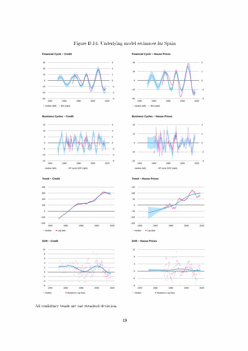
Figure D.14: Underlying model estimates for Spain

1940 1960 1980 2000 2020−30

−20

−10

0

10

20

30

−3

−2

−1

0

1

2

3

Financial Cycle − Credit

median (left) BIS (right)

1940 1960 1980 2000 2020−40

−20

0

20

40

−2

−1

0

1

2

Financial Cycle − House Prices

median (left) BIS (right)

1940 1960 1980 2000 2020−15

−10

−5

0

5

10

15

−6

−4

−2

0

2

4

6

Business Cycles − Credit

median (left) HP cycle GDP (right)

1940 1960 1980 2000 2020−20

−10

0

10

20

−4

−2

0

2

4

Business Cycles − House Prices

median (left) HP cycle GDP (right)

1940 1960 1980 2000 2020−200

−100

0

100

200

300

400

Trend − Credit

●●

●

●●

●

● ●● ●

●

●

●

●●

●

●●

●

●●●●●

●●●●●

●●●●

●●●●●●

●●●●●●●●●●●●●●●●●●●●●●●●

●●●●●●●●●●

●●●●●●●●●●●●●●●●●●

●●●●●●

●●●●●●●●

●●●●●●●●●●●●●●●

●●●●●●●●●●●

●●●●

●●●●

●●●●●

●●●●

●●●●●

●●●●

●●●●

●●●●●

●●●

●●●●●●●●●●●●●●●●●●●●●●

●●●●●●●●●●●●●●●●●●●●●

●median Log data

1940 1960 1980 2000 2020−150

−100

−50

0

50

100

150

Trend − House Prices

●●●●●●●●

●●●●

●

●●●●●

●●●●●●

●●●

●●●●●

●●●●●●

●●●●

●

●●●●●

●●●

●●●●●●●●●●

●●

●

●

●●

●●

●●●

●●●

●●●●●

●●●

●

●●●●

●●●●●●●●●●●●●●●●●●●●●

●●●●●●●

●●●●●●●

●●●●●

●

●●●

●●●●

●●●

●●●●●

●●●●●

●●●●●●●●●●

●●●●

●●●●●●●●●●●

●●●●●●

●●●●●●

●●

●median Log data

1940 1960 1980 2000 2020−6

−4

−2

0

2

4

6

8

10

Drift − Credit

●

●

●

●

●

●

●

●

●

●

●

●●

●

●

●

●

●

●

●

●

●

●

●

●●

●●

●

●

●

●

●

●

●

●

●●●●

●

●

●

●

●

●

●

●

●

●

●

●

●

●

●

●

●

●

●

●

●

●

●

●

●

●

●

●

●

●●

●

●

●

●

●

●

●

●

●

●

●

●

●

●

●

●

●

●

●

●

●

●

●

●

●

●

●

●

●

●

●

●

●

●

●

●

●

●

●

●

●

●

●

●

●

●

●

●

●

●

●

●

●

●

●

●

●

●

●

●●

●

●

●

●

●

●

●

●

●

●

●

●

●

●

●

●

●

●●

●

●●

●

●

●

●

●

●●

●

●

●

●

●

●

●●

●

●

●

●

●

●●

●

●

●

●

●●

●

●●

●

●

●

●

●

●

●

●

●

●

●

●

●

●

●

●

●

●

●

●

●

●

●

●

●

●

●median Mutations Log Data

1940 1960 1980 2000 2020−8

−4

0

4

8

12

Drift − House Prices

●

●

●

●

●

●

●

●

●

●

●

●

●

●

●

●

●

●

●

●

●

●

●

●

●

●

●

●

●

●●

●

●

●

●

●

●

●

●

●

●

●

●

●

●

●●

●

●

●

●

●

●

●

●

●

●

●●

●

●

●

●

●

●

●

●

●

●

●

●

●

●

●●

●

●

●

●

●

●

●

●

●

●●

●

●

●

●●

●

●●

●

●

●

●

●

●

●

●●●

●

●

●●

●

●

●●

●

●

●

●

●

●

●

●

●

●

●

●

●

●

●

●

●

●

●

●

●

●

●

●

●

●●

●

●

●

●

●

●

●

●

●

●

●

●

●●

●

●

●

●

●

●

●

●

●

●

●

●

●

●

●

●

●

●

●●●

●●

●●

●

●

●

●

●

●

●

●

●

●median Mutations Log Data

All con�dence bands are one standard deviation.

49

Figure D.15: Underlying model estimates for Sweden

1900 1920 1940 1960 1980 2000 2020−20

−15

−10

−5

0

5

10

15

20

−2,0

−1,5

−1,0

−0,5

0,0

0,5

1,0

1,5

2,0

Financial Cycle − Credit

median (left) BIS (right)

1900 1920 1940 1960 1980 2000 2020−20

−15

−10

−5

0

5

10

15

20

−2,0

−1,5

−1,0

−0,5

0,0

0,5

1,0

1,5

2,0

Financial Cycle − House Prices

median (left) BIS (right)

1900 1920 1940 1960 1980 2000 2020−10

−5

0

5

10

15

−5,0

−2,5

0,0

2,5

5,0

7,5

Business Cycles − Credit

median (left) HP cycle GDP (right)

1900 1920 1940 1960 1980 2000 2020−30

−20

−10

0

10

20

30

−6

−4

−2

0

2

4

6

Business Cycles − House Prices

median (left) HP cycle GDP (right)

1900 1920 1940 1960 1980 2000 20200

100

200

300

400

500

Trend − Credit

● ●●

● ● ● ● ●●

●●

●● ● ● ● ●

●●

●

● ●●

●

●

●● ● ●

●● ●

●

●● ●

●●

●●●●

●●●●●●●●●●

●●●●●●●●●

●●●●●●●●●●●●●●●●●●●●●●●

●●●●●●●●●

●●●●●●●●●●●●●●●●●●

●●●●●●●●●●●●●●●●●

●●●●●●●●●●

●●●●●●●●●●●●●●●●●●●●

●●●●●●●●●●●●●●●●●●●●●●●●●●●●●●

●●●●●●●

●●●●●●●●

●●●●●●●●●●●●

●●●●●●●

●●●●●●●●●●●●●

●●●●●●●●●●●

●●●●●●

●●●●●●●

●●●●●●●●●

●median Log data

1900 1920 1940 1960 1980 2000 2020−50

0

50

100

150

200

Trend − House Prices

●

●

● ●

●

●●

●●

●

● ●●

●●

● ● ● ●

●

●

● ●

●●

● ●

●

●

●

●

●

●

●●

●

● ●● ●

● ●

●

●●

●●

●●

●●●●●●●●●

●●●●●●●

●●●●

●●●●●●

●●●●

●●●

●●●●●●●

●●●

●●●●●●●●

●●●●●●●●●●●●●●

●●●●●●●●●

●●●●●●●●●

●●●●●

●●

●

●

●●●●●●●●●●●●●●

●●●●●●

●●●●●●●●●

●●●●●●●●

●●●●

●●●●●●●●●●●●●●●●

●●

●●●●●●●●●●●●●●●●

●●●●●

●●●●●●●●●●●●●●●●●●●●

●median Log data

1900 1920 1940 1960 1980 2000 2020−6

−4

−2

0

2

4

6

8

Drift − Credit

●

●

●

●

●

●

●●

●

●

●●

●

●●

●

●●

●

●

●

●

●

●

●

●

●

●

●

●

●

●

●

●

●

●

●

●

●

●

●

●

●

●

●

●●

●

●

●

●

●

●

●

●

●

●

●

●●

●

●

●

●

●

●

●

●●

●●●

●

●

●

●

●

●

●

●

●

●

●

●

●

●

●

●

●

●

●

●

●

●

●

●

●

●

●

●

●

●

●

●

●●

●

●

●

●

●

●

●

●

●

●

●

●

●

●

●

●

●

●

●●

●

●

●●

●

●

●

●

●●

●

●

●

●

●

●

●

●

●

●

●●●●●

●

●

●

●

●

●

●

●

●

●

●

●

●

●

●

●

●

●

●

●

●

●

●

●

●

●●

●

●

●

●

●

●

●

●

●

●

●

●

●●

●

●

●

●

●

●

●

●

●●

●

●

●●

●

●

●

●

●

●

●

●

●

●

●

●

●

●

●

●

●●

●

●

●●

●

●

●

●

●●

●

●

●

●

●

●

●●●

●

●

●

●

●

●

●

●

●

●

●

●●

●●

●

●

●

●

●

●

●

●●

●median Mutations Log Data

1900 1920 1940 1960 1980 2000 2020−10

−5

0

5

10

Drift − House Prices

●●

●

● ●

●●

●

●

●

●●

●

●

●

●

●

●

●

●

●

●

●

●

●

●

●

●

●

●

●

●

●

●

● ●

●

●●

●

●

● ●

●●

●

●

●

●

●

●

●

●

●

●

●●

●

●

●●

●

●

●

●

●

●

●

●

●

●●

●

●

●

●

●

●

●●

●

●

●

●

●

●

●

●

●

●

●

●

●

●

●

●●

●

●

●

●

●

●

●

●

●

●

●

●

●

●

●

●

●

●

●

●

●

●

●●

●

●

●

●

●●

●

●

●

●

●

●

●

●

●

●

●

●

●

●

●

●

●

●

●

●

●

●

●

●●

●

●

●

●

●

●

●

●

●

●●

●

●

●

●

●

●

●

●

●

●

●

●

●

●

●

●

●

●

●

●

●

●

●

●

●

●

●●

●

●

●●

●

●

●

●

●

●

●

●

●

●●●

●

●

●●

●

●

●

●

●

●●

●●

●●

●●

●

●

●

●

●

●●

●●

●

●

●

●

●●

●

●median Mutations Log Data

All con�dence bands are one standard deviation.

50

Figure D.16: Underlying model estimates for Switzerland

1900 1920 1940 1960 1980 2000 2020−20

−10

0

10

20

−10

−5

0

5

10

Financial Cycle − Credit

median (left) BIS (right)

1900 1920 1940 1960 1980 2000 2020−20

−15

−10

−5

0

5

10

15

20

−4

−3

−2

−1

0

1

2

3

4

Financial Cycle − House Prices

median (left) BIS (right)

1900 1920 1940 1960 1980 2000 2020−10

−5

0

5

10

−10

−5

0

5

10

Business Cycles − Credit

median (left) HP cycle GDP (right)

1900 1920 1940 1960 1980 2000 2020−20

−10

0

10

20

−10

−5

0

5

10

Business Cycles − House Prices

median (left) HP cycle GDP (right)

1900 1920 1940 1960 1980 2000 2020−50

0

50

100

150

200

250

300

Trend − Credit

●

● ●●

●

●

●

●

●

●

●

● ● ●●

●

● ●●

●

●

●● ●

●

●●

●●●●●●●●

●●●●●●●●●

●●●●●●●●

●●●●●●●

●●●●●●●●

●●●●●●●●●●●●●●●●

●●●●●●●●

●●●●●●●

●●●●●●●●●●●●●●●

●●●●●●●●●

●●●●●●●●●●●●●

●●●●●●●

●●●●

●●●●●

●●●●●●●●●●●●

●●●●●●

●●●●●●

●●●●●●●●●●●●●●●●●

●●●●●●●●●●●●●●●●●●●●●●●●●●●●●

●●●●●●●●●●●

●●●●●●●●●●●●●

●●●●●●●●

●●●●●●●●●●●●●

●●●●●

●●●●●●●●●●●

●●●●●●●●●●

●●●●●

●●●●●●●

●median Log data

1900 1920 1940 1960 1980 2000 2020−80

−60

−40

−20

0

20

40

60

Trend − House Prices

●

●

●

●

●

● ●

●

●●

●

●●

●● ●

●●

●

●

●

● ●

●

●

●●

●

●

● ●

●

●

●

●

●

●●

●●

●

●●

●●

●

●

●

●

●●●●

●●

●●

●

●

●

●

●

●●

●●●●

●

●

●●●

●●●●●●

●●●●●

●●●

●

●

●

●●●●●●●●

●●●●●

●●●●●●

●●●●

●●●●●●●●

●

●

●

●●●●●●●

●

●●●●

●

●●

●●

●●

●●●●●

●●●●●●●●

●●●●●●●●●●●●●●●

●●●●●●

●●●●●●●●●●

●●●●

●●●●●●●●●●●●

●●

●●●●●●●●●●●

●●●●●●●●●●●

●●●●●●●●

●●●●●●

●median Log data

1900 1920 1940 1960 1980 2000 2020−6

−4

−2

0

2

4

6

Drift − Credit

●

●

●

●

●

●

●

●

● ●

●

● ●

● ●

●

●

●

●

●

●

●

●

●

●

●●

●

●●

●

●

●

●

●

●

●

●●

●

●●

●

●

●●

●

●

●

●

●

●

●●●

●

●

●●

●

●

●

●

●

●

●

●

●

●

●

●●

●●

●

●

●

●

●

●

●

●

●

●

●

●

●

●

●

●

●

●

●

●

●

●

●

●

●

●

●

●

●

●

●

●

●

●

●●

●

●

●

●

●

●

●

●

●

●

●

●

●

●

●

●

●

●

●

●

●

●

●

●

●

●

●

●

●

●

●

●

●

●

●

●

●

●

●●

●

●

●

●

●

●

●

●

●

●

●

●

●

●

●

●

●

●

●

●

●

●

●

●

●

●

●

●

●

●

●

●●

●

●

●

●

●

●

●

●

●

●

●

●

●

●

●●

●

●●

●

●

●

●

●

●

●

●

●

●

●

●

●

●

●

●

●●

●

●

●●

●

●

●

●

●

●

●

●

●

●●

●

●●

●

●

●

●

●

●

●

●

●●

●

●

●

●

●

●

●

●

●

●

●

●

●

●

●

●

●

●

●

●

●

●

●

●

●

●

●

●

●●

●

●

●●

●

●

●

●

●

●

●●●

●

●

●

●

●

●

●

●

●

●

●●

●median Mutations Log Data

1900 1920 1940 1960 1980 2000 2020−8

−6

−4

−2

0

2

4

6

Drift − House Prices

●

●

●●

●

●

●

●

●

●●

●

●

●

●

●

●

●

●

●

●

●

●

●

●

●

●

●

●

●

●●

●

●● ●

●

●

●

●

●

● ●

●

●

●

●●

●

●

●

●

●

●

●

●

●

●

●

●

●

●

●

●

●

●

●

●

●

●

●

●

●

●

●

●

●

●

●

●

●

●●

●

●

●

●

●

●

●

●

●

●●

●

●

●

●

●

●

●

●

●

●

●

●

●

●

●

●

●

●

●

●

●

●

●

●

●

●

●●

●●

●

●

●

●

●●

●

●

●

●

●

●

●

●

●

●

●

●

●

●

●

●

●

●

●

●

●

●

●

●●

●

●●

●

●

●

●

●

●

●

●

●

●

●

●

●

●

●

●

●

●

●

●

●

●

●●

●

●

●

●

●

●

●

●

●

●

●

●

●

●

●

●

●

●

●

●

●

●

●

●

●

●

●●

●

●

●

●

●

●

●

●

●

●

●

●

●●

●

●●●

●

●

●●

●

●

●

●

●●●

●

●median Mutations Log Data

All con�dence bands are one standard deviation.

51

Figure D.17: Underlying model estimates for the United Kingdom

1900 1920 1940 1960 1980 2000 2020−20

−10

0

10

20

−4

−2

0

2

4

Financial Cycle − Credit

median (left) BIS (right)

1900 1920 1940 1960 1980 2000 2020−30

−20

−10

0

10

20

30

−3

−2

−1

0

1

2

3

Financial Cycle − House Prices

median (left) BIS (right)

1900 1920 1940 1960 1980 2000 2020−20

−10

0

10

20

30

−4

−2

0

2

4

6

Business Cycles − Credit

median (left) HP cycle GDP (right)

1900 1920 1940 1960 1980 2000 2020−20

−10

0

10

20

30

−4

−2

0

2

4

6

Business Cycles − House Prices

median (left) HP cycle GDP (right)

1900 1920 1940 1960 1980 2000 2020−100

0

100

200

300

400

Trend − Credit

●●

●●

●●

●●

●●

●● ●

● ●●

●●

●

●

●●

● ●●

●

●●

●● ●

● ●● ● ● ●

●

●

● ●●●●●●

●●●●

●●●●●●

●●●●●●●

●●●●●●●●●●

●●●●●●●●●●

●●●●●●●●●●●●●●

●●●●

●●●●●

●●●●●●●●●●

●●●●●●●●●●●●●●●●

●●●●●●●●●●●●●●●●●●●●●●

●●●●●●●●●●●●●●●●●●●

●●●●●●●

●●●●●●●●●●●●●●●●●

●●●●●●

●●●●●●●●

●●●●●

●●●●●●●●●

●●●●●●●●●●●●●●●●●●●●●●●●●●●●●●

●●●●●●●

●median Log data

1900 1920 1940 1960 1980 2000 2020−150

−100

−50

0

50

100

150

Trend − House Prices

●

●

●●

●

● ●

●

●●

●

● ●● ● ●

●●

●

●

●● ●

●

●●

● ●

●● ● ●

●●

●● ●

● ●●●

●●●●●●●●●●●●

●●●

●

●

●

●●●●●

●●●●

●●●●●●

●●●●●●●●

●●●●●●●

●●●●●

●●●●●●●●●●●

●●●●●●●●●●●●●●●●

●●●●●●●●●●●●●●

●●●●●●●●●●

●●●●●●●●●●●●●●●●●●●

●

●●●●●●●●

●●●

●

●●●●●●●●●●●●●●●

●●●●●●●●●●

●

●●●●●●

●●●●●●●●●●●●

●●●●●●●●

●●●●●●●●

●●

●median Log data

1900 1920 1940 1960 1980 2000 2020−10

−5

0

5

10

15

Drift − Credit

●●

●

●

●

●

●●

●

●

●

●

●

●

●

●

●

●

●

●

● ●

●

●

● ●

● ●●

●

●

●

●

●

●

●

●

●

●

●

●

●

●

●

●

●

●

●

●

●

●

●

●●

●

●

●

●

●

●

●

●

●

●

●

●

●

●

●●

●

●

●

●

●

●

●

●

●

●

●●

●

●

●

●

●

●

●

●

●

●

●

●

●

●●

●

●

●

●

●●

●

●●●

●

●

●

●

●●

●

●

●

●

●

●

●●

●

●●

●

●

●

●

●

●

●

●

●

●

●●

●

●

●

●

●

●●●

●

●

●

●

●

●

●

●

●●

●

●

●

●

●

●

●

●●

●

●

●

●

●●

●●

●

●

●

●

●

●●

●

●

●

●●

●

●

●●

●

●

●●●

●

●

●

●

●

●●

●

●

●

●

●●●●

●

●

●

●

●●●

●

●

●●

●

●

●

●

●

●

●

●

●

●

●

●

●

●

●

●●●●

●●

●

●●

●

●●●●

●●

●

●

●

●

●●●

●

●

●●

●

●median Mutations Log Data

1900 1920 1940 1960 1980 2000 2020−10

−5

0

5

10

15

Drift − House Prices

●

●

●

●●

●

●

●

●

●

●

●

●

● ●

●

●

●

●

●

●●

●

●

●

●

●

●

● ●

●

●●

●

●

●

●

●

●

●

●

●

●

●

●●

●

●

●

●

●

●

●

●

●

●

●

●

●

●

●

●

●

●

●

●

●

●

●

●

●

●

●

●

●

●

●

●

●

●

●

●

●

●

●

●

●

●

●

●

●

●

●

●

●

●

●

●

●

●●

●

●

●

●

●

●

●

●

●

●

●●

●

●

●

●●

●

●

●●

●

●●●

●

●●

●

●

●●

●

●

●

●

●

●

●

●

●

●

●

●

●

●

●

●

●

●

●●●

●

●

●

●●

●

●

●

●

●

●

●

●

●

●

●

●

●

●

●

●

●

●

●

●●

●

●

●

●

●

●●

●

●

●●

●●

●●

●

●

●

●

●

●

●

●

●

●

●●

●

●

●●

●

●

●

●

●

●

●●

●

●

●●

●●

●

●

●●

●●

●

●

●●

●

●median Mutations Log Data

All con�dence bands are one standard deviation.

52

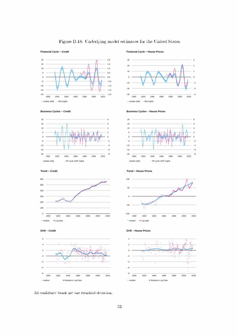
Figure D.18: Underlying model estimates for the United States

1900 1920 1940 1960 1980 2000 2020−20

−15

−10

−5

0

5

10

15

20

−2,0

−1,5

−1,0

−0,5

0,0

0,5

1,0

1,5

2,0

Financial Cycle − Credit

median (left) BIS (right)

1900 1920 1940 1960 1980 2000 2020−30

−20

−10

0

10

20

30

−3

−2

−1

0

1

2

3

Financial Cycle − House Prices

median (left) BIS (right)

1900 1920 1940 1960 1980 2000 2020−20

−15

−10

−5

0

5

10

15

20

−8

−6

−4

−2

0

2

4

6

8

Business Cycles − Credit

median (left) HP cycle GDP (right)

1900 1920 1940 1960 1980 2000 2020−20

−15

−10

−5

0

5

10

15

20

−8

−6

−4

−2

0

2

4

6

8

Business Cycles − House Prices

median (left) HP cycle GDP (right)

1900 1920 1940 1960 1980 2000 20200

100

200

300

400

500

600

Trend − Credit

● ● ● ●

●●

●● ●

●●

●●

●●

●● ●

●

●●

● ●● ●

●● ●

●

● ●●

●

●●

●

●●●●●●●●●●●

●●●●●●●●●

●●●●●●●●

●●●●●●●

●●●●●●●

●●●●●●

●●●●●●

●●●●●●●

●●●●●●●●

●●●●●●●●●●●

●●●●●●

●●●●●●●●●●●●●●●●●●

●●●●●●●●●●●●●●●●●●●●●

●●●●●●●●●●●

●●●●●●●

●●●●●●●●●

●●●●●●●●●●●●●●●●●●●●●●●●

●●●●●●●●●

●●●●●●

●●●●●●

●●●●●●●●●●

●●●●●●●●●●

●●●●●●

●●●●●●●●●●●●●●●●●●●●●●●●●●●●●●

●●●●●●●●●●●●●

●median Log data

1900 1920 1940 1960 1980 2000 2020−100

−50

0

50

100

Trend − House Prices

●

● ●

●

●●

●

●

● ●●

●● ●

● ●

●● ●

●

●

●● ●

● ●●

●

●

●

●

●

●

● ●●

● ●

●

●● ●

● ● ●● ● ● ● ● ● ●

●●

● ●●●●●

●●●●●●●●●●●●●●●

●●●●●

●●●●●●●●●●●●●●●●●

●●●●●●●●

●●●●●●●●●●

●●●●●●●●●●●●●●●●●●●●

●●●●●●●●●●●●●●●●●●●●●●●●●●●●●●●

●●●●●●●●●●●●●●●●●●●●●●●●●

●●●

●

●●●●

●●●●●

●

●●

●

●

●

●●

●●●●●●

●●●●●●●

●●●●●●●●●

●●●●

●●●●

●●●●●●

●median Log data

1900 1920 1940 1960 1980 2000 2020−6

−4

−2

0

2

4

6

Drift − Credit

●●

●

●

●

●

●

●

●

●

●

●

● ●

● ●

●

●

●

●

●

●

●

●

●

●

●

●

●

●

●

●

●

●

●

●

●

●●

●

●

●●

●●

●

●

●

●

●

●

●

●

●●

●

●

●

●

●

●

●

●

●

●

●

●

●

●

●

●

●●

●

●

●

●

●

●

●

●

●

●

●

●

●

●

●

●

●

●●

●

●

●

●

●

●

●

●

●

●

●

●

●

●

●

●

●

●

●

●●

●

●

●●

●

●

●

●

●

●

●

●

●

●

●

●

●

●

●

●●

●

●

●

●

●

●

●

●

●●●

●

●●

●

●●

●

●

●

●

●

●

●

●

●

●

●●

●

●

●

●

●

●

●

●●

●

●●●

●

●

●

●

●

●

●

●

●

●

●●

●

●

●

●

●

●

●

●

●

●

●●

●

●

●●●

●

●

●

●

●

●●

●

●

●

●●

●

●

●

●

●

●

●

●

●●

●●

●

●

●

●

●

●

●

●

●

●●

●

●

●

●

●

●

●

●

●

●

●

●

●

●●

●

●

●

●

●

●

●

●

●

●

●

●

●●

●

●

●

●

●

●

●

●

●

●

●

●

●

●

●

●

●

●

●

●

●

●

●

●

●

●

●

●

●

●

●

●

●median Mutations Log Data

1900 1920 1940 1960 1980 2000 2020−8

−6

−4

−2

0

2

4

Drift − House Prices

●

●

●

●

●

●

●

●

●

●

●

●

●

●

●

●

●

●

●●

●

●

●

●

●

●

●

●

●

●

●

●

●

●

●

●

●

●

●

●

●

●

● ●

●

●● ●

●

●

●

● ● ●

●

●

●

●

●

●

●

●

●

●

●

●

●

●

●●

●

●

●●

●

●●

●

●

●

●

●●

●

●●

●

●

●

●●

●

●●●

●

●

●

●●

●

●

●●

●

●

●

●

●

●

●

●●●

●

●

●●

●

●

●

●●

●●

●

●

●

●●

●

●

●

●●

●

●

●

●●

●

●●●●

●

●

●

●

●●

●

●

●

●

●

●

●●

●

●

●

●

●

●●

●

●●

●

●

●

●

●

●

●

●

●

●

●●

●

●

●

●●

●

●

●

●

●

●

●

●●

●

●

●

●

●

●

●

●

●

●

●

●

●

●

●

●

●

●

●●

●●

●

●

●

●

●

●

●

●

●

●

●

●

●

●

●●

●

●

●

●

●

●

●

●

●

●

●

●

●

●

●median Mutations Log Data

All con�dence bands are one standard deviation.

53

E Parameter posteriors

The posterior means and posterior standard deviations of the model parameters are shown below

in Tables E.1, E.2 and E.3.

54

Table E.1: Parameter Posterior of Measurement and Trend Error Covariances

" �

Country �"1 �"2 �h1 �h2 ��1 ��2

Australia 0.0056 0.0016 0.039 { 0.03 0.03

0.0011 0.0003 0.006 { 0.01 0.01

Belgium 0.0085 0.0065 0.036 0.155 0.04 0.03

0.0017 0.0010 0.006 0.025 0.01 0.01

Canada 0.0047 0.0105 0.096 0.194 0.03 0.03

0.0007 0.0035 0.016 0.031 0.01 0.01

Denmark 0.0028 0.0069 0.050 0.049 0.15 0.15

0.0004 0.0014 0.008 0.008 0.05 0.05

Finland 0.0012 0.0012 0.202 0.201 0.07 0.03

0.0002 0.0002 0.033 0.033 0.02 0.01

France 0.0005 0.0005 0.269 0.227 0.06 0.03

0.0001 0.0001 0.047 0.038 0.02 0.01

Germany 0.0020 0.0010 { 0.321 0.17 0.15

0.0004 0.0002 { 0.055 0.06 0.04

Ireland 0.020 0.021 { { 0.04 0.03

0.004 0.004 { { 0.01 0.01

Italy 0.009 0.009 { { 0.06 0.03

0.001 0.002 { { 0.02 0.01

Japan 0.0012 0.0002 0.273 0.223 0.010 0.009

0.0002 0.00004 0.048 0.037 0.003 0.003

Netherlands 0.006 0.007 0.255 0.204 0.010 0.010

0.001 0.001 0.043 0.033 0.003 0.003

Norway 0.004 0.004 0.250 0.187 0.010 0.010

0.001 0.001 0.041 0.030 0.003 0.003

South Korea 0.014 0.180 { { 0.010 0.010

0.004 0.004 { { 0.003 0.003

Spain 0.0020 0.37 0.049 { 0.05 0.02

0.0003 0.34 0.008 { 0.02 0.01

Sweden 0.003 0.004 0.271 0.199 0.018 0.015

0.001 0.001 0.046 0.032 0.006 0.005

Switzerland 0.002 0.003 0.088 0.098 0.010 0.013

0.000 0.001 0.014 0.016 0.003 0.004

UK 0.009 0.009 0.023 0.023 0.007 0.010

0.003 0.002 0.004 0.004 0.002 0.003

US 0.0009 0.0023 0.252 0.060 0.002 0.006

0.0002 0.0004 0.054 0.010 0.001 0.002

The table lists the posterior means and posterior standard deviations of the parameters. The �rst

row for each country shows the mean, while the value directly under is the standard deviation.

55

Table E.2: Parameter Posteriors of Drift and Seasonal Error Covariances

� !

Country ��1 ��2 ��12 �!1 �!2

Australia 0.0079 0.0066 0.0005 0.00003 0.00002

0.0012 0.0010 0.0008 0.00001 0.00001

Belgium 0.0077 0.0078 0.0011 0.00002 0.00002

0.0013 0.0013 0.0009 0.00001 0.00001

Canada 0.0087 0.0025 0.00003 0.00002 0.00002

0.0015 0.0004 0.0006 0.00001 0.00001

Denmark 0.0068 0.0077 0.0009 0.00002 0.00002

0.0011 0.0013 0.0008 0.00001 0.00001

Finland 0.0001 0.0000 0.0000 0.00002 0.00002

0.00002 0.0000 0.0000 0.00001 0.00001

France 0.0070 0.0099 0.0003 0.00005 0.00002

0.0011 0.0018 0.0010 0.00004 0.00001

Germany 0.0068 0.0075 0.0005 0.00003 0.00002

0.0011 0.0012 0.0008 0.00002 0.00001

Ireland 0.0077 0.0065 0.0004 0.00002 0.00002

0.0013 0.0011 0.0008 0.00001 0.00001

Italy 0.0072 0.0069 -0.0006 0.00454 0.00002

0.0012 0.0011 0.0008 0.00135 0.00001

Japan 0.0117 0.0124 0.0048 0.00002 0.00002

0.0019 0.0021 0.0016 0.00001 0.00001

Netherlands 0.0285 0.0082 0.0041 0.00002 0.00002

0.0055 0.0015 0.0022 0.00001 0.00001

Norway 0.0078 0.0067 -0.0001 0.00002 0.00002

0.0013 0.0011 0.0008 0.00001 0.00001

South Korea 0.0077 0.0018 0.0002 0.00002 0.00002

0.0012 0.0003 0.0004 0.00001 0.00001

Spain 0.0108 0.0065 0.0002 0.00004 0.00002

0.0020 0.0011 0.0011 0.00006 0.00001

Sweden 0.0064 0.0113 0.0001 0.00002 0.00002

0.0010 0.0018 0.0010 0.00001 0.00001

Switzerland 0.0089 0.0082 0.0015 0.00003 0.00002

0.0015 0.0015 0.0011 0.00001 0.00001

UK 0.0084 0.0069 -0.0011 0.00002 0.00002

0.0014 0.0012 0.0009 0.00001 0.00001

US 0.0115 0.0025 -0.0004 0.00002 0.00002

0.0023 0.0004 0.0007 0.00001 0.00001

The table lists the posterior means and posterior standard deviations of the parameters. The �rst

row for each country shows the mean, while the value directly under is the standard deviation.

56

Table E.3: Parameter Posteriors of Cycle Components

F� B

�

Country �F�1 �F�2 �B�1 �B�2 �B�12 �F �B �F �B

Australia 0.01 0.92 1.82 1.91 0.23 68.6 25.5 0.989 0.9600.02 0.30 0.17 0.33 0.16 3.7 1.8 0.004 0.010

Belgium 1.51 0.50 3.79 2.72 0.15 71.8 36.6 0.994 0.9630.66 0.23 0.63 0.41 0.14 2.7 3.2 0.002 0.010

Canada 0.17 4.96 2.19 0.09 0.07 72.5 30.0 0.988 0.9640.10 0.49 0.22 0.04 0.06 4.9 2.5 0.004 0.009

Denmark 1.14 0.01 0.24 5.85 0.48 71.1 37.8 0.991 0.9730.18 0.003 0.09 0.61 0.18 3.4 2.7 0.003 0.008

Finland 0.40 0.30 2.27 3.91 0.20 74.5 40.2 0.995 0.9770.30 0.15 0.37 0.46 0.16 2.2 2.4 0.002 0.006

France 0.03 0.30 0.71 0.28 0.04 64.7 28.4 0.994 0.9740.02 0.07 0.10 0.06 0.03 3.3 1.8 0.002 0.007

Germany 0.15 0.23 0.36 0.24 0.06 70.1 37.4 0.989 0.9680.10 0.07 0.09 0.06 0.05 4.5 3.8 0.004 0.011

Ireland 0.40 3.47 12.6 3.11 0.29 76.3 36.4 0.993 0.9710.33 0.90 1.39 0.82 0.27 3.5 2.8 0.003 0.009

Italy 0.17 0.25 1.21 1.64 0.08 69.2 34.9 0.995 0.9700.06 0.15 0.15 0.21 0.06 2.8 2.5 0.002 0.008

Japan 0.02 0.29 0.83 1.16 0.57 62.6 26.6 0.991 0.9780.01 0.13 0.09 0.16 0.09 4.5 1.3 0.003 0.005

Netherlands 0.06 1.48 2.47 3.80 0.57 72.7 41.3 0.993 0.9790.17 0.68 0.27 0.80 0.27 4.2 2.9 0.003 0.005

Norway 0.66 0.38 1.43 6.39 0.14 77.5 41.9 0.996 0.9800.19 0.23 0.21 0.65 0.12 2.2 2.1 0.001 0.005

South Korea 0.24 0.67 5.29 2.56 1.09 77.4 36.4 0.993 0.9840.42 0.43 0.65 0.54 0.52 4.4 2.7 0.003 0.005

Spain 0.65 1.68 1.87 2.65 0.15 69.0 36.2 0.993 0.9710.36 0.48 0.32 0.54 0.13 3.2 3.0 0.002 0.009

Sweden 0.93 0.61 1.55 4.09 0.18 69.1 35.0 0.991 0.9630.26 0.34 0.27 0.54 0.15 3.2 3.5 0.003 0.010

Switzerland 0.47 0.38 0.78 1.99 0.20 72.3 36.2 0.993 0.9680.21 0.19 0.17 0.26 0.13 3.8 2.3 0.002 0.007

UK 0.63 1.30 4.09 3.24 0.68 71.9 34.9 0.993 0.9650.37 0.36 0.51 0.49 0.38 2.3 2.8 0.002 0.008

US 0.13 0.67 0.65 0.72 0.05 77.7 34.7 0.996 0.9860.05 0.14 0.07 0.13 0.04 2.3 1.3 0.002 0.004

The table lists the posterior means and posterior standard deviations of the parameters. The�rst row for each country shows the mean, while the value directly under is the standarddeviation.

57