Human Capital Risk in Life-cycle Economies

Aarti Singh�

April 2008 †

AbstractI study the effect of market incompleteness on the aggregate econ-

omy in a model where agents face idiosyncratic, uninsurable humancapital investment risk. The environment is a general equilibrium life-cycle model with a version of a Ben-Porath (1967) human capital accu-mulation technology, modified to incorporate risk. A CARA-normalspecification keeps endogenous decisions independent of individualshock realizations. I study stationary equilibria of calibrated cases inwhich idiosyncratic uninsurable risk arises from specialization risk andcareer risk. Specialization risk is such that both mean and varianceof the return from training are increasing in the endogenous decisionto invest in human capital. In the case of career risk, however, onlythe mean return is increasing in the decision to invest in human cap-ital. With career risk only, stationary equilibria resemble those stud-ied by Aiyagari (1994), and one concludes that the impact of uninsur-able idiosyncratic risk is relatively small. With a significant amountof specialization risk however, stationary equilibria are severely dis-torted relative to a complete markets benchmark. One aspect of thisdistortion is that human capital is only about 57 percent as large asits complete markets counterpart. This suggests that the two types ofrisk have very different and quantitatively significant general equilib-rium implications. Keywords: Human capital risk, life-cycle, incom-plete markets. JEL codes: E20, E21, E24.

�Department of Economics, University of Sydney; a.singh@econ.usyd.edu.au.†I especially thank James Bullard for very valuable discussions and suggestions. I also

thank George-Marios Angeletos, Costas Azariadis, Riccardo Dicecio, Carlos Garriga, AlbertMarcet, James Morley, Suraj Prasad and Steve Williamson for their helpful comments andsuggestions. I also thank workshop and seminar participants at the FRB-St. Louis, Washing-ton University, University of New Orleans, University of Sydney, Unversity of New SouthWales, FRB-New York, SUNY-Stony Brook, Macro Reading Group–Washington Universityfor their comments on an earlier draft. All errors are my own.

1 Introduction

1.1 Human capital risk

Dispersion of labor earnings increases over the life-cycle, a well documented

feature of the US data. According to Deaton and Paxson (1994), within-

cohort labor income inequality increases with age. In related work, Huggett

Ventura and Yaron (2007) investigate the reasons behind this rise in earn-

ings dispersion over the life-cycle which is primarily due to age effects in

a partial equilibrium framework. Their study finds that about one-third

of the variation in lifetime earnings is due to idiosyncratic human capi-

tal shocks. Other cross sectional studies also indicate that agents face a

great deal of uncertainty when making their schooling decisions.1 Taken

together, it appears that investment in human capital is risky and part of

the labor income uncertainty that agents face over their life-cycle is a man-

ifestation of this idiosyncratic human capital risk. In addition, it is widely

understood that human capital investment is uninsurable—there is a clear

lack of complete markets with respect to this investment.

One main consequence of this type of labor income uncertainty is that

it could deter investment in human capital, possibly leading to underac-

cumulation of human capital and overaccumulation of relatively less risky

physical capital, in comparison to a case where agents can insure against

this risk via complete markets. If a mechanism like this is at work in actual

economies, the impact of market incompleteness on the aggregate econ-

omy could be large,2 possibly calling for policy intervention to mitigate the

1Carneiro, Hansen and Heckman (2003) find that the substantial heterogeneity in thereturns to schooling is unpredictable at the time when schooling decisions are made. Inrelated work, Cunha, Heckman, and Navaro (2005) conclude that 40% of the variabilityin the returns to schooling is unforecastable at the time students decide to go to college,implying that this uncertainty is not due to observable factors like ability differences ordifferences in initial conditions but purely due to idiosyncratic shocks.

2Even more so if one takes the view that human capital is an engine of growth. With theexception of few, Levhari and Weiss (1974), Eaton and Rosen (1980), Krebs (2003), Benabou(2002), for example, this strand of the literature typically abstracts from the risky nature ofhuman capital investment.

1

effect of this risk on household decisions to invest in training.3

I study the macroeconomic implications of labor income uncertainty

arising from the risky nature of human capital investment. The specifica-

tion here allows a direct analysis of the impact of risk on the process of

human capital accumulation, isolate and quantify the effect of risk on indi-

vidual decisions, and comment on divergent views in this literature on the

role of market incompleteness on the aggregate economy.

1.2 Main ideas

In this paper, investment in human capital is studied as a time allocation

problem in a life-cycle framework. Here agents allocate time away from the

labor market when they are young to acquire education. Using a version of

a Ben-Porath (1967) production function for human capital that allows for

risky human capital, I study how uninsurable risk impacts an individual’s

decision to train in a general equilibrium life-cycle model.4 If the returns

to training are uncertain and uninsurable, agents may try to self-insure by

holding larger precautionary savings and, more importantly, they may also

endogenously alter their training decisions to mitigate the effect of human

capital risk.

I consider two types of uninsurable idiosyncratic risks, namely, spe-

cialization risk and career risk. Higher risk is compensated by higher re-

turn, and higher return is often associated with higher levels of education.

In the formulation of the returns from training, this aspect of education

is captured by the specialization risk. The specialization risk is such that

the endogenous decision to train increases both the expected returns from

training and its variance, while the career risk only affects the mean return

3Krebs (2003) comes to this conclusion in an endogenous growth model where invest-ment in risky human capital is modeled as a portfolio decision and physical capital is therisk-free asset.

4I abstract from the risks associated with physical capital investment. Underlying thisassumption is the notion that for an individual human capital investment is more riskythan investment in physical capital. Typically investment in human capital cannot be easilydiversified or directly traded in the market since it is non-separable from the owner.

2

from training. The career risk is additive in the human capital accumu-

lation technology and is the most common formulation in the literature

which studies the impact of uninsurable idiosyncratic risk on the aggre-

gate economy. Risks that look like the multiplicative specialization risk of

this paper were first studied by Angeletos and Calvet (2006), but not in a

human capital setting.

Market incompleteness arising because of these idiosyncratic uninsur-

able risks make the wealth distribution a relevant state for individual de-

cisions, often making problems in this class intractable. Several papers,

including Calvet (2001) and Angeletos and Calvet (2006), use constant ab-

solute risk aversion (CARA) utility function and normally distributed shocks

in order to ensure that an individual’s risk-taking decision is independent

of wealth. I employ the same technique along with certain other assump-

tions to ensure that an individual’s decisions are independent of wealth.

Due to the lack of wealth effects, within a generation all agents make iden-

tical decisions but they still differ in their labor quality, labor income, and

consumption because of the different realizations of the two shocks. In the

life-cycle model that I consider, therefore, there are both types of hetero-

geneity, within generation and across generation. Across generation het-

erogeneity is inherent in the life-cycle models.

I study calibrated versions of the model to assess the quantitative im-

portance of incomplete markets. Risk related parameters—the variances of

the two shock processes in the human capital accumulation technology—

are chosen to match the portion of the variance in labor earnings over the

life-cycle that is due to age effects. I study a baseline case which has a mix-

ture of the two types of shocks, and also a more extreme case where there

is only career risk. Such an analysis allows us to clearly see how each of

these risks, the specialization and the career risk, influence the aggregate

economy by altering an individual’s decisions. In addition to studying the

macroeconomic implications of market incompleteness due to risky human

capital, in this paper I also explore the life-cycle features implied by the

model.

3

1.3 Main findings

I first establish that the stationary equilibrium of this model with only ca-

reer risk has properties similar to Aiyagari (1994). Aiyagari studied the

macroeconomic impact of uninsurable idiosyncratic labor income risk aris-

ing due to shocks to labor endowments in a model where households live

forever and where there is no human capital. The career-risk-only case of

the present model has implications similar to Aiyagari (1994).5 In particu-

lar, the precautionary savings induced by this risk has only a small quanti-

tative impact on the macroeconomy.

I then study the baseline calibration where both shocks play a role. In

the baseline calibration, almost all the variance in labor income early in life

when agents are investing in training is due to specialization risk. Later in

life, both risks play a role. I find that the effects of the specialization risk

dominate and there is a very large impact on macroeconomic variables in

the stationary equilibrium. In particular, there is a 43 percent underaccu-

mulation of human capital relative to the complete markets case. Accord-

ingly, since labor quality is dramatically lower, output, physical capital,

consumption and other variables are also drastically affected by the idio-

syncratic uninsurable uncertainty.

I conclude that uninsurable idiosyncratic specialization risk has a large

impact on macroeconomic equilibrium, but that uninsurable idiosyncratic

career risk does not.

Does human capital risk have a significant impact on actual economies?

It may if the shocks resemble the baseline calibration. But if most of the

risk in human capital investment is due to career risk, then the influence

could diminish markedly.6 In a way, the quantitative analysis nests both

the views that are commonly seen in the literature, one following the tra-

dition of Aiyagari (1994) that argues that the quantitative effects of incom-

5This is despite the fact that there are no borrowing constraints or wealth effects in thepresent model with human capital accumulation.

6This is in contrast to Krebs (2003) where market incompleteness due to uninsurableidiosyncratic human capital risk generates large quantitative effects for the macroeconomy.

4

plete markets are small, and a relatively recent view associated with An-

geletos and Calvet (2006), Pijoan-Mas (2006) and Marcet, Obiols-Homs and

Weil (2007), that suggests that these effects could be large.7 One conclusion

is that empirical studies based on micro data would need to identify the

relative importance of these shocks in order to assess the implications of

market incompleteness on the aggregate economy.

Apart from aiding our analysis in thinking about human capital invest-

ment and matching some of the salient features of the aggregate economy,

the life-cycle model stays consistent with some of the features of the life-

cycle that are often studied in partial equilibrium settings, for example the

shape of mean earnings and the variance of labor earnings over the life-

cycle.

1.4 Recent related literature

Using an incomplete markets framework, several papers since Bewley (1977)

have investigated the core implications of uninsurable idiosyncratic labor

income risk on the aggregate economy. These papers typically abstract

from aggregate uncertainty.8 In Aiyagari (1994) individuals face uninsur-

able labor endowment risk which makes their labor income variable and

uncertain. In addition, households face borrowing constraints in the credit

market. In such a setup, households self-insure by increasing their pre-

cautionary savings when income risk rises. Due to market incompleteness

and imperfect credit markets, the stationary equilibrium is characterized

by higher capital stock, lower interest rates and higher output. However,

the quantitative implications of the labor income risk are not very strik-

7Neither of these authors talked explicitly about human capital. Aiyagari (1994), Pijoan-Mas (2006) and Marcet, Obiols-Homs and Weil (2007) studied labor income risk whereasAngeletos and Calvet (2006) analyzed capital income risk. This paper is closer to Aiyagari(1994) and Marcet, Obiols-Homs and Weil (2007) but provides a different mechanism toexplain the variance in labor income. It also nests both the views in the literature and arguesthat the nature of risk, specialization versus career risk, determines which view prevails inthe quantitative analysis.

8Krusell and Smith (1998) among others incorporate both idiosyncratic and aggregaterisk.

5

ing in Aiyagari (1994). In contrast recent papers by Marcet, Obiols-Homs

and Weil (2007) and Pijoan-Mas (2006) find that market incompleteness

could potentially have a large quantitative impact on the macroeconomy.

In a model similar to Huggett (1997), another standard incomplete mar-

kets model with labor endowment shocks, Marcet, Obiols-Homs and Weil

(2007) endogenize labor supply decisions. Their findings suggest that pri-

marily due to wealth effects, market incompleteness can have a consider-

ably large impact on the aggregate economy when labor elasticity is larger

than consumption elasticity and leisure is a normal good.9

Another recent paper, Angeletos and Calvet (2006) that focuses on cap-

ital income uncertainty arising due to idiosyncratic uninsurable entrepre-

neurial risk, production as well as endowment risk, also finds large quan-

titative effects of market incompleteness. They argue that, in general, en-

trepreneurial risk reduces the demand for investment. At the same time,

however, increase in uninsurable capital income risk raises precautionary

savings which lowers the interest rate and therefore raises investment de-

mand. As long as interest elasticity of savings is low, capital will be under-

accumulated relative to the complete markets benchmark.

While Angeletos and Calvet (2006) study the aggregate implications of

market incompleteness in a model with risky entrepreneurial income, a re-

lated paper, Krebs (2003), studies the impact of labor income risk in a model

with risky human capital and risk-free physical capital. In Krebs (2003) this

risky human capital is also the engine of growth. The decision to invest in

human capital is modelled as a portfolio decision where an agent decides

what fraction of savings to invest in risky human capital and how much to

invest in the risk-free physical capital. He finds that risk lowers investment

in human capital which in turn lowers growth and welfare.10

Based on Krebs (2003) it is not clear whether the quantitatively signifi-

9In the stationary equilibrium of some calibrated economies, for example, aggregate out-put is 50 percent lower relative to its complete markets benchmark. See Table 1 in Marcet,Obiols-Homs and Weil (2007).

10In the baseline calibration of Krebs (2003) complete elimination of labor income risk,which is entirely due to human capital risk, increases growth by 0.13 percent.

6

cant macroeconomic implications of risky human capital are due to market

incompleteness or because human capital is the engine of growth. To iso-

late the role of uninsurable risky human capital, I abstract from growth in

the steady state. Even though in this paper I ask a question similar to Krebs

(2003), the framework used here is quite different and is more consistent

with the traditional analyses of human capital investment. I consider a

general equilibrium life-cycle model with a Ben-Porath production process

for risky human capital investments.

A feature of this paper is that it can also produce some of the life-cycle

features seen in the data in a general equilibrium framework. There is

growing empirical-theoretic, primarily partial equilibrium literature study-

ing the life-cycle features in the data, for example the rise in the variance

of earnings and consumption and the hump-shaped mean earnings and

consumption over the life-cycle. Deaton and Paxson (1994), Huggett, Ven-

tura and Yaron (2007), Storesletten, Telmer and Yaron (2004), Heathcote,

Storesletten and Violante (2005) among others study these issues. Deaton

and Paxson (1994) use a complete markets framework to study the life-

cycle features of their model and compare them to the U.S. cohort data.11

They find that the age-profile of the dispersion of earnings and consump-

tion increases over the life-cycle in the data and that non-separable pref-

erences over consumption and leisure along with skill heterogeneity can

explain these features. Storesletten, Telmer and Yaron (2004) argue that

Deaton and Paxson’s analysis has inconsistent implications for hours. As a

result these authors attempt to explain the same features of the data using

an incomplete markets framework where agents face idiosyncratic, unin-

surable earnings risk, similar to Aiyagari (1994) and others but in a life-

cycle context. In a related paper, Huggett, Ventura and Yaron (2007) use a

partial equilibrium model with risky human capital to explain these same

features in the data.

The paper is organized as follows. Section 2 presents the model while

11Deaton and Paxson (1994) also studied data from Great Britain and Taiwan which hadfeatures similar to the U.S..

7

section 3 discusses some intuition using a two-period overlapping genera-

tion model. In the final section I present quantitative results.

2 Model

The economy has an infinite sequence of overlapping generations of agents

who live for T periods. Time is discrete and is indexed by t = 0, 1, 2, ... In

each period, a continuum of ex ante identical young agents with unit mass

is born. Each agent is endowed with two units of time in each period until

they retire. There is no population growth. Physical capital is risk-free and

there are no credit market imperfections.12 In terms of notation, subscripts

indicate when the agent is born and the stage in an agent’s life-cycle or the

time in the model is in the parenthesis. In general, the aggregate variables

do not have a subscript.

2.1 Incomplete markets

Each agent consumes a final good in every period such that the preferences

of agent i born at date t are given by

U = ET�1

∑j=0

βju(cit(t+ j)) (1)

where cit(t+ j) is the consumption of the final good of agent i who is born

at date t at stage t+ j in the life-cycle, the discount factor is β, and E is the

expectation operator. For tractability I assume that the utility function has

the CARA form such that u(c) = � 1a exp[�ac] where a is the coefficient of

absolute risk aversion.

The budget constraint of the agent for 0 � j < JR, where JR is the

exogenous date at which agents retire, is given by

cit(t+ j) = w(t+ j)f(1� τi

t(t+ j))x¯+ xi

t(t+ j)g+ R(t+ j� 1)si

t(t+ j� 1)� sit(t+ j) (2)

12Recent literature on incomplete markets, Magill and Quinzii (1996), Krebs (2003), An-geletos and Calvet (2006) among others, abstracts from credit market imperfections.

8

and

cit(t+ j) = R(t+ j� 1)si

t(t+ j� 1)� sit(t+ j) (3)

for JR � j � T � 1. Time allocated to training by agent i is 0 � τit(t+ j) �

1, sit(t + j) is the holdings of risk-free asset (capital) and xi

t(t + j) is the

labor quality, measured in efficiency units, at date t+ j. The wage rate per

efficiency unit in period t+ j is w(t+ j) and R(t+ j) is the gross return on

the risk-free asset holdings from period t+ j to t+ j+ 1. Since there are no

bequests, agents enter the first period without any assets and do not save

in the last period of their life. Agents born at any date t however inherit the

average aggregate labor quality x(t) prevalent at that date and as a result

xt(t) = x(t).To ensure that all agents in the same stage of their life-cycle, agents

within a generation, make the same training and asset holding decisions

that are independent of the actual realization of the two shocks we assume

that the labor quality of an agent xit(t + j), measured in efficiency units,

enters additively such that it does not interact with the training decision

in period t+ j. The parameter x¯> 0 converts units of time into efficiency

units.13 If τit(t+ j) = 1, agents receive w(t+ j)xi

t(t+ j) in labor income and

when agents stop training, τit(t + j) = 0, they allocate both units of their

time to the labor market and their labor income becomes w(t+ j)fx¯+xi

t(t+j)g. Capital income is the only source of income after retirement.

In this paper, I use a modified Ben-Porath’s (1967) production function

for human capital with time allocated to training as the input in the pro-

duction technology.14 Human capital investments require agents to give

up labor income early in the life-cycle in order to generate higher future

efficiency units. When allocating τit(t+ j) units of time to training at date

t + j, an agent is however uncertain about the number of efficiency units

13One aspect of this specification is that in a stationary equilibrium, the marginal cost ofacquiring training is the same across all agents and is independent of their own individuallabor quality.

14A one-input training technology is used here. In a richer multi-input specification,returns to training could depend on an agent’s ability, the level of human and physicalcapital in the previous periods.

9

received in the subsequent period. Therefore, at the time when the training

decision is made, the returns from training are uncertain making these in-

vestments risky. We assume the following functional form for the training

technology

hit(t+ j+ 1) = γ(t+ j)τi

t(t+ j)φεit (t+ j+ 1) + ηi

t (t+ j+ 1) (4)

for 0 � j < JR � 1. Here 0 < φ < 1 is the return elasticity of training

and γ(t+ j) is the productivity of an agent who invested τit(t+ j) time in

training. The productivity is the same for all the agents in the same stage of

the life-cycle but could vary over different stages of an agents’s life-cycle.

The two idiosyncratic shocks, the specialization shock εit (t+ j+ 1) , and

the career shock ηit (t+ j+ 1) , are normally distributed, independent and

identical across agents within a generation and independent across gen-

erations. The risk associated with the returns from training could vary

across generations implying that εit(t+ j) � N(1, σε(t+ j)) and ηi

t(t+ j) �N(0, ση(t+ j)). The expected return from training in period t+ j+ 1 is

Ehit(t+ j+ 1) = γ(t+ j)τi

t(t+ j)φ

and the variance is

Vhit(t+ j+ 1) =

�γ(t+ j)τi

t(t+ j)φ�2

σ2ε(t+ j+ 1) + σ2

η(t+ j+ 1).

In the case of complete markets, εit(t+ j) = 0 and ηi

t(t+ j) = 0 for all the

individuals and at all dates.

The specialization risk εit(t+ j+ 1) is such that for the same level of risk,

if individuals devote more time to training, they face a positive risk-return

trade-off.15 Allocating more time to training increases the expected future

returns but at the same time it also increases the variance of the returns15Numerous studies have estimated the returns to schooling. See Griliches (1977) and

Card (2001) for a survey of this literature. In estimating the returns from education, this lit-erature however has ignored the riskiness of these investments. For our analysis, the studyby Palacios-Huerta (2003) is the most relevant. Using wage data from the March CurrentPopulation Survey (CPS) for 1964-1996, he reports the descriptive statistics of human capi-

10

from training. For instance, a college graduate who invests more years in

training faces a higher return from training but also faces a greater risk rel-

ative to a high school graduate who devotes fewer years in training and

hence faces lower risk-return trade-off. In Palacios-Huerta (2003), average

real human capital return for white males with less than 5 years of experi-

ence with no high school, high school and college education are: 5.9 (6.2),

13.6 (9.7), 14.2 (11.3) respectively, with standard deviation of returns re-

ported in the parenthesis. The career risk ηit(t + j + 1) can be interpreted

as the general uncertainty associated with working in a job, whether the

match is good, whether the agent is compatible with other workers, and

other aspects of the labor market that are not incorporated in the model

but are independent of the level of training. If there is only career risk,

σε(t) = 0, then for the same level of risk, acquiring more training only

increases the mean return from training but leaves the variance unaltered.

The uncertainty in the returns from training makes an agent’s human

capital, represented by the labor quality, random.16 Random labor quality

makes labor income uncertain in this paper. The labor quality of an agent

i at date t+ j depends on the undepreciated level of inherited average ag-

gregate labor quality and the human capital accumulated in the previous

periods via training, the first and second terms respectively in the follow-

tal returns in Table 1 which suggests that there is evidence of a positive risk-return tradeoffin human capital investment for white males in the US. Other studies, for example a crosscountry study by Pereira and Martins (2002), and a study by Christainsen, Joensen andNielsen (2006) using Danish data, also show that a positive risk-return trade-off exists inhuman capital investment.

16Uncertain labor quality is the source of labor income uncertainty in this paper. Weabstract from labor income uncertainty arising because of labor market frictions. See, forexample, Gomes, Greenwood and Rebelo (2001), Costain and Reiter (2005), Hall (2006),Rudanko (2007) among others.

11

ing equation

xit(t+ j) = (1� δh)

jx(t) +j�1

∑m=0

hit(t+m+ 1)

= (1� δh)jx(t)+

j�1

∑m=0

fγ(t+m)τit(t+m)φεi

t (t+m+ 1)+ ηit (t+m+ 1)g

(5)

where the average aggregate labor quality inherited when young, x(t), de-

preciates at rate δh. We also require that only inherited labor quality depre-

ciates in order to abstract from wealth effects.

The labor quality of an agent has the following mean and variance

Exit(t+ j) = (1� δh)

jx(t) +j�1

∑m=0

γ(t+m)τit(t+m)φ (6)

Vxit(t+ j) =

j�1

∑m=0

[fγ(t+m)τit(t+m)φg2σ2

ε(t+m+ 1)+ σ2η(t+m+ 1)]. (7)

The production technology of the final good is standard. There are two

inputs, capital and labor and the production process exhibits constant re-

turns to scale with the following specification

Y(t) = AK(t)αL(t)1�α, (8)

where K(t) is the aggregate capital stock and L(t) is total labor supply mea-

sured in efficiency units at date t. The intensive form representation of the

training technology is standard, y(t) = Ak(t)α, where y(t) is the output per

efficiency unit and k(t) is the capital per efficiency unit. Total labor supply

at date t, measured in efficiency units, is given by17

L(t) =JR�1

∑j=0f(1� τt�j(t))x¯

+ xt�j(t)g. (9)

17I suppress superscript i since all the agents within a generation are identical with re-spect to their endogenous decisions.

12

Inputs are hired in competitive markets and are therefore paid their mar-

ginal products. Hence the wage rate per efficiency unit is w(t) = (1 �α)Ak(t)α and the rental rate of capital is r(t) = αAk(t)α�1. Let δk be the

rate at which capital depreciates, then R(t) = r(t+ 1) + 1� δk.

At the aggregate level there is no uncertainty. We can write the aggre-

gate market clearing condition for physical capital as

L(t)k(t) =T�1

∑j=1

st�j(t� 1). (10)

The law of motion of average aggregate labor quality is described by the

following equation

x(t) =E ∑JR�1

j=0 xt�j(t)

JR. (11)

At date t, the average labor quality of any generation born in period t� j is

Ext�j(t), for j = 0, 1, ...JR � 1. Averaging over all the generations gives the

average aggregate labor quality at date t which is inherited by the agents

born at date t.

3 Some intuition

In this section I briefly describe some intuition coming from the simplest

two-period case before considering the extended model described in the

previous section. Let T = 2 so that the model collapses to a two-period

overlapping generations model. For simplicity there is no retirement and

since agents live for two periods, they hold assets and train only in the first

period. We consider this case to illustrate the qualitative implications of

our model. Agent specific superscript is dropped for clarity. CARA-normal

specification allows us to get closed form solution for an individual’s deci-

sions. With closed form solutions we can clearly see the impact of risk on

these decisions.

13

3.1 Individual decisions

For T = 2, equation (1) simplifies and the utility function of an agent born

at date t is given by the following equation

U = �1a

exp[�act(t)]� βE1a

exp[�act(t+ 1)]. (12)

The budget constraint in the first and second period of the life-cycle are

ct(t) = w(t)f(1� τt(t))x¯+xt(t)g� st(t) and ct(t+ 1) = w(t+ 1)fx

¯+xt(t+

1)g+ R(t)st(t) respectively. Labor quality when old is given by

xt(t+ 1) = (1� δh)x(t) + γ(t)τt(t)φεt(t+ 1) + ηt (t+ 1) . (13)

Since we use CARA preferences and assume that the shocks are normally

distributed, we can rewrite the agent’s problem as

U = �1a

exp[�act(t)]� β1a

exp[�afEct(t+ 1)� a2

Vct(t+ 1)g], (14)

where the expected value of date t+ 1 consumption is

Ect(t+ 1) = w(t+ 1)fx¯+ (1� δh)x(t) + γ(t)τt(t)φg+ R(t)st(t) (15)

and the variance is

Vct(t+ 1) = w(t+ 1)2f(γ(t)τt(t)φ)2σ2ε + σ2

ηg. (16)

Given initial inheritance of labor quality x(t), wage rates w(t), and w(t+1) and interest rate R(t), maximizing the agent’s utility with respect to ct(t),ct(t+ 1), and τt(t) gives the following first order conditions

Ect(t+ 1)� ct(t) =1a

ln(βR(t)) +a2

Vct(t+ 1) (17)

w(t)x¯=

φw(t+ 1)γ(t)τt(t)φ�1

R(t)�

a2 2φw(t+ 1)2γ(t)2τt(t)2φ�1σ2

ε

R(t). (18)

These two equations collapse to the complete markets benchmark when

σε = 0 and ση = 0. Relative to the complete markets case, the Euler equa-

tion (17) that determines the optimal level of asset holding has an extra term

14

on the right hand side, a2 Vct(t+ 1), the precautionary savings. Similarly, an

extra term appears on the right hand side of equation (18) because markets

are incomplete. When markets are complete, at the optimal level of training

the marginal cost of acquiring training, the left hand side of equation (18)

equals the present value of the future marginal benefit, the first term on the

right hand side of this equation. When markets are incomplete, however,

agents have to be compensated for the risk they face when they invest in

training. Therefore, the second term on the right hand side is the risk pre-

mium on human capital investment. It is increasing in specialization risk

σ2ε. Interestingly, from the two equations we see that while optimal asset

holding is affected by both types of risk, the training decision, even when

markets are incomplete, is not directly affected by the career risk. This

suggests that individual decisions could differ depending on whether the

agents face specialization risk, career risk or both, similar to the findings of

Angeletos and Calvet (2006).

To explore this further, let the return elasticity of training φ equal 1/2.18

This allows us to get explicit solutions for the optimal level of asset holding

and training of a young agent. Using these solutions we clearly see the role

of risk and how it enters an individual’s decisions in this simple two-period

model with incomplete markets.

st(t) =1

1+ R(t)�

1a

ln(βR(t)) + w(t)f(1� τt(t))x¯+ x(t)g

� w(t+ 1)fx¯+ (1� δh)x(t) + γ(t)τt(t)0.5g+ a

2Vtct(t+ 1)g (19)

τt(t) =�

w(t+ 1)γ(t)2R(t)w(t)x

¯+ aw(t+ 1)2γ(t)2σ2

ε

�2

. (20)

Consider the case where σε = 0, and ση > 0. Based on the comparative

static results for this case where changes in the time allocated to training

18In the human capital literature the estimated elasticity lies in the range (0.5, 0.9). SeeBrowning, Hansen and Heckman (1999) Table 2.3 and 2.4 for further details. Section 4.2.4.investigates the robustness of our results by varying φ.

15

only influence the mean return from training but not the variance, we see

that the training decision is in fact unaffected by the career risk. Asset hold-

ing is however increasing in this risk because of the precautionary motive.

Now let σε > 0, and ση = 0. In this case, since altering the decision to train

impacts the variance of the return from training, agents train less when risk

increases. As before, the direct effect of risk on real asset holding is positive

for precautionary reasons. However, in this case risk also impacts real asset

holding indirectly via training decisions. If the following inequality holds,

then the saving decision is increasing in risk.

�1 � 0.5w(t+ 1)γ(t)τt(t)�0.5

w(t)x¯

�a2 w(t+ 1)2γ(t)2σ2

ε

w(t)x¯

(21)

From equation (18) we know that the right hand side of the above inequal-

ity equals the gross interest rate on the risk-free asset which is greater than

1 implying that this inequality holds.

4 Quantitative analysis

In the previous section we argued that the qualitative effect of risk, the

specialization risk versus the career risk, on an agent’s decision to hold

risk-free assets and train could potentially be very different. This section

explores the general equilibrium consequences of market incompleteness

on decisions and the aggregate economy in various calibrated stationary

equilibria of our model. It also investigates whether these qualitative re-

sults are in fact quantitatively significant.

Our calibration strategy, similar to Aiyagari (1994), is to first choose pa-

rameters such that they match some targets in the US data for the complete

markets benchmark. To calibrate risk, we use the life-cycle features of our

model. We consider three calibrated versions of our model that primarily

differ along one dimension, the calibration of risk, which is chosen to en-

dogenously generate variance of logarithm of labor income that matches

data.19 The three cases are the Aiyagari-like economy, the career risk only19The only exception is the Aiyagari-like economy that differs in the calibration of other

16

economy, and the baseline calibration economy. In spite of the fact that all

of these economies endogenously generate variance in labor income that

matches the relevant data, the aggregate implications are strikingly differ-

ent across these economies.

4.1 Calibration of complete market benchmark

In our calibration, the model period is eight years and an agent lives for 8

periods, or 64 years, from age 16 to 80. In the last two periods, at the age of

64, agents stop participating in the labor market and retire. An agent trains

for 6 years between the ages 16� 32, the first two periods in this eight pe-

riod model. We use standard values of α, β and δk. To match the share of

physical capital in income we use α = 0.4. The annual discount factor β is

0.975 and the annual depreciation rate of physical capital is 8 percent. We

choose the depreciation rate of human capital as 4 percent such that initially

when agents are accumulating human capital labor quality increases and

after that it decreases gradually till they exit the labor market.20 The other

five parameters A, a, x¯, γ(t) and γ(t+ 1) are chosen to match the following

targets in the U.S. data. Our first goal is to make sure that the economy has

a reasonable level of physical capital. We target capital-output ratio at 4.14

and consumption-output ratio at 0.748. The target for the gross annual in-

terest rate on the risk free asset is 1.03 percent. Our second goal is to ensure

that in equilibrium there is an appropriate level of education that matches

the U.S. data. According to the Current Population Survey (CPS) on school

enrollment,21 95.7 percent of the Americans between the age 15� 17, 72.5

percent from the age 18� 19, 39.4 percent from 20� 24 and 12.1 percent

between the age 25� 34 are enrolled in school in 2006. The enrollment rate

data allows us to calibrate time devoted to training within each period. In

the first period, between the age 16� 24, we target 5.5 years of training and

parameters as well since we want to abstract from human capital accumulation in order tomatch key features of Aiyagari’s (1994) model.

20In the robustness section, section 4.2.4., we vary δh.21See Table S1401.

17

TABLE 1. CALIBRATION OF RISK

Specialization risk Career riskfσε(t+ j)gj=5

j=1 fση(t+ j)gj=5j=1

Aiyagari-like f0gj=5j=1 f0.08, 0.03, 0.04, 0.04, 0.04g

Career risk only f0gj=5j=1 f0.08, 0.03, 0.03, 0.06, 0.03g

Baseline calibration f1.41, 1.84, 0, 0, 0g f0, 0.01, 0.02, 0.02, 0.02g

Table 1: Calibrated values of the standard deviation of the two shockprocesses in different economies with incomplete markets.

about half year in the second period, age 24� 32.22 As a consequence, in our

model an individual must spend 6 years, two years in secondary and four

years in post-secondary education, in school between the age 16� 32. To-

tal number of years spent in school by an average American over this time

period is consistent with our targets. The average school life expectancy in

the U.S. is approximately 16 years, 6 years in primary education, starting at

the age of 6, a little less than 6 years in secondary education starting at age

12 and 4 years in post-secondary and tertiary education.23 The relative risk

aversion implied by our model lies in the range (1, 3). Given that we have

more targets relative to free parameters, our calibration is not precise but it

is very close to the targets.

4.1.1 Two types of risks

In the second step of our calibration, we use the life-cycle features of our

model to match the variance of labor earnings over the life-cycle which is

primarily due to age effects to the U.S. data.24 In our model since there is no

22A calculation based on CPS would suggest that agents train for approximately 5 yearsbetween the age 16-24 and 1 year between the age 24-32.

23These statistics are based on the estimates of the United Nation Educational, Scientificand Cultural Organization’s (UNESCO) Global Education Digest 2004, see Figure 1.

24We follow Aiyagari (1994) in calibrating our model. Our targets for physical and hu-man capital suggest that the data are generated under complete markets. However, whenwe calibrate risk, we assume that the data are generated under incomplete markets. Oneadvantage of this procedure is that the complete markets case is identical across all the

18

growth and at age 16 all agents are ex ante identical, variance in labor earn-

ings over the life-cycle is entirely due to age effects. But in the data there

may be numerous other reasons why dispersion in labor earnings increases

over the life-cycle, for example, time effects, cohort effects, differences in

initial conditions, human capital risk, and other employment related risks.

For our analysis, the Huggett, Ventura and Yaron (2007) paper provides a

close approximation of the age effects in the variance of labor earnings.25

In addition, in our model there are no other sources of within generation

heterogeneity except for the heterogeneity due to the idiosyncratic human

capital shocks. Therefore the variance of labor earnings over the life-cycle

which is due to age effects must be entirely due to these shocks. Huggett,

Ventura and Yaron (2007) investigate different sources of labor income dis-

persion and conclude that approximately 1/3 of the variance in lifetime

earnings due to age effects is actually explained by idiosyncratic human

capital risks.26 As a result, we choose the variance of the two idiosyncratic

human capital shock processes over the life-cycle such that the life-cycle

pattern of labor earning variability generated by our model under market

incompleteness is in fact 1/3 of the variance in labor earnings in the data.27

In our quantitative analysis, we consider three calibrated economies,

the Aiyagari-like economy, the career risk only economy, and the baseline cal-

economies with endogenous training. Ideally, calibrated economies with market incom-pleteness must match the U.S. data. However, as will be apparent from Tables 2 and 3,the calibration strategy used here does not matter for two out of the three economies thatwe consider in this paper since market incompleteness has a very small and quantitativelyinsignificant impact.

25They use earnings data from the Panel Study of Income Dynamics (PSID) 1969-2004family files. They assume that the earnings data is generated by three factors, cohort, time,and age effects. Cohort effects are the effects that impact all the agents born in a particularyear, time effects impact all the generations alive at a particular date. Due to the linearrelationship between time and age, the age effects cannot be isolated easily. As a result theyisolate the age effects by either controlling for time or controlling for cohort. In our analysis,we use the regression results where they control for time. See Figure 2a in Huggett, Venturaand Yaron (2007).

26Identification of idiosyncratic human capital shocks in Huggett, Ventura and Yaron(2007) relies on the fact that closer to retirement agents do not invest in human capital.During this period when there is no investment in human capital, changes in the wagerate, product of the rental rate and human capital, are entirely due to changes in the rentalrate and/or the human capital shocks. Using this identification strategy, they estimate the

19

0.00

0.05

0.10

0.15

0.20

0.25

24 32 40 48 56

Age

Varia

nce 

of lo

g la

bor i

ncom

e

Specialization risk only Career risk onlyAge effect, contro lling time Baseline calibrationAiyagari­like economy

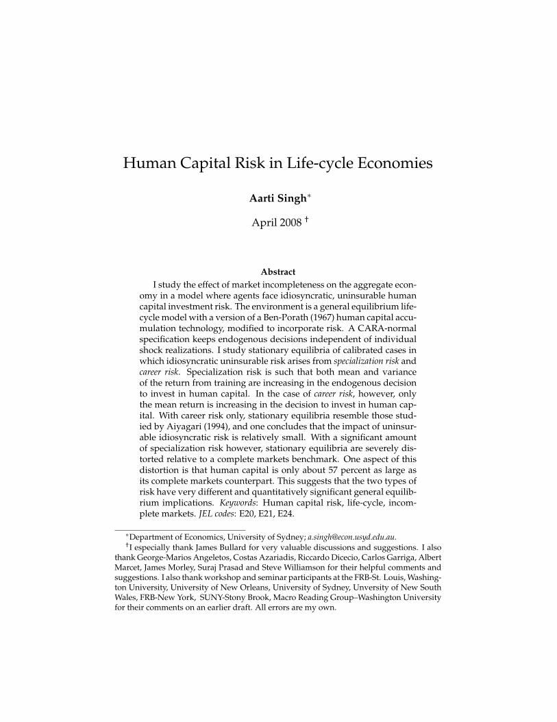
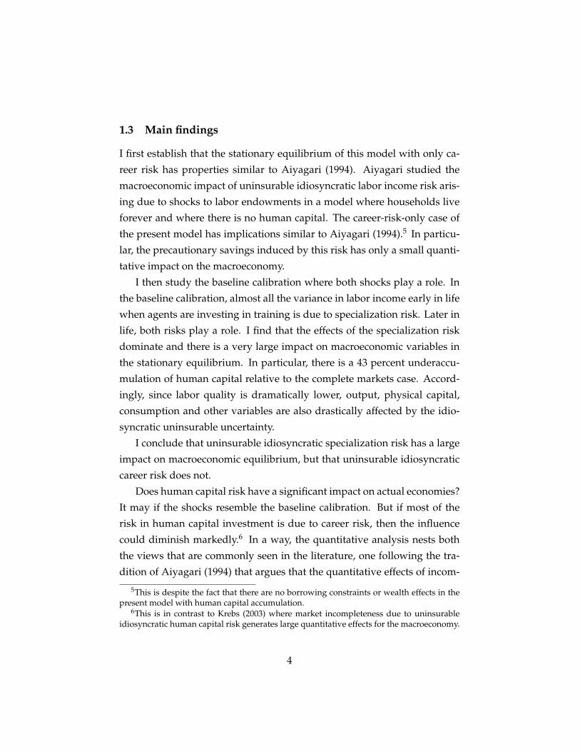
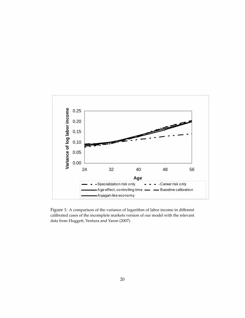
Figure 1: A comparison of the variance of logarithm of labor income in differentcalibrated cases of the incomplete markets version of our model with the relevantdata from Huggett, Ventura and Yaron (2007).

20

ibration economy. Table 1 reports the underlying standard deviation of the

sequence of shocks, fσε(t+ j)gj=5j=1 and fση(t+ j)gj=5

j=1, that are used in the

calibration of the incomplete markets version of these economies. As noted

earlier, the standard deviation of the two shocks varies across generations

but remains constant for agents within a generation at all times. Notice that

in this model there is no risk in the first period of life as agents have not yet

invested in training and in the last two periods after they retire. Figure 1

illustrates how this calibration strategy allows us to match the earnings dis-

persion generated by our model with Huggett, Ventura and Yaron’s (2007)

measure of the variance of labor earnings which is due to idiosyncratic hu-

man capital shocks. All the economies, except the specialization risk onlyeconomy, can be calibrated to match the data. Specialization risk interacts

with the time allocated to education, and agents invest in training only in

the first two periods of their life-cycle. Therefore in the specialization risk

only economy, the sequence of shocks cannot be calibrated to match the

increase in the variance of labor earnings over the life-cycle.28

4.2 Results

Following the calibration procedure described above, we study stationary

equilibria of calibrated economies to determine the quantitative macroeco-

nomic consequences of market incompleteness in a general equilibrium

life-cycle model.

standard deviation of the human capital shocks.27In our model, human capital investment refers to time the spent in education and hence

agents train for 6 years after the age of 16. Human capital risk is both multiplicative andadditive in our framework. In Huggett, Ventura and Yaron (2007) human capital shocksenter multiplicatively in the law of motion of human capital. For these shocks to play a roleover most of the life-cycle, they assume that agents invest time in training until they areclose to the retirement age. The time allocation problem, the trade-off between training andworking exists for most part of the life-cycle, an unrealistic implication of their model. Asa result, we consider that the risk identified in Huggett, Ventura and Yaron (2007) is in facta proxy for both the risks that the agents face over their life-cycle, specialization and careerrisk.

28The specification of risk in the specilization risk only economy is the following fσε(t+j)gj=5

j=1 = f1.732gj=5j=1 and fση(t+ j)gj=5

j=1 = f0gj=5j=1.

21

4.2.1 Aiyagari-like economy

We construct a version of Aiyagari (1994) in a life-cycle context, Aiyagari-like economy. Such a construction ensures that the predictions based on

an appropriately calibrated model, the Aiyagari-like economy, are consis-

tent with the quantitative findings of the existing literature that studies the

effect of uninsurable idiosyncratic labor income risk on the aggregate econ-

omy. In addition this construction rules out the likelihood that some of

the features of our model–life-cycle model with CARA preferences with no

wealth effects and no borrowing constraints–are shaping the main findings

of the paper.

Aiyagari (1994) studied uninsurable labor endowment risk in a model

with no human capital where agents live forever. This is a life-cycle model,

and unlike Aiyagari there are no borrowing constraints and no wealth ef-

fects. To collapse our model with human capital accumulation to an Aiyagari-

like economy, we set γ(t) and γ(t + 1) equal to zero such that agents do

not invest in training. Due to lack of education, specialization risk does

not play any role in this calibration. We endow the agents with an average

steady state labor quality x from our complete markets benchmark, column

1, panel B, Table 2. We set δh = 0. The rest of the parameters are calibrated

to meet the targets mentioned in the previous section.

Panel A of Table 2 reports the aggregate macroeconomic variables in the

stationary equilibrium of the Aiyagari-like economy. Both qualitative and

quantitative results in the Aiyagari-like economy are similar to Aiyagari

(1994). When markets are incomplete, the savings rate (which equals δkk/y)

increases relative to the complete markets benchmark but the increase is

not quantitatively significant. In Aiyagari (1994), the increase in the sav-

ings rate is in the range f0.06, 7.33g, expressed in percentage points.29 In

29In the quantitative analysis of Aiyagari (1994) logarithm of labor endowment shockfollows an AR(1) process with different values of the autoregressive coefficient and thecoefficient of variation based on various studies. He reports his results based on differentcombinations of relative risk aversion, coefficient of variation and serial correlation. SeeTable II in Aiyagari (1994). In reporting the range here, we do not consider the case wherethe net return on capital is negative, the last entry in Table II.

22

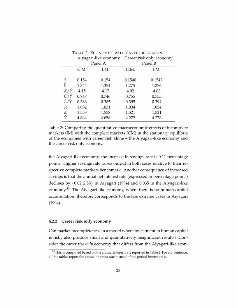
TABLE 2. ECONOMIES WITH CAREER RISK ALONE

Aiyagari-like economy Career risk only economyPanel A Panel B

C.M. I.M. C.M. I.M.

x 0.154 0.154 0.1540 0.1542k 1.344 1.354 1.275 1.276K/Y 4.15 4.17 4.02 4.03C/Y 0.747 0.746 0.755 0.755L/Y 0.386 0.385 0.395 0.394R 1.032 1.031 1.034 1.034w 1.553 1.558 1.521 1.521Y 4.644 4.658 4.272 4.276

Table 2: Comparing the quantitative macroeconomic effects of incompletemarkets (IM) with the complete markets (CM) in the stationary equilibriaof the economies with career risk alone – the Aiyagari-like economy andthe career risk only economy.

the Aiyagari-like economy, the increase in savings rate is 0.11 percentage

points. Higher savings rate raises output in both cases relative to their re-

spective complete markets benchmark. Another consequence of increased

savings is that the annual net interest rate (expressed in percentage points)

declines by f0.02, 2.88g in Aiyagari (1994) and 0.035 in the Aiyagari-like

economy.30 The Aiyagari-like economy, where there is no human capital

accumulation, therefore corresponds to the less extreme cases in Aiyagari

(1994).

4.2.2 Career risk only economy

Can market incompleteness in a model where investment in human capital

is risky also produce small and quantitatively insignificant results? Con-

sider the career risk only economy that differs from the Aiyagari-like econ-

30This is computed based on the annual interest rate reported in Table 2. For convenience,all the tables report the annual interest rate instead of the period interest rate.

23

omy along two dimensions, agents endogenously decide how much to

train and human capital depreciates to maintain a constant level of labor

quality in the stationary equilibrium.

Table 2, panel B presents results for the career risk only economy. Rel-

ative to the complete markets benchmark, incomplete markets have small

and quantitatively insignificant effects on the aggregate economy, even smaller

than the Aiyagari-like economy. Like the Aiyagari-like economy, the sav-

ings rate increases and output is also higher when markets are incomplete.

A striking result in the career risk only economy is that when markets are

incomplete there is overaccumulation of human capital, though quantita-

tively insignificant but in compliance with Angeletos and Calvet (2006).31

These results demonstrate that allowing agents to optimally decide how

much time to allocate to training when returns from training are uncertain

and uninsurable is not enough to generate large quantitative effects. More-

over, when individuals face career risk, the risk where a change in training

only affects the mean return but not the variance of the return from train-

ing, the effect of market incompleteness are marginal.

Our next specification of the incomplete markets incorporates special-

ization risk as well.

4.2.3 Baseline calibration economy

In the incomplete markets case of the baseline calibration economy, we as-

sume that agents face both risks. Since the empirical literature provides

no guidance on how to assign weights to these shocks, we assign these

weights in a way that attributes almost all the variability in labor earnings

to specialization risk early in the life-cycle and later, the additional risk that

agents face is entirely due to the career shocks. The reason behind such an

extreme calibration is that in this economy we want to explore the role of

specialization risk while still matching the data on life-cycle labor income

variability. From Figure 1 it is clear that specialization risk alone cannot

31Labor quality-output ratio also increases, albeit very marginally.

24

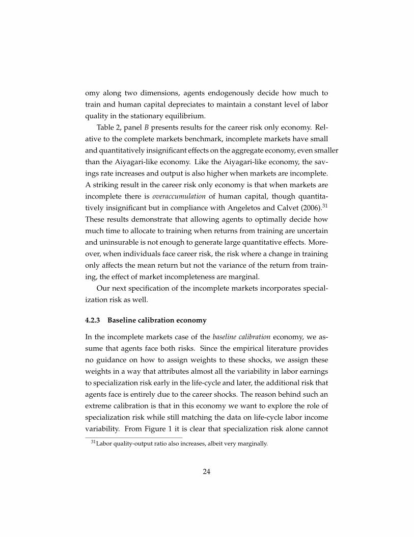
TABLE 3. BASELINE CALIBRATION

Complete markets Incomplete marketsx 0.154 0.088k 1.275 1.381K/Y 4.02 4.22C/Y 0.755 0.742L/Y 0.395 0.382R 1.034 1.030w 1.521 1.575Y 4.272 3.366

Table 3: Aggregate effects of market incompleteness in the stationary equi-librium of the baseline calibration economy.

match the data and hence we combine it with career risk.

As mentioned before, the two economies with endogenous training de-

cision, the career risk only economy and the baseline calibration economy,

differ only in the way the risks are calibrated. As a result, the complete

markets case is identical for the two economies, column 1 in panel B of Ta-

ble 2 and column 2 in Table 3. However, note that the stationary equilibria

with uninsurable idiosyncratic human capital risk are strikingly different.

The stationary equilibrium of the baseline calibration economy clearly il-

lustrates that the specialization risk plays a very crucial role in determining

the aggregate implications of market incompleteness. Market incomplete-

ness has a significant impact on human capital accumulation causing the

average labor quality to decline by 43 percent. This is in stark contrast with

the findings of Aiyagari (1994) where the quantitative effect of incomplete

markets was marginal. Agents self-insure in this economy by allocating

less time to training. Due to such a sharp decrease in average labor qual-

ity, capital and the labor supply reduce dramatically by 12 and 19 percent

respectively. Unlike the other economies studied here, output falls and the

decrease is substantial–17 percent relative to the complete markets bench-

mark. Like Aiyagari (1994) and other studies in this literature, agents in

this economy also insure themselves against the uninsurable risk by hold-

25

ing more risk-free assets. As a result, capital-output ratio increases by 4.9

percent, even though in the aggregate both capital and output fall relative

to the complete markets case. The annual net interest rate decreases by 0.37

percentage points.

In the baseline calibration economy, the underaccumulation of human

capital is large relative to the findings of Krebs (2003). In Krebs (2003) in-

vestment in human capital is 4.2 percentage points (of GDP) lower relative

to the complete markets case. The comparable number for this economy

is 19.8 percentage points.32 Therefore, not accounting for the time alloca-

tion problem in an economy where specialization risk is the main source

of uninsurable human capital risk can lead to a substantial misstatement

of the impact of risk on human capital investment. Investment in physical

capital in Krebs (2003) is 3.95 percentage points (of GDP) higher relative to

complete markets benchmark. In our baseline calibration economy, invest-

ment in physical capital relative to output, the savings rate, increases by

1.20 percentage points, an increase which is 1/3 of the increase in Krebs.

Therefore it appears that in this economy agents self insure but more by

altering their decision to train and less via the traditional precautionary

savings channel.

In the quantitative analysis we compared three different economies,

the Aiyagari-like economy, the career risk only economy and the baseline

calibration economy. Such a comparison is convincing in that all three

economies endogenously generate the same life-cycle pattern of labor in-

come variance even when they have extremely different aggregate macro-

economic implications. In the Aiyagari-like economy and the career risk

only economy, incomplete markets have very small quantitative effects.

On the contrary, the baseline calibration economy with higher weight on

specialization risk, market incompleteness decreases labor quality dramati-

32Investment in human capital in our model is captured by the time allocated to training.In the first period, time devoted to training relative to output (τ0/y) decreases by 19.2percentage points. The decrease is lower in the second period, 0.6 percentage points. Thusthe overall decrease in investment in human capital relative to output is 19.8 percentagepoints.

26

cally and all other aggregate variables are also impacted considerably. Thus

depending on the weights of the two shocks, the quantitative implications

of incomplete markets could be as large as our baseline case or as small as

the case with only career shocks. Unless empirical studies isolate the rel-

ative weights of these shocks in the data, it is hard to take a stand on the

exact role of market incompleteness.

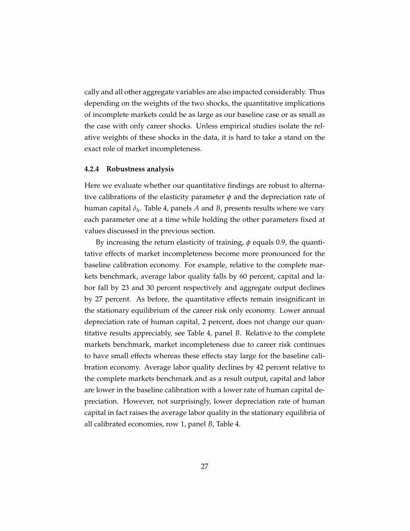
4.2.4 Robustness analysis

Here we evaluate whether our quantitative findings are robust to alterna-

tive calibrations of the elasticity parameter φ and the depreciation rate of

human capital δh. Table 4, panels A and B, presents results where we vary

each parameter one at a time while holding the other parameters fixed at

values discussed in the previous section.

By increasing the return elasticity of training, φ equals 0.9, the quanti-

tative effects of market incompleteness become more pronounced for the

baseline calibration economy. For example, relative to the complete mar-

kets benchmark, average labor quality falls by 60 percent, capital and la-

bor fall by 23 and 30 percent respectively and aggregate output declines

by 27 percent. As before, the quantitative effects remain insignificant in

the stationary equilibrium of the career risk only economy. Lower annual

depreciation rate of human capital, 2 percent, does not change our quan-

titative results appreciably, see Table 4, panel B. Relative to the complete

markets benchmark, market incompleteness due to career risk continues

to have small effects whereas these effects stay large for the baseline cali-

bration economy. Average labor quality declines by 42 percent relative to

the complete markets benchmark and as a result output, capital and labor

are lower in the baseline calibration with a lower rate of human capital de-

preciation. However, not surprisingly, lower depreciation rate of human

capital in fact raises the average labor quality in the stationary equilibria of

all calibrated economies, row 1, panel B, Table 4.

27

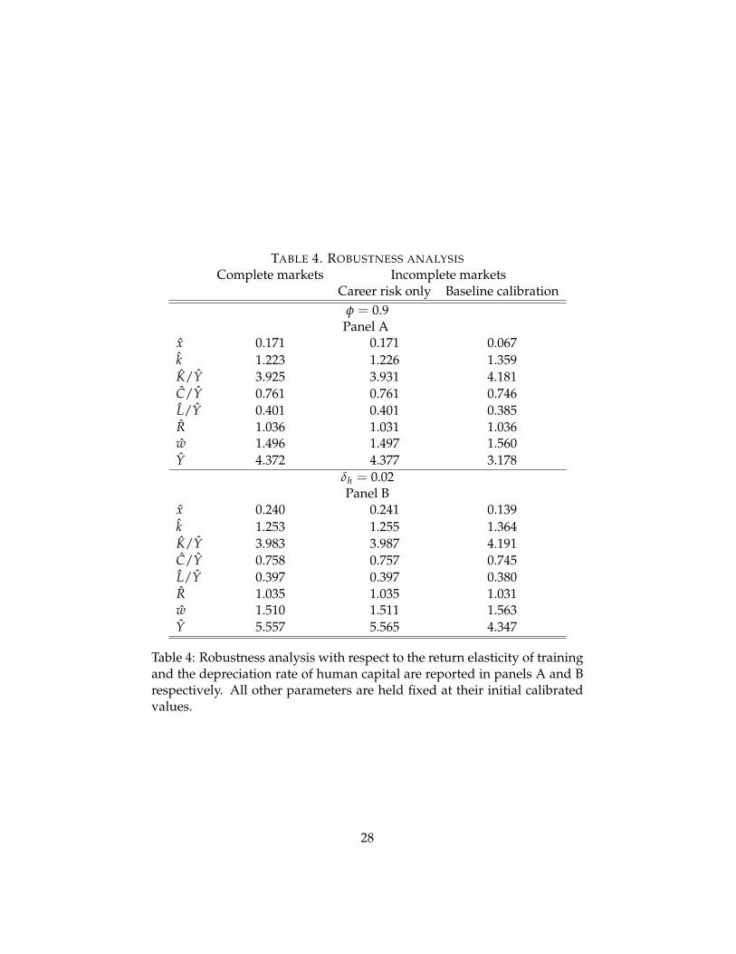
TABLE 4. ROBUSTNESS ANALYSIS

Complete markets Incomplete marketsCareer risk only Baseline calibration

φ = 0.9Panel A

x 0.171 0.171 0.067k 1.223 1.226 1.359K/Y 3.925 3.931 4.181C/Y 0.761 0.761 0.746L/Y 0.401 0.401 0.385R 1.036 1.031 1.036w 1.496 1.497 1.560Y 4.372 4.377 3.178

δh = 0.02Panel B

x 0.240 0.241 0.139k 1.253 1.255 1.364K/Y 3.983 3.987 4.191C/Y 0.758 0.757 0.745L/Y 0.397 0.397 0.380R 1.035 1.035 1.031w 1.510 1.511 1.563Y 5.557 5.565 4.347

Table 4: Robustness analysis with respect to the return elasticity of trainingand the depreciation rate of human capital are reported in panels A and Brespectively. All other parameters are held fixed at their initial calibratedvalues.

28

TABLE 5. TIME IN TRAINING

Complete markets Incomplete marketsCareer risk only Baseline calibration

Panel Aτ0 0.683 0.684 0.202τ1 0.066 0.067 0.054

Panel Bτ0 0.683 0.193τ1 0.066 0.049

Table 5: Fraction of one unit of time devoted to training in the first twoperiods of the life-cycle. No time is allocated to training thereafter. PanelsA and B report general equilibrium and partial equilibrium results respec-tively.

4.3 Life-cycle features of the model

In this section we take a closer look at the underlying training and asset

holding decisions in different calibrated economies with human capital ac-

cumulation – career risk only and baseline calibration economy. In these

economies, the training and asset holding decisions are identical for all the

agents within a generation. However, within generation heterogeneity due

to different realization of the shocks generates a distribution of earnings

and consumption for each cohort. As a result, we also explore the cross

sectional distribution of earnings and consumption implied by our model.

4.3.1 Individual decisions

Time allocated to training as a fraction of one unit of time in the first two

periods of the life-cycle, where each period corresponds to eight years, is

reported in Table 5. Panel A reports the overall effects whereas panel Bisolates the partial equilibrium effects of idiosyncratic uninsurable human

capital risk by holding wage and interest rate fixed at the complete markets

level.

In the case when there is no uncertainty, agents spend 6 years in train-

29

ing, 5.5 years between the age 16� 24 and half a year between 24� 32.33

When labor income uncertainty is due to career risk, the time allocated

to training does not change much relative to the complete markets bench-

mark, see column 3, panel A. However, in the baseline calibration where

specialization risk plays a central role, agents train for 2 years, 1.6 and 0.4

years in the first and second periods respectively. Relative to the complete

markets benchmark, training is merely 1/3 which is why labor quality is

dramatically lower in the stationary equilibrium of the baseline calibration

economy. As noted earlier this is a striking result.

Panel B evaluates the direct impact of risk on an individual’s training

decision when we hold wage and interest rate fixed at the complete mar-

kets level. From the two period case discussed in section 3 we know that

career risk does not directly influence the training decision. This is vali-

dated here in column 3, panel B as the level of training in the career risk

only economy is the same as in the complete markets benchmark, column

2, panel A. However, in the baseline calibration economy, time devoted to

training is even lower relative to the comparable case in panel A. Reducing

the time allocated to training lowers efficiency units but at the same time

it increases the time supplied to the labor market by an individual. Thus

the overall impact on the equilibrium wage rate is ambiguous in a general

equilibrium setting. However, we know that the wage rate increases in the

baseline calibration economy relative to the complete markets benchmark,

see Table 3. Not allowing the wage rate per efficiency unit to increase in

panel B partly explains why training is lower in this panel in relation to the

corresponding column in panel A.

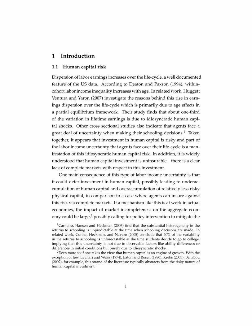
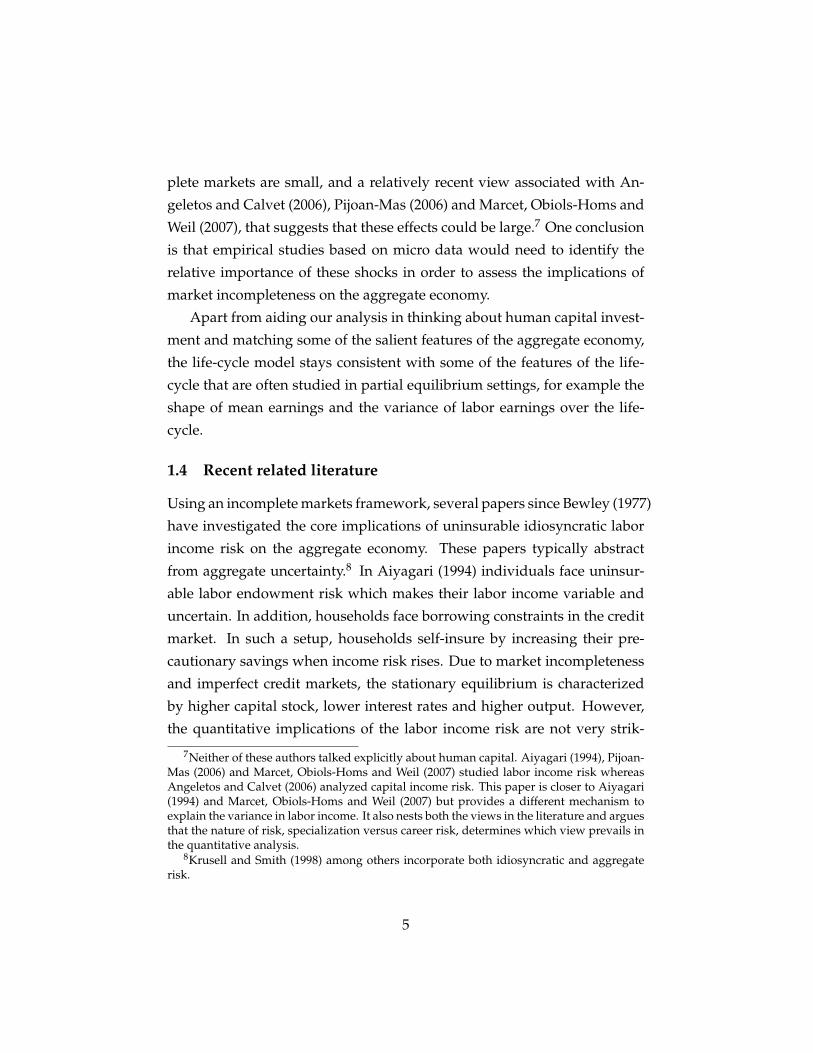
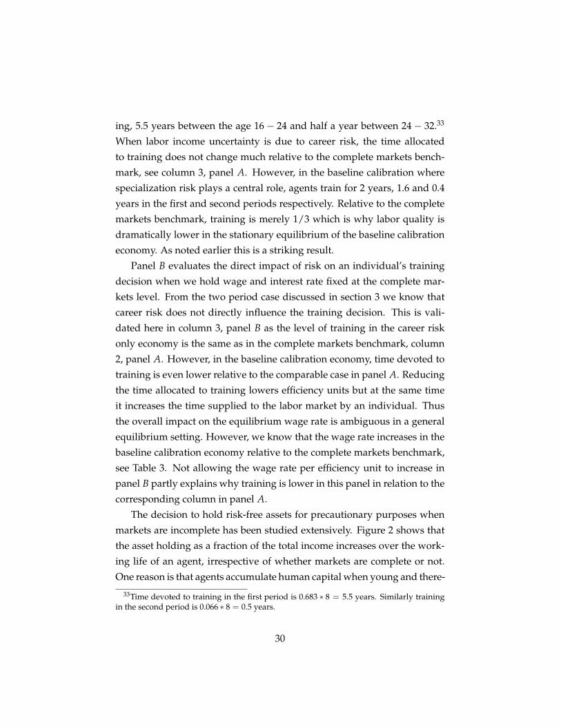
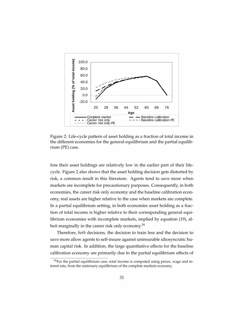
The decision to hold risk-free assets for precautionary purposes when

markets are incomplete has been studied extensively. Figure 2 shows that

the asset holding as a fraction of the total income increases over the work-

ing life of an agent, irrespective of whether markets are complete or not.

One reason is that agents accumulate human capital when young and there-

33Time devoted to training in the first period is 0.683 � 8 = 5.5 years. Similarly trainingin the second period is 0.066 � 8 = 0.5 years.

30

­20.0

0.0

20.0

40.0

60.0

80.0

100.0

20 28 36 44 52 60 68 76AgeA

sset

 hol

ding

 (% o

f tot

al in

com

e)

Complete market Baseline calibrationCareer risk only Baseline calibration­PECareer risk only­PE

Figure 2: Life-cycle pattern of asset holding as a fraction of total income inthe different economies for the general equilibrium and the partial equilib-rium (PE) case.

fore their asset holdings are relatively low in the earlier part of their life-

cycle. Figure 2 also shows that the asset holding decision gets distorted by

risk, a common result in this literature. Agents tend to save more when

markets are incomplete for precautionary purposes. Consequently, in both

economies, the career risk only economy and the baseline calibration econ-

omy, real assets are higher relative to the case when markets are complete.

In a partial equilibrium setting, in both economies asset holding as a frac-

tion of total income is higher relative to their corresponding general equi-

librium economies with incomplete markets, implied by equation (19), al-

beit marginally in the career risk only economy.34

Therefore, both decisions, the decision to train less and the decision to

save more allow agents to self-insure against uninsurable idiosyncratic hu-

man capital risk. In addition, the large quantitative effects for the baseline

calibration economy are primarily due to the partial equilibrium effects of

34For the partial equilibrium case, total income is computed using prices, wage and in-terest rate, from the stationary equilibrium of the complete markets economy.

31

020406080

100120140

20 28 36 44 52 60

Age

Mea

n la

bor i

ncom

e

Age effect, controlling time Baseline calibration

Career risk only

0.00

0.05

0.10

0.15

0.20

0.25

28 36 44 52 60

Age

Varia

nce 

of lo

g of

 labo

r inc

ome

Age effect, controlling time Baseline calibration

Career risk only

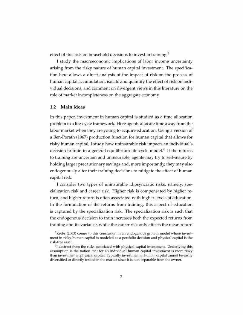
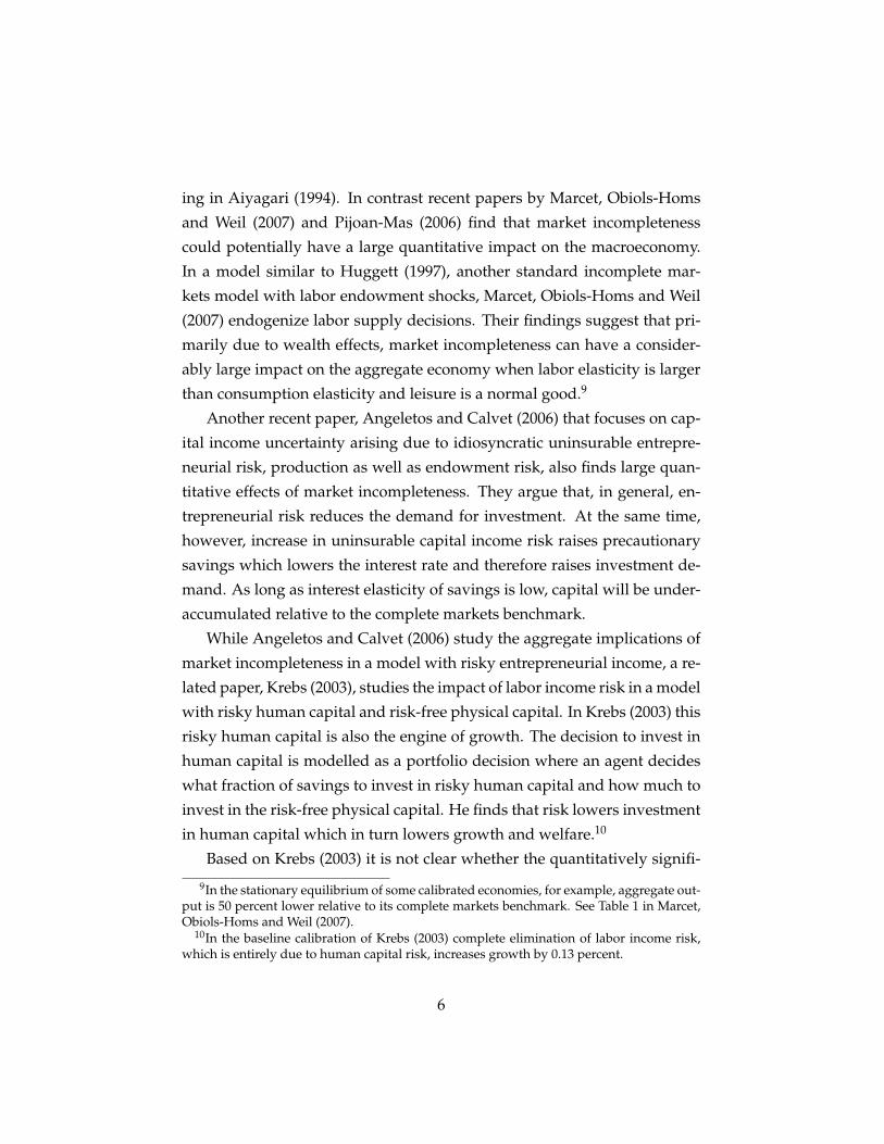
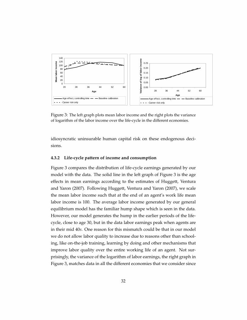
Figure 3: The left graph plots mean labor income and the right plots the varianceof logarithm of the labor income over the life-cycle in the different economies.

idiosyncratic uninsurable human capital risk on these endogenous deci-

sions.

4.3.2 Life-cycle pattern of income and consumption

Figure 3 compares the distribution of life-cycle earnings generated by our

model with the data. The solid line in the left graph of Figure 3 is the age

effects in mean earnings according to the estimates of Huggett, Ventura

and Yaron (2007). Following Huggett, Ventura and Yaron (2007), we scale

the mean labor income such that at the end of an agent’s work life mean

labor income is 100. The average labor income generated by our general

equilibrium model has the familiar hump shape which is seen in the data.

However, our model generates the hump in the earlier periods of the life-

cycle, close to age 30, but in the data labor earnings peak when agents are

in their mid 40s. One reason for this mismatch could be that in our model

we do not allow labor quality to increase due to reasons other than school-

ing, like on-the-job training, learning by doing and other mechanisms that

improve labor quality over the entire working life of an agent. Not sur-

prisingly, the variance of the logarithm of labor earnings, the right graph in

Figure 3, matches data in all the different economies that we consider since

32

­500

50100150200250300

20 28 36 44 52 60

Age

Mea

n co

nsum

ptio

n

Baseline calibration Career risk onlyBC plus 2stddev BC minus 2 stdevCR plus 2 stdev CR minus 2 stdev

+/­ 2 standard deviation bands

0.00

0.05

0.10

0.15

0.20

0.25

0.30

20 28 36 44 52 60

AgeVaria

nce 

of lo

g co

nsum

ptio

n

Baseline calibration Career risk only

Deaton Paxson

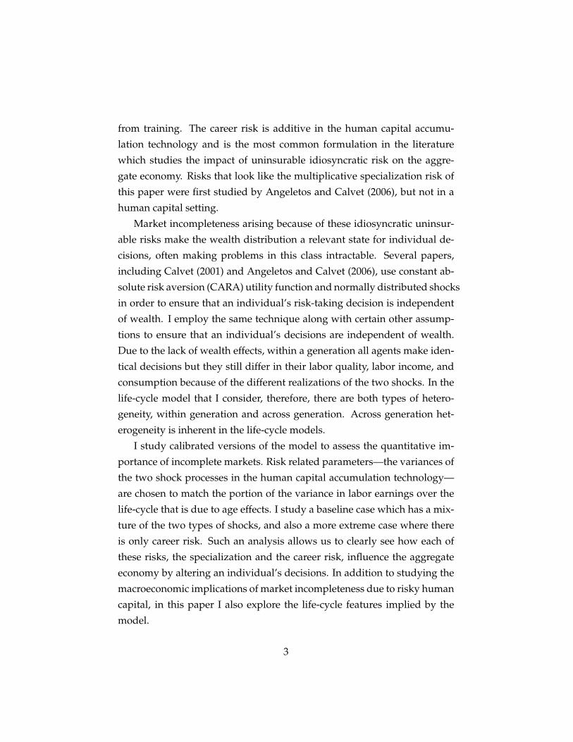
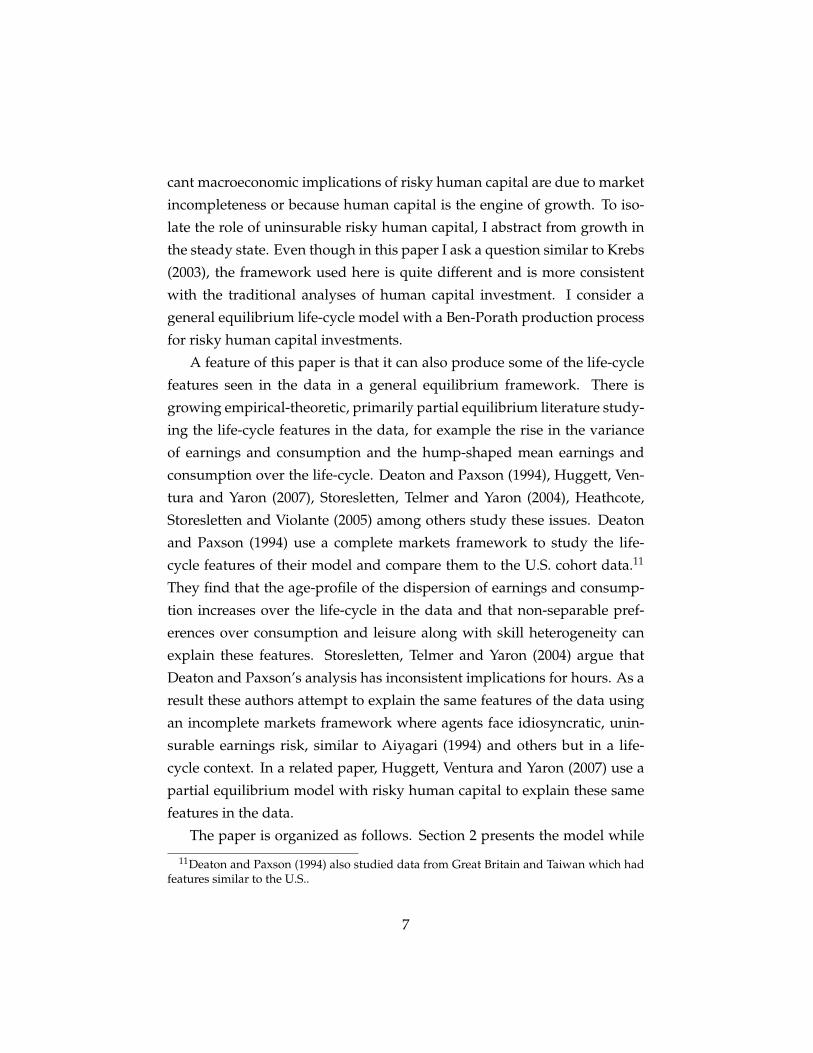
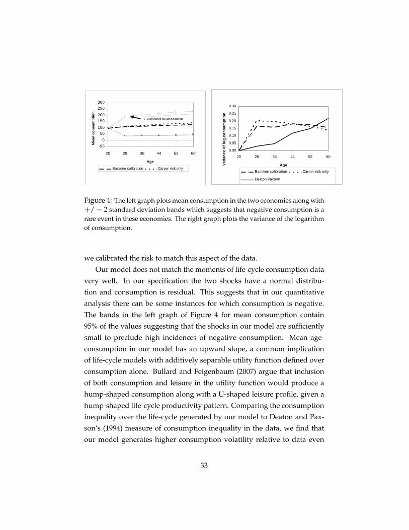
Figure 4: The left graph plots mean consumption in the two economies along with+/� 2 standard deviation bands which suggests that negative consumption is arare event in these economies. The right graph plots the variance of the logarithmof consumption.

we calibrated the risk to match this aspect of the data.

Our model does not match the moments of life-cycle consumption data

very well. In our specification the two shocks have a normal distribu-

tion and consumption is residual. This suggests that in our quantitative

analysis there can be some instances for which consumption is negative.

The bands in the left graph of Figure 4 for mean consumption contain

95% of the values suggesting that the shocks in our model are sufficiently

small to preclude high incidences of negative consumption. Mean age-

consumption in our model has an upward slope, a common implication

of life-cycle models with additively separable utility function defined over

consumption alone. Bullard and Feigenbaum (2007) argue that inclusion

of both consumption and leisure in the utility function would produce a

hump-shaped consumption along with a U-shaped leisure profile, given a

hump-shaped life-cycle productivity pattern. Comparing the consumption

inequality over the life-cycle generated by our model to Deaton and Pax-

son’s (1994) measure of consumption inequality in the data, we find that

our model generates higher consumption volatility relative to data even

33

when we account for just 1/3 of the variance in labor earnings.35 Storeslet-

ten, Telmer and Yaron (2004) suggest that without a social security system,

variance in consumption is roughly 20% higher relative to data. In this

model there is no form of social insurance and that could partly explain

high consumption variance. Another reason that our model generates high

consumption variance is that an agent’s endogenous decisions are unaf-

fected by the actual realization of the two shocks. This causes consumption

to be residual and therefore more volatile. Apart from being more volatile,

the variance of consumption generated by the model is concave whereas in

the data it is somewhat linear. In the model when agents are young, they

accumulate human capital which is risky and their holdings of risk-free as-

sets are relatively low. As a result shocks to training have a larger impact on

consumption in the early periods of the life-cycle. Over time as holdings of

risk-free asset increases, human capital shocks tend to have a lower impact.

Overall, in both the economies, the life-cycle consumption implications of

our model do not match data very well. By incorporating leisure, allowing

for wealth effects and introducing some form of social insurance, we could

potentially correct the implications of our model for consumption.

Even though the aggregate implications of these two economies with

incomplete markets, the career risk only economy and the baseline cali-

bration economy, are undoubtedly very different, the life-cycle features are

somewhat similar. The two economies endogenously generate the same

life-cycle pattern of labor income variability. Other life-cycle features, such

as mean labor income, mean consumption and the variance of consumption

over the life-cycle are also not very different across these two economies.

One reason could be that these divergent decisions occur only in the early

part of the life-cycle and their influence gets smoothed over many periods

thus understating the striking differences in the endogenous decisions in

the two economies with incomplete markets.

35Deaton and Paxson (1994) use consumption data from the Consumption ExpenditureSurvey (CEX), 1980-1990. They remove the cohort effects from the data when measuringthe age-profile of consumption inequality over the life-cycle. See Deaton and Paxson (1994)for further details.

34

5 Conclusion

This paper studies the impact of uninsurable idiosyncratic human capital

risk, using a Ben-Porath version of production function for human capital,

in a general equilibrium life-cycle model. Our results indicate that unin-

surable idiosyncratic human capital risk alone is not enough to generate

large quantitative macroeconomic effects, contrary to the earlier findings

in this literature. The nature of risk, career versus specialization, is crucial

in determining the quantitative implications of market incompleteness for

the aggregate economy. Calibrated stationary equilibrium with only career

risk has properties similar to Aiyagari (1994) reconfirming the long held be-

lief that the quantitative implications of uninsurable idiosyncratic risk are

inconsequential. However, our baseline calibration with high weight on

the specialization risk clearly illustrates that market incompleteness could

have large, quantitatively significant, macroeconomic implications. Sta-

tionary equilibrium in this case is severely distorted relative to the com-

plete markets benchmark.

Based on our quantitative analysis, we conclude that in order to com-

ment on the macroeconomic effect of uninsurable idiosyncratic human cap-

ital risk, empirical studies based on micro data would need to determine

the relative weights of these shocks in data. Even though the life-cycle fea-

tures generated by our model for different calibrations of risk are not very

different, the decision to train is particularly dissimilar in these economies.

This dissimilarity in the level of education is primarily due to specializa-

tion risk. Empirical cross country studies estimating risks associated with

different types of education that require varying degrees of specialization

could however be indicative of the level of specialization risk that exists

in these countries. Such studies could thereby alert us about the likely ex-

tent of distortion in these countries due to uninsurable idiosyncratic human

capital risk.

35

References

[1] Angeletos, G-M. 2006. “Uninsured Idiosyncratic Investment Risk and

Aggregate Saving.” Review of Economic Dynamics, forthcoming.

[2] Angeletos, G-M. and L.E. Calvet. 2006. “Idiosyncratic Production Risk,

Growth and the Business Cycle.” Journal of Monetary Economics, 53,

1095-1115.

[3] Aiyagari, S.R. 1994. “Uninsured Idiosyncratic Risk and Aggregate

Saving.” Quarterly Journal of Economics, 109, 659-684.

[4] Becker, G. 1993. “Human Capital: A Theoretical and Empirical Analy-

sis with Special Reference to Education.” Columbia UP: New York,

Third edition.

[5] Benabou, R. 2002. “Tax and Education Policy in a Heterogeneous

Agent Economy: What Levels of Redistribution Maximize Growth

and Efficiency?” Econometrica, 70, 481-517.

[6] Ben-Porath, Y. 1967. “The Production of Human Capital and the Life-

cycle of Earnings.” Journal of Political Economy, 75, 352–65.

[7] Bewley, T. 1977. “The Permanent Income Hypothesis: A Theoretical

Formulation.” Journal of Economic Theory, 16, 252-292.

[8] Browning, M., L. Hansen, and J. Heckman. 1999. “Micro Data and

General Equilibrium Models.” Handbook of Labor Economics, vol 3, El-

sevier, Amsterdam.

[9] Bullard, J. and J. Feigenbaum. 2007. “A Leisurely Reading of the Life-

cycle Consumption Data.” Journal of Monetary Economics, forthcoming.

[10] Caballero, R.J. 1990. “Consumption Puzzles and Precautionary Sav-

ings.” Journal of Monetary Economics, 25, 113-36.

[11] Calvet, L.E. 2001. “Incomplete Markets and Volatility.” Journal of Eco-nomic Theory, 98, 295-338.

36

[12] Card, D. 2001. “Estimating the Return to Schooling: Progress on Some

Econometric Problems.” Econometrica, 69, 1127-60.

[13] Carneiro, P., K.T. Hansen, and J. Heckman. 2003. “Estimating Distribu-

tions of Treatment Effects with an Application to Returns to Schooling

and Measurement of the Effects of Uncertainty on College.” Interna-tional Economic Review, 44, 361-422.

[14] Carroll, C. and M. Kimball. 2001. “Liquidity Constraints and Pre-

cautionary Saving.” NBER Working Paper Number 8496, http://www-

personal.umich.edu/~mkimball/pdf/liquid_nberwp.pdf

[15] Christiansen, C., J.S. Joensen, and H.S. Nielsen. 2006. “The Risk-

Return Trade-off in Human Capital Investment.” IZA, Discussion Pa-

per # 1962.

[16] Costain, J.S. and M. Reiter. 2005. “Stabilization versus Insurance: Wel-

fare Effects of Procyclical Taxation under Incomplete Markets.” man-

uscript.

[17] Cunha, F., J. Heckman, and S. Navaro. 2005. “Separating Uncertainty

from Heterogeneity in Life-cycle Earnings.” Oxford Economic Papers,

57, 191-261.

[18] Deaton, A. and C. Paxson. 1994. “Intertemporal Choice and Inequal-

ity.” Journal of Political Economy, 102, 437-67.

[19] Eaton, J. and H.S. Rosen. 1980. “Taxation, Human Capital and Uncer-

tainty.” American Economic Review, 70, 705-715.

[20] Hall, R.E. 2006. “Complete Markets as an Approximation to the Bew-

ley Equilibrium with Unemployment Risk.” manuscript.

[21] Heathcote, J., K. Storesletten, and G. Violante. 2005. “Two Views on

Inequality over the Life-cycle.” Journal of the European Economic Associ-ation: Papers and Proceedings, 765-75.

37

[22] Gomes, J., J. Greenwood, and S. Rebelo. 2001. “Equilibrium Unem-

ployment.” Journal of Monetary Economics, 48, 109-52.

[23] Griliches, Z. 1977. “Estimating the Returns to Schooling: Some Econo-

metric Problems.” Econometrica, 45, 1-22.

[24] Grossmann, V. 2006. “Risky Human Capital Investment, Income Dis-

tribution, and Macroeconomic Dynamics.” Journal of Macroeconomics,

forthcoming.

[25] Guvenen, F. 2007. “Learning Your Earning: Are Labour Income Shocks

Really Very Persistent?” American Economic Review, 97, 687-712.

[26] Hartog, J., H. van Ophem, and S.M. Bajdechi. 2004. “How Risky is

Investment in Human Capital?” CESifo Working paper No. 1261.

[27] Huggett, M. 1997. “The One-sector Growth Model with Idiosyncratic

Shocks: Steady States and Dynamics.” Journal of Monetary Economics,

39, 385-403.

[28] Huggett, M., G. Ventura, and A. Yaron. 2007. “Sources of Lifetime In-

equality.” manuscript.

[29] Krebs, T. 2003. “Human Capital Risk and Economic Growth.” Quar-terly Journal of Economics, 118, 709-744.

[30] Krusell, P. and A. Smith. 1998. “Income and Wealth Heterogeneity in

the Macroeconomy.” Journal of Political Economy, 106, 867–96.

[31] Levhari, D. and Y. Weiss. 1974. “The Effect of Risk on the Investment

of Human Capital.” American Economic Review, 70, 705-715.

[32] Magill, M. and M. Quinzii. 1996. “Theory of Incomplete Markets.”

Cambridge, MA: MIT Press.

[33] Manuelli, R. and A. Sheshadari. 2006. “Human Capital and the Wealth

of Nations.” University of Wisconsin, manuscript.

38

[34] Marcet, A., F. Obiols-Homs, and P. Weil. 2007. “Incomplete Markets,

Labor Supply and Capital Accumulation.” Journal of Monetary Eco-nomics, 54, 2621-2635.

[35] Palacios-Huerta, I. 2003. “An Empirical Analysis of the Risk Properties

of Human Capital Returns.” American Economic Review, 93, 948-964.

[36] Pereira, P.T. and P.S. Martins. 2002. “Is there a Risk-Return Link in

Education.” Economic Letters, 75, 1, 31-37.

[37] Pijoan-Mas, J. 2006. “Precautionary Savings or Working Longer

Hours?” Review of Economic Dynamics, 9, 326-352.

[38] Rios-Rull, J-V. 1996. “Life-cycle Economies and Aggregate Fluctua-

tions.” Review of Economic Studies, 63, 465-89.

[39] Rudanko, L. 2007. “Idiosyncratic and Aggregate Risk in a Frictional

Labor Market.” University of Chicago, manuscript.

[40] Skinner, J. 1988. “Risky Income, Life-cycle Consumption, and Precau-

tionary Savings.” Journal of Monetary Economics, 22, 237–55.

[41] Storesletten, K., C. Telmer, and A. Yaron. 2004. “Consumption and

Risk Sharing Over the Life-cycle.” Journal of Monetary Economics, 51,

609–33.

[42] Zeldes, S.P. 1989. “Optimal Consumption with Stochastic Income: De-

viations from Certainty Equivalence.” Quarterly Journal of Economics,104, 275–98.

39