Embed Size (px)
Citation preview
Clemson University Clemson University
TigerPrints TigerPrints
All Dissertations Dissertations
May 2021
Essays on Response to Entry Threats Essays on Response to Entry Threats
Jaejeong Shin Clemson University, [email protected]
Follow this and additional works at: https://tigerprints.clemson.edu/all_dissertations
Recommended Citation Recommended Citation Shin, Jaejeong, "Essays on Response to Entry Threats" (2021). All Dissertations. 2786. https://tigerprints.clemson.edu/all_dissertations/2786
This Dissertation is brought to you for free and open access by the Dissertations at TigerPrints. It has been accepted for inclusion in All Dissertations by an authorized administrator of TigerPrints. For more information, please contact [email protected].
Essays on Response to Entry Threats
A Dissertation
Presented to
the Graduate School of
Clemson University
In Partial Fulfillment
of the Requirements for the Degree
Doctor of Philosophy
Economics
by
Jaejeong Shin
May 2021
Accepted by:
Dr. Matthew S. Lewis, Committee Chair
Dr. F. Andrew Hanssen
Dr. Patrick L. Warren
Dr. Babur De los Santos
Abstract
My dissertation examines price responses to entry threats in oligopoly markets.
In the first chapter, I theoretically demonstrate that two possible motivations can cause
incumbent oligopolists to lower prices in response to a potential entrant’s appearance:
one is strategic entry deterrence, and the other is a breakdown in tacit collusion.
Previous studies have analyzed pre-entry price cutting as an entry-deterrence strategy
because, under incomplete information, it may signal to the potential competitor
that entry would be unprofitable. When it comes to oligopoly markets, a breakdown
in tacit collusion can also lead to such a price response. Oligopoly firms have the
possibility to tacitly coordinate prices higher than their competitive level. However,
as the threat of future entry decreases the relative payoff of coordination, they may
reduce the price level maintained in collusion.
Even though pre-entry price cutting is the common reaction of both motivations
in oligopoly, those two can be differentiated in terms of reduction patterns across the
likelihood of entry. In the first chapter, I construct an infinitely repeated game in which
two incumbent firms choose prices with the possibility of tacit collusion, expecting an
entrant appears to make one-shot entry decision. When strategic entry deterrence
is impossible so that pre-entry price cutting is only driven by a breakdown in tacit
collusion, the model suggests the magnitude of the pre-entry price cuts monotonically
increases as entry is more likely. On the other hand, the size of the pre-entry price
ii
cuts to deter entry is non-monotonic across the likelihood of entry when strategic
entry deterrence is the underlying motivation.
Relying on the first chapter’s testable predictions, I empirically examine the
underlying motivation of pre-entry price cutting in the U.S. passenger airline mar-
kets. At the beginning of the second chapter, I estimate oligopolists’ pre-entry price
cuts when they encounter Southwest Airlines as a potential entrant. To test the
monotonicity of the price reductions, I employ a two-stage regression model. In
the first stage, a regularized logistic regression is used to predict Southwest’s entry
probabilities. In the second stage, I formulate price changes after the entry threat as a
function of the predicted probability of entry and test whether the coefficients related
to running gradients imply the size of pre-entry price cuts changes monotonically or
non-monotonically. In conclusion, responses to Southwest’s entry threat appear to
result from a breakdown in tacit collusion. Incumbent carriers are shown to cut pre-
entry prices further when Southwest’s entry is more likely, consistent with the testable
prediction of a breakdown in tacit collusion rather than strategic entry deterrence.
As an extension of the second chapter, the third chapter employs incumbent
carriers’ price distribution (particularly percentiles of ticket fares) to test the motiva-
tion of pre-entry responses. The basic idea is to compare how incumbents adjust their
higher fares (paid by business travelers) and their lower fares (paid by leisure travelers)
in response to a threat of entry. To this end, quantile regressions are used to show
fare distributions change after Southwest becomes a potential entrant. It turns out
that compared to the lower quantiles of fares, incumbents discount more on the higher
quantiles of fares when incumbents are threatened by Southwest’s potential entry.
Based on the second chapter’s motivation tests, I show that such price reductions
of incumbent monopolists and oligopolists exhibit more consistent patterns with an
attempt to deter entry and a breakdown in tacit collusion, respectively.
iii

Dedication
To my wife Boyoung and my son Leo for their unconditional love and support.
iv

Acknowledgments
I have deep gratitude for my adviser, Dr. Matthew S. Lewis. His stimulating
engagement and unwavering support have made this journey particularly rewarding
and enjoyable. It has been a pleasure to learn economic thinking and modeling under
your guidance. This experience will lay the groundwork for my future professional
success. Thank you sincerely for everything.
I would like to express sincere appreciation to my committee members, Dr. F.
Andrew Hanssen, Dr. Patrick L. Warren, and Dr. Babur De los Santos for their many
helpful comments and suggestions.
I am also grateful to seminar participants of the Industrial Organization
workshop at Clemson University. I really appreciate Aspen, Shannon, and Shirong for
reading my paper and sharing their thoughts.
v

Contents
Title Page . . . . . . . . . . . . . . . . . . . . . . . . . . . . . . . . . . . i
Abstract . . . . . . . . . . . . . . . . . . . . . . . . . . . . . . . . . . . . ii
Dedication . . . . . . . . . . . . . . . . . . . . . . . . . . . . . . . . . . . iv
Acknowledgments . . . . . . . . . . . . . . . . . . . . . . . . . . . . . . . v
List of Tables . . . . . . . . . . . . . . . . . . . . . . . . . . . . . . . . . viii
List of Figures . . . . . . . . . . . . . . . . . . . . . . . . . . . . . . . . . ix
1 Pre-entry Price Cutting by Collusive Incumbents with a SupergameApproach . . . . . . . . . . . . . . . . . . . . . . . . . . . . . . . . . . 11.1 Introduction . . . . . . . . . . . . . . . . . . . . . . . . . . . . . . . . . 11.2 No-entry-deterrence Model . . . . . . . . . . . . . . . . . . . . . . . 41.3 Strategic Entry-deterrence Model . . . . . . . . . . . . . . . . . . . . 71.4 Testable Predictions . . . . . . . . . . . . . . . . . . . . . . . . . . . 141.5 Conclusion and Discussion . . . . . . . . . . . . . . . . . . . . . . . . 15
2 Pre-entry Price Cutting by Collusive Incumbents with an Appli-cation to the Airline Industry . . . . . . . . . . . . . . . . . . . . . . 212.1 Introduction . . . . . . . . . . . . . . . . . . . . . . . . . . . . . . . . . 212.2 Data and Sample Selection . . . . . . . . . . . . . . . . . . . . . . . . 232.3 Pre-entry Price Cuts in the Oligopoly Markets . . . . . . . . . . . . . 262.4 Descriptive Evidence of Breakdowns in Tacit Collusion . . . . . . . . 272.5 Hypothesis Testing for Monotonicity . . . . . . . . . . . . . . . . . . 332.6 Conclusion . . . . . . . . . . . . . . . . . . . . . . . . . . . . . . . . . 34
3 The Effect of Entry Threat on Incumbent Price Distribution: Ev-idence from the Airline Industry . . . . . . . . . . . . . . . . . . . . 473.1 Introduction . . . . . . . . . . . . . . . . . . . . . . . . . . . . . . . . 473.2 Data and Sample Selection . . . . . . . . . . . . . . . . . . . . . . . . 503.3 Empirical Specifications . . . . . . . . . . . . . . . . . . . . . . . . . 53
vi
3.4 Motivation Tests of Pre-entry Drops in High Percentiles of Fares . . 553.5 Conclusion . . . . . . . . . . . . . . . . . . . . . . . . . . . . . . . . . 59
Appendices . . . . . . . . . . . . . . . . . . . . . . . . . . . . . . . . . . . 70A Existence and Uniqueness of the Sustainable Price Function . . . . . . 71B Incentive Compatibility Constraints in Separating Equilibrium . . . . 72C Existence of Non-trivial Limit Pricing . . . . . . . . . . . . . . . . . . 73D The Regularized Logistic Regression via the Elastic Net Penalty . . . 75
References . . . . . . . . . . . . . . . . . . . . . . . . . . . . . . . . . . . 81
vii
List of Tables
2.1 Summary Statistics of Market in the Full Sample and the Sub-samples 362.2 Incumbent Oligopolists’ Pricing in Response to Southwest’s Entry
Threat and Actual Entry . . . . . . . . . . . . . . . . . . . . . . . . . 372.3 Incumbent Duopolists’ Pricing in Response to Southwest’s Entry Threat
and Actual Entry . . . . . . . . . . . . . . . . . . . . . . . . . . . . . 382.4 Motivation Tests for Markets Where Entry Is Preannounced . . . . . 392.5 Monotonicity Tests for Pre-entry Price Cuts in the Oligopoly and
Duopoly Incumbent Samples with the Parametric Specifications . . . 402.6 Monotonicity Tests for Pre-entry Price Cuts of the Incumbent Samples
with the Non-parametric Specification . . . . . . . . . . . . . . . . . . . 41
3.1 Price Distribution Changes of Incumbent Monopolists in Response toSouthwest’s Entry Threat and Actual Entry . . . . . . . . . . . . . . . 61
3.2 Price Distribution Changes of Incumbent Oligopolists in Response toSouthwest’s Entry Threat and Actual Entry . . . . . . . . . . . . . . 62
3.3 Price Distribution Changes of Incumbent Duopolists in Response toSouthwest’s Entry Threat and Actual Entry . . . . . . . . . . . . . . 63
3.4 Monotonicity Tests for Price Distribution Changes in Dominant andOligopoly Incumbent Markets with the Parametric Specifications . . 64
3.5 Monotonicity Tests for Pre-entry Drops in the Percentiles of Fares withthe Incumbent Samples and the Non-parametric Specification . . . . 65
D.1 A Confusion Matrix of the Probit and Regularized Logistic Regressions 80
viii
List of Figures
1.1 Timelines of No-entry-deterrence and Strategic Entry-deterrence Cases 171.2 The Monotonicity of the Size of Pre-entry Price Cuts Caused by Break-
downs in Tacit Collusion . . . . . . . . . . . . . . . . . . . . . . . . . 181.3 Pricing Schemes of h-type and l-type Incumbents in the Pre-entry Stage 191.4 The Non-monotonicity of the Size of Pre-entry Price Cuts Caused by
Attempts to Deter Entry . . . . . . . . . . . . . . . . . . . . . . . . . 20
2.1 Cross-sectional Distributions of the Estimated Probability of Entry . 422.2 The Parametrically Estimated Relationship between the Predicted Prob-
ability of Entry and the Size of Pre-entry Price Cuts in the Oligopolyand Duopoly Incumbent Markets . . . . . . . . . . . . . . . . . . . . 43
2.3 The Non-parametrically Estimated Relationship between the Percentilesof Predicted Entry Probabilities and the Size of Pre-entry Price Cutsin the Oligopoly and Duopoly Incumbent Markets . . . . . . . . . . . 44
2.4 The Non-parametrically Estimated Relationship between the Percentilesof Predicted Entry Probabilities and the Size of Pre-entry Price Cutsin the Dominant Incumbent Markets . . . . . . . . . . . . . . . . . . 45
2.5 The Histogram and Q-Q plot of Ellison and Ellison’s Test StatisticsUsing Bootstrap Sampling . . . . . . . . . . . . . . . . . . . . . . . . 46
3.1 The Linear Relationship between the Predicted Probability of Entryand the Price Distribution in the Oligopoly Incumbent Markets . . . 66
3.2 The Quadratic Relationship between the Predicted Probability of Entryand the Price Distribution in the Oligopoly Incumbent Markets . . . 67
3.3 The Non-parametrically Estimated Relationship between the Percentilesof Predicted Entry Probabilities and the Price distribution in theDominant Incumbent Markets . . . . . . . . . . . . . . . . . . . . . . 68
3.4 The Non-parametrically Estimated Relationship between the Percentilesof Predicted Entry Probabilities and the Price distribution in theOligopoly Incumbent Markets . . . . . . . . . . . . . . . . . . . . . . 69
ix

Chapter 1
Pre-entry Price Cutting by
Collusive Incumbents with a
Supergame Approach
1.1 Introduction
A growing body of empirical evidence has demonstrated that incumbent firms’
behavior can be substantially influenced by the presence of a potential entrant, even
before entry occurs. More importantly, many empirical studies reveal price responses
to the threat of future entry (Goolsbee and Syverson, 2008; Seamans, 2013; Sweeting
et al., 2020). For example, incumbent carriers cut ticket fares when Southwest Airlines
becomes a potential entrant in a market, as found by Goolsbee and Syverson (2008).
Such price responses are often characterized as attempts by incumbents to deter
potential rivals from entering their market. Since Bain’s (1949) analysis, theoretical
studies have shown the incumbent price responses are profitable as an attempt to
deter entry. Milgrom and Roberts (1982a) demonstrate that limit pricing, setting a
1

pre-entry price below the monopoly price to deter entry, achieves its goal by convincing
a potential rival that entry is unprofitable.
Earlier studies on limit pricing have generally focused on incumbent monopolists
responding to potential entrants with a desire to deter entry. In oligopoly markets,
however, incumbent firms may have an alternative motivation for lowering prices in
the presence of a potential entrant. If incumbent oligopolists are tacitly colluding, a
threat of future entry increases the relative payoff of cheating, making it more difficult
to maintain higher price levels even prior to actual entry.1
To more-clearly motivate empirical examination in the next chapter, this study
theoretically demonstrates that these two explanations, a breakdown in tacit collusion
and an attempt to deter entry, provide different testable predictions concerning incum-
bent oligopolists’ pre-entry price cuts. The difference between those two predictions
is related to price cutting patterns. If incumbents cut prices to deter entry, the most
significant drop must be observed when the likelihood of entry is intermediate because
entry deterrence is most effective unless the entry is almost certain or extremely
unlikely. On the other hand, collusion is more likely to break down as the likelihood
of entry increases. Therefore, a breakdown in tacit collusion leads to the biggest drop
when entry is inevitable.
This study theoretically deals with two oligopoly pricing cases: one with no
entry-deterrence incentive and one with a strategic entry-deterrence incentive. As
a baseline, the model with no entry-deterrence incentive uses an infinitely repeated
game and assumes complete information. Under complete information, limit pricing
has no impact on an entrant’s decision making. Thus, a breakdown in tacit collusion
is the only source of pre-entry price cuts. Alternatively, the model with a strategic
1Using a finite horizon game, existing studies have theoretically examined oligopoly limit pricing(Harrington Jr, 1987; Bagwell and Ramey, 1991; Martin, 1995). However, they have not consideredthat the possibility of tacit collusion can also result in pre-entry price cuts.
2

entry-deterrence incentive assumes the potential entrant has incomplete information
about the incumbents’ costs. This assumption allows the model to incorporate the
possibility that incumbents cut their pre-entry prices to signal to the potential entrant
that they are strong (low cost) competitors and discourage entry even when it would
have been profitable.
The theoretical study is the first attempt to directly consider both the impact
of potential entry on tacit collusion and the possibility of limit pricing by tacitly
colluding incumbent oligopolists. A novel finding is that the reduction patterns of
pre-entry prices differ between a breakdown in tacit collusion and an attempt to deter
entry. In the no-entry-deterrence case, the size of pre-entry price reductions becomes
larger when entry is more likely to occur because the expectation of future entry makes
it more difficult to tacitly coordinate higher prices in the pre-entry stage. However,
in the strategic entry-deterrence case, limit pricing is most profitable when entry is
reasonably likely but not certain, while it is of little use when entry is either highly
unlikely or almost certain. These properties will cause the magnitude of pre-entry
price reductions to be non-monotonic in the likelihood of entry.
The paper continues as follows. Section 1.2 analyzes an infinite horizon game
under complete information regarding the effect of breakdowns in tacit collusion on
pre-entry pricing without a strategic entry-deterrence incentive. Section 1.3 applies
this game to incomplete information to incorporate the possibility of strategic entry
deterrence. Section 1.4 elaborates on the testable predictions derived from those two
cases. Section 1.5 concludes.
3
1.2 No-entry-deterrence Model
I construct a theoretical model of oligopoly competitors facing potential entry.
Throughout Section 1.2 and 1.3, the model deals with the two incentives of pre-
entry price cutting, a breakdown in tacit collusion and an attempt to deter entry.
While the former case assumes complete information, the latter incorporates imperfect
information and the potential for entry deterrence through limit pricing behavior as
in Milgrom and Roberts (1982a).
In both cases, incumbent duopolists with identical marginal costs engage in
infinitely repeated price competition with the potential to tacitly coordinate prices, as
documented by Friedman (1971). When tacitly colluding firms encounter a potential
entrant, collusion becomes more difficult in the face of lower expected future profits.
Thus, collusion provides an additional potential reason why incumbents might lower
prices in response to an entry threat. Comparing the predictions across models with
and without the potential for entry deterrence highlights testable differences that will
motivate the empirical analysis in Section 2.4 and 2.5.
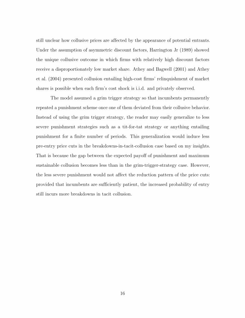
A timeline of the no-entry-deterrence case is summarized in the upper panel
of Figure 1.1. As mentioned earlier, the marginal costs of incumbents are commonly
known before the game starts. In the first stage, incumbent duopolists determine
their pre-entry prices, recognizing that a potential entrant will make entry decision
in the next stage. In the second stage, the potential entrant learns the incumbents’
prices and chooses whether to enter the market, comparing her future profit stream
with the entry cost K. In the third stage, firms compete as either duopoly or triopoly
(depending on the entry decision) and repeat the stage game afterward without any
further entry threats.
I assume that the entry cost K is stochastic in the first stage with CDF FK(k)
4
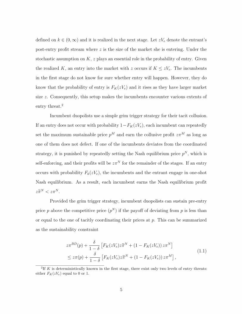
defined on k ∈ (0,∞) and it is realized in the next stage. Let zVe denote the entrant’s
post-entry profit stream where z is the size of the market she is entering. Under the
stochastic assumption on K, z plays an essential role in the probability of entry. Given
the realized K, an entry into the market with z occurs if K ≤ zVe. The incumbents
in the first stage do not know for sure whether entry will happen. However, they do
know that the probability of entry is FK(zVe) and it rises as they have larger market
size z. Consequently, this setup makes the incumbents encounter various extents of
entry threat.2
Incumbent duopolists use a simple grim trigger strategy for their tacit collusion.
If an entry does not occur with probability 1−FK(zVe), each incumbent can repeatedly
set the maximum sustainable price pM and earn the collusive profit zπM as long as
one of them does not defect. If one of the incumbents deviates from the coordinated
strategy, it is punished by repeatedly setting the Nash equilibrium price pN , which is
self-enforcing, and their profits will be zπN for the remainder of the stages. If an entry
occurs with probability Fk(zVe), the incumbents and the entrant engage in one-shot
Nash equilibrium. As a result, each incumbent earns the Nash equilibrium profit
zπN < zπN .
Provided the grim trigger strategy, incumbent duopolists can sustain pre-entry
price p above the competitive price (pN) if the payoff of deviating from p is less than
or equal to the one of tacitly coordinating their prices at p. This can be summarized
as the sustainability constraint
zπBD(p) +δ
1− δ[FK(zVe)zπ
N + (1− FK(zVe)) zπN]
≤ zπ(p) +δ
1− δ[FK(zVe)zπ
N + (1− FK(zVe)) zπM],
(1.1)
2If K is deterministically known in the first stage, there exist only two levels of entry threats:either FK(zVe) equal to 0 or 1.
5
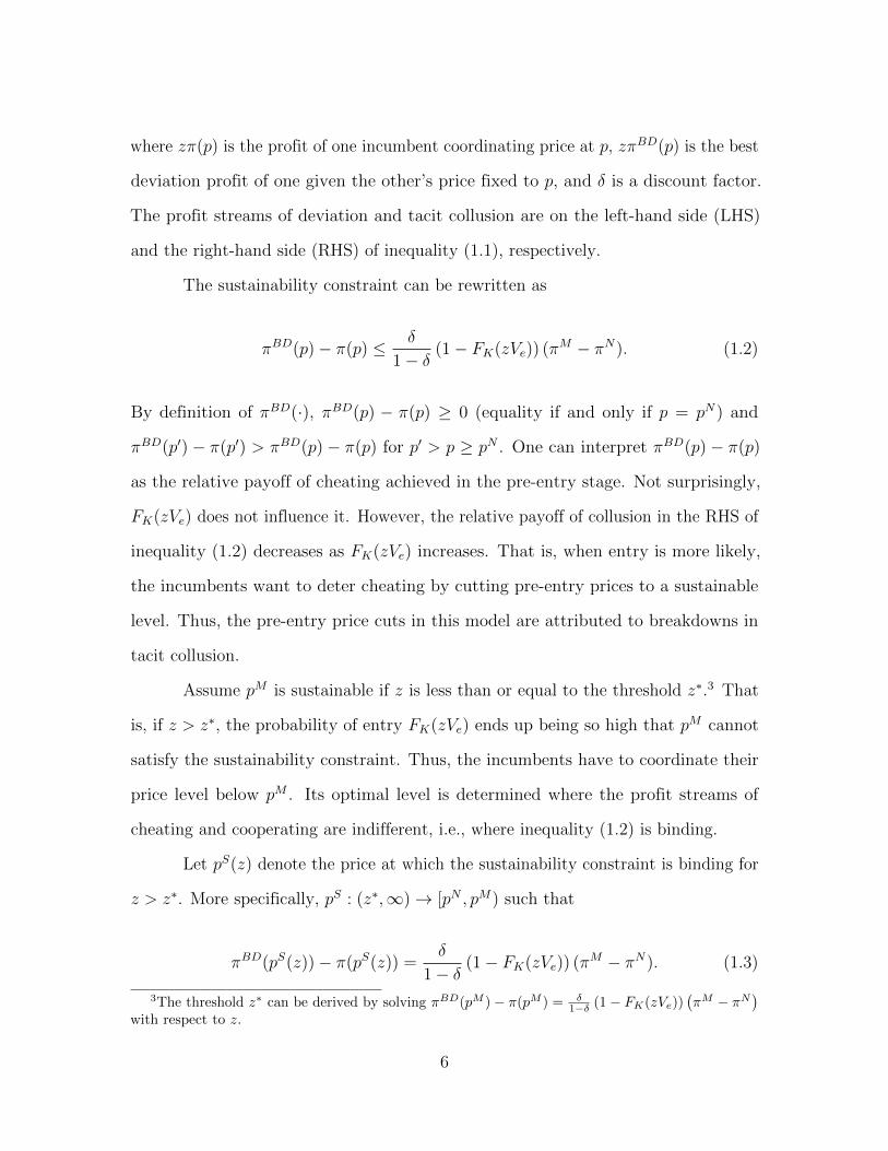
where zπ(p) is the profit of one incumbent coordinating price at p, zπBD(p) is the best
deviation profit of one given the other’s price fixed to p, and δ is a discount factor.
The profit streams of deviation and tacit collusion are on the left-hand side (LHS)
and the right-hand side (RHS) of inequality (1.1), respectively.
The sustainability constraint can be rewritten as
πBD(p)− π(p) ≤ δ
1− δ(1− FK(zVe)) (πM − πN). (1.2)
By definition of πBD(·), πBD(p) − π(p) ≥ 0 (equality if and only if p = pN) and
πBD(p′)− π(p′) > πBD(p)− π(p) for p′ > p ≥ pN . One can interpret πBD(p)− π(p)
as the relative payoff of cheating achieved in the pre-entry stage. Not surprisingly,
FK(zVe) does not influence it. However, the relative payoff of collusion in the RHS of
inequality (1.2) decreases as FK(zVe) increases. That is, when entry is more likely,
the incumbents want to deter cheating by cutting pre-entry prices to a sustainable
level. Thus, the pre-entry price cuts in this model are attributed to breakdowns in
tacit collusion.
Assume pM is sustainable if z is less than or equal to the threshold z∗.3 That
is, if z > z∗, the probability of entry FK(zVe) ends up being so high that pM cannot
satisfy the sustainability constraint. Thus, the incumbents have to coordinate their
price level below pM . Its optimal level is determined where the profit streams of
cheating and cooperating are indifferent, i.e., where inequality (1.2) is binding.
Let pS(z) denote the price at which the sustainability constraint is binding for
z > z∗. More specifically, pS : (z∗,∞)→ [pN , pM) such that
πBD(pS(z))− π(pS(z)) =δ
1− δ(1− FK(zVe)) (πM − πN). (1.3)
3The threshold z∗ can be derived by solving πBD(pM )− π(pM ) = δ1−δ (1− FK(zVe))
(πM − πN
)with respect to z.
6
Then, the equilibrium pricing of the no-entry-deterrence case can be summarized in
the following proposition.
Proposition 1.2.1. In the no-entry-deterrence case, incumbents can tacitly coor-
dinate pre-entry prices at the maximum sustainable level pM if the market size is
sufficiently small (z ≤ z∗). If the market size is sufficiently large (z > z∗), they
lower pre-entry prices along the sustainable price function pS(z) ∈ [pN , pM) due to a
breakdown in tacit collusion.
Notice that limz→+∞ pS(z) = pN . The proof of existence and uniqueness of pS(z) is
provided in Appendix A.
The reduction pattern triggered by a breakdown in tacit collusion can be
summarized as
Proposition 1.2.2. The sustainable price pS(z), which occurs below the maximum
sustainable level pM , is monotonic in the probability of entry FK(zVe).
It can be shown through the derivative of equation (1.3) as follows:
∂pS(z)
∂z=− δ
1−δVefK(zVe)(πM − πN)
∂πBD(p)∂p
∣∣∣p=pS(z)
− ∂π(p)∂p
∣∣∣p=pS(z)
< 0. (1.4)
The last inequality is true since ∂πBD(p)∂p
− ∂π(p)∂p≥ 0, ∀p ∈ [pN , pM ). Using a numerical
example, Figure 1.2 also demonstrates the monotonicity of pre-entry price cuts caused
by breakdowns in tacit collusion with respect to FK(zVe) and z.
1.3 Strategic Entry-deterrence Model
Next, I consider the strategic entry-deterrence case in which incumbent
duopolists can engage in limit pricing because of incomplete information on marginal
7
cost c. For simplicity, suppose there are two types of incumbents: h-type ones with
c = ch and l-type ones with c = cl such that ch > cl > 0. As shown in the lower
panel of Figure 1.1, the timeline of the strategic entry-deterrence case is similar to
the no-entry-deterrence case except that the cost type of incumbents is revealed to
the potential entrant after her entry decision. Hence, pre-entry prices can play a role
as signals regarding the entrant’s post-entry profitability since her post-entry profits
critically hinge on the incumbents’ cost type.
In the next subsections, I examine the existence of limit pricing as an entry-
deterrence strategy in a separating and pooling equilibrium. In a separating equilibrium,
l-type incumbents have an incentive to use limit pricing to be differentiated from
h-type. In contrast, h-type incumbents are encouraged to use limit pricing in a pooling
equilibrium since it helps them pretend to be l-type.
1.3.1 Separating Equilibrium
Belief System and Entry Decision of the Potential Entrant In a separating
equilibrium, the entrant updates her posterior belief on cost types µh : {ch, cl} → [0, 1].
Given the pre-entry prices (pi, pj) and market size z, the posterior belief on ch is
µh(ch|pi, pj, z) =
0 if pi, pj ≤ p(z);
1 otherwise,
(1.5)
where p(z) is an upper bound of pre-entry prices to convince the entrant that the
incumbents with market size z are l-type. Both pi and pj should be less than p(z) in
order to signal l-type.
After K is realized in the second stage, the entrant makes entry decision
8
following the pure strategy se : R+ × R+ → {Enter,NotEnter} defined as
se(pi, pj|µh, z) =
Enter if K < z E(Ve);
NotEnter otherwise,
(1.6)
where z E(Ve) is the entrant’s expected post-entry profit stream. Provided the posterior
belief µh, z E(Ve) = z[µh(ch|pi, pj, z)Ve,h + (1 − µh(ch|pi, pj, z))Ve,l], where Ve,τ for
τ ∈ {h, l} is the entrant’s post-entry profit stream (per unit of market size) against
τ -type incumbents.
Given the entrant’s belief and decision rule in a separating equilibrium, τ -type
incumbents encounter the probability of entry
FK(z E(Ve)) =
FK,l(z) if pi, pj ≤ p(z);
FK,h(z) otherwise,
(1.7)
where FK,τ (z) = FK(zVe,τ ) for τ ∈ {h, l}. The probability of entry in a separating
equilibrium is a function of pre-entry prices, not of the incumbents’ true type. It
means that if h-type incumbents mimic the l-type’s signal, the entry probability they
encounter will be FK,l(z), which is less than FK,h(z).
Strategy Profile of the Incumbents I claim that l-type incumbents can cut
pre-entry prices to the extent that h-type incumbents cannot mimic. Let p∗τ (z) denote
the τ -type’s equilibrium pricing of the no-entry-deterrence case, i.e.,
p∗τ (z) =
pMτ if z ≤ z∗;
pSτ (z) if z > z∗.
(1.8)
9
Since h-type incumbents cannot declare the l-type’s signal to deter entry, they end
up adhering to p∗h(z) as their next best strategy.
Given that h-type incumbents choose p∗h(z), l-type incumbents set limit price
pl based on the following two constraints: the incentive compatibility constraints of
h-type (ICh) and l-type (ICl). These constraints are represented as
(ICh) : πh(pl) ≤ πh(p∗h(z))− δ
1− δ(FK,h(z)− FK,l(z)) (πMh − πNh ), (1.9)
and
(ICl) : πl(pl) ≥ πl(p∗l (z))− δ
1− δ(FK,h(z)− FK,l(z)) (πMl − πNl ), (1.10)
where those with the subscript τ denote the corresponding variables of τ -type incum-
bents.4
The optimal limit price pLPl (z) is determined by ICh and ICl. Given market
size thresholds z2 > z1 > 0,
pLPl (z) =
pl(z) ≤ p∗l (z) if z ∈ [z1, z2];
p∗l (z) otherwise,
(1.11)
where pl(z) is the l-type’s non-trivial limit pricing that makes ICh binding, i.e.,
πh(pl(z)) = πh(p∗h(z))− δ
1− δ(FK,h(z)− FK,l(z))(πMh − πNh ). (1.12)
Note that the sustainability constraint still influences the l-type’s limit pricing in this
model.
4Appendix B provides more details about ICh and ICl.
10
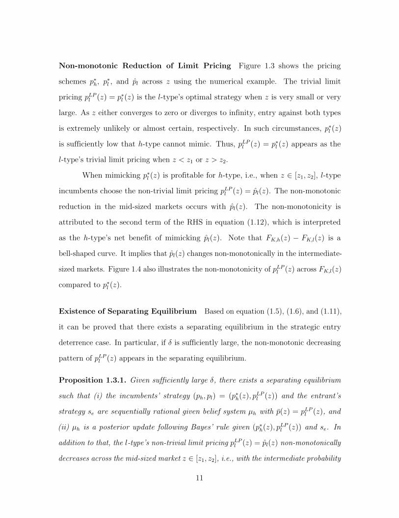
Non-monotonic Reduction of Limit Pricing Figure 1.3 shows the pricing
schemes p∗h, p∗l , and pl across z using the numerical example. The trivial limit
pricing pLPl (z) = p∗l (z) is the l-type’s optimal strategy when z is very small or very
large. As z either converges to zero or diverges to infinity, entry against both types
is extremely unlikely or almost certain, respectively. In such circumstances, p∗l (z)
is sufficiently low that h-type cannot mimic. Thus, pLPl (z) = p∗l (z) appears as the
l-type’s trivial limit pricing when z < z1 or z > z2.
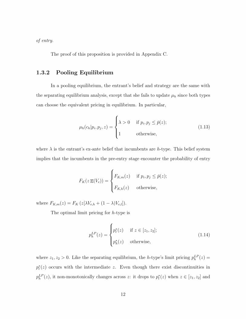
When mimicking p∗l (z) is profitable for h-type, i.e., when z ∈ [z1, z2], l-type
incumbents choose the non-trivial limit pricing pLPl (z) = pl(z). The non-monotonic
reduction in the mid-sized markets occurs with pl(z). The non-monotonicity is
attributed to the second term of the RHS in equation (1.12), which is interpreted
as the h-type’s net benefit of mimicking pl(z). Note that FK,h(z) − FK,l(z) is a
bell-shaped curve. It implies that pl(z) changes non-monotonically in the intermediate-
sized markets. Figure 1.4 also illustrates the non-monotonicity of pLPl (z) across FK,l(z)
compared to p∗l (z).
Existence of Separating Equilibrium Based on equation (1.5), (1.6), and (1.11),
it can be proved that there exists a separating equilibrium in the strategic entry
deterrence case. In particular, if δ is sufficiently large, the non-monotonic decreasing
pattern of pLPl (z) appears in the separating equilibrium.
Proposition 1.3.1. Given sufficiently large δ, there exists a separating equilibrium
such that (i) the incumbents’ strategy (ph, pl) = (p∗h(z), pLPl (z)) and the entrant’s
strategy se are sequentially rational given belief system µh with p(z) = pLPl (z), and
(ii) µh is a posterior update following Bayes’ rule given (p∗h(z), pLPl (z)) and se. In
addition to that, the l-type’s non-trivial limit pricing pLPl (z) = pl(z) non-monotonically
decreases across the mid-sized market z ∈ [z1, z2], i.e., with the intermediate probability
11
of entry.
The proof of this proposition is provided in Appendix C.
1.3.2 Pooling Equilibrium
In a pooling equilibrium, the entrant’s belief and strategy are the same with
the separating equilibrium analysis, except that she fails to update µh since both types
can choose the equivalent pricing in equilibrium. In particular,
µh(ch|pi, pj, z) =
λ > 0 if pi, pj ≤ p(z);
1 otherwise,
(1.13)
where λ is the entrant’s ex-ante belief that incumbents are h-type. This belief system
implies that the incumbents in the pre-entry stage encounter the probability of entry
FK(z E(Ve)) =
FK,m(z) if pi, pj ≤ p(z);
FK,h(z) otherwise,
where FK,m(z) = FK (z[λVe,h + (1− λ)Ve,l]).
The optimal limit pricing for h-type is
pLPh (z) =
p∗l (z) if z ∈ [z1, z2];
p∗h(z) otherwise,
(1.14)
where z1, z2 > 0. Like the separating equilibrium, the h-type’s limit pricing pLPh (z) =
p∗l (z) occurs with the intermediate z. Even though there exist discontinuities in
pLPh (z), it non-monotonically changes across z: it drops to p∗l (z) when z ∈ [z1, z2] and
12

then jump up to p∗h(z) when z > z2.
Note that the h-type’s limit pricing p∗l (z) is profitable in the same intermediate-
sized market with the separating equilibrium analysis. It is based on ICh: when
z ∈ [z1, z2], mimicking p∗l (z) ends up better for h-type than adhering to p∗h(z) in
a pooling equilibrium as well. As opposed to the separating equilibrium, l-type
incumbents in a pooling equilibrium have no incentive to cut price below p∗l (z) to be
differentiated from h-type because the entrant cannot update her posterior belief even
if prices lower than p∗l (z) are observed.
Based on equation (1.6), (1.13), and (1.14), the existence of a pooling equilib-
rium can be shown.
Proposition 1.3.2. Given sufficiently large δ, there exists a pooling equilibrium such
that (i) the incumbents’ strategy (ph, pl) = (pLPh (z), p∗l (z)) and the entrant’s strategy
se are sequentially rational given belief system µh with p(z) = p∗l (z), and (ii) µh is
a posterior update following Bayes’ rule given (pLPh (z), p∗l (z)) and se. In addition to
that, the h-type’s limit pricing pLPh (z) non-monotonically decreases across z since
they drop prices below p∗h(z) in order to mimic p∗l (z) when z ∈ [z1, z2], i.e., with the
intermediate probability of entry.
The proof of this proposition is omitted in this paper. It can be similarly shown
as Appendix C.
In conclusion, the strategic entry-deterrence case shows that the size of pre-
entry price cuts is likely to be non-monotonic in the entry probabilities. Once entry is
very unlikely or almost certain, the incumbents do not need to cut pre-entry prices
below their sustainable level to signal their cost type. When entry is reasonably likely
but not certain, entry deterrence is most profitable. It leads to limit pricing further
below the incumbents’ sustainable level so that the potential entrant is convinced
13
that her post-entry profits are more likely to be less than the entry cost.
1.4 Testable Predictions
Comparing the two incentives provides testable predictions for the underlying
motivation of incumbents’ pre-entry price cuts. As shown in the previous subsections,
the motivation in oligopoly markets can be revealed by how the magnitude of the
price drops changes across the likelihood of entry. If the pre-entry price cuts are
caused by a breakdown in tacit collusion, the magnitude of reductions is monotonic in
the probability of entry. Alternatively, it is non-monotonic in the likelihood of entry
if an attempt to deter entry is the underlying motivation.
These different predictions are based on the fact that collusion is likely to
break down as the probability of entry rises, whereas strategic entry deterrence is
most profitable at the intermediate level of entry probabilities. Under the motivation
of a breakdown in tacit collusion, the monotonicity of pre-entry price reductions
can be justified because the relative payoff of cheating increases as entry is more
likely, which causes incumbents’ reduced ability to tacitly coordinate higher prices.
When it comes to entry deterrence, pre-entry price cutting can convince a potential
entrant of unprofitable entry and thereby deter entry even when it would have been
profitable. The return of such limit pricing is the greatest when the probability of
entry is intermediate, whereas it is diminishing as the probability of entry becomes
extremely high or extremely low. Therefore, an attempt to deter entry triggers the
non-monotonicity of pre-entry price reductions.
14
1.5 Conclusion and Discussion
This study has analyzed two explanations behind incumbents’ pre-entry price
cuts in response to entry threat: a breakdown in tacit collusion and an attempt to deter
entry. I theoretically show that both explanations have different testable predictions
in terms of pricing patterns. This paper’s infinitely repeated game under complete
information incorporates the possibility of tacit collusion. In this setup, pre-entry
price cutting is solely caused by a breakdown in tacit collusion while it is not distorted
by attempting entry deterrence. Consequently, the model shows the size of pre-entry
price cuts is monotonic in the likelihood of entry. Under incomplete information,
however, strategic entry deterrence can be profitable. Unlike the complete information
case, it incurs non-monotonic reduction patterns of pre-entry prices across the entry
probabilities.
The different predictions are related to incumbents’ reaction to the likelihood
of entry. If pre-entry price cuts result from breakdowns in tacit collusion, incumbents
cannot sustain higher collusive prices as their expected collusive profits are more
threatened by potential entry. Thus, they lower prices further below their maximum
sustainable level as entry is more likely. If incumbents intend to deter entry, there
is no point in using limit pricing when entry is almost certain or extremely unlikely,
whereas limit pricing can be an effective entry-deterrence strategy with intermediate
entry probabilities. As a result, the size of pre-entry price reductions driven by
strategic entry deterrence is non-monotonic in the probability of entry.
The model I have considered involved two incumbent firms having identical
discount factors and costs. Relaxing these assumptions would be interesting to analyze
asymmetric incumbents’ response to entry threat. With regards to the asymmetric
incumbents, existing studies have shown the possibility of tacit collusion, but it is
15
still unclear how collusive prices are affected by the appearance of potential entrants.
Under the assumption of asymmetric discount factors, Harrington Jr (1989) showed
the unique collusive outcome in which firms with relatively high discount factors
receive a disproportionately low market share. Athey and Bagwell (2001) and Athey
et al. (2004) presented collusion entailing high-cost firms’ relinquishment of market
shares is possible when each firm’s cost shock is i.i.d. and privately observed.
The model assumed a grim trigger strategy so that incumbents permanently
repeated a punishment scheme once one of them deviated from their collusive behavior.
Instead of using the grim trigger strategy, the reader may easily generalize to less
severe punishment strategies such as a tit-for-tat strategy or anything entailing
punishment for a finite number of periods. This generalization would induce less
pre-entry price cuts in the breakdowns-in-tacit-collusion case based on my insights.
That is because the gap between the expected payoff of punishment and maximum
sustainable collusion becomes less than in the grim-trigger-strategy case. However,
the less severe punishment would not affect the reduction pattern of the price cuts:
provided that incumbents are sufficiently patient, the increased probability of entry
still incurs more breakdowns in tacit collusion.
16
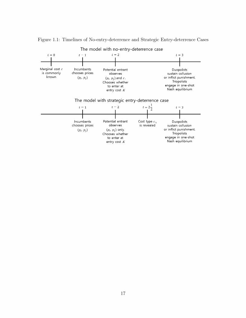
Figure 1.1: Timelines of No-entry-deterrence and Strategic Entry-deterrence Cases
17
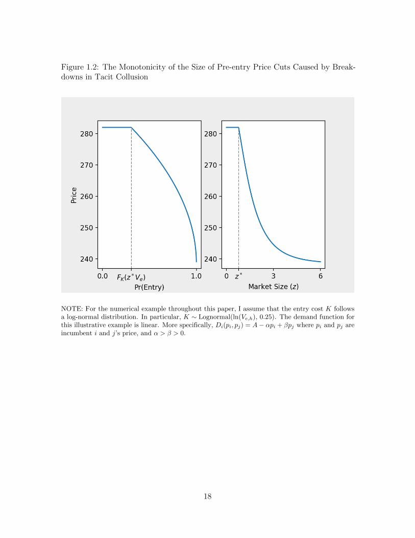
Figure 1.2: The Monotonicity of the Size of Pre-entry Price Cuts Caused by Break-downs in Tacit Collusion
NOTE: For the numerical example throughout this paper, I assume that the entry cost K followsa log-normal distribution. In particular, K ∼ Lognormal(ln(Ve,h), 0.25). The demand function forthis illustrative example is linear. More specifically, Di(pi, pj) = A− αpi + βpj where pi and pj areincumbent i and j’s price, and α > β > 0.
18
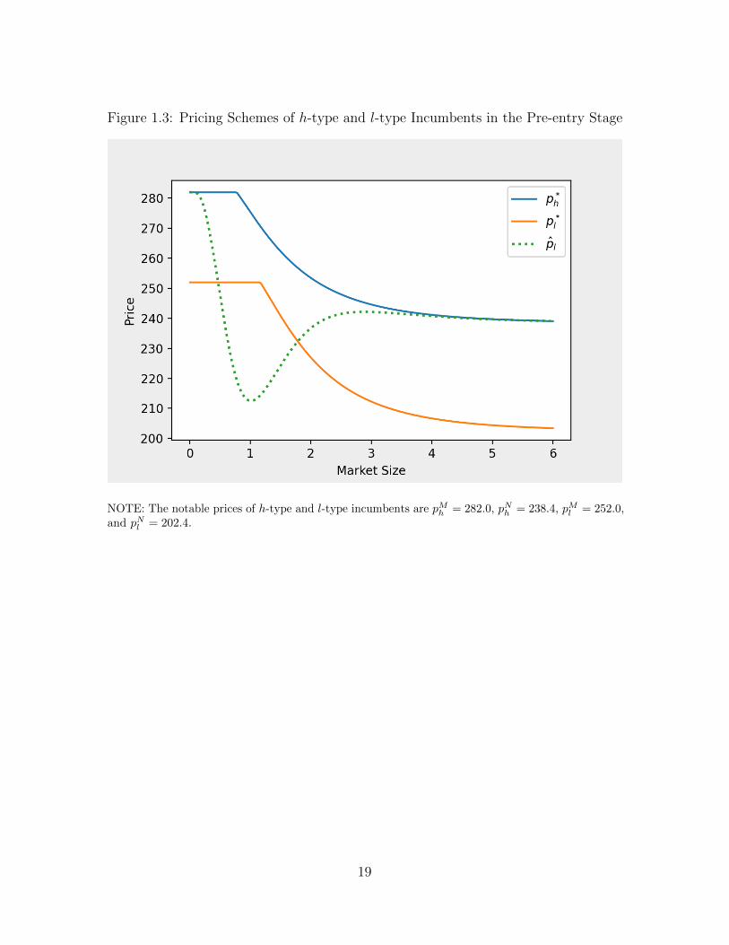
Figure 1.3: Pricing Schemes of h-type and l-type Incumbents in the Pre-entry Stage
NOTE: The notable prices of h-type and l-type incumbents are pMh = 282.0, pNh = 238.4, pMl = 252.0,and pNl = 202.4.
19
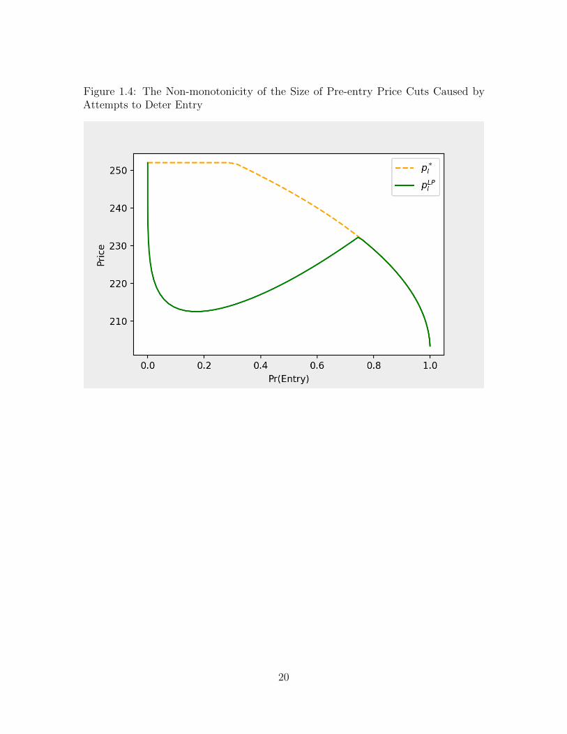
Figure 1.4: The Non-monotonicity of the Size of Pre-entry Price Cuts Caused byAttempts to Deter Entry
20
Chapter 2
Pre-entry Price Cutting by
Collusive Incumbents with an
Application to the Airline Industry
2.1 Introduction
Since Milgrom and Roberts’s (1982a) seminal work, economists have inves-
tigated incumbent firms’ strategic pricing in response to entry threat, called limit
pricing (pricing below the profit maximizing level even before entry occurs). Their
paper explain limit pricing as the preemptive behavior of an incumbent monopolist to
deter potential entry. Under asymmetric information about the incumbent’s marginal
costs, limit price may convince a potential rival that entry would be unprofitable and
eventually allow the monopolist to maintain monopoly profits continuously.
Following the spirit of Milgrom and Roberts (1982a), theoretical models have
studied oligopoly limit pricing (Harrington Jr, 1987; Bagwell and Ramey, 1991; Martin,
1995). As documented in Shin (2021a), however, those studies have not considered the
21
possibility of tacit collusion and how it can be the alternative explanation for pre-entry
price cutting. Shin (2021a) theoretically demonstrates that pre-entry price cutting
initiated by the threat of entry can be attributed to two motivations in oligopoly, a
breakdown in tacit collusion and an attempt to deter entry. The paper also provides
different testable predictions concerning incumbent oligopolists’ pre-entry price cuts.
Motivated by the testable predictions, this study empirically investigates
whether incumbent oligopolists’ pre-entry price cuts in the U.S. airline market are
more consistent with the prediction of a breakdown in tacit collusion or an attempt to
deter entry. The empirical model focuses on how ticket fares change after Southwest
Airlines becomes a potential entrant and how those changes are associated with the
estimated probability of entry. The model is estimated in two stages. In the first
stage, the entry probabilities are estimated with respect to market characteristics.
The second stage identifies the relationship between the pre-entry price cuts and the
estimated probability of entry. To this end, I use parametric and non-parametric
regression methods to determine whether the size of pre-entry price reductions is
monotonic or non-monotonic in the probability of entry.
The empirical investigation finds that incumbent oligopolists’ pre-entry price
reductions exhibit a more consistent pattern with a breakdown in tacit collusion. This
study’s test results reveal that the pre-entry price reductions appear larger as the
predicted probability of entry increases. This implies that the incumbent responses are
triggered by the reduced ability to sustain collusive prices, not by entry deterrence.
This paper continues as follows. Section 2.2 presents data sources for empirical
applications. Section 2.3 elaborates on the pre-entry price changes of incumbent
oligopolists in the airline industry. Section 2.4 provides descriptive tests to show that
incumbent oligopolists’ pre-entry price cuts are consistent with the implication of
breakdowns in tacit collusion. Using a hypothesis test, Section 2.5 shows that the
22
reduction patterns are monotonic in the estimated probability of entry in a more
robust way. Section 2.6 concludes.
2.2 Data and Sample Selection
The primary data sources of this study are the U.S. Department of Trans-
portation’s Airline Origin and Destination Survey (Databank 1, DB1) and its T-100
Domestic Segment (T100) from the first quarter of 1993 through the last quarter of
2017 (100 quarters). DB1 is a 10% sample randomly drawn from domestic itineraries
(100 passengers in DB1 implies 1,000 actual passengers). It includes itinerary fare,
origin and destination airport, round-trip, distance, and other itinerary-based details.
T100 is a supplement of DB1 such that it includes enplanement-based information
related to traffic at an airport, which is not captured in the itinerary-based DB1.1
It is well-known that several features in the airline industry facilitate collusion
between oligopoly carriers, such as public communication about capacity discipline
through earning calls (Aryal et al., 2017), rapid price communication through the
computer reservation systems (Borenstein, 2004), and multimarket contact (Bernheim
and Whinston, 1990; Evans and Kessides, 1994; Ciliberto and Williams, 2014). In
that sense, the empirical application using the airline industry data will provide better
insight into the responses to entry threats in markets where incumbents are tacitly
colluding.
A market is defined as a non-directional route between two endpoint airports. I
exclude markets from the sample where quarterly DB1 passengers (using either direct
or connecting flights) on average are less than 100.2 Also, the one-way distance of
1For example, I can figure out the number of flights and enplaned passenger traffic (possiblyincluding connecting passengers whose final destination is not one of the endpoints) at each endpointairport.
2Throughout this paper, one one-way passenger is counted as one DB1 passenger. Thus, one
23
markets in the sample should be at least 150 miles.
This study focuses on fares of incumbents’ direct flights. Incumbents’ itinerary
fares in DB1 can be aggregated to the passenger-weighted average fares at the carrier-
route-quarter level. The average fares will be used as the response variable in the
most empirical specifications. To remove noisy prices, I drop all itineraries in DB1
having questionable fare value based on Gerardi and Shapiro (2009).3
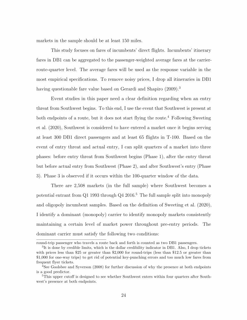
Event studies in this paper need a clear definition regarding when an entry
threat from Southwest begins. To this end, I use the event that Southwest is present at
both endpoints of a route, but it does not start flying the route.4 Following Sweeting
et al. (2020), Southwest is considered to have entered a market once it begins serving
at least 300 DB1 direct passengers and at least 65 flights in T-100. Based on the
event of entry threat and actual entry, I can split quarters of a market into three
phases: before entry threat from Southwest begins (Phase 1), after the entry threat
but before actual entry from Southwest (Phase 2), and after Southwest’s entry (Phase
3). Phase 3 is observed if it occurs within the 100-quarter window of the data.
There are 2,508 markets (in the full sample) where Southwest becomes a
potential entrant from Q1 1993 through Q4 2016.5 The full sample split into monopoly
and oligopoly incumbent samples. Based on the definition of Sweeting et al. (2020),
I identify a dominant (monopoly) carrier to identify monopoly markets consistently
maintaining a certain level of market power throughout pre-entry periods. The
dominant carrier must satisfy the following two conditions:
round-trip passenger who travels a route back and forth is counted as two DB1 passengers.3It is done by credible limits, which is the dollar credibility indicator in DB1. Also, I drop tickets
with prices less than $25 or greater than $2,000 for round-trips (less than $12.5 or greater than$1,000 for one-way trips) to get rid of potential key-punching errors and too much low fares fromfrequent flyer tickets.
4See Goolsbee and Syverson (2008) for further discussion of why the presence at both endpointsis a good predictor.
5This upper cutoff is designed to see whether Southwest enters within four quarters after South-west’s presence at both endpoints.
24
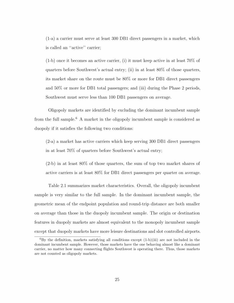
(1-a) a carrier must serve at least 300 DB1 direct passengers in a market, which
is called an ‘‘active’’ carrier;
(1-b) once it becomes an active carrier, (i) it must keep active in at least 70% of
quarters before Southwest’s actual entry; (ii) in at least 80% of those quarters,
its market share on the route must be 80% or more for DB1 direct passengers
and 50% or more for DB1 total passengers; and (iii) during the Phase 2 periods,
Southwest must serve less than 100 DB1 passengers on average.
Oligopoly markets are identified by excluding the dominant incumbent sample
from the full sample.6 A market in the oligopoly incumbent sample is considered as
duopoly if it satisfies the following two conditions:
(2-a) a market has active carriers which keep serving 300 DB1 direct passengers
in at least 70% of quarters before Southwest’s actual entry;
(2-b) in at least 80% of those quarters, the sum of top two market shares of
active carriers is at least 80% for DB1 direct passengers per quarter on average.
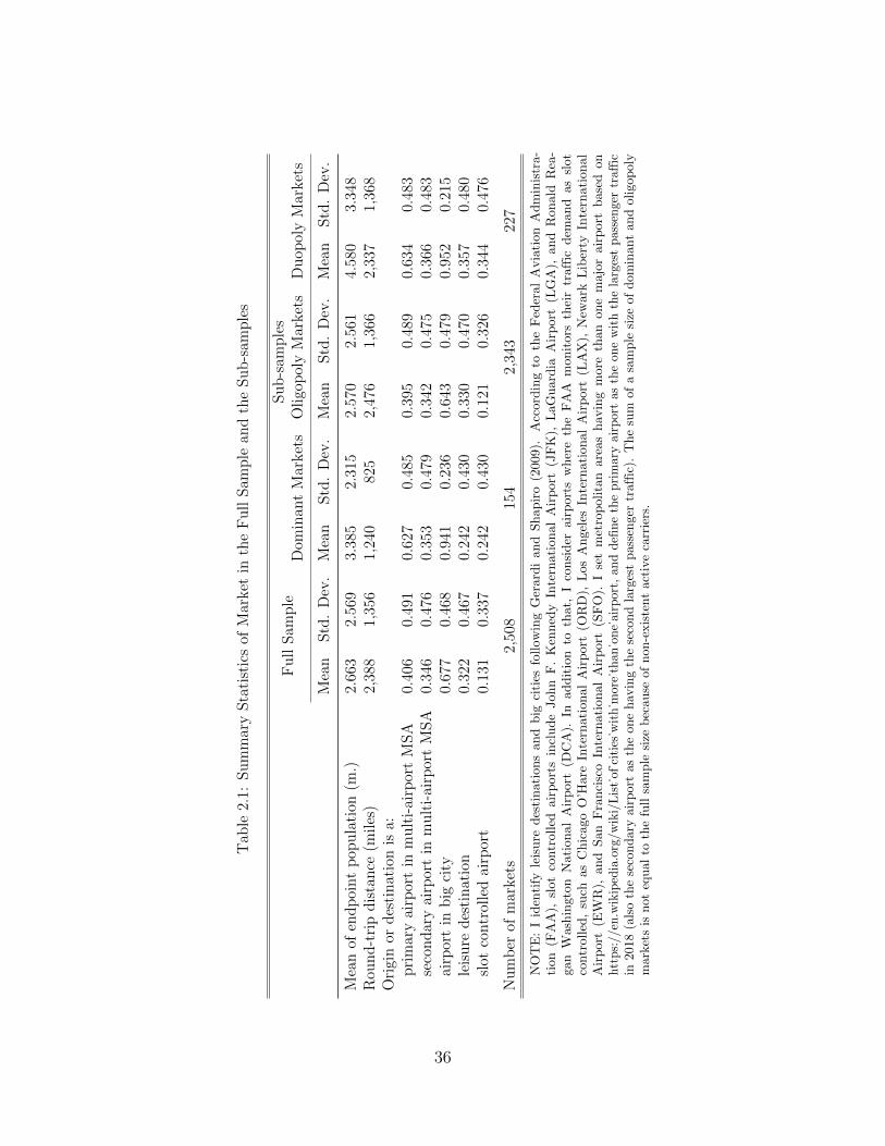
Table 2.1 summarizes market characteristics. Overall, the oligopoly incumbent
sample is very similar to the full sample. In the dominant incumbent sample, the
geometric mean of the endpoint population and round-trip distance are both smaller
on average than those in the duopoly incumbent sample. The origin or destination
features in duopoly markets are almost equivalent to the monopoly incumbent sample
except that duopoly markets have more leisure destinations and slot controlled airports.
6By the definition, markets satisfying all conditions except (1-b)(iii) are not included in thedominant incumbent sample. However, those markets have the one behaving almost like a dominantcarrier, no matter how many connecting flights Southwest is operating there. Thus, those marketsare not counted as oligopoly markets.
25
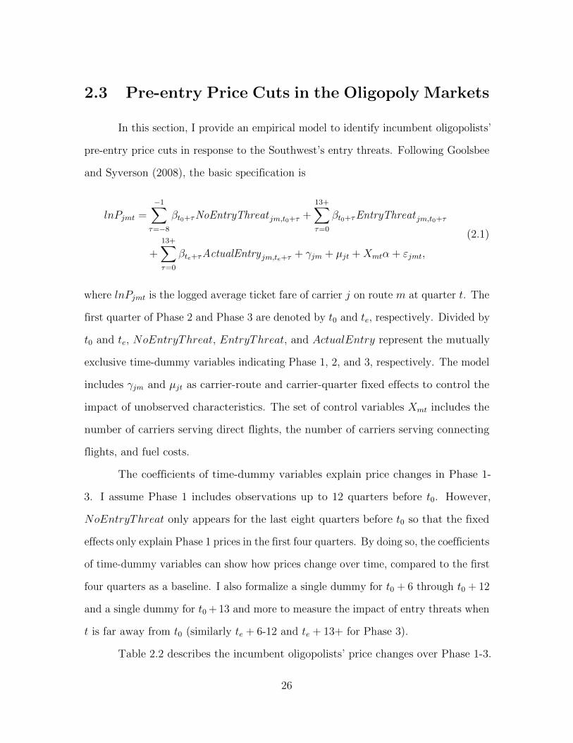
2.3 Pre-entry Price Cuts in the Oligopoly Markets
In this section, I provide an empirical model to identify incumbent oligopolists’
pre-entry price cuts in response to the Southwest’s entry threats. Following Goolsbee
and Syverson (2008), the basic specification is
lnPjmt =−1∑
τ=−8
βt0+τNoEntryThreat jm,t0+τ +13+∑τ=0
βt0+τEntryThreat jm,t0+τ
+13+∑τ=0
βte+τActualEntry jm,te+τ + γjm + µjt +Xmtα + εjmt,
(2.1)
where lnPjmt is the logged average ticket fare of carrier j on route m at quarter t. The
first quarter of Phase 2 and Phase 3 are denoted by t0 and te, respectively. Divided by
t0 and te, NoEntryThreat, EntryThreat, and ActualEntry represent the mutually
exclusive time-dummy variables indicating Phase 1, 2, and 3, respectively. The model
includes γjm and µjt as carrier-route and carrier-quarter fixed effects to control the
impact of unobserved characteristics. The set of control variables Xmt includes the
number of carriers serving direct flights, the number of carriers serving connecting
flights, and fuel costs.
The coefficients of time-dummy variables explain price changes in Phase 1-
3. I assume Phase 1 includes observations up to 12 quarters before t0. However,
NoEntryThreat only appears for the last eight quarters before t0 so that the fixed
effects only explain Phase 1 prices in the first four quarters. By doing so, the coefficients
of time-dummy variables can show how prices change over time, compared to the first
four quarters as a baseline. I also formalize a single dummy for t0 + 6 through t0 + 12
and a single dummy for t0 + 13 and more to measure the impact of entry threats when
t is far away from t0 (similarly te + 6-12 and te + 13+ for Phase 3).
Table 2.2 describes the incumbent oligopolists’ price changes over Phase 1-3.
26
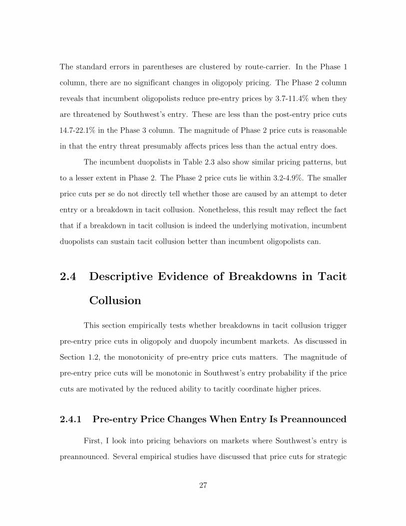
The standard errors in parentheses are clustered by route-carrier. In the Phase 1
column, there are no significant changes in oligopoly pricing. The Phase 2 column
reveals that incumbent oligopolists reduce pre-entry prices by 3.7-11.4% when they
are threatened by Southwest’s entry. These are less than the post-entry price cuts
14.7-22.1% in the Phase 3 column. The magnitude of Phase 2 price cuts is reasonable
in that the entry threat presumably affects prices less than the actual entry does.
The incumbent duopolists in Table 2.3 also show similar pricing patterns, but
to a lesser extent in Phase 2. The Phase 2 price cuts lie within 3.2-4.9%. The smaller
price cuts per se do not directly tell whether those are caused by an attempt to deter
entry or a breakdown in tacit collusion. Nonetheless, this result may reflect the fact
that if a breakdown in tacit collusion is indeed the underlying motivation, incumbent
duopolists can sustain tacit collusion better than incumbent oligopolists can.
2.4 Descriptive Evidence of Breakdowns in Tacit
Collusion
This section empirically tests whether breakdowns in tacit collusion trigger
pre-entry price cuts in oligopoly and duopoly incumbent markets. As discussed in
Section 1.2, the monotonicity of pre-entry price cuts matters. The magnitude of
pre-entry price cuts will be monotonic in Southwest’s entry probability if the price
cuts are motivated by the reduced ability to tacitly coordinate higher prices.
2.4.1 Pre-entry Price Changes When Entry Is Preannounced
First, I look into pricing behaviors on markets where Southwest’s entry is
preannounced. Several empirical studies have discussed that price cuts for strategic
27
entry deterrence could not be profitable when Southwest’s entry is inevitable (Dafny,
2005; Goolsbee and Syverson, 2008; Ellison and Ellison, 2011). On the other hand,
price declines caused by a breakdown in tacit collusion could still be observable even
though Southwest’s entry is preannounced.
Southwest typically releases a public announcement six months before the new
service begins. For example, Southwest posted on its media website in August 2011
that new service to Atlanta (ATL) is initiated in February 2012. On top of that,
Southwest reported new destinations to which they offer nonstop departures from ATL.
Since the existing carriers, flying between ATL and those destinations, knew that
Southwest’s entry was inevitable, they would not intend to deter the preannounced
entry.7 Using the observations of the preannounced markets, I examine the change of
pre-entry prices in response to actual entry across different market structures. The
empirical specification is
lnPjmt =−1∑
τ=−12
βte+τBeforeEntry jm,te+τ +13+∑τ=0
βte+τActualEntry jm,te+τ
+ γjm + µjt +Xmtα + εjmt,
(2.2)
where γjm and µjt are carrier-route and carrier-quarter fixed effects, respectively,
and Xmt are the control variables equivalent to the ones in equation (2.1). The
BeforeEntry time dummies include observations between te− 12 and te− 1, and the
ActualEntry time dummies represent observations after te.
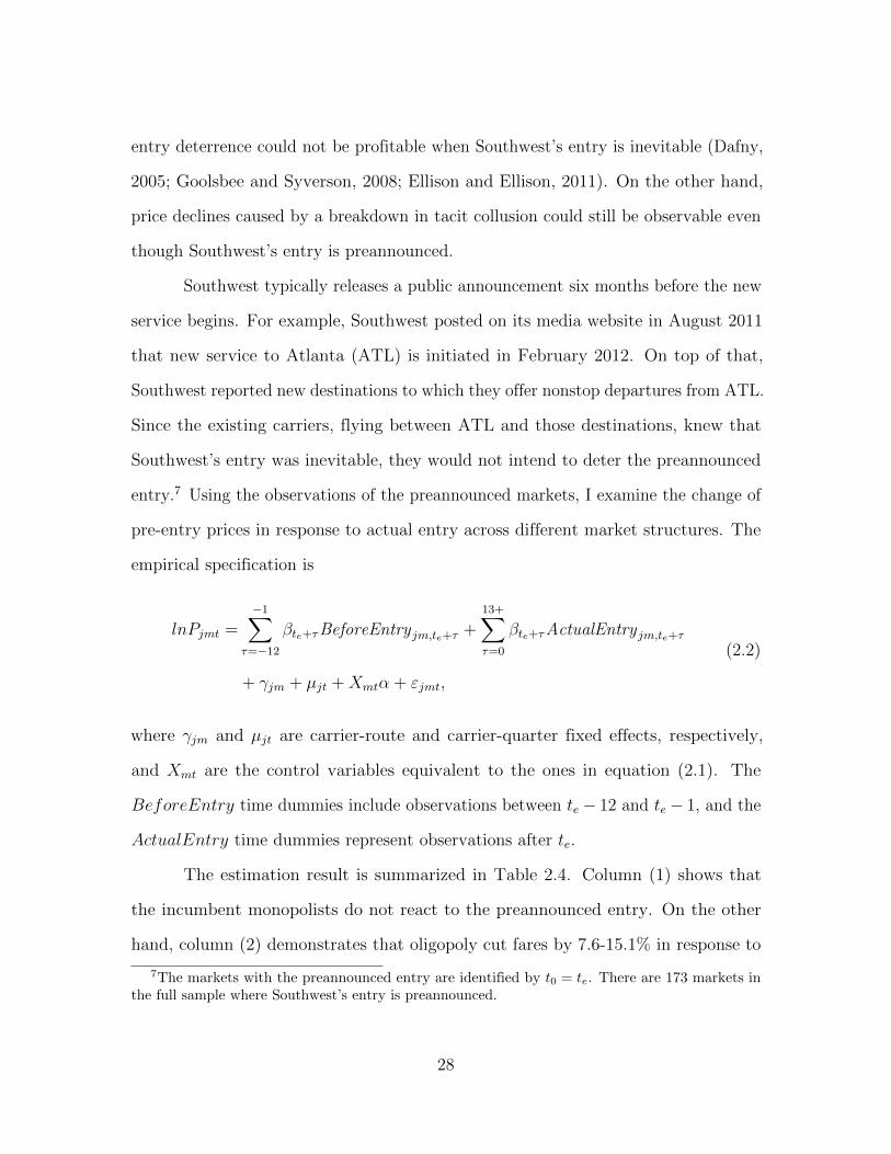
The estimation result is summarized in Table 2.4. Column (1) shows that
the incumbent monopolists do not react to the preannounced entry. On the other
hand, column (2) demonstrates that oligopoly cut fares by 7.6-15.1% in response to
7The markets with the preannounced entry are identified by t0 = te. There are 173 markets inthe full sample where Southwest’s entry is preannounced.
28
the preannounced entry. Even though the pre-entry price cuts are not consistent
throughout the entire periods, a F test shows that all coefficients of te − 12 through
te − 1 are significantly different from zero with a p-value of 0.008. The empirical
specification is also applied to duopoly markets and markets with more than two
firms. Based on columns (3) and (4), one can notice that the pre-entry price cuts in
column (2) mostly come from markets with more than two firms. In column (4), a
F test on the coefficients of te − 12 through te − 1 shows that they are significantly
different from zero with a p-value of 0.030.
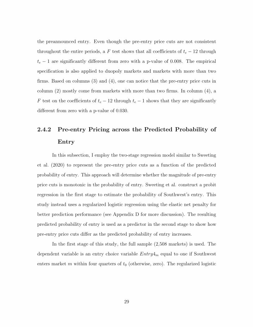
2.4.2 Pre-entry Pricing across the Predicted Probability of
Entry
In this subsection, I employ the two-stage regression model similar to Sweeting
et al. (2020) to represent the pre-entry price cuts as a function of the predicted
probability of entry. This approach will determine whether the magnitude of pre-entry
price cuts is monotonic in the probability of entry. Sweeting et al. construct a probit
regression in the first stage to estimate the probability of Southwest’s entry. This
study instead uses a regularized logistic regression using the elastic net penalty for
better prediction performance (see Appendix D for more discussion). The resulting
predicted probability of entry is used as a predictor in the second stage to show how
pre-entry price cuts differ as the predicted probability of entry increases.
In the first stage of this study, the full sample (2,508 markets) is used. The
dependent variable is an entry choice variable Entry4m equal to one if Southwest
enters market m within four quarters of t0 (otherwise, zero). The regularized logistic
29
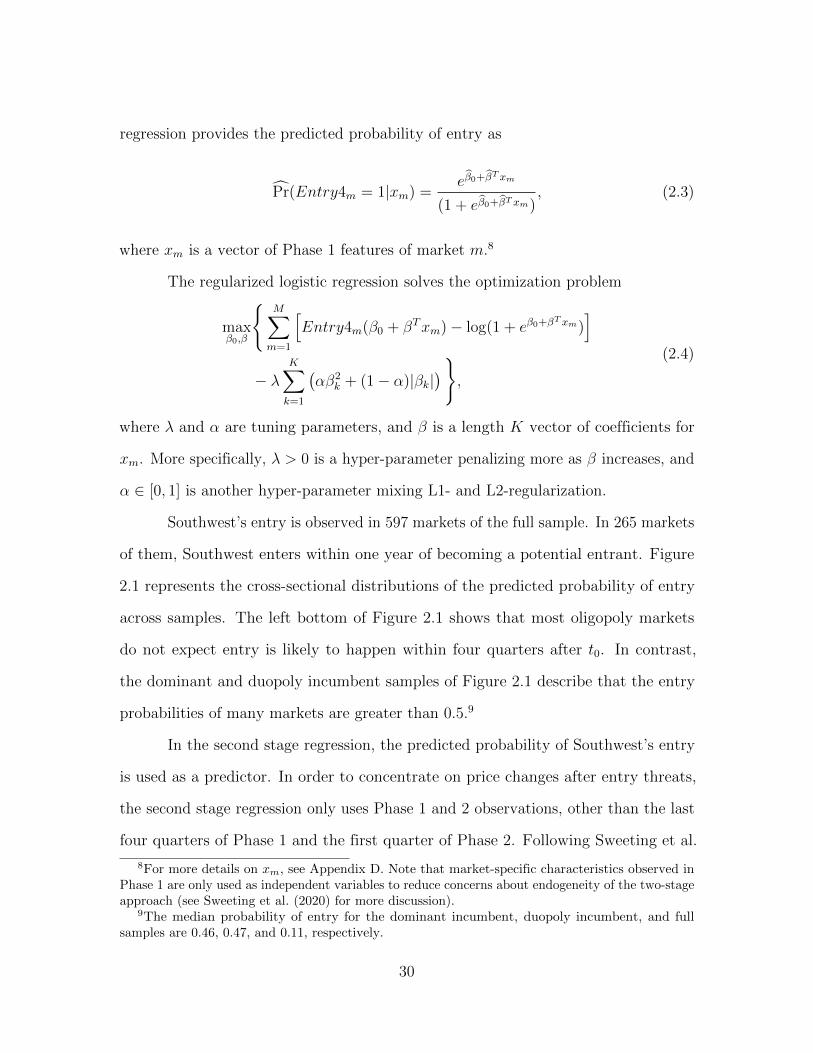
regression provides the predicted probability of entry as
Pr(Entry4m = 1|xm) =eβ0+β
T xm
(1 + eβ0+βT xm), (2.3)
where xm is a vector of Phase 1 features of market m.8
The regularized logistic regression solves the optimization problem
(2.4)
maxβ0,β
{M∑m=1
[Entry4m(β0 + βTxm)− log(1 + eβ0+β
T xm)]
− λK∑k=1
(αβ2
k + (1− α)|βk|)}
,
where λ and α are tuning parameters, and β is a length K vector of coefficients for
xm. More specifically, λ > 0 is a hyper-parameter penalizing more as β increases, and
α ∈ [0, 1] is another hyper-parameter mixing L1- and L2-regularization.
Southwest’s entry is observed in 597 markets of the full sample. In 265 markets
of them, Southwest enters within one year of becoming a potential entrant. Figure
2.1 represents the cross-sectional distributions of the predicted probability of entry
across samples. The left bottom of Figure 2.1 shows that most oligopoly markets
do not expect entry is likely to happen within four quarters after t0. In contrast,
the dominant and duopoly incumbent samples of Figure 2.1 describe that the entry
probabilities of many markets are greater than 0.5.9
In the second stage regression, the predicted probability of Southwest’s entry
is used as a predictor. In order to concentrate on price changes after entry threats,
the second stage regression only uses Phase 1 and 2 observations, other than the last
four quarters of Phase 1 and the first quarter of Phase 2. Following Sweeting et al.
8For more details on xm, see Appendix D. Note that market-specific characteristics observed inPhase 1 are only used as independent variables to reduce concerns about endogeneity of the two-stageapproach (see Sweeting et al. (2020) for more discussion).
9The median probability of entry for the dominant incumbent, duopoly incumbent, and fullsamples are 0.46, 0.47, and 0.11, respectively.
30
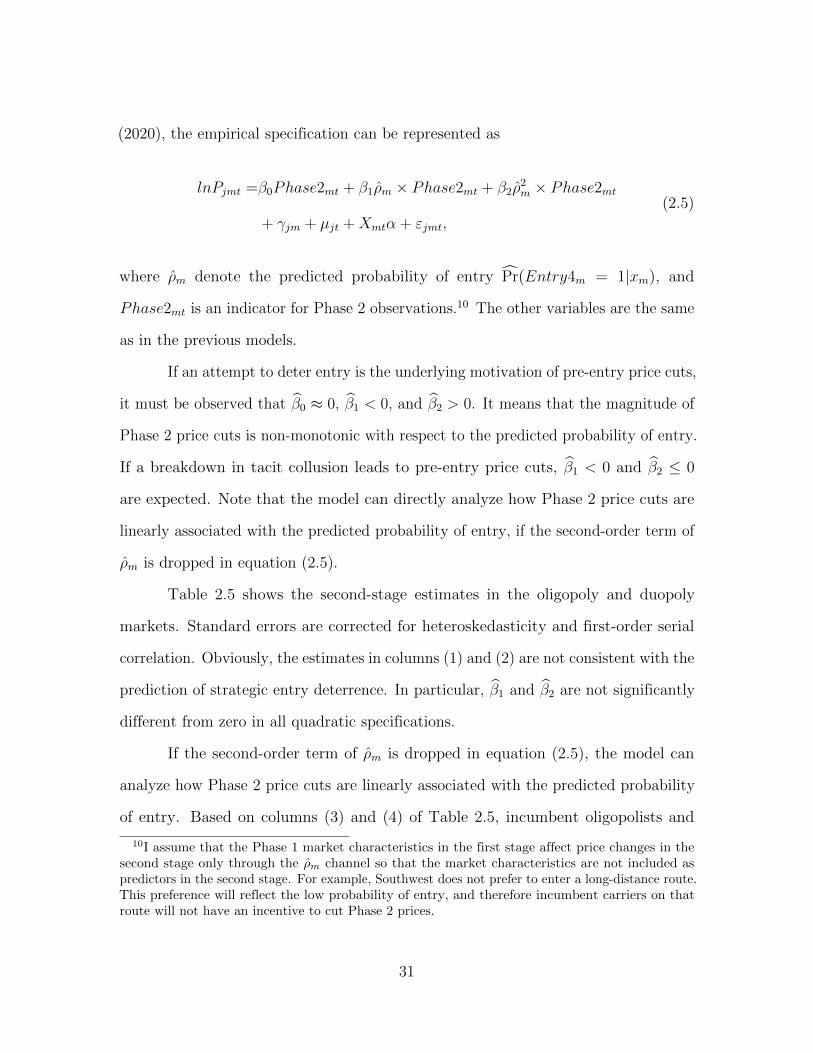
(2020), the empirical specification can be represented as
lnPjmt =β0Phase2mt + β1ρm × Phase2mt + β2ρ2m × Phase2mt
+ γjm + µjt +Xmtα + εjmt,
(2.5)
where ρm denote the predicted probability of entry Pr(Entry4m = 1|xm), and
Phase2mt is an indicator for Phase 2 observations.10 The other variables are the same
as in the previous models.
If an attempt to deter entry is the underlying motivation of pre-entry price cuts,
it must be observed that β0 ≈ 0, β1 < 0, and β2 > 0. It means that the magnitude of
Phase 2 price cuts is non-monotonic with respect to the predicted probability of entry.
If a breakdown in tacit collusion leads to pre-entry price cuts, β1 < 0 and β2 ≤ 0
are expected. Note that the model can directly analyze how Phase 2 price cuts are
linearly associated with the predicted probability of entry, if the second-order term of
ρm is dropped in equation (2.5).
Table 2.5 shows the second-stage estimates in the oligopoly and duopoly
markets. Standard errors are corrected for heteroskedasticity and first-order serial
correlation. Obviously, the estimates in columns (1) and (2) are not consistent with the
prediction of strategic entry deterrence. In particular, β1 and β2 are not significantly
different from zero in all quadratic specifications.
If the second-order term of ρm is dropped in equation (2.5), the model can
analyze how Phase 2 price cuts are linearly associated with the predicted probability
of entry. Based on columns (3) and (4) of Table 2.5, incumbent oligopolists and
10I assume that the Phase 1 market characteristics in the first stage affect price changes in thesecond stage only through the ρm channel so that the market characteristics are not included aspredictors in the second stage. For example, Southwest does not prefer to enter a long-distance route.This preference will reflect the low probability of entry, and therefore incumbent carriers on thatroute will not have an incentive to cut Phase 2 prices.
31
duopolists reduce more prices in Phase 2 as the predicted probability of entry rises.
These reduction patterns are more consistent with the prediction of a breakdown in
tacit collusion. Figure 2.2 illustrates the linear relationship between ρm and the Phase
2 price cuts. The largest estimated price falls are 8.5% and 7.6% in oligopoly and
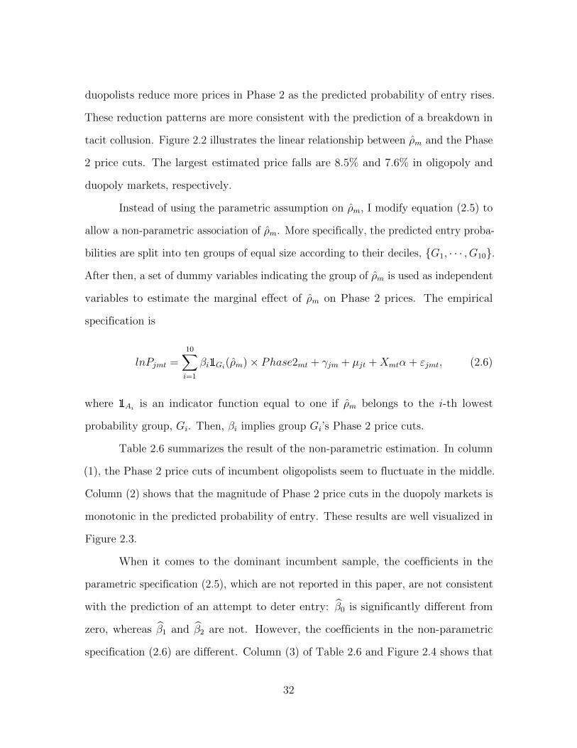
duopoly markets, respectively.
Instead of using the parametric assumption on ρm, I modify equation (2.5) to
allow a non-parametric association of ρm. More specifically, the predicted entry proba-
bilities are split into ten groups of equal size according to their deciles, {G1, · · · , G10}.
After then, a set of dummy variables indicating the group of ρm is used as independent
variables to estimate the marginal effect of ρm on Phase 2 prices. The empirical
specification is
lnPjmt =10∑i=1
βi1Gi(ρm)× Phase2mt + γjm + µjt +Xmtα + εjmt, (2.6)
where 1Aiis an indicator function equal to one if ρm belongs to the i-th lowest
probability group, Gi. Then, βi implies group Gi’s Phase 2 price cuts.
Table 2.6 summarizes the result of the non-parametric estimation. In column
(1), the Phase 2 price cuts of incumbent oligopolists seem to fluctuate in the middle.
Column (2) shows that the magnitude of Phase 2 price cuts in the duopoly markets is
monotonic in the predicted probability of entry. These results are well visualized in
Figure 2.3.
When it comes to the dominant incumbent sample, the coefficients in the
parametric specification (2.5), which are not reported in this paper, are not consistent
with the prediction of an attempt to deter entry: β0 is significantly different from
zero, whereas β1 and β2 are not. However, the coefficients in the non-parametric
specification (2.6) are different. Column (3) of Table 2.6 and Figure 2.4 shows that
32

the biggest price drop occurs in the middle of the probability groups. Also, it becomes
closer to zero when entry is extremely likely. This may imply that the dominant
incumbents engage in limit pricing.
2.5 Hypothesis Testing for Monotonicity
In this section, I use a hypothesis test in Ellison and Ellison (2011), initially
developed by Hall and Heckman (2000), to address the monotonicity of incumbent
oligopolists’ pre-entry price cuts in a more robust way. The idea of Ellison and
Ellison’s test is related to the notion of running gradients: if a response variable is
non-monotonically associated with data points, one is likely to find subsets of the
data points on which a linear regression has both positive and negative gradients. To
this end, I construct the data generating process of the form
lnPjmt = β0Phase2mt + β1ρm × Phase2mt + γjm + µjt +Xmtα + εjmt, (2.7)
which is the linear form of the second-stage regression in equation (2.5). Of course, β1
illustrates how the pre-entry price cut is linearly associated with ρm.
Let R ⊂ [0, 1] denote a closed interval over which the running gradients will
be computed for Ellison and Ellison’s test. Then, the subset of the ρm’s can be
represented as P = R∩ {ρ1, ρ2, · · · , ρM}, where M is the number of markets. Their
test statistic for monotonicity is
TEE = min
{max
{R:|P|≥M}−βP1 σPρ , max
{R:|P|≥M}βP1 σ
Pρ
}. (2.8)
Note that P should have at least M number of the ρm’s.11 Let βP1 denote the estimator
11In particular, M = 1.5(logM)2. Based on Hall and Heckman (2000), the effects of outlying data
33
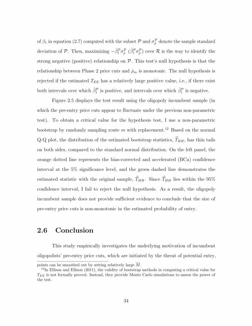
of β1 in equation (2.7) computed with the subset P and σPρ denote the sample standard
deviation of P . Then, maximizing −βP1 σPρ (βP1 σPρ ) over R is the way to identify the
strong negative (positive) relationship on P. This test’s null hypothesis is that the
relationship between Phase 2 price cuts and ρm is monotonic. The null hypothesis is
rejected if the estimated TEE has a relatively large positive value, i.e., if there exist
both intervals over which βP1 is positive, and intervals over which βP1 is negative.
Figure 2.5 displays the test result using the oligopoly incumbent sample (in
which the pre-entry price cuts appear to fluctuate under the previous non-parametric
test). To obtain a critical value for the hypothesis test, I use a non-parametric
bootstrap by randomly sampling route m with replacement.12 Based on the normal
Q-Q plot, the distribution of the estimated bootstrap statistics, THH , has thin tails
on both sides, compared to the standard normal distribution. On the left panel, the
orange dotted line represents the bias-corrected and accelerated (BCa) confidence
interval at the 5% significance level, and the green dashed line demonstrates the
estimated statistic with the original sample, THH . Since THH lies within the 95%
confidence interval, I fail to reject the null hypothesis. As a result, the oligopoly
incumbent sample does not provide sufficient evidence to conclude that the size of
pre-entry price cuts is non-monotonic in the estimated probability of entry.
2.6 Conclusion
This study empirically investigates the underlying motivation of incumbent
oligopolists’ pre-entry price cuts, which are initiated by the threat of potential entry,
points can be smoothed out by setting relatively large M .12In Ellison and Ellison (2011), the validity of bootstrap methods in computing a critical value for
TEE is not formally proved. Instead, they provide Monte Carlo simulations to assess the power ofthe test.
34
in the U.S. airline market: whether the price cuts are driven by a breakdown in tacit
collusion or an attempt to deter entry. To this end, the testable predictions regarding
the price reduction patterns in Shin (2021a) are used. The empirical model focuses on
how ticket fares change after Southwest Airlines becomes a potential entrant and how
those changes are associated with the estimated probability of entry.
I employ a two-stage model to test the relationship between the price drops
and the likelihood of entry. In the first stage, the entry probabilities are estimated
with a regularized logistic regression, which shows better prediction performances. In
the second stage, I construct parametric and non-parametric regression models using
the predicted probability of entry as a predictor variable to determine whether the
reduction patterns of pre-entry prices are consistent with the prediction of breakdowns
in tacit collusion or strategic entry deterrence.
The two-stage model provides a basis for empirical tests examining the underly-
ing motivation for incumbents’ pre-entry price cuts. The descriptive tests indicate that
the magnitude of pre-entry price reductions is monotonic in the predicted probability
of Southwest’s entry. It implies that the underlying motivation is more consistent
with the prediction of a breakdown in tacit collusion. Sweeting et al. (2020) show that
pre-entry price cuts of dominant incumbent carriers are attributed to an attempt to
deter entry. However, this paper’s empirical tests do not provide consistent evidence
that strategic entry deterrence is the underlying motivation.
35
Tab
le2.
1:S
um
mar
yS
tati
stic
sof
Mar
ket
inth
eF
ull
Sam
ple
and
the
Su
b-s
amp
les
Fu
llS
amp
leS
ub
-sam
ple
sD
omin
ant
Mar
ket
sO
ligo
pol
yM
arket
sD
uop
oly
Mar
ket
s
Mea
nS
td.
Dev
.M
ean
Std
.D
ev.
Mea
nS
td.
Dev
.M
ean
Std
.D
ev.
Mea
nof
end
poi
nt
pop
ula
tion
(m.)
2.66
32.
569
3.38
52.
315
2.57
02.
561
4.58
03.
348
Rou
nd
-tri
pd
ista
nce
(mil
es)
2,38
81,
356
1,24
082
52,
476
1,36
62,
337
1,36
8O
rigi
nor
des
tinat
ion
isa:
pri
mar
yai
rpor
tin
mu
lti-
airp
ort
MS
A0.
406
0.49
10.
627
0.48
50.
395
0.48
90.
634
0.48
3se
con
dar
yai
rpor
tin
mu
lti-
airp
ort
MS
A0.
346
0.47
60.
353
0.47
90.
342
0.47
50.
366
0.48
3ai
rpor
tin
big
city
0.67
70.
468
0.94
10.
236
0.64
30.
479
0.95
20.
215
leis
ure
des
tin
atio
n0.
322
0.46
70.
242
0.43
00.
330
0.47
00.
357
0.48
0sl
otco
ntr
olle
dai
rpor
t0.
131
0.33
70.
242
0.43
00.
121
0.32
60.
344
0.47
6
Nu
mb
erof
mar
ket
s2,
508
154
2,34
322
7
NOTE:Iidentify
leisure
destinationsandbig
cities
followingGerardiandShapiro(2009).
Accordingto
theFederalAviationAdministra-
tion
(FAA),
slotcontrolled
airportsincludeJohn
F.KennedyInternationalAirport
(JFK),
LaGuardia
Airport
(LGA),
and
Ronald
Rea-
gan
Washington
NationalAirport
(DCA).
Inaddition
tothat,
Iconsider
airportswheretheFAA
monitors
theirtraffic
dem
and
asslot
controlled,such
asChicagoO’H
are
InternationalAirport
(ORD),
LosAngeles
InternationalAirport
(LAX),
New
ark
Liberty
International
Airport
(EW
R),
and
San
FranciscoInternationalAirport
(SFO).
Isetmetropolitan
areashavingmore
than
onemajorairport
based
on
https://en.wikipedia.org/w
iki/List˙of˙cities˙with˙m
ore˙than
˙one˙airport,
anddefinetheprimaryairportas
theon
ewiththelargestpassengertraffic
in2018(alsothesecondary
airport
astheonehavingthesecondlargestpassenger
traffic).
Thesum
ofasample
size
ofdominantandoligopoly
marketsis
not
equal
tothefullsample
size
becau
seof
non
-existentactivecarriers.
36
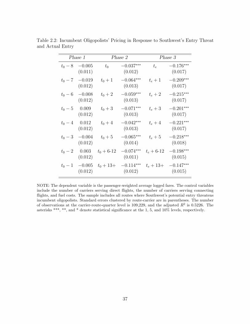
Table 2.2: Incumbent Oligopolists’ Pricing in Response to Southwest’s Entry Threatand Actual Entry
Phase 1 Phase 2 Phase 3
t0 − 8 −0.005 t0 −0.037∗∗∗ te −0.176∗∗∗
(0.011) (0.012) (0.017)
t0 − 7 −0.019 t0 + 1 −0.064∗∗∗ te + 1 −0.209∗∗∗
(0.012) (0.013) (0.017)
t0 − 6 −0.008 t0 + 2 −0.059∗∗∗ te + 2 −0.215∗∗∗
(0.012) (0.013) (0.017)
t0 − 5 0.009 t0 + 3 −0.071∗∗∗ te + 3 −0.201∗∗∗
(0.012) (0.013) (0.017)
t0 − 4 0.012 t0 + 4 −0.042∗∗∗ te + 4 −0.221∗∗∗
(0.012) (0.013) (0.017)
t0 − 3 −0.004 t0 + 5 −0.065∗∗∗ te + 5 −0.218∗∗∗
(0.012) (0.014) (0.018)
t0 − 2 0.003 t0 + 6-12 −0.074∗∗∗ te + 6-12 −0.198∗∗∗
(0.012) (0.011) (0.015)
t0 − 1 −0.005 t0 + 13+ −0.114∗∗∗ te + 13+ −0.147∗∗∗
(0.012) (0.012) (0.015)
NOTE: The dependent variable is the passenger-weighted average logged fares. The control variablesinclude the number of carriers serving direct flights, the number of carriers serving connectingflights, and fuel costs. The sample includes all routes where Southwest’s potential entry threatensincumbent oligopolists. Standard errors clustered by route-carrier are in parentheses. The numberof observations at the carrier-route-quarter level is 109,229, and the adjusted R2 is 0.5226. Theasterisks ***, **, and * denote statistical significance at the 1, 5, and 10% levels, respectively.
37
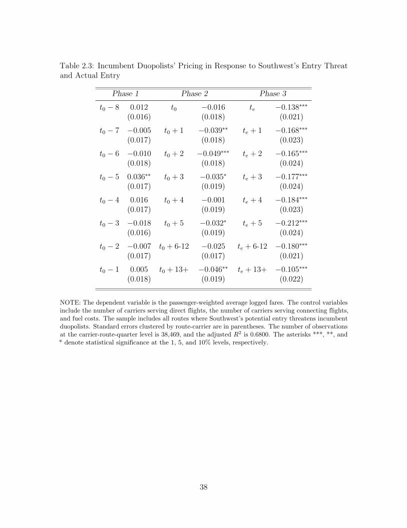
Table 2.3: Incumbent Duopolists’ Pricing in Response to Southwest’s Entry Threatand Actual Entry
Phase 1 Phase 2 Phase 3
t0 − 8 0.012 t0 −0.016 te −0.138∗∗∗
(0.016) (0.018) (0.021)
t0 − 7 −0.005 t0 + 1 −0.039∗∗ te + 1 −0.168∗∗∗
(0.017) (0.018) (0.023)
t0 − 6 −0.010 t0 + 2 −0.049∗∗∗ te + 2 −0.165∗∗∗
(0.018) (0.018) (0.024)
t0 − 5 0.036∗∗ t0 + 3 −0.035∗ te + 3 −0.177∗∗∗
(0.017) (0.019) (0.024)
t0 − 4 0.016 t0 + 4 −0.001 te + 4 −0.184∗∗∗
(0.017) (0.019) (0.023)
t0 − 3 −0.018 t0 + 5 −0.032∗ te + 5 −0.212∗∗∗
(0.016) (0.019) (0.024)
t0 − 2 −0.007 t0 + 6-12 −0.025 te + 6-12 −0.180∗∗∗
(0.017) (0.017) (0.021)
t0 − 1 0.005 t0 + 13+ −0.046∗∗ te + 13+ −0.105∗∗∗
(0.018) (0.019) (0.022)
NOTE: The dependent variable is the passenger-weighted average logged fares. The control variablesinclude the number of carriers serving direct flights, the number of carriers serving connecting flights,and fuel costs. The sample includes all routes where Southwest’s potential entry threatens incumbentduopolists. Standard errors clustered by route-carrier are in parentheses. The number of observationsat the carrier-route-quarter level is 38,469, and the adjusted R2 is 0.6800. The asterisks ***, **, and* denote statistical significance at the 1, 5, and 10% levels, respectively.
38
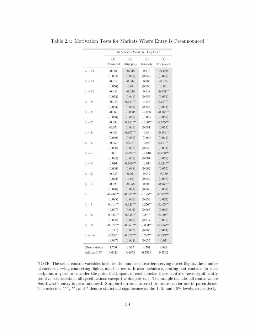
Table 2.4: Motivation Tests for Markets Where Entry Is Preannounced
Dependent Variable: Log Price
(1) (2) (3) (4)
Dominant Oligopoly Duopoly Triopoly+
te − 12 -0.081 -0.038 0.019 -0.109
(0.064) (0.046) (0.052) (0.075)
te − 11 -0.014 -0.044 0.006 -0.074
(0.056) (0.04) (0.056) (0.06)
te − 10 -0.046 -0.059 0.048 -0.137∗∗
(0.072) (0.041) (0.055) (0.059)
te − 9 -0.046 -0.114∗∗∗ -0.100∗ -0.157∗∗∗
(0.063) (0.039) (0.053) (0.061)
te − 8 -0.069 -0.083∗ -0.036 -0.136∗∗
(0.056) (0.046) (0.06) (0.067)
te − 7 -0.032 -0.151∗∗∗ -0.160∗∗∗ -0.175∗∗∗
(0.07) (0.041) (0.051) (0.063)
te − 6 -0.086 -0.107∗∗∗ -0.091 -0.154∗∗
(0.069) (0.039) (0.06) (0.061)
te − 5 -0.053 -0.076∗∗ -0.037 -0.177∗∗∗
(0.068) (0.037) (0.055) (0.051)
te − 4 0.001 -0.090∗∗ -0.010 -0.188∗∗∗
(0.064) (0.045) (0.061) (0.069)
te − 3 0.016 -0.100∗∗∗ -0.011 -0.224∗∗∗
(0.069) (0.038) (0.062) (0.055)
te − 2 -0.039 -0.004 0.042 -0.089
(0.072) (0.04) (0.055) (0.059)
te − 1 -0.020 -0.058 0.005 -0.135∗∗
(0.076) (0.043) (0.065) (0.061)
te -0.249∗∗∗ -0.272∗∗∗ -0.175∗∗∗ -0.367∗∗∗
(0.085) (0.046) (0.059) (0.074)
te + 1 -0.414∗∗∗ -0.323∗∗∗ -0.250∗∗∗ -0.405∗∗∗
(0.097) (0.046) (0.063) (0.069)
te + 2 -0.443∗∗∗ -0.345∗∗∗ -0.257∗∗∗ -0.459∗∗∗
(0.098) (0.046) (0.077) (0.067)
te + 3 -0.372∗∗∗ -0.351∗∗∗ -0.303∗∗∗ -0.415∗∗∗
(0.111) (0.047) (0.066) (0.074)
te + 4+ -0.230∗∗ -0.315∗∗∗ -0.222∗∗∗ -0.393∗∗∗
(0.097) (0.043) (0.055) (0.07)
Observations 1,706 9,867 4,797 4,893
Adjusted R2 0.6343 0.6658 0.7519 0.5592
NOTE: The set of control variables includes the number of carriers serving direct flights, the numberof carriers serving connecting flights, and fuel costs. It also includes operating cost controls for eachendpoint airport to consider the potential impact of cost shocks: these controls have significantlypositive coefficients in all specifications except the duopoly one. The sample includes all routes whereSouthwest’s entry is preannounced. Standard errors clustered by route-carrier are in parentheses.The asterisks ***, **, and * denote statistical significance at the 1, 5, and 10% levels, respectively.
39
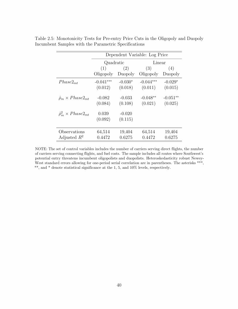
Table 2.5: Monotonicity Tests for Pre-entry Price Cuts in the Oligopoly and DuopolyIncumbent Samples with the Parametric Specifications
Dependent Variable: Log Price
Quadratic Linear(1) (2) (3) (4)
Oligopoly Duopoly Oligopoly Duopoly
Phase2mt -0.041∗∗∗ -0.030∗ -0.044∗∗∗ -0.029∗
(0.012) (0.018) (0.011) (0.015)
ρm × Phase2mt -0.082 -0.033 -0.048∗∗ -0.051∗∗
(0.084) (0.108) (0.021) (0.025)
ρ2m × Phase2mt 0.039 -0.020(0.092) (0.115)
Observations 64,514 19,404 64,514 19,404Adjusted R2 0.4472 0.6275 0.4472 0.6275
NOTE: The set of control variables includes the number of carriers serving direct flights, the numberof carriers serving connecting flights, and fuel costs. The sample includes all routes where Southwest’spotential entry threatens incumbent oligopolists and duopolists. Heteroskedasticity robust Newey-West standard errors allowing for one-period serial correlation are in parentheses. The asterisks ***,**, and * denote statistical significance at the 1, 5, and 10% levels, respectively.
40
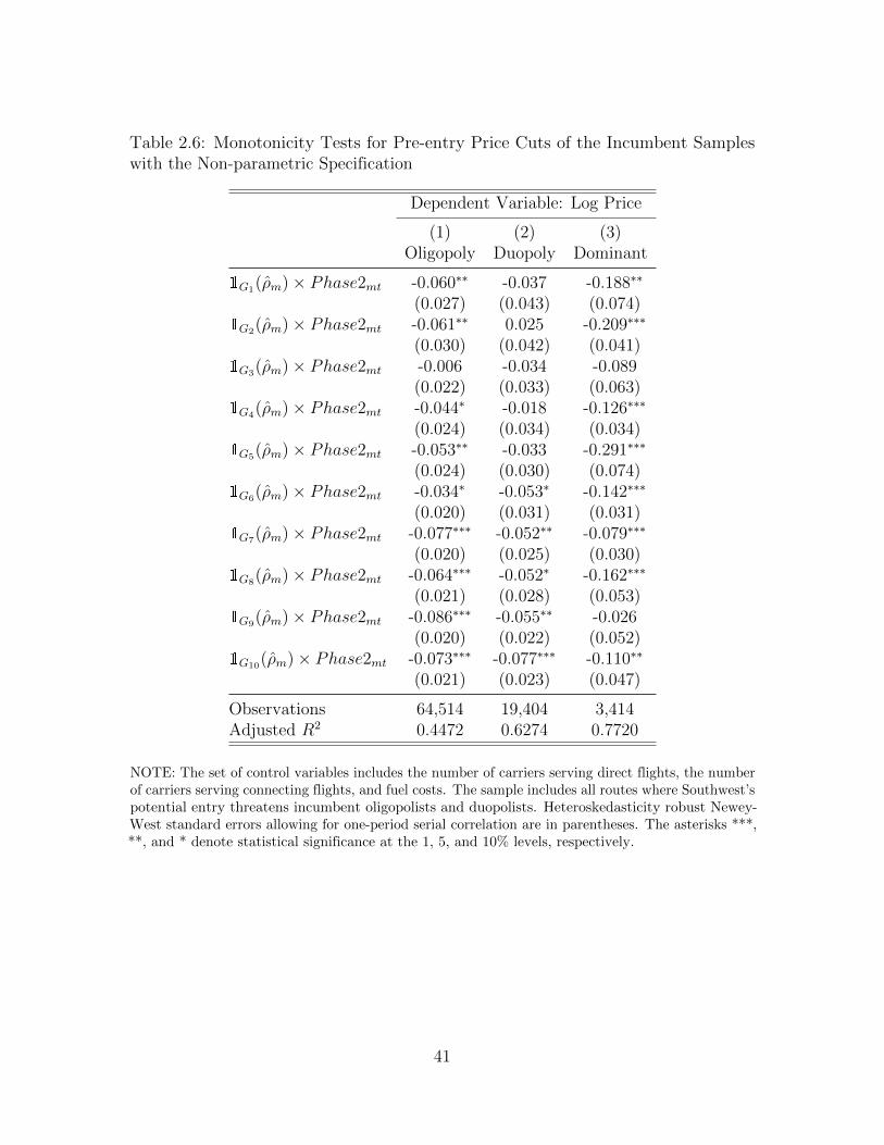
Table 2.6: Monotonicity Tests for Pre-entry Price Cuts of the Incumbent Sampleswith the Non-parametric Specification
Dependent Variable: Log Price
(1) (2) (3)Oligopoly Duopoly Dominant
1G1(ρm)× Phase2mt -0.060∗∗ -0.037 -0.188∗∗
(0.027) (0.043) (0.074)1G2(ρm)× Phase2mt -0.061∗∗ 0.025 -0.209∗∗∗
(0.030) (0.042) (0.041)1G3(ρm)× Phase2mt -0.006 -0.034 -0.089
(0.022) (0.033) (0.063)1G4(ρm)× Phase2mt -0.044∗ -0.018 -0.126∗∗∗
(0.024) (0.034) (0.034)1G5(ρm)× Phase2mt -0.053∗∗ -0.033 -0.291∗∗∗
(0.024) (0.030) (0.074)1G6(ρm)× Phase2mt -0.034∗ -0.053∗ -0.142∗∗∗
(0.020) (0.031) (0.031)1G7(ρm)× Phase2mt -0.077∗∗∗ -0.052∗∗ -0.079∗∗∗
(0.020) (0.025) (0.030)1G8(ρm)× Phase2mt -0.064∗∗∗ -0.052∗ -0.162∗∗∗
(0.021) (0.028) (0.053)1G9(ρm)× Phase2mt -0.086∗∗∗ -0.055∗∗ -0.026
(0.020) (0.022) (0.052)1G10(ρm)× Phase2mt -0.073∗∗∗ -0.077∗∗∗ -0.110∗∗
(0.021) (0.023) (0.047)
Observations 64,514 19,404 3,414Adjusted R2 0.4472 0.6274 0.7720
NOTE: The set of control variables includes the number of carriers serving direct flights, the numberof carriers serving connecting flights, and fuel costs. The sample includes all routes where Southwest’spotential entry threatens incumbent oligopolists and duopolists. Heteroskedasticity robust Newey-West standard errors allowing for one-period serial correlation are in parentheses. The asterisks ***,**, and * denote statistical significance at the 1, 5, and 10% levels, respectively.
41
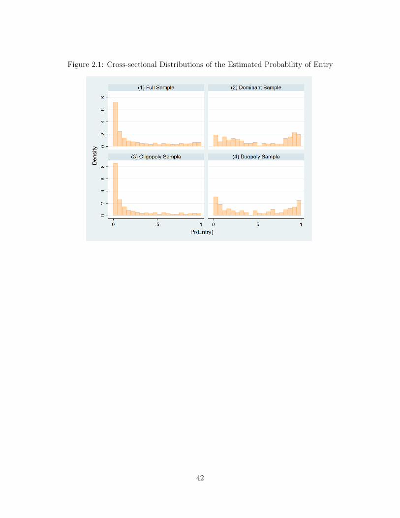
Figure 2.1: Cross-sectional Distributions of the Estimated Probability of Entry
42
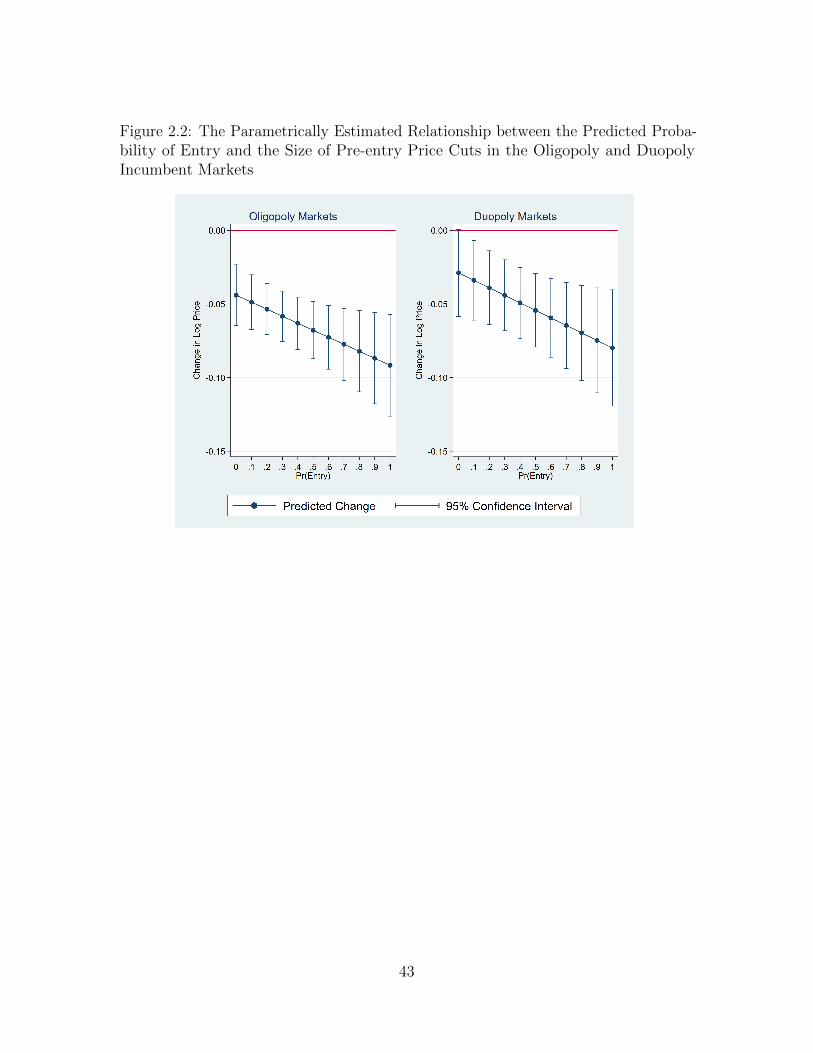
Figure 2.2: The Parametrically Estimated Relationship between the Predicted Proba-bility of Entry and the Size of Pre-entry Price Cuts in the Oligopoly and DuopolyIncumbent Markets
43
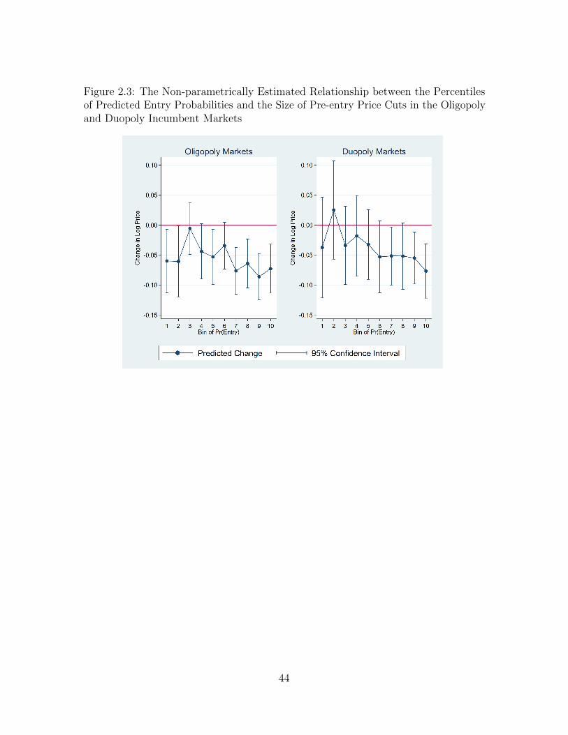
Figure 2.3: The Non-parametrically Estimated Relationship between the Percentilesof Predicted Entry Probabilities and the Size of Pre-entry Price Cuts in the Oligopolyand Duopoly Incumbent Markets
44
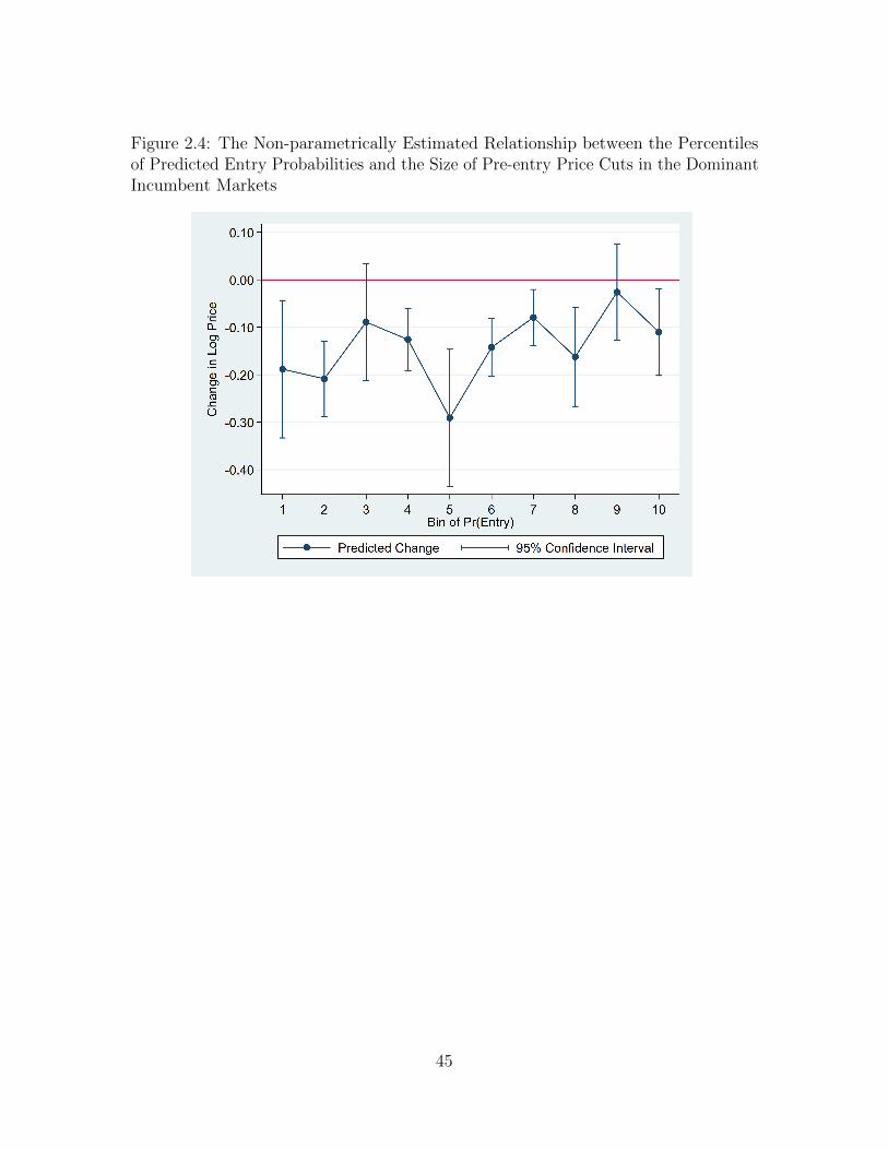
Figure 2.4: The Non-parametrically Estimated Relationship between the Percentilesof Predicted Entry Probabilities and the Size of Pre-entry Price Cuts in the DominantIncumbent Markets
45
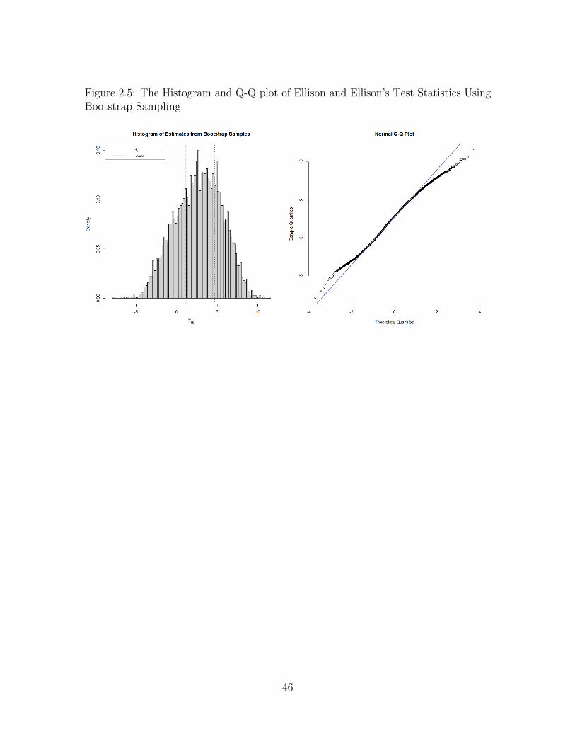
Figure 2.5: The Histogram and Q-Q plot of Ellison and Ellison’s Test Statistics UsingBootstrap Sampling
46
Chapter 3
The Effect of Entry Threat on
Incumbent Price Distribution:
Evidence from the Airline Industry
3.1 Introduction
Significant work in industrial economics has studied incumbent responses to the
threat of potential entry (even before actual entry occurs). As documented in Wilson
(1992), theoretical studies have analyzed various pre-entry responses in the context of
strategic entry deterrence. Incumbent firms can deter entry by signaling unprofitable
entry to potential entrants (Riley, 1980; Milgrom and Roberts, 1982a), which is
called limit pricing; predating a current entrant to threaten subsequent potential
entrants (Saloner, 1987; Milgrom and Roberts, 1982b); and establishing a preemptive
commitment through early investment (Eaton and Lipsey, 1979; Schmalensee, 1978;
Judd, 1985; Bonanno, 1987).
Earlier studies have generally focused on incumbent monopolists’ response
47
to entry threat, solely interpreting the motivation of such response as strategic
entry deterrence. However, those studies have paid less attention to oligopolistic
competition. Other than strategic entry deterrence, incumbent oligopolists may also
have an alternative motivation to respond to the appearance of a potential entrant.
With the possibility of tacitly colluding in oligopoly markets, more breakdowns in
tacit collusion occur as the likelihood of entry increases. Consequently, incumbent
oligopolists might want to decrease prices below their collusive level to prevent
deviation while the payoff of cheating becomes relatively attractive to them (Shin,
2021a).
This study empirically examines the underlying motivations of monopoly and
oligopoly incumbent responses to entry threat from Southwest Airlines. I rely on the
testable predictions in Shin (2021a) that differentiate two motivations: an attempt to
deter entry and a breakdown in tacit collusion. Intuitively speaking, if an incumbent
attempts to deter entry, pre-entry price cuts will be largest on routes where there is an
intermediate probability of entry since deterrence strategies are unlikely to be beneficial
on routes where entry is very unlikely or very likely. On the other hand, in the case
of breakdowns in tacit collusion, pre-entry price cuts will become monotonically larger
as the probability of entry increases since higher entry probabilities make collusion
harder to sustain.
As an extension of Shin (2021b), this paper employs incumbent carriers’ price
distribution (particularly percentiles of ticket fares) to test the motivation of pre-entry
responses. The basic idea is to compare how incumbents adjust their higher fares
(paid by business travelers) and their lower fares (paid by leisure travelers) in response
to a threat of entry. Business travelers are less price-elastic than leisure travelers so
that they are more likely to purchase higher fares.
In the context of strategic entry deterrence, incumbent carriers could signal
48
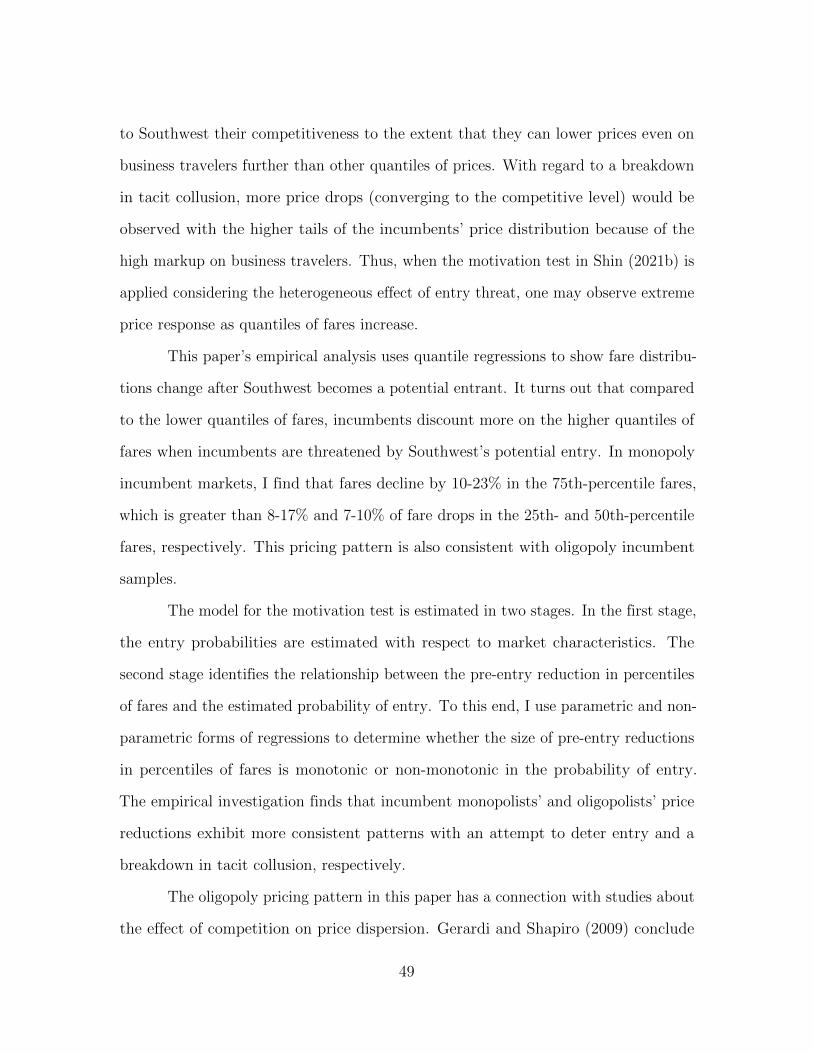
to Southwest their competitiveness to the extent that they can lower prices even on
business travelers further than other quantiles of prices. With regard to a breakdown
in tacit collusion, more price drops (converging to the competitive level) would be
observed with the higher tails of the incumbents’ price distribution because of the
high markup on business travelers. Thus, when the motivation test in Shin (2021b) is
applied considering the heterogeneous effect of entry threat, one may observe extreme
price response as quantiles of fares increase.
This paper’s empirical analysis uses quantile regressions to show fare distribu-
tions change after Southwest becomes a potential entrant. It turns out that compared
to the lower quantiles of fares, incumbents discount more on the higher quantiles of
fares when incumbents are threatened by Southwest’s potential entry. In monopoly
incumbent markets, I find that fares decline by 10-23% in the 75th-percentile fares,
which is greater than 8-17% and 7-10% of fare drops in the 25th- and 50th-percentile
fares, respectively. This pricing pattern is also consistent with oligopoly incumbent
samples.
The model for the motivation test is estimated in two stages. In the first stage,
the entry probabilities are estimated with respect to market characteristics. The
second stage identifies the relationship between the pre-entry reduction in percentiles
of fares and the estimated probability of entry. To this end, I use parametric and non-
parametric forms of regressions to determine whether the size of pre-entry reductions
in percentiles of fares is monotonic or non-monotonic in the probability of entry.
The empirical investigation finds that incumbent monopolists’ and oligopolists’ price
reductions exhibit more consistent patterns with an attempt to deter entry and a
breakdown in tacit collusion, respectively.
The oligopoly pricing pattern in this paper has a connection with studies about
the effect of competition on price dispersion. Gerardi and Shapiro (2009) conclude
49
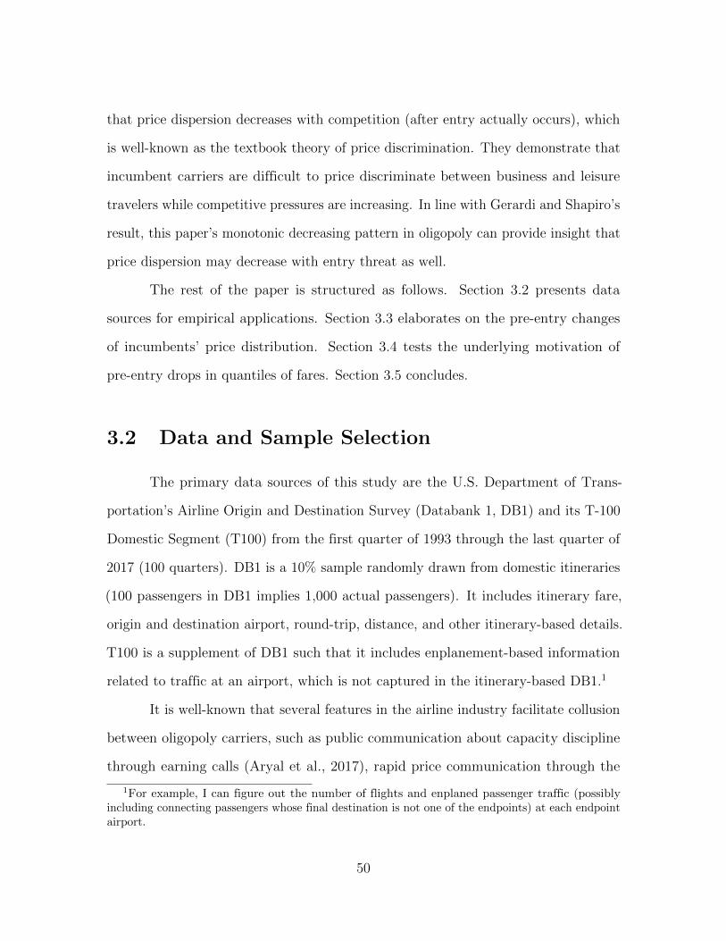
that price dispersion decreases with competition (after entry actually occurs), which
is well-known as the textbook theory of price discrimination. They demonstrate that
incumbent carriers are difficult to price discriminate between business and leisure
travelers while competitive pressures are increasing. In line with Gerardi and Shapiro’s
result, this paper’s monotonic decreasing pattern in oligopoly can provide insight that
price dispersion may decrease with entry threat as well.
The rest of the paper is structured as follows. Section 3.2 presents data
sources for empirical applications. Section 3.3 elaborates on the pre-entry changes
of incumbents’ price distribution. Section 3.4 tests the underlying motivation of
pre-entry drops in quantiles of fares. Section 3.5 concludes.
3.2 Data and Sample Selection
The primary data sources of this study are the U.S. Department of Trans-
portation’s Airline Origin and Destination Survey (Databank 1, DB1) and its T-100
Domestic Segment (T100) from the first quarter of 1993 through the last quarter of
2017 (100 quarters). DB1 is a 10% sample randomly drawn from domestic itineraries
(100 passengers in DB1 implies 1,000 actual passengers). It includes itinerary fare,
origin and destination airport, round-trip, distance, and other itinerary-based details.
T100 is a supplement of DB1 such that it includes enplanement-based information
related to traffic at an airport, which is not captured in the itinerary-based DB1.1
It is well-known that several features in the airline industry facilitate collusion
between oligopoly carriers, such as public communication about capacity discipline
through earning calls (Aryal et al., 2017), rapid price communication through the
1For example, I can figure out the number of flights and enplaned passenger traffic (possiblyincluding connecting passengers whose final destination is not one of the endpoints) at each endpointairport.
50
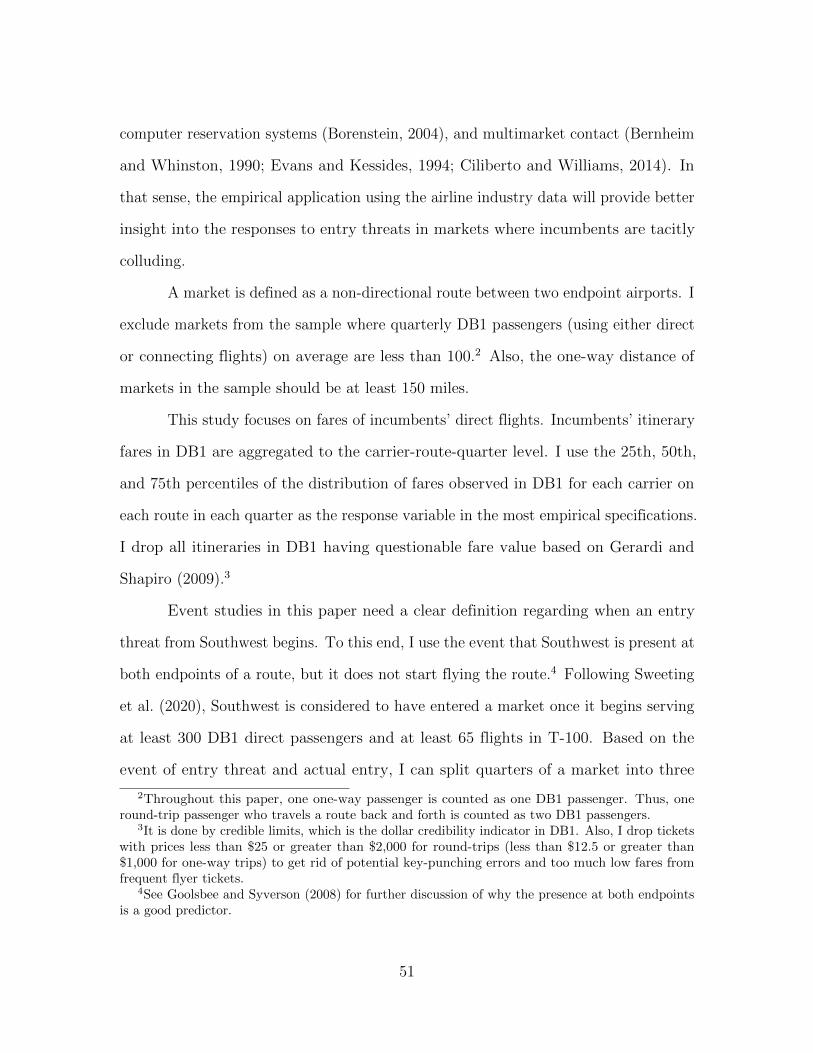
computer reservation systems (Borenstein, 2004), and multimarket contact (Bernheim
and Whinston, 1990; Evans and Kessides, 1994; Ciliberto and Williams, 2014). In
that sense, the empirical application using the airline industry data will provide better
insight into the responses to entry threats in markets where incumbents are tacitly
colluding.
A market is defined as a non-directional route between two endpoint airports. I
exclude markets from the sample where quarterly DB1 passengers (using either direct
or connecting flights) on average are less than 100.2 Also, the one-way distance of
markets in the sample should be at least 150 miles.
This study focuses on fares of incumbents’ direct flights. Incumbents’ itinerary
fares in DB1 are aggregated to the carrier-route-quarter level. I use the 25th, 50th,
and 75th percentiles of the distribution of fares observed in DB1 for each carrier on
each route in each quarter as the response variable in the most empirical specifications.
I drop all itineraries in DB1 having questionable fare value based on Gerardi and
Shapiro (2009).3
Event studies in this paper need a clear definition regarding when an entry
threat from Southwest begins. To this end, I use the event that Southwest is present at
both endpoints of a route, but it does not start flying the route.4 Following Sweeting
et al. (2020), Southwest is considered to have entered a market once it begins serving
at least 300 DB1 direct passengers and at least 65 flights in T-100. Based on the
event of entry threat and actual entry, I can split quarters of a market into three
2Throughout this paper, one one-way passenger is counted as one DB1 passenger. Thus, oneround-trip passenger who travels a route back and forth is counted as two DB1 passengers.
3It is done by credible limits, which is the dollar credibility indicator in DB1. Also, I drop ticketswith prices less than $25 or greater than $2,000 for round-trips (less than $12.5 or greater than$1,000 for one-way trips) to get rid of potential key-punching errors and too much low fares fromfrequent flyer tickets.
4See Goolsbee and Syverson (2008) for further discussion of why the presence at both endpointsis a good predictor.
51
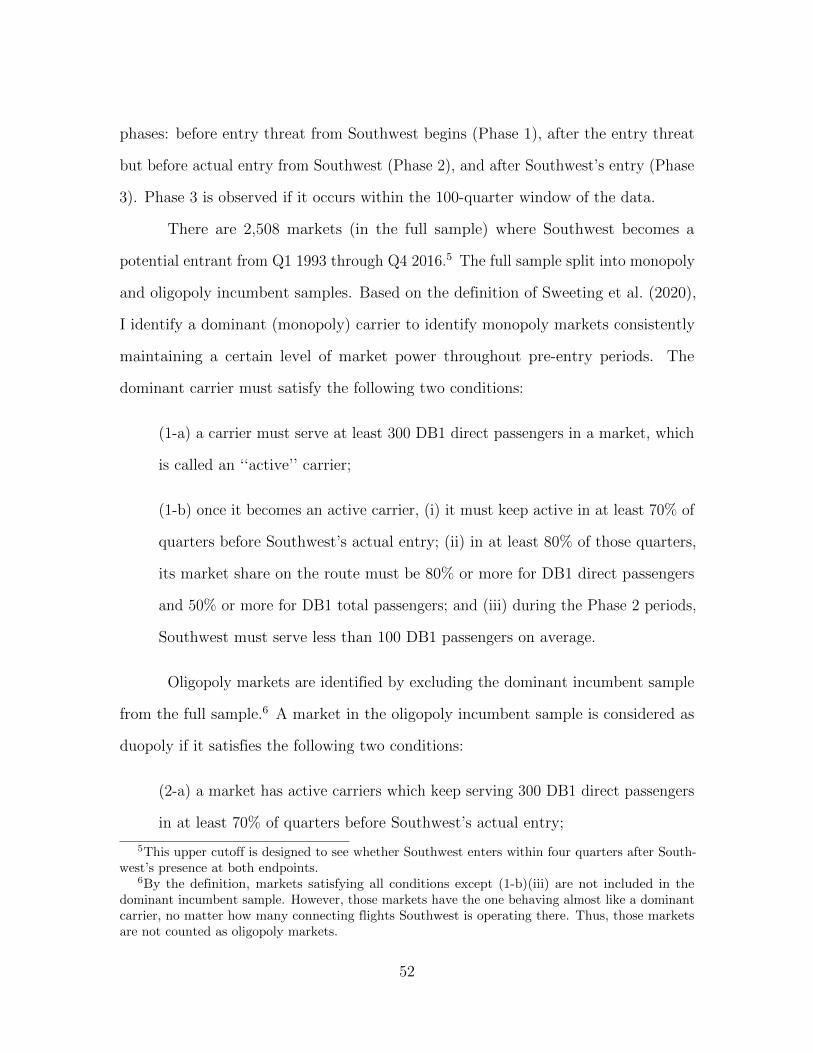
phases: before entry threat from Southwest begins (Phase 1), after the entry threat
but before actual entry from Southwest (Phase 2), and after Southwest’s entry (Phase
3). Phase 3 is observed if it occurs within the 100-quarter window of the data.
There are 2,508 markets (in the full sample) where Southwest becomes a
potential entrant from Q1 1993 through Q4 2016.5 The full sample split into monopoly
and oligopoly incumbent samples. Based on the definition of Sweeting et al. (2020),
I identify a dominant (monopoly) carrier to identify monopoly markets consistently
maintaining a certain level of market power throughout pre-entry periods. The
dominant carrier must satisfy the following two conditions:
(1-a) a carrier must serve at least 300 DB1 direct passengers in a market, which
is called an ‘‘active’’ carrier;
(1-b) once it becomes an active carrier, (i) it must keep active in at least 70% of
quarters before Southwest’s actual entry; (ii) in at least 80% of those quarters,
its market share on the route must be 80% or more for DB1 direct passengers
and 50% or more for DB1 total passengers; and (iii) during the Phase 2 periods,
Southwest must serve less than 100 DB1 passengers on average.
Oligopoly markets are identified by excluding the dominant incumbent sample
from the full sample.6 A market in the oligopoly incumbent sample is considered as
duopoly if it satisfies the following two conditions:
(2-a) a market has active carriers which keep serving 300 DB1 direct passengers
in at least 70% of quarters before Southwest’s actual entry;
5This upper cutoff is designed to see whether Southwest enters within four quarters after South-west’s presence at both endpoints.
6By the definition, markets satisfying all conditions except (1-b)(iii) are not included in thedominant incumbent sample. However, those markets have the one behaving almost like a dominantcarrier, no matter how many connecting flights Southwest is operating there. Thus, those marketsare not counted as oligopoly markets.
52
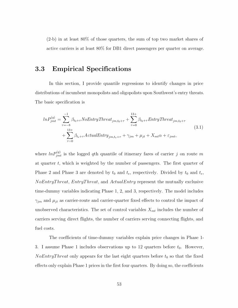
(2-b) in at least 80% of those quarters, the sum of top two market shares of
active carriers is at least 80% for DB1 direct passengers per quarter on average.
3.3 Empirical Specifications
In this section, I provide quantile regressions to identify changes in price
distributions of incumbent monopolists and oligopolists upon Southwest’s entry threats.
The basic specification is
lnP(q)jmt =
−1∑τ=−8
βt0+τNoEntryThreat jm,t0+τ +13+∑τ=0
βt0+τEntryThreat jm,t0+τ
+13+∑τ=0
βte+τActualEntry jm,te+τ + γjm + µjt +Xmtα + εjmt,
(3.1)
where lnP(q)jmt is the logged qth quantile of itinerary fares of carrier j on route m
at quarter t, which is weighted by the number of passengers. The first quarter of
Phase 2 and Phase 3 are denoted by t0 and te, respectively. Divided by t0 and te,
NoEntryThreat, EntryThreat, and ActualEntry represent the mutually exclusive
time-dummy variables indicating Phase 1, 2, and 3, respectively. The model includes
γjm and µjt as carrier-route and carrier-quarter fixed effects to control the impact of
unobserved characteristics. The set of control variables Xmt includes the number of
carriers serving direct flights, the number of carriers serving connecting flights, and
fuel costs.
The coefficients of time-dummy variables explain price changes in Phase 1-
3. I assume Phase 1 includes observations up to 12 quarters before t0. However,
NoEntryThreat only appears for the last eight quarters before t0 so that the fixed
effects only explain Phase 1 prices in the first four quarters. By doing so, the coefficients
53
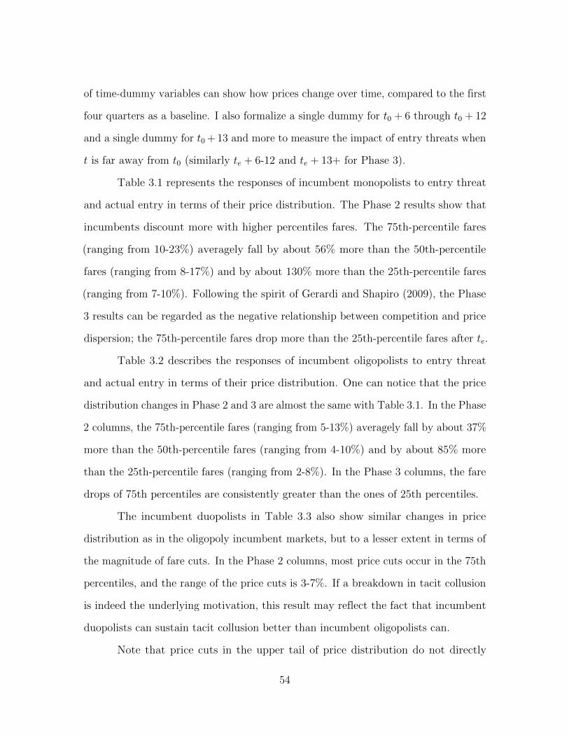
of time-dummy variables can show how prices change over time, compared to the first
four quarters as a baseline. I also formalize a single dummy for t0 + 6 through t0 + 12
and a single dummy for t0 + 13 and more to measure the impact of entry threats when
t is far away from t0 (similarly te + 6-12 and te + 13+ for Phase 3).
Table 3.1 represents the responses of incumbent monopolists to entry threat
and actual entry in terms of their price distribution. The Phase 2 results show that
incumbents discount more with higher percentiles fares. The 75th-percentile fares
(ranging from 10-23%) averagely fall by about 56% more than the 50th-percentile
fares (ranging from 8-17%) and by about 130% more than the 25th-percentile fares
(ranging from 7-10%). Following the spirit of Gerardi and Shapiro (2009), the Phase
3 results can be regarded as the negative relationship between competition and price
dispersion; the 75th-percentile fares drop more than the 25th-percentile fares after te.
Table 3.2 describes the responses of incumbent oligopolists to entry threat
and actual entry in terms of their price distribution. One can notice that the price
distribution changes in Phase 2 and 3 are almost the same with Table 3.1. In the Phase
2 columns, the 75th-percentile fares (ranging from 5-13%) averagely fall by about 37%
more than the 50th-percentile fares (ranging from 4-10%) and by about 85% more
than the 25th-percentile fares (ranging from 2-8%). In the Phase 3 columns, the fare
drops of 75th percentiles are consistently greater than the ones of 25th percentiles.
The incumbent duopolists in Table 3.3 also show similar changes in price
distribution as in the oligopoly incumbent markets, but to a lesser extent in terms of
the magnitude of fare cuts. In the Phase 2 columns, most price cuts occur in the 75th
percentiles, and the range of the price cuts is 3-7%. If a breakdown in tacit collusion
is indeed the underlying motivation, this result may reflect the fact that incumbent
duopolists can sustain tacit collusion better than incumbent oligopolists can.
Note that price cuts in the upper tail of price distribution do not directly
54
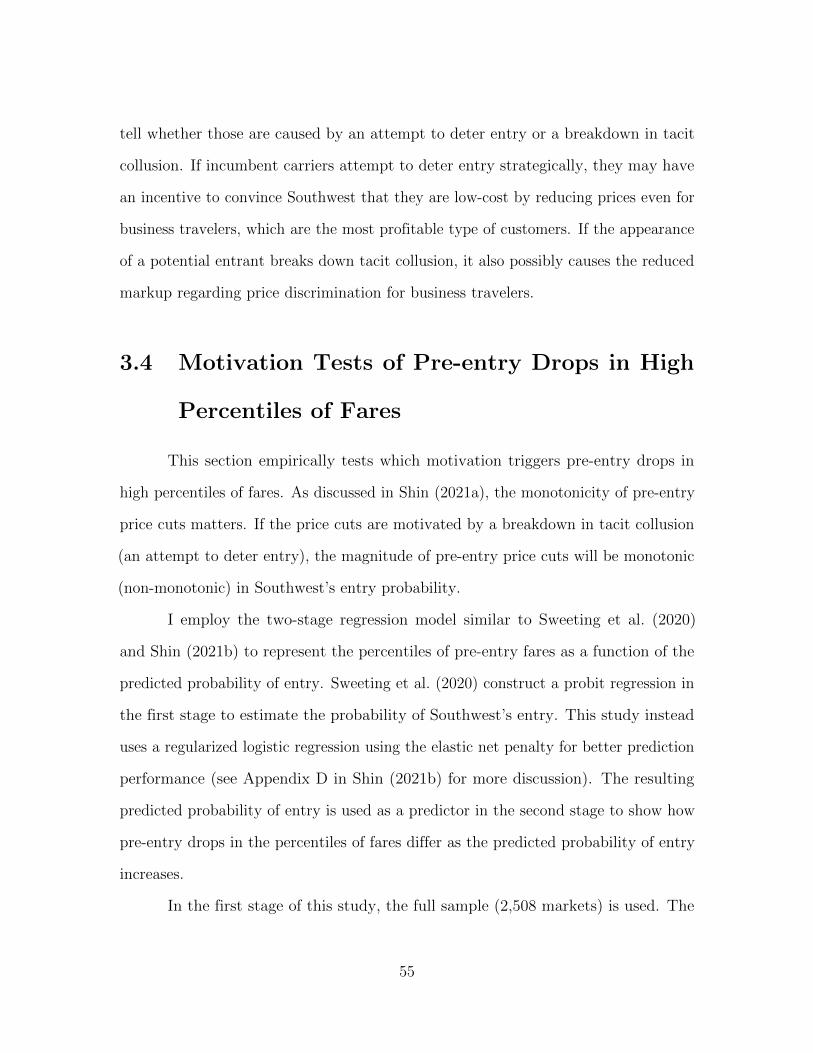
tell whether those are caused by an attempt to deter entry or a breakdown in tacit
collusion. If incumbent carriers attempt to deter entry strategically, they may have
an incentive to convince Southwest that they are low-cost by reducing prices even for
business travelers, which are the most profitable type of customers. If the appearance
of a potential entrant breaks down tacit collusion, it also possibly causes the reduced
markup regarding price discrimination for business travelers.
3.4 Motivation Tests of Pre-entry Drops in High
Percentiles of Fares
This section empirically tests which motivation triggers pre-entry drops in
high percentiles of fares. As discussed in Shin (2021a), the monotonicity of pre-entry
price cuts matters. If the price cuts are motivated by a breakdown in tacit collusion
(an attempt to deter entry), the magnitude of pre-entry price cuts will be monotonic
(non-monotonic) in Southwest’s entry probability.
I employ the two-stage regression model similar to Sweeting et al. (2020)
and Shin (2021b) to represent the percentiles of pre-entry fares as a function of the
predicted probability of entry. Sweeting et al. (2020) construct a probit regression in
the first stage to estimate the probability of Southwest’s entry. This study instead
uses a regularized logistic regression using the elastic net penalty for better prediction
performance (see Appendix D in Shin (2021b) for more discussion). The resulting
predicted probability of entry is used as a predictor in the second stage to show how
pre-entry drops in the percentiles of fares differ as the predicted probability of entry
increases.
In the first stage of this study, the full sample (2,508 markets) is used. The
55
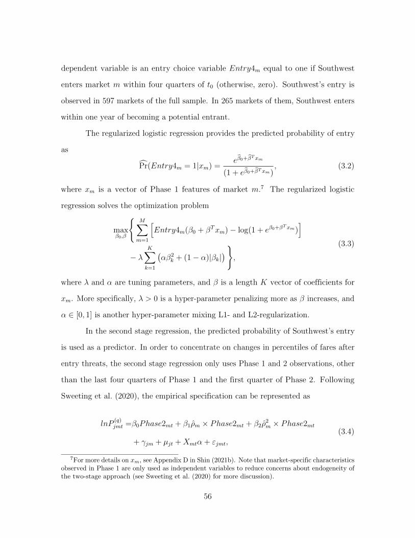
dependent variable is an entry choice variable Entry4m equal to one if Southwest
enters market m within four quarters of t0 (otherwise, zero). Southwest’s entry is
observed in 597 markets of the full sample. In 265 markets of them, Southwest enters
within one year of becoming a potential entrant.
The regularized logistic regression provides the predicted probability of entry
as
Pr(Entry4m = 1|xm) =eβ0+β
T xm
(1 + eβ0+βT xm), (3.2)
where xm is a vector of Phase 1 features of market m.7 The regularized logistic
regression solves the optimization problem
(3.3)
maxβ0,β
{M∑m=1
[Entry4m(β0 + βTxm)− log(1 + eβ0+β
T xm)]
− λK∑k=1
(αβ2
k + (1− α)|βk|)}
,
where λ and α are tuning parameters, and β is a length K vector of coefficients for
xm. More specifically, λ > 0 is a hyper-parameter penalizing more as β increases, and
α ∈ [0, 1] is another hyper-parameter mixing L1- and L2-regularization.
In the second stage regression, the predicted probability of Southwest’s entry
is used as a predictor. In order to concentrate on changes in percentiles of fares after
entry threats, the second stage regression only uses Phase 1 and 2 observations, other
than the last four quarters of Phase 1 and the first quarter of Phase 2. Following
Sweeting et al. (2020), the empirical specification can be represented as
lnP(q)jmt =β0Phase2mt + β1ρm × Phase2mt + β2ρ
2m × Phase2mt
+ γjm + µjt +Xmtα + εjmt,
(3.4)
7For more details on xm, see Appendix D in Shin (2021b). Note that market-specific characteristicsobserved in Phase 1 are only used as independent variables to reduce concerns about endogeneity ofthe two-stage approach (see Sweeting et al. (2020) for more discussion).
56
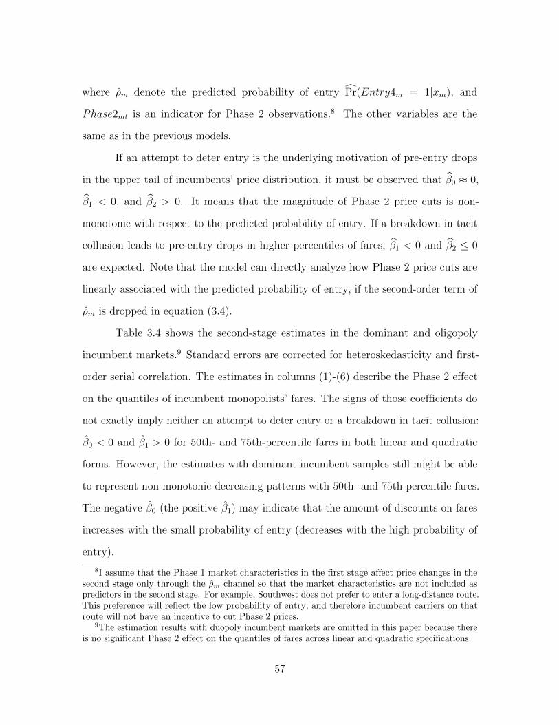
where ρm denote the predicted probability of entry Pr(Entry4m = 1|xm), and
Phase2mt is an indicator for Phase 2 observations.8 The other variables are the
same as in the previous models.
If an attempt to deter entry is the underlying motivation of pre-entry drops
in the upper tail of incumbents’ price distribution, it must be observed that β0 ≈ 0,
β1 < 0, and β2 > 0. It means that the magnitude of Phase 2 price cuts is non-
monotonic with respect to the predicted probability of entry. If a breakdown in tacit
collusion leads to pre-entry drops in higher percentiles of fares, β1 < 0 and β2 ≤ 0
are expected. Note that the model can directly analyze how Phase 2 price cuts are
linearly associated with the predicted probability of entry, if the second-order term of
ρm is dropped in equation (3.4).
Table 3.4 shows the second-stage estimates in the dominant and oligopoly
incumbent markets.9 Standard errors are corrected for heteroskedasticity and first-
order serial correlation. The estimates in columns (1)-(6) describe the Phase 2 effect
on the quantiles of incumbent monopolists’ fares. The signs of those coefficients do
not exactly imply neither an attempt to deter entry or a breakdown in tacit collusion:
β0 < 0 and β1 > 0 for 50th- and 75th-percentile fares in both linear and quadratic
forms. However, the estimates with dominant incumbent samples still might be able
to represent non-monotonic decreasing patterns with 50th- and 75th-percentile fares.
The negative β0 (the positive β1) may indicate that the amount of discounts on fares
increases with the small probability of entry (decreases with the high probability of
entry).
8I assume that the Phase 1 market characteristics in the first stage affect price changes in thesecond stage only through the ρm channel so that the market characteristics are not included aspredictors in the second stage. For example, Southwest does not prefer to enter a long-distance route.This preference will reflect the low probability of entry, and therefore incumbent carriers on thatroute will not have an incentive to cut Phase 2 prices.
9The estimation results with duopoly incumbent markets are omitted in this paper because thereis no significant Phase 2 effect on the quantiles of fares across linear and quadratic specifications.
57
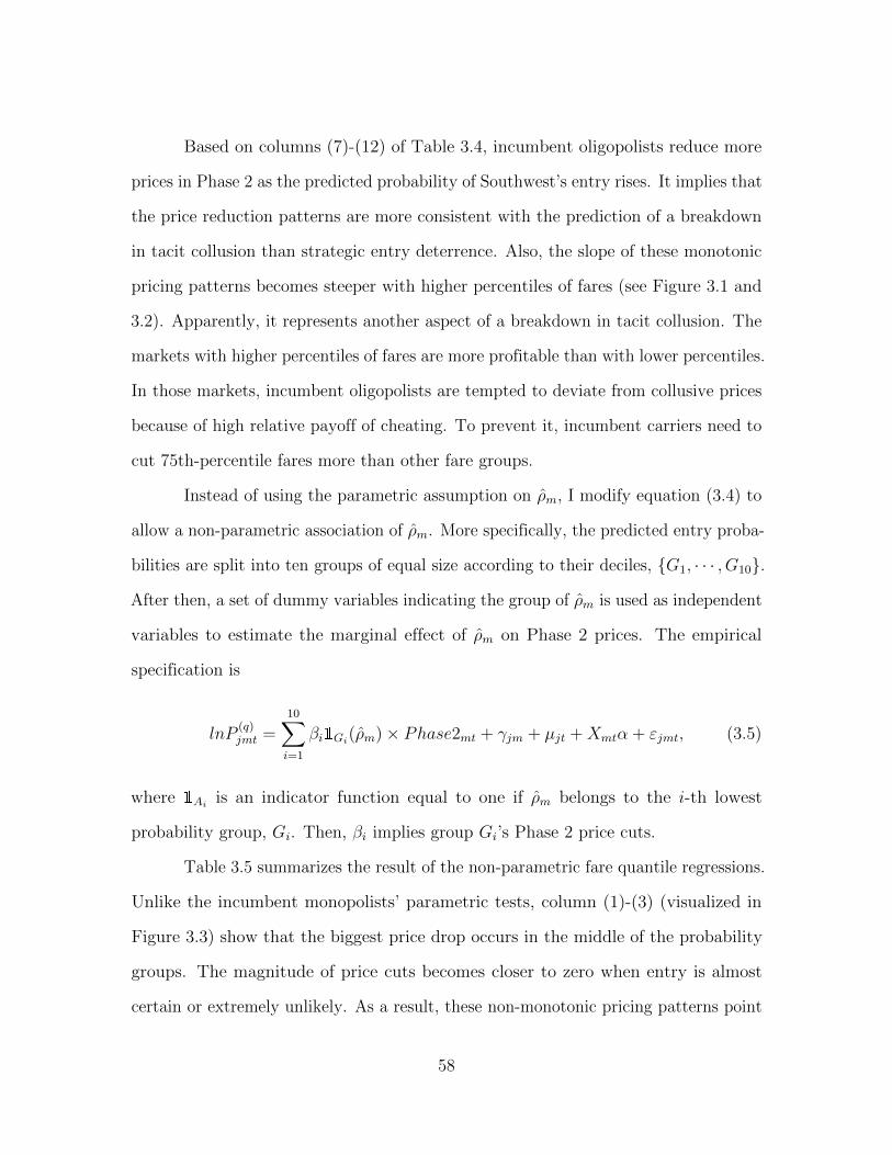
Based on columns (7)-(12) of Table 3.4, incumbent oligopolists reduce more
prices in Phase 2 as the predicted probability of Southwest’s entry rises. It implies that
the price reduction patterns are more consistent with the prediction of a breakdown
in tacit collusion than strategic entry deterrence. Also, the slope of these monotonic
pricing patterns becomes steeper with higher percentiles of fares (see Figure 3.1 and
3.2). Apparently, it represents another aspect of a breakdown in tacit collusion. The
markets with higher percentiles of fares are more profitable than with lower percentiles.
In those markets, incumbent oligopolists are tempted to deviate from collusive prices
because of high relative payoff of cheating. To prevent it, incumbent carriers need to
cut 75th-percentile fares more than other fare groups.
Instead of using the parametric assumption on ρm, I modify equation (3.4) to
allow a non-parametric association of ρm. More specifically, the predicted entry proba-
bilities are split into ten groups of equal size according to their deciles, {G1, · · · , G10}.
After then, a set of dummy variables indicating the group of ρm is used as independent
variables to estimate the marginal effect of ρm on Phase 2 prices. The empirical
specification is
lnP(q)jmt =
10∑i=1
βi1Gi(ρm)× Phase2mt + γjm + µjt +Xmtα + εjmt, (3.5)
where 1Aiis an indicator function equal to one if ρm belongs to the i-th lowest
probability group, Gi. Then, βi implies group Gi’s Phase 2 price cuts.
Table 3.5 summarizes the result of the non-parametric fare quantile regressions.
Unlike the incumbent monopolists’ parametric tests, column (1)-(3) (visualized in
Figure 3.3) show that the biggest price drop occurs in the middle of the probability
groups. The magnitude of price cuts becomes closer to zero when entry is almost
certain or extremely unlikely. As a result, these non-monotonic pricing patterns point
58
out that the dominant incumbent carriers engage in limit pricing to deter Southwest’s
entry. More importantly, the result of 75th-percentile fares shows the deepest non-
monotonic decreasing pattern across the percentiles of fares. It means that incumbent
carriers could signal to Southwest that they have very low costs by lowering prices on
business travelers, the most profitable type of customer willing to pay relatively higher
fares. Overall, this extreme limit price could lower Southwest’s expected post-entry
profits and eventually discourage entry. Column (4)-(6) in Table 3.5 (visualized in
Figure 3.4) show the magnitude of Phase 2 price cuts in the oligopoly incumbent
markets is monotonic in the predicted probability of entry, which is consistent with
their parametric tests.
3.5 Conclusion
This study empirically investigates the underlying motivation of incumbent
reaction to the threat of potential entry in terms of price distribution. I use the testable
predictions in Shin (2021a) to examine whether the changes in price distribution are
driven by a breakdown in tacit collusion or an attempt to deter entry. Using the
airline industry data and quantile regressions, the empirical model focuses on how
quantiles of ticket fares change after Southwest Airlines becomes a potential entrant
and how those changes are associated with the estimated probability of entry.
I employ a two-stage model to test the relationship between the price drops
and the likelihood of entry. In the first stage, the entry probabilities are estimated
with a regularized logistic regression, which shows better prediction performances.
In the second stage, I construct parametric and non-parametric quantile regressions
using the predicted probability of entry as a predictor variable. The empirical models
determine whether the reduction patterns of pre-entry prices are consistent with the
59
prediction of breakdowns in tacit collusion or strategic entry deterrence.
The two-stage motivation tests indicate that the magnitude of pre-entry price
reductions in dominant (oligopoly) incumbent markets is non-monotonic (monotonic)
in the predicted probability of Southwest’s entry. It implies that the underlying
motivation of the dominant (oligopoly) incumbent responses is more consistent with
the prediction of an attempt to deter entry (a breakdown in tacit collusion). The
analysis in Shin (2021b) does not find remarkable evidence that incumbent monopolists
use limit pricing to deter entry, which is the main result in Sweeting et al. (2020).
However, this paper’s empirical tests provide consistent evidence that strategic entry
deterrence is the underlying motivation in the dominant incumbent markets.
60
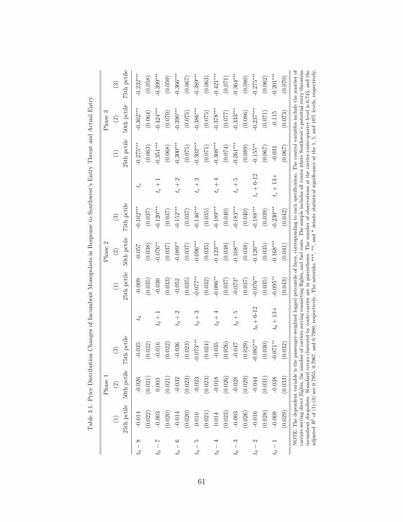
Tab
le3.
1:P
rice
Dis
trib
uti
onC
han
ges
ofIn
cum
ben
tM
onop
olis
tsin
Res
pon
seto
Sou
thw
est’
sE
ntr
yT
hre
atan
dA
ctual
Entr
y
Phas
e1
Phas
e2
Phas
e3
(1)
(2)
(3)
(1)
(2)
(3)
(1)
(2)
(3)
25th
pct
ile
50th
pct
ile
75th
pct
ile
25th
pct
ile
50th
pct
ile
75th
pct
ile
25th
pct
ile
50th
pct
ile
75th
pct
ile
t 0−
8-0
.014
-0.0
26-0
.035
t 0-0
.009
-0.0
57-0
.102∗∗∗
t e-0
.275∗∗∗
-0.3
02∗∗∗
-0.2
32∗∗∗
(0.0
22)
(0.0
21)
(0.0
22)
(0.0
35)
(0.0
38)
(0.0
37)
(0.0
63)
(0.0
64)
(0.0
58)
t 0−
7-0
.003
0.00
3-0
.016
t 0+
1-0
.030
-0.0
76∗∗
-0.1
20∗∗∗
t e+
1-0
.351∗∗∗
-0.4
24∗∗∗
-0.3
99∗∗∗
(0.0
20)
(0.0
21)
(0.0
22)
(0.0
33)
(0.0
37)
(0.0
37)
(0.0
68)
(0.0
70)
(0.0
59)
t 0−
6-0
.014
-0.0
32-0
.036
t 0+
2-0
.052
-0.0
89∗∗
-0.1
52∗∗∗
t e+
2-0
.300∗∗∗
-0.3
90∗∗∗
-0.3
66∗∗∗
(0.0
20)
(0.0
23)
(0.0
23)
(0.0
35)
(0.0
37)
(0.0
37)
(0.0
75)
(0.0
75)
(0.0
67)
t 0−
50.
010
-0.0
23-0
.073∗∗∗
t 0+
3-0
.077∗∗
-0.0
96∗∗∗
-0.1
46∗∗∗
t e+
3-0
.302∗∗∗
-0.3
86∗∗∗
-0.3
89∗∗∗
(0.0
21)
(0.0
23)
(0.0
24)
(0.0
32)
(0.0
35)
(0.0
35)
(0.0
71)
(0.0
75)
(0.0
63)
t 0−
40.
014
-0.0
18-0
.035
t 0+
4-0
.086∗∗
-0.1
23∗∗∗
-0.1
89∗∗∗
t e+
4-0
.308∗∗∗
-0.3
78∗∗∗
-0.4
21∗∗∗
(0.0
23)
(0.0
26)
(0.0
26)
(0.0
37)
(0.0
38)
(0.0
40)
(0.0
74)
(0.0
77)
(0.0
71)
t 0−
3-0
.003
-0.0
28-0
.047
t 0+
5-0
.073∗
-0.1
08∗∗∗
-0.1
83∗∗∗
t e+
5-0
.261∗∗∗
-0.3
33∗∗∗
-0.3
64∗∗∗
(0.0
26)
(0.0
29)
(0.0
29)
(0.0
37)
(0.0
38)
(0.0
40)
(0.0
89)
(0.0
86)
(0.0
80)
t 0−
2-0
.016
-0.0
44-0
.085∗∗∗
t 0+
6-12
-0.0
76∗∗
-0.1
26∗∗∗
-0.1
88∗∗∗
t e+
6-12
-0.1
55∗∗
-0.2
37∗∗∗
-0.2
75∗∗∗
(0.0
28)
(0.0
31)
(0.0
30)
(0.0
35)
(0.0
35)
(0.0
39)
(0.0
67)
(0.0
71)
(0.0
62)
t 0−
1-0
.008
-0.0
38-0
.071∗∗
t 0+
13+
-0.0
95∗∗
-0.1
68∗∗∗
-0.2
30∗∗∗
t e+
13+
-0.0
31-0
.115
-0.2
01∗∗∗
(0.0
29)
(0.0
33)
(0.0
32)
(0.0
43)
(0.0
41)
(0.0
42)
(0.0
67)
(0.0
73)
(0.0
70)
NOTE:Thedep
enden
tvariable
isthepassen
ger-w
eightedlogged
percentile
offares,
correspondingto
each
specification.Thecontrolvariablesincludethenumber
of
carriers
servingdirectflights,thenumber
ofcarriers
servingconnectingflights,an
dfuel
costs.
Thesample
includes
allrouteswhereSou
thwest’spotential
entrythreatens
incumbentduopolists.
Standard
errors
clustered
byroute-carrierare
inparentheses.Thenumber
ofobservationsatthecarrier-route-quarter
level
is6,745,andthe
adjusted
R2of
(1)-(3)are0.79
55,0.796
7,an
d0.79
80,respectively.Theasterisks**
*,**
,and*den
ote
statisticalsignifican
ceatthe1,5,
and10
%levels,
respectively.
61
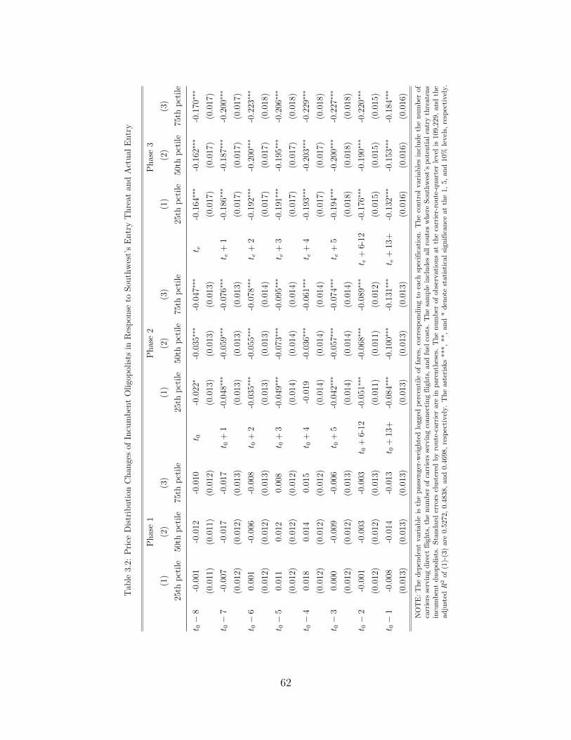
Tab
le3.
2:P
rice
Dis
trib
uti
onC
han
ges
ofIn
cum
ben
tO
ligo
pol
ists
inR
espon
seto
Sou
thw
est’
sE
ntr
yT
hre
atan
dA
ctual
Entr
y
Phas
e1
Phas
e2
Phas
e3
(1)
(2)
(3)
(1)
(2)
(3)
(1)
(2)
(3)
25th
pct
ile
50th
pct
ile
75th
pct
ile
25th
pct
ile
50th
pct
ile
75th
pct
ile
25th
pct
ile
50th
pct
ile
75th
pct
ile
t 0−
8-0
.001
-0.0
12-0
.010
t 0-0
.022∗
-0.0
35∗∗∗
-0.0
47∗∗∗
t e-0
.164∗∗∗
-0.1
62∗∗∗
-0.1
70∗∗∗
(0.0
11)
(0.0
11)
(0.0
12)
(0.0
13)
(0.0
13)
(0.0
13)
(0.0
17)
(0.0
17)
(0.0
17)
t 0−
7-0
.007
-0.0
17-0
.017
t 0+
1-0
.048∗∗∗
-0.0
59∗∗∗
-0.0
76∗∗∗
t e+
1-0
.186∗∗∗
-0.1
87∗∗∗
-0.2
00∗∗∗
(0.0
12)
(0.0
12)
(0.0
13)
(0.0
13)
(0.0
13)
(0.0
13)
(0.0
17)
(0.0
17)
(0.0
17)
t 0−
60.
001
-0.0
06-0
.008
t 0+
2-0
.035∗∗∗
-0.0
55∗∗∗
-0.0
78∗∗∗
t e+
2-0
.192∗∗∗
-0.2
00∗∗∗
-0.2
23∗∗∗
(0.0
12)
(0.0
12)
(0.0
13)
(0.0
13)
(0.0
13)
(0.0
14)
(0.0
17)
(0.0
17)
(0.0
18)
t 0−
50.
011
0.01
20.
008
t 0+
3-0
.049∗∗∗
-0.0
73∗∗∗
-0.0
95∗∗∗
t e+
3-0
.191∗∗∗
-0.1
95∗∗∗
-0.2
06∗∗∗
(0.0
12)
(0.0
12)
(0.0
12)
(0.0
14)
(0.0
14)
(0.0
14)
(0.0
17)
(0.0
17)
(0.0
18)
t 0−
40.
018
0.01
40.
015
t 0+
4-0
.019
-0.0
36∗∗∗
-0.0
61∗∗∗
t e+
4-0
.193∗∗∗
-0.2
03∗∗∗
-0.2
29∗∗∗
(0.0
12)
(0.0
12)
(0.0
12)
(0.0
14)
(0.0
14)
(0.0
14)
(0.0
17)
(0.0
17)
(0.0
18)
t 0−
30.
000
-0.0
09-0
.006
t 0+
5-0
.042∗∗∗
-0.0
57∗∗∗
-0.0
74∗∗∗
t e+
5-0
.194∗∗∗
-0.2
00∗∗∗
-0.2
27∗∗∗
(0.0
12)
(0.0
12)
(0.0
13)
(0.0
14)
(0.0
14)
(0.0
14)
(0.0
18)
(0.0
18)
(0.0
18)
t 0−
2-0
.001
-0.0
03-0
.003
t 0+
6-12
-0.0
51∗∗∗
-0.0
68∗∗∗
-0.0
89∗∗∗
t e+
6-12
-0.1
76∗∗∗
-0.1
90∗∗∗
-0.2
20∗∗∗
(0.0
12)
(0.0
12)
(0.0
13)
(0.0
11)
(0.0
11)
(0.0
12)
(0.0
15)
(0.0
15)
(0.0
15)
t 0−
1-0
.008
-0.0
14-0
.013
t 0+
13+
-0.0
84∗∗∗
-0.1
00∗∗∗
-0.1
31∗∗∗
t e+
13+
-0.1
32∗∗∗
-0.1
53∗∗∗
-0.1
84∗∗∗
(0.0
13)
(0.0
13)
(0.0
13)
(0.0
13)
(0.0
13)
(0.0
13)
(0.0
16)
(0.0
16)
(0.0
16)
NOTE:Thedep
enden
tvariable
isthepassen
ger-w
eightedlogged
percentile
offares,
correspondingto
each
specification.Thecontrolvariablesincludethenumber
of
carriers
servingdirectflights,thenumber
ofcarriers
servingconnectingflights,an
dfuel
costs.
Thesample
includes
allrouteswhereSou
thwest’spotential
entrythreatens
incu
mben
tduopolists.
Standarderrors
clustered
byroute-carrier
are
inparen
theses.Thenumber
ofobservation
satthecarrier-route-quarterlevel
is10
9,229
,andthe
adjusted
R2of
(1)-(3)are0.527
2,0.48
38,an
d0.469
8,respectively.Theasterisks**
*,**,
and*den
otestatistical
significan
ceatthe1,5,
and10
%levels,
respectively.
62
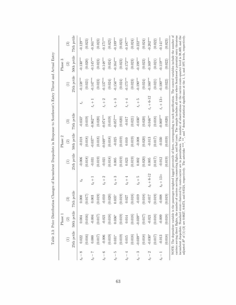
Tab
le3.
3:P
rice
Dis
trib
uti
onC
han
ges
ofIn
cum
ben
tD
uop
olis
tsin
Res
pon
seto
Sou
thw
est’
sE
ntr
yT
hre
atan
dA
ctual
Entr
y
Phas
e1
Phas
e2
Phas
e3
(1)
(2)
(3)
(1)
(2)
(3)
(1)
(2)
(3)
25th
pct
ile
50th
pct
ile
75th
pct
ile
25th
pct
ile
50th
pct
ile
75th
pct
ile
25th
pct
ile
50th
pct
ile
75th
pct
ile
t 0−
80.
022
0.00
40.
000
t 0-0
.006
-0.0
18-0
.033∗
t e-0
.138∗∗∗
-0.1
30∗∗∗
-0.1
29∗∗∗
(0.0
16)
(0.0
16)
(0.0
17)
(0.0
18)
(0.0
18)
(0.0
19)
(0.0
21)
(0.0
20)
(0.0
23)
t 0−
70.
000
-0.0
040.
003
t 0+
1-0
.031
-0.0
37∗∗
-0.0
62∗∗∗
t e+
1-0
.147∗∗∗
-0.1
45∗∗∗
-0.1
61∗∗∗
(0.0
17)
(0.0
17)
(0.0
19)
(0.0
19)
(0.0
18)
(0.0
20)
(0.0
23)
(0.0
23)
(0.0
23)
t 0−
6-0
.006
-0.0
21-0
.010
t 0+
2-0
.021
-0.0
49∗∗∗
-0.0
74∗∗∗
t e+
2-0
.137∗∗∗
-0.1
48∗∗∗
-0.1
71∗∗∗
(0.0
19)
(0.0
18)
(0.0
20)
(0.0
18)
(0.0
18)
(0.0
19)
(0.0
24)
(0.0
24)
(0.0
25)
t 0−
50.
031∗
0.03
6∗0.
035∗
t 0+
30.
005
-0.0
25-0
.057∗∗∗
t e+
3-0
.156∗∗∗
-0.1
64∗∗∗
-0.1
89∗∗∗
(0.0
19)
(0.0
19)
(0.0
19)
(0.0
19)
(0.0
19)
(0.0
20)
(0.0
24)
(0.0
23)
(0.0
23)
t 0−
40.
015
0.01
40.
027
t 0+
40.
023
0.01
0-0
.017
t e+
4-0
.175∗∗∗
-0.1
72∗∗∗
-0.1
87∗∗∗
(0.0
18)
(0.0
18)
(0.0
18)
(0.0
19)
(0.0
19)
(0.0
21)
(0.0
23)
(0.0
23)
(0.0
24)
t 0−
3-0
.039∗∗
-0.0
39∗∗
-0.0
19t 0
+5
0.00
2-0
.008
-0.0
36∗
t e+
5-0
.190∗∗∗
-0.1
98∗∗∗
-0.2
22∗∗∗
(0.0
18)
(0.0
17)
(0.0
18)
(0.0
20)
(0.0
20)
(0.0
20)
(0.0
24)
(0.0
23)
(0.0
24)
t 0−
2-0
.030∗
-0.0
21-0
.017
t 0+
6-12
0.00
5-0
.013
-0.0
46∗∗
t e+
6-12
-0.1
60∗∗∗
-0.1
69∗∗∗
-0.2
02∗∗∗
(0.0
17)
(0.0
18)
(0.0
19)
(0.0
17)
(0.0
17)
(0.0
18)
(0.0
21)
(0.0
21)
(0.0
22)
t 0−
1-0
.013
-0.0
09-0
.008
t 0+
13+
-0.0
12-0
.030
-0.0
69∗∗∗
t e+
13+
-0.1
00∗∗∗
-0.1
19∗∗∗
-0.1
41∗∗∗
(0.0
18)
(0.0
18)
(0.0
19)
(0.0
19)
(0.0
19)
(0.0
20)
(0.0
22)
(0.0
22)
(0.0
23)
NOTE:Thedep
enden
tvariable
isthepassen
ger-w
eightedlogged
percentile
offares,
correspondingto
each
specification.Thecontrolvariablesincludethenumber
of
carriers
servingdirectflights,thenumber
ofcarriers
servingconnectingflights,an
dfuel
costs.
Thesample
includes
allrouteswhereSou
thwest’spotential
entrythreatens
incumbentduopolists.
Standard
errors
clustered
byroute-carrierare
inparentheses.Thenumber
ofobservationsatthecarrier-route-quarter
level
is38,469,andthe
adjusted
R2of
(1)-(3)are0.662
7,0.64
73,an
d0.652
4,respectively.Theasterisks**
*,**,
and*den
otestatistical
significan
ceatthe1,5,
and10
%levels,
respectively.
63
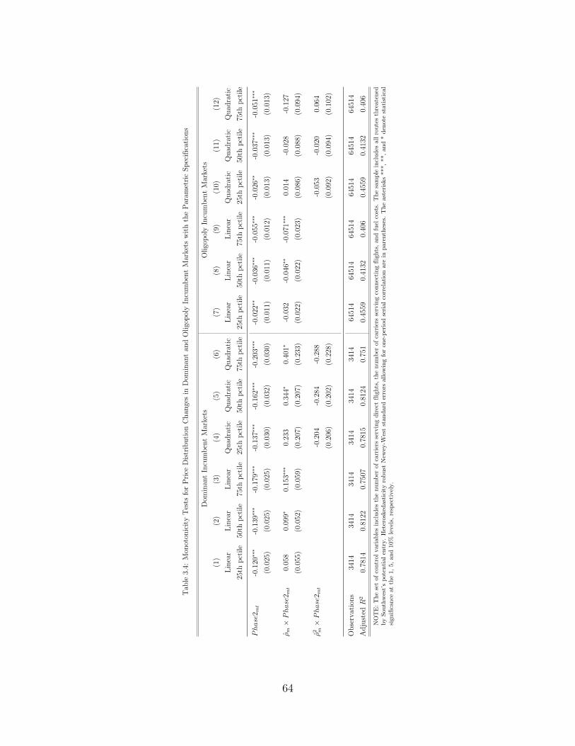
Tab
le3.
4:M
onot
onic
ity
Tes
tsfo
rP
rice
Dis
trib
uti
onC
han
ges
inD
omin
ant
and
Oligo
pol
yIn
cum
ben
tM
arket
sw
ith
the
Par
amet
ric
Spec
ific
atio
ns
Dom
inan
tIn
cum
ben
tM
arket
sO
ligo
pol
yIn
cum
ben
tM
arket
s
(1)
(2)
(3)
(4)
(5)
(6)
(7)
(8)
(9)
(10)
(11)
(12)
Lin
ear
Lin
ear
Lin
ear
Quad
rati
cQ
uad
rati
cQ
uad
rati
cL
inea
rL
inea
rL
inea
rQ
uad
rati
cQ
uad
rati
cQ
uad
rati
c
25th
pct
ile
50th
pct
ile
75th
pct
ile
25th
pct
ile
50th
pct
ile
75th
pct
ile
25th
pct
ile
50th
pct
ile
75th
pct
ile
25th
pct
ile
50th
pct
ile
75th
pct
ile
Phase
2 mt
-0.1
20∗∗∗
-0.1
39∗∗∗
-0.1
79∗∗∗
-0.1
37∗∗∗
-0.1
62∗∗∗
-0.2
03∗∗∗
-0.0
22∗∗
-0.0
36∗∗∗
-0.0
55∗∗∗
-0.0
26∗∗
-0.0
37∗∗∗
-0.0
51∗∗∗
(0.0
25)
(0.0
25)
(0.0
25)
(0.0
30)
(0.0
32)
(0.0
30)
(0.0
11)
(0.0
11)
(0.0
12)
(0.0
13)
(0.0
13)
(0.0
13)
ρm×Phase
2 mt
0.05
80.
099∗
0.15
3∗∗∗
0.23
30.
344∗
0.40
1∗-0
.032
-0.0
46∗∗
-0.0
71∗∗∗
0.01
4-0
.028
-0.1
27
(0.0
55)
(0.0
52)
(0.0
59)
(0.2
07)
(0.2
07)
(0.2
33)
(0.0
22)
(0.0
22)
(0.0
23)
(0.0
86)
(0.0
88)
(0.0
94)
ρ2 m×Phase
2 mt
-0.2
04-0
.284
-0.2
88-0
.053
-0.0
200.
064
(0.2
06)
(0.2
02)
(0.2
28)
(0.0
92)
(0.0
94)
(0.1
02)
Obse
rvat
ions
3414
3414
3414
3414
3414
3414
6451
464
514
6451
464
514
6451
464
514
Adju
sted
R2
0.78
140.
8122
0.75
070.
7815
0.81
240.
751
0.45
590.
4132
0.40
60.
4559
0.41
320.
406
NOTE:Thesetofcontrolvariablesincludes
thenumber
ofcarriers
servingdirectflights,thenumber
ofcarriers
servingconnectingflights,andfuel
costs.
Thesample
includes
allroutesthreatened
bySouthwest’spotentialen
try.Heterosked
asticityrobust
New
ey-W
eststandard
errors
allowingforone-periodserialcorrelationare
inparentheses.Theasterisks***,**,and*den
ote
statistical
sign
ifican
ceat
the1,
5,an
d10
%levels,
respectively.
64
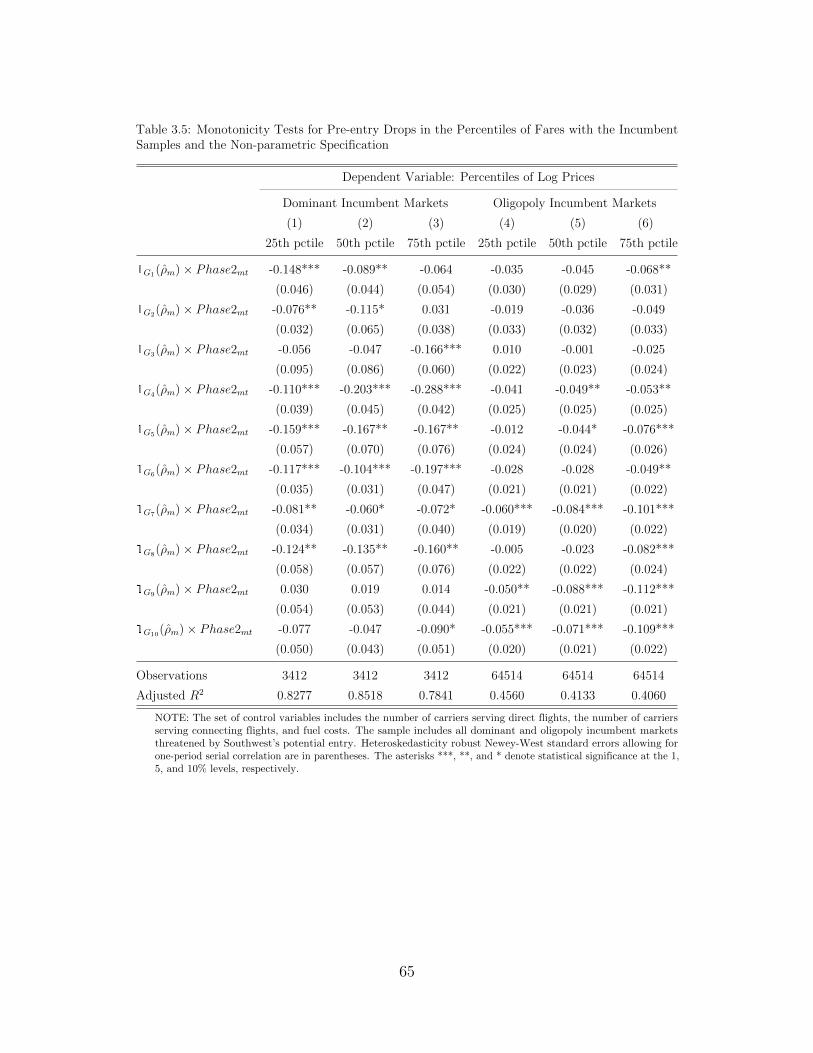
Table 3.5: Monotonicity Tests for Pre-entry Drops in the Percentiles of Fares with the IncumbentSamples and the Non-parametric Specification
Dependent Variable: Percentiles of Log Prices
Dominant Incumbent Markets Oligopoly Incumbent Markets
(1) (2) (3) (4) (5) (6)
25th pctile 50th pctile 75th pctile 25th pctile 50th pctile 75th pctile
1G1(ρm)× Phase2mt -0.148*** -0.089** -0.064 -0.035 -0.045 -0.068**
(0.046) (0.044) (0.054) (0.030) (0.029) (0.031)
1G2(ρm)× Phase2mt -0.076** -0.115* 0.031 -0.019 -0.036 -0.049
(0.032) (0.065) (0.038) (0.033) (0.032) (0.033)
1G3(ρm)× Phase2mt -0.056 -0.047 -0.166*** 0.010 -0.001 -0.025
(0.095) (0.086) (0.060) (0.022) (0.023) (0.024)
1G4(ρm)× Phase2mt -0.110*** -0.203*** -0.288*** -0.041 -0.049** -0.053**
(0.039) (0.045) (0.042) (0.025) (0.025) (0.025)
1G5(ρm)× Phase2mt -0.159*** -0.167** -0.167** -0.012 -0.044* -0.076***
(0.057) (0.070) (0.076) (0.024) (0.024) (0.026)
1G6(ρm)× Phase2mt -0.117*** -0.104*** -0.197*** -0.028 -0.028 -0.049**
(0.035) (0.031) (0.047) (0.021) (0.021) (0.022)
1G7(ρm)× Phase2mt -0.081** -0.060* -0.072* -0.060*** -0.084*** -0.101***
(0.034) (0.031) (0.040) (0.019) (0.020) (0.022)
1G8(ρm)× Phase2mt -0.124** -0.135** -0.160** -0.005 -0.023 -0.082***
(0.058) (0.057) (0.076) (0.022) (0.022) (0.024)
1G9(ρm)× Phase2mt 0.030 0.019 0.014 -0.050** -0.088*** -0.112***
(0.054) (0.053) (0.044) (0.021) (0.021) (0.021)
1G10(ρm)× Phase2mt -0.077 -0.047 -0.090* -0.055*** -0.071*** -0.109***
(0.050) (0.043) (0.051) (0.020) (0.021) (0.022)
Observations 3412 3412 3412 64514 64514 64514
Adjusted R2 0.8277 0.8518 0.7841 0.4560 0.4133 0.4060
NOTE: The set of control variables includes the number of carriers serving direct flights, the number of carriersserving connecting flights, and fuel costs. The sample includes all dominant and oligopoly incumbent marketsthreatened by Southwest’s potential entry. Heteroskedasticity robust Newey-West standard errors allowing forone-period serial correlation are in parentheses. The asterisks ***, **, and * denote statistical significance at the 1,5, and 10% levels, respectively.
65
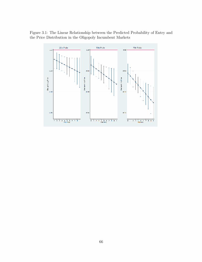
Figure 3.1: The Linear Relationship between the Predicted Probability of Entry andthe Price Distribution in the Oligopoly Incumbent Markets
66
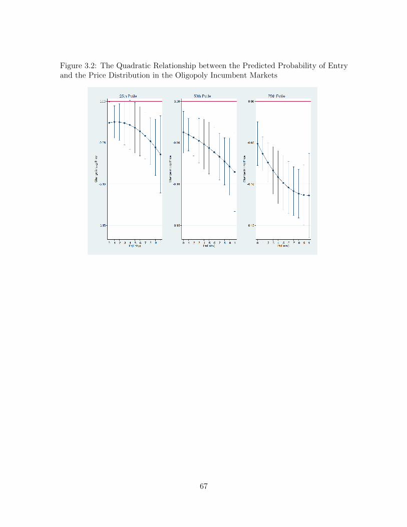
Figure 3.2: The Quadratic Relationship between the Predicted Probability of Entryand the Price Distribution in the Oligopoly Incumbent Markets
67
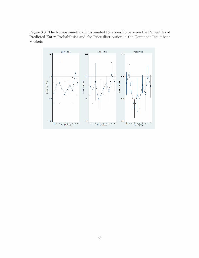
Figure 3.3: The Non-parametrically Estimated Relationship between the Percentiles ofPredicted Entry Probabilities and the Price distribution in the Dominant IncumbentMarkets
68
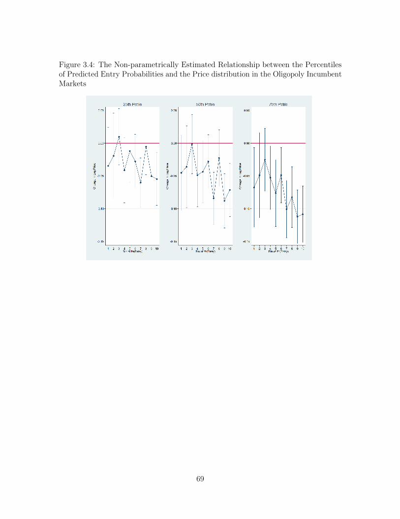
Figure 3.4: The Non-parametrically Estimated Relationship between the Percentilesof Predicted Entry Probabilities and the Price distribution in the Oligopoly IncumbentMarkets
69

Appendices
70
Appendix A Existence and Uniqueness of the Sus-
tainable Price Function
By the definition of z∗, pM violates the sustainability condition for any z > z∗,
i.e.,
πBD(pM)− π(pM) >δ
1− δ(1− FK(zVe)) (πM − πN). (6)
Also,
πBD(pN)− π(pN) <δ
1− δ(1− FK(zVe)) (πM − πN) (7)
for any z > z∗ since πBD(pN )− π(pN ) = 0. Note that πBD(p)− π(p) is continuous on
[pN , pM ]. Then, by the intermediate value theorem, there exists pS(z) ∈ (pN , pM) for
z > z∗ such that
πBD(pS(z))− π(pS(z)) =δ
1− δ(1− FK(zVe)) (πM − πN). (8)
In addition to that, pS(z) is unique since πBD(p)− π(p) is monotonic.
When z goes to infinity, pS(z) = pN , the degenerate solution of the sustain-
ability condition. More specifically,
πBD(pN)− π(pN) = limz→+∞
δ
1− δ(1− FK(zVe)) (πM − πN) = 0. (9)
In sum, there exists pS(z) ∈ [pN , pM) for z > z∗ as a unique solution of the binding
sustainability condition.
71
Appendix B Incentive Compatibility Constraints
in Separating Equilibrium
In a separating equilibrium, the incentive compatibility constraint of h-type is
derived from the condition that the h-type’s profit stream of mimicking the l-type’s
signal pl should be less than or equal to sticking to the h-type’s next best pricing
scheme p∗h(z). That is,
(ICh) : zπh(pl) +δ
1− δ[FK,l(z)zπNh + (1− FK,l(z)) zπMh
]≤ zπh(p
∗h(z)) +
δ
1− δ[FK,h(z)zπNh + (1− FK,h(z)) zπMh
]=⇒ πh(pl) ≤ πh(p
∗h(z))− δ
1− δ(FK,h(z)− FK,l(z))
(πMh − πNh
).
(10)
Similarly, the incentive compatibility constraint of l-type can be represented as follows:
for l-type incumbents, setting pl should be better than or equal to ceasing limit pricing
and then setting p∗l (z), the l-type’s next best strategy, i.e.,
(ICl) : zπl(pl) +δ
1− δ[FK,l(z)zπNl + (1− FK,l(z))zπMl
]≥ zπl(p
∗l (z)) +
δ
1− δ[FK,h(z)zπNl + (1− FK,h(z)) zπMl
]=⇒ πl(pl) ≥ πl(p
∗l (z))− δ
1− δ(FK,h(z)− FK,l(z))
(πMl − πNl
),
(11)
where the LHS is the l-type’s profit stream of limit pricing at pl, and the RHS is the
one of choosing p∗l (z).
72
Appendix C Existence of Non-trivial Limit Pric-
ing
First, I claim that given sufficiently large δ, the l-type non-trivial limit pricing
pLPl (z) = pl(z) ≤ p∗l (z) appears for z ∈ [z1, z2]. If δ is sufficiently large, pl(z) and p∗l (z)
intersect twice at z = z1, z2 because of the non-monotonicity of FK,h(z) − FK,l(z),
i.e., (FK,h(z)− FK,l(z))→ 0 as z → 0 or z →∞, while it is the peak in the middle.
Provided z ∈ [z1, z2], the appearance of pl(z) below p∗l (z) is sufficient to show that
πh(p∗l (z)) ≥ πh(pl(z))
= πh(p∗h(z))− δ
1− δ(FK,h(z)− FK,l(z))
(πMh − πNh
)by ICh.
(12)
The inequality above can be satisfied if δ is sufficiently large as
δ
1− δ≥ 1
FK,h(z)− FK,l(z)· πh(p
∗h(z))− πh(p∗l (z))
πMh − πNh. (13)
Next, I claim that given sufficiently large δ, pl(z) satisfies ICl as well for
z ∈ [z1, z2]. It is sufficient to show that
πl(pl(z)) ≥ πh(pl(z))
= πh(p∗h(z))− δ
1− δ(FK,h(z)− FK,l(z))
(πMh − πNh
)by ICh
≥ πl(p∗l (z))− δ
1− δ(FK,h(z)− FK,l(z))
(πMl − πNl
).
(14)
The last inequality is true if δ is sufficiently large. More specifically, for z ∈ [z1, z2]
δ
1− δ≥ 1
FK,h(z)− FK,l(z)· πl(p
∗l (z))− πh(p∗h(z))
πMl − πNl − (πMh − πNh ). (15)
73
Hence, combining inequality (13) and (15) is a sufficient condition for the existence of
non-trivial limit pricing pl(z) that makes ICh binding and ICl slack. More specifically,
for z ∈ [z1, z2]
δ
1− δ≥ 1
FK,h(z)− FK,l(z)·max
{πl(p
∗l (z))− πh(p∗h(z))
πMl − πNl − (πMh − πNh ),πh(p
∗h(z))− πh(p∗l (z))
πMh − πNh
}.
(16)
Technically speaking, p∗τ (z) for τ ∈ {h, l} is δ-dependent, but it is bounded, i.e.,
p∗τ (z) ∈ [pNτ , pMτ ]. Hence, there exists a sufficiently large δ satisfying the above
inequality.
74
Appendix D The Regularized Logistic Regression
via the Elastic Net Penalty
This section provides more details for the regularized logistic regression via the
elastic net penalty used for the first stage analysis in Section 2.4.2. The regularized
logistic regularization performs a variable selection, considering a bias-variance trade-
off in prediction. As a result, the variable selection can build a parsimonious model
expected to provide better prediction results.
Market characteristics used as predictors are illustrated in the following para-
graphs.
General Characteristics
• Distance: nonstop, round-trip distance of a route;
• Middle Distance: a dummy that is equal to 1 for routes with nonstop, round-trip
distance greater than 500 miles and less than or equal to 2500 miles;
• Long Distance: a dummy that is equal to 1 for routes with nonstop, round-trip
distance greater than 2500 miles;
• Average Population: the log of the geometric mean population of two endpoints
in Metropolitan Statistical Areas (MSAs). Similarly, Average Population2 is the
square of Average Population;
• Big City: a dummy that is equal to 1 if either endpoint airport is in a big city,
following the population-based definition of Gerardi and Shapiro (2009);
• Leisure Destination: a dummy that is equal to 1 if either endpoint airport is in
a leisure destination, following the definition of a leisure destination in Gerardi
75
and Shapiro (2009);
• Slot: a dummy that is equal to 1 if either endpoint airport is a slot-controlled
airport such as John F. Kennedy International Airport (JFK), LaGuardia Airport
(LGA), Ronald Reagan Washington National Airport (DCA), Chicago O’Hare
International Airport (ORD), Los Angeles International Airport (LAX), Newark
Liberty International Airport (EWR), and San Francisco International Airport
(SFO);
• One Primary Airport: a dummy that is equal to 1 if only one endpoint airport
is the largest (in terms of passenger traffic measured in 2018) among multiple
airports in its metropolitan area;
• Two Primary Airports: a dummy that is equal to 1 if both endpoint airports
are primary airports;
• One Secondary Airport: a dummy that is equal to 1 if only one endpoint airport
is the second largest (in terms of passenger traffic measured in 2018) among
multiple airports in its metropolitan area;
• Two Secondary Airports: a dummy that is equal to 1 if both endpoint airports
are secondary airports;
• ConnPass1993: the number of DB1 passengers traveling with a connecting flight
in the first quarter of the route (also ConnPass21993);
• DirPass1993: the number of DB1 passengers traveling with a direct flight in the
first quarter of the route (also DirPass21993);
• HHI DirPass: the average HHI in Phase 1 based on the number of DB1 passengers
traveling with a direct flight, excluding the last four quarters of Phase 1. If
76
the length of Phase 1 is less than or equal to four quarters, the entire Phase 1
quarters are used to calculate the average HHI;
• HHI TotalPass: the average HHI in Phase 1 based on the number of DB1
passengers, excluding the last four quarters of Phase 1. If the length of Phase 1
is less than or equal to four quarters, the entire Phase 1 quarters are used to
calculate the average HHI;
• t0: the first quarter of Phase 2 when Southwest becomes a potential entrant.
The Activity of Legacy Carriers In this group, a variable corresponding to
legacy carrier codes is a dummy equal to 1 if the legacy carrier is an ‘‘active’’ carrier
(see the definition in Section 2.2) during Phase 1 constantly. For example, CO = 1
implies Continental Airlines serves at least 300 DB1 direct in at least 70% of Phase 1.
If carriers are merged on a route during Phase 1, I consider them as active carriers
only if they were serving at least 300 DB1 direct in at least 70% of quarters before
the merger.
The Traffic of Southwest and Incumbents at Endpoints Variables in this
group represent the traffic-related characteristics of Southwest Airlines (WN) and
other incumbent carriers of Phase 1. For WN, I look into the Phase 1 average of
presence at each endpoint airport (defined below) and the Phase 1 average of the
number of routes where WN operates at each endpoint airport. For incumbents, I
only care about the endpoint presence of them.
• WN PresenceO (or WN PresenceD): the log of Phase 1 average proportion of
all passenger traffic in T-100 accounted for by Southwest at the origin (or
destination) airport, excluding the last four quarters of Phase 1. If the length of
77
Phase 1 is less than or equal to four quarters, the entire Phase 1 quarters are
used to calculate the average proportion (also WN Presence2);
• WN RoutesO (or WN RoutesD): the log of Phase 1 average number of routes of
Southwest’s direct service at the origin (or destination) airport, excluding the
last four quarters of Phase 1. If the length of Phase 1 is less than or equal to
four quarters, entire Phase 1 quarters are used to calculate the average routes
(also WN Routes2);
• Incumbent PresenceO (or Incumbent PresenceD): the log of Phase 1 average
of the average proportion of all passenger traffic in T-100 at an origin (or
destination) airport accounted for by the incumbents flying route m, excluding
the last four quarters of Phase 1. If the length of Phase 1 is less than or equal
to four quarters, entire Phase 1 quarters are used to calculate the average
proportion (also Incumbent Presence2),
where O and D stand for origin and destination of a route. Which one is origin or
destination is determined by the ascending order of their airport codes.
The Tuning Parameters I use repeated 10-fold cross-validation with grid search
for the tuning parameters. Accuracy is the metric to select the best parameters in the
validation procedure. Note that most observations have Entry4m = 0 (imbalanced
class). It critically affects the model’s classification performance in that misclassifi-
cation of the minority class is easily ‘‘undervalued’’ by the majority class. I use the
up-sampling method to handle the imbalanced class issue, which randomly replicates
instances in the minority class (Entry4m = 0).
78
The Prediction Performance For comparison regarding classification perfor-
mance, I apply a probit regression to the predictor variables of the regularized logistic
regression. Table D.1 represents a confusion matrix of the probit and regularized
logistic regressions with the test data. The regularized logistic regression better pre-
dicts Southwest’s entry in that its balanced accuracy (0.8844) outweighs the balanced
accuracy of the probit regression (0.7493). It implies that the regularized logistic
regression is less likely to misclassify both classes.
79
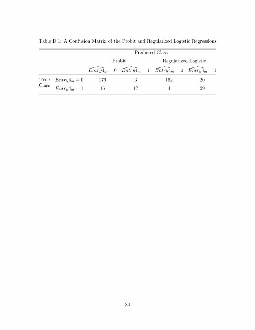
Table D.1: A Confusion Matrix of the Probit and Regularized Logistic Regressions
Predicted Class
Probit Regularized Logistic
Entry4m = 0 Entry4m = 1 Entry4m = 0 Entry4m = 1
TrueClass
Entry4m = 0 179 3 162 20
Entry4m = 1 16 17 4 29
80

Bibliography
Aryal, G., Ciliberto, F., and Leyden, B. (2017). Public communication and tacitcollusion in the airline industry. Working Paper.
Athey, S. and Bagwell, K. (2001). Optimal collusion with private information. RANDJournal of Economics, pages 428--465.
Athey, S., Bagwell, K., and Sanchirico, C. (2004). Collusion and price rigidity. TheReview of Economic Studies, 71(2):317--349.
Bagwell, K. and Ramey, G. (1991). Oligopoly limit pricing. The Rand Journal ofEconomics, pages 155--172.
Bain, J. S. (1949). A note on pricing in monopoly and oligopoly. The AmericanEconomic Review, pages 448--464.
Bernheim, B. D. and Whinston, M. D. (1990). Multimarket contact and collusivebehavior. The RAND Journal of Economics, pages 1--26.
Bonanno, G. (1987). Location choice, product proliferation and entry deterrence. TheReview of Economic Studies, 54(1):37--45.
Borenstein, S. (2004). Rapid price communication and coordination: The airline tariffpublishing case (1994). The Antitrust Revolution: Economics, Competition, andPolicy, 4.
Ciliberto, F. and Williams, J. W. (2014). Does multimarket contact facilitate tacitcollusion? inference on conduct parameters in the airline industry. The RANDJournal of Economics, 45(4):764--791.
Dafny, L. S. (2005). Games hospitals play: Entry deterrence in hospital proceduremarkets. Journal of Economics & Management Strategy, 14(3):513--542.
Eaton, B. C. and Lipsey, R. G. (1979). The theory of market pre-emption: thepersistence of excess capacity and monopoly in growing spatial markets. Economica,46(182):149--158.
81
Ellison, G. and Ellison, S. F. (2011). Strategic entry deterrence and the behaviorof pharmaceutical incumbents prior to patent expiration. American EconomicJournal: Microeconomics, 3(1):1--36.
Evans, W. N. and Kessides, I. N. (1994). Living by the “golden rule”: Multimarketcontact in the us airline industry. The Quarterly Journal of Economics, 109(2):341--366.
Friedman, J. W. (1971). A non-cooperative equilibrium for supergames. The Reviewof Economic Studies, 38(1):1--12.
Gerardi, K. S. and Shapiro, A. H. (2009). Does competition reduce price dispersion?new evidence from the airline industry. Journal of Political Economy, 117(1):1--37.
Goolsbee, A. and Syverson, C. (2008). How do incumbents respond to the threatof entry? evidence from the major airlines. The Quarterly journal of economics,123(4):1611--1633.
Hall, P. and Heckman, N. E. (2000). Testing for monotonicity of a regression meanby calibrating for linear functions. Annals of Statistics, pages 20--39.
Harrington Jr, J. E. (1987). Oligopolistic entry deterrence under incomplete informa-tion. The RAND Journal of Economics, pages 211--231.
Harrington Jr, J. E. (1989). Collusion among asymmetric firms: The case of differentdiscount factors. International Journal of Industrial Organization, 7(2):289--307.
Judd, K. L. (1985). Credible spatial preemption. The RAND Journal of Economics,pages 153--166.
Martin, S. (1995). Oligopoly limit pricing: Strategic substitutes, strategic complements.International Journal of Industrial Organization, 13(1):41--65.
Milgrom, P. and Roberts, J. (1982a). Limit pricing and entry under incompleteinformation: An equilibrium analysis. Econometrica: Journal of the EconometricSociety, pages 443--459.
Milgrom, P. and Roberts, J. (1982b). Predation, reputation, and entry deterrence.Journal of economic theory, 27(2):280--312.
Riley, J. G. (1980). Strong evolutionary equilibrium and the war of attrition. Journalof Theoretical Biology, 82(3):383--400.
Saloner, G. (1987). Predation, mergers, and incomplete information. The RANDJournal of Economics, pages 165--186.
82
Schmalensee, R. (1978). Entry deterrence in the ready-to-eat breakfast cereal industry.The Bell Journal of Economics, pages 305--327.
Seamans, R. C. (2013). Threat of entry, asymmetric information, and pricing. StrategicManagement Journal, 34(4):426--444.
Shin, J. (2021a). Pre-entry price cutting by collusive incumbents with a supergameapproach. Working Paper.
Shin, J. (2021b). Pre-entry price cutting by collusive incumbents with an applicationto the airline industry. Working Paper.
Sweeting, A., Roberts, J. W., and Gedge, C. (2020). A model of dynamic limitpricing with an application to the airline industry. Journal of Political Economy,128(3):1148--1193.
Wilson, R. (1992). Strategic models of entry deterrence. Handbook of game theorywith economic applications, 1:305--329.
83


![THREAT AND ERROR MANAGEMENT [TEM]. · Documentation errors [incorrect data entry or misinterpretation of manuals] Tour of duty problems Management of threats](https://img.pdfslide.us/doc/110x75/5b1e30e77f8b9a62228b5464/threat-and-error-management-tem-documentation-errors-incorrect-data-entry.jpg)