Embed Size (px)
Citation preview

ISBN 978-91-7258-871-4
Doctoral Dissertationin Economics
Stockholm School of Economics Sweden, 2012
Essays on Mathem
atical Economics
Uuganbaatar N
injbat • 2012
Uuganbaatar Ninjbat
Essays on Mathematical Economics

Essays on Mathematical Economics
Uuganbaatar Ninjbat
Akademisk avhandling
som för avläggande av ekonomie doktorsexamen vid Handelshögskolan i Stockholm framläggs för offentlig granskning
tisdagen den 23 oktober 2012, kl 15.15 i Peter Wallenberg Salen, Handelshögskolan,
Sveavägen 65, Stockholm

ESSAYS ON MATHEMATICAL ECONOMICS


Essays on Mathematical Economics
Uuganbaatar Ninjbat

Dissertation for the Degree of Doctor of Philosophy, Ph.D.
Stockholm School of Economics 2012
Keywords: Optimal schedules, FCFS, The Leontief preferences, Approval Voting, Young’s
theorem, May’s theorem, Strategy-proofness, Options sets, Impossibility theorem
ESSAYS ON MATHEMATICAL ECONOMICS
© SSE and Uuganbaatar Ninjbat, 2012
ISBN 978-91-7258-871-4
Printed in Sweden by:
Ineko, Göteborg 2012
Distributed by:
The Research Office
Stockholm School of Economics
Box 6501, SE-113 83 Stockholm, Sweden
www.hhs.se
iv

Preface
This report is a result of a research project carried out at the department of Economics
at the Stockholm School of Economics (SSE).
This volume is submitted as a doctor’s thesis at SSE. The author has been entirely free
to conduct and present his research in his own ways as an expression of his own ideas.
SSE is grateful for the financial support which has made it possible to fulfill the project.
Goran Lindqvist
Director of Research
Stockholm School of Economics
Magnus Johannesson
Professor and Head of the Department of
Economics
Stockholm School of Economics
v


Contents
1 Introduction 3
2 Optimality of First-Come-First-Served: A Unified Approach 13
2.1 Introduction . . . . . . . . . . . . . . . . . . . . . . . . . . . . . . . . . . . 13
2.2 The set up . . . . . . . . . . . . . . . . . . . . . . . . . . . . . . . . . . . . 15
2.3 Single server systems . . . . . . . . . . . . . . . . . . . . . . . . . . . . . . 16
2.4 Multi server systems with equal processing time . . . . . . . . . . . . . . . 21
2.5 Conclusion . . . . . . . . . . . . . . . . . . . . . . . . . . . . . . . . . . . . 22
3 An Axiomatization of the Leontief Preferences 27
3.1 Introduction . . . . . . . . . . . . . . . . . . . . . . . . . . . . . . . . . . . 27
3.2 The preliminaries . . . . . . . . . . . . . . . . . . . . . . . . . . . . . . . . 29
3.3 The characterization theorem . . . . . . . . . . . . . . . . . . . . . . . . . 30
3.4 Conclusions . . . . . . . . . . . . . . . . . . . . . . . . . . . . . . . . . . . 34
3.5 Appendix . . . . . . . . . . . . . . . . . . . . . . . . . . . . . . . . . . . . 35
4 Remarks on Young’s Theorem 41
4.1 Introduction . . . . . . . . . . . . . . . . . . . . . . . . . . . . . . . . . . . 41
4.2 The preliminaries . . . . . . . . . . . . . . . . . . . . . . . . . . . . . . . . 42
4.3 The axioms for scoring rules when m = 2 . . . . . . . . . . . . . . . . . . . 43
4.3.1 Two remarks on Young’s theorem . . . . . . . . . . . . . . . . . . . 43
4.3.2 Allowing for indifferences in voters’ preferences . . . . . . . . . . . 46
4.4 Final comments . . . . . . . . . . . . . . . . . . . . . . . . . . . . . . . . . 50
5 Approval Voting without Faithfulness 55
5.1 Introduction . . . . . . . . . . . . . . . . . . . . . . . . . . . . . . . . . . . 55
5.2 Characterization . . . . . . . . . . . . . . . . . . . . . . . . . . . . . . . . 56
5.3 Final Remarks . . . . . . . . . . . . . . . . . . . . . . . . . . . . . . . . . . 60
vii

CONTENTS
6 Another Direct Proof for the Gibbard-Satterthwaite Theorem 63
6.1 Introduction . . . . . . . . . . . . . . . . . . . . . . . . . . . . . . . . . . . 63
6.2 The preliminaries . . . . . . . . . . . . . . . . . . . . . . . . . . . . . . . . 64
6.3 The main result and the proof . . . . . . . . . . . . . . . . . . . . . . . . . 65
6.4 Final remarks . . . . . . . . . . . . . . . . . . . . . . . . . . . . . . . . . . 71
7 Symmetry vs. Complexity in Proving the Muller-Satterthwaite Theo-
rem 75
7.1 Introduction . . . . . . . . . . . . . . . . . . . . . . . . . . . . . . . . . . . 75
7.2 The preliminaries . . . . . . . . . . . . . . . . . . . . . . . . . . . . . . . . 77
7.3 The proofs for the baseline case . . . . . . . . . . . . . . . . . . . . . . . . 77
7.4 Sufficiency of proving the M-S Theorem for n = 3 . . . . . . . . . . . . . . 81
7.5 Final comments . . . . . . . . . . . . . . . . . . . . . . . . . . . . . . . . . 84
viii

Acknowledgements
During my Ph.D studies at SSE, I have been under academic and administrative support
of two persons: Mark Voorneveld and Richard Friberg. The journey started with Mark
back in 2009. After it took off with him we did the landing with Richard. Without their
support thesis would not be here at this final stage. So, thanks to both of them.
I am also thankful to Magnus Johannesson, who had two important administrative
duties during this time: initially as our Ph.D program coordinator, and later as our
department chair. In 2009 Jorgen Weibull asked me to be his TA for the Math-1 course.
I think that it was a rewarding experience for me and I am thankful to him for giving me
this opportunity.
Our administrative secretaries, Ritva Kiviharju, Carin Blanksvard and Lilian Oberg,
were very kind and helpful whenever I knocked their door for different reasons ranging
from preparation of a certain official documentation to matters related to the kitchen at
the 8’th floor. I am thankful to them for their kindness.
My fellow students were very helpful and willing to share their own experiences when-
ever I turned to them on more personal matters related to local and regional issues.
Especially, Karin and Anna were the most reliable sources when it comes to the arrange-
ments of all such local matters.
Finally, financial support from the Wallander-Hedelius foundation is gratefully ac-
knowledged.
1


Chapter 1
Introduction
This thesis consists of six single authored research papers. Five out of the six papers are
published as journal articles:
1. Optimality of first-come-first-served: a unified approach, Mongolian Mathematical
Journal, 2011, 15: 45-53. (included in Chapter 2)
2. An axiomatization of the Leontief preferences, to appear in Finnish Economic Papers,
2012, 25 (1). (included in Chapter 3)
3. Remarks on Young’s theorem, Economics Bulletin, 2012, 32 (1): 706-714. (included
in Chapter 4)
4. Approval voting without faithfulness, 2012. (included in Chapter 5)
5. Another direct proof for the Gibbard-Satterthwaite theorem, Economics Letters, 2012,
116 (3): 418-421. (included in Chapter 6)
6. Symmetry vs. complexity in proving the Muller-Satterthwaite theorem, Economics
Bulletin, 2012, 32 (2): 1434-1441. (included in Chapter 7)
The first paper is on queues and schedules. Queueing theory mathematically analyzes
certain aspects of congestion situations that often arise in service and manufacturing
industries as well as in communication networks. It is a subfield of Operations Research
and Industrial and Systems Engineering studies. A related field to queueing theory is
scheduling theory, which studies the problem of assigning, over time, a certain number
of jobs to a certain number machines so that the jobs get processed by the machines
according to this assignment.
3

CHAPTER 1. INTRODUCTION
The main difference between these two fields is that the former has a stochastic setting,
while the latter usually has a deterministic setting. However, the problem of finding the
best allocation of jobs (or customers) to machines (or servers) arises in both disciplines. In
particular, the main theme of scheduling theory is, under given objectives and constraints,
to find the optimal such allocations.
Within this context, among other problems, the problems of investigating the optimal-
ity properties of the well known schedules (or queue disciplines), such as first-come-first-
served (FCFS), last-come-first-served and shortest-remaining-processing-time, are stud-
ied. Such problems are usually solved with the techniques of optimization theory, i.e.
Linear, Integer and Dynamic Programming methods.
In our paper, we suggest an alternative approach to investigate optimality properties
of FCFS schedule. We demonstrate our approach in a single and identical m parallel
machine scheduling settings. Using our approach we verify that FCFS is optimal for the
following ”bottleneck” problems: max of completion time, max of flow time and max
of waiting time. The underlying idea of our approach is to compare schedules over the
last busy period before the system reaches to its peak under FCFS. Then, the optimality
proof pins down to comparison of sums of real numbers and hence, our approach leads to
simple, direct and self-contained proofs for the optimality results related to FCFS.
On the other hand, there are two standard approaches used in scheduling literature to
solve these problems. The first one uses the ”interchange argument,” which is a method
based on the following reasoning: an optimal schedule is characterized by the property
that interchanging two jobs does not improve the value of the objective function. The
second method refers to a classic result by Hardy, Littlewood and Polya when solving this
problem (see for instance, Section 5.3 in Pinedo, 2008).
The former of these two is perhaps more general. It can be used for solving other
scheduling problems, and can also be applied to a stochastic setting. The key aspect of
this method is that it is related to a general principle in optimization theory: ”optimality
can be studied through variation.” The latter is, on the other hand, more delicate and it
gives the result immediately. It is also related to another common and powerful technique
in optimization theory, the Majorization technique (see for instance, Marshall, et al.,
2009). In comparison, according to our opinion, our approach is more direct than the
other two.
Given that scheduling problems are renowned for their complexities (see Brucker, 2007;
Brucker and Knust, 2011), a new approach to investigate such problems can be useful.
Moreover, in a computer environment, applying the interchange argument can be very
4

costly as it is based on binary comparisons. In such cases, a more direct approach is
preferable. In particular, if the problem is to determine whether FCFS is better than
some other given schedule, our approach is certainly more efficient than the others.
The second paper is on choice theory. We give an axiomatic characterization of weak
preferences as the Leontief preferences (or the maximin preferences). The Leontief pref-
erences frequently appear in economic literature. In consumer choice theory they are the
most useful tool to analyze the consumer choice when commodities are complements, i.e.
when the value of each commodity positively depends on the relative abundance of the
others. In social choice theory they appear in the formalization of Rawlsian theory of
justice (see Rawls, 1971).
It is also closely related to the well known minimax decision criteria in statistical
decision theory. A decision maker whose objective is to minimize the maximum loss (or
regret) follows such a decision rule. This rule has received wide attention after the works
of A.Wald and L.J.Savage (for a short overview, see Stoye, 2009). On the other hand,
the same decision maker, when her objective is to maximize the minimum gain instead,
follows the maximin decision rule, i.e. she has the maximin preferences. Hence, as long
as ”gain” and ”loss” are related, so are these decision rules.
The key axiom in our axiomatization is upper consistency, which is based on the fol-
lowing trinary comparison: given two alternatives, under which condition would a decision
maker weakly prefer a third alternative to at least one of the two? Then, along with two
other rather common axioms (symmetry and local non-satiation), specifying such a con-
dition leads us to the maximin preferences. Hence, our analysis suggests that, despite of
its rich philosophical and decision theoretical content, the maximin preferences have a
simple structure in terms of preferences.
The last four papers are on voting and social choice theory. One of the main themes
of this field is to find out which choice aggregation procedures have which properties.
Along this line there are both positive, in the sense of possibility or existence of certain
procedures satisfying certain properties, and negative, in the sense of impossibility or
non-existence of such procedures, results in this literature. We will consider both kinds
of results in our papers (see Chapters 4 to 7).
The third paper is on axiomatization of social choice scoring rules. Scoring rules
constitute a broad class of voting methods which share the following common structure:
voters rank the alternatives arbitrarily, and each alternative, depending on its position in
each voter’s ranking, receives a score (a real number), and the alternatives that collect
the highest score are chosen. A case in point is the well known Borda rule, which is a
5

CHAPTER 1. INTRODUCTION
scoring rule with the scores of 0, 1, ..., m− 1, where m is the number of alternatives, and
the i’th best alternative receives m− i score.
In a variable electorate setting, i.e. when the number of voters is not fixed, Smith
(1973) and Young (1975) axiomatized scoring rules with four axioms: anonymity, neu-
trality, continuity and consistency. The first two axioms represent the idea that the voters
and the alternatives are to be treated equally. However, the key axioms in their charac-
terization are the last two, continuity and consistency. The continuity axiom is a kind of
”domination by large numbers” principle and it says that, when a subgroup of voters is
replicated sufficiently many times the enlarged group eventually chooses the alternatives
which are in the subgroup’s choice. The consistency axiom says that, when there are two
disjoint groups whose choices overlap or agree to some extend, and when these groups
come together, the new group’s choice must be those alternatives which both groups had
in common in their choices (for more discussions, see Chapter 9 in Moulin, 1988).
In our paper, we provide some additional results related to the axiomatization of
scoring rules. We first show that when there are two alternatives, the continuity axiom
in the above characterization is unnecessary. We then provide a rather complete analysis
of the two alternative case by showing that,
(a) the smaller set of axioms (i.e. anonymity, neutrality and consistency) characterize
scoring rules even if voters are allowed to be indifferent between the alternatives,
(b) one can obtain a variant May’s theorem (which gives an axiomatic characterization
of majority rule) from the result in (a), and
(c) in each of these results, the axioms of neutrality and cancellation can be used inter-
changeably.
The fourth paper is on Approval Voting (AV). AV is considered as a simple yet powerful
voting method. Under AV, each voter divides alternatives into two classes, those she
approves and those she does not, and the approved alternatives are casted in her ballot.
After collecting all ballots, the most approved alternatives are chosen as the winners.
Among its advantages perhaps the most notable one is that it reduces voters’ incentives
to vote insincerely, in part, by giving them rich and flexible ballot choices (see Brams
and Fishburn, 1978). Moreover, according to Brams and Fishburn (2005), the other
advantages of AV are
• it helps to elect the strongest candidate, in the sense of Condorcet winner : a candi-
date who would win against each of the other candidates in a two candidate election
under majority rule,
6

• it reduces negative campaigning,
• it increases voter turnout, and
• it gives minority candidates their proper due.
Fishburn (1978) showed that AV is the only ballot aggregation function satisfying the
axioms of neutrality, consistency, cancellation and faithfulness. Notice that the first two
axioms already appeared in the axiomatization of scoring rules discussed above. Can-
cellation requires that when all alternatives receive the same number of votes, the ballot
aggregation function should choose all of them. Faithfulness requires that when group’s
profile consists of a single voter’s ballot, then those alternatives in her ballot are to be
chosen at that profile.
In our paper, we investigate the implications of dropping the axiom of faithfulness in
Fishburn (1978)’s axiomatization. We show that if one drops it, then there are only three
ballot aggregation functions satisfying the remaining axioms (neutrality, consistency and
cancellation), namely,
• AV, and
• a function that chooses the least approved alternatives, which we call as Inverse
Approval Voting, and
• a function that chooses the whole set of alternatives at all profiles.
Hence, our finding suggests that the primary role of faithfulness in Fishburn (1978)’s
axiomatization is to distinguish AV from two other functions, one of which has a trivial
structure, while the other has a similar but opposite structure as AV. Finally, it is worth
to mention that there is an interesting similarity between our result and Wilson’s impos-
sibility theorem (see Wilson, 1972), which is obtained as a consequence of dropping the
Pareto axiom in Arrow’s impossibility theorem.
The last two papers are on social choice impossibility theorems. Impossibility theo-
rems are special kind of axiomatization results which show that a set of (desirable) axioms
are incompatible when they put together. The most well known example of such result is
Arrow’s Impossibility Theorem, which states that, when there are at least three alterna-
tives, there is no social welfare function satisfying the axioms of independence of irrelevant
alternatives, Pareto efficiency and non-dictatorship. The other well known impossibility
theorems are the Gibbard-Satterthwaite theorem and the Muller-Satterthwaite theorem.
The former of the two shows that there is no social choice function satisfying the axioms of
7

CHAPTER 1. INTRODUCTION
unanimity, strategy-proofness (non-manipulability) and non-dictatorship, while the latter
is a similar result obtained by replacing strategy-proofness with (Maskin) monotonicity.
These theorems received much attention since their initial appearances. For example,
several extensions and generalizations are obtained, their interconnections are analyzed,
as well as several ways of proving these kind of theorems are discovered (for a survey
see, Campbell and Kelly 2002; Barbera, 2011). However, they are often mentioned as
”paradoxes,” which indicates that more work needs to be done on these results. Indeed,
some authors already suggested that any amount of mystery in these results needs to be
”demystified” (see Saari, 2008).
In the literature, impossibility theorems are usually presented as characterization the-
orems of the following type: a social choice function satisfies all but the last axiom (non-
dictatorship) if and only if it is a dictatorial social choice function (i.e. a function whose
choice coincides with a certain individual’s choice at all the time), which is then incon-
sistent with the remaining axiom. Moreover, a common approach to prove such results
works as follows. In order to prove that a function satisfying a set of axioms is dictatorial,
first, a subset of the set of individuals containing a dictator (a distinguished individual
who determines the group’s choice) is defined or identified (e.g., decisive coalition, piv-
otal voter etc.). Then, certain properties of that set are investigated, and eventually it
is shown that this set is a singleton. A classic example of such approach is Sen’s proof
of Arrow’s Impossibility Theorem using the so called Field Extension Lemma and Group
Contraction Lemma (see Sen, 1986). The other well known cases of this common approach
are Barbera’s pivotal voters approach (Barbera 1980, 1983), and Geanakoplos’ extremely
pivotal voters approach (Geanakoplos, 2005).
In the fifth paper we propose an alternative approach to prove this kind of results.
We consider the case of the Gibbard-Satterthwaite (impossibility) theorem. The essence
of our approach is that, in contrast to the common approach described above, we focus
on the individuals who are not candidates for a dictator. More specifically, it consists
of two steps. First, we show that when a social choice function is strategy-proof and
unanimous, at any given profile, if an individual’s most preferred alternative differs from
the social choice, then she can not change the social choice at that profile by changing
her preferences. Then, in the second step we deduce the Gibbard-Satterthwaite theorem
from this result.
We believe that our approach can be seen as a complementary (or dual) approach to
the other approaches that focus on the potential candidates of a dictator of a social choice
function. Moreover, in our opinion, it provides some additional insights on social choice
8

impossibility results.
The last paper is on the Muller-Satterthwaite (impossibility) theorem. We provide an
induction proof of the theorem. We first prove it in the baseline case of two persons and
three alternatives. Then, we show that it actually suffices to prove this result for the case
of three alternatives with arbitrary N individuals, as it then can easily be extended to
the general case of finite but more than three alternatives. We then complete our proof of
the Muller-Satterthwaite theorem by showing that the result holds for the decisive case
of three alternatives by induction on N .
In our proof, we explicitly use the symmetry property (or the neutrality axiom) which
is hidden in the definition of a social choice function. This allows us to see the underlying
structure of the Muller-Satterthwaite theorem more clearly. In particular, the mono-
tonicity axiom, which is central in this result, is above all an order theoretical notion:
it defines, with respect to each alternative, a preorder on the set of preference profiles.
In this respect, our paper is a step toward putting the order theoretical aspects of the
Muller-Satterthwaite theorem in front, and more work along this direction is a subject to
further research.
9


Bibliography
[1] Barbera, S. (1980) ”Pivotal voters: a new proof of Arrow’s impossibility theorem.”
Economics Letters 6: 13-16.
[2] Barbera, S. (1983) ”Strategy-proofness and pivotal voters: a direct proof of the
Gibbard-Satterthwaite theorem.” International Economics Review 24: 413-418.
[3] Barbera, S. (2011) ”Strategy-proof social choice.” In Handbook of Social Choice and
Welfare, Vol. 2. Eds. K.J.Arrow, A.K.Sen and K.Suzumura, North-Holland: Amster-
dam.
[4] Brams, S.J., and F.C. Fishburn (1978) ”Approval Voting.” The American Political
Science Review 72 (3): 831-847.
[5] Brams, S.J., and F.C. Fishburn (2005) ”Going from theory to practice: the mixed
success of Approval Voting.” Social Choice and Welfare 25: 457-474.
[6] Brucker, P. (2007) Scheduling Algorithms, 5th edition, Springer.
[7] Brucker, P and S.Knust (2010) Complex Scheduling, Springer.
[8] Campbell, D.E and J.S. Kelly (2002) ”Impossibility theorems in the arrovian frame-
work.” In: Handbook of Social Choice and Welfare, Vol. 1. Eds. K.J.Arrow, A.K.Sen
and K.Suzumura, North-Holland: Amsterdam.
[9] Fishburn, P.C. (1978) ”Symmetric and consistent aggregation with dichotomous vot-
ing.” In: Aggregation and Revelation of Preferences, J-J. Laffont (eds.), North Hol-
land: Amsterdam.
[10] Geanakoplos, J. (2005) ”Three brief proofs of Arrow’s impossibility theorem.” Eco-
nomic Theory, 26: 211-215.
[11] Marshall, A.W., Olkin, I. and B.C.Arnold (2009) Inequalities: Theory of Majorization
and Its Applications, 2nd edition, Springer.
11

BIBLIOGRAPHY
[12] Moulin, H. (1988) Axioms of Cooperative Decision Making, Cambridge University
Press.
[13] Pinedo, M.L. (2008) Scheduling: Theory, Algorithms and Systems, 3rd edition,
Springer.
[14] Rawls, J. (1971) A Theory of Justice, Harvard University Press.
[15] Saari, D. (2008) Disposing Dictators, Demystifying Voting Paradoxes: Social choice
analysis, Cambridge University Press.
[16] Sen, A. (1986) ”Social Choice Theory.” In: Handbook of Mathematical Economics,
Vol. 3. Eds. K.J.Arrow and M.D.Intriligator, North-Holland: Amsterdam.
[17] Smith, J.H. (1973) ”Aggregation of preferences with variable electorate” Economet-
rica 41: 1027-1041.
[18] Stoye, J. (2009) ”Minimax.” In: The New Palgrave Dictionary of Economics, S.N.
Durlauf and L.E.Blume (eds.), online edition.
[19] Wilson, R. (1972) ”Social choice theory without the Pareto principle.” Journal of
Economic Theory 5: 478-486.
[20] Young, H.P. (1975) ”Social choice scoring functions.” SIAM J. Appl. Math. 28: 824-
838.
12

Chapter 2
Optimality of
First-Come-First-Served: A Unified
Approach1
Abstract: This paper provides a unified approach that can directly verify the follow-
ing results related to First-Come-First-Served (FCFS): (a) in the case of a single server
system, FCFS is optimal for max of C (completion time) and max of F (flow time), (b)
in the case of a multi server system with identical servers, when customers have the equal
processing time, any optimal discipline for the total (sum) of C, F and W (waiting time)
has the same service starting times as FCFS, and (c) in the latter case, FCFS is optimal
for max of C, max of F and max of W .
Keywords: Optimality of FCFS, Optimal non-preemptive queue disciplines, Parallel
machine scheduling with equal processing time.
2.1 Introduction
In queueing models, FCFS is often assumed to be the queue discipline. Moreover, FCFS
is very common in real life situations such as the grocery stores. This paper aims
to (re)investigate certain optimality properties of this commonly used queue discipline.
There are several results on the optimality of FCFS in queueing literature (see Gittins
[6], Foss [4], Doshi and Lipper [3], Daley [2], Wolf [12], Righter and Shanthikumar [9], Liu
and Towsley [8], Foss and Chernova [5]).
1Published in Mongolian Mathematical Journal, 2011, 15: 45-53.
13

CHAPTER 2. OPTIMALITY OF FIRST-COME-FIRST-SERVED: A UNIFIED
APPROACH
Generality of these results necessarily depends on their setting: properties of the queue-
ing system, class of disciplines among which the comparison is made and the optimality
criterion that is considered. For instance, Gittins [6] shows that in (GI/GI/m) queues, if
the processing times are i.i.d across customers, then the expected waiting time for a typ-
ical customer in steady state is minimum under FCFS among all non-preemptive queue
disciplines.2 More recent works provide rather general results: in (G/GI/m) queues, if
the processing times are i.i.d across customers, the expected value of any Schur convex
function of customer waiting times and total workload after arrival of each customer, and
of any symmetric and convex function of customer flow times are minimum under FCFS,
among all non-preemptive queue disciplines (see Foss [4], Daley [2], Liu and Towsley [8],
Towsley [11], Foss and Chernova [5]).
In this paper we treat the discipline design problem as a scheduling problem. Ac-
cordingly, we use performance measures used in scheduling theory to evaluate different
queue disciplines: total and max of completion time, flow time and waiting time (C, F ,
W ), and all of our results can be interpreted in the context of (n/m) parallel machine
scheduling problem. Our main findings are as follows. First, in Theorem 2.2 in Section
2.3 we show that, in the case of a single server system, FCFS minimizes max of C and
max of F . We then consider systems with identical customers, i.e. with equal processing
times. However, all performance measures that we consider are convex and symmetric
(hence, Schur convex) and the equal processing time case is a special case of that being
i.i.d. But in Theorem 2.3 in Section 2.3 we show that, when all customers have the same
processing time, not only FCFS is optimal for the the sum of C, F,W , but any optimal
schedule has the same service starting times as FCFS. Then, in Theorem 2.5 in Section
2.3 we also show that, in that case FCFS is optimal for max of W . Finally, in Theorem
2.7 and 2.8 in Section 2.4, we extend results in Theorem 2.3 and 2.5 in Section 2.3 to the
case of a multi server system with identical servers.
Most of our results are known in scheduling literature. For instance, results in Theorem
2.2 are well known in scheduling theory (see Lawler [7], Baker and Trietsch [1]). Results
in Theorem 2.3 (a) and 2.7 follow from ”optimality of greedy schedules,” whereas results
in Theorem 2.5 and 2.8 follow from a more general result in Simmons [10]. However,
our proof technique is based on a recursive reasoning and it is different than the other
popular techniques: interchange argument, forward and backward induction, majorization
2In queueing theory, so called Kendall’s notation, A/B/m, is often used to describe queueing systems.A describes the arrival time distribution, B describes the service times distribution and the last entry,m describes the number of service channels. G stands for general and GI stands for general independentdistributions.
14

2.2. THE SET UP
argument and linear and dynamic programming. It is based on a simple observation that
”in order to show optimality of FCFS for max (bottleneck)-problems, it suffices to compare
feasible schedules over the last busy period before system reaches its peak under FCFS,”
and provides a direct, self-contained and unified approach, used thoroughly in proving
Theorem 2.2, 2.5, 2.8 in Section 2.3 and 2.4.
In the next section we introduce our notation and main definitions. In Section 2.3, we
consider single server systems and in Section 2.4 we consider multi server systems with
identical servers and the last section concludes.
2.2 The set up
Let there be n ∈ N customers J = {1, 2, ..., n} and a single server. Each customer i ∈ J
has a processing time pi ≥ 0 and an arrival time ti ≥ 0 and let p = (p1, ..., pn) ∈ Rn+
and t = (t1, ..., tn) ∈ Rn+ be the corresponding vectors. Without loss of generality we may
assume that 0 ≤ t1 ≤ · · · ≤ tn. A schedule s = (s1, . . . , sn) ∈ Rn+ for a given (p, t) ∈
Rn+ × Rn
+ assigns to each customer i ∈ J a starting time si ≥ 0 when the server begins
to process it. It is feasible if processing of a customer does not start before his arrival,
si ≥ ti, i ∈ J , and the server does not process more than one customer simultaneously,
∀i, j ∈ J with i 6= j, [si, si + pi) ∩ [sj, sj + pj) = ∅. First-come-first-served-schedule
(FCFSS) is a schedule s∗ that processes all jobs in the order of their arrival and does
so as soon as possible: s∗1 = t1 and s∗i = max{s∗i−1 + pi−1, ti} for i = 2, . . . , n. Note
that, according to the above definition we only consider permutation schedules without
preemption, but we allow the server to stay idle when there are customers available for
the service. From now on we only consider feasible schedules and we first verify that the
FCFSS is feasible.
Proposition 2.1 s∗is feasible for any (p, t) ∈ Rn+ × Rn
+.
Proof. We can express the feasibility condition above as follows: si ≥ ti, i ∈ J , and
∀i, j ∈ J such that i 6= j, if si < sj, then si+pi ≤ sj . Then, by definition s∗ satisfies both
of these conditions. �
A queue discipline is defined as a complete contingent plan of schedules. More formally,
a queue discipline is a mapping q : Rn+ × Rn
+ → Rn+ which assigns to each (p, t) ∈
Rn+ × Rn
+ a feasible schedule s. The FCFS is a queue discipline q∗ such that ∀(p, t) ∈
Rn+ × Rn
+, q∗(p, t) = s∗. The following performance measures are commonly used in
15

CHAPTER 2. OPTIMALITY OF FIRST-COME-FIRST-SERVED: A UNIFIED
APPROACH
both queueing and scheduling theory. The flow time, the completion time and the
waiting time for customer i ∈ J under schedule s are the time that he spends in the
queueing system, the time that is needed before he gets the service completed and the
time that he waits in the queue until he gets the service, respectively. The corresponding
formulas are: Fi(s) = si + pi − ti, Ci(s) = si + pi and Wi(s) = si − ti. The sum
(total) and the maximum of these measures are defined as usual: F (s) =∑n
1 Fi(s),
Fmax(s) = max{F1(s), ..., Fn(s)}; C(s) =∑n
1 Ci(s), Cmax(s) = max{C1(s), ..., Cn(s)};
W (s) =∑n
1 Wi(s), Wmax(s) = max{W1(s), ...,Wn(s)}.
A schedule s is an optimal schedule for the performance measure M if there is no
other schedule s′ such that M(s′) < M(s) and a queue discipline q is optimal for
M if ∀(p, t) ∈ Rn+ × Rn
+, q(p, t) is optimal for M . Finally, the following permutation
defined for any set of finitely many real numbers is very useful in our proofs. Let α =
(αk+1, ..., αk+m) ∈ Rm+ be a set of m nonnegative real numbers and let απ = (απ1 , ..., απm
)
a permutation of α. Then we call απ as ranking of α if απi≤ απi+1
for i = 1, ..., m− 1.
2.3 Single server systems
Theorem 2.2 Consider a single server system and let (p, t) ∈ Rn+ × Rn
+ be arbitrary.
Then q∗ is optimal for Cmax and Fmax.
Proof. For the first claim, we need to prove that, given (p, t) ∈ Rn+ × Rn
+, for any
schedule s, Cmax(s) ≥ Cmax(s∗). By definition, s∗i = max{s∗i−1 + pi−1, ti} for i = 2, ..., n,
which implies that s∗i + pi ≥ s∗i−1 + pi−1, for i = 2, ..., n and hence, Cmax(s∗) = s∗n + pn.
Let us define j = max{i : 1 ≤ i ≤ n, s∗i = ti}. So, j is the the last customer in J who
gets the service at his arrival under s∗. Note that j is well defined since s∗1 = t1. For an
arbitrary schedule s, consider α = (sj , ..., sn) and its ranking απ = (sπ1, ..., sπn−j+1). By
feasibility, si ≥ ti ≥ tj for i = j, ..., n, and sπn−j+1+ pπn−j+1
≥ sπn−j+ pπn−j
+ pπn−j+1≥
... ≥ tj +∑n
i=j pi. By definition, Cmax(s) ≥ sπn−j+1+ pπn−j+1
. But since s∗i = s∗i−1 + pi−1
for i = j +1, ..., n and s∗j = tj , Cmax(s∗) = tj +
∑n
i=j pi. Hence, Cmax(s) ≥ Cmax(s∗). This
proves the first claim.
For the second claim, we need to prove that, given (p, t) ∈ Rn+×Rn
+, for any schedule s,
Fmax(s) ≥ Fmax(s∗). By definition, F1(s
∗) = p1 and for i = 2, ..., n, Fi(s∗) = s∗i + pi − ti =
max{s∗i−1 + pi−1, ti} − ti + pi = max{s∗i−1 + pi−1 − ti, 0} + pi. Let k ∈ J be such that
Fmax(s∗) = Fk(s
∗). Let us define j = max{i : 1 ≤ i ≤ k, s∗i = ti}. So, j is the the last
customer in {1, ..., k} who gets the service at his arrival under s∗. Note that j is well
defined since s∗1 = t1. Then by definition, Fk(s∗) = s∗k + pk − tk = tj +
∑k
i=j pi − tk.
16

2.3. SINGLE SERVER SYSTEMS
For an arbitrary schedule s = (s1, ..., sn), consider α = (sj, ..., sk) and its ranking
απ = (sπ1 , ..., sπk−j+1). Note that tj ≤ tπ1 ≤ sπ1 and tπk−j+1
≤ tk and by feasibility we
conclude that Fπk−j+1(s) = sπk−j+1
+ pπk−j+1− tπk−j+1
≥ sπk−j+ pπk−j
+ pπk−j+1− tπk−j+1
≥
... ≥ sπ1 +∑k
i=j pi − tπk−j+1≥ tj +
∑k
i=j pi − tk = Fk(s∗). Since Fmax(s) ≥ Fπk−j+1
(s), this
completes the proof. �
Results in Theorem 2.2 show that s∗ is always optimal for Cmax and Fmax. The
following example shows that for the other performance measures, such a general result
does not hold.
Example 2.1 Let n = 2 and t = (0, 1) and p = (10, 1). Consider schedule s = (2, 1).
Then F (s) = 13 < F (s∗) = 20; C(s) = 14 < C(s∗) = 21; W (s) = Wmax(s) = 2 < 9 =
W (s∗) = Wmax(s∗). ⊳
However, if all customers have the equal processing time, s∗ is optimal for all of these
performance measures.
Theorem 2.3 Let all customers have the equal processing time, pi = p0 ∈ R+, i ∈ J .
Then,
(a) schedule s is optimal for F (s),W (s)and C(s) if and only if sπi= s∗i for all i ∈ J ,
where sπ = (sπ1, ..., sπn) is the ranking of s, and
(b) s∗ is optimal for the performance measures in (a). Moreover, s∗ is the unique optimal
schedule if and only if t ∈ Rn+ is such that ti + p0 < ti+2, for i = 1, ..., n− 2.
Proof. (a) Note that the objectives differ by a constant, hence the optimal schedules
coincide. Each objective take its minimum value whenever∑
si is at its minimum. Let s
be an arbitrary schedule.
For the if part, it suffices to show that∑
s∗i ≤∑
si. Consider the ranking sπ =
(sπ1, ..., sπn) of s. Since sπ is a permutation of s,
∑
sπi=
∑
si. Note that by feasibility,
sπj≥ tj for all j = 1, ..., n since there must be at least j customers have arrived in order
πj to be the j′th customer to be served. In particular, sπ1 ≥ t1 = s∗1. For 2 ≤ i ≤ n,
if sπi−1≥ s∗i−1, then it is also true that sπi
≥ s∗i since sπi≥ sπi−1
+ p0 ≥ s∗i−1 + p0 and
sπi≥ ti. But since sπ1 ≥ s∗1, we conclude that sπi
≥ s∗i , i ∈ J . Hence,∑
sπi≥
∑
s∗i .
For the only if part, suppose s is optimal. Then it must be the case that∑
sπi=
∑
s∗iand since it is also true that sπi
≥ s∗i , i ∈ J , the equality of the two sums is possible only
if each term in the sum is equal. This completes the proof.
17

CHAPTER 2. OPTIMALITY OF FIRST-COME-FIRST-SERVED: A UNIFIED
APPROACH
(b) The optimality of s∗ is trivial from (a). Note that, if s is an optimal schedule,
then sπ1 = s∗1 = t1, which implies that π1 = 1 since it is possible to assign t1 only to the
customer 1. For the if part, suppose t1 + p0 < t3. Since t2 < t3, we conclude that t3 > s∗2.
But for an optimal schedule s, the only customer that can be scheduled at sπ2 = s∗2 is the
customer 2 since no other customer is available at s∗2. Hence, for any optimal schedule s,
π2 = 2. Similarly, we conclude that πi = i for i = 3, ..., n. Hence, if s is optimal, then
s = s∗.
For the only if part, let s∗ be the only optimal schedule and let there be j ∈ {1, ..., n−2}
such that tj + p0 > tj+2. Consider schedule s such that it agrees with s∗ in all positions
but (j + 1)′th and (j + 2)′th : sπi= s∗i for i ∈ J and πi = i for i ∈ J\{j + 1, j + 2} and
πj+1 = j + 2 and πj+2 = j + 1. Then by construction s is optimal and s 6= s∗, which
contradicts to the uniqueness of s∗. �
The theorem above can be interpreted as: when all customers have the same processing
time, the optimal schedule is characterized by the starting times of s∗. Moreover, from
this exact characterization, for any t ∈ Rn+, one can fully describe the set of corresponding
optimal schedules:
Corollary 2.4 Let all customers have the equal processing time, pi = p0 ∈ R+, i ∈ J ,
and let t ∈ Rn+ be the vector of arrival times. Let us define L1, ..., Ln and i1, ..., in as
follows: Lk = {i ∈ N : 1 ≤ i ≤ n, s∗k ≥ ti} = {1, 2, ..., ik}. Then,
(a) L1 = 1, Ln = {1, ..., n} and k ≤ ik ≤ ik+1 ≤ n, for k = 1, ..., n, and
(b) There are ϕ =n∏
k=1
(ik−k+1) many distinct optimal schedules and every such schedule
can be generated by the following procedure:
Step 1: Assign for the first position of the schedule π1 = 1 and update Lk into L1k by
deleting all the first entries of Lk, for k = 2, ..., n,
Step j for 2 ≤ j ≤ n: Assign for the j′th position of the schedule any πj ∈ Lj−1j and
update Lj−1k into Lj
k by deleting all the first entries of Lj−1k and replacing all πj in
Lj−1k by the deleted first entry, for k = j + 1, ..., n.
Proof. (a) By definition L1 = 1, Ln = {1, ..., n} and k ≤ ik ≤ n, for k = 1, ..., n. Note
that if ik ∈ Lk, then ik ∈ Lk+1 for k = 1, ..., n since s∗k+1 > s∗k ≥ tik . Hence, ik ≤ ik+1 for
k = 1, ..., n.
18

2.3. SINGLE SERVER SYSTEMS
(b) Note that every optimal schedule uniquely corresponds to an assignment
{π1, ..., πn : πk ∈ Lk, πk 6= πj for k 6= j}
and by construction the procedure above gives all such assignments for any given t ∈ Rn+.
Consider Step j: any customer in Lj−1j can be assigned to the j′th position and those are
the only possible choices for that position. Note that, by construction there are (ij−j+1)
elements in Lj−1j . Hence, there are ϕ distinct optimal schedules. �
Let us demonstrate procedure in Corollary 2.4 with an example:
Let n = 6 and t ∈ R6+ and p0 ∈ R+ be such that L1 = {1}, L2 = {1, 2}, Li =
{1, 2, 3, 4, 5}, for 3 ≤ i ≤ 5, and L6 = {1, 2, ..., 6}. Let us construct a matrix M with Li
in its i′th row: M =
1
1 2
1 2 3 4 5
1 2 3 4 5
1 2 3 4 5
1 2 3 4 5 6
.
In Step 1 we assign π1 = 1 and obtain an updated matrix: M1 =
1
. 2
. 2 3 4 5
. 2 3 4 5
. 2 3 4 5
. 2 3 4 5 6
.
In Step 2 we assign π2 = 2 since that is the only feasible assignment and update M1:
M2 =
1
. 2
. . 3 4 5
. . 3 4 5
. . 3 4 5
. . 3 4 5 6
.
In Step 3 we may assign any of {3, 4, 5} for π3 and let π3 = 4, we update M2:
19

CHAPTER 2. OPTIMALITY OF FIRST-COME-FIRST-SERVED: A UNIFIED
APPROACH
M3 =
1
. 2
. . 3 4 5
. . . 3 5
. . . 3 5
. . . 3 5 6
.
In Step 4 we can assign any of {3, 5} for π4 and let π4 = 5, we update M3:
M4 =
1
. 2
. . 3 4 5
. . . . 5
. . . . 3
. . . . 3 6
.
Then, for π5 the only feasible assignment is 3 and for π6 its 6: M6 =
1
. 2
. . 3 4 5
. . . . 5
. . . . 3
. . . . . 6
.
Theorem 2.5 When all customers have the equal processing time, pi = p0 ∈ R+, i ∈ J ,
s∗ is optimal for Wmax.
Proof. By definition, W1(s∗) = 0 and for i = 2, ..., n,
Wi(s∗) = s∗i − ti = max{s∗i−1 + p0, ti} − ti = max{s∗i−1 + p0 − ti, 0}.
Let k ∈ J be such that Wmax(s∗) = Wk(s
∗). Let us define j = max{i : 1 ≤ i ≤ k, s∗i = ti}.
So, j is the the last customer in {1, ..., k} who gets the service at his arrival under s∗. Note
that j is well defined since s∗1 = t1. Then by definition, Wk(s∗) = s∗k−tk = tj+(k−j)·p0−tk.
For an arbitrary schedule s, consider α = (sj, ..., sk) and its ranking απ = (sπ1, ..., sπk−j+1).
Note that tj ≤ tπ1 ≤ sπ1 and tπk−j+1≤ tk and by feasibility we conclude that Wπk−j+1
(s) =
sπk−j+1− tπk−j+1
≥ sπ1 + (k − j) · p0 − tπk−j+1≥ tj + (k − j) · p0 − tk = Wk(s
∗). Since
Wmax(s) ≥ Wπk−j+1(s), this completes the proof. �
20

2.4. MULTI SERVER SYSTEMS WITH EQUAL PROCESSING TIME
2.4 Multi server systems with equal processing time
In this section we extend the main results in Section 2.3 to a multi server system. Before
we state the main results, we shall introduce some more notations and extend some of
the main definitions to the new setting.
Let there be k ∈ N identical servers, M = {m0, m1, ..., mk−1}. For i ∈ J , let z(i), y(i) ∈
Z+ be such that i = z(i) · k + y(i) with y(i) < k, i.e. i ≡ y mod k. Each customer has
a processing time p ≥ 0 and let t = (t1, ..., tn) ∈ Rn+ be the vector of customer arrival
times. As before we may assume that 0 ≤ t1 ≤ · · · ≤ tn. We redefine the notions
of schedule, feasibility and FCFSS, and the other notions are defined same as in
Section 2.2. A schedule [s] = [(s1, 1M), . . . , (sn, nM)] for a given t ∈ Rn+ assigns to
each customer i ∈ J a pair of (si, iM) where si ≥ 0 is the starting time for i gets the
service and iM ∈ M is the corresponding server. It is feasible if processing of a customer
does not start before his arrival: si ≥ ti, ∀i ∈ J and none of the servers processes more
than one job simultaneously: ∀m ∈ M , ∀i, j ∈ J with i 6= j, if iM = jM = m, then
[si, si + p) ∩ [sj, sj + p) = ∅. First-come-first-served-schedule (FCFSS) is a schedule
[s∗] = [(s∗1, 1∗M), . . . , (s∗n, n
∗M)] that processes all jobs in the order of their arrival and does
so as soon as possible: for 1 ≤ i < k, (s∗i , i∗M) = (ti, mi); for i = k, (s∗k, k
∗M) = (tk, m0);
and for k < i ≤ n, (s∗i , i∗M) = (max{s∗(z(i)−1)·k+y(i) + p, ti}, my(i)).
Note that FCFSS can be defined up to an arbitrary assignment of the initial k arrivals
to the servers. Here we have chosen a particular one, i′th arrival is assigned to i′th server.
Since our enumeration of the servers was arbitrary, none of the results that follow depend
on this particular choice. Before we state the main results of this section we prove the
following lemma.
Lemma 2.6 Let [s] be any schedule and s = (s1, ..., sn) be the vector of the starting
times of [s]. Consider sπ = (sπ1, ..., sπn), the ranking of s. For any (k + 1) sequence
(sπl, sπl+1
, ..., sπl+k), ∃j ∈ {0, ..., k − 1} such that sπl+k
≥ sπl+j+ p.
Proof. Since there are k servers, there are at least two customers πq, πi with q < i among
(πl, ..., πl+k) who assigned to the same server, by the pigeonhole principle. Then the result
follows by feasibility: sπl+k≥ sπi
≥ sπq+ p. �
The following results are extensions of Theorem 2.3 and 2.5, subsequently.
Theorem 2.7 Schedule [s] is optimal for F (s), W (s) and C(s) if and only if sπi= s∗i for
all i ∈ J where sπ = (sπ1, ..., sπn) is the ranking of s = (s1, ..., sn), the vector of starting
times of [s].
21

CHAPTER 2. OPTIMALITY OF FIRST-COME-FIRST-SERVED: A UNIFIED
APPROACH
Proof. Note that all of the measures in the theorem take their minimum value whenever∑
si is at its minimum. Let [s] be an arbitrary schedule and s be the vector of starting
time of [s].
For the if part, it suffices to show that∑
s∗i ≤∑
si. Consider the ranking sπ =
(sπ1, ..., sπn) of s. Since sπ is a permutation of s,
∑
sπi=
∑
si. Note that by feasibility,
sπj≥ tj for all j ∈ J since there must be at least j customers have arrived in order
πj be the j′th customer to be served. In particular, for 1 ≤ i ≤ k, sπi≥ s∗i = ti. For
k < i ≤ n, if sπ(z(i)−1)·k+y(i)≥ s∗(z(i)−1)·k+y(i), then it is also true that sπi
≥ s∗i since sπi≥ ti
and by Lemma 2.6, sπi≥ sπ(z(i)−1)·k+y(i)
+ p ≥ s∗(z(i)−1)·k+y(i) + p. But since sπi≥ s∗i = ti
for 1 ≤ i ≤ k, we conclude that sπj≥ s∗j for all j ∈ J . Hence,
∑
sπi≥
∑
s∗i .
For the only if part, suppose [s] is optimal. Then it must be the case that∑
sπi=
∑
s∗iand since it is also true that sπi
≥ s∗i for all i ∈ J , the equality of the two sums is possible
only if each term in the sum is equal. This completes our proof. �
Theorem 2.8 [s∗] is optimal for Wmax, Cmax and Fmax.
Proof. We prove the result for Wmax and essentially the same procedure works for Cmax
and Fmax. By definition, for 1 ≤ i ≤ k,Wi(s∗) = 0 and for k < i ≤ n, Wi(s
∗) = s∗i − ti =
max{s∗(z(i)−1)·k+y(i) + p, ti}− ti = max{s∗(z(i)−1)·k+y(i) + p− ti, 0}. Let r ∈ {1, ..., n} be such
that Wmax(s∗) = Wr(s
∗).
Let us define j = max{i : 1 ≤ i ≤ r, i = z(i) · k + y(r), s∗i = ti}. So, j is the the last
customer in {y(r), k + y(r), 2 · k + y(r), ..., r} (here we identify 0′th customer with k′th)
who gets the service at his arrival under [s∗]. Note that j is well defined since s∗y(r) = ty(r).
Then by definition, Wr(s∗) = s∗r − tr = tj + (z(r) − z(j)) · p − tr. For an arbitrary
schedule [s] with the vector of starting times s, consider α = (sj , sj+1, ..., sr) and its rank-
ing απ = (sπ1, ..., sπr−j+1). Note that tj ≤ tπ1 ≤ sπ1 and tπr−j+1
≤ tr and by Lemma
2.6 we conclude that Wπr−j+1(s) = sπr−j+1
− tπr−j+1≥ sπ1 + (z(r) − z(j)) · p − tπr−j+1
≥
tj+(z(r)−z(j))·p−tr = Wr(s∗). SinceWmax(s) ≥ Wπr−j+1
(s), this completes our proof. �
2.5 Conclusion
Since FCFS is commonly used both in theory and in applications, its optimality properties
receive considerable attention. This paper provides a technique that can be used to
investigate optimality properties related to FCFS in a single and (identical) multi server
22

2.5. CONCLUSION
settings. The underlying idea of our technique is to compare schedules (queue disciplines)
over the last busy period before system reaches to its peak under FCFS. Then, max -
objectives can be expressed as recursive sums over that period and optimality proofs
pin down to simple comparisons of sums of real numbers. Hence, our approach provides
simple, unified and self-contained proofs for optimality results related to FCFS.
23


Bibliography
[1] K.R.Baker, D.Trietsch, Principles of Sequencing and Scheduling. Wiley, New York,
2009.
[2] D.J.Daley, Certain optimality properties of the first-come first-served discipline for
G/G/s queues, Stochastic Processes and their Applications 25 (1987) 301-308.
[3] B.T.Doshi, E.H.Lipper, Comparisons of service disciplines in a queueing system with
delay dependent customer behavior, in: R.Disney, T.Ott (Eds) Applied Probability–
Computer Science: the Interface, vol. II. Birkhauser, Cambridge, MA, 1982, pp.
269-301.
[4] S.G.Foss, Comparison of servicing strategies in multi-channel queueing systems,
Siberian Mathematical Journal 22 (1981) 190-197.
[5] S.G.Foss, N.I.Chernova, On the optimality of the FCFS discipline in multiserver
queueing systems and networks, Siberian Mathematical Journal 42 (2001) 372-385.
[6] J.C.Gittins, A comparison of service disciplines for GI/G/m queues, Math. Opera-
tionsforsch. Statist., Ser. Optimization 9 (1978) 255-260.
[7] E.L.Lawler, Optimal sequencing of a single machine subject to precedence con-
straints, Management Science 19 (1973) 544-546.
[8] Z.Liu, D.Towsley, Effects of service disciplines in G/GI/s queueing systems, Annals
of Oper. Res. 48 (1994) 401-429.
[9] R.Righter, G.J.Shanthikumar, Extremal properties of the FIFO discipline in queueing
networks, J. of Applied Probability 29 (1992) 967-978.
[10] B.Simons, Multi processor scheduling of unit-time jobs with arbitrary release times
and deadlines, SIAM J. Comp. 12 (1983) 294-299.
25

BIBLIOGRAPHY
[11] D.Towsley, Application of Majorization to Control Problems in Queueing Systems, in
P.Chretienne et al. (Eds) Scheduling Theory and its Applications, Wiley, New York,
1995.
[12] R.W.Wolf, Upper bounds on works in system for multichannel queues, J. of Applied
Probability 24 (1987) 547-551.
26

Chapter 3
An Axiomatization of the Leontief
Preferences 1
Abstract: An axiomatic characterization of the well known Leontief preferences is
given. The key axiom is upper consistency, which states that for any two bundles, another
bundle is weakly preferred to at least one of them if and only if it is weakly preferred to
the bundle that contains the least amount of each commodity in them.
JEL: D01, D11
Keywords: Leontief preferences, Maximin social welfare ordering
3.1 Introduction
In economic literature, it is often assumed that a decision maker, either as an individual
or as a group, has the following preferences: alternative x ∈ Rn+ is weakly preferred to
alternative y ∈ Rn+ if and only if mini{aixi} ≥ mini{aiyi}, where x, y ∈ Rn
+ can be either
consumption bundles, as in the consumer choice literature, or utility profiles as in the
social choice literature. Such preferences are known as the Leontief preferences.
The Leontief preferences are representable by the Leontief utility function, which is
one of the standard functional forms used in economics. Moreover, in consumer choice
theory, it is the most useful tool to demonstrate the idea of complementarity of economic
1To appear in Finnish Economic Papers, 2012, 25 (1). I am thankful to Mark Voorneveld for suggest-ing this research topic, to Tore Ellingsen for pointing out a potential connection between the Leontiefpreferences and the Leontief production technology and to the editor and an anonymous referee of thisjournal for their helpful comments.
27

CHAPTER 3. AN AXIOMATIZATION OF THE LEONTIEF PREFERENCES
goods, often attributed to the case of right and left shoes. We do not have any clear
reference on its entrance to this field. However, its analogy in production theory, the
Leontief production technology used in input-output analysis was developed as early as
1933 by Wassily Leontief (see Dorfman (2008)). The standard reference in this respect is
Leontief (1951) (see for instance, Chap. 9 in Dorfman et al., (1958)).
This paper contributes to the economic literature on choice theory by axiomatizing this
prototypical preferences. In particular, we give three basic axioms that fully characterize
weak preferences on Rn+ as the Leontief preferences (Theorem 3.1 in Section 3.3). Some
of the earlier works related to ours are as follows. Segal and Sobel (2002) provides a
joint axiomatization of min, max and sum utility functions, defined respectively as, for
all x ∈ Rn with n ≥ 3, u(x) = mini{xi}, u(x) = maxi{xi} and u(x) =∑
xi, with
five axioms: continuity, monotonicity, symmetry, linearity and partial separability (see
Theorem 2 in Segal and Sobel (2002)). However, since they do not directly characterize
the Leontief utility function, which corresponds to u(x) = mini{xi}, one needs additional
axiom(s) in order to obtain such characterization from their result. Moreover, they only
consider the unweighted min, max and sum utility functions whereas the standard form
of the Leontief utility function involves positive weights.
In the social choice literature, the maximin social welfare ordering defined on the
utility profiles of the society members has the same form as the Leontief preferences. It
can be defined for societies with finite or countably infinite members: see for instance
Bosmans and Ooghe (2006) and Miyagishima (2010) for the former, and Lauwers (1997)
and Chambers (2009) for the latter. The former is more relevant to us since our setting
is restricted to a finite dimensional Euclidean space. In that case, Bosmans and Ooghe
(2006) characterizes the maximin social welfare ordering with four axioms: anonymity,
continuity, weak Pareto and Hammond equity, and Miyagishima (2010) shows that one
can drop anonymity and modify Hammond equity into a weighted Hammond equity to
characterize the weighted maximin social welfare ordering. In contrast to these charac-
terizations, we do not use any of the continuity, weak Pareto and Hammond equity, but
only use a counterpart of anonymity (see A.2 in Section 3.2) in our characterization.
The next section introduces the main definitions, Section 3.3 gives the main result,
the characterization theorem, and the last section concludes.
28

3.2. THE PRELIMINARIES
3.2 The preliminaries
Define preferences on a set X in terms of a binary relation & (”weakly preferred to”)
which is:
complete: for all x, y ∈ X, x & y, y & x or both;
transitive: for all x, y, z ∈ X, if x & y and y & z, then x & z.
We call & as a weak order on X . As usual, x ≻ y means x & y, but not y & x, whereas
x ∼ y means both x & y and y & x. For any x ∈ X , let U(x) = {y ∈ X : y & x} ⊆ X be
the set of alternatives that are at least as good as x ∈ X , and I(x) = {y ∈ X : y ∼ x} ⊆ X
be the set of alternatives that are indifferent to x ∈ X , according to &. From now on we
take X as Rn+. A weak order & on Rn
+ is the Leontief preferences if
∀x, y ∈ Rn+, x & y ⇔ min{x1, ..., xn} ≥ min{y1, ..., yn},
and it is an a = (a1, ..., an)-weighted Leontief preferences with ai > 0 for i = 1, ..., n, if
∀x, y ∈ Rn+, x & y ⇔ min{a1x1, ..., anxn} ≥ min{a1y1, ..., anyn}.
Note that the former is a special case of the latter with ai = 1, i = 1, ..., n. For any
x, y ∈ Rn+, let min{x, y} = (min{x1, y1}, ...,min{xn, yn}) ∈ Rn
+. For any ε > 0, an ε-ball
around x ∈ Rn+ is Bε(x) = {y ∈ Rn
+ :
√
n∑
i=1
(xi − yi)2 < ε}. For any positive numbers
a1, ..., an, let l(a1, ..., an) ⊂ Rn+ be a line with
l(a1, ..., an) = {x ∈ Rn+ : a1x1 = ... = anxn}
and when ai = 1 for i = 1, ..., n, we write l instead of l(1, ..., 1). Finally, for any x ∈ Rn+
and for i, j = 1, ..., n, let πi,j(x) ∈ Rn+ be a vector obtained from x ∈ Rn
+ by interchanging
its i′th and j′th components, and for any x, y ∈ Rn+ let x ∗ y ∈ Rn
+ be defined as
x ∗ y = (x1y1, ..., xnyn).
We say that & on Rn+ is
A.1: Upper consistent if ∀x, y ∈ Rn+,U(min{x, y}) = U(x) ∪U(y).
A.2: Symmetric (or Neutral) with respect to l if whenever x ∼ y, we have
πi,j(x) ∼ πi,j(y), for all i, j = 1, ..., n.
29

CHAPTER 3. AN AXIOMATIZATION OF THE LEONTIEF PREFERENCES
A.2’: Symmetric (or Neutral) with respect to l(a1, ..., an) if whenever x ∼ y, we have
(1
a1, ...,
1
an) ∗ πi,j(a1x1, ..., anxn) ∼ (
1
a1, ...,
1
an) ∗ πi,j(a1y1, ..., anyn)
for all i, j = 1, ..., n.
A.3: Locally non-satiable if ∀ε > 0 and ∀x ∈ Rn+, ∃y ∈ Bε(x) with y ≻ x.
A.1 says that for any two bundles, another bundle is weakly preferred to at least one
of them if and only if it is weakly preferred to the bundle that contains the least amount
of each commodity in them. A.2 is a way of saying that goods are of equal importance,
i.e. it does not matter if one exchanges the roles of right and left shoes. More precisely,
the indifference relation induced by & is unaffected by renaming of the commodities. A.2′
is a variant of A.2 after rescaling of coordinates with a ∈Rn++. A.3 is a standard axiom
in microeconomics and it rules out thick indifference curves.
3.3 The characterization theorem
We now state and prove a characterization theorem for R2+ since the main idea is best
illustrated in that case. However, we remark here that the result holds in the general
domain of Rn+ (see Theorem 3.3 in Appendix 3.5).
Theorem 3.1 Let & be a weak order on R2+. Then,
(a) & satisfies A.1,A.2 and A.3 if and only if it is the Leontief preferences, and
(b) & satisfies A.1,A.2′ and A.3 if and only if it is an (a1, a2)-weighted Leontief pref-
erences.
Proof. Since IF parts are easy to check, we prove ONLY IF parts.
(a) Suppose & satisfies A.1−A.3. Consider x∗ ∈ l, i.e. x∗1 = x∗
2. Let
L(x∗) = {x ∈ R2+ : xi ≥ x∗
i , i = 1, 2}.
We proceed in 3 steps.
Step 1: We claim that U(x∗) = L(x∗). First, note that for any x ∈ L(x∗), min{x∗, x} =
x∗ and then by A.1, U(x) ⊆ U(x∗). In particular, x ∈ U(x∗). Hence, L(x∗) ⊆
U(x∗). For the other inclusion, suppose ∃y ∈ U(x∗) such that y /∈ L(x∗). Since
30

3.3. THE CHARACTERIZATION THEOREM
y ∈ U(x∗), by transitivity of &, we conclude that U(y) ⊆ U(x∗). Consider x1 =
min{y, x∗}. Suppose that x1 6= y. By A.1 and our last conclusion, U(x1) =
U(x∗). Hence, x1 ∼ x∗. Let xα1 = α1x1 + (1 − α1)x
∗, for α1 ∈ [0, 1]. Note
that by A.1, U(x∗) ⊆ U(xα)⊆ U(x1). But since U(x1) = U(x∗), we conclude
that U(x1) = U(xα1) = U(x∗), which implies that x1 ∼ xα1 ∼ x∗ for α1 ∈ [0, 1].
Let x2 = π1,2(x1) be the symmetric image of x1 : x2 = (x1
2, x11). Then by A.2,
x2 ∼ xα2 ∼ x∗ where xα2 = α2x2+(1−α2)x
∗, for α2 ∈ [0, 1]. For any α1, α2 ∈ [0, 1],
let xα1,α2 = min{xα1 , xα2}. Then by A.1, xα1,α2 ∼ xα1 ∼ xα2 ∼ x∗, which implies
that alternatives in a square with vertices at {x1, x∗, x2,min{x1, x2}} (see Fig. 1)
are indifferent to each others. But that contradicts A.3.
Figure 3.1: x1 6= y
Let’s consider the other case. Suppose x1 = y. Then by repeating the same argu-
ment we conclude that, alternatives in a quadrilateral with vertices at {y, x∗, y′,
min{y, y′}} where y′ = (y2, y1) is the symmetric image of y (see Fig. 2) are indif-
ferent to each others, which contradicts A.3. Hence, we conclude that ∄y ∈ U(x∗)
such that y /∈ L(x∗). So, U(x∗) ⊆ L(x∗) and the claim is established.
Figure 3.2: x1 = y
Step 2: Let ∂(L(x∗)) = {x ∈ R2+ : xi ≥ x∗
i , i = 1, 2, xj = x∗j for some j = 1, 2}.
We claim that I(x∗) = ∂(L(x∗)). Take any x ∈ ∂(L(x∗)). Note that by A.1,
31

CHAPTER 3. AN AXIOMATIZATION OF THE LEONTIEF PREFERENCES
U(x) ⊆ U(x∗) since min{x, x∗} = x∗. Hence, x & x∗. Suppose ∃x ∈ ∂(L(x∗))
such that x ≻ x∗. Consider x′ ∈ ∂(L(x∗)) which is the symmetric image of x.
Then, by A.1, U(x∗) = U(x) ∪ U(x′), since x∗ = min{x, x′}. By Step 1, then
L(x∗) = U(x) ∪U(x′). Since x∗ /∈ U(x), the last equality implies that x∗ ∈ U(x′).
But since x′ ∈ U(x∗) = L(x∗), we conclude that x′ ∼ x∗. But that contradicts A.2.
So ∄x ∈ ∂(L(x∗)) such that x ≻ x∗ and we conclude that ∀x ∈ ∂(L(x∗)), x∗ & x.
Hence, ∂(L(x∗)) ⊆ I(x∗). For the other inclusion, suppose ∃x ∈ I(x∗) such that
x /∈ ∂(L(x∗)). But since by definition, I(x∗) ⊆ U(x∗) and by Step 1, U(x∗) = L(x∗),
it must be the case that x ∈ L(x∗). Hence, min{x∗, x} = x∗. Let x′ ∈ ∂(L(x∗))
be such that xi = x′i for some i = 1, 2, i.e. projection of x into ∂(L(x∗)). Note
that x ∼ x∗ ∼ x′ since the first conclusion is by definition and the second is by the
statement just shown, ∂(L(x∗)) ⊆ I(x∗), which implies that U(x) = U(x′) = U(x∗).
Consider xα′
= α′x+ (1− α′)x′ and xα∗
= α∗x+ (1− α∗)x∗ for α′, α∗ ∈ [0, 1]. Note
that by A.1, U(x) ⊆ U(xα′
)⊆ U(x′) and U(x) ⊆ U(xα∗
)⊆ U(x∗), which implies
that U(x) = U(xα′
) = U(x′) = U(xα∗
) = U(x∗), hence x ∼ xα′
∼ x′ ∼ xα∗
∼ x∗
for α′, α∗ ∈ [0, 1]. For α′, α∗ ∈ [0, 1], let xα′,α∗
= min{xα′
, xα∗
}. Then by A.1,
∀α′, α∗ ∈ [0, 1], xα′,α∗
∼ xα′
∼ xα∗
∼ x∗, which implies that alternatives in a
triangle with vertices at {x, x′, x∗} (see Fig. 3) are indifferent to each others. But
that contradicts A.3. Hence, we conclude that ∄x ∈ I(x∗) such that x /∈ ∂(L(x∗))
and I(x∗) ⊆ ∂(L(x∗)).
Figure 3.3: x ∈ I(x∗), x /∈ ∂(L(x∗))
Step 3: Suppose y, z ∈ R2+ are such that y & z and let y∗, z∗ ∈ R2
+ be such that
y∗ = (min{y1, y2},min{y1, y2})
and
z∗ = (min{z1, z2},min{z1, z2}).
32

3.3. THE CHARACTERIZATION THEOREM
Then, by construction y ∈ ∂(L(y∗)) and z ∈ ∂(L(z∗)). By Step 2, y ∼ y∗ and z ∼ z∗
which implies y∗ & z∗. By Step 1, y∗ & z∗ ⇔ min{y1, y2} ≥ min{z1, z2} and hence,
& is the Leontief preferences.
(b) Starting with a point x∗ ∈ l(a1, a2) and repeating the same arguments as above
one can show that (1) U(x∗) = L(x∗) and (2) I(x∗) = ∂(L(x∗)). Suppose y, z ∈ R2+ are
such that y & z and let y∗, z∗ ∈ l(a1, a2) be such that
y∗ = (1
a1min{a1y1, a2y2},
1
a2min{a1y1, a2y2})
and
z∗ = (1
a1min{a1z1, a2z2},
1
a2min{a1z1, a2z2}).
Then, by construction y ∈ ∂(L(y∗)) and z ∈ ∂(L(z∗)). By (2), y ∼ y∗, z ∼ z∗ which
implies that y∗ & z∗. By (1), y∗ & z∗ ⇔ min{a1y1, a2y2} ≥ min{a1z1, a2z2} and hence, &
is an (a1, a2)-weighted Leontief preferences. �
There are two commonly accepted criterion for the validity of an axiomatization re-
sult: consistency and logical independence (see also discussions in Chap. 1 in Kreps
(1988)). Consistency of A.1, A.2 (or A.2′) and A.3 is established by the IF part of the
characterization theorem above, and their independence can easily be verified:
Example 3.1 A preference satisfying A.1 and A.2 but not A.3 is as follows (the arrow
indicates the direction of utility increase):
Figure 3.4: A.3 is not satisfied
⊳
33
CHAPTER 3. AN AXIOMATIZATION OF THE LEONTIEF PREFERENCES
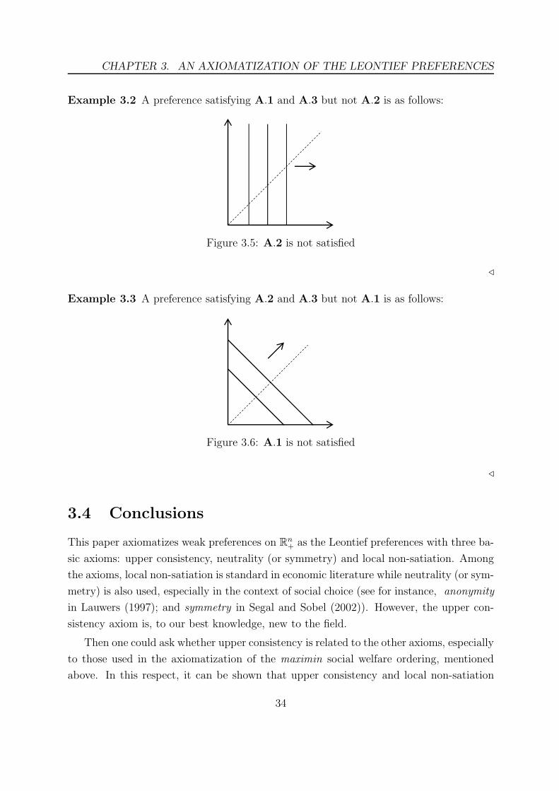
Example 3.2 A preference satisfying A.1 and A.3 but not A.2 is as follows:
Figure 3.5: A.2 is not satisfied
⊳
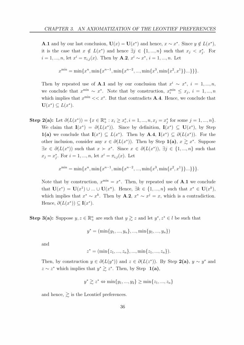
Example 3.3 A preference satisfying A.2 and A.3 but not A.1 is as follows:
Figure 3.6: A.1 is not satisfied
⊳
3.4 Conclusions
This paper axiomatizes weak preferences on Rn+ as the Leontief preferences with three ba-
sic axioms: upper consistency, neutrality (or symmetry) and local non-satiation. Among
the axioms, local non-satiation is standard in economic literature while neutrality (or sym-
metry) is also used, especially in the context of social choice (see for instance, anonymity
in Lauwers (1997); and symmetry in Segal and Sobel (2002)). However, the upper con-
sistency axiom is, to our best knowledge, new to the field.
Then one could ask whether upper consistency is related to the other axioms, especially
to those used in the axiomatization of the maximin social welfare ordering, mentioned
above. In this respect, it can be shown that upper consistency and local non-satiation
34

3.5. APPENDIX
together imply monotonicity (or weak Pareto) (see Lemma 3.2 in Appendix A). Also,
an example of preferences that satisfy upper consistency, but not Hammond equity can
be given (see Example 2 in Section 3.3), and it can easily be checked that the following
preferences satisfy Hammond equity but not upper consistency:
∀x ∈ R2+, u(x) = −max{x1, x2}.
3.5 Appendix
For x, y ∈ Rn+, we write x >> y if xi > yi for all i = 1, ..., n. We say that & on Rn
+ is
A.4: Monotonic if whenever x, y ∈ Rn+ are such that x >> y, we have x ≻ y.
Lemma 3.2 If & on Rn+ satisfies A.1 and A.3, then it satisfies A.4.
Proof. Consider y ∈ Rn+ such that x >> y. Then, min{x, y} = y and by A.1,
U(x) ⊆ U(y), which implies that x & y. Suppose x ∼ y and consider the following
n -dimensional box B(x, y) = {z ∈ Rn+ : xi ≥ zi ≥ yi, i = 1, ..., n}. Then, for any
z ∈ B(x, y), min{x, z} = z and min{z, y} = y and by A.1, x & z and z & y. Since x ∼ y,
we then conclude that x ∼ z ∼ y. But that contradicts A.3. Hence, x ≻ y. �
Theorem 3.3 Let & be a weak order on Rn+. Then,
(a) & satisfies A.1,A.2 and A.3 if and only if it is the Leontief preferences, and
(b) & satisfies A.1,A.2′ and A.3 if and only if it is an a-weighted Leontief preferences.
Proof. Since IF parts are easy to check, we prove ONLY IF parts. By Lemma 3.2 we
may assume that & satisfies A.4.
(a) Suppose & satisfies A.1−A.4. Consider x∗ ∈ l. Let
L(x∗) = {x ∈ Rn+ : xi ≥ x∗
i , i = 1, ..., n}.
We proceed in 3 steps.
Step 1(a): We claim thatU(x∗) = L(x∗). First, note that for any x ∈ L(x∗), min{x, x∗} =
x∗. Then by A.1, U(x) ⊆ U(x∗). In particular, x ∈ U(x∗). Hence, L(x∗) ⊆ U(x∗).
For the other inclusion, suppose ∃y ∈ U(x∗) such that y /∈ L(x∗). Since y ∈ U(x∗),
by transitivity of &, we conclude that U(y) ⊆ U(x∗). Consider x = min{y, x∗}. By
35
CHAPTER 3. AN AXIOMATIZATION OF THE LEONTIEF PREFERENCES
A.1 and by our last conclusion, U(x) = U(x∗) and hence, x ∼ x∗. Since y /∈ L(x∗),
it is the case that x /∈ L(x∗) and hence ∃j ∈ {1, ..., n} such that xj < x∗j . For
i = 1, ..., n, let xi = πi,j(x). Then by A.2, xi ∼ x∗, i = 1, ..., n. Let
xmin = min{xn,min{xn−1,min{xn−2, ...,min{x3,min{x2, x1}}...}}}.
Then by repeated use of A.1 and by our conclusion that xi ∼ x∗, i = 1, ..., n,
we conclude that xmin ∼ x∗. Note that by construction, xmini ≤ xj , i = 1, ..., n
which implies that xmin << x∗. But that contradicts A.4. Hence, we conclude that
U(x∗) ⊆ L(x∗).
Step 2(a): Let ∂(L(x∗)) = {x ∈ Rn+ : xi ≥ x∗
i , i = 1, ..., n, xj = x∗j for some j = 1, ..., n}.
We claim that I(x∗) = ∂(L(x∗)). Since by definition, I(x∗) ⊆ U(x∗), by Step
1(a) we conclude that I(x∗) ⊆ L(x∗). Then by A.4, I(x∗) ⊆ ∂(L(x∗)). For the
other inclusion, consider any x ∈ ∂(L(x∗)). Then by Step 1(a), x & x∗. Suppose
∃x ∈ ∂(L(x∗)) such that x ≻ x∗. Since x ∈ ∂(L(x∗)), ∃j ∈ {1, ..., n} such that
xj = x∗j . For i = 1, ..., n, let xi = πi,j(x). Let
xmin = min{xn,min{xn−1,min{xn−2, ...,min{x3,min{x2, x1}}...}}}.
Note that by construction, xmin = x∗. Then, by repeated use of A.1 we conclude
that U(x∗) = U(x1) ∪ ... ∪ U(xn). Hence, ∃k ∈ {1, ..., n} such that x∗ ∈ U(xk),
which implies that x∗ ∼ xk. Then by A.2, x∗ ∼ xj = x, which is a contradiction.
Hence, ∂(L(x∗)) ⊆ I(x∗).
Step 3(a): Suppose y, z ∈ Rn+ are such that y & z and let y∗, z∗ ∈ l be such that
y∗ = (min{y1, ..., yn}, ...,min{y1, ..., yn})
and
z∗ = (min{z1, ..., zn}, ...,min{z1, ..., zn}).
Then, by construction y ∈ ∂(L(y∗)) and z ∈ ∂(L(z∗)). By Step 2(a), y ∼ y∗ and
z ∼ z∗ which implies that y∗ & z∗. Then, by Step 1(a),
y∗ & z∗ ⇔ min{y1, ..., y2} ≥ min{z1, ..., zn}
and hence, & is the Leontief preferences.
36

3.5. APPENDIX
(b) Consider x∗ ∈ l(a1, ..., an). Note that ∀i, j = 1, ..., n,
(1
a1, ...,
1
an) ∗ πi,j(a1x
∗1, ..., anx
∗n) = x∗
i.e. the neutral (symmetric) image of x∗ is itself, since aix∗i = ajx
∗j ⇔ 1
aiajx
∗j = x∗
i . We
proceed in 3 steps.
Step 1(b): We claim that U(x∗) = L(x∗). First, by repeating the same argument as
in Step 1(a) we conclude that L(x∗) ⊆ U(x∗). For the other inclusion, suppose
∃y ∈ U(x∗) such that y /∈ L(x∗). Since y ∈ U(x∗), by transitivity of &, we conclude
that U(y) ⊆ U(x∗). Consider x = min{y, x∗}. By A.1 and by our last conclusion,
U(x) = U(x∗) and hence, x ∼ x∗. Since y /∈ L(x∗), x /∈ L(x∗) and ∃j ∈ {1, ..., n}
such that xj < x∗j . For i = 1, ..., n, let xi = ( 1
a1, ..., 1
an) ∗ πi,j(a1x1, ..., anxn). Then
by A.2′, xi ∼ x∗, i = 1, ..., n. Let
xmin = min{xn,min{xn−1,min{xn−2, ...,min{x3,min{x2, x1}}...}}}.
Then by repeated use of A.1 and by our conclusion that xi ∼ x∗, i = 1, ..., n, we
conclude that xmin ∼ x∗. Note that by construction, the i′th component of xi is
xii =
1aiajxj , for i = 1, ..., n. Then, xi
i < x∗i , for i = 1, ..., n since 1
aiajxj <
1aiajx
∗j =
1aiaix
∗i = x∗
i , which implies that xmin << x∗. But that contradicts A.4. Hence, we
conclude that U(x∗) ⊆ L(x∗).
Step 2(b): We claim that I(x∗) = ∂(L(x∗)). First, by repeating the same argument as
in Step 2(a) we conclude that I(x∗) ⊆ L(x∗). Then by A.4, I(x∗) ⊆ ∂(L(x∗)).
For the other inclusion, consider any x ∈ ∂(L(x∗)). Then by Step 1(b), x & x∗.
Suppose ∃x ∈ ∂(L(x∗)) such that x ≻ x∗. Since x ∈ ∂(L(x∗)), ∃j ∈ {1, ..., n} such
that xj = x∗j . For i = 1, ..., n, let xi = ( 1
a1, ..., 1
an) ∗ πi,j(a1x1, ..., anxn). Let
xmin = min{xn,min{xn−1,min{xn−2, ...,min{x3,min{x2, x1}}...}}}.
Note that by construction, ∀i = 1, ..., n, the i′th component of xi is xii =
1aiajxj =
1aiajx
∗j = 1
aiaix
∗i = x∗
i , and when i 6= j, ∀k ∈ {1, ..., n}\{i}, the i′th component of
xk is xki = xi ≥ x∗
i (recall that x ∈ ∂(L(x∗))), and when i = j, ∀k ∈ {1, ..., n}\{j},
the j′th component of xk is xkj = 1
ajakxk ≥ 1
ajakx
∗k = 1
ajajx
∗j = x∗
j . This implies that
xmin = x∗. Then, by repeated use of A.1 we conclude that
U(x∗) = U(x1) ∪ ... ∪U(xn).
37

CHAPTER 3. AN AXIOMATIZATION OF THE LEONTIEF PREFERENCES
Hence, ∃q ∈ {1, ..., n} such that x∗ ∈ U(xq), which implies that x∗ ∼ xq. Then by
A.2′, x∗ ∼ xj = x, which is a contradiction. Hence, ∂(L(x∗)) ⊆ I(x∗).
Step 3(b): Suppose y, z ∈ Rn+ are such that y & z and let y∗, z∗ ∈ l(a1, ..., an) be such
that
y∗ = (1
a1min{a1y1, ..., anyn}, ...,
1
anmin{a1y1, ..., anyn})
and
z∗ = (1
a1min{a1z1, ..., anzn}, ...,
1
anmin{a1z1, ..., anzn}).
Then, by construction y ∈ ∂(L(y∗)) and z ∈ ∂(L(z∗)). By Step 2(b), y ∼ y∗ and
z ∼ z∗ which implies that y∗ & z∗. Then, by Step 1(b),
y∗ & z∗ ⇔ min{a1y1, ..., anyn} ≥ min{a1z1, ..., anzn}
and hence, & is an a-weighted Leontief preferences.
�
38

Bibliography
[1] Bosmans, K., and E. Ooghe (2006). ”A Characterization of Maximin.” Mimeo,
Katholieke Universiteit Leuven.
[2] Chambers, C.P. (2009). ”Intergenerational Equity: Sup, Inf, Lim Sup, and Lim Inf.”
Social Choice and Welfare 39, 243-252.
[3] Dorfman, R. (2008). ”Wassily Leontief (1906-1999).” In: The New Palgrave Dictio-
nary of Economics, 2nd ed. Eds. S.N. Durlauf and L.E. Blume. New York: Palgrave
Macmillan.
[4] Dorfman, R., Samuelson, P.A., and R.M. Solow (1958). Linear Programming and
Economic Analysis. New York: McGraw-Hill.
[5] Kreps, D.M. (1988). Notes on the Theory of Choice. Colorado: Westview Press.
[6] Lauwers, L. (1997). ”Rawlsian Equity and Generalized Utilitarianism with Infinite
Population.” Economic Theory 9, 143-150.
[7] Leontief, W. (1951). The Structure of American Economy, 1919-1939, 2nd ed. New
York: Oxford University Press.
[8] Miyagishima, K. (2010). ”A Characterization of Maximin Social Ordering.” Economics
Bulletin 30, 1278-1282.
[9] Segal, U., and J. Sobel (2002). ”Min, Max, and Sum.” Journal of Economic Theory
106, 126-150.
39


Chapter 4
Remarks on Young’s Theorem 1
Abstract: In this paper we analyze the simple case of voting over two alternatives with
variable electorate. Our main findings are (a) the axiom of continuity is redundant in the
axiomatization of scoring rules in Young (1975), SIAM J. Appl. Math. 28: 824-838, (b)
the smaller set of axioms characterize the scoring rules when indifferences are allowed in
voter’s preferences, (c) a version of May’s theorem can be derived from this last result
and finally, (d) in each of these results, the axioms of neutrality and cancellation can be
used interchangeably.
JEL: D71, D72
Keywords: Scoring rules, Young’s theorem, May’s theorem
4.1 Introduction
In this paper we reconsider the problem of axiomatizing scoring rules. Early results on this
problem are due to Smith (1973) and Young (1975). They characterized social welfare and
social choice functions, respectively, as scoring rules with four basic axioms: anonymity,
neutrality, consistency (or separability, or reinforcement) and continuity (or Archimedian,
or overwhelming majority). Following them, Myerson (1995) showed that essentially the
same set of axioms characterize scoring rules even if some of the assumptions of Smith
(1973) and Young (1975) are weakened.
Our objective in this paper is to point out an important detail that has seemingly been
ignored in this literature: in the special case of two alternatives, the continuity axiom in
1Published in Economics Bulletin, 2012, 32 (1): 706-714. I am thankful to the associate editor JordiMasso and two anonymous referees for their helpful comments.
41

CHAPTER 4. REMARKS ON YOUNG’S THEOREM
Young (1975) is redundant in the axiomatization of scoring rules. Hence, our main result
is (Theorem 4.3 in Section 4.3.1) ”When there are two alternatives, a social choice function
is anonymous, neutral and consistent if and only if it is a simple scoring function.” We also
show that the same result holds, i.e. the smaller set of axioms characterize this voting
rule, when indifferences are allowed in the voters’ preferences (Theorem 4.5 in Section
4.3.2). Moreover, from this result we derive another result (Theorem 4.6 in Section 4.3.2)
that can be seen as a variant of May’s theorem in May (1952), and hence establish a
formal connection between the two classic results, Young’s Theorem and May’s Theorem.
Finally, we also show that in each of our results, axioms of neutrality and cancellation
property can be used interchangeably (Proposition 4.4 and 4.7).
In the next section we introduce our notation and the main definitions. Section 4.3
gives the main results and the last section concludes.
4.2 The preliminaries
Let Rn denote the set of all n-tuples of real numbers and let Rn+ be its nonnegative orthant.
The notions of weak (and associated indifference relation) and strict preferences over a
set B are defined as usual and when a ∈ B is weakly, strictly preferred and indifferent to
b ∈ B, we write a & b, a ≻ b and a ∼ b, respectively. A transposition on set B = {a, b},
that is a permutation that exchanges the roles of a and b, is denoted as a ⇆ b.
Our main setting follows closely that of Young (1975). Let A = {a1, ..., am} be the set
of alternatives. Let N denote the set of nonnegative integers which constitute names for
the voters and let P be the set of all preference orders (strict) on A. For any finite V ⊂ N,
a profile is a function from V to P and a social choice function (SCF) is a function from
set X of all profiles to the family of non-empty subsets of A, 2A\{∅}. A SCF is said to
be anonymous if it depends only on the number of voters associated with each preference
order. We can represent the domain of an anonymous SCF by Nm!, i.e. the set of all
m!-tuples with nonnegative integer coordinates, indexed by P, where for any x ∈ Nm! and
any p ∈ P, xp represents the number of voters having preference order p. Let Sm be the
group of permutations of the index set {1, 2, ..., m}. Each σ ∈ Sm induces permutations
of the alternatives (which we also denote by σ), and hence profiles, in the natural way.
We say that SCF is neutral if f ◦ σ = σ ◦ f for all σ ∈ Sm. An anonymous SCF f is
consistent if ∀x′, x′′ ∈ Nm! such that f(x′) ∩ f(x′′) 6= ∅, f(x′ + x′′) = f(x′) ∩ f(x′′), and
it is continuous if whenever f(x) = {ai}, ∀y ∈ Nm! there is a sufficiently large integer n
such that f(y + n′x) = {ai} for n′ ≥ n.
42
4.3. THE AXIOMS FOR SCORING RULES WHEN M = 2
We say that a SCF f has the cancellation property if whenever x is a profile such that
the number of voters preferring ai to aj equals that of preferring aj to ai for all pairs
ai 6= aj, then f(x) = A. A SCF is a simple scoring function, denoted by f s, if there is a
vector s = (s1, ..., sm) ∈ Rm of scores such that for any given profile, it assigns a score of
si to each voter’s i′th most preferred alternative and chooses the alternative(s) with the
highest total score at that profile.2 A SCF is trivial (f ∗) if ∀x ∈ Nm!, f ∗(x) = A. Note
that f ∗ is a simple scoring function with s = (0, ..., 0).
The following result is known as Young’s Theorem (Theorem 1.(ii) in Young, 1975):
Theorem 4.1 Let f be a SCF. Then, f is anonymous, neutral, consistent and continuous
if and only if it is a simple scoring function.
4.3 The axioms for scoring rules when m = 2
4.3.1 Two remarks on Young’s theorem
Before we consider the case of m = 2, we prove the following Lemma which holds for any
finite m.
Lemma 4.2 Suppose f is an anonymous, neutral and consistent SCF. Then,
(a) f is either trivial or it contains all the singletons of 2A\{∅} in its range:
∀ai ∈ A, ∃x ∈ Nm! such that f(x) = {ai}.
(b) Let e = (1, ..., 1) ∈ Nm!. Then, ∀n ∈ N, f(ne) = A.
Proof. (a) Note that when m = 1 the result is trivial. Suppose m ≥ 2. We show
that R(f), the range of f , includes at least one singleton {ai}. Then, the result follows
by neutrality. When m = 2, the claim is trivial since f 6= f ∗ immediately implies that
∃x ∈ N2! such that f(x) = {ai} for some ai ∈ {a1, a2}. Let m ≥ 3 and suppose R(f)
does not contain any singleton. Then, we claim that it can’t have any 2-element sets,
3 -element sets,..., (m − 1)-element sets. Because if R(f) has a 2-element set {ai, aj},
then by neutrality it has another 2-element set {ai, ak}. Then for x′ ∈ f−1({ai, aj}) and
x′′ ∈ f−1({ai, ak}), consistency implies that f(x′+x′′) = {ai}, which is a singleton. Hence,
we reach to a contradiction. Similarly, we conclude that R(f) can’t have any k-element
sets, for 3 ≤ k < m. But then, f = f ∗.
2Note that scoring rules constitute rather general class of voting procedures. In particular, the possi-bility of assigning lower scores to more preferred alternatives is allowed.
43

CHAPTER 4. REMARKS ON YOUNG’S THEOREM
(b) We show that f(e) = A. Then the result follows by consistency. Note that e ∈ Nm!
is invariant under all permutations in Sm. Then f(e) must be so by neutrality. But in
2A\{∅}, the only set with that property is A. �
We remark here that Lemma 4.2 (b) is already established in Young (1975). Let us
now consider the case of m = 2. Our main result is the following:
Theorem 4.3 Let m = 2 and let f be a SCF. Then, f is anonymous, neutral and
consistent if and only if it is a simple scoring function.
Proof. Since the IF part is easy to verify we prove the ONLY IF part. For any x =
(x1, x2) ∈ N2 ⊂ R2+, let x1 be the number of voters with preference p1 : a1 ≻ a2 and let
x2 be that with p2 : a2 ≻ a1. We shall partition N2 ⊂ R2+ as follows:
D = {x ∈ N2 : x1 = x2};
D′ = {x ∈ N2 : x1 > x2};
D′′ = {x ∈ N2 : x1 < x2}.
Then by Lemma 4.2 (b), ∀x ∈ D, f(x) = {a1, a2}. We claim that ∀x′ ∈ D′, f(x′) = f(1, 0).
Suppose ∃x′ ∈ D′ such that f(x′) = f(1, 0). Then, by consistency
f(x′ + (1, 0)) = f(x′1 + 1, x′
2) = f(1, 0)
and
f(x′ + (1, 1)) = f(x′1 + 1, x′
2 + 1) = f(1, 0).
Hence, for any such x′ ∈ D′, its two immediate neighbors, one on the right side and one
on the upper right side, take the same value. Since (1, 0) ∈ D′, this proves our claim. By
neutrality, then ∀x′′
∈ D′′
, f(x′′
) = f(0, 1). Then by Lemma 4.2 (a), f is either f ∗, or f1:
f1(x) =
A if x ∈ D
{a1} if x ∈ D′
{a2} if x ∈ D′′
,
or f2:
f2(x) =
A if x ∈ D
{a2} if x ∈ D′
{a1} if x ∈ D′′
.
44

4.3. THE AXIOMS FOR SCORING RULES WHEN M = 2
Since f1 and f2 correspond to f s with s1 > s2 and s1 < s2 respectively, the proof is
completed. �
Let us show that one can use the axioms of neutrality and cancellation property
interchangeably in Theorem 4.3.
Proposition 4.4 Let m = 2 and let f be an anonymous and consistent SCF. Then, f
has cancellation property if and only if it is neutral.
Proof. IF: We have shown in Lemma 4.2 (b) that anonymity, consistency and neutrality
imply that, ∀x ∈ D, f(x) = {a1, a2}. Since m = 2, any profile x ∈ N2 is such that the
number of voters who prefers a1 ≻ a2 is same as that of who prefers a2 ≻ a1, if and only
if x ∈ D. Hence, f satisfies the cancellation property.
ONLY IF: Suppose f satisfies anonymity, consistency and cancellation property, but
not neutrality: ∃y ∈ N2 such that f◦σ′(y) 6= σ′◦f(y) for some σ′ ∈ S2. The only candidate
for such σ′ ∈ S2 is σ′ : a1 ⇆ a2. Note that if one of f ◦σ′(y) ∈ 2A\{∅} and f(y) ∈ 2A\{∅}
is A, then consistency implies that they both must be A, since σ′(y)+ y ∈ D and by can-
cellation property, f(σ′(y)+y) = A. But then f ◦σ′(y) = σ′ ◦f(y) = A which contradicts
to our assumption. Hence, none of f ◦ σ′(y) ∈ 2A\{∅} and f(y) ∈ 2A\{∅} is A. Suppose
f ◦σ′(y) = {ai} and f(y) = {aj} for i, j ∈ {1, 2}, i 6= j. Then f ◦σ′(y) = σ′ ◦ f(y) = {ai},
which is a contradiction. Hence, the only possibility left is f ◦ σ′(y) = f(y) = {ai} for
some i ∈ {1, 2}. Then by consistency f(σ′(y) + y) = {ai}, which contradicts to cancella-
tion property. This completes our proof. �
In our opinion, redundancy of the continuity axiom in Theorem 4.1 when m = 2 is
not so obvious until one proves Theorem 4.3. However, one can also verify it directly
from Theorem 1.(i) in Young (1975) which states that a SCF is anonymous, neutral and
consistent if and only if it is a (composite) scoring function. Provided that Theorem 1.(i)
is proven, it suffices to notice that when m = 2, a composition g = f s2 ◦ f s1 of two
simple scoring functions f s1, f s2, defined as g(x) = f s1(x) if f s1(x) ⊆ A is a singleton set,
otherwise apply f s2 to break the ties in f s1(x), is a simple scoring function. Note that
there are two possibilities: either f s1 is trivial or it is not. Suppose f s1 = f ∗. Then, since
g = f s2 ◦ f ∗ = f s2, g is a simple scoring function. Now suppose f s1 6= f ∗. Then, since
when m = 2, f s1(x) produces ties if and only if x ∈ D and since f s2(x) = A for x ∈ D,
we conclude that g = f s1, hence g is a simple scoring function.
45

CHAPTER 4. REMARKS ON YOUNG’S THEOREM
4.3.2 Allowing for indifferences in voters’ preferences
Let us now change our initial setting by allowing indifferences in the individual’s pref-
erences, hence enlarging the domain of SCF. Sets A, Sm and N are defined as above in
Section 4.2. Let W be the set off all weak preference orders on A. For any finite V ⊂ N, an
extended profile is a function from V to W and an extended social choice function (ESCF)
is a function from set Y of all extended profiles to the set 2A\{∅}. An ESCF is said to
be anonymous if it depends only on the number of voters associated with each preference
order. We can represent the domain of an anonymous ESCF by N#W. The notions of
neutrality, consistency and cancellation property for an ESCF are defined analogously to
that for a SCF.
Since scoring rules are initially defined for profiles with strict preferences in Section
4.2, it needs to be generalized. As we are eventually interested in the case of m = 2, we
impose a rather weak condition in our generalization: whenever alternatives are indifferent
to each others at a given preference they must receive the same score (for a more specific
generalization which applies to the case of any finite m, see Vorsatz, 2008). So when
m = 2, an ESCF is a simple scoring function, denoted by F s, if there is a vector s =
(s1, s2, s3) ∈ R3 of scores such that for any given profile, it assigns a score of si to each
voter’s i′th strictly most preferred alternative, for i = 1, 2, and assigns a score of s3 to
each voter’s indifferent alternatives, and chooses the alternative(s) with the highest total
score at that profile. An ESCF is trivial (F ∗) if ∀x ∈ N#W, F ∗(x) = A. Note that when
m = 2, F ∗ is a simple scoring function with s = (0, 0, 0).
Theorem 4.5 Let m = 2 and let F be an ESCF. Then, F is anonymous, neutral and
consistent if and only if it is a simple scoring function.
Proof. IF: F s is clearly anonymous since the outcome of F s depends only on the total
scores and that in turn depends only on the number of voters associated with each pref-
erence. F s is neutral since exchanging the roles of a1 and a2 is same as exchanging the
total scores received by each. F s is consistent since the total score received by ai under
x + y ∈ N3 is the sum of the scores received under each of x, y ∈ N3, for any x, y ∈ N3
and i = 1, 2.
ONLY IF: For any x = (x1, x2, x3) ∈ N3 ⊂ R3+, let x1, x2 and x3 be the number of
voters with the preferences p1 : a1 ≻ a2, p2 : a2 ≻ a1 and p3 : a1 ∼ a2, respectively. We
46

4.3. THE AXIOMS FOR SCORING RULES WHEN M = 2
shall partition N3 ⊂ R3+ as follows:
D3 = {x ∈ N3 : x1 = x2, x3 ∈ N};
D′3 = {x ∈ N3 : x1 > x2, x3 ∈ N};
D′′3 = {x ∈ N3 : x1 < x2, x3 ∈ N}.
Firstly, note that ∀x ∈ D3, F (x) = {a1, a2} since x ∈ D3 is invariant under all permuta-
tions in S2 (recall that the indifference relation is symmetric) and by neutrality so must
be F (x). But the only set with that property in {a1}, {a2} and {a1, a2} is the very last
one.
Let Pn ⊂ N3 be defined as follows: ∀n ∈ N,Pn = {x ∈ N3 : x1, x2 ∈ N, x3 = n}.
We claim that for n ≥ 1, if F (x) = F (1, 0, 0), ∀x ∈ Pn−1 ∩ D′3, then F (x) = F (1, 0, 0),
∀x ∈ Pn ∩ D′3. Suppose y ∈ Pn−1 ∩ D′
3 and F (y) = F (1, 0, 0). Then by consistency,
F (y + (0, 0, 1)) = F (y) = F (1, 0, 0) since (0, 0, 1) ∈ D3 and F (0, 0, 1) = A. But for
n ≥ 1, Pn = {x ∈ N3 : x = y + (0, 0, 1), y ∈ Pn−1} and this proves our claim.
Recall that we already showed in the proof of Theorem 4.3 that F (x) = F (1, 0, 0),
∀x ∈ P0∩D′3. Hence, we conclude that ∀x ∈ D′
3, F (x) = F (1, 0, 0), and then by neutrality,
∀x ∈ D′′3 , F (x) = F (0, 1, 0). To complete the proof, suppose F 6= F ∗, then F includes all
singletons in its range since F 6= F ∗ implies that ∃x ∈ N3 such that F (x) = {ai} for some
ai ∈ A and hence by neutrality, ∃xi ∈ N3 such that F (xi) = {ai}, for i = 1, 2. Combining
our last observation with the above conclusions, we have established that F is either F ∗,
or F1 :
F1(x) =
A if x ∈ D3
{a1} if x ∈ D′3
{a2} if x ∈ D′′
3
,
or F2 :
F2(x) =
A if x ∈ D3
{a2} if x ∈ D′3
{a1} if x ∈ D′′
3
.
Since F1 and F2 correspond to F s with s1 > s2 and s1 < s2 respectively, the proof is
completed. �
Let us now derive a variant of May’s theorem from Theorem 4.5 above. First, we
need to introduce some more properties for anonymous ESCFs. For any extended profile
x ∈ N3, let N(ai, x) ∈ N be the number of voters who prefers (weakly) ai to aj at x ∈ N3,
47

CHAPTER 4. REMARKS ON YOUNG’S THEOREM
for i, j ∈ {1, 2} and i 6= j. An anonymous ESCF is a simple majority rule (FM) if
FM(x) =
{
{ai} if N(ai, x) > N(aj , x)
{a1, a2} if N(ai, x) = N(aj , x)
for i, j ∈ {1, 2}, i 6= j. It is an inverse simple majority rule (F−M) if
F−M(x) =
{
{ai} if N(ai, x) < N(aj , x)
{a1, a2} if N(ai, x) = N(aj , x)
for i, j ∈ {1, 2}, i 6= j. Finally, anonymous ESCF is positive responsive to voter addition
(positive responsiveness) if whenever ai ∈ F (x) for x ∈ N3, and y ∈ N3 is obtained from
x ∈ N3 by adding one more voter with preferences of ai ≻ aj, we have F (y) = {ai}, for
i, j ∈ {1, 2}, i 6= j. The second part of the following result is a variant of May’s Theorem
(May (1952)):
Theorem 4.6 Let m = 2 and let F be an ESCF. Then,
(a) F is anonymous, neutral and consistent if and only if it is either trivial, or a simple
majority rule, or an inverse majority rule and
(b) F is anonymous, neutral and positive responsive if and only if it is a simple majority
rule.
Proof. Since the IF parts are easy we prove the ONLY IF parts.
(a) By definition, F1 and F2 in the proof of Theorem 4.5 correspond to simple majority
rule and inverse simple majority rule, respectively.
(b) We present two proofs.
1. Let us show that positive responsiveness with anonymity and neutrality imply
consistency. From the proof of Theorem 4.5, we know that anonymity and neutrality
imply that, ∀x ∈ D3, F (x) = {a1, a2}. For any x = (x1, x2, x3) ∈ N3, let xD3 ∈ D3 be
defined as xD3 = (min{x1, x2},min{x1, x2}, x3). We can write x as x = xD3 + (x− xD3).
We claim that F (x) = F (x − xD3). Note that if x ∈ D3, then F (x) = F (0) = A, hence
the claim is true. Suppose x /∈ D3. Then one can generate x ∈ N3 from xD3 ∈ D3 and
x−xD3 ∈ N3 from 0 ∈ D3 by one and the same procedure: if x1 > x2, adding |x1 − x2| > 0
voters, one at a time, who strictly prefers a1 to a2, if otherwise adding the same number of
voters with the reverse preferences. Then, by positive responsiveness, F (x) = F (x−xD3)
as we claimed, and moreover, F (x) = A if and only if x = xD3 ∈ D3.
48
4.3. THE AXIOMS FOR SCORING RULES WHEN M = 2
Suppose x, y ∈ N3 are such that F (x) ∩ F (y) 6= ∅. We can express as F (x) ∩ F (y) =
F (x − xD3) ∩ F (y − yD3). Let z = x + y and notice that zD3 = xD3 + yD3 , since the
’min’ operator is additive. Hence, F (z) = F (xD3 + yD3 + (x − xD3) + (y − yD3)) =
F ((x−xD3)+(y−yD3)). We claim that F ((x−xD3)+(y−yD3)) = F (x−xD3)∩F (y−yD3).
Notice that if at least one of x, y is in D3, then the claim is established: if x ∈ D3, then
x = xD3 and F (x − xD3) = A. Suppose x, y /∈ D3. Then, F (x − xD3) ∩ F (y − yD3) 6= ∅
implies F (x− xD3) = F (y − yD3) = {ai} for some i ∈ {1, 2}. By positive responsiveness,
that is only possible if min{x1, x2} = xj and min{y1, y2} = yj for j ∈ {1, 2} and j 6= i.
Then by positive responsiveness, F ((x− xD3) + (y − yD3)) = {ai} since one can generate
(x− xD3) + (y − yD3) ∈ N3 from 0 ∈ D3 by adding (xi − xj) + (yi − yj) many voters with
strict preferences of ai ≻ aj. Hence, our second claim is established, which then implies
that F is consistent.
Then, the result in part (a) implies that F is one of F ∗, F1 and F2. But none of F ∗
and F2 satisfies positive responsiveness. Hence, F = F1 which is the simple majority rule.
2. The proof above is rather indirect and a more direct proof is as follows. We know
that anonymity and neutrality imply that, ∀x ∈ D3, F (x) = {a1, a2}. We claim that
∀x′ ∈ D′3, F (x′) = {a1}. Suppose x′ = (x′
1, x′2, x
′3) ∈ D′
3. Consider x∗ = (x′
2, x′2, x
′3) ∈ D3.
Then, F (x∗) = {a1, a2}. We can generate x′ from x∗ by adding (x′1 − x′
2) voters, one at
a time, with the preferences of a1 ≻ a2. Then by positive responsiveness, F (x′) = {a1}.
Hence, ∀x′ ∈ D′3, F (x′) = {a1} and by neutrality, ∀x
′′
∈ D′′
3 , F (x′′
) = {a2}, which imply
that F = F1, which is the simple majority rule. �
May (1952) axiomatizes majority rule with anonymity, neutrality and strong mono-
tonicity. The main difference between May’s Theorem and Theorem 4.6 (b) is, May (1952)
considers a fixed electorate setting while we consider a variable electorate setting. Then,
the axiom of positive responsiveness to voter addition should be seen as a modification of
the strong monotonicity axiom to the new setting.3
Let us show that one can use cancellation property axiom instead of neutrality in
Theorem 4.5 and 4.6.
Proposition 4.7 Let m = 2 and let F be an anonymous ESCF. Then,
(a) If F is consistent then it has cancellation property if and only if it is neutral, and
3Strictly speaking, positive responsiveness to voter addition can not be stated in the original settingwith fixed electorate. But it captures the underlying idea of the strong monotonicity axiom, and henceTheorem 4.6 (b) can be seen as a variant of May’s Theorem.
49

CHAPTER 4. REMARKS ON YOUNG’S THEOREM
(b) If F has cancellation property and is positive responsive then it is consistent.
Proof. (a) IF: We have shown in the proof of Theorem 4.5 that anonymity, consistency
and neutrality imply that, ∀x ∈ D3, F (x) = A. Since m = 2, any profile x ∈ N3 is such
that the number of voters who prefers a1 & a2 is same as that of who prefers a2 & a1, if
and only if x ∈ D3. Hence, F satisfies the cancellation property.
ONLY IF: Let F|P0be restriction of F into P0 = {x ∈ N3 : x1, x2 ∈ N, x3 = 0} ⊂ N3.
Note that F|P0 is a SCF and since F satisfies anonymity, consistency and cancellation
property, so is F|P0. Then by Proposition 4.4, we conclude that F|P0
satisfies neutrality.
Note also that by cancellation property, F (0, 0, 1) = A, which implies that F (0, 0, x3) = A
for all x3 ≥ 1, by consistency. Then, we conclude that ∀x = (x1, x2, x3) ∈ N3 such that
x3 ≥ 1, F (x1, x2, x3) = F (x1, x2, 0) = F|P0(x1, x2) since F (x1, x2, x3) = F (x1, x2, 0) +
F (0, 0, x3) = F (x1, x2, 0), where the last equality follows by consistency. Then, ∀x ∈
N3, ∀σ ∈ S2, F ◦ σ(x) = F|P0 ◦ σ(x) = σ ◦ F|P0(x1, x2) = σ ◦ F (x) since the first and the
last equality follows by our second conclusion, while the second equality follows by our
first conclusion, and hence F is neutral.
(b) We prove the statement indirectly showing that anonymity, cancellation prop-
erty and positive responsiveness imply that F = FM . By definition, cancellation prop-
erty implies that ∀x ∈ D3, F (x) = {a1, a2}. Repeating the same argument as above
in the second proof of Theorem 4.6 (b), we conclude that, by positive responsiveness,
∀x′ ∈ D′3, F (x′) = {a1}. Let x
′′
= (x′′
1 , x′′
2 , x′′
3) ∈ D′′
3 . Consider x∗ = (x′′
1 , x′′
1 , x′′
3) ∈ D3.
Then, F (x∗) = {a1, a2}. We can generate x′′
from x∗ by adding (x′′
2 − x′′
1) voters, one at
a time, with the preferences of a2 ≻ a1. Then by positive responsiveness, F (x′′
) = {a2}.
Hence ∀x′′
∈ D′′
3 , F (x′′
) = {a2}. So, F = FM and hence, it is consistent. �
4.4 Final comments
When it is presented Young’s Theorem is often accompanied by the following remark: ”its
proof is difficult and omitted” (see for instance, Chap. 9 in Moulin, 1988). However, the
analysis above shows that in the special case of voting over two alternatives it can easily
be proved. One may also wonder whether the axiom of continuity can be eliminated when
there are more than two alternatives. The answer to this question is negative since the
example of a (composite) scoring function satisfying the axioms of anonymity, neutrality
and consistency but not continuity, given in Section 3 of Young (1975), can easily be
extended to the case of any finite (but three or more) alternatives. This observation
50

4.4. FINAL COMMENTS
implies that any such elimination contradicts Theorem 1 in Young (1975).
It may seem that the setting with two alternatives is rather restrictive, especially in
the context of scoring rules. However, note that the analysis of this simple case can
shed a light on possible improvements of some of the axiomatization results in voting
theory. For instance, as majority rule and approval voting (AV) coincide when m = 2,
the result in Theorem 4.6 (a) is related to the axiomatization of AV in Fishburn (1978).
In the simple case it is easy to see that the axioms of neutrality and cancellation can
be used interchangeably (see Proposition 4.7). On the other hand, Alos-Ferrer (2006)
shows that one can drop neutrality in the presence of anonymity, consistency, cancellation
and faithfulness in Fishburn (1978)’s axiomatization of AV. Hence, Alos-Ferrer (2006)’s
result can be seen as an extension of Theorem 4.6 (a). Finally, note also that Theorem
4.6 (a) admits another extension: one can keep neutrality and drop cancellation in the
axiomatization of AV, which is, to my best knowledge, an open question.
51


Bibliography
[1] Alos-Ferrer, C. (2006) ”A simple characterization of approval voting” Social Choice
and Welfare 27, 621-625.
[2] Fishburn, P.C. (1978) ”Symmetric and consistent aggregation with dichotomous vot-
ing” in Aggregation and Revelation of Preferences by J-J. Laffont, Eds., North Hol-
land: Amsterdam.
[3] May, K.O. (1952) ”A set of independent and sufficient conditions for simple majority
decision” Econometrica 20, 680-684.
[4] Moulin, H. (1988) Axioms of Cooperative Decision Making, Cambridge University
Press: Cambridge.
[5] Myerson, R.B. (1995) ”Axiomatic derivation of scoring rules without the ordering
assumption” Social Choice Welfare 12, 59-74.
[6] Smith, J.H. (1973) ”Aggregation of preferences with variable electorate” Economet-
rica 41, 1027-1041.
[7] Vorsatz, M. (2008) ”Scoring rules on dichotomous preferences” Social Choice Welfare
31, 151-162.
[8] Young, H.P. (1975) ”Social choice scoring functions” SIAM J. Appl. Math. 28, 824-
838.
53


Chapter 5
Approval Voting without
Faithfulness
Abstract: In this short note, we analyze the implications of dropping the axiom of
faithfulness in the axiomatization of Approval Voting, due to P.C. Fishburn. We show that
a ballot aggregation function satisfies the remaining axioms (neutrality, consistency and
cancellation) if and only if it is either a function that chooses the whole set of alternatives,
or an Approval Voting, or a function that chooses the least approved alternatives.
JEL: D71, D72
Keywords: Approval voting, Faithfulness, Inverse approval voting
5.1 Introduction
There are a number studies related to axiomatization of Approval Voting (AV) in the
literature (for a survey, see Hu, 2010). Early results on this problem are due to Fishburn
(1978a, 1978b). Fishburn (1978a) shows that AV is the only ballot aggregation function
(BAF) satisfying the axioms of neutrality, consistency, cancellation and faithfulness, while
Fishburn (1978b) axiomatizes AV with the axioms of neutrality, consistency and disjoint
equality. Alos-Ferrer (2006) shows that one can drop the axiom of neutrality in the
axiomatization of Fishburn (1978a).
The primary objective of this short paper is to investigate the implications of dropping
the axiom of faithfulness in the axiomatization of Fishburn (1978a), hence to analyze
cutting power of this axiom. Our main finding is (Theorem 5.1 in Section 5.2), a BAF
satisfies the axioms of neutrality, consistency and cancellation if and only if it is either
55

CHAPTER 5. APPROVAL VOTING WITHOUT FAITHFULNESS
a trivial function that chooses the whole set of alternatives at all profiles, or AV, or its
inverse, that is a function that chooses the least approved alternatives.
5.2 Characterization
Let N denote the set of nonnegative integers. Let X be a (finite) set of alternatives and
let S be the set of all permutations of X . For σ ∈ S and Y ⊆ X , σ(Y ) ⊆ X is the image
of Y under σ. A ballot B is a nonempty subset of X and let B = 2X\{∅} be the set of
all admissible ballots. Voters can cast any ballot, approving as many candidates as they
want. A voter response profile is a function π : B→ N such that π(B) is the number of
voters who cast ballot B. Let Π be the set of all possible voter response profiles, including
the empty profile π0 with π0(B) = 0 for all B ∈ B. A ballot aggregation function (BAF)
is a correspondence f which assigns to every possible voter response profile π ∈ Π, a
nonempty set of selected alternatives, ∅ ( f(π) ⊆ X . A BAF is an approval voting (fA )
if
fA(π) = argmax∑
x∈X
{π(B) : x ∈ B ∈ B},
it is an inverse approval voting (f−A) if
f−A(π) = argmin∑
x∈X
{π(B) : x ∈ B ∈ B},
and it is a trivial function (f ∗) if f ∗(π) = X, ∀π ∈ Π.
Given x ∈ X and π ∈ Π, the number of voters who approve of x in π is given by
v(x, π) =∑
{π(B) : x ∈ B ∈ B}.
For any B ∈ B, let πB ∈ Π denote the voter response profile with πB(B) = 1 and
πB(B′) = 0 for all B′ 6= B, i.e. πB consists of only one ballot B. When B ∈ B consists of
a single element x ∈ X , we write πx instead of π{x}. For any π, π′ ∈ Π, π + π′ ∈ Π is a
voter response profile with (π + π′)(B) = π(B) + π′(B), ∀B ∈ B, and whenever π, π′ ∈ Π
are such that π(B) = π′(B),∀B ∈ B, we write π = π′.
A BAF satisfies
Neutrality: if f(π ◦ σ) = σ(f(π)) for every σ ∈ S and for every π ∈ Π, where π ◦ σ ∈ Π
is defined as (π ◦ σ)(B) = π(σ(B)), ∀B ∈ B;
Faithfulness: if f(πB) = B for all B ∈ B;
56

5.2. CHARACTERIZATION
Consistency: if whenever f(π)∩f(π′) 6= ∅ for π, π′ ∈ Π, we have f(π+π′) = f(π)∩f(π′);
Cancellation: if whenever π ∈ Π satisfies v(x, π) = v(y, π) for all x, y ∈ X , then f(π) =
X .
For interpretations of the axioms, see Fishburn (1978a,b) and Hu (2010). We now
state and prove our main result (of which part (b) is already established in Fishburn
(1978a)):
Theorem 5.1 Let f be a BAF. Then
(a) f satisfies neutrality, consistency and cancellation if and only if it is either a trivial
function, or an approval voting, or an inverse approval voting, and
(b) in addition, such f is faithful if and only if it is an approval voting.
Proof. Since the IF parts are easy to prove, we prove the ONLY IF parts.
(a) We proceed in 4 steps. We remark here that Steps 2, 3 in our proof are the same
as Steps 1, 2 in the proof of Theorem 1 in Alos-Ferrer (2006).
Step 1: Let us prove that for all B ⊆ X , f(πB) is either B, or X\B or X , and similarly,
f(∑
x∈B
πx) is either B, or X\B or X . To see this, note that both πB ∈ Π and∑
x∈B
πx ∈ Π are invariant under any permutation σB ∈ S that permutes the elements
of B and X\B in an arbitrary way, but does not interchange the elements of these
two sets. That is, for any such σB ∈ S,
πB ◦ σB = πB
and
(∑
x∈B
πx) ◦ σB =∑
x∈B
πx.
Then, by neutrality so must be f(πB) and f(∑
x∈B
πx): for any such σB ∈ S,
σB(f(πB)) = f(πB)
and
σB(f(∑
x∈B
πx)) = f(∑
x∈B
πx).
But it is easy to check that the only sets in 2X\{∅} with such property (invariant
under any σB ∈ S) are B, X\B and X .
57

CHAPTER 5. APPROVAL VOTING WITHOUT FAITHFULNESS
Step 2: Let us prove that for all π ∈ Π and for all B′, B′′ ⊆ X such that B′ ∩ B′′ = ∅,
we have
f(π + πB′∪B′′) = f(π + πB′ + πB′′).
To see this, note that cancellation implies that
f(πB′ + πB′′ + πX\(B′∪B′′)) = X.
Then, by consistency,
f(π + πB′∪B′′) = f(π + πB′∪B′′ + πB′ + πB′′ + πX\(B′∪B′′)).
Note also that by cancellation,
f(πB′∪B′′ + πX\(B′∪B′′)) = X
and then by consistency,
f(π + πB′ + πB′′) = f(π + πB′ + πB′′ + πB′∪B′′ + πX\(B′∪B′′)).
Hence,
f(π + πB′∪B′′) = f(π + πB′ + πB′′). [1]
Step 3: Let π ∈ Π be an arbitrary voter response profile. Let π′ ∈ Π be such that
v(x, π) = v(x, π′) for all x ∈ X , but π′ consists only of singleton ballots, i.e. π′(B) >
0 implies that |B| = 1. The profile π′ is constructed from π by taking apart each
ballot cast under π into separate, singleton ballots. Then iteration of [1], starting
from π0 ∈ Π, shows that f(π) = f(π′).
Step 4: Let x ∈ X be any alternative and consider πx ∈ Π. By Step 1, f(πx) is either
{x}, or X\{x}, or X . We show that these possibilities correspond, respectively, to
the cases of f being either fA, or f−A, or f ∗.
Case 1: Let f(πx) = {x}. By neutrality, f(πy) = {y} for any y ∈ X . We claim that for
all B ⊆ X , f(πB) = B, i.e. f is faithful. Since by cancellation (or by neutrality),
f(πX) = X , we may assume that B ( X . Note that by Step 1, f(πB) is either B,
or X\B, or X . Suppose f(πB) 6= B, then consistency implies that for z ∈ X\B,
f(πB + πz) = f(πB) ∩ f(πz) = {z}.
58

5.2. CHARACTERIZATION
By [1],
f(πB + πz) = f(πB∪{z}),
which implies that f(πB∪{z}) = {z}. But that contradicts to Step 1. So, f(πB) = B
and the claim is established. Then, by repeating the same argument as in Step 3 of
the proof of Theorem 1 in Alos-Ferrer (2006), we can conclude that f = fA.
Case 2: Let f(πx) = X\{x}. By neutrality, f(πy) = X\{y} for all y ∈ X . We claim
that for all B ( X , f(πB) = X\B. Note that by [1],
f(πB) = f(∑
z∈B
πz),
and starting from any two elements, z1, z2 ∈ B, by repeated use of consistency,
f(∑
z∈B
πz) =⋂
z∈B
X\{z} = X\B
which implies that, f(πB) = X\B and the claim is established. Let π ∈ Π be a
given profile. Let K = max{v(x, π)} and note that K is well defined since X is
finite. For each k = 0, ..., K, we define Bk = {x ∈ X : v(x, π) = k}. Then, the sets
Bk form a partition of X . Consider the profile
π∗ = πBK+ πBK∪BK−1
+ ...+ πBK∪BK−1∪...∪B1.
Since for B ( X , f(πB) = X\B and f(πX) = X , consistency implies that
f(π∗) = X\(BK ∪BK−1 ∪ ... ∪Bj+1) = Bj ,
where j = min{k : Bk 6= ∅}.1 But iteration of [1] implies that f(π∗) = f(π′) and
by Step 3, we conclude that f(π) = Bj . Thus, f = f−A.
Case 3: Let f(πx) = X . Then by neutrality, f(πy) = X for all y ∈ X . We claim that
for all B ⊆ X , f(πB) = X . Since f(πX) = X by cancellation (or by neutrality), we
can assume that B ( X . By consistency,
f(πB +∑
z∈X\B
πz) = f(πB) ∩∑
z∈X\B
f(πz) = f(πB)
1Notice that by construction, BK ∪BK−1 ∪ ...∪Bj = X , and hence for 0 ≤ i ≤ j, f(πBK∪...∪Bi) = X .
59

CHAPTER 5. APPROVAL VOTING WITHOUT FAITHFULNESS
since ∀z ∈ X\B, f(πz) = X . But by cancellation,
f(πB +∑
z∈X\B
πz) = X.
Hence, f(πB) = X and the claim is established. As in Case 2, let us consider π∗ ∈ Π.
Since f(πBk) = X , consistency implies that f(π∗) = X . But iteration of [1] implies
that f(π∗) = f(π′) and by Step 3, we conclude that f(π) = X . Thus, f = f ∗.
(b) Clearly, none of f−A and f ∗ is faithful. Hence, f = fA. �
5.3 Final Remarks
From the outset, it may seem that the primary role of the axiom of faithfulness is to fix
an orientation, i.e. to set the right direction. The analysis above clarifies that intuition:
in the axiomatization of Approval Voting (AV) in Fishburn (1978a), faithfulness helps us
to distinguish AV from a function that always chooses the whole set of alternatives, and
a function that always chooses the least approved alternatives.
60

Bibliography
[1] Alos-Ferrer, C. (2006). A Simple Characterization of Approval Voting. Social Choice
Welfare, 27, 621-625.
[2] Fishburn, P.C. (1978a). Symmetric and Consistent Aggregation with Dichotomous
Voting. In J-J. Laffont, (eds.) Aggregation and Revelation of Preferences. Amsterdam,
North Holland, 201-218.
[3] Fishburn, P.C. (1978b). Axioms for approval voting: direct proof. Journal of Economic
Theory, 19, 180-185.
[4] Hu, Y. (2010). Axiomatizations of Approval Voting. In J.-F. Laslier and Sanver, R.M.
(eds.) Handbook on Approval Voting. Berlin, Springer, 91-102.
61


Chapter 6
Another Direct Proof for the
Gibbard-Satterthwaite Theorem 1
Abstract: We prove the following result which is equivalent to the Gibbard- Satterth-
waite Theorem: when there are at least 3 alternatives, for any unanimous and strategy-
proof social choice function, at any given profile if an individual’s top ranked alternative
differs from the social choice, then she can not change the social choice at that profile by
changing her ranking. Hence, proving it yields a new proof for the Gibbard-Satterthwaite
Theorem.
JEL: D71, D72
Keywords: the Gibbard-Satterthwaite theorem, Strategy-proofness, Option sets
6.1 Introduction
There are a number of elegant proofs for the Gibbard-Satterthwaite (G-S) Theorem (Gib-
bard, 1973; Satterthwaite, 1975) in the literature: see for instance, Schmeidler and Son-
nenschein (1978), Barbera (1983), Barbera and Peleg (1990), Benoit (2000), Reny (2001),
Sen (2001), Cato (2009), and for a survey, see Section 3.3 in Barbera (2011).
This paper suggests yet another approach to prove this classic result. We prove it
in two steps. First, in Theorem 6.3 in Section 6.3 we show that when there are at least
3 alternatives, if a social choice function is unanimous and strategy-proof, then for any
given preference profile, if an individual is not a candidate for a dictator (an individual
whose choice coincides or determines group’s choice), then she can not change the social
1Published in Economics Letters, 2012, 116 (3): 418-421.
63

CHAPTER 6. ANOTHER DIRECT PROOF FOR THE
GIBBARD-SATTERTHWAITE THEOREM
choice at that profile by unilateral deviation. Then, in the second step we verify that such
social choice function is necessarily dictatorial, hence deduce the G-S Theorem from this
result (Corollary 6.4).
Our approach differs from some of the existing proofs in the following sense: contrary
to some of the existing proofs, our focus is not on the potential candidates for a dictator of
a social choice function (e.g., pivotal voter in Barbera, 1983; stepwise procedures focusing
on extremely pivotal voter used in Benoit, 2000 and Reny, 2001), but on the individuals
who are not candidates for a dictator. It also implies that the result in Theorem 6.3 is
equivalent to the G-S Theorem since one can easily deduce the former from the latter.
Among the existing proofs mentioned above, our approach is close to that of Barbera
and Peleg (1990), which introduced the notion of (group) option set: under an N individ-
ual social choice function, an option set of a group of N − 1 individuals at a given profile
is the set of alternatives that they can achieve by changing their rankings collectively,
keeping the other individual’s ranking fixed (see Defn. 5.2 in Barbera and Peleg, 1990).
They showed that if a social choice function is unanimous and strategy-proof, then the
option sets are either a singleton or the full set of alternatives (see Lemma 2.9 and 5.7
in Barbera and Peleg, 1990). In contrast, our result in Theorem 6.3 shows that for any
unanimous and strategy-proof social choice function, at any given profile if an individual
is not a candidate for a dictator, then her option set (i.e. the set of alternatives that she
can achieve by a unilateral deviation) is a singleton.
When N = 2, Barbera and Peleg (1990)’s group option set is the same as individual’s
option set and consequently, in that case, Theorem 6.3 in Section 6.3 is an immediate
corollary of Lemma 2.9 in Barbera and Peleg (1990). However, when N > 2, the connec-
tion between our result in Theorem 6.3 and their result in Lemma 5.7 is less immediate:
when the number of alternatives is finite in Barbera and Peleg (1990), both results are
equivalent to the G-S Theorem, hence equivalent to each others, but none is an immediate
corollary of the other.
In the next section, we introduce our notation and the main definitions. Section 6.3
gives the main result and our proof of the G-S Theorem and the last section concludes.
6.2 The preliminaries
Let A denote the set of alternatives with n ∈ N elements and let X denote the set
of strict linear orders (strict rankings) on A. Let there be N individuals in the group
I = {1, 2, ..., N}. A function f : XN → A is called as a social choice function. A member
64

6.3. THE MAIN RESULT AND THE PROOF
x = (x1, ..., xN) of XN is called a profile of rankings (or simply a profile) and its i′th
component, xi, is called the individual i′s ranking. When a is ranked above b according
to xi we write a ≻xib. ∀x ∈ XN and ∀i ∈ I, let (x′
i, x−i) ∈ XN denote the profile that has
x′i ∈ X in its i′th component instead of xi ∈ X, and otherwise same as x ∈ XN . Under a
social choice function f , an option set of individual i ∈ I at a given profile x ∈ XN is the
set of alternatives that i can achieve by a unilateral deviation:
Oi(x) = {a ∈ A : ∃x′i ∈ X s.t f(x′
i, x−i) = a}.
We say that a social choice function f : XN → A is unanimous (UNM) if ∀a ∈ A,
whenever a is on top of xi for i = 1, ..., N , then f(x) = a. It is manipulable (MNP)
at x ∈ XN by i ∈ I via x′i ∈ X if f(x′
i, x−i) ≻xif(x). It is strategy-proof (STP) if it
is not manipulable. Finally, it is dictatorial (DT) if ∃i ∈ I, referred to as the dictator,
such that ∀x ∈ XN , ∀a ∈ A, f(x) = a if and only if a is at the top of xi. The following
result is known as the G-S Theorem (Gibbard 1973; Satterthwaite, 1975):
Theorem 6.1 If n ≥ 3, a social choice function f : XN → A is UNM and STP if and
only if it is DT.
6.3 The main result and the proof
Throughout this section we assume that n ≥ 3. Let f : XN → A be a given social choice
function and let x ∈ XN be a given profile. Let Gf1(x) ⊆ I be the set of individuals
i ∈ I who ranks f(x) at the top of their rankings, xi, and let Gf2(x) = I\Gf
1(x) be its
complement in I.
We first prove the following result which is a 2 individual case of our main result in
Theorem 6.3.
Lemma 6.2 Let N = 2 and let f : X2 → A be a UNM and STP social choice function
and let x ∈ X2 be a given profile. Then,
(a) Gf1(x) 6= ∅ and
(b) If i ∈ Gf2(x), then Oi(x) = {f(x)}.
Proof. (a) Suppose x ∈ X2 is such that Gf1(x) = ∅. Let a be at the top of x1 and b
be at the top of x2 and let f(x) = c where c is distinct from a and b. By UNM, a 6= b.
Consider x′1 = (a ≻ b ≻ c ≻ ...) and x′
2 = (b ≻ a ≻ c ≻ ...). Then, f(x′1, x2) = b since
65

CHAPTER 6. ANOTHER DIRECT PROOF FOR THE
GIBBARD-SATTERTHWAITE THEOREM
f(x′1, x2) 6= a as otherwise f is MNP at x ∈ X2 by 1 via x′
1 and f(x′1, x2) can not be any
alternative that is ranked below b in x′1 since otherwise f is MNP at (x′
1, x2) ∈ X2 by 1
via any x′′1 ranks b at the top. Similarly, f(x1, x
′2) = a. Note that f(x′
1, x′2) = a since
otherwise f is MNP at (x′1, x
′2) ∈ X2 by 1 via x1. But then f is MNP at (x′
1, x′2) ∈ X2 by
2 via x2. Hence a contradiction. We remark here that this claim is already established in
Sen (2001).
(b) Without loss of generality we may assume that 2 ∈ Gf2(x). By (a), then 1 ∈ Gf
1(x)
and let f(x) = a. If a is at the bottom of x2 and f(x1, x′2) 6= a for some x′
2 ∈ X , then
f is MNP at x ∈ X2 by 2 via x′2. Hence, the statement is true. Let x2 = (b1 ≻ ... ≻
bk−1 ≻ a ≻ ck+1 ≻ ... ≻ cn) for some k = 2, ..., n − 1. Then, ∄x′2 ∈ X such that
f(x1, x′2) ∈ {b1, ..., bk−1} since otherwise f is MNP at x ∈ X2 by 2 via x′
2. Suppose
∃x′2 ∈ X such that f(x1, x
′2) = c ∈ {ck+1, ..., cn}. Then, the following cross examinations
lead us to a contradiction. Let x′′2 be a ranking with x′′
2 = (b1 ≻ c ≻ a ≻ ...). Then,
f(x1, x′′2) 6= b1 since otherwise f is MNP at (x1, x2) ∈ X2 by 2 via x′′
2, and f(x1, x′′2) can
not be any alternative ranked below c in x′′2 since otherwise f is MNP at (x1, x
′′2) ∈ X2
by 2 via x′2. Hence, f(x1, x
′′2) = c.
Consider x′1 = (a ≻ b1 ≻ c ≻ ...). Then, f(x′
1, x2) = a since otherwise f is MNP
at (x′1, x2) ∈ X2 by 1 via x1. We claim that f(x′
1, x′′2) = c. Since f(x1, x
′′2) = c,
f(x′1, x
′′2) ∈ {a, b1, c} since otherwise f is MNP at (x′
1, x′′2) ∈ X2 by 1 via x1. But
f(x′1, x
′′2) 6= a since otherwise f is MNP at (x1, x
′′2) ∈ X2 by 1 via x′
1. Note also that
f(x′1, x
′′2) 6= b1 since otherwise f is MNP at (x′
1, x2) ∈ X2 by 2 via x′′
2 . Hence, f(x′1, x
′′2) = c.
Consider now x′′ = (x′′
1 , x′′2) ∈ X2 such that b1 is at the top of x′′
1. Then, f(x′′) 6= b1 since
otherwise f is MNP at (x′1, x
′′2) ∈ X2 by 1 via x′′
1. But by UNM, f(x′′) = b1, hence a
contradiction. �
Our main result is as follows:
Theorem 6.3 Let N ≥ 2 and let f : XN → A be a UNM and STP social choice function
and let x ∈ XN be a given profile. Then,
(a) Gf1(x) 6= ∅ and
(b) If i ∈ Gf2(x), then Oi(x) = {f(x)}.
Proof. (a) Suppose x ∈ XN is such that Gf1(x) = ∅. Let a ∈ A be the top alternative in
x1 and let xk be the next ranking whose top alternative differs from a, i.e.
k = min{1 < i ≤ N : the top of xk 6= a}.
66

6.3. THE MAIN RESULT AND THE PROOF
By UNM such xk must exist. Let b ∈ A be the top alternative of xk and let f(x) = c.
Consider x′1 = (a ≻ b ≻ c ≻ ...) and x′
k = (b ≻ a ≻ c ≻ ...). Then, f(x′1, x−1) ∈ {b, c}
since f(x′1, x−1) 6= a as otherwise f is MNP at x ∈ XN by 1 via x′
1, and f(x′1, x−1) ∈ A
can not be any alternative that is ranked below c in x′1 since otherwise f is MNP at
(x′1, x−1) ∈ XN by 1 via x1. Similarly, f(x′
k, x−k) ∈ {a, c}. There are 4 possible cases:
A. f(x′1, x−1) = b, f(x′
k, x−k) = a,
B. f(x′1, x−1) = b, f(x′
k, x−k) = c,
C. f(x′1, x−1) = c, f(x′
k, x−k) = a,
D. f(x′1, x−1) = c, f(x′
k, x−k) = c.
Suppose A is the case. Then, f(x′1, x2, ..., x
′k, ..., xN ) = a since otherwise f is MNP at
(x′1, x2, ..., x
′k, ..., xN ) ∈ XN by 1 via x1. But then f is MNP at (x′
1, x2, ..., x′k, ..., xN ) ∈ XN
by k via xk. Hence a contradiction and A can not be the case. Suppose f(x′k, x−k) = c
as in the cases of B and D. Then,
f(x1, ..., xk−1, x′1, ..., xN) = c [1]
since f(x1, ..., xk−1, x′1, ..., xN ) /∈ {a, b} as otherwise f is MNP at (x′
k, x−k) ∈ XN by k via
x′1. Similarly, f(x1, ..., xk−1, x
′1, ..., xN) ∈ A can not be any alternative ranked below c in
x′1, since otherwise f is MNP at (x1, ..., xk−1, x
′1, ..., xN) ∈ XN by k via x′
k. Note that by
construction a ∈ A is at the top of each first k rankings in (x1, x2, ..., x′1, ..., xN) ∈ XN .
Suppose C is the case. We first show that f(x′1, x
′1, ..., x
′1, xk, ..., xN) = c. Start with
the second individual and change her ranking to x′1. Then,
f(x′1, x
′1, x3, ..., xk−1, xk, ..., xN) ∈ {b, c}
since f(x′1, x
′1, x3, ..., xk−1, xk, ..., xN ) 6= a as otherwise f is MNP at (x′
1, x−1) ∈ XN
by 2 via x′1. Similarly, f(x′
1, x′1, x3, ..., xk−1, xk, ..., xN) ∈ A can not be any alternative
ranked below c in x′1 as otherwise f is MNP at (x′
1, x′1, x3, ..., xk−1, xk, ..., xN) ∈ XN
by 2 via x2. Suppose f(x′1, x
′1, x3, ..., xk−1, xk, ..., xN ) = b. Recall that f(x′
k, x−k) =
a. Then f(x′1, x2, ..., x
′k, ..., xN) = a as otherwise f is MNP at (x′
1, x2, ..., x′k, ..., xN ) ∈
XN by 1 via x1. Then, f(x′1, x
′1, x3, ..., xk−1, x
′k, xk+1, ..., xN) = a as otherwise f is
MNP at (x′1, x
′1, x3, ..., xk−1, x
′k, xk+1, ..., xN) ∈ XN by 2 via x2. But then f is MNP
at (x′1, x
′1, x3, ..., xk−1, x
′k, xk+1, ..., xN) ∈ XN by k via xk. Hence a contradiction. So,
67

CHAPTER 6. ANOTHER DIRECT PROOF FOR THE
GIBBARD-SATTERTHWAITE THEOREM
f(x′1, x
′1, x3, ..., xk−1, xk, ..., xN ) = c. Repeating the same argument for individuals 3 to
k − 1, we conclude that f(x′1, x
′1, ..., x
′1, xk, ..., xN) = c.
Let us now change each of the first k − 1 individuals’ ranking to x′k, one at a time
starting with individual 1. Then, f(x′k, x
′1, ..., x
′1, xk, ..., xN) = c since
f(x′k, x
′1, ..., x
′1, xk, ..., xN) /∈ {a, b}
as otherwise f is MNP at (x′1, x
′1, ..., x
′1, xk, ..., xN) ∈ XN by 1 via x′
k. Similarly,
f(x′k, x
′1, ..., x
′1, xk, ..., xN) ∈ A
can not be any alternative ranked below c in x′k since otherwise f is MNP at
(x′k, x
′1, ..., x
′1, xk, ..., xN ) ∈ XN
by 1 via x′1. Repeating the same argument for individuals 2 to k − 1, we then conclude
that
f(x′k, x
′k, ..., x
′k, xk, ..., xN) = c. [2]
Notice that by construction b ∈ A is at the top of each first k rankings in
(x′k, x
′k, ..., x
′k, xk, ..., xN) ∈ XN .
Then, in either of the possible cases (of B-D), we conclude that there is a profile y ∈ XN
such that c ∈ A is not ranked at the top of any ranking yi, i = 1, ..., N and the top
alternatives of the first k rankings are the same, but f(y) = c (see [1] and [2]). We then
consider the next individual j > k whose top element is different from that of the first k
rankings at y ∈ XN . By UNM such yj exists. Repeating the same argument as above, we
then conclude that there must be another profile z ∈ XN such that c ∈ A is not ranked at
the top of any ranking zi, i = 1, ..., N and the top alternatives of the first j rankings are
the same, but f(z) = c. Since N is finite, eventually, we conclude that there is a profile
z′ ∈ XN such that the top alternatives of the first N rankings are the same (and distinct
from c), but f(z′) = c, which contradicts to UNM. This completes our proof.
(b) Let f(x) = a and without loss of generality we may assume that Gf1(x) = {1, ..., j−
1} and Gf2(x) = {j, ..., N}. Suppose on contrary that individual j ∈ Gf
2(x) is such that
for some x′j ∈ X, f(x′
j, x−j) 6= f(x). Let us construct f 2 : X2 → A from f : XN → A
with the following reductions: combine all individuals’ preferences in Gf1(x) into one and
the same, i.e. individuals in the group are coalesced (same as in Sen, 2001), and fix
68

6.3. THE MAIN RESULT AND THE PROOF
everyone’s preferences in Gf2(x), except j′s, at x (same as in Cato, 2009). So, ∀z ∈ X2
let f 2(z1, z2) = f(z1, ..., z1, z2, xj+1, ..., xN ).
Claim 1: f 2 : X2 → A is UNM.
Consider any x′′1 ∈ X that ranks a on top. Suppose f(x′′
1, ..., x′′1, xj , ..., xN) 6= a. Then,
f(x1, x′′1, ..., x
′′1, xj, ..., xN ) 6= a since otherwise f is MNP at (x′′
1, ..., x′′1, xj , ..., xN) ∈ XN
by 1 via x1. Similarly, f(x1, x2, x′′1, ..., x
′′1, xj , ..., xN) 6= a since otherwise f is MNP at
(x1, x′′1, ..., x
′′1, xj , ..., xN) ∈ XN by 2 via x2. Repeating the same argument, after j − 1
steps we conclude that f(x) 6= a, which is a contradiction. So, ∀x′′1 ∈ X such that a is
ranked on top,
f(x′′1, ..., x
′′1, xj , ..., xN) = a. [3]
Now let x′′j ∈ X be such that a ∈ A is ranked on top. Then, f(x′′
1, ..., x′′1, x
′′j , ..., xN) = a
since otherwise f is MNP at (x′′1, ..., x
′′1, x
′′j , ..., xN) ∈ XN by j via xj . So, for any x′′
1, x′′j ∈ X
such that a ∈ A is ranked on top, f(x′′1, ..., x
′′1, x
′′j , ..., xN) = a.
Let b ∈ A be any other alternative and let y1 ∈ X be a ranking with y1 = (b ≻ a ≻ ...).
We claim that f(y1, ..., y1, xj, ..., xN ) = b. Note that f(y1, x−1) ∈ {a, b} since otherwise
f is MNP at (y1, x−1) ∈ XN by 1 via x1. Similarly, f(y1, y1, x3, ..., xN) ∈ {a, b} since
otherwise f is MNP at (y1, y1, x3, .., xN ) ∈ XN by 2 via x2. Then, repeating the same
argument, we conclude that f(y1, ..., y1, xj , ..., xN) ∈ {a, b}. But by Theorem 6.3 (a),
f(y1, ..., y1, xj , ..., xN) 6= a since by construction a ∈ A is not on the top of any ranking
in (y1, ..., y1, xj, ..., xN ) ∈ XN . So, f(y1, ..., y1, xj, ..., xN ) = b. Now by the same argument
as for a ∈ A, we will then conclude that for any y′′1 , y′′j ∈ X such that b ∈ A is ranked on
top, f(y′′1 , ..., y′′1 , y
′′j , xj+1, ..., xN) = b. Then, by definition, ∀b ∈ A and ∀z ∈ X2 such that
b is ranked on top of each zi, i = 1, 2, f 2(z) = b. Hence, f 2 is UNM.
Claim 2: f 2 : X2 → A is STP.
Clearly the second individual can not manipulate f 2 since otherwise individual j would
manipulate f . Suppose f 2 is MNP at y ∈ X2 by individual 1 via y′1 ∈ X : f 2(y) = b and
f 2(y′1, y−1) = c and c ≻y1 b. Then by definition, f(y1, ..., y1, y2, xj+1, ..., xN) = b and
f(y′1, ..., y′1, y2, xj+1, ..., xN) = c. Let’s change first j−1 individuals’ preferences from y1 to
y′1 each at a time, starting with individual 1. Then, f(y′1, y1, ..., y1, y2, xj+1, ..., xN ) = c1 ∈
A is not ranked above b in y1 since otherwise f is MNP at (y1, ..., y1, y2, xj+1, ..., xN ) ∈ XN
by individual 1 via y′1. Repeat the same argument for the second individual when changing
her preferences from y1 to y′1. Then, f(y′1, y′1, ..., y1, y2, xj+1, ..., xN ) = c2 ∈ A is not
ranked above c1 in y1 since otherwise f is MNP at (y′1, y1, ..., y1, y2, xj+1, ..., xN ) ∈ XN by
69

CHAPTER 6. ANOTHER DIRECT PROOF FOR THE
GIBBARD-SATTERTHWAITE THEOREM
individual 2 via y′1. Note that since y is transitive, c2 is not ranked above b in y1. After
j − 1 repetitions, we then conclude that cj−1(= c) is not ranked above b in y1 which is a
contradiction. Hence, f 2 is not MNP by individual 1 and the claim is established.
Claim 3: Recall that initially x ∈ XN is such that f(x) = a, and by assumption ∃x′j ∈ X
such that f(x′j , x−j) 6= a. Then, f 2(x1, xj) = a and f 2(x1, x
′j) 6= a.
We have already established the first part of the claim (see [3]). For the second part,
suppose on the contrary that f 2(x1, x′j) = a. By definition, then f(x1, ..., x1, x
′j , ..., xN) =
a. Suppose we change the second individual’s preferences to x2 ∈ X . Then,
f(x1, x2, x1, ..., x′j , .., xN) = a
since otherwise f is MNP at (x1, x2, x1, ..., x′j , .., xN) ∈ XN by 2 via x1. Repeating the
same argument for individuals 3 to j − 1, we then conclude that f(x′j , x−j) = a, which is
a contradiction. Hence, the claim is established.
But then f 2 is a UNM and STP social choice function and at x∗ = (x1, xj) ∈ X2,
2 ∈ Gf2
2 (x∗) and for x′j ∈ X, f 2(x1, x
′j) 6= f 2(x∗), which contradicts Lemma 6.2 (b). This
completes our proof of Theorem 6.3. �
Corollary 6.4 Theorem 6.1.
Let us now prove the G-S Theorem. Let x0 ∈ XN be such that x0i ∈ X is x0
i = (a1 ≻
a2 ≻ a3 ≻ ...) for i = 1, ..., N − 1, and x0N ∈ X is x0
N = (a2 ≻ a1 ≻ a3 ≻ ...). Then,
by Theorem 6.3 (a), f(x0) ∈ {a1, a2}. Suppose f(x0) = a2. Then, we show that N is a
dictator. Note that since 1 ∈ Gf2(x
0), by Theorem 6.3 (b) , ∀x′1 ∈ X , f(x′
1, x0−1) = a2.
Consider any x′2 ∈ X . Note that ∀x′
1 ∈ X, 2 ∈ Gf2(x
′1, x
02, x
03, ..., x
0N) and then by Theorem
6.3 (b), ∀x′
1 ∈ X, ∀x′2 ∈ X, f(x′
1, x′2, x
03, ..., x
0N) = a2. Repeating the same argument we
then conclude that ∀x′ ∈ XN , f(x0N , x
′−N) = a2. But then for any xN ∈ X such that a2 is
ranked at the top of xN , f(xN , x′−N) = a2 since otherwise f is MNP at (xN , x
′−N) ∈ XN
by N via x0N . Hence, we conclude that whenever x ∈ XN is such that a2 is ranked at the
top of xN , f(x) = a2. Now suppose ∃y ∈ XN such that f(y) = ak where ak is not the
top ranked alternative of xN . Then, by definition N ∈ Gf2(y) and by our last conclusion,
ak 6= a2. Then by Theorem 6.3 (b), f(x0N , y−N) = ak, which is a contradiction. Hence,
N ∈ I is a dictator of f .
Suppose now f(x0) = a1. Then by definition, N ∈ Gf2(x
0) and by Theorem 6.3 (b),
f(z, x0−N ) = a1 for z ∈ X such that z = (a3 ≻ a2 ≻ a1 ≻ ...). Let us consider x1 ∈ XN
70

6.4. FINAL REMARKS
such that x1i = x0
i , i = 1, ..., N − 2, x1N−1 = x0
N and x1N = z. Then, by Theorem 6.3
(a), f(x1) ∈ {a1, a2, a3}. But if f(x1) = a3 then f is MNP at x1 ∈ XN by N − 1 via
x0N−1. So, f(x
1) ∈ {a1, a2}. If f(x1) = a2, we show that N − 1 ∈ I is a dictator with the
same argument as above. If otherwise, f(x1) = a1, then we consider x2 ∈ XN such that
x2i = x0
i , i = 1, ..., N − 3, x2N−2 = x0
N and x2N−1 = x2
N = z, and we repeat the same steps.
Hence, whenever xj ∈ XN is such that f(xj) = a2, then we show that individual N−j ∈ I
is a dictator of f by the same argument as above. But notice that ∃j ∈ {1, ..., N − 1}
such that f(xj) = a2, since if f(xk) = a1 for all k = 1, ..., N − 2, then in the last step,
by Theorem 6.3 (a), f(xN−1) ∈ {a2, a3}, but f(xN−1) 6= a3 since otherwise f is MNP at
xN−1 ∈ XN by 1 via x01. This completes our proof.
6.4 Final remarks
A common approach to prove social choice impossibility theorems is as follows. First, to
identify or define a subset of individuals that contains a dictator (e.g., decisive coalition,
(extremely) pivotal voters, etc.). Then, to investigate some of the properties of that
set (e.g., non-empty, etc.), and eventually to show that it is a singleton. The approach
pursued in this paper differs from this standard technique by focusing on the individuals
who are not candidates for a dictator. More specifically, our approach is built on the
following result: if a social choice function satisfies the axioms of unanimity and strategy-
proofness, at any given profile, if an individual is not a candidate for a dictator, then
she can not change the social choice at that profile by unilateral deviation (Theorem 6.3,
Section 6.3). We then show that this result is sufficient to verify that such social choice
function is dictatorial (Corollary 6.4, Section 6.3).
It also shows that Theorem 6.3 is logically equivalent to the G-S Theorem: as already
established above (Corollary 6.4, Section 6.3) it implies the G-S Theorem and it is also
rather easy to deduce it from the G-S Theorem. This equivalence is of considerable
interest: Theorem 6.3 addresses to a rather local property of a unanimous and strategy-
proof social choice function while the property of being dictatorial in the G-S Theorem is
a more global one.
71


Bibliography
[1] Arrow, K.J., (1963). Social Choice and Individual Values, 2nd ed. Wiley: New York.
[2] Barbera, S., (1983). ”Strategy-proofness and pivotal voters: A direct proof of the
Gibbard-Satterthwaite theorem.” International Economics Review 24, 413-418.
[3] Barbera, S., (2011). ”Strategy-proof social choice.” In: Handbook of Social Choice and
Welfare, Vol. 2. Eds. K.J.Arrow, A.K.Sen and K.Suzumura. North-Holland: Amster-
dam.
[4] Barbera, S., Peleg, B., (1990). ”Strategy-proof voting schemes with continuous pref-
erences.” Social Choice and Welfare 7, 31-38.
[5] Benoit, J-P., (2000). ”The Gibbard-Satterthwaite theorem: a simple proof.” Eco-
nomics Letters 69, 319-322.
[6] Cato, S., (2009). ”Another induction proof of the Gibbard-Satterthwaite theorem.”
Economics Letters 105, 239-241.
[7] Gibbard, A., (1973). ”Manipulation of voting schemes: a general result.” Econometrica
41, 587-601.
[8] Reny, P., (2001). ”Arrow’s theorem and the Gibbard-Satterthwaite theorem: a unified
approach.” Economics Letters 70, 99-105.
[9] Satterthwaite, M., (1975). ”Strategy-proofness and Arrow’s conditions: existence and
correspondence theorems for voting procedures and social welfare functions.” Journal
of Economic Theory 10, 187-217.
[10] Schmeidler, D., Sonnenschein, H., (1978). ”Two proofs of the Gibbard-Satterthwaite
theorem on the possibility of a strategy-proof social choice function.” In: Decision
Theory and Social Ethics, Eds. H.W.Gottinger and W.Leinfellner. D.Reidel: Dordrecht.
73

BIBLIOGRAPHY
[11] Sen, A., (2001). ”Another direct proof of the Gibbard-Satterthwaite theorem.” Eco-
nomics Letters 70, 381-385.
74

Chapter 7
Symmetry vs. Complexity in
Proving the Muller-Satterthwaite
Theorem 1
Abstract: In this short note, we first provide two rather straightforward proofs for the
Muller-Satterthwaite theorem in the baseline case of 2 person 3 alternatives, and 2 person
n ≥ 3 alternatives. We also show that it suffices to prove the result in the special case
of 3 alternatives with arbitrary N individuals, as it then can easily be extended to the
general case. We then prove the result in the decisive case of 3 alternatives with arbitrary
N individuals by induction on N .
JEL: D71, D72
Keywords: the Muller-Satterthwaite theorem, Monotonicity
7.1 Introduction
An analogous result to Arrow’s Impossibility Theorem (Arrow 1963) in the context of
voting is the Gibbard-Satterthwaite (G-S) Theorem (Gibbard 1973; Satterthwaite 1975).
The interconnection between these two results is a recurrent topic of study in social choice
and voting theory. In this respect, it is known that
(a) one can prove each theorem with the help of the other (see Gibbard 1973; Satterth-
waite 1975; Schmeidler and Sonnenschein 1978),
1Published in Economics Bulletin, 2012, 32 (2): 1434-1441.
75

CHAPTER 7. SYMMETRY VS. COMPLEXITY IN PROVING THE
MULLER-SATTERTHWAITE THEOREM
(b) one can provide a more general result that implies both theorems (e.g., Miller 2009),
and
(c) one can obtain a single proof for both theorems (see Reny 2001).
Moreover, it can be observed that the connection between these results is usually
obtained through another result, the Muller-Satterthwaite (M-S) Theorem (Muller and
Satterthwaite 1977). Hence, the latter constitutes a common ground for the former two.
In particular, the fact that the monotonicity axiom in the M-S Theorem is analogous to the
independence axiom in Arrow’s Impossibility Theorem, and on the unrestricted domain
of strict preferences, it is equivalent to the strategy-proofness in the G-S Theorem, allows
one to easily obtain results mentioned above in (a) - (c): see Reny (2001), Miller (2009)
and Chap. 2 in Vohra (2011).
In this paper, we first provide two proofs of a variant of the M-S Theorem (Theorem
7.1, Section 7.2) in the baseline case of 2 person, 3 alternatives. Since it is well known that
the M-S Theorem has the G-S Theorem as a corollary (see Reny 2001), we also prove the
G-S Theorem in the baseline case. As Barbera (2011) notes, ”the 2 person 3 alternative
case contains all the essential elements of the (G-S) theorem, in a nutshell,” in the sense
that it is possible to prove the theorem in the general case by a double induction on the
number of individuals and the number of alternatives, once it is proved in the baseline
case (see Satterthwaite 1975; Schmeidler and Sonnenschein 1978).
The essence of our proofs is to directly verify the result in the baseline case. However,
we reduce the complexity of the problem in two ways: (1) via explicit use of neutrality
(symmetry), and (2) via tying up all reasoning on a monotone social choice function with
full domain to that of a monotone social choice function with a smaller domain of 1
person society. Then, in Section 7.4 we show that one can easily prove the M-S Theorem
in the general case, once it is proved for the case of 3 alternatives (Proposition 7.3). Such
extension can be useful in inductive proofs of the M-S Theorem. We then complete the
proof of the theorem by proving it in the decisive case of 3 alternatives (Proposition 7.4).
In the next section we introduce our main definitions and state the theorem to be
proven. Section 7.3 gives the proofs of the M-S Theorem in the baseline case, while Section
7.4 shows how one can extend the M-S Theorem with 3 alternatives to the general case
of arbitrary but finite alternatives. The last section concludes.
76

7.2. THE PRELIMINARIES
7.2 The preliminaries
Let A = {a1, ..., an} denote the set of alternatives with n ∈ N elements and let X denote
the set of strict linear orders (strict rankings) on A. Let there be N individuals in the
group. A function f : XN → A is called a social choice function (SCF). A member
x = (x1, ..., xN) of XN is called a profile of rankings (or simply a profile) and its i′th
component, xi, is called the individual i′s ranking. We say that a SCF f : XN → A
is Pareto efficient (PE) if whenever alternative a is on top of xi for i = 1, ..., N , then
f(x) = a. It is monotonic (MT) if whenever f(x) = a and for every individual i and
every alternative b the ranking x′i ranks a above b if xi does, then f(x′) = a. Finally, it is
dictatorial (DT) if there is individual i such that f(x) = a if and only if a is at the top
of xi, and we denote such function as f id, for i = 1, ..., N .
The following result is known as (a variant of) the M-S Theorem (see also Reny 2001):
Theorem 7.1 If n ≥ 3, a SCF f : XN → A is PE and MT if and only if it is DT.
7.3 The proofs for the baseline case
Let us introduce a binary relation Ra1 on X , called as the monotonicity relation w.r.t a1
on X , defined as ∀x, y ∈ X , xRa1y, i.e. x is related to y according to Ra1 , if x, y ∈ X
are such that for any alternative aj, if a1 is ranked above aj in x then so is in y. Rai for
i = 2, ..., n are defined analogously. Whenever xRaiy, we say y is a successor of x in Rai .
We also introduce a similar binary relation (RNa1) on the full domain of XN : ∀x, y ∈ XN ,
xRNa1y if x, y ∈ XN are such that for any alternative aj and any individual i = 1, ..., N , if
a1 is ranked above aj in xi, then so is in yi. RNai
for i = 2, ..., n are defined analogously.2
Whenever xRNaiy, we say y is a successor of x in RN
ai. Note that by definition, for any MT
SCF f : XN → A, xRNaiy implies that if f(x) = ai, then f(y) = ai, for i = 1, ..., n.
RNai
for i = 1, ..., n has the following properties:
Lemma 7.2 For i = 1, ..., n,
(a) ∀x, y ∈ XN , xRNaiy if and only if xjRaiyj, for j = 1, ..., N , and
(b) RNai
is a preorder (reflexive and transitive) on XN .
2See also the notion of monotonic transformation in Klaus and Bochet (2011).
77

CHAPTER 7. SYMMETRY VS. COMPLEXITY IN PROVING THE
MULLER-SATTERTHWAITE THEOREM
Proof. (a) Both directions of the statement immediately follow from the definitions of
Rai and RNai. (b) Observe that it is easy to verify that Rai is a preorder on X . The result
follows combining this observation with (a). �
Lemma 7.2 (a) allows any reasoning on RNaito be entirely based on Rai , for i = 1, ..., n,
while Lemma 7.2 (b) allows us to reason recursively.
Let us now assume N = 2 and n = 3. We can code the elements of X as follows:
a1 ≻ a2 ≻ a3 ≡ 123; a1 ≻ a3 ≻ a2 ≡ 132; a2 ≻ a1 ≻ a3 ≡ 213; a2 ≻ a3 ≻ a1 ≡ 231;
a3 ≻ a1 ≻ a2 ≡ 312; a3 ≻ a2 ≻ a1 ≡ 321. Let’s construct the following graph which
represents Ra1 :
Figure 7.1: Γa1
We call Γa1 as ”Monotonicity Graph for a1” and note that ∀α, β ∈ V (Γa1) (the set of
vertices), αRa1β if and only if there is directed path from α to β (we assume that every
node is connected to itself by a directed path). Note that if a node is assigned to a1
under any MT SCF g : X → A, then all of its successors in Γa1 must be assigned to a1.
Similarly, we can create ’monotonicity graphs’ for a2 and a3:
Figure 7.2: Γa2
Figure 7.3: Γa3
78

7.3. THE PROOFS FOR THE BASELINE CASE
Proof 1: Let us now prove the M-S Theorem. Let f : X2 → A be a MT and PE SCF
and for i = 1, 2, 3, let Di denote the set of profiles such that ai is ranked at the top
of each ranking:
D1 = {(123, 123), (123, 132), (132, 123), (132, 132)},
D2 = {(213, 213), (213, 231), (231, 213), (231, 231)},
D3 = {(312, 312), (312, 321), (321, 312), (321, 321)}.
Note that none of the profiles in D2∪D3 can be assigned to a1, by PE. Hence, none
of their predecessors in R2a1
(α is a predecessor of β if αR2a1β and α 6= β) can be
assigned to a1. So, every profile in
P (D2 ∪D3) = {(213, 321), (321, 213), (231, 312), (312, 231), (231, 321), (321, 231)}
needs to be assigned either to a2 or a3. Let f(213, 321) = a3. Then, referring to R2a3
(to Γa3) we conclude that
ω1 : f(213, 321) = f(231, 321) = f(231, 312) = f(213, 312) =
= f(123, 312) = f(132, 312) = f(123, 321) = f(132, 321) = a3.
Note that there is a complete symmetry among the elements of A in our renaming
them as a1, a2 and a3: any of the a1, a2, a3 can equally represent any of the three
alternatives in A. This symmetry is often called as the neutrality axiom and it
is implicit in our definition of SCF. Because of the symmetry between a3 and a2
(exchanging the roles of a3 and a2), we can conclude that decisions in ω1 are one
and the same as the following decisions:
ω2 : f(132, 213) = f(123, 213) = f(123, 231) = f(132, 231) =
= f(312, 231) = f(321, 231) = f(312, 213) = f(321, 213) = a2.
Similarly, since there is a symmetry between a3 and a1, they are are also one and
the same as the following decisions:
ω3 : f(231, 123) = f(213, 132) = f(213, 123) = f(231, 132) =
= f(321, 132) = f(312, 132) = f(321, 123) = f(312, 123) = a1.
79
CHAPTER 7. SYMMETRY VS. COMPLEXITY IN PROVING THE
MULLER-SATTERTHWAITE THEOREM
Hence, once the initial decision is made, all the other decisions follow
(recall that the profiles in Di are assigned to ai by PE, for i = 1, 2, 3). Alterna-
tively, let f(213, 321) = a2. Note that f(213, 132) 6= a3, since otherwise referring
to R2a3
we conclude that f(213, 321) = a3, which is a contradiction. Note also that
f(213, 132) 6= a1 since otherwise by the symmetry between a1 and a3, we conclude
that f(231, 312) = a3, which then implies that (referring to R2a3) f(231, 321) = a3.
But (231, 321) is a successor of (213, 321) in R2a2, hence f(231, 321) = a2, which is a
contradiction. So, f(213, 132) = a2. Then referring to R2a2, we can conclude that
ϕ1 : f(213, 321) = f(231, 321) = f(213, 132) = f(213, 123) =
= f(231, 132) = f(231, 123) = f(231, 312) = f(213, 312) = a2.
Because of symmetry, decisions in ϕ1 are one and the same as the following decisions:
ϕ2 : f(123, 312) = f(132, 312) = f(123, 231) = f(123, 213) =
= f(132, 231) = f(132, 213) = f(132, 321) = f(123, 321) = a1
and
ϕ3 : f(321, 132) = f(312, 132) = f(321, 213) = f(321, 231) =
= f(312, 213) = f(312, 231) = f(312, 123) = f(321, 123) = a3.
Hence, there are only two possible assignments, {ω1, ω2, ω3} and {ϕ1, ϕ2, ϕ3}, and
each of them corresponds to a DT social choice function with one of the two indi-
viduals being a dictator. This completes the proof.
Proof 2: Suppose f(213, 321) = a3. Note that (213) has 6 successors in Γa3 while (321)
has 2. Since by Lemma 7.2 (a) any combination of successors of (213) and (321) in
Γa3 is a successor of (213, 321) in R2a3, there are 12 = 6 × 2 (including (213, 321))
profiles to be assigned to a3. By symmetry, then there are 12 profiles to be assigned
to ai, i = 1, 2. Since X2 has 36 elements, once the initial decision is made all the
other decisions follow i.e., there is a unique function f : X2 → A which is PE, MT
and f(213, 321) = a3. On the other hand f 2d : X2 → A has these properties: it is
PE, MT and f 2d (213, 321) = a3. Hence, f = f 2
d .
Alternatively, suppose f(213, 321) = a2. Then, by the same argument as in Proof
1 we conclude that f(213, 132) = a2. Then, repeating the same argument just used
80

7.4. SUFFICIENCY OF PROVING THE M-S THEOREM FOR N = 3
for the case of f(213, 321) = a3, we conclude that there is a unique PE and MT
function f : X2 → A such that f(213, 132) = a2. Since f 1d : X2 → A has these
properties, we then conclude that f = f 1d . This completes our proof.
Proof 2 for N = 2, n ≥ 3: Consider a profile x ∈ X2 such that x1 = (a1 ≻ a2 ≻ ... ≻
an) and x2 = (a2 ≻ a3 ≻ ... ≻ an ≻ a1). Let f : X2 → A be PE and MT. We
claim that f(x) ∈ {a1, a2}. Suppose on the contrary that f(x) = aj /∈ {a1, a2}.
Then, consider x∗1 = (a2 ≻ a1 ≻ a3 ≻ ... ≻ an). By MT, if f(x) = aj /∈ {a1, a2},
then f(x∗1, x2) = aj which then contradicts PE. Hence, the claim is established. Let
f(x) = a1. Since any ranking is a successor of x2 in Ra1 , it has n! successors, and
since any ranking with a1 ranked at the top is a successor of x1 in Ra1 , it has (n−1)!
successors. Then by Lemma 7.2 (a), any combination of successors of x1 and x2 in
Ra1 is a successor of x in R2a1, there are n!(n−1)! profiles to be assigned to a1 under
f . By symmetry, then there are n!(n− 1)! profiles to be assigned to ai, i = 2, ..., n.
Since X2 has (n!)2 elements, once the initial decision is made all the other decisions
follow. Hence, there is a unique PE and MT f : X2 → A with f(x) = a1. But since
f 1d has these properties, we conclude that f = f 1
d .
Alternatively, let f(x) = a2. Let x′ ∈ X2 be such that x′1 = x1 = (a1 ≻ a2 ≻ ... ≻
an) and x′2 = (a2 ≻ a1 ≻ a3 ≻ ... ≻ an). Since f(x) = a2, f(x
′) = a2 by MT.
Consider x′′ ∈ X2 such that x′′1 = (a1 ≻ a3 ≻ ... ≻ an ≻ a2) and x′′
2 = x′2. We claim
that f(x′′) ∈ {a1, a2}. Suppose on the contrary f(x′′) = aj /∈ {a1, a2}. Consider
x∗2 = (a1 ≻ a2 ≻ a3 ≻ ... ≻ an). If f(x′′) = aj /∈ {a1, a2}, then f(x′
1, x∗2) = aj
by MT, which then contradicts PE. Hence, the claim is established. Note that
f(x′′) 6= a1 as otherwise it would imply that f(x′) = a1 by MT. Hence, we conclude
that f(x′′) = a2. Then by the same argument as above we can show that there is a
unique PE and MT function with f(x′′) = a2, and since f 2d has these properties, we
then conclude that f = f 2d .
7.4 Sufficiency of proving the M-S Theorem for n = 3
The following result shows that it suffices to prove Theorem 7.1 when n = 3:
Proposition 7.3 Suppose Theorem 7.1 holds when n = 3. Then it holds for any finite
n > 3.
Proof. Let n > 3 and let f : XN → A be a MT and PE SCF. Let A3 = {a1, a2, a3} ⊂ A
and let XA3 ⊂ XN be the set of all profiles x ∈ XN such that for each xi, i = 1, ..., N ,
81

CHAPTER 7. SYMMETRY VS. COMPLEXITY IN PROVING THE
MULLER-SATTERTHWAITE THEOREM
the top 3 alternatives of xi are in A3, and for j = 4, ..., n, the j′th top alternative of xi
is aj ∈ A. We claim that ∀x ∈ XA3 , f(x) ∈ A3. Suppose on the contrary that ∃y ∈ XA3
such that f(y) = ar with r > 3. By MT this implies that ∀x ∈ XA3, f(x) = ar which
contradicts PE. Hence, the claim is established.
Let X3 be the set of all strict rankings on A3 and let us define f 3 : XN3 → A3 as
∀z ∈ XN3 , f 3(z) = f(xz) where xz ∈ XA3 is a profile such that xz
i and zi coincide on A3,
i.e. xzi = (zi ≻ a4 ≻ ... ≻ an), for all i = 1, ..., N . Notice that for each z ∈ XN
3 there
is a unique such xz ∈ XA3 . Combining this with our claim we conclude that, f 3 is a
well defined 3 alternative SCF. Moreover, since f is PE and MT, so is f 3. Hence, by our
hypothesis f 3 must be DT.
Without loss of generality we may assume that 1 is the dictator of f 3. Let us then
show that 1 is the dictator of f . Consider z ∈ XN3 such that z1 = (a1 ≻ a2 ≻ a3) and zi =
(a2 ≻ a1 ≻ a3) for i = 2, ..., N . Since 1 is the dictator of f 3, f 3(z) = f(xz) = a1. Now let
x′i = (a2 ≻ a3 ≻ ... ≻ an ≻ a1) for i = 2, ..., N . We first claim that f(xz
1, x′2, x
z3, ..., x
zN ) =
a1. Note that f(xz1, x
′2, x
z3, ..., x
zN ) 6= a2 as otherwise it would imply that f(xz) = a2 by
MT, and also f(xz1, x
′2, x
z3, ..., x
zN ) /∈ {a3, ..., an} since if f(xz
1, x′2, x
z3, ..., x
zN) = aj for some
j ∈ {3, ..., n}, then f(x′1, x
′2, x
z3, ..., x
zN) = aj where x
′1 = (a2 ≻ a1 ≻ a3 ≻ ... ≻ an) by MT,
which then contradicts PE. Hence, f(xz1, x
′2, x
z3, ..., x
zN) = a1.
We can change rankings of individuals 3 to N from xzi to x′
i, each at a time, and
repeat the same argument to conclude that f(xz1, x
′2, ..., x
′N) = a1. Notice that xz
1 has
(n − 1)! successors in Ra1 , while x′i has n! successors in Ra1 . By Lemma 7.2 (a),
then (xz1, x
′2, x
′3, ..., x
′N) ∈ XN has (n − 1)!(n!)N−1 successors in RN
a1. Hence, there are
(n − 1)!(n!)N−1 profiles to be assigned to a1 under f . By symmetry, then there are
(n − 1)!(n!)N−1 profiles to be assigned to ai, i = 2, ..., n. Since XN has (n!)N elements,
there is a unique PE and MT SCF such that f(xz1, x
′2, ..., x
′N ) = a1. But since f
1d : XN → A
has these properties, we conclude that f = f 1d . �
For completeness, let us verify that Theorem 7.1 holds when n = 3.
Proposition 7.4 Theorem 7.1 holds when n = 3.
Proof. We use induction on N . As shown above in Proof 1 and 2, the statement is
true when N = 2. Suppose it is true when N = k ≥ 2 and let us consider the case of
N = k + 1. Let f : Xk+1 → A be PE and MT SCF. Consider a profile x ∈ Xk+1 with
x1 = (a1 ≻ a2 ≻ a3) and xi = (a2 ≻ a3 ≻ a1) for i = 2, ..., k + 1. Then, f(x) 6= a3 since
otherwise by MT f(x∗) = a3 for x∗ ∈ Xk+1 such that x∗1 = (a2 ≻ a1 ≻ a3) and x∗
i = xi,
82

7.4. SUFFICIENCY OF PROVING THE M-S THEOREM FOR N = 3
i = 2, ..., k + 1, which then contradicts PE. Hence, f(x) ∈ {a1, a2}. Suppose f(x) = a1.
Notice that x1 ∈ X has 2 successors in Ra1 while xi ∈ X has 3! successors in Ra1 . By
Lemma 7.2 (a), then x ∈ Xk+1 has 2 · (3!)k successors in Rk+1a1
, and there are 2 · (3!)k
many profiles to be assigned to a1 under f . By symmetry, then there are 2 · (3!)k many
profiles to be assigned to ai, i = 2, 3. Since Xk+1 has (3!)k+1 elements, there is a unique
f : Xk+1 → A which is PE, MT and satisfies f(x) = a1. Since f 1d has these properties,
we conclude that f = f 1d .
Alternatively, suppose f(x) = a2. Let us define g : Xk → A as ∀y ∈ Xk, g(y) =
f(x1, y2, ..., yk+1), i.e. we fix individual 1′s ranking at x1. Note that since f is MT, so
is g. We claim that g is also PE. Notice that when a1 ∈ A is on top of each ranking yi,
i = 2, ..., k + 1, g(y) = a1, by PE of f . Note also that when a2 ∈ A is on top of each yi,
i = 2, ..., k + 1, g(y) = a2 by MT. Consider x′ ∈ Xk+1 such that x′1 = (a1 ≻ a3 ≻ a2) and
x′i = (a3 ≻ a2 ≻ a1) for i = 2, ..., k + 1. Then, f(x′) 6= a1 since otherwise f(x) = a1 by
MT, which is a contradiction. Also f(x′) 6= a2 since otherwise f(x∗∗) = a2 for x
∗∗ ∈ Xk+1
such that x∗∗1 = (a3 ≻ a1 ≻ a2) and x∗∗
i = x′i, i = 2, ..., k + 1, which then contradicts PE.
Hence, f(x′) = a3. By MT, this implies that f(x′′) = a3 for x′′ ∈ Xk+1 such that x′′1 = x′
1
and x′′i = (a3 ≻ a1 ≻ a2) for i = 2, ..., k + 1.
Consider x′′′ ∈ Xk+1 such that x′′′1 = x1 = (a1 ≻ a2 ≻ a3) and x′′′
i = x′′i , i = 2, ..., k+1.
Then, f(x′′′) 6= a1 since otherwise f(x′′) = a1 by MT, which is a contradiction as we just
concluded that f(x′′) = a3. Also f(x′′′) 6= a2 since otherwise by MT f(x∗∗∗) = a2 for
x∗∗∗ ∈ Xk+1 such that x∗∗∗1 = x′′′
1 and x∗∗∗i = (a1 ≻ a3 ≻ a2) for i = 2, ..., k+1, which then
contradicts PE. Hence, we conclude that f(x′′′) = a3. This implies that, for all y ∈ Xk
such that a3 is ranked at the top of each yi, i = 2, ..., k + 1, g(y) = f(x1, y2..., yk+1) = a3.
Hence, g : Xk → A is PE.
Then by our induction hypothesis, g : Xk → A is DT. Without loss of generality, we
may assume that individual 2 is the dictator of g. We claim that 2 is also the dictator of
f . Consider x˜ ∈ Xk+1 such that x˜2 = (a3 ≻ a2 ≻ a1) and x˜
i = x1 for i = 1, 3, ..., k + 1.
Then, f(x˜) = g(x˜2, ..., x
˜k+1) = a3. Repeating the same argument as in the first part of
the proof, we can conclude that there is a unique f : Xk+1 → A which is PE, MT and
f(x˜) = a3. Since f 2d has these properties, we conclude that f = f 2
d . This completes our
proof. �
83

CHAPTER 7. SYMMETRY VS. COMPLEXITY IN PROVING THE
MULLER-SATTERTHWAITE THEOREM
7.5 Final comments
In the first part of this paper (Section 7.3), we presented two rather straightforward
proofs of the Muller-Satterthwaite (M-S) Theorem in the baseline case of 2 person and 3
alternatives. With a slight modification of the set up each approach can prove Arrow’s
Impossibility Theorem in that case. Moreover, in principle it is possible to prove the M-S
Theorem in the general case using the same approach. In order to that, one needs to in-
vestigate more abstract properties of the binary relations introduced above. In particular,
the fact that these relations can be defined recursively, starting with the simplest case of
a single individual profile, indicates a possibility for such investigation.
In the second part (Section 7.4), we showed how one can extend the special case of
the M-S Theorem with 3 alternatives to the general case of arbitrary but finite number
of alternatives (in Proposition 7.3). Such extension can be relevant for inductive proofs
of the M-S Theorem. In particular, it shows that for such proofs, using double induction
on both number of alternatives and number individuals is unnecessary.
84

Bibliography
[1] Arrow, K.J. (1963) Social Choice and Individual Values, 2nd ed., Wiley: New York.
[2] Barbera, S. (2011) ”Strategy-proof social choice” in Handbook of Social Choice and
Welfare, vol. 2, by K.J. Arrow, A.K. Sen and K. Suzumura, Eds., North-Holland:
Amsterdam.
[3] Gibbard, A. (1973) ”Manipulation of voting schemes: a general result” Econometrica
41, 587-601.
[4] Klaus, B and O. Bochet (2011) ”The relation between monotonicity and strategy-
proofness” to appear in Social Choice and Welfare.
[5] Miller, M.K. (2009) ”Social choice theory without Pareto: the pivotal voter approach”
Mathematical Social Sciences 58, 251-255.
[6] Muller, E and M. Satterthwaite (1977) ”The equivalence of strong positive association
and strategy proofness” Journal of Economic Theory 14: 412-418.
[7] Reny, P. (2001) ”Arrow’s theorem and the Gibbard-Satterthwaite theorem: a unified
approach” Economics Letters 70, 99-105.
[8] Satterthwaite, M. (1975) ”Strategy-proofness and Arrow’s conditions: existence and
correspondence theorems for voting procedures and social welfare functions” Journal
of Economic Theory 10, 187-217.
[9] Schmeidler, D and H. Sonnenschein (1978) ”Two proofs of the Gibbard-Satterthwaite
theorem on the possibility of a strategy-proof social choice function” in Decision Theory
and Social Ethics by H.W. Gottinger and W. Leinfellner, Eds., D.Reidel: Dordrecht.
[10] Vohra, R.V. (2011) Mechanism Design: A Linear Programming Approach, Cam-
bridge University Press: Cambridge.
85


The Stockholm School of Economics
Books and dissertations are published in the language indicated by the title. A complete
publication list can be found at www.hhs.se/research/publications. On http://hhs.diva-portal.org/,
you can find a full text of most of SSE’s PhD dissertations (1946 to present), free of charge.
A selection of our recent publications
Books
Alexandersson, Gunnar. (2011). Den svenska buss- och tagtrafiken: 20 ar av avreg-
leringar. Forskning i fickformat.
Barinaga, Ester (2010). Powerful dichotomies.
Benson, Ilinca Lind, Johnny, Sjogren, Ebba, and Wijkstrom, Filip (red.) (2011). Mor-
gondagens industri: att satta spelregler och flytta granser.
Dahl, Matilda (2012). Granskningssamh’allet och det nya Europa: n’ar de baltiska sta-
terna sattes pa prov. Forskning i fickformat.
Einarsson, Torbjorm (2011). Medlemsorganisationen: Individen, organisationen och samhallet.
Engwall, Lars (2009). Mercury meets Minerva: business studies and higher education:
the Swedish case.
Ericsson, Daniel (2010). Den ododa musiken.
Ericsson, Daniel (2010). Scripting Creativity.
Holmquist, Carin (2011). Kvinnors foretagande kan och bor det oka?
Lundeberg, Mats (2011). Improving business performance: a first introduction.
Melen, Sara (2010). Globala fran start: smaforetag med vrlden som marknad. Forskning
i Fickformat.
Modig, Niklas, and Ahlstrom, Par. (2011). Vad ar lean?: en guide till kundfokus och
flodeseffektivitet.
Martensson, Par and Mahring, Magnus (2010). Monster som ger avtryck: perspektiv pa
verksamhetsutveckling.
Ottosson, Mikael (2011). Skogsindustrin och energiomstallningen. Forskning i fickformat.
Sjostrom, Emma (2010). Ansiktslosa men ansvarsfulla. Forskning i fickformat.
Wijkstrom, Filip (2010). Civilsamhallets manga ansikten.

Dissertations
Bernard, Mark (2012). Conflict, cooperation and coordination: essays in game theory and
experimental economics.
Bjerhammar, Lena (2011). Produktutvecklingssamarbete mellan detaljhandelsforetag och
deras varuleverantorer.
Bohman, Claes (2010). Attraction: a new driver of learning and innovation.
Bottero, Margherita (2011). Slave trades, credit records and strategic reasoning: four
essays in microeconomics.
Bang, Joakim (2011). T Essays in empirical corporate finance.
Carlsson-Wall, Martin (2011). Targeting target costing: cost management and inter-
organizational product development of multi-technology products.
Formai, Sara (2012). Heterogeneous firms, international trade and institutions.
Freier, Ronny (2011). Incumbency, divided government, partisan politics and council size:
essays in local political economics.
Fries, Liv (2011). Att organisera tjanstesektorns rost: en teori om hur organisationer
formar aktorer.
Hedberg, Per Henrik (2012). Interpersonal society: essays on shared beliefs, trust, mnemonic
oppression, distributive fairness, and value creation.
Hemrit, Maetinee (2011). Beyond the Bamboo network: the internationalization process
of Thai family business groups.
Kaisajuntti, Linus (2011). Multidimensional Markov-functional and stochastic volatility
interest rate modelling.
Khachatryan, Karen (2011). Biased beliefs and heterogeneous preferences: essays in be-
havioral economics.
Laun, Tobias (2012). Essays on macroeconomics and health.
Lundmark, Martin (2011). Transatlantic defense industry integration: discourse and ac-
tion in the organizational field of the defense market.
Lundvall, Henrik (2010). Poverty and the dynamics of equilibrium unemployment: [essays
on the economics of job search, skills, and savings].
Migueles Chazarreta, Damian (2011). The implications of trade and offshoring for growth
and wages.
Monsenego, Jerome (2011). Taxation of foreign business income within the European
internal market: an analysis of the conflict between the objective of achievement of the
European internal market and the principles of territoriality and worldwide taxation.
Naslund, Lovisa (2012). The leap of faith: creating trust on professional service markets.

Pirie, Joanne (2012). Human being leader.
Ranehill, Eva (2011). Essays on gender, competition and status.
Romahn, Andr (2012). Beers and bonds: essays in structural empirical economics.
Runsten, Philip (2011). Kollektiv formaga: en avhandling om grupper och kunskapsinte-
gration.
Setterberg, Hanna (2011). The pricing of earnings: essays on the post-earnings announce-
ment drift and earnings quality risk.
Stepanok, Ignat (2011). Essays on international trade and foreign direct investment.
Soderblom, Anna (2011). Private equity fund investing: investment strategies, entry order
and performance.
Wallace, Bjorn (2011). Genes, history and economics.

ISBN 978-91-7258-871-4
Doctoral Dissertationin Economics
Stockholm School of Economics Sweden, 2012
Essays on Mathem
atical Economics
Uuganbaatar N
injbat • 2012
Uuganbaatar Ninjbat
Essays on Mathematical Economics