Essays on Firm Pricing Behaviors in the U.S. Airline Industry

Clemson UniversityTigerPrints

All Dissertations Dissertations

8-2018

Essays on Firm Pricing Behaviors in the U.S. AirlineIndustryHaobin FanClemson University, [email protected]

Follow this and additional works at: https://tigerprints.clemson.edu/all_dissertations

This Dissertation is brought to you for free and open access by the Dissertations at TigerPrints. It has been accepted for inclusion in All Dissertations byan authorized administrator of TigerPrints. For more information, please contact [email protected].

Recommended CitationFan, Haobin, "Essays on Firm Pricing Behaviors in the U.S. Airline Industry" (2018). All Dissertations. 2224.https://tigerprints.clemson.edu/all_dissertations/2224

https://tigerprints.clemson.edu?utm_source=tigerprints.clemson.edu%2Fall_dissertations%2F2224&utm_medium=PDF&utm_campaign=PDFCoverPages

https://tigerprints.clemson.edu/all_dissertations?utm_source=tigerprints.clemson.edu%2Fall_dissertations%2F2224&utm_medium=PDF&utm_campaign=PDFCoverPages

https://tigerprints.clemson.edu/dissertations?utm_source=tigerprints.clemson.edu%2Fall_dissertations%2F2224&utm_medium=PDF&utm_campaign=PDFCoverPages

https://tigerprints.clemson.edu/all_dissertations?utm_source=tigerprints.clemson.edu%2Fall_dissertations%2F2224&utm_medium=PDF&utm_campaign=PDFCoverPages

https://tigerprints.clemson.edu/all_dissertations/2224?utm_source=tigerprints.clemson.edu%2Fall_dissertations%2F2224&utm_medium=PDF&utm_campaign=PDFCoverPages

mailto:[email protected]

Essays on Firm Pricing Behaviors in theU.S. Airline Industry

A Dissertation

Presented to

the Graduate School of

Clemson University

In Partial Fulfillment

of the Requirements for the Degree

Doctor of Philosophy

Economics

by

Haobin Fan

August 2018

Accepted by:

Dr. Matthew Lewis, Committee Chair

Dr. F. Andrew Hanssen

Dr. Thomas Hazlett

Dr. Kevin Tsui

Abstract

Chapter 1

Studies of airline mergers have largely focused on measuring the impact of mergers

on average airfares. As a result, they may not sufficiently reveal the full range of

price effects given the complexity of this industry. To address such industry intricacy,

I investigate the distributions of prices of merging firms and their rivals in response

to the United-Continental merger on two types of routes: those primarily consisting

of price-sensitive leisure travelers (leisure routes) and those more likely to have both

price-insensitive business passengers and leisure consumers (big-city routes). Results

show that the merging firms increase fares for business travelers but not for leisure

passengers on big-city routes, and reduce prices for leisure travelers on leisure routes.

On the other hand, their legacy rivals increase fares on leisure routes but not on big-

city routes. This finding suggests that a critical reason for the inconsistent conclusions

in previous research may be the failure to consider the details of the airline industry,

such as market types, consumer groups, and firm types.

Chapter 2

Multimarket contact facilitates tacit collusion due to mutual forbearance (Ciliberto

and Williams, 2014), yet no existing studies have examined how multimarket contact

among firms affects their ability to price discriminate. In this paper, I provide a

ii

new theoretical model to predict how a firms price dispersion across consumer groups

changes when the firm becomes cooperative due to an increase in multimarket contact.

According to the theoretical model, if two consumer groups (e.g., business travelers

and leisure travelers) have greatly different sensitivities to purchase cheap tickets from

rival carriers (cross-price elasticity), compared to the initial price dispersion with no

changes in multimarket contact, the price dispersion could be smaller as firms overlap

more. However, if this difference in sensitivities is small, the price dispersion tends

to be larger for a firm facing greater multimarket contact. Using data from the

U.S. airline industry, my empirical analysis confirms these heterogeneous effects of

multimarket contact.

iii

Dedication

To my family.

iv

Acknowledgments

I am greatly indebted to my advisor Matthew Lewis for his guidance and

encouragement. I am grateful for Andrew Hanssen, Thomas Hazlett, and Kevin Tsui

for their helpful feedback. I give thanks to Thomas Hazlett for letting me be his

research assistant and working on many projects with me. I thank Chuck Thomas

for discussing my papers with me. I also would like to thank Sarah Wilson, Jeremy

Losak, and Shannon Graham for editing my papers. I specifically wish to thank

Sarah, who helped me a lot with her laughs and stories.

I thank my family for their love and support, so I can walk on my journey

daringly. I further appreciate my classmates, who spent much time with me in this

small countryside. With their company, I got through those tough early days in

Clemson.

v

Table of Contents

Title Page . . . . . . . . . . . . . . . . . . . . . . . . . . . . . . . . . . . i

Abstract . . . . . . . . . . . . . . . . . . . . . . . . . . . . . . . . . . . . ii

Dedication . . . . . . . . . . . . . . . . . . . . . . . . . . . . . . . . . . . iv

Acknowledgments . . . . . . . . . . . . . . . . . . . . . . . . . . . . . . . v

List of Tables . . . . . . . . . . . . . . . . . . . . . . . . . . . . . . . . . viii

List of Figures . . . . . . . . . . . . . . . . . . . . . . . . . . . . . . . . . x

1 When Consumer Type Matters: Price Effects of the United-ContinentalMerger in the Airline Industry . . . . . . . . . . . . . . . . . . . . . 11.1 Introduction . . . . . . . . . . . . . . . . . . . . . . . . . . . . . . . . 11.2 Hypotheses . . . . . . . . . . . . . . . . . . . . . . . . . . . . . . . . 51.3 Deal Background . . . . . . . . . . . . . . . . . . . . . . . . . . . . . 101.4 Data . . . . . . . . . . . . . . . . . . . . . . . . . . . . . . . . . . . . 121.5 Model . . . . . . . . . . . . . . . . . . . . . . . . . . . . . . . . . . . 161.6 Empirical Results . . . . . . . . . . . . . . . . . . . . . . . . . . . . . 191.7 Conclusions . . . . . . . . . . . . . . . . . . . . . . . . . . . . . . . . 27

2 Multimarket Contact and Price Dispersion . . . . . . . . . . . . . . 542.1 Introduction . . . . . . . . . . . . . . . . . . . . . . . . . . . . . . . . 542.2 Theoretical Model . . . . . . . . . . . . . . . . . . . . . . . . . . . . . 582.3 Data and Measurement of Variables . . . . . . . . . . . . . . . . . . . 672.4 Empirical Models . . . . . . . . . . . . . . . . . . . . . . . . . . . . . 712.5 Empirical Analysis . . . . . . . . . . . . . . . . . . . . . . . . . . . . 732.6 Conclusions . . . . . . . . . . . . . . . . . . . . . . . . . . . . . . . . 82

Appendices . . . . . . . . . . . . . . . . . . . . . . . . . . . . . . . . . . . 95A Relationship between Price Dispersion and the Gini Coefficient and

Fare Deviation . . . . . . . . . . . . . . . . . . . . . . . . . . . . . . 96

vi

Bibliography . . . . . . . . . . . . . . . . . . . . . . . . . . . . . . . . . . 99

vii

List of Tables

1.1 Stages of the Merger Deal . . . . . . . . . . . . . . . . . . . . . . . . 341.2 Carriers and their Categories . . . . . . . . . . . . . . . . . . . . . . . 341.3 Summary Statistics (Route-Level) . . . . . . . . . . . . . . . . . . . . 351.4 Summary Statistics (Leisure Routes) . . . . . . . . . . . . . . . . . . 351.5 Summary Statistics (Big-City Routes) . . . . . . . . . . . . . . . . . 361.6 Leisure Routes Sample . . . . . . . . . . . . . . . . . . . . . . . . . . 371.7 Big-City Routes Sample . . . . . . . . . . . . . . . . . . . . . . . . . 381.8 Price Effects on Overlapping Routes (Route-Level Average Airfare) . 391.9 Firms’ Responses to the Merger on Overlapping Routes (Average Airfare) 401.10 Firms’ Responses to the Merger on Leisure Routes (Average Airfare) 411.11 Firms’ Responses to the Merger on Big-City Routes (Average Airfare) 421.12 Firms’ Responses to the Merger on Big-City Routes (15th Percentile

Airfare) . . . . . . . . . . . . . . . . . . . . . . . . . . . . . . . . . . 431.13 Firms’ Responses to the Merger on Big-City Routes (85th Percentile

Airfare) . . . . . . . . . . . . . . . . . . . . . . . . . . . . . . . . . . 441.14 Firms’ Responses in Capacity on Leisure Routes (Seats) . . . . . . . 451.15 Firms’ Responses in Capacity on Leisure Routes (Flights) . . . . . . . 461.16 Firms’ Responses in Capacity on Leisure Routes (Load Factor) . . . . 471.17 Firms’ Responses in Capacity on Big-City Routes (Seats) . . . . . . . 481.18 Firms’ Responses in Capacity on Big-City Routes (Flights) . . . . . . 491.19 Firms’ Responses in Capacity on Big-City Routes (Load Factor) . . . 501.20 Summary Statistics of Leisure Markets with Different Market Shares

of LCC Rivals . . . . . . . . . . . . . . . . . . . . . . . . . . . . . . . 511.21 Firms’ Responses to the Merger on Leisure Routes with Market Share

of LCC Rivals less than 0.5 (Average Airfare) . . . . . . . . . . . . . 521.22 Firms’ Responses to the Merger on Leisure Routes with Market Share

of LCC Rivals greater than 0.5 (Average Airfare) . . . . . . . . . . . 53

2.1 Summary Statistics . . . . . . . . . . . . . . . . . . . . . . . . . . . . 872.2 Mean and Median Price Dispersion by Carrier-Level MMC Subsample 872.3 OLS Panel Estimates of Price and Price Dispersion Models . . . . . . 882.4 Mean and Median Price Dispersion by Market, Distance, and Carrier

Subsamples . . . . . . . . . . . . . . . . . . . . . . . . . . . . . . . . 89

viii

2.5 Competitive Markets VS Concentrated Markets Dependent Variable:Gloddcrt . . . . . . . . . . . . . . . . . . . . . . . . . . . . . . . . . . . . 90

2.6 Short Hauls VS Long Hauls Dependent Variable: Gloddcrt . . . . . . . . 91

2.7 Legacy Carriers VS Low-Cost Carriers Dependent Variable: Gloddcrt . . 92

2.8 Quantile Regression Estimates of Price Dispersion Model DependentVariable: Glodd

crt . . . . . . . . . . . . . . . . . . . . . . . . . . . . . . 932.9 Quantile Regression Estimates of Price Dispersion Model Dependent

Variable: LogSD . . . . . . . . . . . . . . . . . . . . . . . . . . . . . 932.10 Statistics by Quantile Ranges of Glodd

crt and LogSD . . . . . . . . . . . 94A1 Summary Statistics . . . . . . . . . . . . . . . . . . . . . . . . . . . . 98A2 Test of Relatonship . . . . . . . . . . . . . . . . . . . . . . . . . . . . 98

ix

List of Figures

1.1 Residual Demand for Business Products . . . . . . . . . . . . . . . . 71.2 Residual Demand for Leisure Products . . . . . . . . . . . . . . . . . 81.3 Histogram Example of Price Distribution for a Leisure Route . . . . . 301.4 Histogram Example of Price Distribution for a Big-City Route . . . . 301.5 Firms’ Responses to the Merger on Overlapping Routes (Average Airfare) 311.6 Firms’ Responses to the Merger on Leisure Routes (Average Airfare) 321.7 Firms’ Responses to the Merger on Big-City Routes (Average Airfare) 321.8 Firms’ Responses to the Merger on Big-City Routes (15th Percentile

Airfare) . . . . . . . . . . . . . . . . . . . . . . . . . . . . . . . . . . 331.9 Firms’ Responses to the Merger on Big-City Routes (85th Percentile

Airfare) . . . . . . . . . . . . . . . . . . . . . . . . . . . . . . . . . . 33

2.1 Price Dispersion is a Convex Function over Cross-price Elasticity . . . 662.2 Histograms of Gini Coefficient and Fare Deviation . . . . . . . . . . . 852.3 Quantile Plots of Gini Coefficient and Fare Deviation . . . . . . . . . 852.4 Quantile Regression Point Estimates by Quantiles of Gini Log-odds Ratio 862.5 Quantile Regression Point Estimates by Quantiles of Fare Deviation . 86A1 Histograms of PD1 and PD2 . . . . . . . . . . . . . . . . . . . . . . . 97A2 Correlation between PD1 and Price Dispersion Measures for Pool Data 97A3 Correlation between PD2 and Price Dispersion Measures for Pool Data 98

x

Chapter 1

When Consumer Type Matters:

Price Effects of the

United-Continental Merger in the

Airline Industry

1.1 Introduction

As a result of several recent mergers, the number of carriers in the U.S. airline

industry has fallen dramatically. These mergers have shaped it into an oligopolis-

tic industry consisting of only the big four airlines: American, Delta, United, and

Southwest; plus budget or low-cost carriers (LCCs), such as Frontier and Spirit. Al-

though these mergers have been investigated and approved by the Department of

Justice (DOJ), the effects of consolidation on competition and prices continue to at-

tract public debate. Previous studies have extensively examined whether prices have

changed following these mergers, but they have focused entirely on changes in aver-

1

age airfares (Borenstein, 1990; Luo, 2014; Jain, 2015; Huschelrath and Muller, 2015;

Carlton et al., 2016). Given the complexity of the airline industry in which different

types of firms (legacy carriers and LCCs) face various groups of customers (business

and leisure passengers), research evaluating average airfares alone may not sufficiently

reveal the full range of price effects.

For instance, in a market consisting of both business and leisure travelers, firms

face the tradeoff of raising prices to generate more profits from the business passengers

or reducing prices to gain more market share of the leisure travelers. Additionally,

it is possible there are two other categories of passengers: brand-loyal customers and

price-sensitive customers. When one firm decreases airfares to poach price-sensitive

customers, its rivals may lower airfares to compete or increase their airfares to focus

on brand-loyal consumers as their customer share goes up. Such industry intricacy

plays an essential role in investigating firms pricing strategies.

To address this issue, I examine how different types of firms respond to the

United-Continental (UA-CO) merger in different kinds of markets with varying com-

binations of consumer groups. Specifically, I investigate the pricing and capacity

strategies of merging firms and their rivals on routes primarily consisting of price-

sensitive leisure travelers and on routes more likely to have both price-insensitive

business passengers and leisure consumers. Following Gerardi and Shapiro (2009),

I focus on leisure routes that include cities whose economy heavily relies on accom-

modation earnings and big-city routes connecting two large cities that attract both

business and leisure travelers. In such settings, the market power effects and the

efficiency gains from a merger may be different since firms’ pricing decisions respond

to the elasticities of consumers. In addition, it is important to examine the responses

of legacy carriers and LCCs separately because of their differences in, for example,

business models and pricing strategies. Therefore, I decompose the firms into three

2

types: merging firms, legacy rivals, and LCC rivals. Moreover, unlike previous stud-

ies, I examine the evolution of prices before and after the merger rather than merely

comparing average prices during the pre- and post-periods.

My results reveal that route-level average fares do not change significantly

following the merger, but this average masks considerable variation in price responses

across firms and consumer groups. The merging firms and their legacy rivals adjust

their prices significantly in anticipation of the approval of the merger, but the LCC

rivals do not significantly change fares. More specifically, the merging firms increase

prices significantly for business travelers but not for leisure passengers on big-city

routes, and reduce fares for leisure travelers on leisure routes. On the other hand,

their legacy rivals increase fares significantly on leisure routes but not on big-city

routes. The analyses on capacity indicate that merging firms and legacy rivals have

different reasons for adjusting prices. Merging firms appear to expand capacity on

leisure routes to gain market share and reduce capacity on big-city routes to maintain

their pricing strategies. The capacity for legacy rivals on leisure routes tends to shrink

to support their high-fare policy and to reduce the percentage of very price-sensitive

leisure travelers. However, their capacity on big-city routes displays no consistent

trend.

To the best of my knowledge, this is the first attempt to empirically investi-

gate how firms responding to a merger set prices for consumer groups with differing

levels of price sensitivity. For example, when the market consists of distinct customer

segments, i.e., the brand-loyal segment and price-sensitive segment, a change in com-

petition induced by a merger may lead firms to adjust the degree to which they target

different groups. Specifically, on leisure routes, the findings suggest that the merging

firms target the price-sensitive consumers by reducing prices, while their rivals re-

spond by increasing airfares to take advantage of their brand-loyal passengers. This

3

reveals a critical displacement effect. Although the effect is studied in both theoret-

ical (Perloff and Salop, 1985; Klemperer, 1987b; Rosenthal, 1980; Hollander, 1987)

and empirical (Frank and Salkever, 1997; Morrison, 2001; Tan, 2016) entry models,

it is not explored in merger research.

This paper builds on the extensive literature documenting how firms respond

to mergers in the airline industry. Existing research examines mergers occurring in the

1980s after deregulation. These studies largely find increased price effects. Borenstein

(1990) investigated two fairly similar mergers: Northwest’s merger with Republic

Airlines, and Trans World Airline’s (TWA) merger with Ozark Airlines; reporting

that the average route price change from 1985 to 1987 for the Northwest-Republic

merger was a 9.5% increase relative to industry averages compared to no increase in

price for the TWA-Ozark merger. Kim and Singal (1993) examined 14 airline mergers

from 1985 to 1988, finding that fares of both merging firms and rivals increased

by 11-12% during the merger announcement period, relative to routes involving no

merging firms for similar distances. However, during the merger completion period,

the fares for merging firms and rivals decreased by 9% and 5%, respectively. In later

research, Kwoka and Shumilkina (2010) demonstrated that the effects of the USAir

and Piedmont merger on prices from 1987 to 1989 on routes that one merged carrier

served and the other was a potential entrant were approximately half of the price

effects on routes with both merging parties present.

Of the research focused on recent legacy airline mergers, however, their findings

seem to be much more inconclusive. Some studies have found that merging firms in-

crease fares slightly on routes where both merging parties competed before the merger

(Jain, 2015; Huschelrath and Muller, 2015), while a case study of the Delta-Northwest

airline merger by Luo (2014) concluded that fares did not change on nonstop routes

but increased by 2.3% on connecting routes. In addition, through combined analy-

4

sis of three legacy mergers (Delta-Northwest, United-Continental, and American-US

Airways), Carlton et al., 2016 found no significant adverse effect on route or market

fares. One critical reason for inconsistent findings in these previous studies may be the

failure to consider the complexity of the airline industry, such as different consumer

groups and market types.

The organization of this paper is as follows. Section 2 presents the theoretical

hypotheses of firms’ responses in different markets with different combinations of

consumer groups, while the background of UA-CO merger is provided in Section 3.

Section 4 discusses the data, route types, and variable construction. Sections 5 and

6 set out the model and empirical results, followed by conclusions in Section 7.

1.2 Hypotheses

A major concern of entry models has been the question of how an increase in

the number of sellers affects the pricing strategies of incumbents, as the strategies used

depend on the changes in shares of consumers with different elasticities. On the one

hand, an increase in the elasticity of the new residual demand faced by incumbents

after entry may result in their reducing prices to keep price-sensitive customers, a

situation known as the competitive effect (Perloff and Salop, 1985; Klemperer, 1987b).

On the other hand, if entry leads to a decrease in the elasticity of the residual demand

for the incumbents products, it is beneficial for them to raise prices to exploit profits.

Rosenthal (1980) and Hollander (1987) refer to this as the displacement effect. Both

the competitive effect and the displacement effect can occur in entry models because

of an increase in competition. However, a reduction in competition due to a decrease

in the number of sellers, such as through a merger, may also result in a displacement

effect.

5

The following model of the responses of merging firms and their rivals illus-

trates the displacement effect. Consider two types of firms: merging firms and rival

firms, each of which produces goods different from those of its competitors. Suppose

the marginal cost of the merging firms decreases because of the efficiency gained from

the merger. Let the residual demand RD (price,quality) faced by each firm be rep-

resented by a demand curve with constant elasticity. This demand is a function of

price, including the firm’s price and the competitors’ prices, and the product quality,

including its product quality and the competitors’ product quality. There are two

groups of consumers in the merging firms’ markets: one is the business consumer who

cares about product quality as well as prices, and the other is the leisure consumer

who is sensitive to price and has a more elastic demand than the business consumer.

Both groups of consumers consist of brand-loyal customers, such as passengers en-

rolled in airline frequent-flyer programs, and non-brand-loyal customers. Suppose for

business consumers,

∂RD(price, quality)

∂own price< 0,


∂own quality> 0,


∂competitor′s price> 0,


∂competitor′s quality< 0.

And for leisure consumers,


∂own price< 0,

6


∂own quality≈ 0,


∂competitor′s price> 0,


∂competitor′s quality≈ 0.

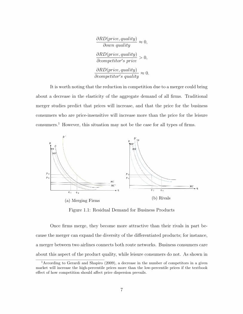
It is worth noting that the reduction in competition due to a merger could bring

about a decrease in the elasticity of the aggregate demand of all firms. Traditional

merger studies predict that prices will increase, and that the price for the business

consumers who are price-insensitive will increase more than the price for the leisure

consumers.1 However, this situation may not be the case for all types of firms.

(a) Merging Firms(b) Rivals

Figure 1.1: Residual Demand for Business Products

Once firms merge, they become more attractive than their rivals in part be-

cause the merger can expand the diversity of the differentiated products; for instance,

a merger between two airlines connects both route networks. Business consumers care

about this aspect of the product quality, while leisure consumers do not. As shown in

1According to Gerardi and Shapiro (2009), a decrease in the number of competitors in a givenmarket will increase the high-percentile prices more than the low-percentile prices if the textbookeffect of how competition should affect price dispersion prevails.

7

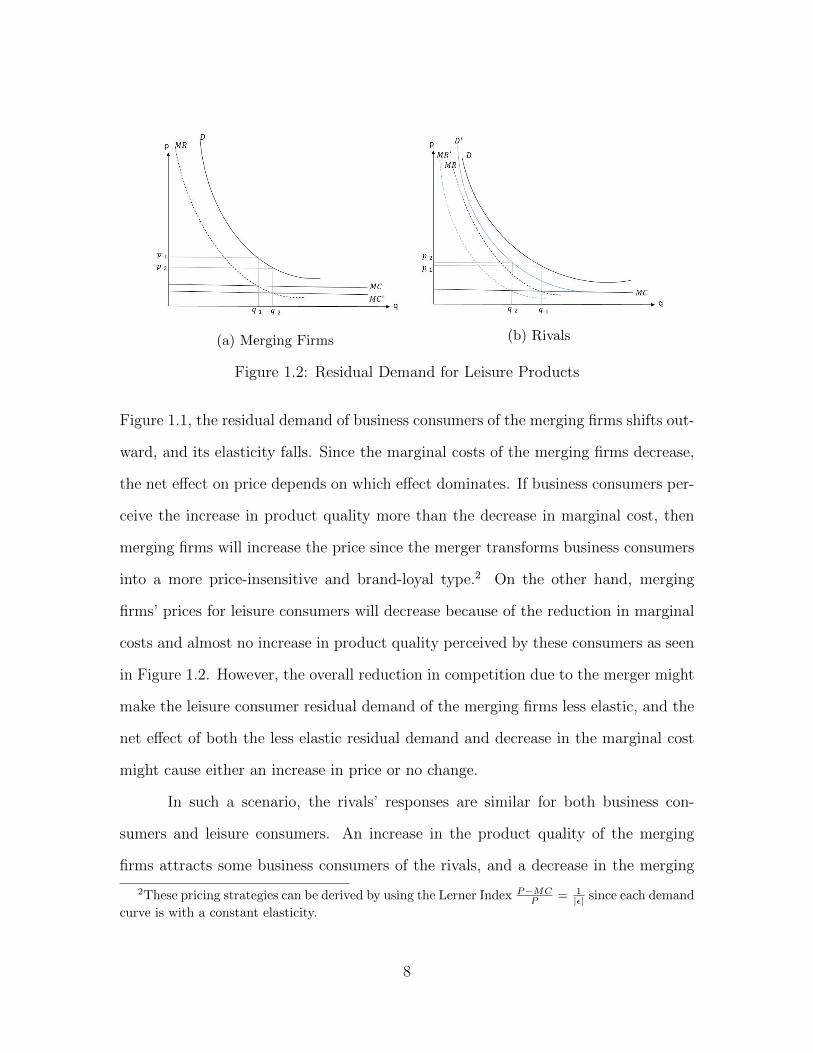
(a) Merging Firms (b) Rivals

Figure 1.2: Residual Demand for Leisure Products

Figure 1.1, the residual demand of business consumers of the merging firms shifts out-

ward, and its elasticity falls. Since the marginal costs of the merging firms decrease,

the net effect on price depends on which effect dominates. If business consumers per-

ceive the increase in product quality more than the decrease in marginal cost, then

merging firms will increase the price since the merger transforms business consumers

into a more price-insensitive and brand-loyal type.2 On the other hand, merging

firms’ prices for leisure consumers will decrease because of the reduction in marginal

costs and almost no increase in product quality perceived by these consumers as seen

in Figure 1.2. However, the overall reduction in competition due to the merger might

make the leisure consumer residual demand of the merging firms less elastic, and the

net effect of both the less elastic residual demand and decrease in the marginal cost

might cause either an increase in price or no change.

In such a scenario, the rivals’ responses are similar for both business con-

sumers and leisure consumers. An increase in the product quality of the merging

firms attracts some business consumers of the rivals, and a decrease in the merging

2These pricing strategies can be derived by using the Lerner Index P−MCP = 1

|ε| since each demand

curve is with a constant elasticity.

8

firms’ price for leisure products attracts price-sensitive leisure consumers from the

rivals. This means that the rivals’ residual demands shifts inward and becomes more

inelastic. Thus, rivals tend to raise prices for both types of consumers, resulting in a

displacement effect caused when merging firms reduce the price for leisure consumers

while competitors increase their prices.

In further empirical analysis, I decompose the market into two types: leisure

markets and big-city markets. Leisure markets primarily consist of leisure consumers,

while big-city markets are composed of both leisure and price-insensitive business con-

sumers. Such markets with different combinations of consumer bases could alter a

firm’s pricing strategies. When merging firms exploit business consumers in big-city

markets by raising their prices, it becomes more difficult to reduce airfares for leisure

consumers. This is because such targeting pricing strategies encourage business con-

sumers to act like leisure consumers and buy tickets at low fares. Rivals can respond

by raising prices for both business consumers and leisure consumers. Specifically,

since there is only one type of consumer in leisure markets, the displacement effect

still holds, with merging firms targeting these consumers with lower prices and rivals

responding by increasing airfares for the remaining brand-loyal leisure consumers.

The intuition is summarized in the following hypotheses:

(a) In leisure markets, merging firms can reduce prices due to the efficiency they

gain from the merger, thus poaching non-brand-loyal customers from their rivals.

Rivals are better off increasing prices because a larger share of their remaining

customers will be brand-loyal consumers.

(b) In big-city markets, merging firms can increase prices for business consumers

when the increase in product quality perceived by those business consumers is

more than the decrease in marginal cost and vice versa. Merging firms will not

9

reduce prices for leisure consumers since group pricing strategies cannot prevent

business consumers from buying tickets as leisure consumers. In this case, rivals

may respond by raising prices only for business consumers.

1.3 Deal Background

In 2008, United Air Lines and Continental Air Lines came close to merging.

However, they negotiated a deal that made Continental a member of the United-

led Star global alliance, filling in the large and lucrative New York City market,

once a weak spot in the Star’s global network.3 Although this agreement was only for

international networks, it was a virtual merger, so defined because it included many of

the benefits of a merger. For instance, United and Continental had antitrust immunity

to operate their international networks jointly. Granted by the U.S. Transportation

Department, the immunity allowed both firms beginning in 2008 to share proprietary

market data, divvy up routes, jointly set prices and negotiate travel contracts with

corporations, and operate on the immunized portions of their networks as if they had

merged.

Because of this initial agreement, when both merging firms suggested the idea

of merging for the second time in 2010, the whole deal went very smoothly. As seen in

Table 1.1, both the Board of Directors at Continental and United Airlines approved a

stock-swap deal that made them the world’s largest airline company on May 2, 2010.

This deal, which was announced the next day, was under investigation for only about

three months before the U.S. Department of Justice approved this $3 billion merger on

one condition, transferring Continental’s slots and other assets at Newark to South-

west. Less than one month later, shareholders of both airlines approved the merger

3USATODAY: Irked US Airways ends merger talks with United.

10

http://usatoday30.usatoday.com/MONEY/usaedition/2010-04-22-us-airways-ends-merger-talks-united-airlines_NU.htm

on September 17, 2010. Approximately two weeks later on October 1, UAL Corpora-

tion, which is the parent company of United Airlines, acquired Continental Airlines,

changing its name to United Continental Holdings, Inc., indicating the completion of

the deal. Both airlines were corporately managed by the same team, although they

remained separated until the operational integration was complete. Approximately

one year later, the Federal Aviation Administration (FAA) issued a single operating

certificate to both merging firms, which allowed them to begin flying as one airline

under the name United. Then both companies started integrating their systems, a

process that was completed on March 3, 2012. The OnePass loyalty program, the

frequent flier program for Continental, was phased out on December 31, 2011.

Both merging parties were influential players in the airline industry. At the

time of the merger, United Airlines, based in Chicago, was the third largest carrier in

the United States in terms of revenue, and Continental Airlines, based in Houston, was

the fourth largest carrier in the United States. In 2009, the year before the merger,

UA earned $16.3 billion in revenue carrying approximately 80 million passengers and

offering service to 230 destinations in the United States and 30 other countries. During

the same year, CO’s income was $12.6 billion, and it carried 67 million passengers,

providing service with its regional affiliates to 265 destinations in the United States

and more than 50 other countries all over the world.

In general, there are two significant categories of carriers: legacy carriers and

low-cost carriers (LCCs); both with very different business models and pricing strate-

gies. Legacy carriers adopt the hub-and-spoke network, while LCCs use the point-to-

point operating practice. Usually, the average fares of LCCs are lower than the legacy

carriers because the former model focuses on business and operational practices to

keep airline costs low, for example by flying a single airplane type (Southwest) and

increasing airplane utilization. Table 1.2 lists these carriers around the sampling pe-

11

riod for the data used in this study. The merging firms UA and CO are both legacy

carriers. In the later analysis, I further decompose carriers into three groups: merg-

ing firms, legacy rivals, and LCC rivals based on Table 1.2. Although there might

be other types of rival carriers providing flight services, such as regional legacy car-

riers like Alaska (AS) and Hawaiian Airlines (HA), these carriers only compete with

both merging firms on a few routes compared to three other national legacy rivals

American (AA), Delta (DL) and US Airways (US) (94 for AS, 2 for HA). 4

1.4 Data

1.4.1 Data Sources

The two primary data sources for this paper are the Airline Origin and Desti-

nation Survey (DB1B) published by the U.S. Department of Transportation and the

T100 Domestic Segment Database (T100). The DB1B database is a 10% quarterly

sample of all domestic tickets issued by U.S. reporting airlines, including information

on origin, destination and connecting airports, marketing carriers, operating carriers,

year, quarter, fare, and number of passengers paying that fare.5 The T100 database,

a supplement to the DB1B from the Bureau of Transportation Statistics, reports ori-

4The estimation results still hold with these airlines included.5I applied several common filters used in the airline economics literature to clean the data and

construct a comparable dataset. Only domestic direct flights are included, which encompasses bothnonstop flights and flights in which there is a stop but no change of airplane. Directionality issuppressed; for example, a flight from Atlanta to Los Angeles is treated the same as a flight fromLos Angeles to Atlanta. A roundtrip itinerary is split into two observations, and the fare is dividedby two. Open-jaw itineraries (where a roundtrip passenger does not return to the origin city)are dropped. Observations with fares of questionable magnitude are dropped, and bulk fares areeliminated as well. Fares greater than five times the DOT’s Standard Industry Fare Level (SIFL)are also excluded. I also dropped all fares that are less than $25 for a one-way trip. Only coach-classtickets are kept. Coupon types indicating foreign carrier flying between 2 U.S. points are dropped.To deal with the issue of code sharing, I dropped flights including a change of ticking carriers andflights in which the operating and ticking carriers are different.

12

gin, destination, carrier, aircraft type and service class for transported passengers,

number of seats, scheduled departures, departures realized by airlines and airport-

pair segments for all domestic passenger flights.6 These data are used to identify the

capacity of direct flights.

My study focuses on domestic, direct, and coach-class airline tickets from 2008:

Q3 to 2011: Q3. Since the UA-CO merger was approved by the Department of Justice

(DOJ) on August 27, 2010 (the third quarter of 2010), this quarter is identified as

t0 in the empirical analysis. However, this t0 is not a subjective cut-point as in

many previous merger studies.7 Eight quarters before t0 and four quarters after t0

are included. The excluded period is between one and two years, that is, the fifth

through eighth quarters, prior to t0. Each of the remaining nine quarters uses a

dummy to capture the dynamic change of price or capacity relative to its average

value in the excluded period. Tables 1.3, 1.4, and 1.5 provide summary statistics

for the price, capacity, and market share variables used in this analysis. These data

suggest that there is no difference in the 10th percentile airfares but a difference in the

90th percentile airfares between the legacy airlines and the LCC airlines in big-city

markets. The average market shares of merging firms are more than twice of both

the legacy and the LCC rivals.

1.4.2 Route Types and Variable Construction

The two primary categories of routes involving United and Continental are

overlapping routes and control routes. The overlapping routes are defined as those be-

ing served by both merging firms, UA and CO, consistently and continuously through-

6As with the DB1B data, the directionality here is suppressed as well. By using the variableaircraft configuration in the dataset, I kept flights of passenger configuration or flights of combinedpassenger and freight on a main deck. Unlike the DB1B, this is a monthly dataset, so I totaledseats, flights and passengers to the year-quarter-route-carrier level.

7Carlton et al. (2016); Kim and Singal (1993).

13

out the sampling period. For the control routes, neither UA nor CO offers flights on

these routes in any quarter of the sampling period. Any non-merging carrier on a

route that is in the included periods, four quarters before and after the approval

quarter as well as the approval quarter, must appear in the excluded period, the fifth

through eighth quarters prior to the approval quarter, as well.

I decompose routes, including overlapping routes and control routes, into two

sub-categories according to the location of airport endpoint(s): leisure routes and

big-city routes. I assume that tickets for routes to tourist destinations are primarily

bought by leisure travelers who are price-sensitive, while tickets for big-city routes

are bought by tourists and business travelers who are price-insensitive. Thus, firms

might adopt different pricing strategies in these two markets due to the difference in

consumer bases.

Using the methods of Gerardi and Shapiro (2009) to distinguish between leisure

routes and big-city routes, I first calculate the ratio of accommodation earnings to

total nonfarm earnings in each metropolitan area (MA) containing airports for the

years 2009 to 2011 and then take the median value from these three ratios.8 Second,

I sort the median ratios, putting them in descending order. An MA is labeled as a

leisure MA when its ratio is above the 90th percentile. Next, a leisure route is defined

as either one of its two airport endpoints located in a leisure MA. Similar to Gerardi

and Shapiro (2009), I include three areas that have no MA earnings data: San Juan,

St. Croix, and St. Thomas. Table 1.6 lists the leisure route sample.

The criterion for selecting the big-city routes is much simpler than the process

for the leisure routes. Based on the data of census 2010, a route is classified as

8These data are obtained from Bureau of Economic Analysis. Table CA5N Personal Income byMajor Component and Earnings by NAICS Industry contains information about industry earningsin all metropolitan statistical areas throughout the United States. These three ratios for three yearscover the entire time span of my data.

14

a big-city one if both its origin and destination airports are located within the 30

largest MAs in terms of population.9 The hub airports of both merging carriers UA

and CO are in these 30 largest MAs. Table 1.7 details the big-city route sample.

Based on these criteria and selection processes, the dataset for this study contains

420 overlapping routes, 112 overlapping leisure routes, 166 overlapping big-city routes,

and 7731 control routes, which include 1422 leisure routes and 69 big-city routes.

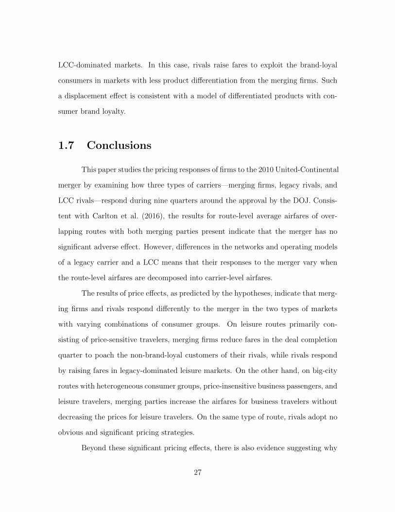
Figure 1.3 and Figure 1.4 show the examples of the price distributions for a

leisure route and a big-city route. These are coach-class nominal airfares during the

third quarter of 2011 on the direct flights of the leisure route from Pittsburgh (PIT) to

Las Vegas (LAS) by Delta and of the big-city route from Pittsburgh (PIT) to Houston

(IAH) by United. The distribution of a leisure route with a single mode and long

right tail indicates the majority of travelers bought tickets around $90, which appears

to be consistent with the assumption that most travelers are leisure consumers. The

histogram of the big-city overlapping route, however, displays a bimodal distribution,

which denotes a large group of travelers bought tickets for approximately $210 and

another large group for roughly $660. This characteristic of the price distribution of

a big-city overlapping route implies both leisure travelers and business travelers are

the targets of the airlines. Additionally, the big-city price distribution shows that

the 10th-20th percentile fare is close to the left mode and the 90th-80th percentile

fare is close to the right mode. Based on these distributions, in the later analysis I

will use the 10th, 15th, and 20th percentile fares to represent prices paid by leisure

passengers and the 80th, 85th, and 90th percentile fares to represent prices paid by

business travelers.10

9Data are from U.S. Census Bureau, Population Division. Miami, Fort Lauderdale, San Diego,Tampa, and Orlando are dropped from the 30 largest MAs list because these areas are primarilysightseeing places. Actually, Miami, Fort Lauderdale and Orlando are in the leisure MAs list.

10Most price distributions of other big-city routes show the same pattern, indicating the choicesof 10th (or 15th, 20th) percentile fare and 90th (or 85th, 80th) percentile fare could be close to the

15

Before the data are collapsed into the carrier-route-year-quarter level, the

DB1B includes multiple fares for the same flight by the same carrier for a specific

quarter of the year. This data structure provides a price distribution for tickets sold

by the same carrier for a flight. From this distribution, I construct seven depen-

dent variables: average airfare, 10th percentile airfare, 15th percentile airfare, 20th

percentile airfare, 80th percentile airfare, 85th percentile airfare, and 90th percentile

airfare. The average airfare is a passenger-weighted price.11 For those percentile

fares, after sorting the fares for the same flight by a specific carrier in each quarter

and putting them in descending order, I obtain the 10th (15th, 20th) percentile airfare

and 90th (80th, 85th) percentile airfare, characterizing the discounted price (or low

price) and the full price (or high price) respectively.12 By merging T100 data with

the DB1B sample,13 I construct the capacity variable, the number of seats available

on a flight by the same carrier in a specific quarter, and the load factor, which is the

share of available seats on the flights with passengers seated in them.

1.5 Model

Different from previous merger case studies that define a subjective timing of

price changes, for instance, the approved quarter by DOJ,14 I use a baseline model

similar to that of Goolsbee and Syverson (2008) and Whinston and Collins (1992).

This model measures the change in pricing strategies for different firms before, during,

and after the merger by letting merger effects differ more finely than by pre- and

left mode and right mode (or medians), respectively.11A fare observation associates with how many passengers bought the ticket at the same price.12Tan (2016) holds similar specifications.13Approximately 23 percent of observations in the DB1B matched. For the reasons for the low

matched rate, please see details in Goolsbee and Syverson (2008) and Gerardi and Shapiro (2009).14Prince and Simon (2017), Carlton et al. (2016), Huschelrath and Muller (2015), Luo (2014),

Kwoka and Shumilkina (2010), Kim and Singal (1993).

16

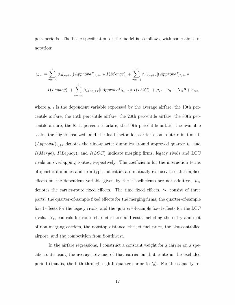
post-periods. The basic specification of the model is as follows, with some abuse of

notation:

ycrt =4∑

τ=−4

βM,t0+τ [(Approval)t0+τ ∗ I(Merge)] +4∑

τ=−4

βLY,t0+τ [(Approval)t0+τ∗

I(Legacy)] +4∑

τ=−4

βLC,t0+τ [(Approval)t0+τ ∗ I(LCC)] + µcr + γt +Xrtθ + εcrt,

where ycrt is the dependent variable expressed by the average airfare, the 10th per-

centile airfare, the 15th percentile airfare, the 20th percentile airfare, the 80th per-

centile airfare, the 85th percentile airfare, the 90th percentile airfare, the available

seats, the flights realized, and the load factor for carrier c on route r in time t.

(Approval)t0+τ denotes the nine-quarter dummies around approved quarter t0, and

I(Merge), I(Legacy), and I(LCC) indicate merging firms, legacy rivals and LCC

rivals on overlapping routes, respectively. The coefficients for the interaction terms

of quarter dummies and firm type indicators are mutually exclusive, so the implied

effects on the dependent variable given by these coefficients are not additive. µcr

denotes the carrier-route fixed effects. The time fixed effects, γt, consist of three

parts: the quarter-of-sample fixed effects for the merging firms, the quarter-of-sample

fixed effects for the legacy rivals, and the quarter-of-sample fixed effects for the LCC

rivals. Xrt controls for route characteristics and costs including the entry and exit

of non-merging carriers, the nonstop distance, the jet fuel price, the slot-controlled

airport, and the competition from Southwest.

In the airfare regressions, I construct a constant weight for a carrier on a spe-

cific route using the average revenue of that carrier on that route in the excluded

period (that is, the fifth through eighth quarters prior to t0). For the capacity re-

17

gressions, a similar method is used to construct the traffic weight for a carrier on a

route. The reason for using both weights is that from a carriers perspective, much

more attention is paid to those routes that can generate high revenue or have heavy

traffic. I also cluster the standard errors at the carrier-route level to account for het-

eroscedasticity and for correlation across observations for a particular carrier-route

combination over time.

The control group for airfare regressions of leisure routes is the leisure control

group, and the control group for airfare regressions of big-city routes is the big-city

control group. Unlike the airfare regressions, for capacity regressions of either leisure

routes or big-city routes, the control group is routes with at least two legacy carriers

and at least one LCC present. The reason for not using the same control group as

for airfare regressions is that these three types of carriers display utterly different

capacity trends in both the excluded period, the fifth through eighth quarters prior

to approval quarter, and the whole sampling period.

The nine covariates of interest for determining the responses of the merging

firms, legacy rivals, and LCC rivals in the merger event are βM,t0+τ , βLY,t0+τ , and

βLC,t0+τ . These coefficients include four quarters before approval, four quarters after

approval, and the approval quarter. It is appropriate to use such an event window

since the UA-CO merger is announced in t0 − 1, approved in t0 and completed in

t0 + 1. Firms anticipate a high chance of deal approval by DOJ based on the con-

nection between UA-CO in the virtual merger agreement in 2008. In addition, these

coefficients explain whether merging firms, legacy rivals, or LCC rivals respond to

the merger differently from their average values in the excluded period relative to the

control group.

As discussed previously, the conventional view of a merger’s price impact fo-

cuses on the average market prices or the average prices of merging firms and their

18

rivals, without considering the types of markets or different consumer groups.15 This

empirical analysis assesses the firms’ pricing strategies in leisure markets with pri-

marily leisure travelers and big-city markets with both business and leisure travelers.

To test the Hypotheses (a) and (b), I treat tickets in leisure markets as primarily

bought by leisure travelers. In big-city markets, the 80th, 85th, and 90th percentile

airfares of a carrier on a route represent prices charged for business travelers, and

the 10th, 15th, and 20th percentile airfares represent prices paid by leisure travelers.

In addition to the price regressions, I also analyze the capacity strategies of firms in

both types of markets to determine if they are adjusting capacity to maintain their

pricing strategies.

1.6 Empirical Results

1.6.1 Price Regressions

Tables 1.8 through 1.13 present the results from estimating the baseline model

in different markets and with different dependent variables, with each table repre-

senting a single estimation. To compare the coefficients conveniently, I put those for

merging firms, legacy rivals, and LCC rivals into three columns. To visualize the

firms’ responses to the merger, I also created price paths based on the coefficients

for the interaction terms of quarter dummies and firm type indicators (Figures 1.5

through 1.9).

Table 1.8 is a partial replication of Carlton et al. (2016) with a 9-quarter event

window and the fifth through eighth quarters prior to t0 as an excluded period. The

results show the average market fare only trending up and down. It seems that there

15Borenstein (1990), Kim and Singal (1993), and Carlton et al. (2016) only consider the overlappingroutes where both merging parties are present.

19

is a rise at t0, but the coefficient is not significantly different from the coefficients

for t0-1, t0-2, t0-3, and t0-4 at the 5% level. This result is consistent with Carlton

et al. (2016), who conclude that the UA-CO merger has no significant price effect

on overlapping routes. However, after the market-level price is decomposed into the

firm-level price, the results seen in Table 1.9 indicate an entirely different scenario.

Both merging firms and legacy rivals significantly increase fares in anticipation of the

merger’s approval,16 with the fares remaining at these high levels. However, the LCC

rivals do not change their fares significantly. These results imply that the analysis

conducted by Carlton et al. (2016) may be incomplete. By the time the merger is

approved by DOJ, the fares of merging firms on overlapping routes are 14.8% 17 above

the excluded period relative to the control routes, and the legacy rivals are 12.1%

higher. On average, the percentage change in price is above 8% for both merging

firms and legacy rivals. Although the legacy rivals might not display a significant

increasing pattern here, a clear pattern is found in the leisure markets.

The results of leisure routes are consistent with Hypothesis (a) (see Table 1.10).

Merging firms begin reducing fares after the approval, even though the coefficients of

t0+2 and t0+3 are not significant. It is noted that t0+1 represents the quarter the deal

is completed, suggesting that merging firms see efficiency gains after the completion

period when both UA and CO are corporately controlled by the same leadership.

Kim and Singal (1993) find similar results in their studies of 14 mergers from the

1980s. Conversely, the legacy rivals respond by beginning to increase fares in the deal

16Borenstein (1990), Kim and Singal (1993), and Prager and Hannan (1998) found the timing ofprice increases is before the merging firms allowed to coordinate their operation legally. Weinberg(2007) explains this phenomenon using the standard models of switching costs, in which firms initiallyprice low to gain market share and later extract consumer surplus by increasing prices. This switchingcost plays a role in locking consumers initially. When two firms merge, there is uncertainty concerningthe future of management teams in the newly merged firm, so the incentive to invest in the marketshare is lost because managers may lose their jobs as a result of restructuring and not realize areturn from this investment.

17exp(0.138)-1

20

announcement period t0-1, and, on average, the fares are approximately 10% higher

than in the excluded period relative to the control group. The LCC rivals show no

significant evidence of rising or declining fares. These patterns seem to imply that

product substitution between two legacy carriers is greater than that between a legacy

carrier and a low-cost carrier. This suggests that perhaps the low-price strategy of

merging firms primarily focuses on poaching price-sensitive passengers from legacy

rivals in leisure markets. By raising fares, the legacy rivals seem to respond by

exploiting their brand-preferred leisure travelers, such as those consumers enrolled

in frequent-flyer programs, to maximize profits. Empirical results from the leisure

markets support the existence of the displacement effect even when the number of

firms decreases.

The two major groups of travelers in big-city markets, business travelers and

leisure travelers, are pooled in Table 1.11, which presents results from estimating the

average logged fares. Results indicate that merging firms begin raising fares one quar-

ter before the announcement period t0-1, legacy rivals’ responses are negligible since

most coefficients are indifferent from zero at the 5% level, and the coefficients in the

LCC rivals column are constant at approximately -44%. To look closely at the firms’

pricing strategies for both leisure and business travelers on big-city routes, the 10th,

15th, and 20th percentile airfares are used to represent the prices charged for low-fare

leisure travelers, and the 80th, 85th, and 90th percentile airfares represent the prices

paid by high-fare business travelers, as suggested in the previous data section. The

regression results for leisure travelers using 10th, 15th, and 20th percentile airfares

are very similar, and regression results for business passengers using 80th, 85th, and

90th percentile airfares are identical as well. Thus, only the results of 15th and 85th

percentile airfares are presented in Tables 1.12 and 1.13, respectively.

As seen in Tables 1.12, merging firms increase their fares for leisure travelers in

21

big-city markets only in the announcement quarter and the approval quarter, then the

effects return to zero quickly, which implies that merging firms do not apply a stable

pricing rule to target leisure travelers. Similarly, neither legacy rivals nor LCC rivals

have significant pricing patterns. Coefficients for legacy rivals trend up and down.

However, in Table 1.13, merging firms begin increasing fares for business travelers

in quarter t0-2, with their coefficients remaining steady in the higher percentages.

Although legacy rivals seem to reduce prices for business travelers a little around

10%, most of the coefficients are neither significant nor significantly different from

zero. The coefficients for LCC rivals move up and down around -0.55, indicating no

significant pricing pattern. The empirical results for merging firms in big-city mar-

kets are consistent with Hypothesis (b), that is, merging firms raise fares for business

travelers without adjusting fares for leisure travelers and both types of rivals show no

significant changes in airfares for business travelers and leisure travelers. One reason

for their lack of significant response could be that there are no network advanta-

geous gains for them through the merger, and their network might even become less

favourable compared to merging firms.

In conclusion, due to the efficiency gains from the merger, merging firms adopt

a low-price strategy in leisure markets to attract price-sensitive passengers, and legacy

rivals respond by raising fares. In big-city markets, merging firms increase prices only

for the business travelers but do not reduce airfares for the leisure passengers. This

strategy avoids business travelers pretending to be leisure travelers and buying tickets

at lower prices. However, both types of rivals exhibit no significant responses in their

pricing strategies.

22

1.6.2 Capacity Regressions

Tables 1.14 through 1.19 show the results of capacity regressions using the

T100 data. These regressions test whether firms adopt specific capacity strategies

to maintain or support their pricing strategies in response to the merger. The re-

gressions use three dependent variables of available seats, flights realized, and load

factor for both types of overlapping markets, leisure markets and big-city markets.

This T100 dataset, as a supplement to the analysis of the firms’ pricing strategies, is

composed of the number of passengers, flights, and available seats by segment-carrier-

month, which are initially aggregated by route-carrier-quarter and then matched with

the DB1B observations. It is important to note that some of the coefficients are not

conventionally significant, specifically for the results of available seats and flights real-

ized.18 This lack of statistical significance is probably a consequence of the weaknesses

in the low match rate between the DB1B data and the T100 data.

Both Table 1.14 and Table 1.15 show similar patterns for merging firms and

legacy rivals. Throughout the entire nine quarters around the approval period, it

is probable that merging firms expand capacities regarding both available seats and

flights for leisure routes, given the point estimates and the precision of the coefficients.

On the other hand, legacy rivals begin reducing capacity from the announcement

quarter t0-1. However, unlike for merging firms or legacy rivals, there is no evidence

to support a clear and steady capacity strategy for LCC rivals. Table 1.16 presents

the dynamic changes in the load factor (defined as the share of available seats on

the flights with passengers in them). Although merging firms expand capacity, the

load factor increases significantly. This trend implies that the increase in passengers

attracted to merging firms due to a low-fare strategy is more than the increase in

18The capacity estimations with respect to available seats and flights in Goolsbee and Syverson(2008) have a similar issue about the coefficients.

23

capacity. For the legacy rivals, the load factor appears to begin to fall after cutting

capacity, perhaps indicating a decrease in passengers due to an increase in fares

for leisure travelers more than the decrease in capacity. As has been demonstrated

previously in the price regressions section, merging firms decrease fares while legacy

rivals increase prices in leisure markets. The results for capacity show that firms

adopt capacity strategies to maintain their pricing strategies on leisure routes.

The results for capacity change in big-city markets are shown in Tables 1.17

through 1.19. Unlike in the leisure markets, merging firms adopt a different capacity

strategy here. Their capacity on big-city routes tends to shrink, which is consistent

with their pricing strategy of increasing fares for business travelers without adjusting

fares for leisure passengers. Capacities for both legacy rivals and LCC rivals provide

no clues concerning capacity changes, only showing an up and down trend since they

have no steady and significant pricing responses on big-city routes. As seen in Table

1.19, the load factors for all three types of firms do not show a clear trend. This

situation is probably caused by a lack of distinction in the data between the capacity

for business travelers and leisure travelers in big-city markets.

1.6.3 Testing Potential Causes for Price Changes in Leisure

Markets

In a traditional merger analysis, the prices usually go up due to the reduction

in competition. However, the results of the estimations for leisure markets show

that merging firms appear to poach customers from legacy rivals by reducing fares

and expanding capacity, with legacy rivals responding by significantly increasing fares.

Different responses among merging firms, legacy rivals, and LCC rivals seem to reflect

the various potential causes of price changes.

24

Airline companies are differentiated along many dimensions, including brand,

airport share, ticket price, service quality, network, and frequent-flyer program, among

others. In such a differentiated product market, prices can go up or down, depending

on consumer preferences and substitution patterns. Here the preferences are char-

acterized by heterogeneous consumer segments: brand-loyal passengers enrolled in

frequent-flyer programs and passengers concerned only with prices. Under price com-

petition, every firm’s optimal price increases in the share of its brand-loyal consumers

and its competitor’s share of brand-loyal consumers, and decreases in the share of

non-brand-loyal consumers (Klemperer, 1987a; Hastings, 2004).

It is possible that the share of brand-loyal customers is higher in a legacy-

dominated market than in an LCC-dominated market due to the intense price com-

petition from LCCs. By using the market share of LCC rivals as a criterion to de-

compose the leisure routes into two categories; routes with the market share of LCC

rivals higher than 50% and those under 50%,19 I am able to distinguish brand-loyal

consumers from non-brand-loyal consumers. Table 1.20 shows the summary statistics

for both categories of leisure routes. The average airfares of merging firms, legacy

rivals, and LCC rivals on LCC-dominated routes and the average airfare of LCC ri-

vals on legacy-dominated routes are very close, even with their standard deviations

being at the same level. However, average fares of both merging firms and legacy

rivals on legacy-dominated routes are much higher than those four similar average

airfares. These statistics indicate there may be one type of price-sensitive consumer

in a market with a high share of LCCs, and two types of consumers in a market with

a low percentage of LCCs, specifically brand-loyal passengers and price-sensitive pas-

sengers. According to the above theory, when two legacy carriers merge, equilibrium

19This threshold is not critical as the summary statistics (Table 1.20) and later price regressions(Tables 1.21 and 1.22) are not sensitive to it. I also tried routes with LCC rivals market sharegreater than 60% (70%) or less than 40% (30%) and did not find significantly different results.

25

prices will increase more in a market with a low share of LCCs than in a market with

a high share of LCCs, under the assumption that most consumers of an LCC are

price-sensitive passengers.

Tables 1.21 and 1.22 present results for these two categories of leisure routes

based on an estimation of the baseline model using the logged average fares. Com-

paring these two tables indicates that both legacy rivals and LCC rivals raise prices

significantly in legacy-dominated markets, but not in LCC-dominated markets. Ad-

ditionally, the results for merging firms on legacy-dominated routes are similar to the

results in Table 1.10 that pool the markets together with both high and low share

of LCCs, that is, merging firms begin reducing fares in t0+1 to attract the price-

sensitive passengers. In light of the merging firms’ potential incentive to expand their

market, legacy rivals raise fares to approximately 11% higher than in the excluded

period relative to the control group. In contrast to their insignificant coefficients seen

in Table 1.10, LCC rivals increase their fares significantly for approximately three

quarters. Here, the substantial effect of reduction in competition due to the merger

in legacy-dominated markets and loyal passengers enrolled in frequent flyer programs

of LCCs could contribute to the significant response of the LCC rivals. In contrast,

on the LCC-dominated routes, none of the coefficients of these three types of carriers

is different from zero at a 5% level. Merging firms seem to raise fares, and both legacy

rivals and LCC rivals show no clear responses.

The patterns of merging firms lend some evidence to support that they tend

to poach non-brand-loyal customers of both legacy rivals and LCC rivals in markets

with high shares of legacy carriers. This pricing strategy of merging firms could be

an attempt to target the customers of legacy rivals since no clear and significant

pattern is displayed in LCC-dominated markets. Another reason is that the prod-

uct differentiation in legacy-dominated markets is smaller for merging firms than in

26

LCC-dominated markets. In this case, rivals raise fares to exploit the brand-loyal

consumers in markets with less product differentiation from the merging firms. Such

a displacement effect is consistent with a model of differentiated products with con-

sumer brand loyalty.

1.7 Conclusions

This paper studies the pricing responses of firms to the 2010 United-Continental

merger by examining how three types of carriers—merging firms, legacy rivals, and

LCC rivals—respond during nine quarters around the approval by the DOJ. Consis-

tent with Carlton et al. (2016), the results for route-level average airfares of over-

lapping routes with both merging parties present indicate that the merger has no

significant adverse effect. However, differences in the networks and operating models

of a legacy carrier and a LCC means that their responses to the merger vary when

the route-level airfares are decomposed into carrier-level airfares.

The results of price effects, as predicted by the hypotheses, indicate that merg-

ing firms and rivals respond differently to the merger in the two types of markets

with varying combinations of consumer groups. On leisure routes primarily con-

sisting of price-sensitive travelers, merging firms reduce fares in the deal completion

quarter to poach the non-brand-loyal customers of their rivals, while rivals respond

by raising fares in legacy-dominated leisure markets. On the other hand, on big-city

routes with heterogeneous consumer groups, price-insensitive business passengers, and

leisure travelers, merging parties increase the airfares for business travelers without

decreasing the prices for leisure travelers. On the same type of route, rivals adopt no

obvious and significant pricing strategies.

Beyond these significant pricing effects, there is also evidence suggesting why

27

firms maintain such pricing strategies. Specifically, merging firms appear to expand

capacity on leisure routes and reduce their capacity on big-city routes to maintain

their respective pricing strategies. The capacity for legacy rivals in leisure markets

tends to shrink to support their high-fare strategy, while their capacity in big-city

markets displays no steady trend. The analysis of the load factor reveals more about

the incentives behind the firms’ pricing strategies. The significant increasing trend

of the load factor on leisure routes implies that merging parties gain market shares

based on the low-fare rule. However, the load factor for legacy rivals seems to begin to

fall after they reduce their capacity in leisure markets. This could mean that legacy

rivals abandon a fraction of price-sensitive non-brand-loyal leisure travelers and earn

more revenue with lower costs by exploiting their remaining brand-loyal customers.

In big-city markets, there is no clear and distinct trend for firms regarding the load

factor, likely, because of the lack of distinction between the capacity for business and

leisure passengers. Perhaps, merging firms want to improve their financial situations

by generating a stable cash-flow from business travelers on big-city routes to address

their losses from the recession in 2008 and 2009.

This paper’s findings suggest that the displacement effect can be present in

a situation involving a reduction in competition. In leisure markets when merging

firms reduce airfares, legacy rivals increase prices. Such responses are consistent

with a model of differentiated products with consumer brand loyalty. In addition,

Kim and Singal (1993) hypothesize that for all types of overlapping markets, the

market-power effect dominates during the announcement period, whereas the joint

and offsetting effects of market power and efficiency gains come into play during

the merger deal completion period. In contrast, the results in this paper show that

merging firms can take advantage of both effects simultaneously in different markets

by targeting a particular consumer group with different pricing strategies. Future

28

research on mergers in other oligopolistic industries may help to reveal how often

mergers generate significant displacement effects.

29

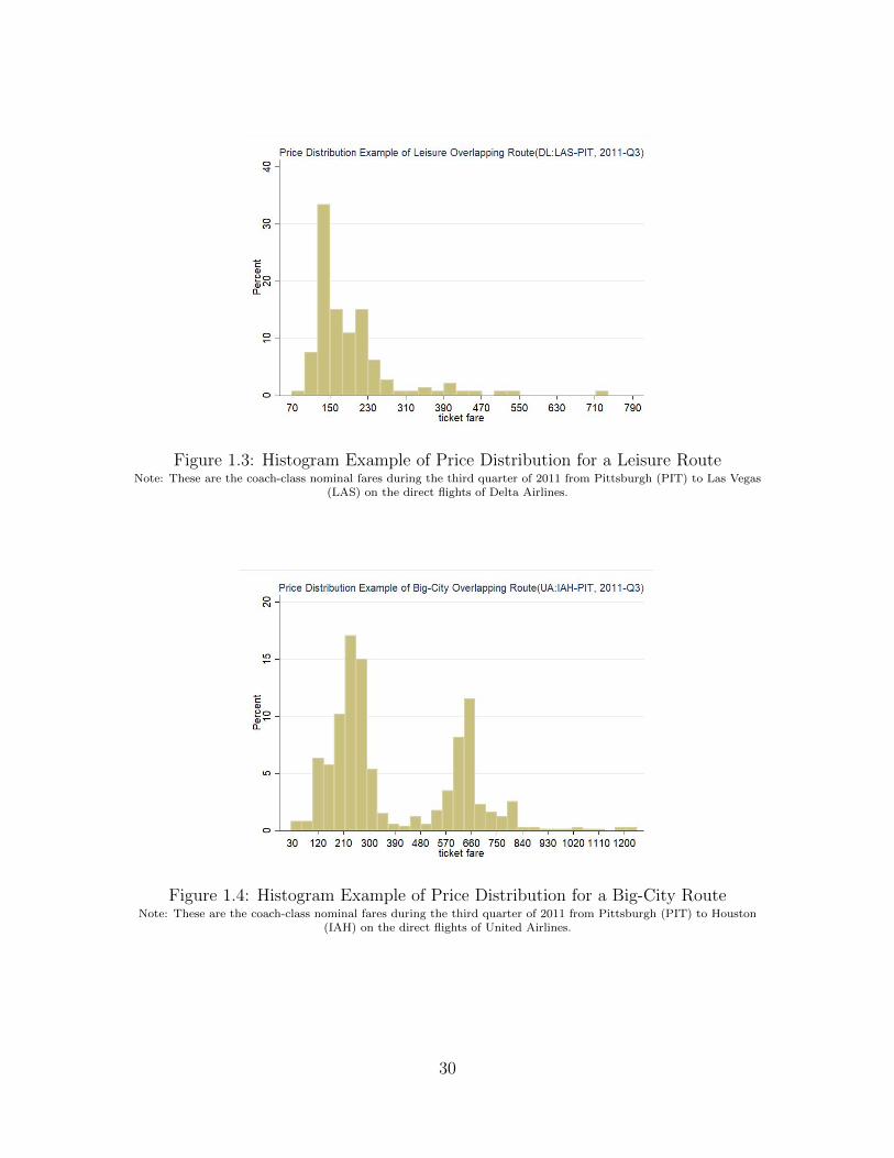
Figure 1.3: Histogram Example of Price Distribution for a Leisure RouteNote: These are the coach-class nominal fares during the third quarter of 2011 from Pittsburgh (PIT) to Las Vegas

(LAS) on the direct flights of Delta Airlines.

Figure 1.4: Histogram Example of Price Distribution for a Big-City RouteNote: These are the coach-class nominal fares during the third quarter of 2011 from Pittsburgh (PIT) to Houston

(IAH) on the direct flights of United Airlines.

30

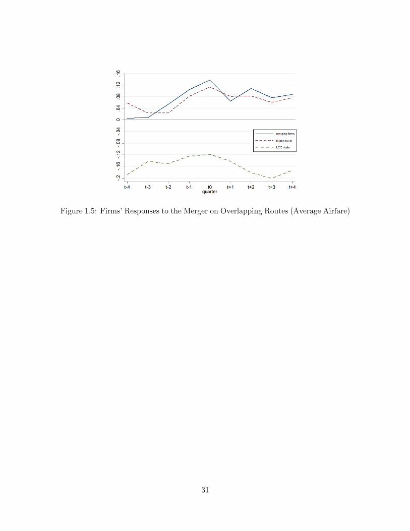
Figure 1.5: Firms’ Responses to the Merger on Overlapping Routes (Average Airfare)

31

Figure 1.6: Firms’ Responses to the Merger on Leisure Routes (Average Airfare)

Figure 1.7: Firms’ Responses to the Merger on Big-City Routes (Average Airfare)

32

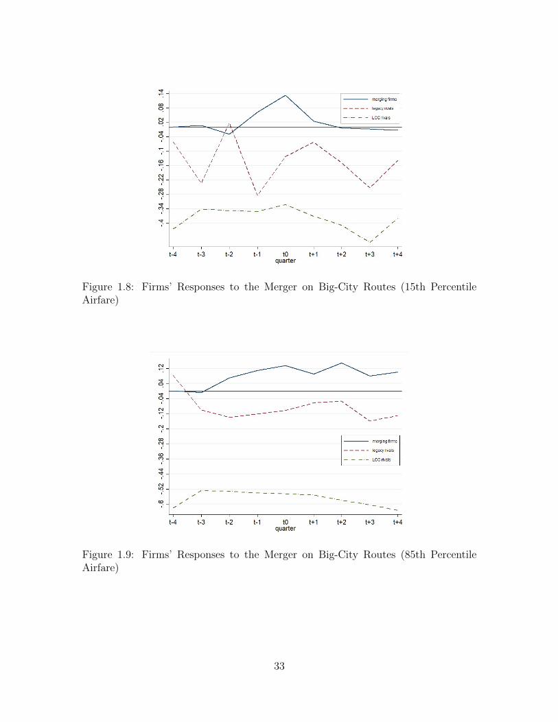
Figure 1.8: Firms’ Responses to the Merger on Big-City Routes (15th PercentileAirfare)

Figure 1.9: Firms’ Responses to the Merger on Big-City Routes (85th PercentileAirfare)

33

Table 1.1: Stages of the Merger Deal

Early 2008 “Virtual Merger”May 3, 2010 AnnouncementAug. 27, 2010 Approval of DOJOct. 1, 2010 Deal CompletedNov. 30, 2011 Operating Certificate of FAAMarch 3, 2012 System Integration & CO OnePass Phased Out

Table 1.2: Carriers and their Categories

Type Code Carrier

Legacy(5)

AA American AirlinesCO Continental Air Lines (M)DL Delta Air LinesUA United Air Lines (M)US US Airways

LCC(9)

B6 JetBlue AirwaysF9 Frontier AirlinesFL AirTran AirwaysG4 Allegiant AirNK Spirit Air LinesSY Sun Country AirlinesTZ ATA AirlinesVX Virgin AmericaWN Southwest Airlines

Note: Carriers with M in the parentheses are marked as mergingfirms.

34

Table 1.3: Summary Statistics (Route-Level)

Variable Route TypeOverlap Leisure Big-City Control

Average Airfare 222.804 231.992 226.313 232.020(75.667) (99.343) (70.052) (132.467)

Available Seats 65437.63 57744.43 84121.16 83670.25(82829.22) (68290.07) (95043.71) (102581.1)

Load Factor 0.8144 0.84037 0.8008 0.7922(0.1736) (0.1403) (0.174) (0.1302)

Note: Standard deviations are in parentheses.

Table 1.4: Summary Statistics (Leisure Routes)

Variable Leisure RoutesMerging Firms Legacy Rivals LCC Rivals

Average Airfare 239.261 247.121 183.186(95.275) (103.134) (47.261)

Available Seats 70881.6 61769.81 43627.92(79812) (79105.3) (28991.8)

Load Factor 0.8513 0.8356 0.8404(0.121) (0.146) (0.141)

Market Share 0.251 0.172 0.171(0.262) (0.225) (0.259)


35

Table 1.5: Summary Statistics (Big-City Routes)

Variable Big-City RoutesMerging Firms Legacy Rivals LCC Rivals

Average Airfare 235.120 234.622 191.87(55.742) (67.057) (49.568)

10th Percentile Airfare 137.547 144.426 133.805(29.960) (54.616) (44.413)

90th Percentile Airfare 425.996 384.427 291.190(155.949) (145.71) (83.64)

Available Seats 98543.66 86701.99 51830.77(95355.48) (104492.7) (39254.61)

Load Factor 0.827 0.790 0.788(0.120) (0.188) (0.205)

Market Share 0.351 0.156 0.123(0.327) (0.234) (0.178)


36

Table 1.6: Leisure Routes Sample

MA Airport Accommodation/Nonfarm Earnings (median)Atlantic City-Hammonton, NJ ACY 0.2042612Las Vegas-Henderson-Paradise, NV LAS 0.1566679Kahului-Wailuku-Lahaina, HI OGG 0.1479694Reno, NV RNO 0.0460088Myrtle Beach-Conway-North Myrtle Beach, SC-NC MYR 0.0456113Flagstaff, AZ FLG 0.0386447Gulfport-Biloxi-Pascagoula, MS GPT 0.0386114Brunswick, GA BQK 0.0365357Lake Charles, LA LCH 0.0297182Orlando-Kissimmee-Sanford, FL MCO 0.0295822Napa, CA APC 0.0279597Salinas, CA MRY 0.0251734Urban Honolulu, HI HNL 0.0238568Santa Fe, NM SAF 0.0233381Hilton Head Island-Bluffton-Beaufort, SC SAV 0.0216004St. George, UT SGU 0.0187629Memphis, TN-MS-AR MEM 0.0166779Bend-Redmond, OR RDM 0.0166375Panama City, FL PFN 0.0153526San Luis Obispo-Paso Robles-Arroyo Grande, CA SBP 0.0152183New Orleans-Metairie, LA MSY 0.0137413Miami-Fort Lauderdale-West Palm Beach, FL MIA FLL PBI 0.013192Wenatchee, WA EAT 0.0128621Rapid City, SD RAP 0.0127379Asheville, NC AVL 0.0127143Santa Maria-Santa Barbara, CA SBA 0.0126143(90th percentile)San Juan, PR SJU N/ASt. Croix, VI STX N/ASt. Thomas, VI STT N/A

37

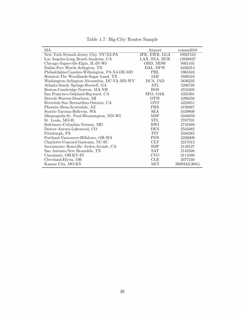
Table 1.7: Big-City Routes Sample

MA Airport census2010New York-Newark-Jersey City, NY-NJ-PA JFK, EWR, LGA 19567410Los Angeles-Long Beach-Anaheim, CA LAX, SNA, BUR 12828837Chicago-Naperville-Elgin, IL-IN-WI ORD, MDW 9461105Dallas-Fort Worth-Arlington, TX DAL, DFW 6426214Philadelphia-Camden-Wilmington, PA-NJ-DE-MD PHL 5965343Houston-The Woodlands-Sugar Land, TX IAH 5920416Washington-Arlington-Alexandria, DC-VA-MD-WV DCA, IAD 5636232Atlanta-Sandy Springs-Roswell, GA ATL 5286728Boston-Cambridge-Newton, MA-NH BOS 4552402San Francisco-Oakland-Hayward, CA SFO, OAK 4335391Detroit-Warren-Dearborn, MI DTW 4296250Riverside-San Bernardino-Ontario, CA ONT 4224851Phoenix-Mesa-Scottsdale, AZ PHX 4192887Seattle-Tacoma-Bellevue, WA SEA 3439809Minneapolis-St. Paul-Bloomington, MN-WI MSP 3348859St. Louis, MO-IL STL 2787701Baltimore-Columbia-Towson, MD BWI 2710489Denver-Aurora-Lakewood, CO DEN 2543482Pittsburgh, PA PIT 2356285Portland-Vancouver-Hillsboro, OR-WA PDX 2226009Charlotte-Concord-Gastonia, NC-SC CLT 2217012Sacramento–Roseville–Arden-Arcade, CA SMF 2149127San Antonio-New Braunfels, TX SAT 2142508Cincinnati, OH-KY-IN CVG 2114580Cleveland-Elyria, OH CLE 2077240Kansas City, MO-KS MCI 2009342(30th)

38

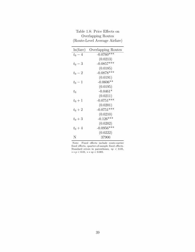
Table 1.8: Price Effects onOverlapping Routes

(Route-Level Average Airfare)

ln(fare) Overlapping Routest0 − 4 -0.0760***

(0.0213)t0 − 3 -0.0857***

(0.0185)t0 − 2 -0.0878***

(0.0191)t0 − 1 -0.0606**

(0.0195)t0 -0.0461*

(0.0211)t0 + 1 -0.0751***

(0.0201)t0 + 2 -0.0751***

(0.0210)t0 + 3 -0.126***

(0.0202)t0 + 4 -0.0956***

(0.0222)N 37900

Note: Fixed effects include route-carrierfixed effects, quarter-of-sample fixed effects.Standard errors in parentheses, ∗p < 0.05,∗ ∗ p < 0.01, ∗ ∗ ∗p < 0.001.

39

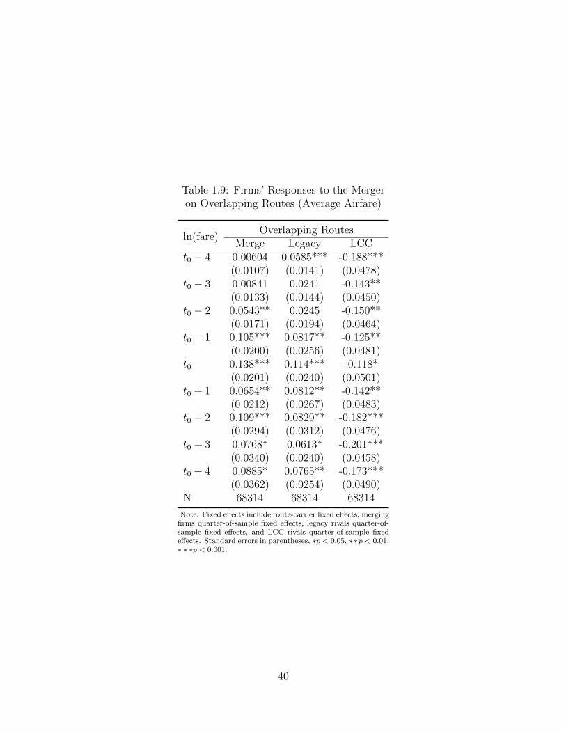
Table 1.9: Firms’ Responses to the Mergeron Overlapping Routes (Average Airfare)

ln(fare)Overlapping Routes

Merge Legacy LCCt0 − 4 0.00604 0.0585*** -0.188***

(0.0107) (0.0141) (0.0478)t0 − 3 0.00841 0.0241 -0.143**

(0.0133) (0.0144) (0.0450)t0 − 2 0.0543** 0.0245 -0.150**

(0.0171) (0.0194) (0.0464)t0 − 1 0.105*** 0.0817** -0.125**

(0.0200) (0.0256) (0.0481)t0 0.138*** 0.114*** -0.118*

(0.0201) (0.0240) (0.0501)t0 + 1 0.0654** 0.0812** -0.142**

(0.0212) (0.0267) (0.0483)t0 + 2 0.109*** 0.0829** -0.182***

(0.0294) (0.0312) (0.0476)t0 + 3 0.0768* 0.0613* -0.201***

(0.0340) (0.0240) (0.0458)t0 + 4 0.0885* 0.0765** -0.173***

(0.0362) (0.0254) (0.0490)N 68314 68314 68314

Note: Fixed effects include route-carrier fixed effects, mergingfirms quarter-of-sample fixed effects, legacy rivals quarter-of-sample fixed effects, and LCC rivals quarter-of-sample fixedeffects. Standard errors in parentheses, ∗p < 0.05, ∗∗p < 0.01,∗ ∗ ∗p < 0.001.

40

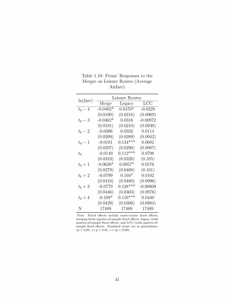
Table 1.10: Firms’ Responses to theMerger on Leisure Routes (Average

Airfare)

ln(fare)Leisure Routes

Merge Legacy LCCt0 − 4 -0.0462* 0.0470* -0.0229

(0.0190) (0.0216) (0.0969)t0 − 3 -0.0462* 0.0316 -0.00972

(0.0181) (0.0210) (0.0930)t0 − 2 -0.0396 0.0332 0.0114

(0.0209) (0.0289) (0.0942)t0 − 1 -0.0181 0.134*** 0.0682

(0.0297) (0.0296) (0.0987)t0 -0.0149 0.112*** 0.0798

(0.0319) (0.0326) (0.105)t0 + 1 -0.0620* 0.0957* 0.0576

(0.0279) (0.0408) (0.101)t0 + 2 -0.0799 0.104* 0.0102

(0.0410) (0.0480) (0.0996)t0 + 3 -0.0779 0.128*** -0.00809

(0.0446) (0.0303) (0.0876)t0 + 4 -0.109* 0.116*** 0.0440

(0.0429) (0.0300) (0.0984)N 17489 17489 17489

Note: Fixed effects include route-carrier fixed effects,merging firms quarter-of-sample fixed effects, legacy rivalsquarter-of-sample fixed effects, and LCC rivals quarter-of-sample fixed effects. Standard errors are in parentheses,∗p < 0.05, ∗ ∗ p < 0.01, ∗ ∗ ∗p < 0.001.

41

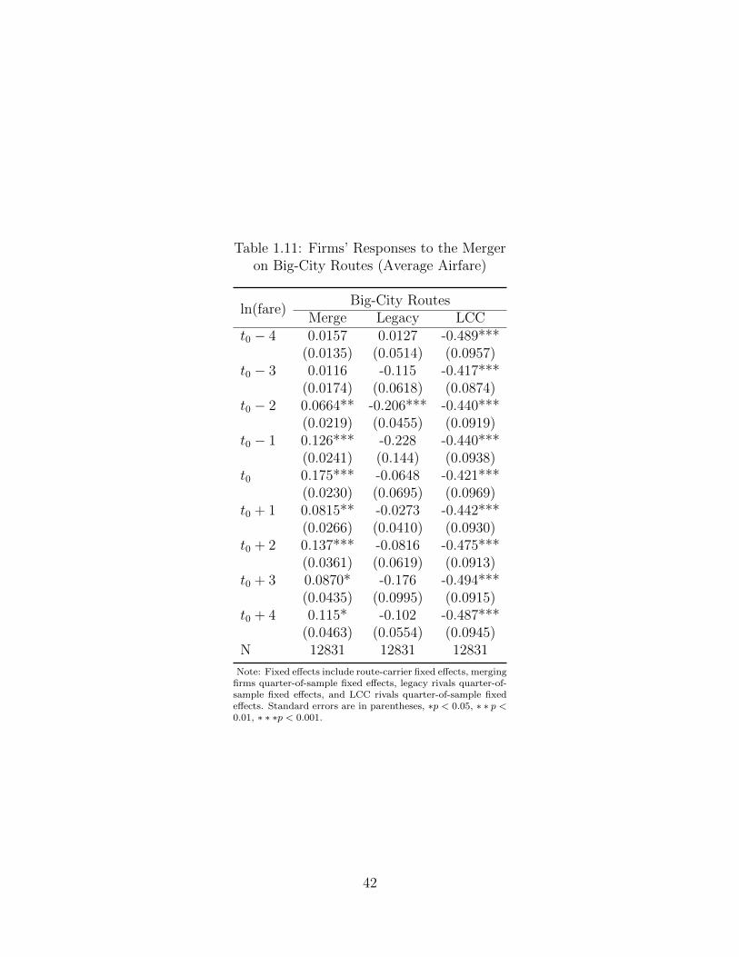
Table 1.11: Firms’ Responses to the Mergeron Big-City Routes (Average Airfare)

ln(fare)Big-City Routes

Merge Legacy LCCt0 − 4 0.0157 0.0127 -0.489***

(0.0135) (0.0514) (0.0957)t0 − 3 0.0116 -0.115 -0.417***

(0.0174) (0.0618) (0.0874)t0 − 2 0.0664** -0.206*** -0.440***

(0.0219) (0.0455) (0.0919)t0 − 1 0.126*** -0.228 -0.440***

(0.0241) (0.144) (0.0938)t0 0.175*** -0.0648 -0.421***

(0.0230) (0.0695) (0.0969)t0 + 1 0.0815** -0.0273 -0.442***

(0.0266) (0.0410) (0.0930)t0 + 2 0.137*** -0.0816 -0.475***

(0.0361) (0.0619) (0.0913)t0 + 3 0.0870* -0.176 -0.494***

(0.0435) (0.0995) (0.0915)t0 + 4 0.115* -0.102 -0.487***

(0.0463) (0.0554) (0.0945)N 12831 12831 12831

Note: Fixed effects include route-carrier fixed effects, mergingfirms quarter-of-sample fixed effects, legacy rivals quarter-of-sample fixed effects, and LCC rivals quarter-of-sample fixedeffects. Standard errors are in parentheses, ∗p < 0.05, ∗ ∗ p <0.01, ∗ ∗ ∗p < 0.001.

42

Table 1.12: Firms’ Responses to the Mergeron Big-City Routes (15th Percentile

Airfare)

ln(p15)Big-City Routes

Merge Legacy LCCt0 − 4 0.000970 -0.0616 -0.425***

(0.0141) (0.0404) (0.0887)t0 − 3 0.00658 -0.234*** -0.342***

(0.0183) (0.0538) (0.0693)t0 − 2 -0.0298 0.0177 -0.348***

(0.0226) (0.283) (0.0750)t0 − 1 0.0632** -0.285 -0.352***

(0.0227) (0.178) (0.0761)t0 0.133*** -0.123* -0.323***

(0.0241) (0.0615) (0.0784)t0 + 1 0.0246 -0.0625 -0.371***

(0.0265) (0.0534) (0.0744)t0 + 2 -0.00366 -0.149 -0.409***

(0.0358) (0.0830) (0.0730)t0 + 3 -0.00810 -0.253* -0.481***

(0.0425) (0.114) (0.0846)t0 + 4 -0.0133 -0.139** -0.380***

(0.0447) (0.0519) (0.0780)N 12831 12831 12831

Note: Fixed effects include route-carrier fixed effects, merg-ing firms quarter-of-sample fixed effects, legacy rivals quarter-of-sample fixed effects, and LCC rivals quarter-of-sample fixedeffects. Standard errors are in parentheses, ∗p < 0.05,∗ ∗ p < 0.01, ∗ ∗ ∗p < 0.001.

43

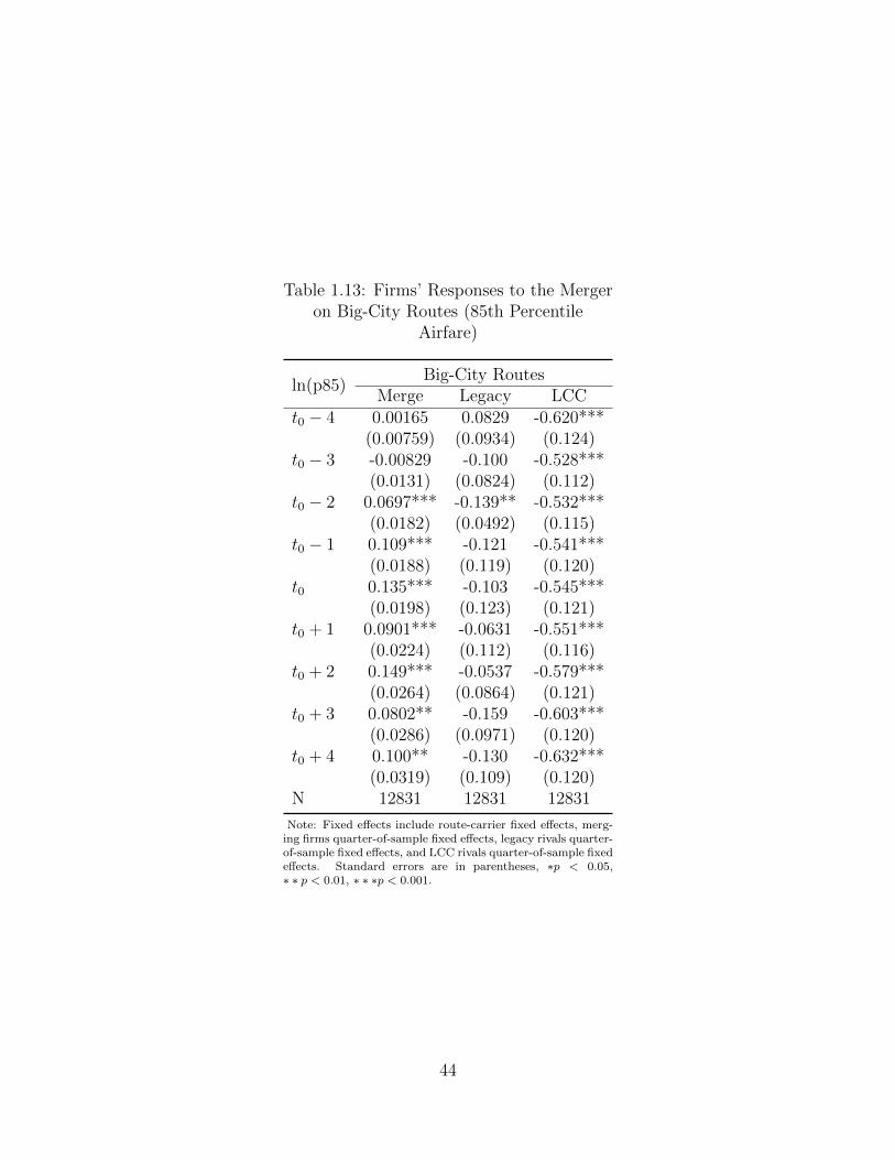
Table 1.13: Firms’ Responses to the Mergeron Big-City Routes (85th Percentile

Airfare)

ln(p85)Big-City Routes

Merge Legacy LCCt0 − 4 0.00165 0.0829 -0.620***

(0.00759) (0.0934) (0.124)t0 − 3 -0.00829 -0.100 -0.528***

(0.0131) (0.0824) (0.112)t0 − 2 0.0697*** -0.139** -0.532***

(0.0182) (0.0492) (0.115)t0 − 1 0.109*** -0.121 -0.541***

(0.0188) (0.119) (0.120)t0 0.135*** -0.103 -0.545***

(0.0198) (0.123) (0.121)t0 + 1 0.0901*** -0.0631 -0.551***

(0.0224) (0.112) (0.116)t0 + 2 0.149*** -0.0537 -0.579***

(0.0264) (0.0864) (0.121)t0 + 3 0.0802** -0.159 -0.603***

(0.0286) (0.0971) (0.120)t0 + 4 0.100** -0.130 -0.632***

(0.0319) (0.109) (0.120)N 12831 12831 12831

Note: Fixed effects include route-carrier fixed effects, merg-ing firms quarter-of-sample fixed effects, legacy rivals quarter-of-sample fixed effects, and LCC rivals quarter-of-sample fixedeffects. Standard errors are in parentheses, ∗p < 0.05,∗ ∗ p < 0.01, ∗ ∗ ∗p < 0.001.

44

Table 1.14: Firms’ Responses inCapacity on Leisure Routes (Seats)

ln(seats)Leisure Routes

Merge Legacy LCCt0 − 4 0.125 -0.0612 0.0694

(0.244) (0.0820) (0.0620)t0 − 3 0.278 -0.0808 0.0201

(0.357) (0.0951) (0.0649)t0 − 2 0.404 -0.222* -0.0480

(0.414) (0.105) (0.0854)t0 − 1 0.492 -0.0354 0.193*

(0.477) (0.125) (0.0843)t0 0.328 -0.114 0.167

(0.450) (0.147) (0.0855)t0 + 1 0.497 -0.140 0.0959

(0.591) (0.136) (0.0740)t0 + 2 0.869 -0.235 0.0266

(0.843) (0.157) (0.0971)t0 + 3 1.032 -0.259 0.210*

(1.016) (0.149) (0.0825)t0 + 4 0.863 -0.198 0.181

(0.960) (0.150) (0.0960)N 2143 2143 2143


45

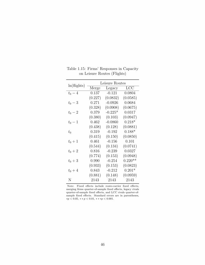
Table 1.15: Firms’ Responses in Capacityon Leisure Routes (Flights)

ln(flights)Leisure Routes

Merge Legacy LCCt0 − 4 0.137 -0.121 0.0804

(0.227) (0.0832) (0.0585)t0 − 3 0.271 -0.0926 0.0684

(0.328) (0.0908) (0.0675)t0 − 2 0.379 -0.225* 0.0317

(0.380) (0.103) (0.0947)t0 − 1 0.462 -0.0860 0.218*

(0.438) (0.128) (0.0881)t0 0.319 -0.192 0.188*

(0.415) (0.150) (0.0850)t0 + 1 0.461 -0.156 0.101

(0.544) (0.134) (0.0741)t0 + 2 0.816 -0.239 0.0327

(0.774) (0.153) (0.0948)t0 + 3 0.990 -0.254 0.220**

(0.933) (0.153) (0.0823)t0 + 4 0.843 -0.212 0.201*

(0.881) (0.148) (0.0959)N 2143 2143 2143


46

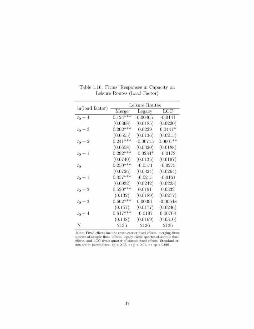
Table 1.16: Firms’ Responses in Capacity onLeisure Routes (Load Factor)

ln(load factor)Leisure Routes

Merge Legacy LCCt0 − 4 0.124*** 0.00465 -0.0141

(0.0368) (0.0185) (0.0220)t0 − 3 0.202*** 0.0229 0.0441*

(0.0555) (0.0136) (0.0215)t0 − 2 0.241*** -0.00715 0.0601**

(0.0658) (0.0320) (0.0188)t0 − 1 0.292*** -0.0284* -0.0172

(0.0740) (0.0135) (0.0197)t0 0.250*** -0.0571 -0.0275

(0.0726) (0.0324) (0.0264)t0 + 1 0.357*** -0.0215 -0.0161

(0.0932) (0.0242) (0.0223)t0 + 2 0.520*** 0.0191 0.0332

(0.132) (0.0189) (0.0277)t0 + 3 0.662*** 0.00391 -0.00648

(0.157) (0.0177) (0.0246)t0 + 4 0.617*** -0.0197 0.00708

(0.148) (0.0169) (0.0310)N 2136 2136 2136

Note: Fixed effects include route-carrier fixed effects, merging firmsquarter-of-sample fixed effects, legacy rivals quarter-of-sample fixedeffects, and LCC rivals quarter-of-sample fixed effects. Standard er-rors are in parentheses, ∗p < 0.05, ∗ ∗ p < 0.01, ∗ ∗ ∗p < 0.001.

47

Table 1.17: Firms’ Responses in Capacityon Big-City Routes (Seats)

ln(seats)Big-City Routes

Merge Legacy LCCt0 − 4 -0.0371 0.121*** 0.137*

(0.0749) (0.0346) (0.0678)t0 − 3 -0.190 -0.0442 -0.123

(0.117) (0.0832) (0.0795)t0 − 2 -0.355* -0.191** -0.256**

(0.142) (0.0588) (0.0848)t0 − 1 -0.288 0.0304 0.0599

(0.161) (0.106) (0.100)t0 -0.201 0.113 0.0322

(0.149) (0.0962) (0.145)t0 + 1 -0.294 -0.00209 -0.157

(0.194) (0.0897) (0.160)t0 + 2 -0.534 -0.131 -0.327*

(0.278) (0.104) (0.152)t0 + 3 -0.452 -0.0604 -0.0670

(0.331) (0.0789) (0.200)t0 + 4 -0.416 0.0283 0.145

(0.315) (0.0758) (0.128)N 3659 3659 3659


48

Table 1.18: Firms’ Responses in Capacity onBig-City Routes (Flights)

ln(flights)Big-City Routes

Merge Legacy LCCt0 − 4 -0.0596 0.0389 0.125

(0.0690) (0.0365) (0.0666)t0 − 3 -0.223* -0.0778 -0.0874

(0.108) (0.0793) (0.0813)t0 − 2 -0.375** -0.199*** -0.200*

(0.133) (0.0560) (0.0959)t0 − 1 -0.324* -0.0284 0.0614

(0.150) (0.109) (0.102)t0 -0.242 0.0205 0.0252

(0.138) (0.0988) (0.142)t0 + 1 -0.340 -0.0296 -0.162

(0.179) (0.0873) (0.161)t0 + 2 -0.588* -0.156 -0.325*

(0.256) (0.0978) (0.151)t0 + 3 -0.518 -0.0814 -0.0810

(0.305) (0.0828) (0.205)t0 + 4 -0.474 -0.0348 0.130

(0.291) (0.0800) (0.123)N 3659 3659 3659

Note: Fixed effects include route-carrier fixed effects, mergingfirms quarter-of-sample fixed effects, legacy rivals quarter-of-sample fixed effects, and LCC rivals quarter-of-sample fixedeffects. Standard errors are in parentheses, ∗p < 0.05, ∗ ∗ p <0.01, ∗ ∗ ∗p < 0.001.

49

Table 1.19: Firms’ Responses in Capacity onBig-City Routes (Load Factor)

ln(load factor)Big-City Routes

Merge Legacy LCCt0 − 4 -0.00154 0.0391* 0.0213

(0.0108) (0.0182) (0.0226)t0 − 3 -0.0692*** 0.0323** 0.0326

(0.0157) (0.0112) (0.0205)t0 − 2 -0.118*** -0.00845 -0.0155

(0.0187) (0.0122) (0.0191)t0 − 1 -0.0377 -0.000683 -0.00476

(0.0211) (0.0125) (0.0201)t0 -0.0363 0.0220 0.0236

(0.0199) (0.0199) (0.0277)t0 + 1 -0.104*** -0.00104 -0.0400

(0.0258) (0.0213) (0.0231)t0 + 2 -0.192*** -0.0113 -0.0122

(0.0391) (0.0162) (0.0293)t0 + 3 -0.116** 0.0238 0.000921

(0.0439) (0.0158) (0.0242)t0 + 4 -0.0972* 0.0372* 0.0677*

(0.0418) (0.0146) (0.0327)N 3644 3644 3644

Note: Fixed effects include route-carrier fixed effects, merging firmsquarter-of-sample fixed effects, legacy rivals quarter-of-sample fixed ef-fects, and LCC rivals quarter-of-sample fixed effects. Standard errors arein parentheses, ∗p < 0.05, ∗ ∗ p < 0.01, ∗ ∗ ∗p < 0.001.

50

Table 1.20: Summary Statistics of Leisure Markets with DifferentMarket Shares of LCC Rivals

VariableLeisure Routes

Merge Legacy LCCMarket Share (LCC<0.5) 0.2978 0.5758 0.1077

(0.2706) (0.2795) (0.1415)Average Airfare (LCC<0.5) 253.3678 260.7447 184.6252

(100.4246) (108.9356) (48.6968)Market Share (LCC>0.5) 0.0651 0.1253 0.8061

(0.085) (0.1049) (0.1383)Average Airfare (LCC>0.5) 183.976 194.2192 173.3181

(36.0475) (47.3703) (36.786)

Note: Standard deviations are in parentheses, LCC¡0.5(¿0.5) denotes the type of market withLCC rivals total market share less (greater) than 0.5 on leisure overlapping routes.

51

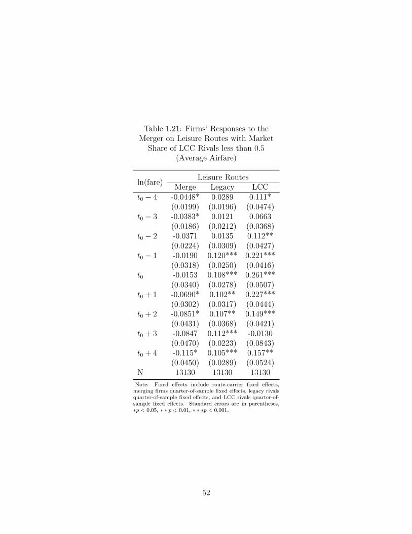
Table 1.21: Firms’ Responses to theMerger on Leisure Routes with Market

Share of LCC Rivals less than 0.5(Average Airfare)


Merge Legacy LCCt0 − 4 -0.0448* 0.0289 0.111*

(0.0199) (0.0196) (0.0474)t0 − 3 -0.0383* 0.0121 0.0663

(0.0186) (0.0212) (0.0368)t0 − 2 -0.0371 0.0135 0.112**

(0.0224) (0.0309) (0.0427)t0 − 1 -0.0190 0.120*** 0.221***

(0.0318) (0.0250) (0.0416)t0 -0.0153 0.108*** 0.261***

(0.0340) (0.0278) (0.0507)t0 + 1 -0.0690* 0.102** 0.227***

(0.0302) (0.0317) (0.0444)t0 + 2 -0.0851* 0.107** 0.149***

(0.0431) (0.0368) (0.0421)t0 + 3 -0.0847 0.112*** -0.0130

(0.0470) (0.0223) (0.0843)t0 + 4 -0.115* 0.105*** 0.157**

(0.0450) (0.0289) (0.0524)N 13130 13130 13130


52

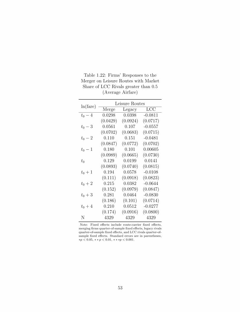
Table 1.22: Firms’ Responses to theMerger on Leisure Routes with MarketShare of LCC Rivals greater than 0.5

(Average Airfare)


Merge Legacy LCCt0 − 4 0.0298 0.0398 -0.0811

(0.0429) (0.0924) (0.0717)t0 − 3 0.0561 0.107 -0.0557

(0.0702) (0.0683) (0.0715)t0 − 2 0.110 0.151 -0.0481

(0.0847) (0.0772) (0.0702)t0 − 1 0.180 0.101 0.00605

(0.0989) (0.0665) (0.0730)t0 0.129 0.0199 0.0141

(0.0893) (0.0740) (0.0815)t0 + 1 0.194 0.0578 -0.0108

(0.111) (0.0918) (0.0823)t0 + 2 0.215 0.0382 -0.0644

(0.152) (0.0979) (0.0847)t0 + 3 0.281 0.0464 -0.0830

(0.186) (0.101) (0.0714)t0 + 4 0.210 0.0512 -0.0277

(0.174) (0.0916) (0.0800)N 4329 4329 4329


53

Chapter 2

Multimarket Contact and Price

Dispersion

2.1 Introduction

Well-developed industries often have firms competing against each other in

multiple markets. This multimarket contact is a concern for both academic and

government economists due to the issue of mutual forbearance; when firms hesitate

to apply aggressive competitive strategies in one market for fear of retaliation in

other markets in which they compete. Restrained behaviors of overlapping firms due

to multimarket contact could facilitate tacit collusion, such as setting higher prices

or price discriminating across consumer groups.

Given the potential for multimarket contact to reduce competition, many stud-

ies have investigated how multimarket contact affects price levels.1 However, no the-

oretical or empirical literature exists on the topic of how such firms adjust prices for

different consumer groups when multimarket contact intensifies. In this paper, I pro-

vide a new theoretical model to predict how a firm’s price dispersion across consumer

1These studies span a variety of industries, including Evans and Kessides (1994), Jans and Rosen-baum (1997), Parker and Roller (1997), Waldfogel and Wulf (2006), among others.

54

groups changes when firms become cooperative due to an increase in contact. The

model predictions are tested and confirmed using data from the airline industry.

Previous work suggests that competition can either increase or reduce the

degree of price dispersion. Using data from the U.S. airline industry, Borenstein

and Rose (1994) demonstrate a positive effect of competition on price dispersion,

while Gerardi and Shapiro (2009) find a negative effect. Similarly, the magnitude

of price dispersion or price discrimination can be either enhanced or weakened by

an increase in multimarket contact. More specifically, my theoretical model posits

two consumer groups (e.g., business travelers and leisure travelers) that may have

different sensitivities to purchase lower-fare tickets from a rival carrier (cross-price

elasticity). In this model environment, it is possible that price dispersion could be

smaller as firms overlap more. Suppose that business travelers are highly brand-loyal

and leisure travelers are easily attracted by cheap tickets. When multimarket contact

intensifies and firms begin pricing more cooperatively, firms would like to increase

prices more in the previously competitive leisure traveler market than in the less

competitive business traveler market. However, if the difference in the sensitivities

between the two consumer groups falls, business travelers are attracted to the low fares

as much as the leisure travelers are. When firms face greater multimarket contact and

they start colluding, the restriction on firms’ ability to price discriminate consumer

groups is loosened. Thus, firms increase the fares more for business travelers than for

leisure travelers and price dispersion tends to be larger.

Furthermore, as the market moves toward perfect competition, prices are set

close to the marginal cost and both consumer groups are sensitive to the rival firms’

lower prices. This leads to a diminished distinction of sensitivity (cross-price elas-

ticity) between business travelers and leisure travelers to purchase a rival’s low-fare

tickets. In a competitive market, higher multimarket contact could have a more

55

significant positive effect on price dispersion than in a non-competitive market.

Using airline data from the 1000 largest routes in the U.S., I test my theoretical

predictions by applying two panel data estimation approaches: ordinary least squares

(OLS) and quantile regression (QR). These empirical models specify how multimarket

contact affects price dispersion with carrier-route fixed effects and time fixed effects.

In the OLS estimation, I perform three comparisons: competitive markets versus con-

centrated markets (or less competitive markets), short hauls versus more competitive

long hauls, and legacy carriers versus low-cost carriers (LCCs). Consistent with the

theoretical predictions, when other carriers enter 10% more routes where a carrier

services, price dispersion increases by 3.05% if this carrier is in a competitive market,

2.33% if this carrier services long haul flights, and 2.07% if this carrier is an LCC.

Their comparison categories, however, exhibit no significant effects from multimarket

contact.

Both price dispersion measures (dependent variables), the Gini log-odds ratio

and fare deviation (the log value of passenger-weighted standard deviation), are not

normally distributed. This characteristic of the data indicates that it is necessary

to use the QR method. Moreover, different quantiles of price dispersion could show

various degrees of competition or collusion. As predicted by the theoretical model,

the results of QR reveal heterogeneous effects of multimarket contact among carriers.

For the 20% of observations (a carrier on a route) with the highest price dispersion, an

increase in multimarket contact significantly increases price dispersion. For the other

80% of observations, multimarket contact has no effect or a slightly negative effect

on price dispersion. More specifically, along the distribution of dependent variables,

when multimarket contact intensifies, the upper quantiles (i.e., carriers on specific

routes with high price dispersion in each quarter) experience significantly positive

effects on price dispersion. However, the middle quantiles (i.e., carriers with price

56

dispersion around the medians in each quarter) show significantly negative effects.

The bottom quantiles (i.e., carriers with low price dispersion in each quarter) seem

to exhibit no effects.

This paper builds on the extensive literature on competition and multimarket

contact. Much research has provided consistent findings that intermarket contact

is associated with higher prices (Evans and Kessides, 1994; Singal, 1996; Jans and

Rosenbaum, 1997; Parker and Roller, 1997; Busse, 2000; Waldfogel and Wulf, 2006;

Bilotkach, 2011; Miller, 2010). Using airline data, Ciliberto and Williams (2014) fill in

the gap of whether this positive correlation between prices and multimarket contact

is explained by collusive behavior. They empirically demonstrate that multimarket

contact facilitates tacit collusion among airlines. However, to my knowledge, no paper

has looked at the effects of contact among firms across markets on price dispersion

or price discrimination.

This study provides both a theoretical and an empirical setting for testing the

effects of multimarket contact on price dispersion or price discrimination. The empiri-

cal analysis gives results consistent with the predictions of the theoretical model. The

cross-price elasticity and the difference in the cross-price elasticities across consumer

groups play an important role in determining the impact of multimarket contact on

price dispersion. This is consistent with the findings of Ciliberto and Williams (2014),

who show that the cross-price elasticity is the mechanism by which multimarket con-

tact influences equilibrium price levels. However, their study does not consider how

price dispersion is influenced by multimarket contact through the cross-price elasticity

or the difference in the cross-price elasticities across consumer groups.

The organization of this paper is as follows. Section 2 presents the theoretical

model. The data and measurement of variables are provided in Section 3. Section 4

and 5 illustrate empirical models and empirical analysis. Section 6 concludes.

57

2.2 Theoretical Model

Economic theory makes predictions for how the degree of competition in a

market affects a firm’s price dispersion and price discrimination. However, there is no

explicit model to derive how the degree of collusion or connection among firms affects

price dispersion and price discrimination. In this section, based on the work of Stole

(2007) regarding the best-response symmetry in price games, I propose a theoretical

model illustrating the change in price dispersion as the probability of collusion varies

in a market.

Consider duopolists, j = a, b, in one market with two types of consumers, type

1 and type 2. Type 1 is the high type and type 2 is the low type. These two consumer

types have different demand elasticities. Type 1 consumer demand is less elastic than

that of type 2 because type 1 is more brand-loyal. Firms are able to distinguish

between these two types of consumers with some restrictions on products, such as

advance-purchase requirements and nonrefundable low-price goods. Each firm offers

products to both types of consumers and produces the products with a constant

marginal cost of c per unit. Demand for firm j’s output in the market depends

upon the prices offered by each firm for consumer type i : qji (pai , p

bi). Following Stole

(2007), I assume that these demand functions are symmetric across firms, which

are symmetric to permuting indices a and b. Thus, qi(pi) ≡ qai (pi, pi) ≡ qbi (pi, pi).

Therefore, the market elasticity of demand for consumer type i 2 can be derived as

εmi = − piqi(p)

q′i(p).

2The demand is a firm’s residual demand.

58

Moreover, firm a’s own-price elasticity of demand for consumer type i is

εai (pai , p

bi) = − pi

qai (pai , p

bi)

∂qai (pai , p

bi)

∂pi.

At the symmetric prices pi = pai = pbi , the above equation can be simplified to

εai (pai , p

bi) = − pi

qi(pi)q′i(pi) +

piqai (pi)

∂qai (pi, pi)

∂pbi.

This equation can be rewritten as

εai = εmi + εa−crossi .

Similarly, firm b’s own-price elasticity of demand for consumer type i is

εbi = εmi + εb−crossi ,

where εj−crossi > 0 is the cross-price elasticity of demand at symmetric prices pi.

Hence, the firm’s own-price elasticity of demand for consumer type i in a market can

be decomposed into two parts: the market elasticity and the cross-price elasticity.

The market elasticity measures the sensitivity of the type i consumer to buying the

outside option instead of consuming the good of either firm a or b. Here, the con-

sumer type is assumed to be predetermined and would not change due to product

restrictions imposed by firms. In addition, the cross-price elasticity measures the type

i consumer’s sensitivity to purchasing the rival’s product.

In the symmetric price equilibrium, the non-cooperative duopolists will set

prices across consumer types such that

pj−noni − cpj−noni

=1

εmi + εj−crossi

,

59

while cooperative duopolists acting as a monopolist will choose prices across consumer

types such that

pj−coopi − cpj−coopi

=1

εmi,

where εm1 < εm2 and εj−cross1 ≤ εj−cross2 . When firms are not cooperative, firm j’s price

markup dispersion across different types of consumers in a market can be written as

pj1 − cpj1

− pj2 − cpj2

=pj1 − p

j2

pj1pj2

c =1

εm1 + εj−cross1

− 1

εm2 + εj−cross2

.

When firms are cooperative, firm j’s price markup dispersion is

pj1 − cpj1

− pj2 − cpj2

=pj1 − p

j2

pj1pj2

c =1

εm1− 1

εm2.

When the probability of collusion is high and firms move from non-cooperative to

cooperative, the elasticities can be utilized to derive the change in price dispersion 3

(pj−coop1 − pj−coop2 )− (pj−non1 − pj−non2 ) = (1

εm1− 1

εm2)pj−coop1 pj−coop2

c−

(1

εm1 + εj−cross1

− 1

εm2 + εj−cross2

)pj−non1 pj−non2

c.

Ciliberto and Williams (2014) demonstrate that multimarket contact (MMC)

can help facilitate tacit collusion in the airline industry. In the following empirical

analysis, the probability of collusion is represented by MMC.

If firms raise prices for both consumer types by the same amount, then price

dispersion will not be affected, and

(1

εm1− 1


c= (

1

εm1 + εj−cross1

− 1

εm2 + εj−cross2


c,

3In the empirical analysis, the Gini coefficient and fare deviation are measures of the pricedispersion. Appendix A demonstrates that price dispersion pj1 − pj2 is highly correlated with thesetwo measures.

60

1

εm1− 1

εm2= (

1

εm1 + εj−cross1

− 1

εm2 + εj−cross2


pj−coop1 pj−coop2

.

We can denotepj−non1 pj−non

2

pj−coop1 pj−coop

2

= k, and 0 < k ≤ 1. This equation can be derived as

follows

1

εm1− 1

εm2= (

1

εm1 + εj−cross1

− 1

εm2 + εj−cross2

)k,

(1− k)εm2 + εj−cross2

εm2 (εm2 + εj−cross2 )=


εm1 (εm1 + εj−cross1 ).

We can set(1−k)εm2 +εj−cross

2

εm2 (εm2 +εj−cross2 )

= A and find

εj−cross1 =(1− k)− εm1 A

A− 1εm1

= critical point.

To guarantee that firm j’s cross-price elasticity for type 1 consumers is not negative

(i.e., εj−cross1 ≥ 0), then(1−k)−εm1 AA− 1

εm1

≥ 0. It can be proven as follows that A− 1εm1

< 0,

A− 1

εm1=


εm2 (εm2 + εj−cross2 )− 1

εm1,

A− 1

εm1=

[(1− k)εm2 + εj−cross2 ]εm1 − εm2 (εm2 + εj−cross2 )

εm1 εm2 (εm2 + εj−cross2 )

,

A− 1

εm1=

[(1− k)εm1 − εm2 ]εm2 + εj−cross2 (εm1 − εm2 )


< 0,

where (1 − k)εm1 − εm2 < 0, εm1 − εm2 < 0, and εm1 εm2 (εm2 + εj−cross2 ) > 0. Therefore,

(1− k)− εm1 A ≤ 0 or A ≥ 1−kεm1

is the condition to make sure the critical point ≥ 0.

When higher MMC causes firms to collude and raise prices more for type 1

consumers than for type 2 consumers, the price dispersion will expand. This incurs

the condition for cross-price elasticity derived as follows,

(1

εm1− 1


c> (

1

εm1 + εj−cross1

− 1

εm2 + εj−cross2


c,

61

1

εm1− 1

εm2> (

1

εm1 + εj−cross1

− 1

εm2 + εj−cross2

)k,

1

εm1− k

εm1 + εj−cross1

>1

εm2− k

εm2 + εj−cross2

,


εm1 (εm1 + εj−cross1 )>


εm2 (εm2 + εj−cross2 ),


εm1 (εm1 + εj−cross1 )> A.

Since A− 1εm1

< 0, so

εj−cross1 >(1− k)− εm1 A

A− 1εm1

,

εj−cross1 > critical point.

If firms raise prices less for type 1 consumers than for type 2 consumers, the

price dispersion will decrease. Following a similar deduction,

(1

εm1− 1


c< (

1

εm1 + εj−cross1

− 1

εm2 + εj−cross2


c,

1

εm1− 1

εm2< (

1

εm1 + εj−cross1

− 1

εm2 + εj−cross2

)k,


εm1 (εm1 + εj−cross1 )<


εm2 (εm2 + εj−cross2 ),


εm1 (εm1 + εj−cross1 )< A,

εj−cross1 <(1− k)− εm1 A

A− 1εm1

,

εj−cross1 < critical point.

Based on the above analysis, the predictions of the model can be summarized

as follows:

(1) If the equality(1−k)εm2 +εj−cross

2


=(1−k)εm1 +εj−cross

1


is satisfied, then the price disper-

62

sion of firms will not change as the market moves from competitive to collusive.

(2) However, if firm j’s cross-price elasticity for the high type consumer is greater

than the critical point (i.e., critical point < εj−cross1 ≤ εj−cross2 ), which means

the difference in cross-price elasticities across consumer types is relatively small,

the price dispersion of firms will increase as the market structure changes from

competitive to collusive.

(3) If firm j’s cross-price elasticity for the high type consumer is less than the

critical point and much less than the cross-price elasticity for the low type con-

sumer (i.e., εj−cross1 < critical point < εj−cross2 ), which means the magnitude of

the cross-price elasticities across these two consumer groups is relatively large,

firm j’s price dispersion will decrease as firms become more cooperative.

It is impossible to have a scenario where εj−cross1 ≤ εj−cross2 ≤ critical point.

The proof is as follows. We assume

εj−cross2 ≤ critical point,

εj−cross2 ≤ (1− k)− εm1 AA− 1

εm1

,

where A− 1εm1

< 0. Thus,

εj−cross2 (A− 1

εm1) ≥ (1− k)− εm1 A,

A(εm1 + εj−cross2 )− εj−cross2

εm1≥ 1− k.

Substituting A into the above equation,

[(1− k)εm2 + εj−cross2 ](εm1 + εj−cross2 )

εm2 (εm2 + εj−cross2 )− εj−cross2

εm1≥ 1− k,

63

[(1− k)εm2 + εj−cross2 ](εm1 + εj−cross2 )εm1 − εm2 (εm2 + εj−cross2 )εj−cross2


≥ 1− k,

where the denominator is greater than zero. Thus, the equation is transformed to

[(1−k)εm2 +εj−cross2 ](εm1 +εj−cross2 )εm1 −εm2 (εm2 +εj−cross2 )εj−cross2 ≥ (1−k)εm1 εm2 (εm2 +εj−cross2 ),

(1− k)εm1 εm2 (εm1 − εm2 ) + (εj−cross2 )2(εm1 − εm2 ) + εj−cross2 [(εm1 )2 − (εm2 )2] ≥ 0,

where the left-hand side is less than zero due to εm1 < εm2 . So the scenario where

εj−cross1 ≤ εj−cross2 ≤ critical point violates the assumption εm1 < εm2 .

The change in a firm’s price dispersion as the market structure varies depends

upon the difference in the cross-price elasticities across the high and low type con-

sumers in the market. If this difference is relatively large, firms in an oligopolistic

market would already take advantage of this differential when they compete and the

price dispersion would be smaller after the market becomes collusive. On the other

hand, if this difference is relatively small, firms could not use much of the price disper-

sion and price discrimination strategies when they are not cooperative. Nevertheless,

the change in the market structure plays an important role in increasing the price

dispersion. Ciliberto and Williams (2014) also demonstrate the importance of the

cross-price elasticity in determining the impact of multimarket contact on equilib-

rium fare levels. However, they show no evidence of how the cross-price elasticity

or the difference in the cross-price elasticities across consumer groups affects price

dispersion.

Furthermore, if the cross-price elasticities of the high and low type consumers

are assumed to be the same, it can be derived that the price dispersion is a decreasing

convex function over the cross-price elasticities of consumers in a market. This is

64

shown by

f(εj−cross) = (1

εm1 + εj−cross− 1

εm2 + εj−cross)p1p2

c,

where εj−cross = εj−cross1 = εj−cross2 . The first and second derivatives with respect to

εj−cross are

∂f(εj−cross)

∂εj−cross=p1p2

c[(εm2 + εj−cross)−2 − (εm1 + εj−cross)−2]+

1

c(

1


εm2 + εj−cross)(

∂p1

∂εj−crossp2 +

∂p2

∂εj−crossp1) < 0,

since εm1 < εm2 , and ∂pi∂εj−cross < 0.

∂2f(εj−cross)

∂(εj−cross)2=

2p1p2

c[(εm1 + εj−cross)−3 − (εm2 + εj−cross)−3]+

2

c(

∂p1

∂εj−crossp2 +

∂p2

∂εj−crossp1)[(εm2 + εj−cross)−2 − (εm1 + εj−cross)−2]+

1

c(

1


εm2 + εj−cross)(

∂2p1

∂(εj−cross)2p2+

2∂p1

∂εj−cross∂p2

∂εj−cross+

∂2p2

∂(εj−cross)2p1) > 0,

since εm1 < εm2 , ∂pi∂εj−cross < 0, and ∂2pi

∂(εj−cross)2> 0. This relationship is shown in the

following graph.

65

Figure 2.1: Price Dispersion is a Convex Function over Cross-price Elasticity

Note: In fact, the price is also a diminishing convex function of the cross-price elasticity and has

a similar curve. Specifically, for high type consumers (type 1 consumers), this function decreases

faster over the cross-price elasticity than for low type consumers (type 2 consumers).

As shown in Figure 2.1, the dispersion in prices charged by a firm across various

consumer groups decreases as the cross-price elasticity εj−cross increases. When the

market becomes monopolistic or cooperative (i.e., εj−cross ≈ 0), price dispersion will

reach the maximum ( 1εm1− 1

εm2)1c

at point A. However, if the market moves toward

perfectly competitive (i.e., εj−cross ≈ ∞), prices will be close to the marginal cost

for each consumer group and the price differential across groups will be negligible.

Besides extreme scenarios, this figure also illustrates two moderate cases of cross-price

elasticity, εB < εC . Point C indicates a more competitive market or a firm with more

aggressive price competition, such as low-cost carriers in the airline industry, relative

to that of point B. Thus, as the probability of tacit collusion rises due to a tight

interconnection among firms, the increase in price dispersion will be greater and more

significant for firms at point C than firms at point B (i.e., AF<AE). This analysis

reconciles with that of the magnitude between the cross-price elasticities of the high

and low type consumers in a market. As the competition becomes fiercer, a firm’s

66

cross-price elasticities of both high and low type consumers will be larger, but the

cross-price elasticity difference between these two consumer groups could be smaller.

This is because price competition forces firms to set prices close to the marginal

cost for both types of consumers. The consumers’ cross-price elasticities increase in

competition, while their market elasticities of demand will be stable regardless of

competitive status.

To test the significant effects of a change in market structure due to multi-

market contact in more competitive situations, the empirical analysis compares com-

petitive markets versus concentrated markets (or less competitive markets), short

hauls versus long hauls, and legacy carriers versus low-cost carriers. It can be pre-

dicted that competitive markets, long hauls (which are more competitive than short

hauls), and LCCs will show more significant effects than their comparison categories

of concentrated markets, short hauls, and legacy carriers.

2.3 Data and Measurement of Variables

The data source for this paper is the Airline Origin and Destination Survey

(DB1B) published by the U.S. Department of Transportation. The DB1B database

is a 10% quarterly sample of all domestic tickets issued by U.S. reporting airlines,

including information on origin, destination and connecting airports, marketing car-

riers, operating carriers, year, quarter, fare, and the number of passengers paying that

fare.4 My study focuses on domestic, direct, and coach-class airline tickets for the

4I applied several common filters often used in the airline economics literature to clean the dataand construct a comparable dataset. Only domestic direct flights are included, which encompassesboth nonstop flights and flights in which there is a stop but no change of airplane. Directionalityis suppressed. A roundtrip itinerary is split into two observations, and the fare is divided by two.Open-jaw itineraries (where a roundtrip passenger does not return to the origin city) are dropped.Observations with fares of questionable magnitude are dropped, and bulk fares are eliminated aswell. Fares greater than five times the DOT’s Standard Industry Fare Level (SIFL) are also excluded.I also dropped all fares that are less than $20 for a one-way trip. Only coach-class tickets are kept.

67

year 2017:Q1-Q4. This time period was chosen because several airline mergers and

acquisitions happened in the past 10 years. This caused the airline industry to enter

a tightly oligopolistic era and these few remaining firms kept expanding their network

by opening new routes. The inter-market connection could play an important role in

this scenario.

For each quarter, I include data on only the 1000 largest routes in terms of

passenger volume. Following the approach of Evans and Kessides (1994), I eliminate

airlines that service less than 10 of the largest 1000 routes and less than 1 percent of

passengers on a route. Monopoly routes are dropped due to no contact for carriers

on these routes. Carriers reporting only one level of fares are eliminated since there

is no price differential across consumers. After the data cleaning process, the final

dataset contains 16254 observations from 1073 routes5 and 11 airlines6 for the year

2017.

The unit of observation is a carrier within a route in a given quarter of the

year. Two major dependent variables are constructed to capture the level of price dis-

persion: the Gini coefficient and fare deviation. Following the method of Borenstein

and Rose (1994), the formula for the Gini coefficient can be computed as follows7

GINI = 1− 2× {N∑i=1

[farei × PAXi

total revenue× (1−

i∑j=1

PAXj

total PAX)]},

where N is the number of different fare level tickets reported by a carrier on a route

Coupon types indicating foreign carrier flying between 2 U.S. points are dropped. To deal with theissue of code sharing, I dropped flights including a change of ticketing carriers and flights in whichthe operating and ticketing carriers are different.

5The identity of the 1000 largest routes changes from quarter to quarter, so more than 1000routes are included in the final sample.

6These 11 airlines include 5 legacy airlines and 6 low-cost carriers (LCC). Legacy airlines areAlaska, American, Delta, Hawaiian, and United. LCCs are Frontier, Allegiant, Spirit, Sun Country,Virgin, Southwest.

7There could be a typo or mistake in their formula, so I rewrote it here.

68

in a given quarter, farei is the reported fare for the ith ticket, and PAXi is the

reported number of passengers traveling at that fare.

The log value of passenger-weighted standard deviation of fares for a carrier

on a route (hereafter fare deviation) is calculated by the following equation

LogSD = ln [(1

N − 1

N∑i=1

ωi(farei − fare))12 ],

where N and farei are the same as above, ωi is the passenger weight for the ith ticket,

and fare is the passenger-weighted average fare, calculated as fare = 1N

∑Ni=1 ωifarei.

In addition, following the approaches of Evans and Kessides (1994) and Baum

and Korn (1996), I construct both route-level and carrier-level multimarket contact

indexes to indicate the probability of collusion among firms. The route-level index

captures the extent of multimarket contact among the airlines that service the route,

which is an average number of contact for all carriers on the route. The carrier-level

index of a carrier on a route measures the average market domain overlap with other

carriers, which defines how important other competitors are to this carrier. Both

indexes are based on pairwise comparisons of airline contact. The formulas are as

follows

akl =n∑j=1

DkjDlj,

AvgRouteContactj =1

[fj(fj − 1)/2]

m∑k=1

m∑l=k+1

aklDkjDlj,

Route− LevelMMCj =AvgRouteContactj

1000,

Carrier − LevelMMClj =

∑mk 6=l aklDkjDlj

(∑n

j Dlj)(fj − 1),

where the time subscript is dropped for now. n and m represent the number of routes

and airlines, respectively, Dkj(Dlj) is a dummy variable that equals one if airline

69

k(l) offers flights on route j and zero otherwise, akl measures the number of routes

serviced by both airline k and l concurrently, and fj is the number of carriers on

route j. Another variable I use in my analysis is the negative log of the Herfindahl-

Hirschman index (− ln (HHI)), which captures the market competition or market

concentration of a route.

Table 2.1 presents the statistics of these five variables from the data sample,

and Figures 2.2 and 2.3 plot the histograms and quantiles of both price dispersion

variables, the Gini coefficient and fare deviation. Different from the other three

variables (Route-level MMC, Carrier-level MMC, and ln(HHI)), the distributions of

both the Gini coefficient and fare deviation are not likely to be normal. 75% of

observations with Gini coefficient are less than 0.31 and these with fare deviation

are smaller than 2.52. This characteristic of the dependent variables shows it is

inappropriate to merely use OLS estimation for panel data. This is because mean

regression masks this heterogeneity. Thus, I will apply QR in the empirical analysis

to capture how multimarket contact influences price dispersion differently with the

change in price dispersion.

In addition to this feature of the data, Gerardi and Shapiro (2009) demonstrate

that an increase in competition over time along a route results in a decrease in price

dispersion in the airline industry. Their conclusion is consistent with textbook theory,

which states that as the market moves toward perfect competition, the dispersion in

prices charged by an individual firm in a given market will fall. In the QR approach,

different quantiles of the response variable could show various degrees of competition

or collusion. The ambiguous effects of multimarket contact can be identified based

on different level of market competition.

Table 2.2 partitions all the carriers into subsamples by the 30th, 60th, and

90th percentiles of carrier-level multimarket contact index. The means and medians

70

of the Gini coefficient seem to be increasing as the carrier-level MMC of firms rises.

However, this pattern is inconsistent with the trend shown in the fare deviation, which

presents negligible growth in price dispersion as multimarket contact enhances. The

price dispersion even drops to its smallest value in the most interdependent group.

This suggests that the relationship between multimarket contact and price dispersion

may not be linear, as shown in the former theoretical predictions.

2.4 Empirical Models

According to the theoretical predictions, multimarket contact can either in-

crease or decrease the price dispersion as the market moves from competitive to

collusive. This section explores empirically how multimarket contact influences price

dispersion with the U.S. airline market.

The analysis follows the estimation strategy in Gerardi and Shapiro (2009), but

adds a multimarket contact variable to the regression model. The basic specification

is as follows:

ycrt = α + β1MMCcrt + β2(− ln (HHIrt)) +Xrtθ + γt + ϑcr + εcrt,

where ycrt represents a firm’s price dispersion. This is expressed by the Gini log-odds

ratio, given by Gloddcrt = ln [GINIcrt/(1−GINIcrt)], and the fare deviation for carrier

c on route r in time t. There are two fixed effects included here: time fixed effects

and carrier-route fixed effects, denoted by γt and ϑcr, respectively. − ln (HHIrt) is

the negative value of the natural log of route r’s Herfindahl-Hirschman Index in time

t. The key variable of interest, MMCcrt is the carrier-level multimarket contact

for carrier c on route r in time t. Higher levels of multimarket contact have been

shown theoretically and empirically to increase the probability of collusion for the

71

carrier on that route. Xrt controls for route characteristics and costs including the

nonstop distance, the slot-controlled airport,8 the competition from Southwest, the

competition from other LCCs, the market share of Southwest, and the market share

of other LCCs. In OLS estimation, the standard errors are clustered at the carrier-

route level to account for heteroscedasticity and correlation across observations for a

particular carrier-route combination over time.

I apply two estimation strategies for panel data: OLS and QR. Given that

the effects of multimarket contact can depend upon the characteristics of the market,

the average effects obtained from OLS estimation may be somewhat misleading. QR

estimation helps better explore how the impact of multimarket contact differs across

markets.

The QR model characterizes various quantiles along the price dispersion dis-

tribution, which consists of these price dispersions of firms. This model is given by:

ycrt = β1τMMCcrt + β2τ (− ln (HHIrt)) + γtτ + ϑcrτ + εcrtτ,

where 0 < τ < 1 indicates the price dispersion below the quantile τ . The conditional

quantile function τ [·] is specified as:

τ [ycrt|MMCcrt,− ln (HHIrt), γtτ , ϑcrτ ] = β1τMMCcrt+β2τ (− ln (HHIrt))+γtτ +ϑcrτ ,

where each estimated coefficient measures the effect of the corresponding regressors

on ycrt at the τth quantile of ycrt. For instance, a coefficient on MMCcrt at τ = 0.5

measures the effect of an increment of carrier-level multimarket contact on price

dispersion at the 50th quantile of the conditional price dispersion distribution.

8The Federal Aviation Administration (FAA) uses runway slots to limit scheduled air traffic atcertain capacity constrained airports. These airports include John F. Kennedy International Airport(JFK), LaGuardia Airport (LGA), and Ronald Reagan National Airport (DCA).

72

I adopt the method introduced by Powell (2016), which is a QR approach

for panel data with nonadditive fixed effects. The traditional method with additive

fixed effects changes the structural quantile function and the conditional outcome

distribution. However, this approach with nonadditive fixed effects maintains the

nonseparable disturbance term commonly associated with quantile estimation. A

further advantage is that this approach permits an unspecified distribution for the

data generating process of the outcome variable.

2.5 Empirical Analysis

Both OLS and QR results are presented and compared in this section. For

the QR, inspection of the draw sequences confirms that the coefficients converge after

5000 iterations. The results indicate that the algorithm can recover the parameters

sufficiently. I run the estimation with 10000 iterations for each quantile and discard

the first 1000 runs as a burn-in. I use the last 9000 iterations in an MCMC (Markov

Chain Monte Carlo) simulation to estimate the model’s parameters.

2.5.1 OLS Panel Estimations

Table 2.3 contains estimation results for both price and price dispersion mod-

els. Before discussing the focus of this study, the multimarket contact effect, I will

look at the control variables. Consistent with previous work, the effects of an increase

in competition, measured by the market concentration -ln(HHI), on price and price

dispersion are negative and significant. Four variables are included to represent the

effects of LCCs: the presence of Southwest and other LCCs, and the market share of

Southwest and other LCCs. In contrast with the work of Brueckner et al. (2013), only

the presence of Southwest reduces fares and fare dispersions. The presence of other

73

LCCs is generally associated with higher price levels and greater price dispersion.

As shown in Table 2.3, consistent with the conclusions of Evans and Kessides

(1994), multimarket contact increases carriers’ passenger-weighted average fares. As

contact increases by one standard deviation (0.1298), the fare increases by about

2.54%9. Additionally, the price dispersion regressions reveal that routes with greater

MMC have significantly higher price dispersion on average.

To begin investigating differences across markets in the effects of multimarket

contact on price dispersion, I decompose the whole sample by market competition,

route nonstop distance, and carrier type. When the market moves toward perfect

competition, the dispersion in prices charged by an individual firm in a given market

will fall. This indicates that the difference between the cross-price elasticities of the

high and low type consumers becomes smaller when competition is stronger. Gerardi

and Shapiro (2009) mention that there is a positive correlation between the distance

of a route and the degree of competition. In my data, I find the same pattern as

well. As the log value of nonstop distance moves from less than the 25th percentile

to greater than the 75th percentile, the average number of effective competitors rises

from 4.1 to 6.1.10 The reason for distinguishing legacy carriers and LCCs is that they

have different business models and pricing strategies. Legacy carriers adopt the hub-

and-spoke network, while LCCs use the point-to-point operating practice. Usually,

the average fares of LCCs are lower than those of legacy carriers. In my dataset, the

average and median fares of LCCs are around $166, but about $230 for legacy carriers.

This suggests that there could be a higher proportion of price elastic consumers as

more LCCs compete in the market.

9exp(0.179)-1)*0.129810Gerardi and Shapiro (2009) use the effect of route density to explain the source of this positive

relationship between competition and distance. With a few exceptions, large cities in the UnitedStates tend to be relatively far from each other. The demand for air travel increases with thepopulations of endpoints, so more carriers would like to provide flight services.

74

Table 2.4 shows the mean and median price dispersion by market, distance,

and carrier. For both market and distance categories, I use the median values of

Herfindahl-Hirschman Index and logarithm of nonstop distance as the criteria to

decompose the whole sample into either competitive markets (HHI<median) or con-

centrated markets (HHI>median), and either short hauls (distance<median) or long

hauls (distance> median).11 Both concentrated markets and short haul flights tend

to have larger price dispersion than competitive markets and long haul flights. How-

ever, legacy carriers and LCCs show a negligible difference in price dispersion. This

might suggest that as the airline industry evolves, LCCs gain the ability to engage

in price dispersion or price discrimination to some extent, while the legacy carriers

always have this ability. In the following subsections, I compare the carrier-level

multimarket contact effects on price dispersion in these partitioned samples.

2.5.1.1 Competitive Markets VS Concentrated Markets

The first column of Table 2.5 shows the regression results for competitive

markets with HHI less than its median value in the sample. The coefficient of MMC

is significantly positive. In the second column, we see an insignificant coefficient

of MMC for the concentrated markets. Thus, the more contacts for a carrier with

other firms in competitive markets, the higher the price dispersion than a carrier

in concentrated markets. The obvious disparity of the MMC coefficients in these

two estimations is likely a consequence of the larger cross-price elasticities of both

high (business travelers or brand-loyal customers) and low (leisure travelers or non-

brand-loyal customers) type consumers in competitive markets than in concentrated

markets, which is shown in Figure 2.1. With an increase in multimarket contact,

11This median value threshold is not critical, as the summary statistics (Table 2.4) and laterregressions (Tables 2.5 and 2.6) are not sensitive to it.

75

a firm in the comparatively competitive market increases its price dispersion more

significantly as the market structure moves toward more cooperative. Additionally,

according to prediction (2) of the theoretical model, the positive effects of MMC in

competitive markets also indicate that the differential between cross-price elasticities

of high and low type consumers should be relatively small.

Table 2.5 also shows that the effects of negative market competition and South-

west presence are stronger in concentrated markets than in competitive markets. This

makes sense due to the smaller number of competitors in concentrated markets. The

marginal effects of an increase in competition could be stronger in concentrated mar-

kets, either from the decrease in market concentration or Southwest joining in the

market.

Statistics show that the mean of the market share of other LCCs in competitive

markets is 19%, which is more than twice the average of 8% in concentrated markets.

This disparity in average market share seems to reveal that the effects of the presence

of other LCCs are stronger in competitive markets. However, at the levels of average

market share for both types of markets, the net impact of other LCCs is 0.112 for

competitive markets and 0.0913 for concentrated markets. These two net affects are

fairly similar.

2.5.1.2 Short Hauls VS Long Hauls

The results of short hauls versus long hauls are shown in Table 2.6. The

pattern of multimarket contact effects on price dispersion is similar to the one with

competitive markets versus concentrated markets. This is because routes with longer

distances tend to be relatively more competitive than routes with shorter distances.

120.0925 ∗ 0.19 + 0.0830130.474 ∗ 0.08 + 0.0490

76

Thus, as shown in Figure 2.1, the cross-price elasticities for both high and low type

consumers in long haul markets are likely to be greater than in short haul markets.

This distinction of cross-price elasticity of demand across short and long hauls leads

to the different effects of MMC as markets switch to a more collusive structure. Like

the results in the competitive markets versus concentrated markets, the significantly

positive effects of MMC in long hauls imply the difference in cross-price elasticity

across high and low type consumers is relatively small according to the prediction

(2).

As seen in Table 2.6, the competition effects measured by -ln(HHI) are similar

on both short and long haul routes. An incremental increase in -ln(HHI) decreases

price dispersion by around 10%.

In contrast to the results in Table 2.5, although markets with long distance

flights are more competitive than markets with short distance flights, competition

from Southwest demonstrates more robust effects in long haul flights than in short

haul flights. At the average levels of Southwest market share, that is, 43% for short

hauls and 23% for long hauls, the net competitive effects from Southwest are even

much stronger in long haul markets. However, the coefficients of the presence of other

LCCs are close in both short and long haul regressions. As the market shares of other

LCCs rise to the average levels, which are 13% for short haul routes and 14% for long

haul routes, the net effects of other LCCs are still roughly close at 0.09 for short hauls

and 0.07 for long hauls.

As illustrated in Tables 2.5 and 2.6, both coefficients of Southwest market

share and other LCCs market share present a pattern of more substantial effects in

the less competitive (short haul) routes than in the competitive (long haul) routes.

The market share of LCCs could be related to the fraction of price-sensitive consumers

to some extent, due to their low-fare strategy. Thus, the fraction of brand-loyal or

77

high type consumers falls as this market share grows. According to switching cost

theory (Klemperer, 1987a; Hastings, 2004), under price competition, firms’ optimal

price increases in the share of its brand-loyal consumers and its competitors’ share

of brand-loyal consumers, but decreases in the share of non-brand-loyal consumers.

Therefore, as the market share of LCCs rises, rival firms tend to drop fares for both

price-insensitive and price-conscious travelers. But if the optimal fares for price-

insensitive consumers drop less than the fares for price-conscious consumers, then the

price dispersion could expand. This effect can be more clear in a market with a more

distinct difference in the cross-price elasticity for the high and low type consumers,

as in concentrated markets and short hauls markets.

2.5.1.3 Legacy Carriers VS Low Cost Carriers

The results for legacy carriers versus LCCs are reported in Table 2.7. Col-

umn (1) only uses the observations of legacy carriers as a subsample, while column

(2) just includes the LCCs observations as a subsample. Similar to the above two

comparisons, the pattern of the coefficients of the MMC variable in both columns

is consistent with the theoretical predictions illustrated in Figure 2.1. Multimarket

contact significantly increases the price dispersion of LCCs, but shows no significant

effects on the price dispersion of legacy carriers. LCCs, unlike legacy carriers, ap-

ply cheap pricing strategies with no-frills passenger experience and charge plenty of

fees for such luxuries as additional bags or extra legroom. This low-fare policy likely

implies that consumers buying tickets from an LCC rather than a legacy carrier are

attracted mostly by cheap fares. This means that the cross-price elasticity of demand

for LCCs is relatively higher than that of legacy carriers. Consequently, when firms

engage in tacit collusion, the change in price dispersion is larger and more significant

for LCCs than legacy carriers. Additionally, the incremental effects of MMC on the

78

price dispersion of LCCs indicate the small difference between cross-price elasticities

of high and low type consumers, consistent with the prediction (2).

As seen in Table 2.7, both coefficients of ln(HHI) in the legacy carriers and

LCCs regressions are around -12%. Southwest has a larger competitive effect on LCCs

(i.e., -0.284) than on legacy carriers (i.e., -0.153), and the net competitive effect is

stronger (i.e., -0.357 on LCCs and -0.0959 on legacy carriers) at the average level of

Southwest market share of 33%. This trend suggests that Southwest competes more

aggressively with other LCCs than with legacy carriers. In contrast, the presence of

other LCCs displays positive effects on the price dispersion of both LCCs and legacy

carriers. When the market share of other LCCs rises to its average level of 14%, the

net effects on legacy carriers increase to 0.09 while the net effects on LCCs decrease

to 0.06.

An incremental increase in the market share of LCCs shrinks the dispersion of

prices charged by an LCC, but expands the dispersion of prices charged by a legacy

carrier. The market share of Southwest illustrates a similar magnitude for both

legacy carriers and LCCs. However, the market share of other LCCs has a positive

effect on legacy carriers that is more than double its negative effect on LCCs. As

previously mentioned, the market share of LCCs could be related to the fraction of

price-sensitive consumers. The conclusions here are consistent with the above results,

which are explained by the switching cost theory that rival carriers tend to drop

optimal fares for price-sensitive travelers as the market share of LCCs rises. Usually,

legacy carriers have more differentiated consumer groups than LCCs. Thus, when

the percentage of price-elastic consumers increases, a legacy carrier is able to keep its

optimal fares for the high type consumers somewhat stable, but reduces fares for the

low types. On the other hand, an LCC may have to drop fares more for high type

consumers, leading to a reduction in price dispersion.

79

2.5.2 Quantile Regressions

Quantile regression estimates for the full sample of the Gini log-odds ratio and

fare deviation at a select few values of τ(0.10, 0.25, 0.50, 0.75, 0.90) are presented

in Tables 2.8 and 2.9. Different from the OLS panel estimates in Table 3, MMC

shows significantly negative and positive effects as well as zero effects as the quantile

of dependent variables moves. It seems that the mean effects of MMC (0.128 in the

Gini log-odds ratio regression and 0.271 in the fare deviation regression) reported by

the OLS estimation reflect the effects observed for the 80th quantile of both dependent

variables’ distributions. About 20% of the observations (a carrier on a route) with the

highest price dispersion show that multimarket contact significantly increases price

dispersion, but for the other 80% of the observations, multimarket contact displays

no effect or a slightly negative effect on price dispersion. However, the effect of an

increase in competition (-ln(HHI)) on price dispersion is greatly consistent with the

mean effect presented by the OLS regression.

Figures 2.4 and 2.5 plot all 99 point estimates of MMC and -ln(HHI) by

quantiles of the Gini log-odds ratio and fare deviation from τ = 0.01 to τ = 0.99.

These estimates of -ln(HHI) consistently move around the OLS estimate. However,

the point estimates of MMC by quantiles display a distinctive pattern in both plots.

In the bottom quantiles of the Gini log-odds ratio (τ = 0− 0.30) and fare deviation

(τ = 0 − 0.39), multimarket contact shows no effects on price dispersion. In the

middle quantiles (τ = 0.30 − 0.6 for the Gini log-odds ratio and τ = 0.39 − 0.54 &

τ = 0.68 − 0.77 for the fare deviation), the effects are negative. The effects change

to positive when moving to the upper quantiles, at τ = 0.80 − 0.90 for the Gini

log-odds ratio and τ = 0.84 − 0.95 for the fare deviation. This pattern of MMC

point estimates illustrates the potential for heterogeneous effects as predicted by the

80

theoretical model.

By applying the method of Powell (2016), the quantile regressions control for

individual fixed effects and time fixed effects with nonadditive fixed effects. However,

the individual fixed effects are not included or even estimated in this de-meaning

approach. Thus, to recover those dependent variables corresponding to the bottom,

middle, and upper quantiles, I check the unconditional distributions of both the Gini

log-odds ratio and fare deviation in each quarter. By comparing the unconditional

quantiles with the quantiles conditional on regressors, I find that the gap could be

considered negligible. Therefore, it is reasonable to utilize the unconditional distri-

butions.

Based on these recovered quantiles of the dependent variables from their un-

conditional distributions in each quarter, I calculate the statistics of several variables.

Table 10 presents the statistics for the Gini coefficient, fare deviation, carrier-level

MMC, HHI, nonstop distance, market share of LCCs, and presence of LCC by the

bottom, middle, and upper quantile ranges. On average, as the quantile range moves

from bottom to middle and to upper, both price dispersion variables (the Gini coef-

ficient and fare deviation) increase.

In Table 2.10, both means and medians of LCC market share and presence

of LCC are lower for middle quantiles compared to other two quantile ranges, which

to some extent indicates that firms have a small fraction of price-sensitive consumers

and weak competition from LCCs. This may reveal that firms in the middle quantile

range face high and low type consumer groups with a larger difference in their cross-

price elasticities. Without the strong price competition from LCCs, firms in the

middle quantile range are capable of price discriminating consumers with certain

ticket restrictions. According to prediction (3) of the theoretical model, the price

dispersion of firms will decrease as the market moves from competitive toward tacitly

81

collusive if the critical point is in the middle of cross-price elasticity of high and low

type consumers, which explains the case for the middle quantiles.

For both bottom and upper quantiles in Table 2.10, besides the high market

share of LCCs and high presence of LCCs, there seems to be no other significant

pattern. The difference in cross-price elasticity across consumer groups in the bottom

quantile range probably satisfies the equality condition stated in prediction (1). Thus,

when firms become more cooperative, there could be no significant effects of MMC.

However, this effect turns to be positive if the difference in cross-price elasticity across

consumer groups is small as in prediction (2), which corresponds to the results for

the upper quantiles.

2.6 Conclusions

This paper examines price dispersion of firms across consumer types when the

probability of collusion, represented by the carrier-level multimarket contact, becomes

higher. The theoretical model constructed in this study predicts effects of multimar-

ket contact. Specifically, multimarket contact could help the price dispersion of a

firm if the difference in cross-price elasticities of the high and low type consumers is

relatively small. However, multimarket contact could hurt the price dispersion of a

firm if this difference is relatively large. In addition, if the cross-price elasticities of

the high and low type consumers are assumed to be the same, the price dispersion is

proved to be a decreasing convex function of the cross-price elasticity. Therefore, as

the cross-price elasticity or competition increases, price dispersion is smaller. Nev-

ertheless, the change in price dispersion could be larger and more significant for a

more competitive market or a firm when firms become cooperative due to intensified

multimarket contact.

82

The empirical analyses presented by the OLS panel estimations and QR are

consistent with the predictions of the theoretical model. I perform three comparisons

that decompose markets or carriers of different types: competitive markets versus

concentrated markets, short hauls versus long hauls, and legacy carriers versus low-

cost carriers. The results show significant positive effects of multimarket contact

in the cases of competitive markets, long haul flights, and low-cost carriers. These

three groups are believed to have relatively larger cross-price elasticities across both

the high and low type consumers than their comparison categories of concentrated

markets, short haul flights, and legacy carriers. Moreover, the QR for panel data

with nonadditive fixed effects provide further evidence on the heterogeneous effects

of multimarket contact. These effects vary from zero effects to negative effects to

positive effects as the quantile of the dependent variables (the Gini log-odds ratio

and fare deviation) moves from low quantiles to high quantiles. The reasons for

this pattern are explained by the differences in the cross-price elasticity across the

consumer types, as illustrated in the predictions of the theoretical model.

In addition to the significant heterogeneous effects of multimarket contact on

price dispersion, there is also surprising evidence shown by competition from low-cost

carriers, including Southwest and other LCCs. Consistent with the work of Morrison

(2001), Goolsbee and Syverson (2008), and Brueckner et al. (2013), the presence

of Southwest still presents strong competitive effects on fare dispersion. However,

inconsistent with the studies of Dresner et al. (1996) and Brueckner et al. (2013), the

presence of other LCCs reveals significant noncompetitive effects on price dispersion.

Furthermore, the effects of LCC market share on price dispersion, a topic not studied

by previous papers, show opposite coefficients for legacy carriers and LCCs. As the

LCC market share rises, the fare dispersion of a legacy carrier expands, while the

price dispersion of an LCC shrinks. Future research on the source of these various

83

effects by LCCs is necessary.

84

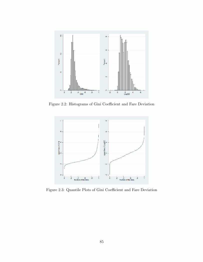
Figure 2.2: Histograms of Gini Coefficient and Fare Deviation

Figure 2.3: Quantile Plots of Gini Coefficient and Fare Deviation

85

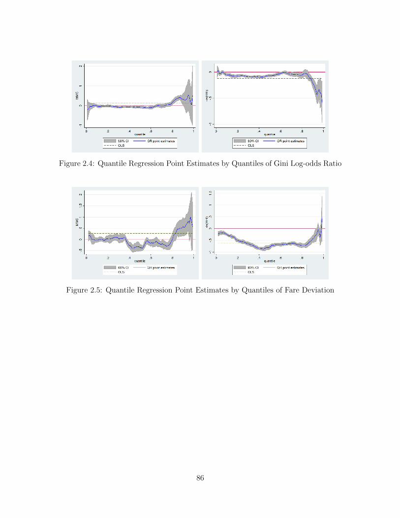
Figure 2.4: Quantile Regression Point Estimates by Quantiles of Gini Log-odds Ratio

Figure 2.5: Quantile Regression Point Estimates by Quantiles of Fare Deviation

86

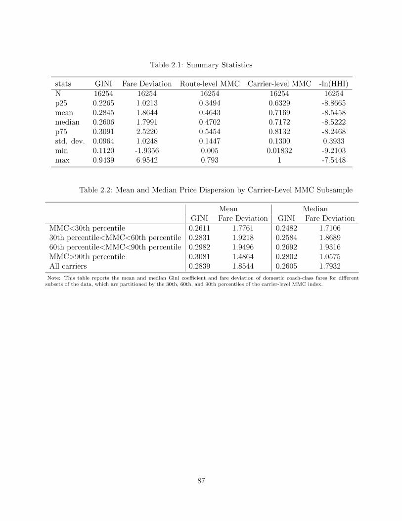
Table 2.1: Summary Statistics

stats GINI Fare Deviation Route-level MMC Carrier-level MMC -ln(HHI)N 16254 16254 16254 16254 16254p25 0.2265 1.0213 0.3494 0.6329 -8.8665mean 0.2845 1.8644 0.4643 0.7169 -8.5458median 0.2606 1.7991 0.4702 0.7172 -8.5222p75 0.3091 2.5220 0.5454 0.8132 -8.2468std. dev. 0.0964 1.0248 0.1447 0.1300 0.3933min 0.1120 -1.9356 0.005 0.01832 -9.2103max 0.9439 6.9542 0.793 1 -7.5448

Table 2.2: Mean and Median Price Dispersion by Carrier-Level MMC Subsample

Mean MedianGINI Fare Deviation GINI Fare Deviation

MMC<30th percentile 0.2611 1.7761 0.2482 1.710630th percentile<MMC<60th percentile 0.2831 1.9218 0.2584 1.868960th percentile<MMC<90th percentile 0.2982 1.9496 0.2692 1.9316MMC>90th percentile 0.3081 1.4864 0.2802 1.0575All carriers 0.2839 1.8544 0.2605 1.7932

Note: This table reports the mean and median Gini coefficient and fare deviation of domestic coach-class fares for differentsubsets of the data, which are partitioned by the 30th, 60th, and 90th percentiles of the carrier-level MMC index.

87

Table 2.3: OLS Panel Estimates of Price and PriceDispersion Models

(1) (2) (3)ln (fare) LogSD Glodd

crt

MMC 0.179*** 0.271*** 0.128**(0.0447) (0.100) (0.0646)

-ln(HHI) -0.0947*** -0.614*** -0.121***(0.0197) (0.0519) (0.0285)

Southwest Mkt Share 0.0837* 0.178 0.0458(0.0475) (0.138) (0.0734)

Southwest -0.142*** -0.227*** -0.179***(0.0447) (0.0836) (0.0460)

Other LCC Mkt share -0.0356 0.167 0.187***(0.0427) (0.122) (0.0656)

Other LCC 0.0332*** 0.0988*** 0.0552***(0.00988) (0.0236) (0.0155)

Nonstop Distance 0.696*** 1.684*** 1.083***(0.170) (0.505) (0.280)

Constant -0.469 -15.24*** -9.529***(1.207) (3.571) (1.980)

Observations 16254 16254 16254

Note: Fixed effects include route-carrier fixed effects and time fixed effects. Standarderrors in parentheses, ∗p < 0.1, ∗ ∗ p < 0.05, ∗ ∗ ∗p < 0.01.

88

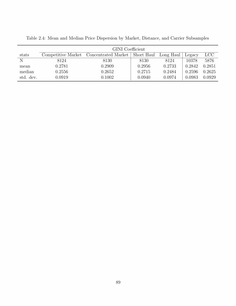
Table 2.4: Mean and Median Price Dispersion by Market, Distance, and Carrier Subsamples

GINI Coefficientstats Competitive Market Concentrated Market Short Haul Long Haul Legacy LCCN 8124 8130 8130 8124 10378 5876mean 0.2781 0.2909 0.2956 0.2733 0.2842 0.2851median 0.2556 0.2652 0.2715 0.2484 0.2596 0.2625std. dev. 0.0919 0.1002 0.0940 0.0974 0.0983 0.0929

89

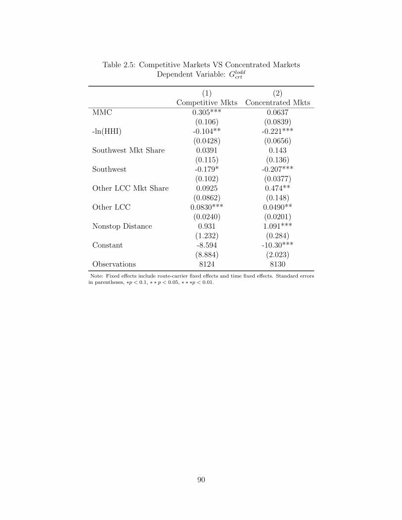
Table 2.5: Competitive Markets VS Concentrated MarketsDependent Variable: Glodd

crt

(1) (2)Competitive Mkts Concentrated Mkts

MMC 0.305*** 0.0637(0.106) (0.0839)

-ln(HHI) -0.104** -0.221***(0.0428) (0.0656)

Southwest Mkt Share 0.0391 0.143(0.115) (0.136)

Southwest -0.179* -0.207***(0.102) (0.0377)

Other LCC Mkt Share 0.0925 0.474**(0.0862) (0.148)

Other LCC 0.0830*** 0.0490**(0.0240) (0.0201)

Nonstop Distance 0.931 1.091***(1.232) (0.284)

Constant -8.594 -10.30***(8.884) (2.023)

Observations 8124 8130

Note: Fixed effects include route-carrier fixed effects and time fixed effects. Standard errorsin parentheses, ∗p < 0.1, ∗ ∗ p < 0.05, ∗ ∗ ∗p < 0.01.

90

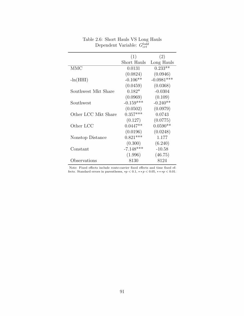
Table 2.6: Short Hauls VS Long HaulsDependent Variable: Glodd

crt

(1) (2)Short Hauls Long Hauls

MMC 0.0131 0.233**(0.0824) (0.0946)

-ln(HHI) -0.106** -0.0981***(0.0459) (0.0368)

Southwest Mkt Share 0.182* -0.0304(0.0969) (0.109)

Southwest -0.159*** -0.240**(0.0502) (0.0979)

Other LCC Mkt Share 0.357*** 0.0743(0.127) (0.0775)

Other LCC 0.0447** 0.0590**(0.0196) (0.0248)

Nonstop Distance 0.821*** 1.177(0.300) (6.240)

Constant -7.148*** -10.58(1.996) (46.75)


Note: Fixed effects include route-carrier fixed effects and time fixed ef-fects. Standard errors in parentheses, ∗p < 0.1, ∗ ∗ p < 0.05, ∗ ∗ ∗p < 0.01.

91

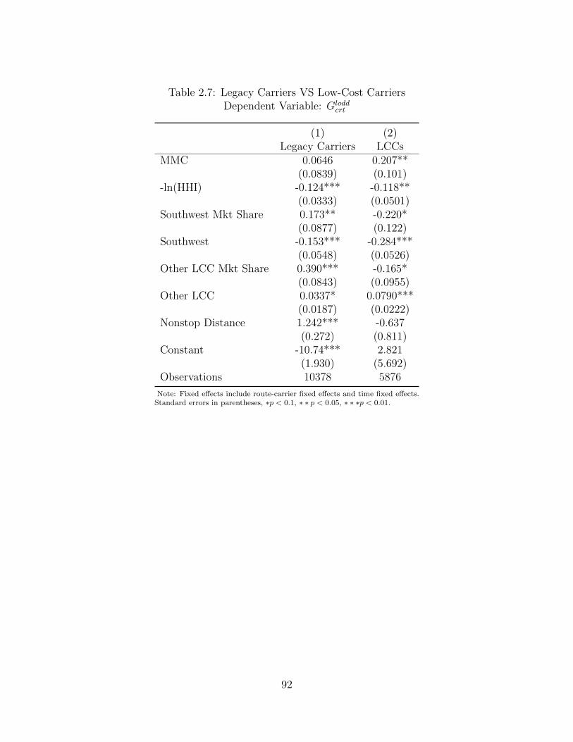
Table 2.7: Legacy Carriers VS Low-Cost CarriersDependent Variable: Glodd

crt

(1) (2)Legacy Carriers LCCs

MMC 0.0646 0.207**(0.0839) (0.101)

-ln(HHI) -0.124*** -0.118**(0.0333) (0.0501)

Southwest Mkt Share 0.173** -0.220*(0.0877) (0.122)

Southwest -0.153*** -0.284***(0.0548) (0.0526)

Other LCC Mkt Share 0.390*** -0.165*(0.0843) (0.0955)

Other LCC 0.0337* 0.0790***(0.0187) (0.0222)

Nonstop Distance 1.242*** -0.637(0.272) (0.811)

Constant -10.74*** 2.821(1.930) (5.692)


Note: Fixed effects include route-carrier fixed effects and time fixed effects.Standard errors in parentheses, ∗p < 0.1, ∗ ∗ p < 0.05, ∗ ∗ ∗p < 0.01.

92

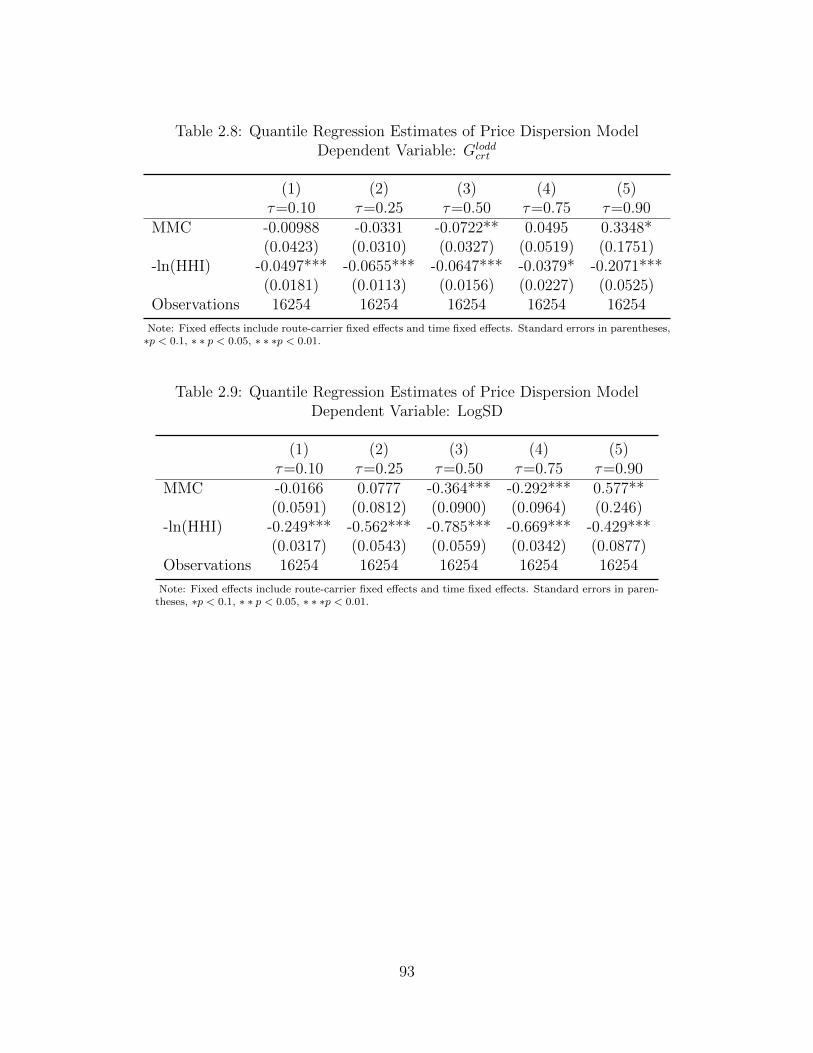
Table 2.8: Quantile Regression Estimates of Price Dispersion ModelDependent Variable: Glodd

crt

(1) (2) (3) (4) (5)τ=0.10 τ=0.25 τ=0.50 τ=0.75 τ=0.90

MMC -0.00988 -0.0331 -0.0722** 0.0495 0.3348*(0.0423) (0.0310) (0.0327) (0.0519) (0.1751)

-ln(HHI) -0.0497*** -0.0655*** -0.0647*** -0.0379* -0.2071***(0.0181) (0.0113) (0.0156) (0.0227) (0.0525)

Observations 16254 16254 16254 16254 16254

Note: Fixed effects include route-carrier fixed effects and time fixed effects. Standard errors in parentheses,∗p < 0.1, ∗ ∗ p < 0.05, ∗ ∗ ∗p < 0.01.

Table 2.9: Quantile Regression Estimates of Price Dispersion ModelDependent Variable: LogSD

(1) (2) (3) (4) (5)τ=0.10 τ=0.25 τ=0.50 τ=0.75 τ=0.90

MMC -0.0166 0.0777 -0.364*** -0.292*** 0.577**(0.0591) (0.0812) (0.0900) (0.0964) (0.246)

-ln(HHI) -0.249*** -0.562*** -0.785*** -0.669*** -0.429***(0.0317) (0.0543) (0.0559) (0.0342) (0.0877)

Observations 16254 16254 16254 16254 16254

Note: Fixed effects include route-carrier fixed effects and time fixed effects. Standard errors in paren-theses, ∗p < 0.1, ∗ ∗ p < 0.05, ∗ ∗ ∗p < 0.01.

93

Table 2.10: Statistics by Quantile Ranges of Gloddcrt and LogSD

Gloddcrt stats GINI Fare Deviation MMC HHI Nonstop Distance Mkt Share of LCC Presence of LCC

Bottom Quantiles

N 4877 4877 4877 4877 4877 4877 4877mean 0.2081 1.4543 0.6902 5222.0150 7.2068 0.4131 0.3771

median 0.2116 1.4008 0.6873 4796.6750 7.3271 0.3533 0std. dev. 0.0228 0.6242 0.1273 2027.1390 0.5620 0.3341 0.4847

Middle Quantiles

N 4876 4876 4876 4876 4876 4876 4876mean 0.2542 1.6157 0.7111 5633.0290 6.9852 0.4744 0.3037

median 0.2531 1.6412 0.7095 5161.0060 6.9745 0.4321 0std. dev. 0.0170 0.7618 0.1298 2141.6080 0.5553 0.3470 0.4599

Upper Quantiles

N 1626 1626 1626 1626 1626 1626 1626mean 0.3518 2.3034 0.7505 5595.3020 6.9085 0.5007 0.4729

median 0.3509 2.6245 0.7556 5037.6760 6.9012 0.4679 0std. dev. 0.0279 1.1021 0.1280 2162.4890 0.5504 0.3446 0.4994

LogSD

Bottom Quantiles

N 6338 6338 6338 6338 6338 6338 6338mean 0.2527 0.8644 0.7238 5378.9120 6.8834 0.4844 0.5497

median 0.2451 0.8743 0.7144 4889.5400 6.9048 0.4462 1std. dev. 0.0544 0.3422 0.1423 2193.3860 0.5861 0.3382 0.4976

Middle Quantiles

N 4946 4946 4946 4946 4946 4946 4946mean 0.2623 2.0764 0.7019 5443.9880 7.1504 0.4434 0.2608

median 0.2529 2.2405 0.7040 4983.4710 7.1763 0.3851 0std. dev. 0.0626 0.4219 0.1211 2050.5310 0.5219 0.3412 0.4391

Upper Quantiles

N 1785 1785 1785 1785 1785 1785 1785mean 0.3689 3.2316 0.7330 6331.1990 6.9741 0.4815 0.2308

median 0.3482 3.1998 0.7476 5855.2500 6.9460 0.4368 0std. dev. 0.0981 0.2475 0.1245 2305.0140 0.6033 0.3807 0.4215

94

Appendices

95

Appendix A Relationship between Price Disper-

sion and the Gini Coefficient and Fare

Deviation

This appendix tests whether the price dispersion (pj1 − pj2) used in the theo-

retical model is positively related to the price dispersion variables for the empirical

analysis, the Gini coefficient and fare deviation (LogSD). Two measures are used to

calculate the price dispersion: (1) PD1=pj75 − pj25, and (2) PD2=pj90 − p

j10.The term

pj25 (pj75, pj10, pj90) is the 25th (75th, 10th, 90th) percentile fare charged by carrier j on

a route. Figure A1 shows that the distributions of both measures are similar to the

distribution of the Gini coefficient in Figure 2.2. These distributions are not normal

and have long right-tails. The pool data depict that price dispersion is positively cor-

related with the Gini coefficient and fare deviation in Figures A2 and A3. As shown

in Table A1, the price dispersion variables (PD1 and PD2) are much larger than the

Gini coefficient and fare deviation on average, so in the later regressions both PD1

and PD2 are scaled down by 1000.

The following empirical model for panel data is used to test the relationship

between the PD and Gini coefficient and fare deviation

ycrt = α + βPD + γt + ϑcr + εcrt.

This specification is similar to the model in the OLS panel estimation. The variable

ycrt is expressed by the Gini coefficient and fare deviation for carrier c on route r in

time t. There are two fixed effects included here: time fixed effects and carrier-route

fixed effects, denoted by γt and ϑcr, respectively. The variable PD includes PD1 and

PD2. The standard errors are clustered at the carrier-route level.

96

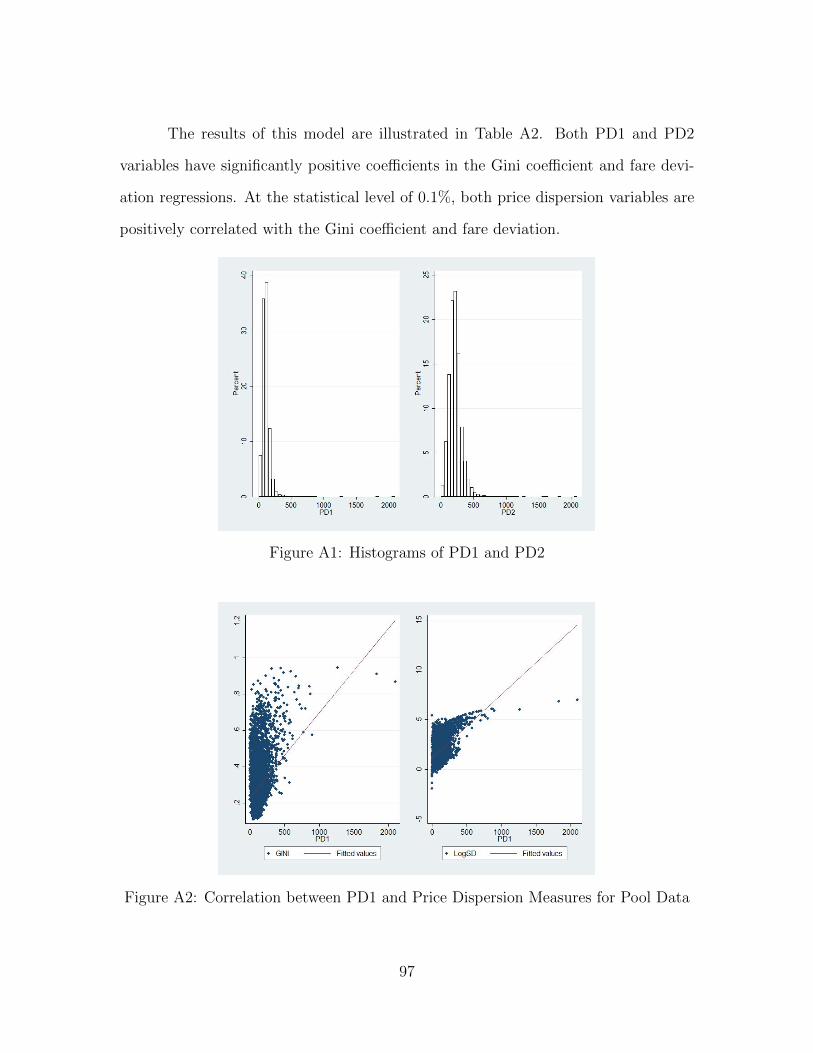
The results of this model are illustrated in Table A2. Both PD1 and PD2

variables have significantly positive coefficients in the Gini coefficient and fare devi-

ation regressions. At the statistical level of 0.1%, both price dispersion variables are

positively correlated with the Gini coefficient and fare deviation.

Figure A1: Histograms of PD1 and PD2

Figure A2: Correlation between PD1 and Price Dispersion Measures for Pool Data

97

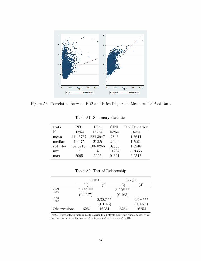
Figure A3: Correlation between PD2 and Price Dispersion Measures for Pool Data

Table A1: Summary Statistics

stats PD1 PD2 GINI Fare DeviationN 16254 16254 16254 16254mean 114.6757 224.3947 .2845 1.8644median 106.75 212.5 .2606 1.7991std. dev. 62.3216 106.0266 .09635 1.0248min .5 .5 .11204 -1.9356max 2095 2095 .94391 6.9542

Table A2: Test of Relatonship

GINI LogSD(1) (2) (3) (4)

PD11000

0.589*** 5.226***(0.0227) (0.168)

PD21000

0.302*** 3.398***(0.0143) (0.0975)

Observations 16254 16254 16254 16254

Note: Fixed effects include route-carrier fixed effects and time fixed effects. Stan-dard errors in parentheses, ∗p < 0.05, ∗ ∗ p < 0.01, ∗ ∗ ∗p < 0.001.

98

Bibliography

Baum, J. A. and Korn, H. J. (1996). Competitive dynamics of interfirm rivalry.Academy of Management journal, 39(2):255–291.

Bilotkach, V. (2011). Multimarket contact and intensity of competition: evidencefrom an airline merger. Review of Industrial Organization, 38(1):95–115.

Borenstein, S. (1990). Airline mergers, airport dominance, and market power. TheAmerican Economic Review, 80(2):400–404.

Borenstein, S. and Rose, N. L. (1994). Competition and price dispersion in the usairline industry. Journal of Political Economy, 102(4):653–683.

Brueckner, J. K., Lee, D., and Singer, E. S. (2013). Airline competition and domesticus airfares: A comprehensive reappraisal. Economics of Transportation, 2(1):1–17.

Busse, M. R. (2000). Multimarket contact and price coordination in the cellulartelephone industry. Journal of Economics & Management Strategy, 9(3):287–320.

Carlton, D. W., Israel, M. A., MacSwain, I., and Orlov, E. (2016). Are legacy airlinemergers pro-or anti-competitive? evidence from recent us airline mergers.

Ciliberto, F. and Williams, J. W. (2014). Does multimarket contact facilitate tacitcollusion? inference on conduct parameters in the airline industry. The RANDJournal of Economics, 45(4):764–791.

Dresner, M., Lin, J.-S. C., and Windle, R. (1996). The impact of low-cost carrierson airport and route competition. Journal of Transport Economics and Policy,pages 309–328.

Evans, W. N. and Kessides, I. N. (1994). Living by the golden rule: Multimar-ket contact in the us airline industry. The Quarterly Journal of Economics,109(2):341–366.

Frank, R. G. and Salkever, D. S. (1997). Generic entry and the pricing of pharma-ceuticals. Journal of Economics & Management Strategy, 6(1):75–90.

99

Gerardi, K. S. and Shapiro, A. H. (2009). Does competition reduce price dispersion?new evidence from the airline industry. Journal of Political Economy, 117(1):1–37.

Goolsbee, A. and Syverson, C. (2008). How do incumbents respond to the threat ofentry? evidence from the major airlines. The Quarterly journal of economics,123(4):1611–1633.

Hastings, J. S. (2004). Vertical relationships and competition in retail gasoline mar-kets: Empirical evidence from contract changes in southern california. The Amer-ican Economic Review, 94(1):317–328.

Hollander, A. (1987). On price-increasing entry. Economica, pages 317–324.

Huschelrath, K. and Muller, K. (2015). Market power, efficiencies, and entry evidencefrom an airline merger. Managerial and Decision Economics, 36(4):239–255.

Jain, V. (2015). What did the wave bring?: Short-term price effect of the us airlinemerger wave (2009-2012). Journal of Economic Policy and Research, 10(2):49.

Jans, I. and Rosenbaum, D. I. (1997). Multimarket contact and pricing: Evidencefrom the us cement industry. International Journal of Industrial Organization,15(3):391–412.

Kim, E. H. and Singal, V. (1993). Mergers and market power: Evidence from theairline industry. The American Economic Review, pages 549–569.

Klemperer, P. (1987a). The competitiveness of markets with switching costs. TheRAND Journal of Economics, pages 138–150.

Klemperer, P. (1987b). Markets with consumer switching costs. The quarterly journalof economics, 102(2):375–394.

Kwoka, J. and Shumilkina, E. (2010). The price effect of eliminating potential com-petition: Evidence from an airline merger. The journal of industrial economics,58(4):767–793.

Luo, D. (2014). The price effects of the delta/northwest airline merger. Review ofIndustrial Organization, 44(1):27–48.

Miller, A. R. (2010). Did the airline tariff publishing case reduce collusion? TheJournal of Law and Economics, 53(3):569–586.

Morrison, S. A. (2001). Actual, adjacent, and potential competition estimating thefull effect of southwest airlines. Journal of Transport Economics and Policy(JTEP), 35(2):239–256.

100

Parker, P. M. and Roller, L.-H. (1997). Collusive conduct in duopolies: multimar-ket contact and cross-ownership in the mobile telephone industry. The RANDJournal of Economics, pages 304–322.

Perloff, J. M. and Salop, S. C. (1985). Equilibrium with product differentiation. TheReview of Economic Studies, 52(1):107–120.

Powell, D. (2016). Quantile regression with nonadditive fixed effects. Quantile Treat-ment Effects.

Prager, R. A. and Hannan, T. H. (1998). Do substantial horizontal mergers generatesignificant price effects? evidence from the banking industry. The Journal ofIndustrial Economics, 46(4):433–452.

Prince, J. T. and Simon, D. H. (2017). The impact of mergers on quality provi-sion: Evidence from the airline industry. The Journal of Industrial Economics,65(2):336–362.

Rosenthal, R. W. (1980). A model in which an increase in the number of sellers leadsto a higher price. Econometrica: Journal of the Econometric Society, pages1575–1579.

Singal, V. (1996). Airline mergers and multimarket contact. Managerial and DecisionEconomics, pages 559–574.

Stole, L. A. (2007). Price discrimination and competition. Handbook of industrialorganization, 3:2221–2299.

Tan, K. M. (2016). Incumbent response to entry by low-cost carriers in the us airlineindustry. Southern Economic Journal, 82(3):874–892.

Waldfogel, J. and Wulf, J. (2006). Measuring the effect of multimarket contact oncompetition: Evidence from mergers following radio broadcast ownership dereg-ulation. The BE Journal of Economic Analysis & Policy, 5(1).

Weinberg, M. (2007). The price effects of horizontal mergers. Journal of CompetitionLaw and Economics, 4(2):433–447.

Whinston, M. D. and Collins, S. C. (1992). Entry and competitive structure inderegulated airline markets: an event study analysis of people express. TheRAND Journal of Economics, pages 445–462.

101

Documents

Essays on Firm Pricing Behaviors in the U.S. Airline Industry