Essays on Asymmetric Information in Financial MarketsEssays on Asymmetric Information in Financial Markets by Bradyn Mitchel Breon-Drish A dissertation submitted in partial satisfaction

Essays on Asymmetric Information in Financial Markets

by

Bradyn Mitchel Breon-Drish

A dissertation submitted in partial satisfaction of the

requirements for the degree of

Doctor of Philosophy

in

Business Administration

in the

Graduate Division

of the

University of California, Berkeley

Committee in charge:

Professor Christine Parlour, ChairProfessor Johan Walden

Professor Robert M. Anderson

Spring 2011


Copyright 2011by


1

Abstract


by


Doctor of Philosophy in Business Administration

University of California, Berkeley

Professor Christine Parlour, Chair

This dissertation studies the effects of asymmetric information and learning on asset pricesand investor decision-making. Two main themes run through the work. The first is thelinkage between investor decisions and the information used to make those decisions; that is,portfolio choices reflect the nature and quality of available information. The second theme isthe interaction between investor learning and price informativeness. The information held byindividual investors is reflected in market prices through their trading decisions, and pricesthus transmit this information to other investors.

In the first chapter, Asymmetric Information in Financial Markets: Anything Goes, Istudy a standard Grossman and Stiglitz (1980) noisy rational expectations economy, butrelax the usual assumption of the joint normality of asset payoff and supply. The primarycontribution is to characterize how the equilibrium relation between price and fundamentalsdepends on the way in which investors react to the information contained in price. My solu-tion approach dispenses with the typical “conjecture and verify” method, which allows meto analytically solve an entire class of previously intractable nonlinear models that nests thestandard model. This simple generalization provides a purely information-based channel formany common phenomena. In particular, price jumps and crashes may arise endogenously,purely due to learning effects, and observation of the net trading volume may be valuablefor investors in the economy as it can provide a refinement of the information conveyed byprice. Furthermore, the value of acquiring information may be non-monotonic in the numberof informed traders, leading to multiple equilibria in the information market. I show alsothat the relation between investor disagreement and returns is ambiguous and depends onhigher moments of the return distribution. In short, many of the standard results from noisyrational expectations models are not robust. I introduce monotone likelihood ratio condi-tions that determine the signs of the various comparative statics, which represents the firstdemonstration of the implicit importance of the MLRP in the noisy rational expectationsliterature.

In the second chapter, Do Fund Managers Make Informed Asset Allocation Decisions?,a joint work with Jacob S. Sagi, we derive a dynamic model in which mutual fund managers

2

make asset allocation decisions based on private and public information. The model pre-dicts that the portfolio market weights of better informed managers will mean revert fasterand be more variable. Conversely, portfolio weights that mean revert faster and are morevariable should have better forecasting power for expected returns. We test the model ona large dataset of US mutual fund domestic equity holdings and find evidence consistentwith the hypothesis of timing ability, especially at three- to 12-month forecasting horizons.Nevertheless, whatever timing ability may be reflected in portfolio weights does not appearto translate into higher realized returns on funds’ portfolios.

i

Contents

1 Asymmetric Information in Financial Markets: Anything Goes 11.1 Introduction . . . . . . . . . . . . . . . . . . . . . . . . . . . . . . . . . . . . 11.2 Model . . . . . . . . . . . . . . . . . . . . . . . . . . . . . . . . . . . . . . . 5

1.2.1 Equilibrium . . . . . . . . . . . . . . . . . . . . . . . . . . . . . . . . 71.3 Discussion of the monotone likelihood ratio property . . . . . . . . . . . . . 111.4 General results . . . . . . . . . . . . . . . . . . . . . . . . . . . . . . . . . . 16

1.4.1 Uninformed demand and the information content of prices . . . . . . 161.4.2 The value of observing signed volume . . . . . . . . . . . . . . . . . . 191.4.3 The value of acquiring information . . . . . . . . . . . . . . . . . . . 221.4.4 The relation between disagreement and returns . . . . . . . . . . . . 27

1.5 Conclusion . . . . . . . . . . . . . . . . . . . . . . . . . . . . . . . . . . . . . 291.6 Appendix . . . . . . . . . . . . . . . . . . . . . . . . . . . . . . . . . . . . . 31

1.6.1 Some results on single-crossing and sign-regular functions . . . . . . . 311.6.2 Proofs . . . . . . . . . . . . . . . . . . . . . . . . . . . . . . . . . . . 33

2 Do Fund Managers Make Informed Asset Allocation Decisions 462.1 Introduction . . . . . . . . . . . . . . . . . . . . . . . . . . . . . . . . . . . . 46

2.1.1 Literature review and motivation . . . . . . . . . . . . . . . . . . . . 472.1.2 Our contribution . . . . . . . . . . . . . . . . . . . . . . . . . . . . . 49

2.2 A model of optimal market timing . . . . . . . . . . . . . . . . . . . . . . . . 512.2.1 Testable predictions . . . . . . . . . . . . . . . . . . . . . . . . . . . . 55

2.3 Empirical investigation . . . . . . . . . . . . . . . . . . . . . . . . . . . . . . 562.3.1 Data . . . . . . . . . . . . . . . . . . . . . . . . . . . . . . . . . . . . 582.3.2 The market forecasting power inherent in weight dynamics . . . . . . 612.3.3 Robustness checks . . . . . . . . . . . . . . . . . . . . . . . . . . . . 63

2.4 Does successful ‘timing’ translate into higher returns? . . . . . . . . . . . . . 652.5 Conclusions . . . . . . . . . . . . . . . . . . . . . . . . . . . . . . . . . . . . 662.6 Appendix . . . . . . . . . . . . . . . . . . . . . . . . . . . . . . . . . . . . . 67

2.6.1 Proofs . . . . . . . . . . . . . . . . . . . . . . . . . . . . . . . . . . . 672.6.2 Reproducing the results from Jiang, Yao, and Yu (2007) . . . . . . . 712.6.3 Robustness of equity portfolio timing regressions . . . . . . . . . . . . 72

ii

Acknowledgments

Special thanks to my advisor Christine Parlour for continuous guidance and support, alongwith detailed comments on many drafts. Jacob Sagi provided helpful thoughts on the firstchapter in this dissertation, and is a co-author on the second chapter. I would also like tothank Robert Anderson, Nicolae Garleanu, Simon Gervais, Hayne Leland, and Johan Waldenfor discussions and comments.

1

Chapter 1

Asymmetric Information in FinancialMarkets: Anything Goes

1.1 Introduction

Since at least Hayek (1945) economists have recognized that an important role of finan-cial markets is the aggregation and transmission of information held by individual traders.There is a vast literature, both theoretical and empirical, that seeks to understand how wellprices reflect information and what frictions best explain apparent deviations from marketefficiency.1 Following this literature, I seek to explore several questions: How do tradersreact to the information in prices? Are asset prices a sufficient statistic for all public infor-mation? Are prices necessarily more informative when more traders are informed? How isdisagreement among investors reflected in prices and future returns?

Addressing the interaction between price informativeness and investor behavior presup-poses, of course, that traders have asymmetric information, for without information asym-metry there is no role for learning from price. The workhorse model for studying asymmetricinformation in (competitive) financial markets is the noisy rational expectations (RE) modelof Grossman and Stiglitz (1980), and similar ones due to Hellwig (1980) and Diamond andVerrecchia (1981).2 Unfortunately, the standard model is ill-suited for a full considerationof the questions posed above. It makes counterfactual assumptions about the distribution ofasset payoffs and supply, and it leads to overly-simplistic descriptions of investor behavior.

1Fama (1991) is a standard reference on empirical tests of market efficiency. Brunnermeier (2001) discussesthe theory.

2There is a distinct but related literature, following Kyle (1985), that studies the consequences of asym-metric information in markets in which some traders behave strategically. Other models in this vein includeAdmati and Pfleiderer (1988), Holden and Subrahmanyam (1992), and Foster and Viswanathan (1993, 1996),in which traders submit market orders, and Kyle (1989) and Bhattacharya and Spiegel (1991), in whichtraders submit demand schedules. There is also a literature, initiated by Admati (1985), that considersnoisy RE models with multiple assets.

2

In the standard model, all random variables are jointly normally distributed, and de-mand curves and asset prices are linear functions. Hence, all price observations are equallyinformative, and traders always react in the same way to changes in price. In practice, assetreturns and supply are not jointly normally distributed. Fama (1965) and Mandelbrot (1963)were among the first to make note of this fact. Kon (1984) finds that discrete mixtures ofnormal distributions better describe stock returns than either normal, Student-t, or stableParetian distributions. (Tucker (1992) reinforces this point with additional statistical tests,and Hall, Brorsen, and Irwin (1989) provide complementary evidence in the context of fu-tures markets.) Recently, nonnormality has also received much coverage in the popular pressin the context of heavy tails (see, for instance, Taleb (2007)).

In this paper, I investigate the effects of asymmetric information in a class of noisy rationalexpectations models in which I relax the standard Grossman and Stiglitz (1980) model toadmit fundamentals and supply that do not follow a normal distribution. This seeminglyminor change can have dramatic consequences for the standard results on the shape ofdemand curves (and consequently the possibility of information-based price crashes), priceinformativeness, the value of acquiring information, and the relation between disagreementand returns. The simplicity of the classic Grossman and Stiglitz (1980) economy makes it anideal setting in which to illustrate the fragility of noisy RE models. My point is strengthenedby the limited number of moving parts; more general models can be expected to provide evenricher results as they afford more degrees of freedom for constructing examples.

My primary contribution is to characterize how the relation between price and funda-mentals depends on the strength and direction in which investors react to information inprice. I provide a purely information-based channel for many common phenomena. Morespecifically, I show how price-informativeness varies with the price level and how learningeffects can cause uninformed investors to submit backward-bending demand curves, lead-ing to price “jumps” and “crashes” in response to small changes in fundamentals.3 Next, Ishow that observation of (signed) trading volume may be valuable for uninformed investorsbecause it provides a refinement of the information contained in price alone. Third, I showthat the value of information can be non-monotonic in the number of informed investorsin the economy. That is, information acquisition can be a strategic complement. Finally,I demonstrate that the relation between investor disagreement and returns depends on therelation between conditional expected returns and conditional volatility and on the skewnessof fundamentals.

In standard noisy RE models price crashes are impossible in the absence of other frictions.Demand curves of uninformed investors are downward-sloping at all prices, and because oflinearity they always respond in the same way to perturbations in price.4 As such, authors

3Strictly speaking, my model is static, so there are no changes to which traders can react. I follow theconvention of many papers in this literature, e.g., Gennotte and Leland (1990) and Barlevy and Veronesi(2003), and interpret comparative statics as approximating dynamic effects in a repeated version of themodel.

4In the multi-asset noisy RE model of Admati (1985), demand curves can be globally upward sloping.

3

modeling crashes in settings with asymmetric information often introduce context-specificfrictions. To rationalize the October 1987 crash, Gennotte and Leland (1990) introduceimperfectly anticipated hedging demand, which can cause large price reactions in response tosmall changes in fundamentals. Similarly, Romer (1993) introduces higher-order uncertaintyover the information quality of other traders. In his model, small changes in price can revealthis information quality and lead to discontinuous drops in price. Yuan (2005) considersthe effects of borrowing constraints, which make low prices less informative: uninformedinvestors have difficulty disentangling whether low price is due to a low fundamental or abinding borrowing constraint that has prevented informed from trading fully on the basis ofinformation. Similarly, Barlevy and Veronesi (2003) study a model with risk-neutral traderswho are both short-sale and borrowing constrained. My model differs from all of the above inthat I focus solely on the effect of asymmetric information with fully-rational unconstrainedinvestors. It turns out that crashes arise naturally in settings with asymmetric informationbecause, in general, different price realizations are not equally informative.

It is also difficult to reconcile the empirical evidence on the information content of tradingvolume and other market-generated statistics with standard rational expectations models.5

Typically, price is a sufficient statistic for all public information, and other market-generatedstatistics are redundant. Schneider (2009) gives a clear statement of this point, noting that“the fact that volume is helpful to an outside observer of the economy does not imply thatinvestors within the economy can learn from observing volume. If investors are rational,then it is not clear how trading volume can contain information beyond the informationthat is already incorporated into prices.” Schneider (2009) and Blume, Easley, and O’Hara(1994) introduce higher-order uncertainty and propose that volume can be informative aboutthe quality of others’ information. In my model, (signed) volume can be valuable, butthe mechanism is different. Without normality, price may not be a sufficient statistic forpublic information and in such situations, signed volume refines the uninformed investors’information set.

Following the original Grossman and Stiglitz (1980) paper, the standard intuition is thatas the number of informed investors in a market increases, it becomes easier to free-rideon their information by simply observing price. As such, the incentive for other traders toacquire information decreases–information acquisition is a strategic substitute. There is asmall recent literature investigating the opposite situation, strategic complementarity in in-formation acquisition. Barlevy and Veronesi (2000, 2008) introduce correlated fundamentalsand supply, which makes it more difficult for uninformed investors to disentangle whetherprice changes are due to fundamentals of supply. Ganguli and Yang (2009) and Manzano andVives (2010) allow investors to also observe signals about the supply. Veldkamp (2006a,b)considers a dynamic Grossman and Stiglitz (1980) model with economies of scale in the

However, as they are still linear they never bend backwards and generate crashes of the sort discussed here.5See, e.g., Karpoff (1987), Gallant, Rossi, and Tauchen (1992), and Gervais, Kaniel, and Mingelgrin

(2001) for evidence on the relation between volume and returns.

4

(competitive) information market. In such a setting, information in higher demand is sup-plied at a lower price, generating complementarities. My model generates complementaritythrough a pure information channel: when the number of informed investors increases, pricemay become more difficult to read, causing uninformed investors to submit demand curvesthat are less closely aligned with those of informed investors.

While the model allows for essentially general distributions of uncertainty for both theasset payoff and supply, one need not depart too far from normality to obtain the resultsabove. Normal mixture distributions have been proposed as an empirically plausible al-ternative to normal distributions (Kon, 1984), and as shown later, simple normal mixturespecifications can produce a rich set of examples. In the standard model, the strong uni-modality of the normal distribution implies that uninformed investors are able to learn fromprices relatively “easily” (later, I make the unimodality condition precise and describe learn-ing effects explicitly). High price is an unambiguous signal of high payoff (and vice versa),so that the informed and uninformed investors react in the same direction to a change inthe fundamental and the equilibrium price function is monotone. When the number of in-formed investors increases, the information contained in price is “more correlated” with thefundamental, and uninformed investors are able to make portfolio decisions that are closerto those of the informed and therefore better aligned with the true state. Similarly, thefact that the conditional variance of a normal random variable, given another jointly normalrandom variable, is constant implies that there are no price levels at which an uninformedinvestor learns more or less than any other price level. With more general distributions thisis not true without further restrictions on the distribution of uncertainty. I give examples ofthe above effects in Sections 1.4 below.

In order to derive the results above, I provide a tractable solution to a particular class ofnonlinear noisy rational expectations models that nests the standard model. Instead of theusual solution method of conjecturing and verifying a (linear) price function, I approach theproblem by solving a general version of the uninformed investors’ optimization problem givenan arbitrary price function and then utilize the market clearing condition to write down anequation that pins down the price as an implicit function of the primitive quantities in themodel. In principle, the technique I use would also allow for uncertainty about quantitiesother than the conditional mean of asset payoffs, such as the variance, number of informed,or risk aversion.

Other notable exceptions to the normality assumption in the literature include Ausubel(1990a,b), Peress (2004), and Vanden (2008). However, these authors must make unappeal-ing concessions and use a non-standard model setup or approximation methods. Bernardoand Judd (2000) develop a computational procedure for solving rational expectations mod-els and demonstrate the non-robustness of some results from the standard Grossman andStiglitz (1980) model. An advantage of their approach is the large class of models that ithandles, but without an explicit characterization of price, it is difficult to pin down theconditions on distributions or preferences that drive standard results. The economy of Bar-levy and Veronesi (2000, 2003) is similar to that in this paper, except that their traders

5

are risk-neutral and face a portfolio constraint, and they focus on a particular parametricdistribution for random variables. Gibbons, Holden, and Powell (2010) consider a noisyRE model of an intermediate goods market in which all random variables are uniformlydistributed and demonstrate non-robustness of some of the Grossman and Stiglitz (1980)results in their setting. DeMarzo and Skiadas (1998, 1999) study the properties a class ofeconomies that nests the non-noisy economy of Grossman (1976); they demonstrate unique-ness of Grossman’s (1976) fully-revealing linear equilibrium and give robust examples ofpartially revealing equilibria when payoffs are non-normal. Foster and Viswanathan (1993)study (linear) equilibria in the Kyle (1985) model when random variables are ellipticallydistributed, and Bagnoli, Viswanathan, and Holden (2001) derive necessary and sufficientconditions on probability distributions for existence of linear equilibria in various marketmaking models. Finally, Rochet and Vila (1994) study existence and uniqueness propertiesin a model similar to Kyle (1985) with non-normal distributions.

The rest of the paper proceeds as follows. Section 1.2 lays out the model and characterizesthe equilibrium. Section 1.3 discusses the monotone likelihood ratio property and previewsits role in many of the results in the paper. Section 1.4 lays out the general results describedabove, and Section 1.5 concludes. Section 1.6.1 collects results on sign-regular and singlecrossing functions that are used to prove some of my propositions. Proofs are relegatedto Section 1.6.2. Since my results speak to a number of different literatures, I postponeadditional detailed discussion of related papers to the sections in which I present the relevantfindings.

1.2 Model

The economy has three dates t ∈ {0, 1, 2}. At the first date, t = 0, agents choose whetherto become informed. At the second, t = 1, agents trade financial assets. At the final date,t = 2, assets make liquidating payouts. Figure 1.2 shows a timeline. There are two assets,a risky asset that has a payoff D and a risk-free asset that pays 1 and has price normalizedto 1. The risky-asset payoff D is the sum of two components µ and ε. The distribution ofthe fundamental µ has density fµ, while ε is independently distributed N(0, σ2

ε). Note thatbecause of the normal distribution for ε, the conditional distribution of D given µ is normal.

The assumption that ε has a normal distribution is not critical for my results, but itgreatly simplifies the analysis. One way to motivate this assumption is to consider thateven after the fundamental µ is known, there are a “large” number of “small” additiveand independent idiosyncratic factors that can affect the final payoff. By the central limittheorem, the sum of these disturbances will be approximately normally distributed, and onecan just as well aggregate them into a single term, namely ε. While this interpretation isplausible, I do not model it rigorously here.

To prevent fully-revealing prices, the risky asset is in random supply Z, which is inde-pendent of other random variables in the model and has density fZ . To simplify the proofs

6

? ? ?

t = 0 t = 1 t = 2

Information acquisition decision

Informed see fundamentals

Financial market opens

Agents trade competitively

Payoffs realized

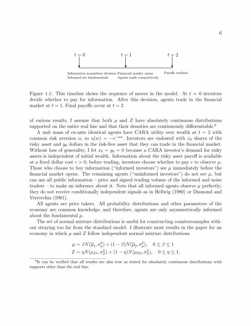
Figure 1.1: This timeline shows the sequence of moves in the model. At t = 0 investorsdecide whether to pay for information. After this decision, agents trade in the financialmarket at t = 1. Final payoffs occur at t = 2.

of various results, I assume that both µ and Z have absolutely continuous distributionssupported on the entire real line and that their densities are continuously differentiable.6

A unit mass of ex-ante identical agents have CARA utility over wealth at t = 2 withcommon risk aversion α, so u(w) = −e−αw. Investors are endowed with x0 shares of therisky asset and y0 dollars in the risk-free asset that they can trade in the financial market.Without loss of generality, I let x0 = y0 = 0 because a CARA investor’s demand for riskyassets is independent of initial wealth. Information about the risky asset payoff is availableat a fixed dollar cost c > 0; before trading, investors choose whether to pay c to observe µ.Those who choose to buy information (“informed investors”) see µ immediately before thefinancial market opens. The remaining agents (“uninformed investors”) do not see µ, butcan use all public information – price and signed trading volume of the informed and noisetraders – to make an inference about it. Note that all informed agents observe µ perfectly;they do not receive conditionally independent signals as in Hellwig (1980) or Diamond andVerrecchia (1981).

All agents are price takers. All probability distributions and other parameters of theeconomy are common knowledge, and therefore, agents are only asymmetrically informedabout the fundamental µ.

The set of normal mixture distributions is useful for constructing counterexamples with-out straying too far from the standard model. I illustrate most results in the paper for aneconomy in which µ and Z follow independent normal mixture distributions

µ ∼ βN(µ1, σ2µ) + (1− β)N(µ2, σ

2µ), 0 ≤ β ≤ 1

Z ∼ ηN(µZ1, σ2Z) + (1− η)N(µZ2, σ

2Z), 0 ≤ η ≤ 1.

6It can be verified that all results are also true as stated for absolutely continuous distributions withsupports other than the real line.

7

1.2.1 Equilibrium

Let Pλ denote the equilibrium risky-asset price when the fraction of informed agents is λ.Let XI(µ, Pλ) denote the number of shares demanded by an informed agent as a functionof fundamental µ and price. Since the informed types know the realized value of µ, theirdemand takes the standard mean-variance form XI(µ, Pλ) = µ−Pλ

ασ2ε.

When the uninformed agents choose their demands, they have access to the price andthe signed volume (order flow) of the informed and noise traders.7 Noise traders supply Zshares, so the signed trading volume of the informed and noise traders is λXI(µ, Pλ) − Z.However, it will turn out to be more convenient to work with the informationally-equivalentadjusted volume, defined as follows.

Definition 1.2.1 (Adjusted volume). The adjusted volume µλ of the informed and noisetraders is

µλ := µ− ασ2ε

λZ.

The adjusted volume µλ is a transformation of the price and signed volume.8 To compute

adjusted volume, the uninformed need only to multiply the signed volume by the constant ασ2ε

λ

and then add the price Pλ. Their information set provides sufficient information to performthese calculations.

Let XU(µλ, Pλ) denote the demand of the uninformed as a function of the adjusted volumeand price. The definition of equilibrium in the financial market is standard.

Definition 1.2.2 (Financial market equilibrium). A rational expectations equilibrium inthe financial market is a (measurable) price function Pλ(µ, Z) mapping R2 7→ R, and de-mand functions for the informed agents XI and uninformed agents XU such that all agentsmaximize expected utility, conditional on their information sets

XI(µ, Pλ) ∈ arg maxx∈R

E [u(x(D − Pλ))|µ, Pλ]

XU(µλ, Pλ) ∈ arg maxx∈R

E [u(x(D − Pλ))|µλ, Pλ] ,

and markets clear for each possible (µ, Z) pair

λXI(µ, Pλ) + (1− λ)XU(µλ, Pλ) = Z.

7In the standard model signed volume provides redundant information; traders need only to observe price.In more general settings, signed volume may refine the information contained in price. In some results inthis section I distinguish between the case in which investors condition only on price and the case in whichthey also observe signed volume.

8A similar variable, labeled wλ, appears in the original Grossman and Stiglitz (1980) paper. I choose theµλ notation to emphasize that this variable will be interpreted as a signal about µ.

8

All statements in the paper about equality of random variables, such as the marketclearing condition in Definition 1.2.2, should be understood to mean that the equality holdsalmost surely under the joint distribution of (µ, Z, ε), and all statements about equality offunctions on Rn should be understood to mean that the equality holds almost everywherewith respect to Lebesgue measure on Rn. To avoid unnecessary technical clutter, I refrainfrom making this explicit in the results and exposition below.

If the random variables in the model were jointly normally distributed, I would now solvefor the equilibrium by conjecturing a price function that is linear in the fundamental µ andsupply Z, solving the uninformed investors’ inference and portfolio problem given the pricefunction, and then substituting the resulting demand into the market clearing condition.This would produce a system of three equations with three unknowns (the coefficients in theprice function). In this simple setting, the coefficient equations would have explicit closed-form solutions. With a non-normal joint distribution, this solution technique is not possiblesince the functional form of the price is not clear a priori. Indeed, the best outcome one canhope for is to characterize the price as an implicit function of µ and Z.

The following result characterizes the equilibrium asset price, assuming that it exists.(Proofs of all results are relegated to Section 1.6.2.) The key step is to first solve a generalversion of the uninformed investors’ optimization problem, assuming that they conjecture anarbitrary price function. Since, in equilibrium, the quantity demanded by the uninformedmust be equal to the residual supply of the noise traders after subtracting the informeddemand, substituting in from the market clearing condition pins down a risky-asset pricethat both clears the market and is consistent with the uninformed investors’ beliefs.

Proposition 1.2.1. If there exists an equilibrium price function, Pλ(µ, Z), then it is implic-itly defined as

∫R

((1− λ)y + λ

(µ− ασ2

ελ Z

)− Pλ

)e

λ1−λ

µ−ασ2ελ

Z−Pλσ2ε

yfZ

(λασ2

ε

(y −

(µ− ασ2

ελ Z

)))fµ(y) dy = 0.

(1.1)

Looking at the relation in eq. (1.1), it is apparent that price depends on µ and Z only

through the adjusted volume µλ = µ − ασ2ε

λZ, which leads immediately to the following

Corollary.

Corollary 1.2.2. If it exists, the equilibrium price Pλ in Proposition 1.2.1 can be charac-terized as a function of the adjusted volume µλ only,∫

R((1− λ)y + λµλ − Pλ) e

λ1−λ

µλ−Pλσ2ε

yfµ|µλ(y|µλ) dy = 0. (1.2)

From this point forward, I treat Pλ as a univariate function mapping realizations m ofadjusted volume µλ into an equilibrium price, as in Corollary 1.2.2. There is no loss, however,

9

in continuing to think of price as a function of the fundamental µ and supply Z that dependson them only through the linear combination µλ.

To better understand the meaning of the integral in eq. (1.2), note that one can also writeit as an integral over realizations of the payoff D = µ + ε rather than just the fundamentalµ. Rearranging the resulting expression and writing out the utility function in general terms,u(·), gives

Pλ =

∫R yu

′(− λ

1−λµλ−Pλασ2

ε(y − Pλ)

)fD|µλ(y|µλ) dy∫

R u′(− λ


ε(y − Pλ)

)fD|µλ(y|µλ) dy

.

This looks like the standard representative agent pricing formula except that the “endow-ment” of the agent, − λ


ε, is endogenous. Accordingly, one can interpret eq. (1.2) as

a representative agent pricing formula in which the representative uninformed agent’s equi-librium risky asset holding is the residual supply of the noise traders, net of the demand ofthe informed investors.

It is clear from eq. (1.2) that the price is a nonlinear function of the fundamental µ andsupply Z. However, because the residual uncertainty ε is normally distributed and utilityfunctions are exponential, the information conveyed by price is still a linear combination µλof the quantities µ and Z, as in the standard model. While this fact simplifies the analysisof the information content of prices, it is not vital for my results. Indeed, allowing for amore general distribution for ε would provide one more degree of freedom with which toconstruct counterexamples to standard results. Similarly, one could criticize the restrictionto exponential utility, which precludes income effects. However, this also makes constructionof counterexamples more difficult. Indeed, including nontrivial income effects would tend tostrengthen most of the results in the paper.

Proposition 1.2.1 assumes existence of an equilibrium in the financial market. The fol-lowing proposition gives a sufficient condition for existence.

Proposition 1.2.3. If for each fixed m ∈ R the conditional moment generating function ofµ given µλ = m exists in an open neighborhood around zero, then there exists an equilibriumprice function Pλ.

The restriction that µ has a moment generating function (mgf) is needed so that expectedutility exists (expected utility for a CARA investor is essentially a moment-generating func-tion) and the integral in eq. (1.2) converges. As long as the integral is finite, then the existenceof an equilibrium price that satisfies eq. (1.2) follows from the intermediate value theorem.Unfortunately, the restriction on the distribution of fundamentals in the proposition rulesout fat-tailed distributions, along with lognormal distributions.9

9Difficulty incorporating fat-tailed distributions into an otherwise-standard economy with expected-utility-maximizing investors is not specific to my model. Geweke (2001) points out the same problem ina setting with a CRRA representative investor when log returns follow a t-distribution.

10

So far, I have said nothing of uniqueness. In principle, for some realizations of µλ therecould be multiple values of Pλ that satisfy (1.2).10 Fortunately, that is not the case, andthe equilibrium price defined by eq. (1.2) is unique, at least within the class of continuouslydifferentiable functions.

Proposition 1.2.4. The function defined by (1.2) is the unique continuously differentiableprice function.

In some sense, the uniqueness result should not be surprising. In models in which agentsdo not learn from prices, multiplicity can arise if wealth effects are sufficiently strong toprevent aggregate demand from sloping downward at all prices. Exponential utility rulesout wealth effects, and as indicated in Proposition 1.4.2, one can reduce the model to one inwhich the uninformed do not condition on price but instead observe only adjusted volume µλ.Hence, the presence of only substitution effects means that for given µλ, aggregate demandis downward sloping, and therefore the equilibrium price is unique.

A Corollary of Proposition 1.2.4 is that the linear equilibrium in the standard model isin fact (essentially) unique, not merely unique among linear equilibria. To my knowledge,this was still an open question.

Corollary 1.2.5. When µ and Z are independently normally distributed, the linear pricefunction given in Grossman and Stiglitz (1980) is the unique continuously differentiable pricefunction.

This completes the analysis of equilibrium in the financial market. Next, I addressequilibrium in the information market.

Information market equilibrium

While it is not the focus of this paper, for completeness I now define equilibrium in theinformation market. Let CE(λ) denote the ex-ante certainty-equivalent gain CE (gross ofcost c) from becoming informed as a function of the fraction λ of informed agents

CE(λ) := − 1

αlogE[e−αXI(µ,Pλ)(D−Pλ)]︸︷︷︸

Informed certainty-equivalent wealth

− − 1

αlogE[e−αXU (µλ,Pλ)(D−Pλ)]︸︷︷︸

Uninformed certainty-equivalent wealth

. (1.3)

I use a standard definition of equilibrium in the information market, identical to that usedby Grossman and Stiglitz (1980). To add realism, one could more explicitly model aninformation production sector as in, for example, Admati and Pfleiderer (1986) or Veldkamp(2006b). However, for simplicity and comparability with earlier work I choose the most basicpossible setup.

10Technically speaking, eq. (1.2) defines a correspondence from which an equilibrium price must be selected.In principle, this correspondence might not be single-valued.

11

Definition 1.2.3 (Information market equilibrium). An equilibrium in the information mar-ket is a fraction λ∗ ∈ [0, 1] such that,

• λ∗ = 0 and CE(0) ≤ c, or

• λ∗ ∈ (0, 1) and CE(λ∗) = c, or

• λ∗ = 1 and CE(1) ≥ c.

Definition 1.2.3 says that an equilibrium in the information market falls into one of threepossible cases. Either (1) no one buys information because the cost of doing so exceeds thebenefit, even if no one else buys any, or (2) there is an interior value for λ∗ such that at themargin the gain from acquiring information is exactly equal to the cost of doing so, or (3)everyone buys information because it is sufficiently cheap that the benefit always outweighsthe cost, regardless of how many others buy information.

Existence and uniqueness of equilibrium in the information market is a more delicatematter than existence and uniqueness in the financial market. Since information marketequilibria depend on the value of acquiring information, I postpone further discussion untilI take up the value of information in Section 1.4.3.

In noisy REE models, investors use available signals to make an inference about funda-mentals. In my model, from the standpoint of the uninformed investors the signal is theadjusted volume µλ, and the variable that they are trying to learn about is the fundamentalµ. The main results presented later on the value of technical analysis, the shape of uninformedinvestor demand curves, and the value of acquiring information depend on how uninformedinvestors react to the information contained in price. It turns out that a monotone likelihoodratio property (MLRP) for signals is the appropriate concept for characterizing reaction toinformation.

1.3 Discussion of the monotone likelihood ratio prop-

erty

While the MLRP is familiar to most readers, in this section I will briefly restate the definition,discuss the implications for investor behavior, and tie the MLRP to a restriction on thedistribution of noise in the economy.11 Briefly, in my model the MLRP guarantees thatuninformed investors’ demand reacts in the “correct” direction to changes in adjusted volumeµλ, and it requires that the distribution of noise satisfy a particularly stringent unimodalitycondition. In more general terms, requiring the MLRP for endogenous signals in a noisy REEmodel guarantees that “good news” for one agent is also “good news” for other agents wholearn about her information by looking at the price (or other market data), and it requiresthat signals be affiliated with fundamentals.

11Milgrom (1981) is a standard reference for the MLRP.

12

I begin by stating the definition of the monotone likelihood ratio property.

Definition 1.3.1 (Monotone likelihood ratio property). Consider any two random variablesX and Y. The family of conditional densities {fX|Y (·|y)}y∈Support(Y ) satisfies the monotonelikelihood ratio property (MLRP) if for all x′ > x and y′ > y, the following inequality holds

fX|Y (x′|y′)fX|Y (x|y) ≥ fX|Y (x′|y)fX|Y (x|y′). (1.4)

If the inequality in eq. (1.4) is strict at every set of points, the family is said to satisfy thestrict MLRP.

It is helpful to think of the random variable X as a signal providing information about Y.If the conditional densities of the signal X have the MLRP, then increases in X shift “up”the posterior distribution of Y in the monotone likelihood ratio (MLR) stochastic order

(i.e., given x′ > x, the likelihood ratio of the posteriorsfY |X(y|x′)fY |X(y|x)

is increasing in y). The

MLR ordering is a strengthening of the well-known first-order stochastic dominance (FOSD)ordering.12 In fact, Proposition 2 of Milgrom (1981) shows that a family of conditionaldensities {fX|Y } has the MLRP if and only if higher values of the signal X improve theposterior distribution of Y in the FOSD sense under any prior for Y. With only two randomvariables, the MLRP is equivalent to their being affiliated. See Milgrom and Weber (1982)for a detailed discussion of affiliation.

In my model, if the conditional densities of adjusted volume fµλ|µ have the MLRP thenhigher values of adjusted volume µλ imply MLR improvements in the risky asset payoff.Recalling that µλ can be written as a linear combination of the fundamental and supply,

µλ = µ− ασ2ε

λZ, this implies that for a given realization of supply Z, both the informed and

uninformed experience an MLR improvement in response to an increase in the fundamentalµ; their beliefs react in the same direction to fundamentals. I provide more detail for thisresult below when discussing implications for investor demand.

Since adjusted volume µλ is not one of the primitives of the model, it is helpful to have acondition on the underlying random variables that determines whether fµλ|µ has the MLRP.The following Lemma provides an equivalent condition on the distribution fZ of the assetsupply.

Lemma 1.3.1. The conditional densities fµλ|µ satisfy the (strict) MLRP if and only if log fZis (strictly) concave.13

An alternative, but equivalent, characterization of Lemma 1.3.1 is that fµλ|µ satisfiesthe MLRP if and only if the distribution of asset supply is strongly unimodal.14 Requiring

12Eeckhoudt and Gollier (1995) provide a proof, as well as an example that satisfies FOSD but not MLR.See also Chapter 1.C of Shaked and Shanthikumar (2007) for further discussion of the MLR order.

13An (1998) and Bagnoli and Bergstrom (2005) discuss logconcavity and related properties.14A density on the real line is unimodal if for all K > 0, the set {x ∈ R|f(x) ≥ K} is convex. A density

is strongly unimodal if its convolution with any other unimodal distribution is unimodal. If a distribution isstrongly unimodal then it is unimodal, but the converse is not true.

13

a logconcave distribution rules out fat-tailed noise distributions (Karlin, 1968, Proposition7.1.4) as well as both multimodal distributions and unimodal ones that are not stronglyunimodal. Counterexamples to logconcavity (and thus the MLRP) need not be pathological.The normal mixture examples used in this paper to break the MLRP can be thought ofas a world with higher-order uncertainty: noise trade is typically drawn from a normaldistribution with, say, a mean of one, but with some small probability it is drawn froma distribution with a much higher mean, in which case noise traders flood with marketwith a large number of shares. Similarly, neither lognormal nor binomial distributions arelogconcave. Even if one restricts attention to unimodal distributions with “nice” intuitiveproperties, logconcavity does not necessarily follow. Given a (bounded) distribution for theunderlying state µ, Chambers and Healy (2009) exhibit a unimodal, symmetric, mean-zeroerror term (the analogue to supply in my model) and a range of signals over which posteriorsdeteriorate in the sense of FOSD.

In Figure 1.2(a), I plot the posterior beliefs about µ for increasing realizations of adjustedvolume µλ when distributions are normal and therefore the MLRP is satisfied. The solid linecorresponds to the lowest realization of µλ, followed by the dashed line, and then the dottedline. Notice that higher signal realizations correspond unambiguously to “higher” posteriordistributions. On the other hand, if the supply distribution Z is, say, a bimodal mixtureof normals, then signals do not have the MLRP. Figure 1.2(c) plots the analogous poste-rior beliefs in such an economy for increasing realizations of µλ. In this case, the posteriordistribution corresponding to the highest signal (dotted line) is actually “lower” than theother two, which illustrates the fact that once signals fail to have the MLRP, the uninformedposterior beliefs do not necessarily move in the “correct” direction when µ changes.

Moving beyond probability assessments, it should be apparent that the way in whichbeliefs react to signals has implications for the way in which agents trade in response tosignals. An upward shift in an asset’s payoff distribution (for instance, an FOSD improve-ment) has both substitution and income effects in general (though income effects are absentwith exponential utility). However, the signs and magnitudes of the effects vary, so theoverall effect on demand is ambiguous without adding further restrictions on either utilityfunctions or random variables.15 To obtain clear comparative statics, one must restrict theclass of upward shifts considered. As first noted by Landsberger and Meilijson (1990), MLRimprovements are sufficient for all nonsatiated investors to demand a greater quantity ofthe risky asset in a single-risky-asset portfolio problem. Athey (2002, Lemma 5) proves thestronger result that MLR shifts are in fact necessary and sufficient for any nonsatiated in-vestor to rebalance her portfolio in the expected direction regardless of the price of the risky

15It is a common misconception that FOSD improvements in a risky asset are sufficient for increaseddemand. As first pointed out by Fishburn and Porter (1976), this is not true without further restrictions onthe utility function. Note that despite the lack of wealth effects, FOSD is not sufficient even for exponentialutility. Fishburn and Porter (1976), Kira and Ziemba (1980), Cheng, Magill, and Shafer (1987), and Hadarand Seo (1990) provide conditions on utility functions that guarantee the “expected” comparative staticsresults for stochastic dominance shifts in various formulations of the portfolio problem.

14

7 8 9 10Μ

0.2

0.4

0.6

0.8

1.0

fΜ Μ

`

(a) Beliefs (with MLRP)

15 20XU

1

2

3

4

5

P

(b) Uninformed demand (with MLRP)

7 8 9 10Μ

0.2

0.4

0.6

0.8

fΜ Μ

`

(c) Beliefs (without MLRP)

-6 -4 -2 2 4 6XU

6

7

8

9

10

11

P

(d) Uninformed demand (without MLRP)

Figure 1.2: Plots of uninformed demand curves for increasing realizations of µλ, along withthe associated posterior beliefs. The lowest realization of µλ is represented by the solidline, next highest by the dashed line, and highest by the dotted line. For comparability, inthe plots of beliefs the prior fµ is included as the light gray line. In panels (a) and (b),η = 1, µZ = 1, while in panels (c) and (d), η = 8/10, µZ1 = 1, µZ2 = 4. Other parameters arethe same: β = 1, µ = 8, σµ = 1/2, σZ = 1/2, σε = 1/2, α = 1.

15

asset. In other words, requiring the MLRP is equivalent not only to requiring that beliefs ofboth types respond in the same direction to changes in µ, but more importantly that theirdemands move in the same direction, regardless of the price that prevails in the market.

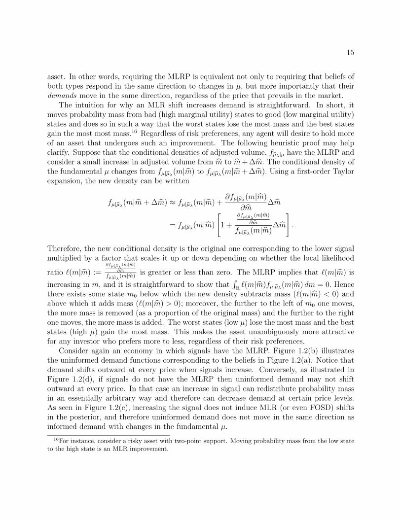
The intuition for why an MLR shift increases demand is straightforward. In short, itmoves probability mass from bad (high marginal utility) states to good (low marginal utility)states and does so in such a way that the worst states lose the most mass and the best statesgain the most most mass.16 Regardless of risk preferences, any agent will desire to hold moreof an asset that undergoes such an improvement. The following heuristic proof may helpclarify. Suppose that the conditional densities of adjusted volume, fµλ|µ have the MLRP andconsider a small increase in adjusted volume from m to m+ ∆m. The conditional density ofthe fundamental µ changes from fµ|µλ(m|m) to fµ|µλ(m|m+ ∆m). Using a first-order Taylorexpansion, the new density can be written

fµ|µλ(m|m+ ∆m) ≈ fµ|µλ(m|m) +∂fµ|µλ(m|m)

∂m∆m

= fµ|µλ(m|m)

[1 +

∂fµ|µλ (m|m)

∂m

fµ|µλ(m|m)∆m

].

Therefore, the new conditional density is the original one corresponding to the lower signalmultiplied by a factor that scales it up or down depending on whether the local likelihood

ratio `(m|m) :=∂fµ|µλ

(m|m)

∂m

fµ|µλ (m|m)is greater or less than zero. The MLRP implies that `(m|m) is

increasing in m, and it is straightforward to show that∫R `(m|m)fµ|µλ(m|m) dm = 0. Hence

there exists some state m0 below which the new density subtracts mass (`(m|m) < 0) andabove which it adds mass (`(m|m) > 0); moreover, the further to the left of m0 one moves,the more mass is removed (as a proportion of the original mass) and the further to the rightone moves, the more mass is added. The worst states (low µ) lose the most mass and the beststates (high µ) gain the most mass. This makes the asset unambiguously more attractivefor any investor who prefers more to less, regardless of their risk preferences.

Consider again an economy in which signals have the MLRP. Figure 1.2(b) illustratesthe uninformed demand functions corresponding to the beliefs in Figure 1.2(a). Notice thatdemand shifts outward at every price when signals increase. Conversely, as illustrated inFigure 1.2(d), if signals do not have the MLRP then uninformed demand may not shiftoutward at every price. In that case an increase in signal can redistribute probability massin an essentially arbitrary way and therefore can decrease demand at certain price levels.As seen in Figure 1.2(c), increasing the signal does not induce MLR (or even FOSD) shiftsin the posterior, and therefore uninformed demand does not move in the same direction asinformed demand with changes in the fundamental µ.

16For instance, consider a risky asset with two-point support. Moving probability mass from the low stateto the high state is an MLR improvement.

16

Up to now, I have said nothing of market clearing, but have merely described how agentsreact to signals, holding all else fixed. However, it should be unsurprising to learn that sincethe MLRP guarantees that the uninformed react in the “correct” direction to signals, italso guarantees that the market-clearing price reacts in the correct direction. To understandwhy this is, it may be helpful to first think about a model where there are no uninformedtypes. Consider an economy populated by only informed investors and noise traders. Inthis case, price always reacts in the expected direction. If the fundamental µ increases then,since changes in µ represent MLR shifts under the informed information set, the informedinvestors demand a greater quantity of risky asset at every price; therefore, in order toclear the market the equilibrium price must increase with µ, holding supply Z constant.Conversely, an increase in supply Z means that the informed must accommodate a greaternumber of shares at any level of the fundamental µ, so price must decrease in Z for fixed µ.

Now consider the same thought experiment of making a small change to the fundamentalµ or supply Z but introduce uninformed investors who try to infer µ. If µ increases, thenthe informed demand curve still shifts outward at every price. The uninformed, on theother hand, do not observe µ, only a noisy signal in the form of the adjusted volume µλ.

17

Since the uninformed demand does not always shift outward with higher signals, it followsthat the aggregate demand will not necessarily shift outward either. As such, higher signals(corresponding, for instance, to higher realizations of µ) will not necessarily correspond tohigher prices. The only way to guarantee a monotone price function for any prior fµ is toimpose the MLRP for the signal distribution fµλ|µ so that uninformed demand, and henceaggregate demand, shifts in the same direction as the fundamental.

1.4 General results

1.4.1 Uninformed demand and the information content of prices

In rational expectations models, price affects uninformed investor demand in multiple ways.First, a change in price will cause uninformed investors to modify their demand due to astandard substitution effect. Secondly, since price conveys a signal about the fundamental,there is an information effect: if higher prices signal higher fundamentals, uninformed de-mand will increase with price. In the standard model, all prices are equally informative, andequilibrium demand curves for the uninformed slope down. In other words, the substitutioneffect of an increase in price dominates the information effect. However, this depends on thejoint distribution of fundamentals and price. In general, conditional moments of fundamen-tals will vary nontrivially with the price level. For certain regions of price, the informationeffect may dominate, leading to backward-bending demand. In such regions price responds

17Note that here I am simply endowing the uninformed with the signal µλ and considering how theirdemand changes; there is no explicit learning from price. Proposition 1.4.2 below implies that doing so doesnot change the results.

17

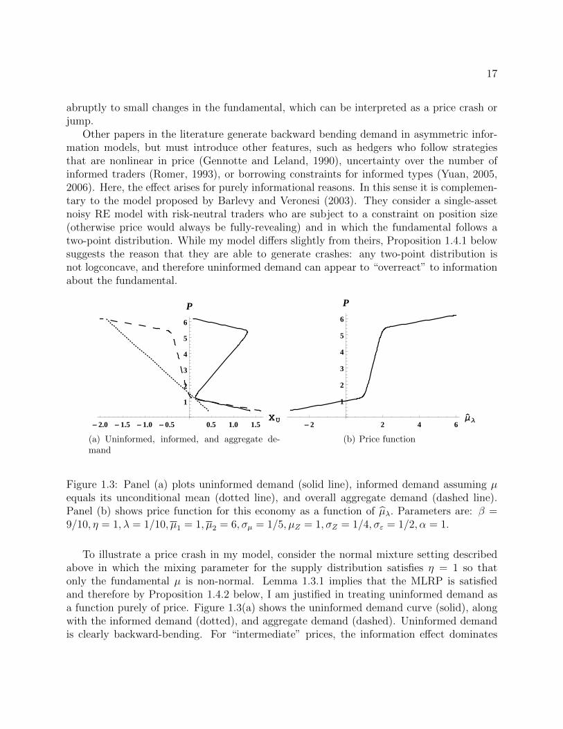
abruptly to small changes in the fundamental, which can be interpreted as a price crash orjump.

Other papers in the literature generate backward bending demand in asymmetric infor-mation models, but must introduce other features, such as hedgers who follow strategiesthat are nonlinear in price (Gennotte and Leland, 1990), uncertainty over the number ofinformed traders (Romer, 1993), or borrowing constraints for informed types (Yuan, 2005,2006). Here, the effect arises for purely informational reasons. In this sense it is complemen-tary to the model proposed by Barlevy and Veronesi (2003). They consider a single-assetnoisy RE model with risk-neutral traders who are subject to a constraint on position size(otherwise price would always be fully-revealing) and in which the fundamental follows atwo-point distribution. While my model differs slightly from theirs, Proposition 1.4.1 belowsuggests the reason that they are able to generate crashes: any two-point distribution isnot logconcave, and therefore uninformed demand can appear to “overreact” to informationabout the fundamental.

-2.0 -1.5 -1.0 -0.5 0.5 1.0 1.5XU

1

2

3

4

5

6

P

(a) Uninformed, informed, and aggregate de-mand

-2 2 4 6Μ`

Λ

1

2

3

4

5

6

P

(b) Price function

Figure 1.3: Panel (a) plots uninformed demand (solid line), informed demand assuming µequals its unconditional mean (dotted line), and overall aggregate demand (dashed line).Panel (b) shows price function for this economy as a function of µλ. Parameters are: β =9/10, η = 1, λ = 1/10, µ1 = 1, µ2 = 6, σµ = 1/5, µZ = 1, σZ = 1/4, σε = 1/2, α = 1.

To illustrate a price crash in my model, consider the normal mixture setting describedabove in which the mixing parameter for the supply distribution satisfies η = 1 so thatonly the fundamental µ is non-normal. Lemma 1.3.1 implies that the MLRP is satisfiedand therefore by Proposition 1.4.2 below, I am justified in treating uninformed demand asa function purely of price. Figure 1.3(a) shows the uninformed demand curve (solid), alongwith the informed demand (dotted), and aggregate demand (dashed). Uninformed demandis clearly backward-bending. For “intermediate” prices, the information effect dominates

18

the substitution effect, and demand rises with price. However, once price is sufficiently highor low, the uninformed are again relatively certain about the state of the world, and thedemand curve is downward-sloping. This fits with the intuition that an “extreme” price ismore informative than an intermediate price: when price is very high or low, small changeshave mostly substitution effects.

Backward-bending uninformed demand can lead to a price function that is particularlysteep over narrow regions of fundamentals. In Figure 1.3(b), I plot the price function for thesame economy as the demand functions in Figure 1.3(a). Notice that for values of adjustedvolume µλ near 1.75 small shocks can cause large changes in price. Such extreme pricereactions to small disturbances to fundamentals can be interpreted as crashes or jumps.

The example above is an illustration of the following result.

Proposition 1.4.1 (Backward-bending demand). Assume that the distribution of adjustedvolume given the fundamental fµλ|µ has the strict MLRP and that the price function isdifferentiable.18

• If there exists m < m′ such that for µλ ∈ [m, m′] the price function satisfies ∂Pλ∂m

> 1,then uninformed demand slopes up for prices in the interval [Pλ(m), Pλ(m

′)].

• If log fµ is concave, then ∂Pλ∂m≤ 1 and uninformed demand is everywhere downward-

sloping.

Recalling that the adjusted volume can be written µλ = µ − ασ2ε

λZ, one can interpret

Proposition 1.4.1 as a condition on how strongly price reacts to a change in the fundamentalµ. If there is a region of fundamentals in which prices “overreact” in the sense of movingmore than dollar-for-dollar with µ, then that coincides with the region in which uninformeddemand is backward-bending. This makes sense intuitively: A sufficiently strong informationeffect means that a change in price is self-reinforcing since the uninformed demand moves inthe same direction as the price. A sufficient condition for downward-sloping demand is thatthe distribution of the fundamental is logconcave. This essentially guarantees that smallchanges in µλ are not “too informative,” in the sense of moving the posterior expectation ofµ by more than the change in µλ itself.

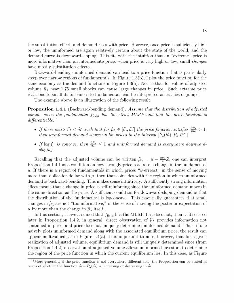
In this section, I have assumed that fµλ|µ has the MLRP. If it does not, then as discussedlater in Proposition 1.4.2, in general, direct observation of µλ provides information notcontained in price, and price does not uniquely determine uninformed demand. Thus, if onenaively plots uninformed demand along with the associated equilibrium price, the result canappear multivalued, as in Figure 1.4(a). It is important to note, however, that for a givenrealization of adjusted volume, equilibrium demand is still uniquely determined since (fromProposition 1.4.2) observation of adjusted volume allows uninformed investors to determinethe region of the price function in which the current equilibrium lies. In this case, as Figure

18More generally, if the price function is not everywhere differentiable, the Proposition can be stated interms of whether the function m− Pλ(m) is increasing or decreasing in m.

19

1.4(b) illustrates (and as discussed in detail in Section 1.4.2), changes in fundamentals cancause price to be decreasing in adjusted volume over certain regions.

-2.0 -1.5 -1.0 -0.5 0.5 1.0 1.5Demand

1.5

2.0

P

(a) Uninformed, informed, and aggregate demand

-2 2 4 6Μ`

Λ

1.5

2.0

P

(b) Price function

Figure 1.4: Panel (a) plots uninformed demand (solid line), informed demand assuming µequals its unconditional mean (dotted line), and overall aggregate demand (dashed line).Panel (b) shows price function for this economy as a function of µλ. Parameters are: β =1, η = 8/10, λ = 1/10, µ = 5/4, σµ = 1/2, µZ1 = −1, µZ2 = 2, σZ = 1/2, σε = 1/2, α = 1

Unlike other models in the literature, in my setting crashes and jumps arise withoutadding nonlinear hedgers, portfolio constraints, or additional uncertainty. All that is requiredis that in some regions, the uninformed learn at a particularly fast rate as price changes.This suggests that crashes may arise naturally for purely informational reasons, as long asthere is asymmetric information in the economy.

1.4.2 The value of observing signed volume

In the standard model the asset price provides all possible information that the uninformedcan glean from public sources, and observing (signed) volume, aggregate order flow, or anypublic quantity other than the current price provides no additional information.19 Blume,Easley, and O’Hara (1994) and Schneider (2009) study more complex models in which ob-serving trading volume is useful for investors. Blume, Easley, and O’Hara (1994) considera dynamic model in which the precision of some traders’ signals is random. However, theyassume that investors are not able to condition on current price, only past prices. Combinedwith observations of the current price, observing volume provides a way to learn about theunknown signal precisions. Schneider (2009) studies an otherwise-standard static model butassumes that the correlation between investors’ signals is random; trading volume allows

19This is not necessarily true in models in which traders have diverse information such as Diamond andVerrecchia (1981). In those models, if traders can condition on volume and the sign of their own trade, thena fully-revealing equilibrium exists. See Blume, Easley, and O’Hara (1994) for a heuristic proof.

20

them to determine whether they are in the high correlation or low correlation state. Twoother related papers in the technical analysis literature are Brown and Jennings (1989) andGrundy and McNichols (1989), both of which study three-date dynamic models in whichpast prices are informative when used in conjunction with the current price.

While these other studies require introduction of either uncertainty about some quantityother than fundamentals or additional rounds of trade, the following proposition shows thata similar result can hold even when investors need only to learn about the asset payoff, andthere is no uncertainty over information quality or diversity.

Proposition 1.4.2 (Information content of adjusted volume).

(i) If the conditional distribution of adjusted volume given the fundamental, fµλ|µ, has thestrict MLRP, then the price function is strictly increasing in adjusted volume µλ andobserving Pλ provides the same information to the uninformed as observing µλ.

(ii) If fµλ|µ does not have the strict MLRP, then observing µλ provides more informationthan Pλ in the following sense: depending on the distribution of the fundamental, µ,there may exist realizations m′ 6= m of µλ for which Pλ(m

′) = Pλ(m).

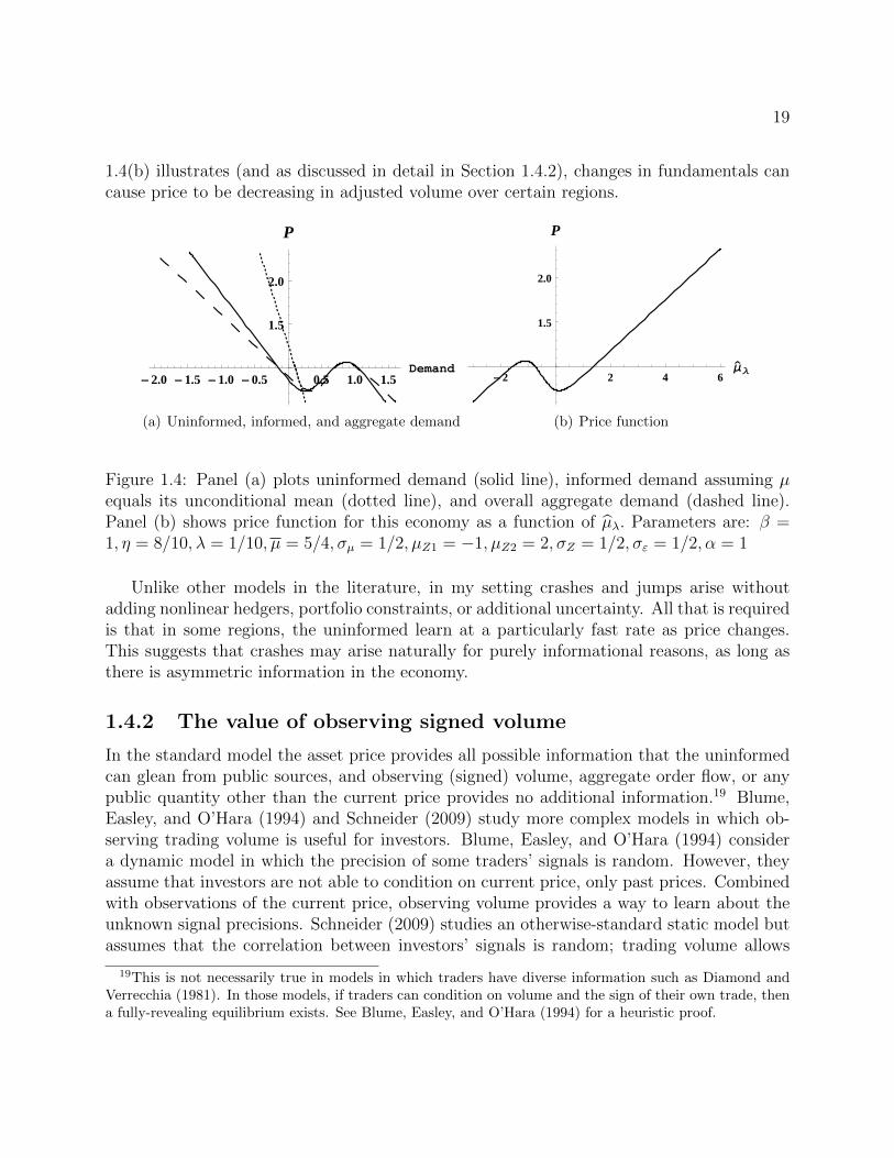
The first result in Proposition 1.4.2 is equivalent to the fact that with the MLRP, theprice function is strictly increasing in adjusted volume µλ. In that case, each realization ofPλ is associated with a unique value of µλ, and price provides exactly the same informationas direct observation of adjusted volume µλ. An increase in fundamental µ MLR-improvesthe investment opportunity set for both types which increases the aggregate demand andtherefore increases the price. Figure 1.5(a) illustrates a monotone price function for thenormal mixture setting introduced above in which the mixing parameter for the fundamentalsatisfies β = 1 so that only supply is non-normal.

The second result in Proposition 1.4.2 says that without the MLRP, there may existprices that are consistent with two or more distinct realizations of adjusted volume µλ.

20

If the distribution of µλ does not have the MLRP then one cannot guarantee that bothinformed and uninformed types react in the same direction (as in Figure 1.2(d) above) andthus that the price moves in the same direction. Nonmonotonicity of the price function mayseem surprising at first; however, in light of the discussion in Section 1.3 it is in some senseobvious. Informed and uninformed demand may shift in opposite directions in response toincreases in the fundamental µ, and over certain regions the uninformed reaction may besufficiently strong to decrease the price. In those situations, the price is no longer a sufficientstatistic for learning about µ, and the adjusted volume allows the uninformed to distinguishbetween the various regions of the price function. This is illustrated in Figure 1.5(b) in whichthe price function is non-monotone, and there are some realizations of price that correspondto three possible values of µλ.

20Note that if the uninformed were able to observe only the price, it follows from Lemma 1.6.3 that aµλ-measurable equilibrium would fail to exist in these situations.

21

Nonmonotonic price functions also arise in asymmetric information models with feed-back effects due to endogenous firm investment decisions (Dow and Rahi, 2003) or regula-tory intervention (Bond, Goldstein, and Prescott, 2010). For instance, in Bond, Goldstein,and Prescott (2010), a given price may correspond to both a low-fundamental, positive-intervention state as well as a high-fundamental, no-intervention state. In my model, cashflows are exogenous, but there is a similar explanation with respect to the fundamental andnoisy supply. Recall that in the normal mixture setting, one can think of the noisy supplyrealization as coming from a two-step procedure: first choose the ‘high’ or ‘low’ supply dis-tribution, and then draw the supply from that distribution. In such a situation, the sameprice can arise in three distinct states. As the adjusted volume moves from ‘high’ values to‘low’ values, the uninformed become become relatively confident that the low realization canbe attributed to a draw from the ‘high mean’ supply distribution. Hence, they are willing toaccommodate more of the asset than if they believed that the low realization was due to alow value for the fundamental µ. Hence, depending on the distribution of supply, a relativelylow realization of µλ may actually be good news.

-5 5Μ`

Λ

4

5

6

7

8

PΛ

(a) Monotone price function

-5 5Μ`

Λ

4

5

6

7

8

PΛ

(b) Non-monotone price function

Figure 1.5: Plots of equilibrium price functions. In panel (a), µZ2 = 3, σZ = 1, while inpanel (b), µZ2 = 5, σZ = 1/2. Other parameters are the same: β = 1, η = 9/10, µ = 8, σµ =1, µZ1 = 0, σε = 1/2, α = 1, λ = 1/10.

As the empirical analogue of adjusted volume is net order flow, this provides a potentialexplanation of the value of observing order flow: it contains information about aggregatedemand that is not contained in price alone. This is reminiscent of the point made byGallmeyer, Hollifield, and Seppi (2005) that the trading process itself can reveal informationabout the trading motive of one’s counterparties. The results presented here are complemen-tary in that their model focuses on learning effects with regard to unknown preferences andthe consequences for future resale prices, while my model focuses on learning effects withregard to cash flows in a static model.

22

The result that adjusted volume conveys incremental information is similar in spirit tothose of Blume, Easley, and O’Hara (1994) and Schneider (2009). In all cases, observationof a non-price statistic allows uninformed investors to more effectively learn from prices bymaking a previously non-invertible price function invertible.21 However, my result makesclear that it is not necessary to add additional uncertainty to the model to achieve this.Rather, what is required is to change the distribution of uncertainty in the economy in sucha way that the price function is no longer invertible. Whether one achieves this by, say,making signal quality random or simply changing the underlying probability distributions isimmaterial. What is key is that the change makes the price function nonmonotonic in thefundamental.

1.4.3 The value of acquiring information

In the standard model as the number of informed investors increases, price becomes moreinformative, and the uninformed are better able to free-ride on the informed types’ informa-tion. It follows that the value of observing the fundamental µ decreases with the numberof informed. In other words, information acquisition is a strategic substitute: as more in-vestors learn about µ, the incentive for others to do the same decreases. It has been an openquestion whether the opposite case (strategic complementarity in information acquisition) isalso possible in an otherwise-standard noisy RE model.

In these models, an increase in the number of informed investors has two competingeffects. It typically drives the asset price closer to the fundamental in each state (priceeffect), but it also changes the equilibrium allocations (share effect). The price effect tendsto reduce the total surplus that both types enjoy at the expense of the noise traders, and itreduces the share of that surplus taken by the informed investors. On the other hand, theshare effect requires that in equilibrium the remaining uninformed hold less advantageouspositions in the asset in order to accommodate the increased number of informed investors.In the standard model with normal distributions, the price effect is sufficiently strong tooffset the share effect. Price is responsive to information, which causes the price effect todominate the share effect and make information acquisition a strategic substitute.

In my model, I can characterize the price and share effects of a change in the fraction ofinformed, λ, directly.

Lemma 1.4.3 (Utility gain). Assume that the price function is differentiable with respectto m and λ. The derivative of the utility gain function CE with respect to the number of

21I do not mean invertible in the sense of fully-revealing. Here, invertible means that the price is monotonicin some (possibly noisy) aggregate of the information of all traders.

23

informed λ can be written as the sum of a price effect and a share effect

CE′(λ) = −∫∫

R2

(XI(m,Pλ(m))eI −XU (m, Pλ(m))eU

) [∂Pλ∂m

m−mλ + ∂Pλ

∂λ

]fµλ|µfµ dmdm︸︷︷︸

Price effect

−∫∫

R2

(m− Pλ(m)− ασ2

εXU (m, Pλ(m))) [

∂XU∂m + ∂XU

∂p∂Pλ∂m

]m−mλ eUfµλ|µfµ dmdm︸︷︷︸

Share effect

,

(1.5)

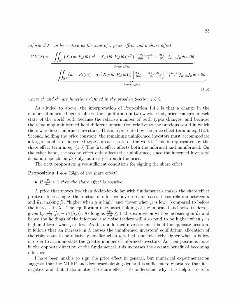
where eI and eU are functions defined in the proof in Section 1.6.2.

As alluded to above, the interpretation of Proposition 1.4.3 is that a change in thenumber of informed agents affects the equilibrium in two ways. First, price changes in eachstate of the world both because the relative number of both types changes, and becausethe remaining uninformed hold different information relative to the previous world in whichthere were fewer informed investors. This is represented by the price effect term in eq. (1.5).Second, holding the price constant, the remaining uninformed investors must accommodatea larger number of informed types in each state of the world. This is represented by theshare effect term in eq. (1.5) The first effect affects both the informed and uninformed. Onthe other hand, the second effect only affects the uninformed, since the informed investors’demand depends on µλ only indirectly through the price.

The next proposition gives sufficient conditions for signing the share effect.

Proposition 1.4.4 (Sign of the share effect).

• If ∂Pλ∂m≤ 1 then the share effect is positive.

A price that moves less than dollar-for-dollar with fundamentals makes the share effectpositive. Increasing λ, the fraction of informed investors, increases the correlation between µand µλ, making µλ “higher when µ is high” and “lower when µ is low” (compared to beforethe increase in λ). The equilibrium risky asset holding of the informed and noise traders isgiven by λ

ασ2ε

(µλ − Pλ(µλ)) . As long as ∂Pλ∂m≤ 1, this expression will be increasing in µλ and

hence the holdings of the informed and noise traders will also tend to be higher when µ ishigh and lower when µ is low. As the uninformed investors must hold the opposite position,it follows that an increase in λ causes the uninformed investors’ equilibrium allocation ofthe risky asset to be relatively smaller when µ is high and relatively higher when µ is lowin order to accommodate the greater number of informed investors. As their positions movein the opposite direction of the fundamental, this increases the ex-ante benefit of becominginformed.

I have been unable to sign the price effect in general, but numerical experimentationsuggests that the MLRP and downward-sloping demand is sufficient to guarantee that it isnegative and that it dominates the share effect. To understand why, it is helpful to refer

24

back to the discussion in Section 1.3. As explained there, with the MLRP, the uninformedinvestors’ demand reacts in the same direction as the informed to changes in the fundamentalµ. An increase in the number of informed λ makes the signal µλ more highly correlated withthe fundamental µ, and therefore makes uninformed demand more highly correlated withinformed demand. This drives the price closer to the fundamental (on average), reducingthe profit that the informed investors make from their information.

More precisely, it is straightforward to show that under the MLRP assumption, increasesin the fraction informed, λ, improve the accuracy (sometimes also called effectiveness) of thesignal µλ. Accuracy was introduced by Lehmann (1988) in the context of statistical decisiontheory as a generalization of Blackwell (1951, 1953) sufficiency, which is another common cri-teria for comparing signals. Persico (1996, 2000) introduced the use of accuracy in economiccontexts. Blackwell sufficiency was the definition of informativeness used by Grossman andStiglitz (1980). Unfortunately, many signals cannot be compared using Blackwell sufficiency.Accuracy allows the comparison of many more signals, as discussed by Lehmann (1988). Italso nests Blackwell sufficiency; if one signal is sufficient for another, then it is also moreaccurate.

The overall sign of the utility gain expression depends on the sign and strength of the twoeffects discussed above. As noted above, I have been unable to determine general conditionsunder which it is either increasing or decreasing. I present here some simple numerical exam-ples to illustrate situations in which, contrary to the standard result, information acquisitionis a strategic complement.

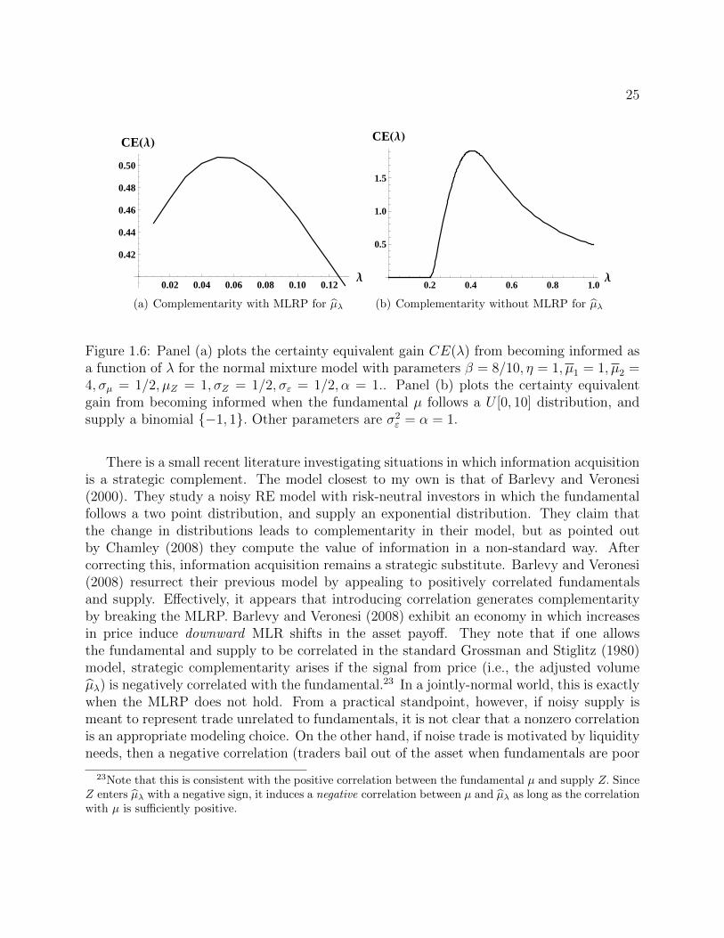
Example 1.4.1 (Failure of the MLRP is not necessary for complementarity). Figure 1.6(a)plots the certainty equivalent gain of becoming informed as a function of λ for a normalmixture example in which η = 1, so that the fundamental is not symmetric but supply issymmetric and normally distributed. The parameter values are those used in the backward-bending demand example in Section 1.4.1 above. Notice that the plot is increasing until λreaches about 0.05; over this region, information acquisition is a strategic complement. Dueto the normality of supply, this example satisfies the MLRP.

Example 1.4.2 (Failure of downward-sloping demand is not necessary for complementarity).Figure 1.6(b) plots the gain from becoming informed when the fundamental is distributeduniformly on [0, 10], and supply is drawn from a binomial distribution on {−1, 1} in whichboth realizations are equally likely. The binomial distribution for supply breaks the MLRP.22.In particular, for λ ≤ 1/5, the equilibrium is fully revealing, while for λ > 1/5, it is onlypartially revealing. This provides a stark illustration that without the MLRP, changes inthe fraction informed can have surprising effects on price informativeness.

22A two-point distribution for supply is not consistent with the standing assumption that all randomvariables are continuously distributed, but a similar result holds if one approximates the binomial distributionwith a continuous, ‘U’-shaped, distribution centered at zero and having peaks at −1 and 1.

25

0.02 0.04 0.06 0.08 0.10 0.12Λ

0.42

0.44

0.46

0.48

0.50

CEHΛL

(a) Complementarity with MLRP for µλ

0.2 0.4 0.6 0.8 1.0Λ

0.5

1.0

1.5

CEHΛL

(b) Complementarity without MLRP for µλ

Figure 1.6: Panel (a) plots the certainty equivalent gain CE(λ) from becoming informed asa function of λ for the normal mixture model with parameters β = 8/10, η = 1, µ1 = 1, µ2 =4, σµ = 1/2, µZ = 1, σZ = 1/2, σε = 1/2, α = 1.. Panel (b) plots the certainty equivalentgain from becoming informed when the fundamental µ follows a U [0, 10] distribution, andsupply a binomial {−1, 1}. Other parameters are σ2

ε = α = 1.

There is a small recent literature investigating situations in which information acquisitionis a strategic complement. The model closest to my own is that of Barlevy and Veronesi(2000). They study a noisy RE model with risk-neutral investors in which the fundamentalfollows a two point distribution, and supply an exponential distribution. They claim thatthe change in distributions leads to complementarity in their model, but as pointed outby Chamley (2008) they compute the value of information in a non-standard way. Aftercorrecting this, information acquisition remains a strategic substitute. Barlevy and Veronesi(2008) resurrect their previous model by appealing to positively correlated fundamentalsand supply. Effectively, it appears that introducing correlation generates complementarityby breaking the MLRP. Barlevy and Veronesi (2008) exhibit an economy in which increasesin price induce downward MLR shifts in the asset payoff. They note that if one allowsthe fundamental and supply to be correlated in the standard Grossman and Stiglitz (1980)model, strategic complementarity arises if the signal from price (i.e., the adjusted volumeµλ) is negatively correlated with the fundamental.23 In a jointly-normal world, this is exactlywhen the MLRP does not hold. From a practical standpoint, however, if noisy supply ismeant to represent trade unrelated to fundamentals, it is not clear that a nonzero correlationis an appropriate modeling choice. On the other hand, if noise trade is motivated by liquidityneeds, then a negative correlation (traders bail out of the asset when fundamentals are poor

23Note that this is consistent with the positive correlation between the fundamental µ and supply Z. SinceZ enters µλ with a negative sign, it induces a negative correlation between µ and µλ as long as the correlationwith µ is sufficiently positive.

26

and vice versa) may better fit our intuition.Ganguli and Yang (2009) demonstrate strategic complementarity in a CARA-normal

model in which investors can become informed about both the fundamental and aggregatesupply of the asset. When used in concert with the information in price, supply informationis valuable since it allows investors to more precisely ascertain whether the prevailing priceis due to the fundamental or merely a supply shock. With two dimensions of information,investors can coordinate on an equilibrium in which information acquisition is a strategiccomplement and price becomes less informative when the number of informed investors in-creases. If an additional trader becomes informed, the weight on the fundamental in the priceincreases. The increased weight on the fundamental makes all other investors trade moreintensely on their supply information, and if this effect is sufficiently strong, it can swampthe increased informativeness from the increased weight on the fundamental. Manzano andVives (2010) generalize the Ganguli and Yang (2009) setting to permit correlation betweensignal errors and demonstrate that strategic complementarity in the information market isnot robust, in that such equilibria are unstable in the multi-signal CARA-normal setting.

Other authors generate complementarity in models that differ more substantially fromthe one presented here. Chamley (2007) solves a sequential-trade model in which investorshave short horizons. In this setting, an increase in the number of informed investors drivestoday’s price closer to the fundamental, but can also make tomorrow’s price more uncertain.If the second effect is sufficiently strong, information acquisition can be a strategic comple-ment. Veldkamp (2006b) introduces an information production sector into an overlappinggenerations version of the standard Grossman and Stiglitz (1980) model. The endogenousprice of information generates complementarity in information acquisition and can lead to‘frenzies’ in the information market in which many investors seek to buy the same informa-tion. The information market is such that it costs the provider nothing to distribute theinformation once it has been discovered, so to maximize profits, she reduces the price ofinformation as demand increases to deter entry by competitors. Such price reduction canfeed back and further increase demand for information. In recent work, Garcıa and Strobl(2010) show that relative wealth concerns can generate complementarities in informationacquisition.

Despite these advances, to my knowledge, no one has yet demonstrated strategic com-plementarity in a standard static noisy REE model. Here, I have shown that even a simplemodel can generate the effect for purely informational reasons.

Implications for information market equilibria

Here I take up briefly the question of equilibrium in the information market, which wasdeferred from Section 1.2.1

In the examples presented in Figure 1.6 above, one can determine the equilibrium valueof λ for various values of c by drawing a horizontal ‘cost’ line at level c. Interior equilibria arepoints at which the cost line intersects the certainty equivalent gain, while corner equilibria

27

λ = 0 or 1 occur when CE(0) < c or CE(1) > c, respectively. In both examples in Figure1.6, there are multiple equilibria in the information market. First, there is a zero-informationequilibria in which no one finds it profitable to purchase information. Secondly, there aretwo interior equilibria24 in which a strictly positive number of agents gather information.This example is an illustration of the following Corollary to Proposition 1.4.4.

Corollary 1.4.5.

• If information acquisition is a strategic substitute for all λ ∈ (0, 1), then the equilibriumin the information market is unique.

• If information acquisition is a strategic complement for λ ∈ (0, k) for some constantk ∈ (0, 1), then there may exist multiple equilibria in the information market: forcertain values of c, there exist both an equilibrium in which no investors buy informationand interior equilibria in which a strictly positive number of investors buy information.

Since complementarity can generate multiple equilibria, my model, as those of Veldkamp(2006b) or Chamley (2007), provides a potential explanation for time-varying price informa-tiveness. If markets can jump between zero-information and positive-information equilibria,then the information content of price can change abruptly over time.

1.4.4 The relation between disagreement and returns

A number of empirical papers document a negative relation between investor disagreementand future returns (see, e.g., Diether, Malloy, and Scherbina, 2002; Goetzmann and Massa,2005).25 The “difference of opinions” (abbreviated DO) model of Miller (1977) in whichinvestors “agree to disagree” and do not condition on prices implies that if investors areshort-sale constrained then stocks about which there is more disagreement will tend to havehigher valuations (and hence lower returns). The reason is that the most pessimistic investorsare prevented from taking negative positions. Chen, Hong, and Stein (2002) build on theMiller (1977) insight and provide further empirical support. Accordingly, based on thesemodels, the documented negative relation between disagreement and returns is often takenas evidence that investors do not fully condition on prices

Banerjee (2010) points out the difficulty of distinguishing RE and DO models in a staticsetting with no short-sale constraints. Static RE and DO models can be made observationallyequivalent by appropriate parameter choices. To distinguish the hypotheses, Banerjee (2010)considers how disagreement relates to the dynamic properties of returns and trading volumein a setting in which investors care about future resale prices. His empirical results supportthe hypothesis that investors do in fact condition on prices on average.

24Only the interior equilibria at which CE is downward-sloping is stable in the tantonnement sense.25There is some contrary evidence from Doukas, Kim, and Pantzalis (2006), but most studies find a

negative relation.

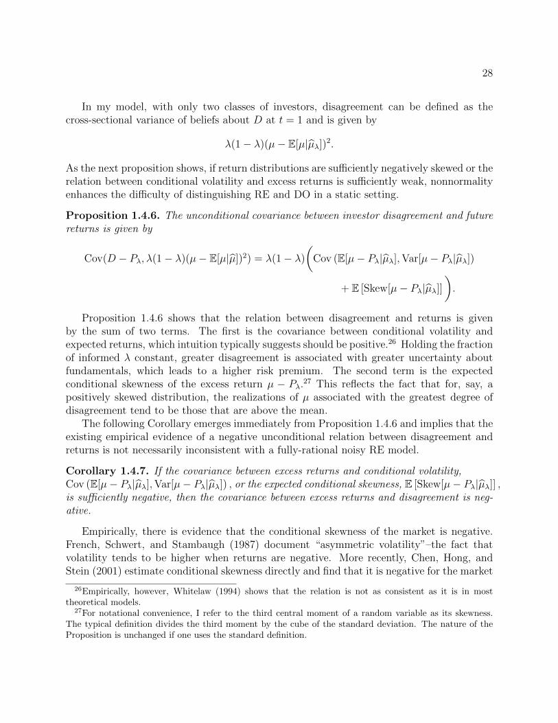
28

In my model, with only two classes of investors, disagreement can be defined as thecross-sectional variance of beliefs about D at t = 1 and is given by

λ(1− λ)(µ− E[µ|µλ])2.

As the next proposition shows, if return distributions are sufficiently negatively skewed or therelation between conditional volatility and excess returns is sufficiently weak, nonnormalityenhances the difficulty of distinguishing RE and DO in a static setting.

Proposition 1.4.6. The unconditional covariance between investor disagreement and futurereturns is given by

Cov(D − Pλ, λ(1− λ)(µ− E[µ|µ])2) = λ(1− λ)

(Cov (E[µ− Pλ|µλ],Var[µ− Pλ|µλ])

+ E [Skew[µ− Pλ|µλ]]).

Proposition 1.4.6 shows that the relation between disagreement and returns is givenby the sum of two terms. The first is the covariance between conditional volatility andexpected returns, which intuition typically suggests should be positive.26 Holding the fractionof informed λ constant, greater disagreement is associated with greater uncertainty aboutfundamentals, which leads to a higher risk premium. The second term is the expectedconditional skewness of the excess return µ − Pλ.

27 This reflects the fact that for, say, apositively skewed distribution, the realizations of µ associated with the greatest degree ofdisagreement tend to be those that are above the mean.

The following Corollary emerges immediately from Proposition 1.4.6 and implies that theexisting empirical evidence of a negative unconditional relation between disagreement andreturns is not necessarily inconsistent with a fully-rational noisy RE model.

Corollary 1.4.7. If the covariance between excess returns and conditional volatility,Cov (E[µ− Pλ|µλ],Var[µ− Pλ|µλ]) , or the expected conditional skewness, E [Skew[µ− Pλ|µλ]] ,is sufficiently negative, then the covariance between excess returns and disagreement is neg-ative.

Empirically, there is evidence that the conditional skewness of the market is negative.French, Schwert, and Stambaugh (1987) document “asymmetric volatility”–the fact thatvolatility tends to be higher when returns are negative. More recently, Chen, Hong, andStein (2001) estimate conditional skewness directly and find that it is negative for the market

26Empirically, however, Whitelaw (1994) shows that the relation is not as consistent as it is in mosttheoretical models.

27For notational convenience, I refer to the third central moment of a random variable as its skewness.The typical definition divides the third moment by the cube of the standard deviation. The nature of theProposition is unchanged if one uses the standard definition.

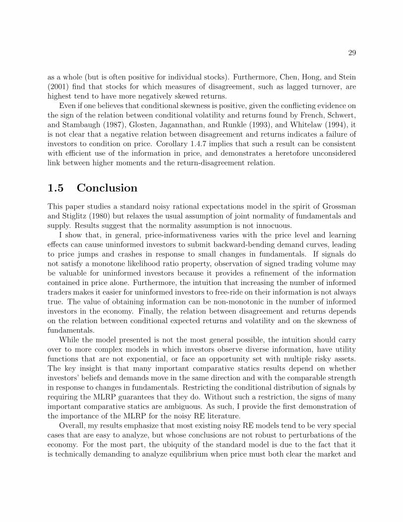
29

as a whole (but is often positive for individual stocks). Furthermore, Chen, Hong, and Stein(2001) find that stocks for which measures of disagreement, such as lagged turnover, arehighest tend to have more negatively skewed returns.

Even if one believes that conditional skewness is positive, given the conflicting evidence onthe sign of the relation between conditional volatility and returns found by French, Schwert,and Stambaugh (1987), Glosten, Jagannathan, and Runkle (1993), and Whitelaw (1994), itis not clear that a negative relation between disagreement and returns indicates a failure ofinvestors to condition on price. Corollary 1.4.7 implies that such a result can be consistentwith efficient use of the information in price, and demonstrates a heretofore unconsideredlink between higher moments and the return-disagreement relation.

1.5 Conclusion

This paper studies a standard noisy rational expectations model in the spirit of Grossmanand Stiglitz (1980) but relaxes the usual assumption of joint normality of fundamentals andsupply. Results suggest that the normality assumption is not innocuous.

I show that, in general, price-informativeness varies with the price level and learningeffects can cause uninformed investors to submit backward-bending demand curves, leadingto price jumps and crashes in response to small changes in fundamentals. If signals donot satisfy a monotone likelihood ratio property, observation of signed trading volume maybe valuable for uninformed investors because it provides a refinement of the informationcontained in price alone. Furthermore, the intuition that increasing the number of informedtraders makes it easier for uninformed investors to free-ride on their information is not alwaystrue. The value of obtaining information can be non-monotonic in the number of informedinvestors in the economy. Finally, the relation between disagreement and returns dependson the relation between conditional expected returns and volatility and on the skewness offundamentals.

While the model presented is not the most general possible, the intuition should carryover to more complex models in which investors observe diverse information, have utilityfunctions that are not exponential, or face an opportunity set with multiple risky assets.The key insight is that many important comparative statics results depend on whetherinvestors’ beliefs and demands move in the same direction and with the comparable strengthin response to changes in fundamentals. Restricting the conditional distribution of signals byrequiring the MLRP guarantees that they do. Without such a restriction, the signs of manyimportant comparative statics are ambiguous. As such, I provide the first demonstration ofthe importance of the MLRP for the noisy RE literature.

Overall, my results emphasize that most existing noisy RE models tend to be very specialcases that are easy to analyze, but whose conclusions are not robust to perturbations of theeconomy. For the most part, the ubiquity of the standard model is due to the fact that itis technically demanding to analyze equilibrium when price must both clear the market and

30

convey information (but not be fully-revealing). The assumptions of exponential utility andjoint normality ease the technical burden significantly and lead to a tractable, elegant model.However, a number of resulting properties that we take to be “properties of well-functioningfinancial markets” may be more appropriately considered to be “properties of the normaldistribution.”

31

1.6 Appendix

1.6.1 Some results on single-crossing and sign-regular functions

I collect in this Section some general results on single-crossing and sign-regular functionsthat are used to prove various results in the paper. I begin with the relevant definitions.

For my purposes, a single-crossing function is defined as follows.

Definition 1.6.1 (Single-crossing). A function f : R → R is single-crossing from below ifthere exists some point x0 such that x ≥ x0 implies f(x) ≥ 0. A function f is single-crossingfrom above if −f is single-crossing from below.

The following two definitions are taken directly from Definitions 1.1 and 1.2 in Chapter1 of Karlin (1968).

Definition 1.6.2 (Sign regularity). A function K : R2 → R is sign regular of order 2 (SR2)if there exist constants κ1, κ2 ∈ {−1, 1} such that κ1K(x, y) ≥ 0 and for for any choice ofx1 < x2 and y1 < y2

κ2

∣∣∣∣K(x1, y1) K(x1, y2)K(x2, y1) K(x2, y2)

∣∣∣∣ ≥ 0, (1.6)

where | · | represents the determinant. The function is strictly sign regular of order 2 (SSR2)if the inequalities are strict.

The more commonly-encountered property of total positivity is a special case of sign-regularity

Definition 1.6.3 (Total positivity). A function K : R2 → R is totally positive of order 2(TP2) if it is SR2 and κ1 = κ2 = 1. The function is strictly totally positive of order 2 (STP2)if it is SSR2 and κ1 = κ2 = 1.

To clarify the importance of sign regularity, recall that a conditional density fX|Y (x|y)has the (strict) MLRP if and only if it is (S)TP2. Similarly, a utility function u has (strictly)decreasing absolute risk aversion if and only if u′(x − y) is (S)TP2. Jewitt (1987, 1991)discusses these and other economic applications of sign regularity.

In the following Lemma, I generalize Theorem 11.2 from Chapter 6 Karlin (1968) tofunctions that are SR2. I also provide a “strong” version of the result for STP2 and SSR2

functions.

Lemma 1.6.1. Let f and K be functions mapping X×Y 7→ R for some intervals X, Y ⊂ R,and let µ be any σ-finite measure on Y. Assume that the integral g(x) :=

∫Yf(x, y)K(x, y)dµ(y)

exists and is continuous in x.If for each fixed y ∈ Y, f(x, y) is increasing in x, and either

32

(a) For each fixed x ∈ X, f(x, y) crosses zero at most once, and from below, as y increases,and K is TP2; or

(b) For each fixed x ∈ X, f(x, y) crosses zero at most once, and from above, as y increases,and K is SR2 with κ1 = 1, κ2 = −1;

then g crosses zero at most once, and from below, as x increases. (Note that the single-crossing “point” could in fact be an interval over which g = 0.) If the hypotheses are strength-ened to require that f is strictly increasing in x for fixed y and either (a) K is STP2, or(b) K is SSR2, then if g crosses zero it does so at a single point.

Proof of Lemma 1.6.1. I prove Case (b). First, consider the “weak” version of Case (b) inwhich K is SR2 and f is weakly increasing in x. The proof is similar to that of the weakversion of Case (a) in Karlin (1968). Take x0 such that g(x0) = 0. It suffices to show thatfor any x > x0, one has g(x) ≥ 0. By the hypothesis that f is single-crossing in y for fixed x,it follows that there exists y0 (which will, in general, depend on x0) such that f(x0, y) Q 0

as y R y0. Now, write

g(x)

K(x, y0)=

g(x)

K(x, y0)− g(x0)

K(x0, y0)

=

∫Yf(x, y)

K(x, y)

K(x, y0)dµ(y)−

∫Yf(x0, y)

K(x0, y)

K(x0, y0)dµ(y)

=

∫Y

(f(x, y)− f(x0, y))K(x, y)

K(x, y0)dµ(y) +

∫Yf(x0, y)

K(x, y)

K(x, y0)dµ(y)

−∫Yf(x0, y)

K(x0, y)

K(x0, y0)dµ(y)

=

∫Y

(f(x, y)− f(x0, y))K(x, y)

K(x, y0)dµ(y) +

∫Yf(x0, y)

[K(x, y)

K(x, y0)− K(x0, y)

K(x0, y0)

]dµ(y).

(1.7)

The first equality holds since g(x0) = 0, the second simply uses the definition of g to writeout the integrals, the next-to-last equality adds and subtracts f(x0, y) in first integral, andthe final line condenses the second and third integrals in the expression.

One can now use the expression in eq. (1.7) to sign g(x). Since f is increasing in x, the

term f(x, y) − f(x0, y) in the first integral is ≥ 0, and since κ1 = 1, one has K(x,y)K(x,y0)

≥ 0.

Thus, the first integral is ≥ 0. In the second integral, f(x0, y) Q 0 as y R y0 by the choice

of y0, and K(x,y)K(x,y0)

− K(x0,y)K(x0,y0)

Q 0 as y R y0 by the assumption that κ2 = −1. It follows that

the second integral is also ≥ 0. Hence, g(x)K(x,y0)

, and therefore g(x), is ≥ 0. This completes

the “weak” version of Case (b). The “strong” version follows immediately since in that case,the weak inequalities involving f and K that were used to sign the two integrals on the lastdisplayed line are strict.

33

For convenience, I restate, without proof, Lemma 1 from Persico (2000).

Lemma 1.6.2 (Lemma 1 from Persico (2000)). Let Y ⊂ R be any interval. Let g : R→ R bean increasing function, and let h : R→ R cross zero at most once and from below. Assumethat for some measure µ on Y, we have∫

Y

h(y) dµ(y) = 0.

Then, ∫Y

g(y)h(y) dµ(y) ≥ 0.

1.6.2 Proofs

I begin with two preliminary Lemmas that will be used in the proofs of Proposition 1.2.1and 1.2.4.

Lemma 1.6.3. If the uninformed investors can condition only in price, then any equilibriumprice function must be one-to-one in Z for each fixed realization µ = m and one-to-one in µfor each fixed realization Z = z.28

Proof of Lemma 1.6.3. I prove that price must be one-to-one in Z for fixed µ = m. The proofof the second result is essentially identical. Assume to the contrary that Pλ is an equilibriumprice function but that there exists some realization m such that Pλ(m, ·) is not one-to-onein its second argument. Then there exist realizations z 6= z′ with Pλ(m, z) = Pλ(m, z

′). Thisimplies

0 = (1− λ)XU(P (m, z)) + λm− Pλ(m, z)

ασ2ε

− z market clearing in state (m, z)

= (1− λ)XU(P (m, z′)) + λm− Pλ(m, z′)

ασ2ε

− z since Pλ(m, z) = Pλ(m, z′)

6= (1− λ)XU(P (m, z′)) + λm− Pλ(m, z′)

ασ2ε

− z′ since z 6= z′

= 0 market clearing in state (m, z′),

which is a contradiction.

28Of course, one can only make such statements up to a sets of Lebesgue measure zero. As in the body ofthe paper, I do not insist on such qualifications in this Section. It is straightforward but tedious to extendall proofs to be fully rigorous with respect to such measure-theoretic details.

34

Proof of Proposition 1.2.1. For clarity, I break the proof into steps. I begin by solving theagents’ optimization problems assuming that the uninformed can condition only on the price,and that they have conjectured some (continuously differentiable) price function satisfyingthe conditions in Lemma 1.6.3 that they use for updating their beliefs. Next, I imposemarket clearing and simplify the resulting expression to produce the an implicit functionthat characterizes a candidate price function. There are then two cases to consider, one inwhich the candidate price function satisfies the condition in Lemma 1.6.3 and one in which itdoes not. I verify that when the candidate function does satisfy the condition then observingadjusted volume provides no additional information beyond that conveyed by price alone,which completes the proof in this case. To conclude, I show that when the candidate functiondoes not satisfy the conditions Lemma 1.6.3, it nevertheless remains an equilibrium pricefunction as long as the uninformed can condition on adjusted volume.

Fix a realization of (µ, Z) = (m, z). Consider the informed agent’s maximization problem.

maxx∈R

E[− exp{−αx(D − Pλ)}|µ = m,Pλ = p].

Since this problem is that of a CARA investor facing a conditionally normal risky asset, thedemand function is standard

XI(m, p) =m− pασ2

ε

.

Next, consider an uninformed agent’s maximization problem. Assume that the unin-formed conjecture some price function Pλ : R2 → R when computing their posterior beliefsgiven the observed price p, and this function satisfies the condition in Lemma 1.6.3

maxx∈R

E[− exp{−αx(D − Pλ)}|Pλ = p].

Since ε is independent of the other random variables, I can integrate it out, rewriting themaximization as

maxx∈R

E[− exp{−αx(µ− Pλ) +1

2α2σ2

εx2}|Pλ = p].

Differentiation yields the first-order condition for uninformed demand XU(p).29 Since theutility function is strictly concave, the first-order condition defines the global maximum.

E[(µ− Pλ −XU(p)ασ2ε) exp{−αXU(p)(µ− Pλ) +

1

2α2σ2

ε (XU(p))2}|Pλ = p] = 0. (1.8)

29Differentiation through the expectation is justified since the expected utility is a conditional momentgenerating function of D evaluated at the point −αx, and moment generating functions are infinitely con-tinuously differentiable in their domain of existence.

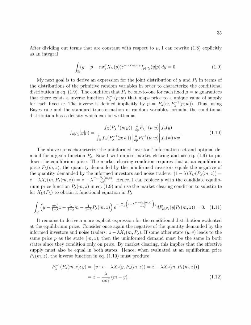
35

After dividing out terms that are constant with respect to µ, I can rewrite (1.8) explicitlyas an integral ∫

R(y − p− ασ2

εXU(p))e−αXU (p)yfµ|Pλ(y|p) dy = 0. (1.9)

My next goal is to derive an expression for the joint distribution of µ and Pλ in terms ofthe distributions of the primitive random variables in order to characterize the conditionaldistribution in eq. (1.9). The condition that Pλ be one-to-one for each fixed µ = w guaranteesthat there exists a inverse function P−1

λ (p;w) that maps price to a unique value of supplyfor each fixed w. The inverse is defined implicitly by p = Pλ(w,P

−1λ (p;w)). Thus, using

Bayes rule and the standard transformation of random variables formula, the conditionaldistribution has a density which can be written as

fµ|Pλ(y|p) =fZ(P−1

λ (p; y))∣∣∣ ∂∂pP−1

λ (p; y)∣∣∣ fµ(y)∫

R fZ(P−1λ (p;w))

∣∣∣ ∂∂pP−1λ (p;w)

∣∣∣ fµ(w) dw. (1.10)

The above steps characterize the uninformed investors’ information set and optimal de-mand for a given function Pλ. Now I will impose market clearing and use eq. (1.9) to pindown the equilibrium price. The market clearing condition requires that at an equilibriumprice Pλ(m, z), the quantity demanded by the uninformed investors equals the negative ofthe quantity demanded by the informed investors and noise traders: (1− λ)XU(Pλ(m, z)) =

z − λXI(m,Pλ(m, z)) = z − λm−Pλ(m,z)ασ2

ε. Hence, I can replace p with the candidate equilib-

rium price function Pλ(m, z) in eq. (1.9) and use the market clearing condition to substitutefor XU(Pλ) to obtain a functional equation in Pλ∫

R

(y − ασ2

ε

1−λz + λ1−λm−

11−λPλ(m, z)

)e− α

1−λ

(z−λm−Pλ(m,z)

ασ2ε

)ydFµ|Pλ(y|Pλ(m, z)) = 0. (1.11)

It remains to derive a more explicit expression for the conditional distribution evaluatedat the equilibrium price. Consider once again the negative of the quantity demanded by theinformed investors and noise traders: z− λXI(m,Pλ). If some other state (y, v) leads to thesame price p as the state (m, z), then the uninformed demand must be the same in bothstates since they condition only on price. By market clearing, this implies that the effectivesupply must also be equal in both states. Hence, when evaluated at an equilibrium pricePλ(m, z), the inverse function in eq. (1.10) must produce

P−1λ (Pλ(m, z); y) = {v : v − λXI(y, Pλ(m, z)) = z − λXI(m,Pλ(m, z))}

= z − λ

ασ2ε

(m− y) . (1.12)

36

It follows that the conditional density in eq. (1.10) can be written as

fµ|Pλ(y|Pλ(m, z)) =

fZ

(z − λ

ασ2ε

(m− y))fµ(y)

∣∣∣ ∂∂pP−1λ (p; y)

∣∣∣ ∣∣∣∣p=Pλ(m,z)∫

RfZ

(z − λ

ασ2ε

(m− w))fµ(w)

∣∣∣ ∂∂pP−1λ (p;w)

∣∣∣ ∣∣∣∣p=Pλ(m,z)

dw

. (1.13)

To eliminate the remaining Jacobian terms, differentiate eq. (1.12) totally with respect to zto obtain

∂

∂pP−1λ (p; y)

∣∣∣∣p=Pλ(m,z)

∂

∂zPλ(m, z) = 1,

which can be rearranged to yield ∂∂pP−1λ (p; y)

∣∣∣∣p=Pλ(m,z)

= 1∂∂zPλ(m,z)

. This expression is con-

stant with respect to y, so the Jacobian terms cancel from the numerator and denominatorof eq. (1.13). Substituting this conditional density into eq. (1.11), canceling terms that donot depend on y, and rearranging produces eq. (1.1) in the text.

If the function Pλ defined implicitly by (1.1) is in fact one-to-one in each variable whenthe other is held fixed, then the condition from Lemma 1.6.3 is met and Pλ is an equilibriumprice function for the case in which the uninformed can condition only on the asset price.Since the uninformed can also condition on the signed volume of the informed and noisetraders, then in principle Pλ may not remain an equilibrium. This would be the case if thesigned volume, λXI(m,Pλ)−z, reveals strictly more information that the linear combination,m, that is revealed by the price However, it does not do so. To see this, note that the signedvolume also depends (directly) on m and z only through m :

λXI(m,Pλ)− z = λm− Pλασ2

ε

− z

=λ

ασ2ε

(m− Pλ) (1.14)

This concludes the proof in the case that Pλ is monotone.If the function Pλ defined by (1.1) is not one-to-one in m for fixed z, then the inversion

in eq. (1.13) in the proof is not possible for all realizations p. Hence, if the uninformed cancondition only on the asset price, then equilibrium does not exist in this case. However,as long as the uninformed can condition on signed volume, then the (non-one-to-one) Pλfrom eq. (1.1) is still an equilibrium price function. To prove this, it suffices to show thatobserving the combination of Pλ from eq. (1.1) and signed volume is equivalent to observingm. Hence, the uninformed investors’ updating step in eq. (1.13) will still reduce to updat-ing from observations of the random variable µλ. Given the signed volume can be written

37

as in eq. (1.14), the required observational equivalence is immediately apparent since the

uninformed need only to multiply the signed volume by ασ2ε

λand add Pλ to obtain m. This

completes the proof.

Proof of Proposition 1.2.3. Fix any realization µλ = m. Suppose that the conditional mo-ment generating function of µ given µλ = m exists in some open interval (−δ0, ζ0), whereδ0, ζ0 > 0, allowing the possibility of either endpoint being ∞. Consider eq. (1.2) as a func-

tion of p, after multiplying by e− λ

1−λm−pσ2ε

m, which is constant with respect to y and strictly

positive, and thus does not affect the value of p at which eq. (1.2) equals zero

F (p) :=

∫R

((1− λ)y + λm− p) eλ

1−λm−pσ2ε

(y−m)fµ|µλ(y|m) dy.

If this integral exists and is continuous in p in some nonempty open set, then by the inter-mediate value theorem, it suffices to show that there exist p and p′ in that open set suchthat F (p) < 0 and F (p′) > 0.

Given the assumption on existence of the conditional moment-generating function, theintegral is finite as long as p satisfies λ

1−λm−pσ2ε∈ (−δ0, ζ0). Furthermore, since moment gen-

erating functions are infinitely continuously differentiable in their domain of existence, itfollows that F is continuously differentiable in p.30 It remains to find the p and p′ withF (p) < 0 and F (p′) > 0.

Evaluating F at m gives

F (m) = (1− λ)

∫R(y − m)fµ|µ(y|m) dy.

If E[µ|µλ = m] = m, existence is thus immediate, with Pλ(m) = m. If such is not thecase, then the sign of F (m) depends on whether the conditional expectation of µ givenµλ = m is greater or less than m itself. Without loss of generality, consider the case in whichE[µ|µλ = m] > m. Then, F (m) > 0. It remains to find p such that F (p) < 0.

Parameterize p(δ) = m + σ2ε

1−λλδ, where 0 < δ < δ0. I will show that one can choose δ

such that F (p(δ)) < 0. We have

F (p(δ)) = (1− λ)

∫R(y − m)e−δ(y−m)fµ|µ(y|m) dy − σ2

ε

1− λλ

δ

∫Re−δ(y−m)fµ|µ(y|m) dy

< (1− λ)

∫R(y − m)e−δ(y−m)fµ|µ(y|m) dy.

30To see this, let Mµ|µλ denote the conditional moment generating function and write F as

F (p) =

[(1− λ)M ′µ|µλ

(λ

1−λm−pσ2ε

∣∣∣∣m)+ (λm− p)Mµ|µλ

(λ

1−λm−pσ2ε

∣∣∣∣m)] e− λ1−λ

m−pσ2ε

m.

38

Now, split the integral on the last line into positive and negative parts∫R(y − m)e−δ(y−m)fµ|µ(y|m) dy

=

∫R

1{y<m}(y − m)e−δ(y−m)fµ|µ(y|m) dy +

∫R

1{y≥m}(y − m)e−δ(y−m)fµ|µ(y|m) dy

≤∫R

1{y<m}(y − m)e−δ(y−m)fµ|µ(y|m) dy +

∫R

1{y≥m}(y − m)fµ|µ(y|m) dy. (1.15)

If the first integral in line (1.15) can be made arbitrarily negative by appropriate choiceof δ, it will dominate the second (positive) integral, and the proof will be complete. Itis convenient, and equivalent, to show that the negative of the first integral,

∫R−(y −

m)1{y<m}e−δ(y−m)fµ|µ(y|m) dy, can be made arbitrarily large. Consider first the case in

which δ0 = ∞. As δ → ∞, the integrand converges almost everywhere to ∞. Hence, byFatou’s Lemma, one has

lim infδ→∞

∫R−(y − m)1{y<m}e

−δ(y−m) dy ≥ ∞.

Thus, there exists some δ > 0 such that F (p(δ)) < 0, which completes the proof. Next,consider the case in which the moment generating function diverges at −δ0 for δ0 < ∞.Then, for δ ∈ (0, δ0), one has∫

R−(y − m)1{y<m}e

−δ(y−m) dy ≥∫R−(y − m)1{y<m−1}e

−δ(y−m) dy

≥∫R

1{y<m−1}e−δ(y−m) dy.

Let δ ↑ δ0. Because the moment generating function diverges at −δ0, it follows that

limδ↑δ0

∫R

1{y<m−1}e−δ(y−m) dy =∞.

Hence,

lim infδ↑δ0

∫R−(y − m)1{y<m}e

−δ(y−m) dy ≥ ∞,

which again guarantees the existence of δ > 0 such that F (p(δ)) < 0.

Proof of Proposition 1.2.4. To prove uniqueness in the case that the uninformed can condi-tion only on price, it suffices to show that the price correspondence defined by eq. (1.2) issingle-valued since the proof of Proposition 1.2.1 implied that in this case, any equilibrium

39

must be characterized by eq. (1.2). In the case that the uninformed can also condition onsigned volume, to show uniqueness among µλ-measurable price functions one must also showthat any such price function is characterized by eq. (1.2).

I begin by showing that the price correspondence defined by eq. (1.2) is single-valued.Fix µλ = m and apply Lemma 1.6.1 to∫

R− ((1− λ)y + λm− p) e

λ1−λ

m−pσ2ε

yfZ

(λ

ασ2ε

(y − m)

)fµ(y) dy, (1.16)

which is simply eq. (1.2) multiplied by −1 (this multiplication, of course, does not affect

the point p at which the expression equals zero). Since eλ

1−λµλ−pσ2ε

yis SSR2 in (p, y) and

−((1−λ)y+λµλ−p) is strictly increasing in p and single-crossing from above in y it followsthat (1.16) crosses zero at most once, at a single point, and from below, as p increases.

To prove that eq. (1.2) characterizes all µλ-measurable price functions, note that in theproof of Proposition 1.2.1, I showed that observation of a µλ-measurable price function alongwith signed volume provides the uninformed with the same information as direct observationof µλ. Hence, any such equilibrium is equivalent to one in which the uninformed conditiononly on µλ. Eq. (1.2) characterizes exactly this equilibrium.

Proof of Lemma 1.3.1. This result is well-known, and follows immediately after writing outfµλ|µ in terms of the density of supply fZ .

fµλ|µ(m|m) =λ

ασ2ε

fZ

(λ

ασ2ε

(m− m)

). (1.17)

The next lemma collects some useful expressions for the derivatives of uninformed demandand equilibrium price with respect to various quantities, assuming that the derivatives exist.

Lemma 1.6.4. Considered as a function of the realizations µλ = m and Pλ = p, the deriva-tives of uninformed demand XU are

∂XU

∂m=

∫R (y − p− ασ2

εXU) e−αXUy∂fµ|µ∂m

(y|m)

fµ|µ(y|m)fµ|µ(y|m) dy

α∫R [(y − p− ασ2

εXU) y + σ2ε ] e−αXUyfµ|µ(y|m) dy

(1.18)

∂XU

∂p=

−∫R e−αXUyfµ|µ(y|m) dy

α∫R [(y − p− ασ2

εXU) y + σ2ε ] e−αXUyfµ|µ(y|m) dy

. (1.19)

The derivatives of the price function Pλ with respect to the realization of µλ = m and the

40

parameter λ are

∂Pλ∂m

=

∫R [(1− λ)y + λm− Pλ] e

λ1−λ

m−Pλσ2ε

y∂fµ|µλ∂m

(y|m)

fµ|µλ (y|m)fµ|µλ(y|m) dy∫

R

([(1− λ)y + λm− Pλ] λ

1−λyσ2ε

+ 1)e

λ1−λ

m−Pλσ2ε

yfµ|µλ(y|m) dy

(1.20)

+

∫R

([(1− λ)y + λm− Pλ] λ

1−λyσ2ε

+ λ)e

λ1−λ

m−Pλσ2ε

yfµ|µλ(y|m) dy∫

R

([(1− λ)y + λm− Pλ] λ

1−λyσ2ε

+ 1)e

λ1−λ

m−Pλσ2ε

yfµ|µλ(y|m) dy

and

∂Pλ∂λ

=

∫R ((1− λ)y + λm− Pλ) e

λ1−λ

m−Pλσ2ε

y∂fµ|µλ∂λ

(y|m)


R

([(1− λ)y + λm− Pλ] λ

1−λyσ2ε

+ 1)e

λ1−λ

m−Pλσ2ε

yfµ|µλ(y|m) dy

(1.21)

+

m−Pλσ2ε(1−λ)2

∫R ((1− λ)y + λm− Pλ) ye

λ1−λ

m−Pλσ2ε


R

([(1− λ)y + λm− Pλ] λ

1−λyσ2ε

+ 1)e

λ1−λ

m−Pλσ2ε

yfµ|µλ(y|m) dy

+m−Pλ1−λ

∫R e

λ1−λ

m−Pλσ2ε


R

([(1− λ)y + λm− Pλ] λ

1−λyσ2ε

+ 1)e

λ1−λ

m−Pλσ2ε

yfµ|µλ(y|m) dy

.

Proof of Lemma 1.6.4. The first-order condition defining XU(m, p) is∫R

(y − ασ2

εXU − p)e−αXUyfµ|µλ(y|m) dy = 0.

The denominators in the expressions in the Lemma are non-zero due to Lemma 1.6.2. Hence,we can apply the implicit function theorem to obtain the results for ∂XU

∂mand ∂XU

∂pimmedi-

ately.Using the implicit function theorem on eq. (1.2), gives the results for ∂Pλ

∂m. Applying the

41

implicit function theorem again for ∂Pλ∂λ

gives

∂Pλ∂λ

=

∫R ((1− λ)y + λm− Pλ) e

λ1−λ

m−Pλσ2ε

y∂fµ|µ∂λ

(y|m)


R

([(1− λ)y + λm− Pλ] λ

1−λyσ2ε

+ 1)e

λ1−λ

m−Pλσ2ε

yfµ|µ(y|m) dy

+

1(1−λ)2

m−Pλσ2ε

∫R ((1− λ)y + λm− Pλ) ye

λ1−λ

m−Pλσ2ε


R

([(1− λ)y + λm− Pλ] λ

1−λyσ2ε

+ 1)e

λ1−λ

m−Pλσ2ε

yfµ|µ(y|m) dy

−∫R (y − m) e

λ1−λ

m−Pλσ2ε


R

([(1− λ)y + λm− Pλ] λ

1−λyσ2ε

+ 1)e

λ1−λ

m−Pλσ2ε

yfµ|µ(y|m) dy

.

However, by rearranging eq. (1.2) one can see that

−∫R

(y − m) eλ

1−λm−Pλσ2ε

yfµ|µλ(y|m) dy =

m− Pλ1− λ

∫Re

λ1−λ

m−Pλσ2ε

yfµ|µλ(y|m) dy.

Substituting this for the numerator in the last term above gives the desired result.

Proof of Proposition 1.4.1. Under the assumption that fµλ|µ has the MLRP, Proposition1.4.2 below implies that the price function is invertible. This implies that uninformed demandis in fact a function of Pλ. Given that Pλ is increasing in µλ, is follows also that uninformeddemand will be increasing in price if and only if it is increasing in m. Assuming that the priceand uninformed demand functions are differentiable, differentiating the equilibrium demandXU(m, Pλ(m)) totally with respect to m gives

d

dmXU(m, Pλ(m)) =

∂XU

∂m+∂XU

∂p

∂Pλ∂m

.

Substitute in from Lemma 1.6.4 for all three partial derivatives on the right-hand side of theequation. It is then tedious but straightforward to manipulate the resulting expression andshow that it is ≥ 0 if and only if ∂Pλ

∂m≥ 1.

To prove the second statement, it suffices to show that logconcavity of fµ implies that∂Pλ∂m≤ 1. The nondifferentiable case can be handled by rearranging the uninformed first-order

condition and applying Corollary 2.3 of Ma (1999).Consider the expression for the derivative of the price function in eq. (1.20) By a simple

application of Bayes rule on the conditional density in the integrand, one can express the

42

numerator in the first term in eq. (1.20) as∫R

[(1− λ)y + λm− Pλ] eλ

1−λm−Pλσ2ε

y ∂fµλ|µ∂m

(m|y)fµ(y) dy (1.22)

From eq. (1.17), it follows that∂fµλ|µ∂m

(m|y) = −∂fµλ|µ∂y

(m|y). Use this fact to perform integra-

tion by parts on eq. (1.22) to obtain the following expression (the boundary terms are zerosince the densities have mgfs, and therefore tails that converge to zero at least exponentially)

= (1− λ)

∫Re

λ1−λ

m−Pλσ2ε

yfµλ|µ(m|y)fµ(y) dy +

λ

1− λm− Pλσ2ε

∫R

[(1− λ)y + λm− Pλ] eλ

1−λm−Pλσ2ε

yfµλ|µ(m|y)fµ(y) dy

+

∫R

[(1− λ)y + λm− Pλ] eλ

1−λm−Pλσ2ε

yfµλ|µ(m|y)

f ′µ(y)

fµ(y)fµ(y) dy.

The second term in this sum vanishes, due to the price equation eq. (1.2). Plugging theremaining two terms back into eq. (1.20) and rearranging gives

∂Pλ∂m

= 1 +

∫R [(1− λ)y + λm− Pλ] e

λ1−λ

m−Pλσ2ε

y f ′µ(y)

fµ(y)fµλ|µ(m|y)fµ(y) dy∫

R

([(1− λ)y + λm− Pλ] λ

1−λyσ2ε

+ 1)e

λ1−λ

m−Pλσ2ε

yfµλ|µ(m|y)fµ(y) dy

. (1.23)

If log fµ is concave, thenf ′µ(y)

fµ(y)is decreasing in y. The numerator of the second term in

eq. (1.23) is therefore ≤ 0 by Lemma 1.6.2, and as noted in the first section of this proof,the denominator is ≥ 0. Hence, the entire term is ≤ 0, and therefore ∂Pλ

∂m≤ 1.

Proof of Proposition 1.4.2. It suffices to show that under the MLRP the price function isstrictly increasing in the realization of µλ and hence invertible. I do so by showing that thederivative in eq. (1.20) is greater than zero.

From eq. (1.2) we know that [(1− λ)y + λm− Pλ] eλ

1−λm−Pλσ2ε

yintegrates to 0 against fµ|µ.

Furthermore, this function crosses zero once, and from below, as y increases. Since the MLRP

guarantees that∂fµ|µ∂m

(y|m)

fµ|µ(y|m)is increasing in y, Lemma 1.6.2 implies that the numerator of the

first term in eq. (1.20) is greater than zero. Similarly, since y is increasing, the numeratorof the second term and the denominator of each term are also greater than zero. It followsthat eq. (1.20) is greater than zero.

Proof of Lemma 1.4.3. Fix λ ∈ (0, 1), and choose any τ ∈ (λ, 1). Following Persico (1996,2000), define the function Tλ,τ,m(m) = m+ λ

τ(m−m). Persico (1996) shows that conditional

on µ = m the random variable µτ is equal in distribution to Tλ,τ,m(µλ). Hence, when fraction

43

τ are informed, the difference in certainty equivalent wealth is

CE(τ) = − 1

αlog

∫∫R2

e−αXI(m−Pτ )+12α

2X2Iσ

2εfµτ |µ(m|m)fµ(m) dmdm

+1

αlog

∫∫R2

e−αXU (m−Pτ )+ 12α

2X2Uσ

2εfµτ |µ(m|m)fµ(m) dmdm

= − 1

αlog

∫∫R2

eαc−αXI(m,Pτ (T (m)))(m−Pτ (T (m))+ 12α

2X2I (m,Pτ (T (m)))σ2

εfµλ|µ(m|m)fµ(m) dmdm

+1

αlog

∫∫R2

e−αXU (T (m),Pτ (T (m)))(m−Pτ (T (m))+ 12α

2X2U (T (m),Pτ (T (m)))σ2

εfµλ|µ(m|m)fµ(m) dmdm.

Differentiate this expression with respect to τ and evaluate the derivative at τ = λ. Sincethe integrand is continuously differentiable in τ, it is permissible to differentiate through theintegral sign.

d

dτCE(τ)

∣∣∣∣τ=λ

= − 1

αEI

∫∫R2

ddτ e

αc−αXI(m,Pτ (T (m)))(m−Pτ (T (m))+ 12α

2X2I (m,Pτ (T (m)))σ2

ε

∣∣∣∣τ=λ

fµλ|µ(m|m)fµ(m) dmdm

+1

αEU

∫∫R2

ddτ e−αXU (T (m),Pτ (T (m)))(m−Pτ (T (m))+ 1

2α2X2

U (T (m),Pτ (T (m)))σ2ε

∣∣∣∣τ=λ

fµλ|µ(m|m)fµ(m) dmdm,

where

EI = E[e−αXI(m−Pλ)+

12α

2X2Iσ

2ε

],

EU = E[e−αXU (m−Pλ)+ 1

2α2X2

Uσ2ε

]are the negative of the unconditional expected utilities of each type of investor.

I now proceed to differentiate the integrand. To conserve space, I use the notation eI

and eU for the exponentials in the informed and uninformed expected utility, divided by EIand EU, respectively.

= −∫∫

R2

{XI(m,Pτ (T (m)))

[∂Pτ∂m

∂T∂τ

+ ∂Pτ∂τ

]+(m− Pτ (T (m))− αXI(m,Pτ (T (m)))σ2

ε

) [ ∂XI∂p

[∂Pτ∂m

∂T∂τ

+ ∂Pτ∂τ

]+ ∂XI

∂τ

]}eI∣∣∣∣τ=λ

fµλ|µfµ dmdm

+

∫∫R2

{XU (T (m), Pτ (T (m)))

[∂Pτ∂m

∂T∂τ

+ ∂Pτ∂τ

]−(m− Pτ (T (m))− αXU (T (m), Pτ (T (m)))σ2

ε

) [ ∂XU∂m

∂T∂τ

+ ∂XU∂p

[∂Pτ∂m

∂T∂τ

+ ∂Pτ∂τ

]+ ∂XU

∂τ

]}eU∣∣∣∣τ=λ

fµλ|µfµ dmdm.

The informed investors’ first-order condition implies that

m− Pτ (T (m))− αXI(m,Pτ (T (m)))σ2ε = 0,

which eliminates the second term in the first integral. Similarly, the uninformeds’ first-ordercondition implies that the terms in the second integral involving ∂XU

∂p× ∂Pτ

∂τand ∂XU

∂τvanish

44

when integrating over m since these expressions depend only on m. Hence, the expressionbecomes

= −∫∫

R2

XI(m,Pτ (T (m)))[∂Pτ∂m

∂T∂τ + ∂Pτ

∂τ

]eI∣∣∣∣τ=λ

fµλ|µfµ dmdm

+

∫∫R2

{XU (T (m), Pτ (T (m)))

[∂Pτ∂m

∂T∂τ + ∂Pτ

∂τ

]−(m− Pτ (T (m))− αXU (T (m), Pτ (T (m)))σ2

ε

) [∂XU∂m + ∂XU

∂p∂Pτ∂m

]∂T∂τ

}eU∣∣∣∣τ=λ

fµλ|µfµ dmdm.

Finally, substitute for ∂T∂τ

and use the fact that Tλ,λ,m(m) = m to evaluate the integrandexplicitly at τ = λ to derive the expression in the text,

CE′(λ) = −∫∫

R2

(XI(m,Pλ(m))eI −XU (m, Pλ(m))eU

) [∂Pλ∂m

m−mλ + ∂Pλ

∂λ

]fµλ|µfµ dmdm

−∫∫

R2

(m− Pλ(m)− αXU (m, Pλ(m))σ2

ε

) [∂XU∂m + ∂XU

∂p∂Pλ∂m

]m−mλ

}eUfµλ|µfµ dmdm.

Proof of Proposition 1.4.4. The expression I desire to sign is

−∫∫

R2

(m− Pλ(m)− αXU(m, Pλ(m))σ2ε)[∂XU∂m

+ ∂XU∂p

∂Pλ∂m

]m−mλ

}eUfµ|µλfµλ dmdm.

(1.24)

Note that ∫R

(m− Pλ(m)− αXU(m, Pλ(m))σ2

ε

)eUfµ|µλ dm = 0

from the uniformed investors’ first order condition. Given that m − m is increasing in m,Lemma 1.6.2 will once again imply that the inner integral in eq. (1.24) (and hence the

entire expression) is ≥ 0 as long as[∂XU∂m

+ ∂XU∂p

∂Pλ∂m

]≤ 0 for all m. However, the proof of

Proposition 1.4.1 shows that this is the case if and only if uninformed demand is everywheredownward-sloping. Hence, under this assumption eq. (1.24) is ≥ 0.

Proof of Corollary 1.4.5. Interior equilibria in the information market are defined as λ∗ suchthat CE(λ∗) = c, and zero-information-acquisition equilibria, λ∗ = 0, occur when CE(0) ≤ c.Therefore, if CE is nonmonotonic, then for appropriate c there can be multiple values of λ∗,including zero, consistent with equilibrium.

Proof of Proposition 1.4.6. Using the law of total covariance and the fact that ε is indepen-

45

dent of all other random variables, write

Cov(D − Pλ, (µ− E[µ|µλ])2

)= Cov

(E [µ− Pλ|µλ] ,E[(µ− E[µ|µλ])2|µλ]

)+ E

[Cov

(µ− Pλ, (µ− E[µ|µλ])2|µλ

)]= Cov (E [µ− Pλ|µλ] ,Var[µ||µλ]) + E

[Cov

(µ− Pλ, (µ− E[µ|µλ])2|µλ

)]= Cov (E [µ− Pλ|µλ] ,Var[µ|µλ]) + E

[Cov

(µ− E[µ|µλ], (µ− E[µ|µλ])2|µλ

)]= Cov (E[µ− Pλ|µλ],Var[µ|µλ]) + E [Skew[µ|µλ]] .

The second equality uses the definition of conditional variance to simplify the first term.The third inequality uses the fact that Pλ and E[µ|µλ] are conditionally constant to manip-ulate the conditional covariance in the second term. The last equality uses the fact thatE[µ − E[µ|µλ]] = 0 to rewrite Cov (µ− E[µ|µλ], (µ− E[µ|µλ])2|µλ) = E[(µ − E[µ|µλ])3|µλ].Multiplying the above expression by λ(1 − λ) and using the fact that the covariance is abilinear operator to pull this constant inside the expression gives the desired result.

Proof of Corollary 1.4.7. Follows immediately from Proposition 1.4.6.

46

Chapter 2

Do Fund Managers Make InformedAsset Allocation Decisions

Note: This chapter represents joint work with Jacob S. Sagi.

2.1 Introduction

Every active fund manager has to make asset allocation decisions, and changes in the portfolioweights of major asset classes should be viewed as a function of the manager’s informationset and her or her ability to optimally use that information set.1 This paper develops afully dynamic model of the asset allocation decision, where each portfolio manager accountsfor a historical time series of public and private information available to him or her. Suchinformation, if used optimally, will reflect itself in the dynamics of portfolio weights. Themodel leads to testable and, to our knowledge, novel predictions. The main prediction, aftersuitably controlling for the conditional volatility of market returns, is that aggregate equityweights that are more volatile reflect better information and should better forecast futuremarket returns.

We apply the model to the portfolio weights of US mutual funds holding primarily UScommon equity from 1979Q3 until 2006Q4. We find evidence for the model predictions atforecasting horizons from three to twelve months, but weak contrary evidence at one-monthforecasting horizons. The timing ability we find at horizons beyond one month is consistentwith a small number of recent studies, and we interpret it as indicative of better informationabout medium-term future market returns. If one believes our model assumptions andempirical methodology are sound, one can attribute the general absence of timing ability ata shorter horizons as evidence against the existence of much private information about short-run expected returns. However, even for forecasting horizons over which some managers

1The decision by an active manager to not attempt to time the market is also a decision that is presumablybased on the manager’s information.

47

appear to have ability, timing behavior does not reflect itself in higher returns on funds’portfolios. This could be because of measurement error or because the portfolios are notheld long enough to benefit from the predictability.

2.1.1 Literature review and motivation

The literature on portfolio management generally views ‘market timing’ as the shifting offunds between broad asset categories (such as ‘US equities’, or ‘US Government bonds’) inan attempt to capture higher risk-adjusted returns. Skillful market timers are said to divinethose times during which returns on one major asset class will exceed those of another.

Early tests of market timing ability were largely based on the regression methodologiesof Treynor and Mazuy (1966) and Henriksson and Merton (1981), and looked for a convexrelationship between fund-level returns and contemporaneous market returns. Results fromthese early experiments have largely shaped researchers’ perception that professional port-folio managers do not exhibit timing ability.2 This is despite the fact that such tests aresusceptible to numerous criticisms (see Ferson and Schadt, 1996; Goetzmann, Ingersoll, andIvkovic, 2000; Jagannathan and Korajczyk, 1986; Kothari and Warner, 2001). For instance,bias can result if a portfolio is rebalanced more frequently than the observation intervalsused in the test. In addition, the residuals may be highly non-normal and correlated acrossfunds, leading one to potentially question the use of pooled statistics employed by all theearly studies (this is similar to the criticism offered by Kosowski, Timmermann, Wermers,and White, 2006). Finally, even if managers possessed timing ability, one might not detect itusing fund-level returns because the latter incorporate fees which, in a competitive market,could offset the value added by market timing (e.g., Berk and Green, 2004). Ferson andSchadt (1996) also point out that market timing tests should condition on public informa-tion relevant to predicting the market. When making the appropriate modifications, thenegative results of earlier tests disappear and they even find weak support for timing ability,although their inference from pooled statistics does not account for cross-sectional correla-tions and non-normalilty when computing standard errors. Edelen (1999) confirms thesefindings, pointing out that fund flows account for the negative results obtained in earlierstudies.3

A number of subsequent studies have focused on holdings, often testing market timingin a multiple-asset allocation context. Those finding no evidence for timing include Daniel,Grinblatt, Titman, and Wermers (1997); Kacperczyk and Seru (2007); Kacperczyk, Sialm,and Zheng (2005); Kosowski, Timmermann, Wermers, and White (2006); Wermers (2000).4

2Among the early tests are Chang and Lewellen (1984); Henriksson (1984); Henriksson and Merton (1981);Kon (1983); Treynor and Mazuy (1966).

3Eckbo and Smith (1998) apply the conditional performance test approach of Ferson and Schadt (1996)to assess the performance of insiders on the Oslo Stock Exchange. They find no evidence of timing abilityamong these insiders.

4Recent related studies of mutual funds that employ holdings to construct performance measures include

48

Save for Kosowski, Timmermann, Wermers, and White (2006), these holding-based studiesemploy pooled statistics and, to our knowledge, do not fully adjust for the cross-sectionalcorrelation in funds’ weights when reporting significance. Such correlation may be partic-ularly important when testing for timing because funds presumably attempt to time thesame macroeconomic variables.5 Standing in contrast with the other holdings-based mutualfund studies of timing is Jiang, Yao, and Yu (2007), who estimate aggregate portfolio betasfrom mutual fund holdings and find that funds tend to hold higher beta securities prior towhen market returns are high. Taliaferro (2009), however, suggests that their results dependstrongly on the period 2000-2002 and that managers do not necessarily show timing abilitycontinuously over their sample. Recent work by Simutin (2009) finds a relation betweenforecasting ability and excess cash holdings of funds.

All of the studies mentioned thus far examine monthly and/or quarterly holdings. Severalrecent studies that examine timing ability at a higher frequency have tended to yield positiveevidence. Busse (1999) and Fleming, Kirby, and Ostdiek (2001) study volatility timing,while Chance and Hemler (2001) examine timing strategies based on the recommendationsof 30 Registered Financial Advisers that, when pooled, yield significant evidence for markettiming ability. The latter authors document that the use of daily data is key to theirfindings, confirming the negative results of Graham and Harvey (1996) who look at newsletterrecommendations on a monthly basis. Bollen and Busse (2001) also find significant evidencefor ability in their Treynor and Mazuy (1966) and Henriksson and Merton (1981) regressiontests using daily data and bootstrapped standard errors, although they do not control forcross-sectional correlations in their tests.

Overall, the picture that emerges from reviewing the literature is that early studies,though flawed, found no or negative evidence for timing ability, while a survey of recentliterature provides a substantially more mixed view of the topic. Of 14 mentioned paperswritten since the 1990’s on the subject of timing, seven find supportive evidence. By andlarge, there does not appear to be a definitive answer to whether the average portfoliomanager can create value through asset allocation. When one further considers that manyof the papers can potentially be criticized on econometric grounds, the picture becomeshazier still.

We attempt to shed additional light on this question by offering a new set of tests fortiming ability, and design our empirical methodology keeping in mind the various econometricpitfalls we’ve identified above. In addition, our tests address at least one additional issueignored in this literature: If market returns are forecasted to be higher than average but theSharpe Ratio is forecasted to be lower than average, it is not clear that a rational markettimer would elect to increase her exposure to equities. As far as we know, all of the studies

Huang, Sialm, and Zhang (2008) and Shumway, Szefler, and Yuan (2009).5While Kosowski, Timmermann, Wermers, and White (2006) use a bootstrap methodology, they only

mention their results for timing in a footnote without reporting their test methodology. It is therefore notclear how they controlled for cross-sectional correlations in market weights when conducting their bootstraptests for timing ability.

49

looking for market timing ability ignore the potential importance of conditional volatility onmarket timing, whereas this consideration plays a key role in our methodology.

2.1.2 Our contribution

We examine ‘market timing’ from several new perspectives. Consistent with the literature onthe predictability of aggregate returns, we assume that fund managers receive noisy privatesignals about future market returns.6 This information comes in two forms: informationabout the slow-moving expected equity premium, some of which is known to be present inmacroeconomic variables such as Lettau and Ludvigson’s (2001) cay; and information aboutthe shock to market returns.7 The first type of information provides the manager with arefined sense of the premium of the market over bonds, while the second type of informationcan provide the manager with more dramatic insight such as whether bonds may fare betterthan stocks in the immediate future. We also consider three types of managers. ‘Type 1’, ornon-highly informed, have access to private and public information about the slow movingequity premium, while ‘type 2’, or highly informed managers, in addition have access toinformation about the shock to market returns. Together, we refer to ‘type 1’ and ‘type 2’managers as informed managers. On the other hand, ‘type 3’, or noise traders, believe thatthey have access to information about the shock to market returns but in actuality observeonly noise. Correspondingly, we characterize the Bayesian-optimal changes in weights of thethree types of managers assuming they can invest in the market and/or in short-term bonds;the managers are assumed to optimize a mean-variance myopic objective function and cancondition on their current private information as well as all past private information, and allpast market returns.

The primary prediction of the model is that, controlling for conditional volatility, in-formed managers whose portfolio weight in equity exhibits a greater time-series variancemust possess better information. The reason is intuitive. A manager who has more preciseinformation will be able to take more extreme positions in response to her signals withoutincreasing the portfolio risk. Conversely, for noise traders, the greater the variance of port-folio equity weights, the less information about future market returns should be reflected

6The predictability of market returns has been documented in Breen, Glosten, and Jagannathan (1989);Campbell (2002); Campbell and Shiller (1988a,b); Keim and Stambaugh (1986); Lettau and Ludvigson(2001). The potential benefits from making use of this information in asset allocation decisions is docu-mented in, among other papers, Andrade, Babenko, and Tserlukevich (2006); Kandel and Stambaugh (1996);Whitelaw (1997). Because investors can rebalance their exposure to market risk in reaction to changes inpublicly available information, managers may not feel compelled to adjust their portfolio weights in reactionto such information. Thus it is better to view our managers’ information as private in this paper. In a sep-arate addendum, available upon request, we discuss and empirically compare publicly available predictorsof the equity premium to aggregate changes in funds’ equity weights. There, we also calculate the potentialutility loss to investors who ignore this predictability.

7We do not assume that the information about the slow-moving equity premium is public. In principal,such information can be correlated with public information.

50

in equity weights. This too is intuitive, a noise trader who believes that she has betterinformation will take more extreme positions, but in so doing she merely adds idiosyncraticnoise to her portfolio returns. In short, if managers have timing ability, we should observe apositive relation between the variability of portfolio weights and their forecasting power forfuture market returns, while if managers are trading mostly on noise, we should observe anegative relation.

The model also implies that the portfolio equity weights of every non-highly informedmanager ought to have an autocorrelation coefficient equal to that of the time-varying ex-pected equity premium. Roughly, the intuition for this result is that all non-highly in-formed managers are attempting to forecast the time-varying expected equity premium.Their Bayesian-optimal forecasts should, therefore, exhibit this very same persistence. Afurther implication is that the portfolio equity weights of highly informed managers andnoise traders will have a lower autocorrelation than a non-highly informed manager, andthat this autocorrelation will decrease with the signal-to-noise ratio of their high-frequencysignals. The intuition for this result is straightforward: information about the shock to themarket returns is, by definition, high frequency and iid. The more information that a man-ager has about the shock, the more her portfolio weights will respond to that information.Hence, for informed managers, the smaller the autocorrelation of a managers equity expo-sure, the more information she ought to have about future market returns, and this shouldbe reflected in the equity exposure of the fund.

The fact that our model is set in a partial equilibrium setting might invite criticism. Inparticular, in a general equilibrium setting the fact that all portfolio positions must sumto the ‘market’ precludes every investor from shifting weights with the equity premium.To address this, we first emphasize that, as in practice, managers in the model base theirtrades on a heterogeneous mix of public and private information and do not necessarilytilt their portfolios in the same direction. Second, we do not presuppose that informedfund managers span the entire market. Third, it is possible to embed a model of profitableinformed trading in a general equilibrium setting (see, for example, Grossman and Stiglitz,1980); to our knowledge, there is nothing in the model or the industrial organization of themutual fund industry that suggests that general equilibrium considerations will nullify themodel’s predictions.

The model predictions are made under the assumption that one can control for non-informational changes in portfolio weights (e.g., fund flows, or portfolio insurance strate-gies), and we attempt to do this in our empirical tests. While our predictions ought to befairly robust because the economic rationale behind them is more general than the particu-lar model we investigate, in our battery of empirical tests we focus on the relation betweenthe variability of portfolio equity weights and their market forecasting power. There area number of reasons to believe that the our predictions on weight autocorrelation will beless robust. If the market autocorrelation is low, even minor misspecification in our controlvariables may lead to spurious results. Additionally, to the extent that managers disagreeon the data generating process for market returns, it is difficult to interpret deviations from

51

the predictions. Conversely, the prediction relating weight variability and forecasting powerrelies only on the assumption of manager rationality, as long as a forecast that incorporatesa manager’s signal is more precise that one that does not. Nevertheless, the model used toderive our results is rich in allowing a great deal of heterogeneity in fund manager charac-teristics and their private information. We test the model predictions on a large panel ofUS mutual fund holdings, and are able to, at least partially, assess the degree to which assetallocation decisions reflect information.

Our tests support the hypothesis that at three-, six-, and 12-month forecasting horizons,the market forecasting power of funds’ weights does increase with the weights’ variance (aspredicted by the model). Thus, it appears that variation in timing ability does exist inthe cross-section of mutual fund managers, at least at quarterly forecasting horizons andbeyond. On the other hand, we find essentially no evidence of timing ability at a one-monthhorizon. Our findings appear broadly consistent with those of Jiang, Yao, and Yu (2007),who find evidence of timing ability at horizons of three and six months, but not at theone-month horizon. We confirm their findings with respect to portfolio betas in our sample.Nevertheless, further tests lead us to conclude that the forecasting power documented hereand by Jiang, Yao, and Yu (2007) does not translate into higher portfolio returns.

It is important, however, to temper our results by noting that the holdings data used inour empirical tests are generally limited to US equity holdings only. We have no informationon how funds invest outside of this asset class. Although our treatment of fund holdings isconsistent with that of other studies, these funds could in principal make use of instrumentssuch as index futures or high-yield bonds to change their effective equity exposure and ourstudy would not pick this up.8 Moreover, it is also possible that the reported portfolioholdings suffer from window dressing and do not truly reflect funds’ portfolio strategies.

Section 2.2 develops the model. Section 2.3 describes our data set, the empirical method-ology, and reports our tests of the model. Section 2.4 analyzes the extent to which forecastingability is associated with improved portfolio returns. Section 2.5 concludes.

2.2 A model of optimal market timing

We begin by considering a typical market-timing fund manager, identified by the index i,who receives a noisy private signal each period about the market risk premium and adjustsher portfolio accordingly. Our assumptions represent a rich information environment, bothacross managers and across time. Doing so enables us to achieve a level of realism and gen-erality beyond the typical static modeling of the asset allocation decision under asymmetricinformation.

8Koski and Pontiff (1999) and Almazan, Brown, Carlson, and Chapman (2004) document that few fundsuse derivatives.

52

The market’s excess return at date t+ 1 is assumed to be:

ret+1 = µ+mt + εt+1, (2.1)

where µ is the unconditional premium and mt is its publicly unobserved time-varying compo-nent. The empirical literature notes that market return volatility is predictable. Consistentwith this, we assume that εt+1 has an observable date-t conditional variance of σ2

εt.9

There are three broad classes of portfolio managers. All types receive a noisy signal aboutmt of the form:

sit = nit +mt, (2.2)

where i indexes the identity of the manager and nit is the noise component of the manager’ssignal. The signal sit, incorporates public information (available to all fund managers) aswell as private information about mt. Whereas managers in all classes receive a private signalof the form sit, only managers belonging to the second class receive an additional signal ofthe form,

qHit = eit + εt+1, (2.3)

that provides information about the shock variable εt+1. We will refer to this second type ofmanager as being highly informed (the first class of managers will be referred to as non-highlyinformed).10 For every highly informed manager the conditional variances of eit and εt+1

at date t have a ratio, denoted Rqi, that does not vary with time. That is to say, for thehighly-informed manager, the signal-to-noise ratio of qit is constant. Finally, there is a thirdclass of managers, called noise traders, who believe that they receive a signal like that of thehighly informed managers, but in actuality receive only noise. Specifically they update theirbeliefs as though they receive a signal of the form

qNit′= e′it + εt+1,

where the ratio of conditional variances of e′it and εt+1 is still denoted Rqi. However, the true‘signal’ is purely noise

qNit = eit,

where the ratio of conditional variances of eit and εt+1 is 1 + Rqi. This assumption on

9It appears realistic to assume that investors observe the conditional volatility of market returns (using,for example, the S&P500 volatility index). In other words, Var[ret+1|Pt] is observable, with Pt representing acommon knowledge (public) information set. Under the assumption that mt is independent of εt+1, assumingthe observability of σ2

εt presupposes that Var[mt+1|Pt] is separately observable.10There is no loss of generality in thinking of the non-highly informed managers as receiving a signal of

the form qHit where Var[eit] is arbitrarily large.

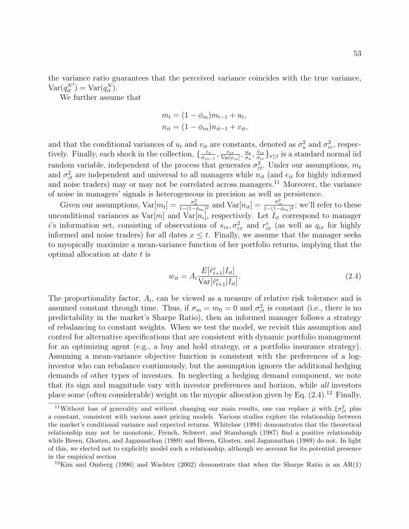
53

the variance ratio guarantees that the perceived variance coincides with the true variance,Var(qNit

′) = Var(qNit ).

We further assume that

mt = (1− φm)mt−1 + ut,

nit = (1− φin)nit−1 + vit,

and that the conditional variances of ut and vit are constants, denoted as σ2u and σ2

iv, respec-tively. Finally, each shock in the collection, { εs

σεs−1, eis

Var[eis], usσu, visσiv}s≤t is a standard normal iid

random variable, independent of the process that generates σ2εt. Under our assumptions, mt

and σ2εt are independent and universal to all managers while nit (and eit for highly informed

and noise traders) may or may not be correlated across managers.11 Moreover, the varianceof noise in managers’ signals is heterogeneous in precision as well as persistence.

Given our assumptions, Var[mt] = σ2u

1−(1−φm)2and Var[nit] =

σ2iv

1−(1−φin)2; we’ll refer to these

unconditional variances as Var[m] and Var[ni], respectively. Let Iit correspond to manageri’s information set, consisting of observations of six, σ

2εx and reix (as well as qix for highly

informed and noise traders) for all dates x ≤ t. Finally, we assume that the manager seeksto myopically maximize a mean-variance function of her portfolio returns, implying that theoptimal allocation at date t is

wit = AiE[ret+1|Iit]

Var[ret+1|Iit]. (2.4)

The proportionality factor, Ai, can be viewed as a measure of relative risk tolerance and isassumed constant through time. Thus, if σm = m0 = 0 and σ2

εt is constant (i.e., there is nopredictability in the market’s Sharpe Ratio), then an informed manager follows a strategyof rebalancing to constant weights. When we test the model, we revisit this assumption andcontrol for alternative specifications that are consistent with dynamic portfolio managementfor an optimizing agent (e.g., a buy and hold strategy, or a portfolio insurance strategy).Assuming a mean-variance objective function is consistent with the preferences of a log-investor who can rebalance continuously, but the assumption ignores the additional hedgingdemands of other types of investors. In neglecting a hedging demand component, we notethat its sign and magnitude vary with investor preferences and horizon, while all investorsplace some (often considerable) weight on the myopic allocation given by Eq. (2.4).12 Finally,

11Without loss of generality and without changing our main results, one can replace µ with ξσ2εt plus

a constant, consistent with various asset pricing models. Various studies explore the relationship betweenthe market’s conditional variance and expected returns. Whitelaw (1994) demonstrates that the theoreticalrelationship may not be monotonic, French, Schwert, and Stambaugh (1987) find a positive relationshipwhile Breen, Glosten, and Jagannathan (1989) and Breen, Glosten, and Jagannathan (1989) do not. In lightof this, we elected not to explicitly model such a relationship, although we account for its potential presencein the empirical section

12Kim and Omberg (1996) and Wachter (2002) demonstrate that when the Sharpe Ratio is an AR(1)

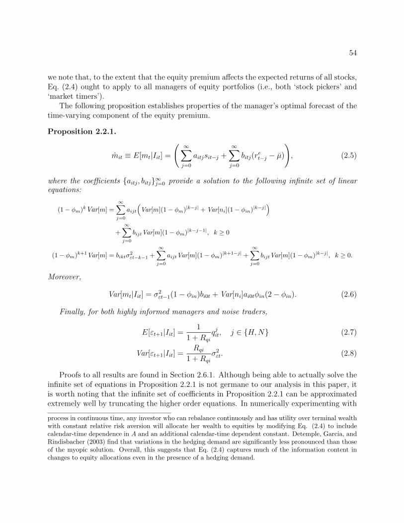
54

we note that, to the extent that the equity premium affects the expected returns of all stocks,Eq. (2.4) ought to apply to all managers of equity portfolios (i.e., both ‘stock pickers’ and‘market timers’).

The following proposition establishes properties of the manager’s optimal forecast of thetime-varying component of the equity premium.

Proposition 2.2.1.

mit ≡ E[mt|Iit] =

(∞∑j=0

aitjsit−j +∞∑j=0

bitj(ret−j − µ)

), (2.5)

where the coefficients {aitj, bitj}∞j=0 provide a solution to the following infinite set of linearequations:

(1− φm)kVar[m] =

∞∑j=0

aijt

(Var[m](1− φm)|k−j| + Var[ni](1− φin)|k−j|

)+

∞∑j=0

bijtVar[m](1− φm)|k−j−1|, k ≥ 0

(1− φm)k+1Var[m] = biktσ2εt−k−1 +

∞∑j=0

aijtVar[m](1− φm)|k+1−j| +

∞∑j=0

bijtVar[m](1− φm)|k−j|, k ≥ 0.

Moreover,

Var[mt|Iit] = σ2εt−1(1− φin)bi0t + Var[ni]ai0tφin(2− φin). (2.6)

Finally, for both highly informed managers and noise traders,

E[εt+1|Iit] =1

1 +Rqi

qjit, j ∈ {H,N} (2.7)

Var[εt+1|Iit] =Rqi

1 +Rqi

σ2εt. (2.8)

Proofs to all results are found in Section 2.6.1. Although being able to actually solve theinfinite set of equations in Proposition 2.2.1 is not germane to our analysis in this paper, itis worth noting that the infinite set of coefficients in Proposition 2.2.1 can be approximatedextremely well by truncating the higher order equations. In numerically experimenting with

process in continuous time, any investor who can rebalance continuously and has utility over terminal wealthwith constant relative risk aversion will allocate her wealth to equities by modifying Eq. (2.4) to includecalendar-time dependence in A and an additional calendar-time dependent constant. Detemple, Garcia, andRindisbacher (2003) find that variations in the hedging demand are significantly less pronounced than thoseof the myopic solution. Overall, this suggests that Eq. (2.4) captures much of the information content inchanges to equity allocations even in the presence of a hedging demand.

55

the equations, we’ve found that for realistic parameter settings it suffices to keep only thosecoefficients for which k ≤ 5.

2.2.1 Testable predictions

The next set of results pertains to the relation between the autocorrelation of funds’ equityportfolio weights and their associated forecasting power.

Proposition 2.2.2. The unconditional autocorrelation of Var[ret+1|Iit]×wit ∝ E[ret+1|Iit] fora non-highly informed manager is 1− φm, coinciding with the unconditional autocorrelationof mt.

Thus, controlling for the denominator in (2.4) (say, by multiplying wit by σ2εt and assuming

σ2εt � Var[mt|Iit]), the autocorrelation of the optimal weight assigned to the market is the

same across non-highly informed managers despite the rich heterogeneity in their informationstructure. One can understand the intuition for the result as follows: Every non-highlyinformed manager knows that the conditional equity premium has persistence of (1 − φm).If her estimate of the equity premium, mit, exhibits a different level of persistence, then themanager is either over-reacting or under-reacting to new information.

Corollary to Proposition 2.2.2. The unconditional autocorrelation of Var[ret+1|Iit] ×wit ∝ E[ret+1|Iit] for a highly informed manager or a noise trader is strictly smaller than1− φm, and monotonically decreases with 1

1+Rqi.

Recall that Rqi is the ratio of the conditional variances of eit to the conditional varianceof εt+1. A high value of 1

1+Rqiis therefore a measure of the signal-to-noise ratio of the

corresponding highly informed manager. The corollary states that a higher signal-to-noiseratio is associated with less persistence in E[ret+1|Iit]. Controlling for the denominator in(2.4), this implies that highly-informed managers and noise traders ought to exhibit lesspersistent equity portfolio weights. Putting together Propositions 2.2.2 and its corollary,one concludes that if managers are highly informed, the R2 in a regression of ret+1 againstVar[ret+1|Iit] × wit (a measure of forecasting power of fund weights) should monotonicallydecrease with the persistence of the portfolio equity weights. Conversely, if managers actas noise traders, the R2 should monotonically increase with the persistence of the portfolioequity weights.

As noted previously, Proposition 2.2.2 and its Corollary rely strongly on the assumptionthat the return generating process for ret+1 is common knowledge. Therefore, any tests ofthe Proposition or Corollary suffer from a joint hypothesis problem that managers both (1)agree on the return generating process and (2) use information optimally. As such, we refrainfrom attempting any direct tests of the Proposition or implications of its predictions.

The key result for our empirical tests relies on the observation that, controlling for thedenominator in (2.4), the time-series variation in weights is related to the quality of the

56

manager’s signal. If the quality of the signal is poor (e.g., consider a non-highly informed

manager with Var[m]Var[m]+Var[ni]

small), then the manager will optimally react by being careful not

to make dramatic changes in the weights, which are proportional to changes in E[ret+1|Iit].Likewise, a high quality signal will be associated with larger shifts in weights in response tothe signal. Thus, a higher variance of portfolio weights ought to reflect better forecastingpower for the market returns. This is the subject of the next result.

Proposition 2.2.3. For non-highly informed and highly informed managers, the regressionof ret+1 on E[ret+1|Iit] yields a slope coefficient of β = 1, and for noise traders the regressionyields a slope coefficient of β < 1. Moreover, the unconditional correlation of ret+1 withE[ret+1|Iit] is

ρrri = β

√√√√Var[E[ret+1|Iit]

]σ2r

=

σmiσr

if i is non-highly informed

σmiσr

√1 +

σ2εt

(1+Rqi)σ2mi

if i is highly informed

σmiσr

1√1+

σ2εt(1+Rqi)σ

2mi

if i is a noise trader,

(2.9)

where σr is the unconditional standard deviation of equity returns and σmi is the uncondi-tional standard deviation of mit.

An implication of Eq. (2.9) is that, controlling for the conditional volatility in Eq. (2.4),if managers have timing ability the R2 in a regression of the market excess return againstlagged realizations of Var[ret+1|Iit] × wit (i.e., ρ2

rmi) should be increasing in the time-series

varianceVar[Var[ret+1|Iit]×wit

]= Var

[E[ret+1|Iit]

]. Conversely, if managers act as noise traders, the

R2 should be decreasing in the above time-series variance.Unlike the predictions on weight autocorrelations, the prediction from Proposition 2.2.3

does not rely as strongly on fund managers agreeing on the data generating process. Rather,it essentially depends only on the assumption of individual rationality (as long as a forecastthat incorporates a manager’s signal is more precise than one that does not). Accordingly,it lends itself better to empirical testing, to which we turn in the next Section.

2.3 Empirical investigation

Our empirical work is guided by the model results of Section 2.2.1 where we assumed thatthe portfolio weight assigned to the market is given by Eq. (2.4). Before we can apply theresults of the model to open-end mutual funds holding domestic equity, we have to addressthree issues.

First, fund managers may not time the market by shifting between equities and cash.Rather, if a manager forecasts higher (lower) excess market returns in the near future, she

57

may move into (out of) high-beta stocks and leave her cash position unchanged. Even ifmanagers do time the market by adjusting cash holdings, the cash balance of the fund islikely to be affected by other factors not related to market timing, such as liquidity needsfor future redemptions.13 To account for these possibilities, we compute a holdings-basedportfolio beta for each fund at each report date and use the resulting beta, βit, as the‘effective’ portfolio weight in equities.14 In a setting in which a manager holds only cashand a market proxy, then the portfolio beta, of course, coincides with the raw weight in themarket proxy. To compute the holdings-based betas, we follow the procedure of Jiang, Yao,and Yu (2007), the details of which we outline in subsection 2.3.1 below.

A second issue is that managers may not follow a strategy that rebalances to constantweights in the absence of information. One example of this is a buy-and-hold strategy, whileanother is portfolio insurance. In the case of iid returns, it is well known (e.g., Cox andLeland, 2000; Leland, 1980) that these three dynamic strategic do not dominate each otherin the sense that certain investors (e.g., those exhibiting a particular version of decreasingrelative risk aversion) might prefer portfolio insurance while others might prefer a rebalancingstrategy. Moreover, in the presence of trading costs, it may be optimal to allow weights towander within an ‘inaction’ region (see Davis and Norman, 1990) and the optimal allocationof new funds might therefore exhibit a lag. Because all of these alternative reasons for weightchanges are contingent on past returns or fund flows, which are orthogonal to the error termin forecasting ret , one can still test the model by controlling for past returns and fund flows.

Finally, the Propositions pertain to the numerator of Eq. (2.4), but in practice portfolioweights incorporate the denominator as well:

wit =

Ai

µ+mitσ2εt+Var[mt|Iit]

if manager i is non-highly informed

Aiµ+mit+

qit1+Rqi

Rqi1+Rqi

σ2εt+Var[mt|Iit]

if manager i is highly informed or a noise trader.

(2.10)

Thus, in testing whether asset allocation is informed, one must control for the conditionalvolatility in the denominator of Eq. (2.10). To do so, we begin by assuming that

Rqi1+Rqi

σ2εt �

Var[mt|Iit], which appears reasonable given that the ‘shock’ component of market returns isharder to forecast than the equity premium and ought to vary substantially more.15 Based

13Chordia (1996) documents that fund cash holdings are affected by uncertainty over flows and the loadstructure of the fund, while Yan (2006) relates cash to the liquidity of funds’ holdings and to the level andvolatility of future flows. Simutin (2009) also documents a relation between excess cash holdings and theliquidity and riskiness of funds’ stock holdings.

14The betas we calculate have a correlation with the raw equity weights of only about 0.33, which suggeststhat the factors that affect cash holdings differ from those that affect portfolio allocation decisions.

15For example, even if the equity premium mt has a standard deviation of 4% per year, assuming thatRqi = 1, and that εt has an unconditional standard deviation of 16% per year, yields a ratio of

Rqi1+Rqi

σ2εt to

Var[mt|Iit] greater than 8.

58

on that assumption, one can approximate

σ2εtwit ≈

Ai

(µ+ mit

)if manager i is non-highly informed

Ai1+RqiRqi

(µ+ mit + qit

1+Rqi

)if manager i is highly informed or a noise trader.

(2.11)

One can proxy for σ2εt using a volatility index such as the vix, acknowledging that a

market forecast of volatility will differ, though likely not by much, from σ2εt.

16 Eq. (2.11)provides a proxy for Var[ret+1|Iit]×wit, and it is to this proxy that we will apply the insightsfrom Section 2.2.1.

2.3.1 Data

We obtain quarterly holdings information for all mutual funds, from 1979Q3 until 2006Q4,in the Thompson Financial CDA/Spectrum s12 database accessed through the Wharton Re-search Data Services (WRDS). The data is then linked to CRSP through WRDS’ MFLinksservice and the CRSP survivorship bias-free Mutual Fund Database (MFDB). For each quar-ter and each fund we obtain, whenever available, the portfolio weight corresponding to thetotal domestic equity holdings of the fund, the value-weighted return on those holdings in thethree months immediately following the report date, the S&P objective, style and specialtyfund codes (from CRSP MFDB), and the CDA/Spectrum s12 investment objective fundcode.17 We also obtain the return to fund investors, net of distributions, for each calendarquarter and document the dollar value of total assets managed by the fund. We augmentthis with quarterly data constructed from the monthly series of CRSP value-weighted re-turns and the risk-free rate (from WRDS), and quarterly data for the aggregate dividendyield and earnings-to-price ratio on the S&P500 index (Global Financial Data). Finally,our tests require a measure of conditional volatility, i.e., a proxy for σ2

εt. We compute fourdifferent such proxies of market volatilities: the first predictor is a naive monthly volatilitycalculated using the past month’s daily CRSP value-weighted return data, the second cor-responds to a fit of monthly CRSP value-weighted return data over the period 1954-2006to a GARCH(1,3) model, and the third consists of the S&P100 volatility index (vox from

16Var[ret+1|Pt], where Pt represents a common knowledge (public) information set, should be approximatelya constant proportion of Var[ret+1|Iit]. The deviation from a constant proportionality should amount to thedifference between Var[mt+1|Pt] and Var[mt+1|Iit], which ought to be small relative to σ2

εt.17Because funds report their holdings at different times, the holding returns are not contemporaneous

across all funds. When a fund reports holdings more than once in a quarter, we consider only the earliestreport for that quarter. Many funds only report twice a year, the minimum SEC requirement, resulting insubstantial ‘seasonality’ in the number of funds that report each quarter.

59

WRDS).18 The fourth proxy for σ2εt is a constant, corresponding to a situation in which fund

managers ignore changes in volatility when selecting the optimal equity position (the actualmagnitude of this constant is immaterial as it can be absorbed into Ai in the definition ofwit). In merging the volatility data with our quarterly observations, we choose the volatilitypredictor for the last month of each quarter.19

To compute holdings-based fund betas, we follow the procedure from Jiang, Yao, andYu (2007). Closing prices from CRSP are used to first calculate the portfolio weights of theindividual holdings of each fund on each reporting date.20 Denote by ωijt the weight of stockj in fund i’s portfolio at time t. Next, for each stock on each reporting date t, daily returnsfor the preceding one-year period are pulled from CRSP. The beta of stock j at date t iscomputed using the Dimson (1979) method. We run the regression

rejτ = ajt +5∑

q=−5

bjqtrem,τ−q + εjτ , τ ∈ {t− 364, t},

and the stock beta is estimated as the sum of the coefficients

bjt =5∑

q=−5

bjqt.

At least 60 daily return observations are required for this regression. Stocks not meetingthis criteria are assigned betas of one. All non-stock securities are assigned betas of zero.Combining the portfolio weights and stock beta estimates, the beta of fund i at time t isgiven by

βit =∑j

ωijtbjt.

We initially start with 5278 funds. We filter out funds that at any point reported anequity portfolio weight of more than 200% (76 funds), funds that report holdings in fewerthan eight quarters (983 more funds), and funds with an average equity portfolio weight of

18We found the GARCH(1,3) model to be the most parsimonious best fit nested within a GARCH(4,4)framework. Of the three, the GARCH measure is the only one that is incorporates information unavail-able contemporaneously because the coefficient estimates use the full time series. This turns out to beinconsequential for our tests.

19For the GARCH measure of volatility, while we could have used an average of the forecast for all threemonths of the quarter based on the last quarter’s information, this doesn’t significantly impact our testresults. Moreover, weights are typically reported towards the end of the quarter and would therefore reflecta volatility prediction for that month (given that turnover ratios for the average mutual fund tend to belarger than what might be suggested from reported quarterly weight changes).

20Individual stocks from the CDA/Spectrum s12 holdings file are matched with CRSP using CUSIPs and,when CUSIPs are not present in the holdings file, ticker symbols.

60

less than 50% (774 additional funds). We generally wish to investigate funds that invest ina broad enough range of domestic equity so that information about the US equity premiumought to particularly matter to them. Table 2.1 tabulates how the remaining 3445 funds arethen categorized as ‘broad domestic equity funds’ using their CDA/Spectrum s12 investmentobjective codes, ICDI (MFDB) objective codes, and S&P objective codes.21 Funds nothighlighted in the table are considered ‘broad domestic equity funds’. We exclude the otherfunds from the sample and are left with 2766 funds. Even for these remaining funds, somefields are missing for some (or all) quarters.

For each fund, we calculate the time-series average holdings-based beta, the averageweight of domestic equity in the fund’s portfolio, the average total net assets under manage-ment, the number of observations, the contemporaneous correlation of returns on the fund’sdomestic equity portfolio with the CRSP value-weighted index returns, the contemporaneouscorrelation between a fund’s holdings-based beta and the various predictors of market returnvariance. We also calculate the correlation between the holdings-based betas of every pairof funds in our sample that have at least eight overlapping weight data (2,675,922 pairs).Finally, we estimate the CAPM β and α from a regression of the fund’s domestic equityreturns, the t-statistic for the α, and the Sharpe Ratio of the non-CAPM returns (i.e., theα divided by the standard deviation of the CAPM regression residual, or the ‘informationratio’). Table 2.2 provides a summary of these statistics across funds.

The summary statistics indicate that the funds in our sample maintain a typical holdings-based beta of around 1, and that it is not unusual for this to fluctuate by 0.2 or more eachquarter. The funds also have a high average portfolio weight in equities. Moreover, theequity portfolio held by the typical fund is highly correlated with the market portfolio (thisis also confirmed by CAPM β of the equity portfolio held by the typical fund). A strikingstatistic is the low typical correlation between the holdings-based betas of any two funds.This suggests that much of the asset allocation taking place is largely due to noise. Overall,the typical fund in our sample is not particularly good at picking stocks either, althoughaccording to Kosowski, Timmermann, Wermers, and White (2006) it is likely that the highestranked funds do exhibit ability.

21Some funds change objective codes throughout the sample period. We assign a fund its modal investmentcode, and when there is more than one mode, we assign the ‘largest’ one (numerically or alphabetically).In classifying a fund, we rely firstly on its CDA/Spectrum s12 objective code and consider it not to be abroad domestic equity fund if the investment code is 1 (‘International’), 5 (‘Municipal Bonds’), 6 (‘Bond andPreferred’), or 8 (‘Metals’). Only 2289 of the 3445 funds surviving the initial filter have a CDA/Spectrums12 objective code. Surprisingly, 170 funds have an investment code of 1, 5, 6, or 8, meaning that, despitetheir objective, they mostly hold U.S. domestic equity (150 of these are classified as ‘International’). Noneof the unclassified funds have an entry for their MFDB policy code or Wiesenberger objective.

61

2.3.2 The market forecasting power inherent in weight dynamics

An implication of Proposition 2.2.3 is that for managers with timing ability, a larger esti-mated weight variance implies better forecasting power. On the other hand, for noise tradersthe above results should reverse. By testing these predictions, we test whether the cross-sectional differences in portfolio weights (with respect to their variance) are related to abilityor noise.

As mentioned earlier, the observed portfolio weight may deviate from the expression inEq. (2.4). In order to control for strategy and for time-varying volatility, we posit that thefund’s observed ‘effective’ weight in equity, wOit (= βit) can be written as

wOit = wit +Bi + γi1rit−1 + γi2r2it−1 + δi1fit + δi2f

2it, (2.12)

where wit is the expression from Eq. (2.4), rit−1 is the excess return on the fund’s equitysubportfolio, fit is fund’s growth in net assets due to net inflows, and Bi is a constant.22 Byincluding rit−1 and r2

it−1 we are controlling for persistent changes in weights due to strategiessuch as buy-and-hold or portfolio insurance. These terms, along with fit and f 2

it, also controlfor the presence of ‘no trade’ regions that arise in the presence of transaction costs or otherforms of illiquidity.23 The inclusion of squared flows helps account for any nonlinearity inthe relation between weights and flows. Using the approximation in Eq. (2.11), we proxyfor σ2

εt using one of the four predictors of market variance described earlier, and denoted asσ2

p t (e.g., σ2vox t).

Consider the following forecasting regression

ret+1 = constant + ζiσ2ptw

Oit + γi1σ

2ptrit−1 + γi2σ

2ptr

2it−1 + δi1σ

2ptfit + δi2σ

2ptf

2it + τiσ

2pt + noise.

(2.13)

Under our assumption, Eq. (2.12), σ2p tw

Oit corresponds to σ2

pt times the sum of the controlvariables, plus a constant multiple of E[ret+1|Iit] from Proposition 2.2.3 (where the constantof proportionality depends on Ai and Rqi, as in Eq. (2.11)). Moreover, under the modelassumptions, the forecast error in E[ret+1|Iit] is orthogonal to the control variables in theequation so that ζi and the residual variance can be estimated via OLS.

Testing Proposition 2.2.3

To test the implication of Proposition 2.2.3, one needs to estimate the variance of Var[ret+1|Iit]×wit. Because we do not observe this directly, we instead estimate the residual variance from

22If, as discussed in footnote 11, the predictable part of the equity premium includes a term such as ξσ2p t,

then by including the constant Bi we ensure that wit accounts for the remaining predictive variables.23Fund flows are calculated as the difference between the growth in total net assets (TNA) under man-

agement less the rate of return on the fund including all distributions: fit = TNAt−(1+rt)TNAt−1

TNAt−1.

62

the following equation, based on Eq. (2.12):

σ2ptw

Oit = constant +Biσ

2pt + σ2

ptγi1rit−1 + γi2σ2ptr

2it−1 + δi1σ

2ptfit + δi2σ

2ptf

2it + noise. (2.14)

Under our assumptions, the residual variance from Eq. (2.14) is equal to the variance of theexpression in Eq. (2.11) (i.e., is proportional to the variance of E[ret+1|Iit] where the constantof proportionality depends on Ai and Rqi). If there is no relation between the long-run targetof the fund’s equity exposure, corresponding to Ai, and the quality of information availableto the manager, then Proposition 2.2.3 implies an overall positive relationship between theresidual variance in Eq. (2.14) and the incremental R2 from Eq. (2.13) in the presence ofinformed and highly-informed managers and an overall negative relation in the presence ofinformed managers and noise traders.

Table 2.3 reports on this relationship at various forecasting horizons, using each of ourfour proxies for market volatility, by presenting the Spearman rank correlation between theincremental R2 from Eq. (2.13) and the residual variance from Eq. (2.14). At a one-monthforecasting horizon three of the 16 correlations between residual variance and incremental R2

are significantly negative, all using the vox conditional volatility measure. This is consistentwith the prediction of Proposition 2.2.3 for noise traders; however, the limited number ofsignificant coefficients provides only weak evidence against timing ability. At three, six-,and 12-month forecasting horizons, the results appear broadly supportive of the hypothesisthat some managers possess superior information on future market returns. Results underboth the naive and vox volatility estimates indicate a significantly positive relation betweenweight variation and forecasting ability, which is consistent with the prediction of Proposition2.2.3 when cross-sectional differences in weight variation are due to ability. This result isconsistent with evidence presented by Simutin (2009) that funds with the most volatileexcess cash holdings exhibit timing ability at three- to six-month forecasting horizons. It isalso broadly consistent with the findings of Jiang, Yao, and Yu (2007), who find that thatholdings-based betas predict three- and six-month ahead market returns.

It is notable that when we use the simple constant volatility proxy, the relation betweenweight variance and forecasting ability is consistently significantly negative. As there is ampleevidence (see, e.g., French, Schwert, and Stambaugh, 1987; Schwert, 1989) that conditionalvolatility varies substantially over time, we place comparatively little weight on these results.However, it is interesting to note that were we to fail to control for time-varying volatilityand consider only the constant-volatility proxy, we would conclude that managers exhibitno timing ability. Given that (to our knowledge) all of the previous studies that evaluatemarket timing ability ignore conditional volatility, this may partially explain some of thenegative results in the market timing literature.

To be sure that our results are not the result of an unanticipated cross-sectional rela-tionship between the Ai’s and the variance of E[ret+1|Iit], we re-did the test by normalizingthe residual variance of Eq. (2.14) by the squared sample mean of σ2

ptwOit , taking care to

63

adjust the denominator for bias.24 There was no substantial difference in the conclusions,indicating that no systematic bias is introduced in Table 2.3 by ignoring the variation inAi’s. Thus, we conclude that at a three-, six-, and 12-month forecasting horizons there isa positive relationship between forecasting ability (as inferred from portfolio weights) andvariation in weights.25

We report various robustness exercises in the next Section that seek to examine thesensitivity of these conclusions to our statistical methods.

2.3.3 Robustness checks

The results reported in Table 2.3, lead us to conclude that, at least at three- to 12-monthforecasting horizons, there is information in managers’ equity weight exposures. To confirmthis, we test, using a bootstrapping methodology, whether the cross-sectional distributionof ζi’s in the regression equation (2.13) is different than what would arise under the null ofζi = 0 for all i. The methodology proceeds as follows:

1. Using the data, the regression equation (2.13) is estimated for each fund, and the t-statistics for ζi, denoted as ti, is saved along with the corresponding regression residual.Because the residuals in our model are heteroskedastic, White (1980) standard errorsare used when computing t-statistics.

2. Next, the regression equation (2.13) with ζi set to zero is estimated:

ret+1 = γi1σ2ptrit−1 + γi2σ

2ptr

2it−1 + δiσ

2ptfit + τiσ

2pt + εit+1 + consti,

and the predicted returns, reit+1 ≡ ret+1 − εit+1 are saved.

3. The set of dates {1979Q3, . . . 2006Q4} is randomly sampled, with replacement, to cre-ate 2000 sets of data, each of which has the same time-series length as the original sam-ple. Denote by T (k, t) the random element from {1979Q3, . . . 2006Q4} correspondingto the tth item in the kth sample.

4. For each fund, we construct 2000 sets of bootstrapped sample returns under the nullthat ζi = 0 by combining randomly drawn residuals from the unrestricted model instep 1 with the predicted returns from step 2. Specifically, the return at date t of the

24The normalization will, theoretically, remove any dependence on the Ai’s. The bias mentioned in thetext arises from dividing through by something with an estimation error. We correct for this using the‘delta’-method.

25We also ran all of our tests on a subsample of funds that we classified as ‘timers’ based on the specificationof flexibility or dynamic asset allocation in their MFDB policy code, S&P objective code, S&P style code,or S&P specialist code. The limited number of funds in this sample yielded too little statistical power todraw any conclusions.

64

kth bootstrapped sample is:

reikt∗ = reit + εiT (k,t).

This approach preserves the cross-sectional properties of the residuals in each of the2000 bootstrapped panels.

5. For each fund, denoted by i, and bootstrapped sample, denoted by k, the followingtime-series regression is estimated:

reikt+1∗ = ζ∗ikσ

2ptwit + γ∗ik1σ

2ptrit−1 + γ∗ik2σ

2ptr

2it−1 + δ∗ikσ

2ptfit + τ ∗ikσ

2pt + ε∗ikt+1 + const∗ik.

The estimate for the t-statistic associated with each ζ∗ik is saved. This exercise essen-tially samples the joint distribution of the t∗i ’s, the t-statistics associated with the ζi’s,under the null of no timing ability. For the kth bootstrapped panel, let Γk(`) denotethe cross-sectional `th percentile of among the t∗i ’s.

6. The one-sided p-values for the cross-sectional percentiles, Γ(`), of ti’s from step 1 arecomputed according to

p(`) =1

2000

2000∑k=1

1{Γk(`) > Γ(`)},

For instance, p(50) corresponds to the likelihood, under the null, that we would observeby chance alone a sample median ti as high or higher than the median ti in step 1.In particular, if p(50) is small, then this could be interpreted as evidence that theasset allocation decisions made by the median manager contain more information thanwould be expected under the null.

Table 2.4 reports various cross-section percentiles of ti’s when the regression is performedusing our four different measures of market volatility, when various restrictions are imposedon funds’ age in the panel, and for a one-month versus three-months forecast. The boot-strapped p-values are reported below each estimated percentile. At the one-month forecastinghorizon, for virtually all values of `, the percentile Γ(`) is not significantly greater than whatis obtained under the null that ζi = 0. There is no evidence that the cross sectional distri-bution of ζi’s is shifted to the right of what would expected under a null of ζi = 0. Table 2.5reports the same results at a 3-month forecasting horizon. In this case, under all volatilityproxies, the upper right-tail of the cross-sectional distribution of t-statistics is shifted signif-icantly to the right. This provides confirmatory evidence of timing ability at a three-monthhorizon. Similar conclusions are reached when the bootstrapping exercise is repeated usingthe Kosowski, Timmermann, Wermers, and White (2006) approach. In summary, consistentwith our previous tests, at horizons longer than one month, fund managers appear to move

65

portfolio weights between equity and non-equity in a manner that predicts future marketreturns.

Comparison with Jiang, Yao, and Yu (2007)

Jiang, Yao, and Yu (2007) report that lagged equity portfolio betas of open-end mutual fundspredict market returns. Specifically, fund managers appear to be holding equity portfolioswith higher betas prior to positive market outcomes, and tend to be in possession of equityportfolios with lower betas prior to negative market outcomes. This is viewed as supportiveof timing ability on the part of active fund managers. Section 2.6.2 qualitatively confirmsthat, in our sample, equity portfolio betas also predict market returns. Our results differsomewhat from those of Jiang, Yao, and Yu (2007) (see their Table 3) in that we find mixedevidence that betas predict returns at the three-month horizon, whereas Jiang, Yao, and Yu(2007) do find such evidence. Both Jiang, Yao, and Yu (2007) and we fail to find evidencethat portfolio betas forecast market returns at the one-month horizon. This is in line withthe earlier results of this section, in that evidence of timing ability, as reflected in portfolioweights, appears to not be present at the one-month horizon.

In summary, the results reported in this subsection reinforce our conclusion that, atleast at forecasting horizons of three months and beyond, cross-sectional differences in thetime-series properties of portfolio weights appear to be related to ability.

2.4 Does successful ‘timing’ translate into higher re-

turns?

There are several ways in which the seemingly positive results from Section 2.3.2 couldarise, even in the absence of timing ability. For instance, it might be that our finding isnot actually reflective of market timing ability, perhaps because of mis-measurement in theportfolio betas, because the shift into higher (lower) beta portfolios is accompanied by a shiftinto lower (higher) non-market systematic risk, or because changes in funds’ equity portfoliosmight be taking place at a frequency that is too high to benefit from the predictability at 3-to 12-month horizons. It is also possible that our results are a mere statistical artifact.26

To help shed light on whether our findings are truly indicative of market timing ability,we perform Treynor-Matzuy (TM) and Henriksson-Merton (HM) regressions on the crosssection of funds’ equity portfolio returns and compare the standardized timing coefficientsfrom these regressions with those from bootstrapped samples for which, by construction,there is no timing ability. Jiang, Yao, and Yu (2007) examine TM and HM return regressionsfor fund returns, which suffer from the various criticisms mentioned in the Introduction (fund

26In this vein, Taliaferro (2009) reports evidence that the Jiang, Yao, and Yu (2007) results are stronglyinfluenced by a few managers timing correctly during the downturn of 2000-2002. If one eliminates thoseyears from their sample, managers appear to forecast no better than would be expected by chance.

66

returns do not reflect the equity portfolio returns because the former results from tradingat a frequency greater than quarterly). By contrast, we look at the results of TM andHM bootstrapped tests for the same portfolios whose market betas are shown to forecastfuture market returns. Because the rebalancing period for these portfolios coincides with theobservation frequency by construction, the criticism of Goetzmann, Ingersoll, and Ivkovic(2000) and Jagannathan and Korajczyk (1986) do not apply to our tests.

Our first bootstrapping procedure, similar to the procedure used to test the timing regres-sion in Section 2.3.3, is aimed at addressing the possibility that t-statistics from the timingregressions might not be t-distributed, and that residuals are likely to be cross-sectionallycorrelated. We proceed similarly to the method outlined in Section 2.3.3 except that reit isnow defined as reit ≡ consti +

∑j∈{m,smb,hml,umd} βjr

ejt, and the pseudo returns are generated

by combining rit with reordered values of εiT (k,t), where T (k, t) is defined as in Section 2.3.3.The timing regression is then re-run for each replication of each fund, and right-tail p-valuesare calculated for various percentiles.

The results, reported in Panels A and B of Table 2.6, suggest that there is no evidenceof timing ability in funds’ equity portfolios. We also re-ran the procedure using a monthly,rather than quarterly, forecasting horizon.27 At the monthly horizon, we did find weakevidence of timing in the HM regression test, though not for the TM test.

The second procedure we performed proceeds similarly to Bollen and Busse (2001). Theresults are consistent with those for the first procedure, so we relegate discussion of theprocedure and results to Section 2.6.3.

To recap, although the equity portfolios of actively managed funds, as reconstructedfrom quarterly holdings, exhibit portfolio betas that predict market returns at a horizonof three months and longer, we find no evidence that this translates into successful timingas measured in terms of quarterly portfolio returns. This could be because the portfoliosare not held long enough to benefit from the predictability. Alternatively, this could bebecause of mis-measurement in the portfolio betas or because the shift into higher (lower)beta portfolios is accompanied by a shift into lower (higher) non-market systematic risk.

2.5 Conclusions

We derive a model of asset allocation based on a dynamic noisy information model. Themodel predicts that a more volatile equity exposure should be linked to higher quality ofinformation about the equity premium. The model also predicts that the equity exposure ofevery portfolio manager who uses information optimally, whether they are market timers ornot, ought to have an autocorrelation coefficient that decreases with the quality of informa-tion that the manager has.

We find evidence supportive of the first prediction, at forecasting horizons of three, six,

27The table is available upon request.

67

and 12 months. Fund managers with more volatile effective equity portfolio weights appearto better forecast future market returns (as measured through forecasting regressions thatinclude the weights). Various bootstrap exercises corroborate this result. While our testssupport the hypothesis that some managers have information about future market returns,we find no evidence that this ability manifests itself in the form of higher portfolio returns.

2.6 Appendix

2.6.1 Proofs

Proof of Proposition 2.2.1. Since mt, sit−j, and rt−j are jointly normal, the conditional ex-pectation takes the form of a linear projection of mt onto sit−j and rt−j (recall that qit isorthogonal to mt).

The equations defining the coefficients in such a linear projection are of the form

E[sit−kmt] =∞∑j=0

aitjE[st−kst−j] +∞∑j=0

bitjE[st−k(ret−j − µ)], k ≥ 0

E[(ret−k − µ)mt] =∞∑j=0

aitjE[(ret−k − µ)st−j] +∞∑j=0

bitjE[(ret−k − µ)(ret−j − µ)], k ≥ 0.

Calculating the expectations in these expressions allows one to rewrite the first equationas

(1− φm)kVar[m] =∞∑j=0

(aitj(Var[m](1− φm)|k−j| + Var[ni](1− φin)|k−j|

)+ bitjVar[m](1− φm)|k−j−1|

). (2.15)

and the second equation as

(1− φm)k+1Var[m] = bitkσ2εt−k−1 +

∞∑j=0

(aitjVar[m](1− φm)|k+1−j|+

bitjVar[m](1− φm)|k−j|)

(2.16)

As long as 1− φm, 1− φin ∈ (0, 1), Austin (1987) guarantees that a solution to this infiniteset of equations exists. This establishes the first claim in the proposition.

Next, consider Var[mt|Iit]. The coefficients {aitj, bitj}∞j=0 are chosen such that mt −

68

E[mt|Iit] is orthogonal to E[mt|Iit], so Var[mt|Iit] = Var[mt − E[mt|Iit]]. Hence,

Var[mt|Iit] = Var[m]− 2∞∑j=0

(aitjVar[m](1− φm)j + bitjVar[m](1− φm)j+1

)+

Var

[∞∑j=0

(aitjsit−j + bitj(r

et−j − µ)

)](2.17)

To simplify this, obtain an expression for the middle summation term by multiplying(2.15) by aitk and summing over k and by multiplying (2.16) by bitk and summing over k.Obtain an expression for the third term by expanding and simplifying it to write it as∑j,k

aitjaitk(Var[m](1− φm)|k−j| + Var[ni](1− φin)|k−j|

)+∑j,k

aitjbitkVar[m](1− φm)|k+1−j|

+∑j,k

aitkbitjVar[m](1− φm)|k−j−1| +∑j,k

bitjbitkVar[m](1− φm)|k−j| +∑k

b2itkσ

2εt−k−1

Substituting the results from these manipulations back into (2.17) gives

Var[mt|Iit] = Var[m]−∑j,k

aitjaitkVar[m](1− φm)|k−j| −∑j,k


−∑j,k

aitkbitjVar[m](1− φm)|k−j−1| −∑j,k

bitjbitkVar[m](1− φm)|k−j|

−∑j,k

aitjaitkVar[ni](1− φin)|k−j| −∑k

b2itkσ

2εt−k−1. (2.18)

To simplify this expression to one that does not depend on Var(m), first multiply (2.15)by aitk and sum over k, then multiply (2.16) by bitk and sum over k, and finally sum theresults of these manipulations to obtain

−∑j,k

aitjaitkVar[m](1− φm)|k−j| −∑j,k


−∑j,k

aitkbitjVar[m](1− φm)|k−j−1| −∑j,k

bitjbitkVar[m](1− φm)|k−j|

=∑j,k

aitjaitkVar[ni](1− φin)|k−j| +∑k

b2itkσ2εt−k−1 −

∑k

(aitkVar[m](1− φm)k + bitkVar[m](1− φm)k+1

)(2.19)

Take k = 0 in eq. (2.15) to get an expression to substitute for∑k

(aitkVar[m](1− φm)k + bitkVar[m](1− φm)k+1

),

69

then plug the result back to (2.18) to obtain

Var[mt|Iit] =∑j

aitjVar[ni](1− φin)j (2.20)

Finally, we obtain the result in the proposition by stepping (2.15) forward from k to k+1,subtracting (2.16), and taking k = 0 to produce

bit0σ2εt−1 =

∞∑j=0

aitjVar[ni](1− φin)|1−j|

After minor manipulation, substituting this expression back into (2.20) gives the desiredformula.

The result for the highly-informed manager is standard and relies on the fact that theshocks are not serially correlated and the assumption that the conditional variances of eitand εt+1 at date t have a ratio, denoted Rqi, that is time-invariant.

Proof of Proposition 2.2.2. Begin by using the definition of autocorrelation to write

1

Var[mit]Cov

∞∑j=0

(aitjsit−j + bitj

(ret−j − µ

)),

∞∑k=0

(aitksit−1−k + bitk

(ret−1−k − µ

))=

1

Var[mit]

∑j,k

(aitjaitk

(Var[m](1− φm)|k+1−j| + Var[ni](1− φin)|k+1−j|

)+ bitjaitkVar[m](1− φm)|k−j|

+aitjbitkVar[m](1− φm)|k+2−j| + bitjbitkVar[m](1− φm)|k+1−j|)

+∑k

bitkbit(k+1)σ2ε t−2−k

](2.21)

To simplify this expression, take (2.15), advance k to k + 1, multiply by aitk, and sum overk. Similarly, take (2.16), advance k to k + 1, multiply by bitk and sum over k. Add the tworesults to conclude that the term in brackets in (2.21) equals

Var[m]∑k

(aitk(1− φm)k+1 + bitk(1− φm)k+2

). (2.22)

To simplify (2.22) further take k = 0 in (2.15), multiply the result by 1 − φm, andrearrange the result to obtain

Var[m]∑k

(ak(1− φm)k+1 + bk(1− φm)k+2

)= (1− φm)

Var[m]−Var[ni]∑j

aitj(1− φin)j

= (1− φm) (Var[m]−Var[mt|Iit]) , (2.23)

where the second equality follows from (2.20).

70

Finally, substitute from (2.23) back into (2.21) and use the fact that Var[mit] = Var[m]−Var[mt − E[mt|Iit]] to obtain the stated result.

Proof of Corollary to Proposition 2.2.2. One can write E[ret+1|Iit] = mit+E[εt+1|Iit] = mit+qit

1+Rqi. Because the qjit are serially independent, Proposition 2.2.2 can be used to write the

autocorrelation of E[ret+1|Iit] for the highly informed managers and noise traders as

1− φm√(1 +

σ2εt

(1+Rqi)Var(m)

)(1 +

σ2εt−1

(1+Rqi)Var(m)

) .This establishes the corollary.

Proof of Proposition 2.2.3. Let reit+1 ≡ E[ret+1|Iit]. For the informed and highly informedmanagers, we have

β =Cov

[ret+1, r

eit+1

]Var[reit+1]

=Cov

[(ret+1 − reit+1) + reit+1, r

eit+1

]Var[reit+1]

= 1,

where the last equality follows since reit+1 is by definition orthogonal to ret+1 − reit+1.For the noise traders,

β =Cov

[ret+1, r

eit+1

]Var[reit+1]

=Cov

[mt + εt+1, mit +

qNit1+Rqi

]Var[mit +

qNit1+Rqi

]

=Cov [mt, mit]

Var[mit] +Var[qNit ]

(1+Rqi)2

=1

1 +σ2εt

(1+Rqi)Var[mit]

,

where the third equality follows from the fact that Cov(εt+1, qNit ) = 0, and the last equality

follows (after rearranging) since mit is orthogonal to mt − mit.

71

We can also express β as

β =Cov

[ret+1, r

eit+1

]Var

[reit+1

]=ρrriσriσrσ2ri

Using the values for β derived above and rearranging, we obtain the results.

2.6.2 Reproducing the results from Jiang, Yao, and Yu (2007)

With the holdings-based beta estimates from Section 2.3.1, we follow Jiang, Yao, and Yu(2007) and estimate the Treynor-Mazuy and Henriksson-Merton timing measures directlyfrom the regressions28

βit = αi + γirem,t+1 + ηi,t+1

βit = αi + γi1{rem,t+1>0} + ηi,t+1.

To test the null hypothesis that funds have no timing ability, we first estimate the TM andHM regressions for each fund and save the regression coefficients and t-statistics. FollowingJiang, Yao, and Yu (2007), only funds with at least 8 valid report dates are included in theanalysis. Furthermore, the t-statistics are computed using the Newey-West procedure witha two-quarter lag window to correct for serial correlation in the residuals brought about byoverlapping market returns. In the results below, four different horizons (one-, three-, six-,and 12-month) for the market excess return rem,t+1 are reported.

The cross-section of t-statistics, ti, is analyzed with a bootstrap procedure. The procedureproceeds by randomly sampling with replacement the set of market excess returns to produce2000 time series, each with the length of the original time series. The TM and HM regressionsabove are re-run on the bootstrapped excess market return series to produce 2000 distinctcross-sectional panels of regression slope coefficients and associated t-statistics, tki .

Consider the `th percentile Γ(`) of the cross-sectional distribution of “actual” γi t-statistics.To test whether the `th percentile is significantly greater than expected under the null, wecompare it to the percentiles Γk(`) of the bootstrapped t-statistics. The p-value for a one-sided test of Γ(`) is computed as

p(`) =1

2000

2000∑k=1

1{Γk(`) > Γ(`)}.

28Jiang, Yao, and Yu (2007) use characteristic-adjusted betas (see Daniel, Grinblatt, Titman, and Wermers,1997) in their analysis. Because they mention that their results are not sensitive to this adjustment, we donot make it.

72

In short, a cross-sectional percentile is considered significantly larger than expected underthe null if only a small number of bootstrap samples produce cross-sectional percentiles thatare larger.

Table 2.7 reports the results of this test and confirms the findings in Jiang, Yao, and Yu(2007) that the equity portfolio betas forecast future market excess returns.

2.6.3 Robustness of equity portfolio timing regressions

Using quarterly data, we run the regression

reit = consti +∑

j∈{m,smb,hml,umd}

βjrejt + γif(remt) + εit, (2.24)

for each fund, where reit is the excess return on the equity portion of the fund’s port-folio, rekt is the return for Fama-French-Carhart factor k, and f(remt) = (remt)

2 for theTM model and f(remt) = 1{remt > 0}remt for the HM model. The fitted values, reit ≡consti +

∑j∈{m,smb,hml,umd} βjr

ejt + γif(remt) and the residuals are saved. We next create 2000

bootstrapped panels as follows. To create a single bootstrapped panel the set of dates is ran-domly resampled, with replacement, and the residuals for each fund reordered accordingly.Then, the resampled residuals are merged back with the rit’s, producing a time-series panelof pseudo-return data for the funds’ equity portfolios. The equity portfolio pseudo-returnsfor a given fund is considered missing if no residual is available for the resampled date. Theregression in (2.24) is re-run for each replication of each fund. The bootstrapped standarderror of each estimated γi parameter is computed using

Std. Err.(γi) =1

2000− 1

2000∑k=1

(γik − γik)2 .

t-statistics are computed using the formula t = γiStd. Err.(γi)

, and are compared to ±1.96 to

assess significance. For consistency with the Jiang, Yao, and Yu (2007) replication results,we require a fund have a minimum of 8 quarters of data to qualify for inclusion in the sample.Panel A of Table 2.8 shows the results for this procedure and is analogous to Table III inBollen and Busse (2001). The fact that the number and magnitude of negative and positivetiming coefficients is roughly the same suggests that there is no serious negative bias of thesort suggested in Jagannathan and Korajczyk (1986) and Goetzmann, Ingersoll, and Ivkovic(2000), and found in the analysis of fund-level returns by Jiang, Yao, and Yu (2007). Thefact that significant coefficients are no more frequent than might be expected is evidenceagainst timing ability, as reflected in equity portfolio returns.

.

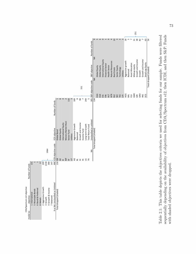
73mod

al ioc

objective

Num

ber of fu

nds

1International

131

5Mun

iciple Bon

ds1

6Bo

nd & Preferred

18Metals

172Aggressive Growth

209

3Growth

1218

4Growth & Income

390

7Ba

lanced

147

9 or NAUnclassified

or Unlisted

990ICDI objectiv

e code

ICDI objectiv

eNum

ber of fu

nds

150GB

Global Bon

d1

GE

Global Equ

ity8

IEInternational Equ

ity4

MF

Mon

ery Market M

uni

2SF

Sector Fun

d11

6UT

Utilities

3AG

Aggressive Growth

189

B LBa

lanced

8GI

Growth and

Income

98IN

Income Fund

7LG

Long

‐term Growth

244

TRTo

tal Return Fund

5

CDA/Spe

ctrum s12

objectiv

e

Total dropp

ed (shade

d)

551

1964

NA

Unclassified

or un

listed

305S&

P ob

jective code

S&P ob

jective

Num

ber of fu

nds

134

NA

NA

9EG

GGlobal Equ

ity5

EGX

Global Equ

ity6

EIG

International Equ

ity0

FIN

Financial Sector

1HLT

Health

Sector

9NTR

Natural Resou

rces

4RLE

Real Estate

10SEC

Sector Equ

ity3

TEC

Techno

log y

4UTI

Utilities

3AGG

Aggressive grow

th18

BAL

Balanced

5FLX

Asset Allocatio

n7

GMC

Midcap eq

uity

31GRI

Growth and

Income

38GRO

Growth

82ING

Growth and

Income

7SCG

Small‐cap

Equ

ity63 54

Total dropp

ed (shade

d)

Total dropp

ed (shade

d)

251

Tab

le2.

1:T

his

table

dep

icts

the

obje

ctiv

escr

iter

iaw

euse

dfo

rse

lect

ing

funds

for

our

sam

ple

.F

unds

wer

efilt

ered

sequen

tial

lydep

endin

gon

the

avai

labilit

yof

obje

ctiv

esfr

omC

DA

/Sp

ectr

um

s12,

then

ICD

I,an

dth

enS&

P.

Funds

wit

hsh

aded

obje

ctiv

esw

ere

dro

pp

ed.

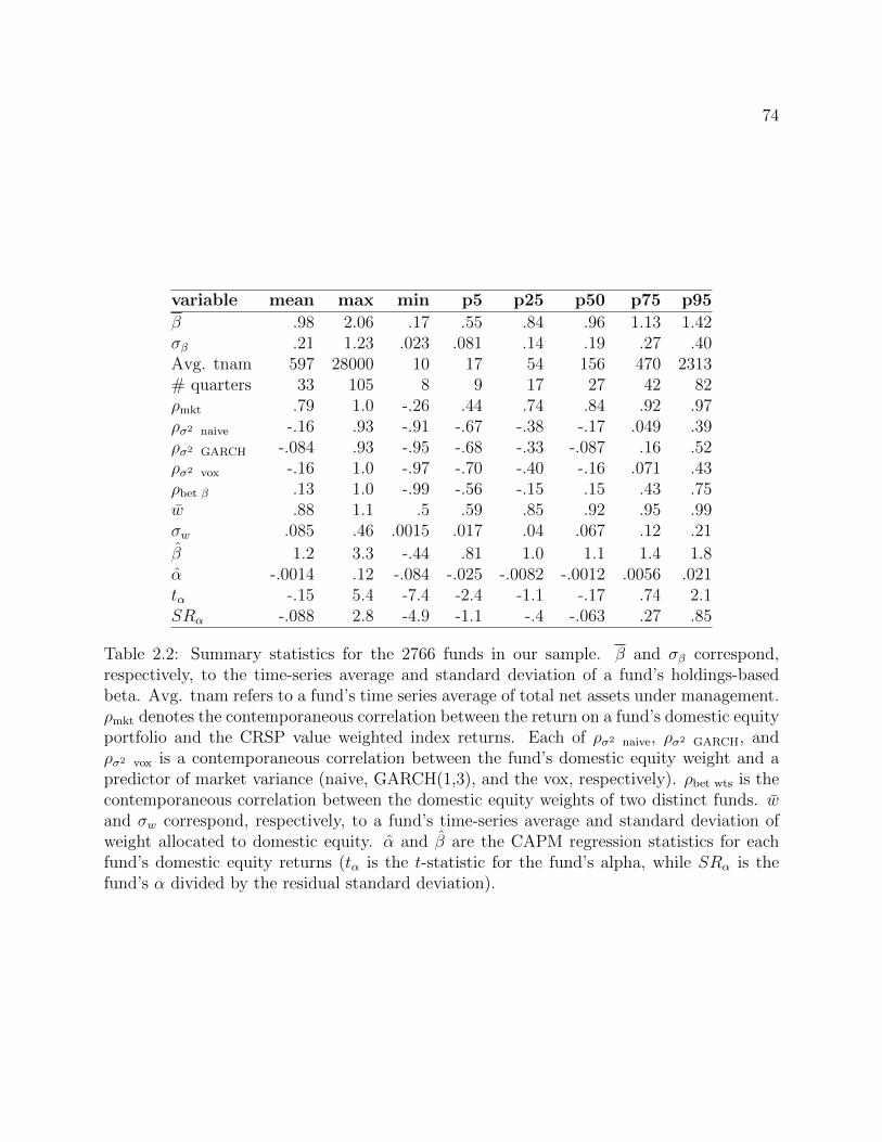
74

variable mean max min p5 p25 p50 p75 p95

β .98 2.06 .17 .55 .84 .96 1.13 1.42σβ .21 1.23 .023 .081 .14 .19 .27 .40Avg. tnam 597 28000 10 17 54 156 470 2313# quarters 33 105 8 9 17 27 42 82ρmkt .79 1.0 -.26 .44 .74 .84 .92 .97ρσ2 naive -.16 .93 -.91 -.67 -.38 -.17 .049 .39ρσ2 GARCH -.084 .93 -.95 -.68 -.33 -.087 .16 .52ρσ2 vox -.16 1.0 -.97 -.70 -.40 -.16 .071 .43ρbet β .13 1.0 -.99 -.56 -.15 .15 .43 .75w .88 1.1 .5 .59 .85 .92 .95 .99σw .085 .46 .0015 .017 .04 .067 .12 .21

β 1.2 3.3 -.44 .81 1.0 1.1 1.4 1.8α -.0014 .12 -.084 -.025 -.0082 -.0012 .0056 .021tα -.15 5.4 -7.4 -2.4 -1.1 -.17 .74 2.1SRα -.088 2.8 -4.9 -1.1 -.4 -.063 .27 .85

Table 2.2: Summary statistics for the 2766 funds in our sample. β and σβ correspond,respectively, to the time-series average and standard deviation of a fund’s holdings-basedbeta. Avg. tnam refers to a fund’s time series average of total net assets under management.ρmkt denotes the contemporaneous correlation between the return on a fund’s domestic equityportfolio and the CRSP value weighted index returns. Each of ρσ2 naive, ρσ2 GARCH, andρσ2 vox is a contemporaneous correlation between the fund’s domestic equity weight and apredictor of market variance (naive, GARCH(1,3), and the vox, respectively). ρbet wts is thecontemporaneous correlation between the domestic equity weights of two distinct funds. wand σw correspond, respectively, to a fund’s time-series average and standard deviation ofweight allocated to domestic equity. α and β are the CAPM regression statistics for eachfund’s domestic equity returns (tα is the t-statistic for the fund’s alpha, while SRα is thefund’s α divided by the residual standard deviation).

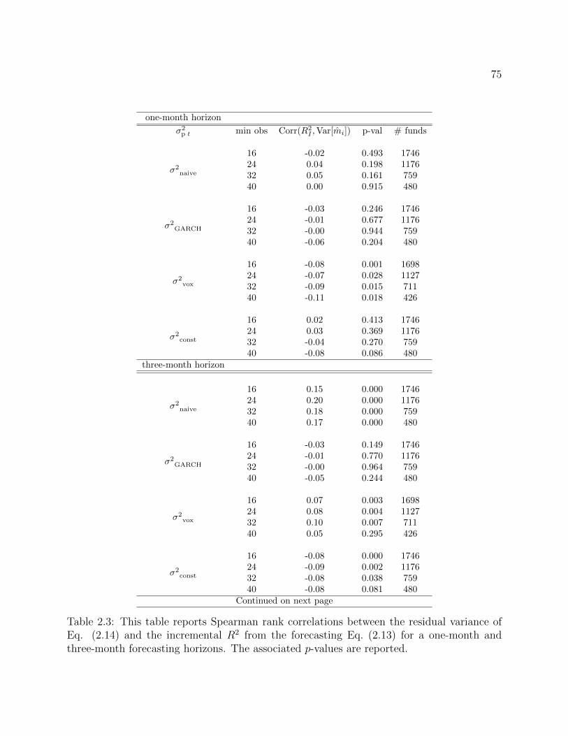
75

one-month horizon

σ2p t min obs Corr(R2

I ,Var[mi]) p-val # funds

σ2naive

16 -0.02 0.493 174624 0.04 0.198 117632 0.05 0.161 75940 0.00 0.915 480

σ2GARCH

16 -0.03 0.246 174624 -0.01 0.677 117632 -0.00 0.944 75940 -0.06 0.204 480

σ2vox

16 -0.08 0.001 169824 -0.07 0.028 112732 -0.09 0.015 71140 -0.11 0.018 426

σ2const

16 0.02 0.413 174624 0.03 0.369 117632 -0.04 0.270 75940 -0.08 0.086 480

three-month horizon

σ2naive

16 0.15 0.000 174624 0.20 0.000 117632 0.18 0.000 75940 0.17 0.000 480

σ2GARCH

16 -0.03 0.149 174624 -0.01 0.770 117632 -0.00 0.964 75940 -0.05 0.244 480

σ2vox

16 0.07 0.003 169824 0.08 0.004 112732 0.10 0.007 71140 0.05 0.295 426

σ2const

16 -0.08 0.000 174624 -0.09 0.002 117632 -0.08 0.038 75940 -0.08 0.081 480

Continued on next page

Table 2.3: This table reports Spearman rank correlations between the residual variance ofEq. (2.14) and the incremental R2 from the forecasting Eq. (2.13) for a one-month andthree-month forecasting horizons. The associated p-values are reported.

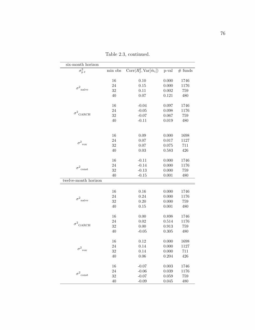
76

Table 2.3, continued.

six-month horizon

σ2p t min obs Corr(R2

I ,Var[mi]) p-val # funds

σ2naive

16 0.10 0.000 174624 0.15 0.000 117632 0.11 0.002 75940 0.07 0.121 480

σ2GARCH

16 -0.04 0.097 174624 -0.05 0.098 117632 -0.07 0.067 75940 -0.11 0.019 480

σ2vox

16 0.09 0.000 169824 0.07 0.017 112732 0.07 0.075 71140 0.03 0.583 426

σ2const

16 -0.11 0.000 174624 -0.14 0.000 117632 -0.13 0.000 75940 -0.15 0.001 480

twelve-month horizon

σ2naive

16 0.16 0.000 174624 0.24 0.000 117632 0.20 0.000 75940 0.15 0.001 480

σ2GARCH

16 0.00 0.898 174624 0.02 0.514 117632 0.00 0.913 75940 -0.05 0.305 480

σ2vox

16 0.12 0.000 169824 0.14 0.000 112732 0.14 0.000 71140 0.06 0.204 426

σ2const

16 -0.07 0.003 174624 -0.06 0.039 117632 -0.07 0.059 75940 -0.09 0.045 480

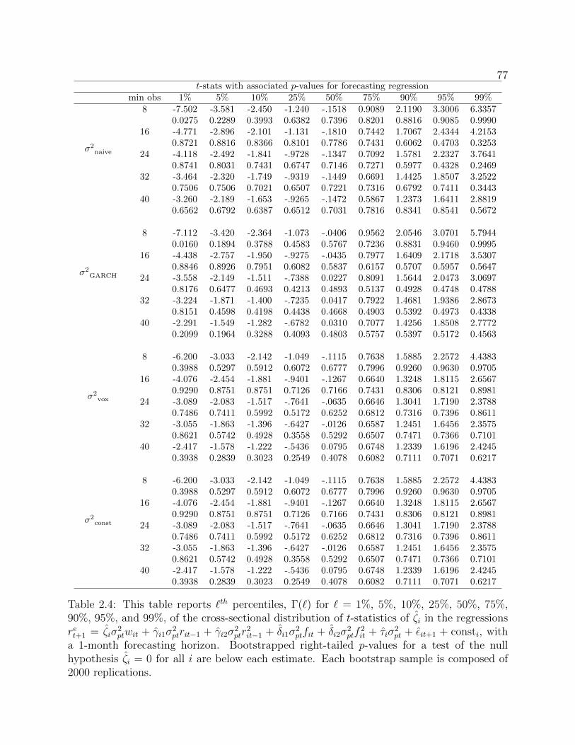
77t-stats with associated p-values for forecasting regression

min obs 1% 5% 10% 25% 50% 75% 90% 95% 99%

σ2naive

8 -7.502 -3.581 -2.450 -1.240 -.1518 0.9089 2.1190 3.3006 6.33570.0275 0.2289 0.3993 0.6382 0.7396 0.8201 0.8816 0.9085 0.9990

16 -4.771 -2.896 -2.101 -1.131 -.1810 0.7442 1.7067 2.4344 4.21530.8721 0.8816 0.8366 0.8101 0.7786 0.7431 0.6062 0.4703 0.3253

24 -4.118 -2.492 -1.841 -.9728 -.1347 0.7092 1.5781 2.2327 3.76410.8741 0.8031 0.7431 0.6747 0.7146 0.7271 0.5977 0.4328 0.2469

32 -3.464 -2.320 -1.749 -.9319 -.1449 0.6691 1.4425 1.8507 3.25220.7506 0.7506 0.7021 0.6507 0.7221 0.7316 0.6792 0.7411 0.3443

40 -3.260 -2.189 -1.653 -.9265 -.1472 0.5867 1.2373 1.6411 2.88190.6562 0.6792 0.6387 0.6512 0.7031 0.7816 0.8341 0.8541 0.5672

σ2GARCH

8 -7.112 -3.420 -2.364 -1.073 -.0406 0.9562 2.0546 3.0701 5.79440.0160 0.1894 0.3788 0.4583 0.5767 0.7236 0.8831 0.9460 0.9995

16 -4.438 -2.757 -1.950 -.9275 -.0435 0.7977 1.6409 2.1718 3.53070.8846 0.8926 0.7951 0.6082 0.5837 0.6157 0.5707 0.5957 0.5647

24 -3.558 -2.149 -1.511 -.7388 0.0227 0.8091 1.5644 2.0473 3.06970.8176 0.6477 0.4693 0.4213 0.4893 0.5137 0.4928 0.4748 0.4788

32 -3.224 -1.871 -1.400 -.7235 0.0417 0.7922 1.4681 1.9386 2.86730.8151 0.4598 0.4198 0.4438 0.4668 0.4903 0.5392 0.4973 0.4338

40 -2.291 -1.549 -1.282 -.6782 0.0310 0.7077 1.4256 1.8508 2.77720.2099 0.1964 0.3288 0.4093 0.4803 0.5757 0.5397 0.5172 0.4563

σ2vox

8 -6.200 -3.033 -2.142 -1.049 -.1115 0.7638 1.5885 2.2572 4.43830.3988 0.5297 0.5912 0.6072 0.6777 0.7996 0.9260 0.9630 0.9705

16 -4.076 -2.454 -1.881 -.9401 -.1267 0.6640 1.3248 1.8115 2.65670.9290 0.8751 0.8751 0.7126 0.7166 0.7431 0.8306 0.8121 0.8981

24 -3.089 -2.083 -1.517 -.7641 -.0635 0.6646 1.3041 1.7190 2.37880.7486 0.7411 0.5992 0.5172 0.6252 0.6812 0.7316 0.7396 0.8611

32 -3.055 -1.863 -1.396 -.6427 -.0126 0.6587 1.2451 1.6456 2.35750.8621 0.5742 0.4928 0.3558 0.5292 0.6507 0.7471 0.7366 0.7101

40 -2.417 -1.578 -1.222 -.5436 0.0795 0.6748 1.2339 1.6196 2.42450.3938 0.2839 0.3023 0.2549 0.4078 0.6082 0.7111 0.7071 0.6217

σ2const

8 -6.200 -3.033 -2.142 -1.049 -.1115 0.7638 1.5885 2.2572 4.43830.3988 0.5297 0.5912 0.6072 0.6777 0.7996 0.9260 0.9630 0.9705

16 -4.076 -2.454 -1.881 -.9401 -.1267 0.6640 1.3248 1.8115 2.65670.9290 0.8751 0.8751 0.7126 0.7166 0.7431 0.8306 0.8121 0.8981

24 -3.089 -2.083 -1.517 -.7641 -.0635 0.6646 1.3041 1.7190 2.37880.7486 0.7411 0.5992 0.5172 0.6252 0.6812 0.7316 0.7396 0.8611

32 -3.055 -1.863 -1.396 -.6427 -.0126 0.6587 1.2451 1.6456 2.35750.8621 0.5742 0.4928 0.3558 0.5292 0.6507 0.7471 0.7366 0.7101

40 -2.417 -1.578 -1.222 -.5436 0.0795 0.6748 1.2339 1.6196 2.42450.3938 0.2839 0.3023 0.2549 0.4078 0.6082 0.7111 0.7071 0.6217

Table 2.4: This table reports `th percentiles, Γ(`) for ` = 1%, 5%, 10%, 25%, 50%, 75%,90%, 95%, and 99%, of the cross-sectional distribution of t-statistics of ζi in the regressionsret+1 = ζiσ

2ptwit + γi1σ

2ptrit−1 + γi2σ

2ptr

2it−1 + δi1σ

2ptfit + δi2σ

2ptf

2it + τiσ

2pt + εit+1 + consti, with

a 1-month forecasting horizon. Bootstrapped right-tailed p-values for a test of the nullhypothesis ζi = 0 for all i are below each estimate. Each bootstrap sample is composed of2000 replications.

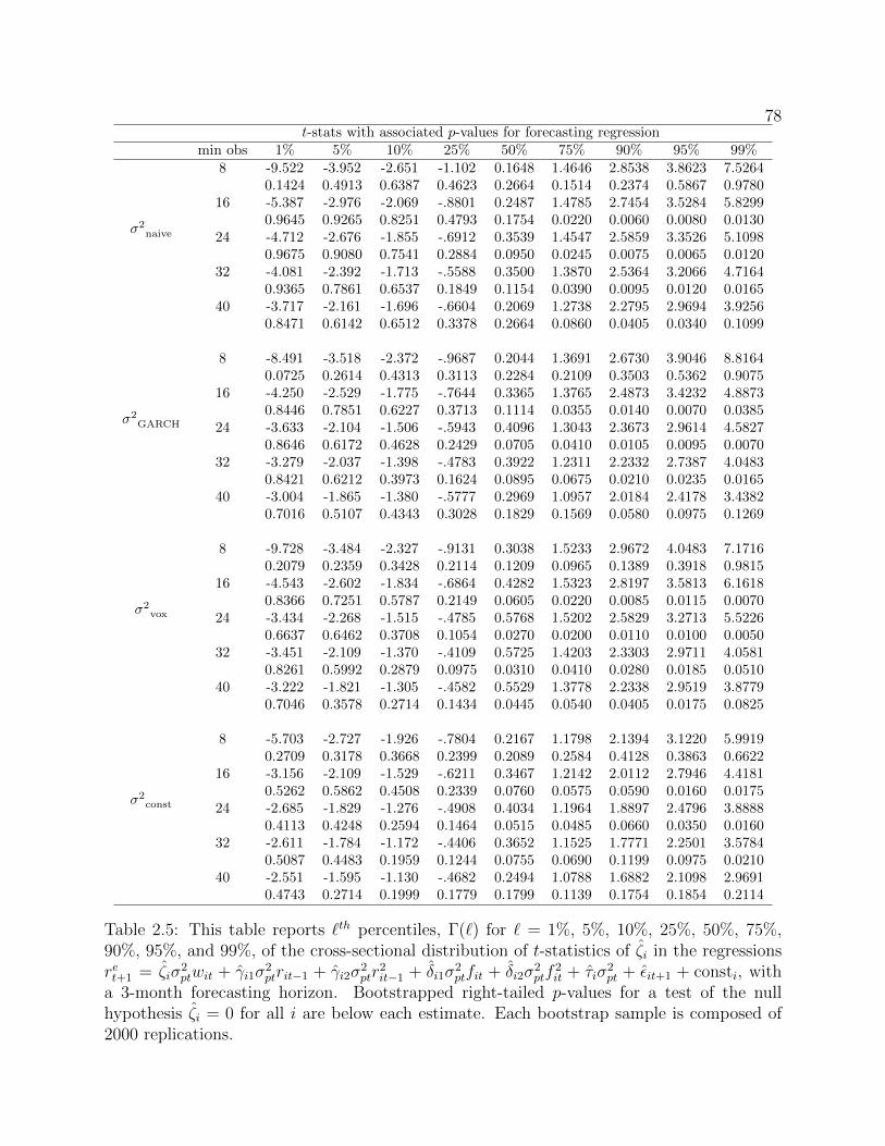
78t-stats with associated p-values for forecasting regression

min obs 1% 5% 10% 25% 50% 75% 90% 95% 99%

σ2naive

8 -9.522 -3.952 -2.651 -1.102 0.1648 1.4646 2.8538 3.8623 7.52640.1424 0.4913 0.6387 0.4623 0.2664 0.1514 0.2374 0.5867 0.9780

16 -5.387 -2.976 -2.069 -.8801 0.2487 1.4785 2.7454 3.5284 5.82990.9645 0.9265 0.8251 0.4793 0.1754 0.0220 0.0060 0.0080 0.0130

24 -4.712 -2.676 -1.855 -.6912 0.3539 1.4547 2.5859 3.3526 5.10980.9675 0.9080 0.7541 0.2884 0.0950 0.0245 0.0075 0.0065 0.0120

32 -4.081 -2.392 -1.713 -.5588 0.3500 1.3870 2.5364 3.2066 4.71640.9365 0.7861 0.6537 0.1849 0.1154 0.0390 0.0095 0.0120 0.0165

40 -3.717 -2.161 -1.696 -.6604 0.2069 1.2738 2.2795 2.9694 3.92560.8471 0.6142 0.6512 0.3378 0.2664 0.0860 0.0405 0.0340 0.1099

σ2GARCH

8 -8.491 -3.518 -2.372 -.9687 0.2044 1.3691 2.6730 3.9046 8.81640.0725 0.2614 0.4313 0.3113 0.2284 0.2109 0.3503 0.5362 0.9075

16 -4.250 -2.529 -1.775 -.7644 0.3365 1.3765 2.4873 3.4232 4.88730.8446 0.7851 0.6227 0.3713 0.1114 0.0355 0.0140 0.0070 0.0385

24 -3.633 -2.104 -1.506 -.5943 0.4096 1.3043 2.3673 2.9614 4.58270.8646 0.6172 0.4628 0.2429 0.0705 0.0410 0.0105 0.0095 0.0070

32 -3.279 -2.037 -1.398 -.4783 0.3922 1.2311 2.2332 2.7387 4.04830.8421 0.6212 0.3973 0.1624 0.0895 0.0675 0.0210 0.0235 0.0165

40 -3.004 -1.865 -1.380 -.5777 0.2969 1.0957 2.0184 2.4178 3.43820.7016 0.5107 0.4343 0.3028 0.1829 0.1569 0.0580 0.0975 0.1269

σ2vox

8 -9.728 -3.484 -2.327 -.9131 0.3038 1.5233 2.9672 4.0483 7.17160.2079 0.2359 0.3428 0.2114 0.1209 0.0965 0.1389 0.3918 0.9815

16 -4.543 -2.602 -1.834 -.6864 0.4282 1.5323 2.8197 3.5813 6.16180.8366 0.7251 0.5787 0.2149 0.0605 0.0220 0.0085 0.0115 0.0070

24 -3.434 -2.268 -1.515 -.4785 0.5768 1.5202 2.5829 3.2713 5.52260.6637 0.6462 0.3708 0.1054 0.0270 0.0200 0.0110 0.0100 0.0050

32 -3.451 -2.109 -1.370 -.4109 0.5725 1.4203 2.3303 2.9711 4.05810.8261 0.5992 0.2879 0.0975 0.0310 0.0410 0.0280 0.0185 0.0510

40 -3.222 -1.821 -1.305 -.4582 0.5529 1.3778 2.2338 2.9519 3.87790.7046 0.3578 0.2714 0.1434 0.0445 0.0540 0.0405 0.0175 0.0825

σ2const

8 -5.703 -2.727 -1.926 -.7804 0.2167 1.1798 2.1394 3.1220 5.99190.2709 0.3178 0.3668 0.2399 0.2089 0.2584 0.4128 0.3863 0.6622

16 -3.156 -2.109 -1.529 -.6211 0.3467 1.2142 2.0112 2.7946 4.41810.5262 0.5862 0.4508 0.2339 0.0760 0.0575 0.0590 0.0160 0.0175

24 -2.685 -1.829 -1.276 -.4908 0.4034 1.1964 1.8897 2.4796 3.88880.4113 0.4248 0.2594 0.1464 0.0515 0.0485 0.0660 0.0350 0.0160

32 -2.611 -1.784 -1.172 -.4406 0.3652 1.1525 1.7771 2.2501 3.57840.5087 0.4483 0.1959 0.1244 0.0755 0.0690 0.1199 0.0975 0.0210

40 -2.551 -1.595 -1.130 -.4682 0.2494 1.0788 1.6882 2.1098 2.96910.4743 0.2714 0.1999 0.1779 0.1799 0.1139 0.1754 0.1854 0.2114

Table 2.5: This table reports `th percentiles, Γ(`) for ` = 1%, 5%, 10%, 25%, 50%, 75%,90%, 95%, and 99%, of the cross-sectional distribution of t-statistics of ζi in the regressionsret+1 = ζiσ

2ptwit + γi1σ

2ptrit−1 + γi2σ

2ptr

2it−1 + δi1σ

2ptfit + δi2σ

2ptf

2it + τiσ

2pt + εit+1 + consti, with

a 3-month forecasting horizon. Bootstrapped right-tailed p-values for a test of the nullhypothesis ζi = 0 for all i are below each estimate. Each bootstrap sample is composed of2000 replications.

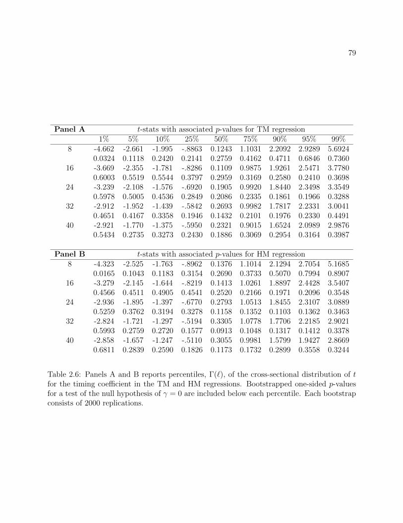
79

Panel A t-stats with associated p-values for TM regression1% 5% 10% 25% 50% 75% 90% 95% 99%

8 -4.662 -2.661 -1.995 -.8863 0.1243 1.1031 2.2092 2.9289 5.69240.0324 0.1118 0.2420 0.2141 0.2759 0.4162 0.4711 0.6846 0.7360

16 -3.669 -2.355 -1.781 -.8286 0.1109 0.9875 1.9261 2.5471 3.77800.6003 0.5519 0.5544 0.3797 0.2959 0.3169 0.2580 0.2410 0.3698

24 -3.239 -2.108 -1.576 -.6920 0.1905 0.9920 1.8440 2.3498 3.35490.5978 0.5005 0.4536 0.2849 0.2086 0.2335 0.1861 0.1966 0.3288

32 -2.912 -1.952 -1.439 -.5842 0.2693 0.9982 1.7817 2.2331 3.00410.4651 0.4167 0.3358 0.1946 0.1432 0.2101 0.1976 0.2330 0.4491

40 -2.921 -1.770 -1.375 -.5950 0.2321 0.9015 1.6524 2.0989 2.98760.5434 0.2735 0.3273 0.2430 0.1886 0.3069 0.2954 0.3164 0.3987

Panel B t-stats with associated p-values for HM regression8 -4.323 -2.525 -1.763 -.8962 0.1376 1.1014 2.1294 2.7054 5.1685

0.0165 0.1043 0.1183 0.3154 0.2690 0.3733 0.5070 0.7994 0.890716 -3.279 -2.145 -1.644 -.8219 0.1413 1.0261 1.8897 2.4428 3.5407

0.4566 0.4511 0.4905 0.4541 0.2520 0.2166 0.1971 0.2096 0.354824 -2.936 -1.895 -1.397 -.6770 0.2793 1.0513 1.8455 2.3107 3.0889

0.5259 0.3762 0.3194 0.3278 0.1158 0.1352 0.1103 0.1362 0.346332 -2.824 -1.721 -1.297 -.5194 0.3305 1.0778 1.7706 2.2185 2.9021

0.5993 0.2759 0.2720 0.1577 0.0913 0.1048 0.1317 0.1412 0.337840 -2.858 -1.657 -1.247 -.5110 0.3055 0.9981 1.5799 1.9427 2.8669

0.6811 0.2839 0.2590 0.1826 0.1173 0.1732 0.2899 0.3558 0.3244

Table 2.6: Panels A and B reports percentiles, Γ(`), of the cross-sectional distribution of tfor the timing coefficient in the TM and HM regressions. Bootstrapped one-sided p-valuesfor a test of the null hypothesis of γ = 0 are included below each percentile. Each bootstrapconsists of 2000 replications.

80

Mean 1% 5% 10% 25% 50% 75% 90% 95% 99%1-month horizon

γ -.21 -4.3 -2.4 -1.7 -.76 -.11 0.44 1.12 1.71 3.21p 0.83 0.91 0.92 0.90 0.83 0.72 0.63 0.56 0.51 0.54t -.19 -3.8 -2.3 -1.7 -.94 -.14 0.59 1.33 1.83 3.10p 0.73 0.83 0.74 0.64 0.67 0.67 0.76 0.74 0.72 0.583-month horizon

γ 0.08 -2.3 -1.1 -.70 -.24 0.12 0.45 0.79 1.09 2.00p 0.24 0.87 0.73 0.62 0.33 0.12 0.10 0.20 0.25 0.27t 0.27 -3.7 -2.1 -1.5 -.57 0.33 1.21 1.93 2.37 3.66p 0.16 0.80 0.63 0.47 0.21 0.12 0.07 0.09 0.14 0.206-month horizon

γ 0.10 -2.3 -1.1 -.69 -.20 0.15 0.45 0.81 1.07 2.04p 0.13 1.00 0.99 0.96 0.51 0.02 0.00 0.01 0.01 0.00t 0.40 -4.6 -2.5 -1.7 -.57 0.47 1.51 2.38 3.04 4.69p 0.08 0.99 0.94 0.76 0.24 0.05 0.00 0.00 0.00 0.0012-month horizon

γ 0.06 -1.8 -.89 -.57 -.18 0.10 0.34 0.59 0.82 1.53p 0.18 1.00 1.00 0.99 0.76 0.02 0.00 0.00 0.00 0.00t 0.39 -5.3 -3.1 -2.0 -.72 0.46 1.58 2.77 3.71 5.68p 0.08 1.00 1.00 0.96 0.44 0.06 0.00 0.00 0.00 0.00

Table 2.7: To generate this table we replicated the procedure used in Jiang, Yao, andYu (2007) (see their Table 3). The table reports percentiles (and the mean) of the cross-sectional distribution of γ and t for the holdings-based Trenor-Mazuy regression along withthe associated one-sided p-values given a null hypothesis that managers have no ability. Thebootstrap consists of 2000 replications.

81

+ - ++ - -FractionTM 0.5242 0.4758 0.0061 0.0042HM 0.5326 0.4674 0.0076 0.0061Mean timing coefficientTM 1.2298 -1.0387 1.2766 -2.1912HM 0.5819 -0.3903 0.4035 -0.6677

Table 2.8: The first two rows of report the fraction of estimated γi’s (timing coefficients asin Bollen and Busse, 2001) that are positive or negative (+,-) and significantly positive ornegative (++/- -). The second two rows report the conditional means of the γi’s, given thatthey are positive, negative, significantly positive, or significantly negative. Each bootstrapconsists of 2000 replications.

82

Bibliography

Admati, A. R., 1985, “A noisy rational expectations equilibrium for multi-asset securitiesmarkets,” Econometrica, 53(3), 629–657.

Admati, A. R., and P. Pfleiderer, 1986, “A monopolistic market for information,” Journalof Economic Theory, 39(2), 400–438.

, 1988, “Selling and trading on information in financial markets,” American EconomicReview, 78(2), 96–103.

Almazan, A., K. C. Brown, M. Carlson, and D. A. Chapman, 2004, “Why constrain yourmutual fund manager?,” Journal of Financial Economics, 73(2), 289–321.

An, M. Y., 1998, “Logconcavity versus logconvexity: A complete characterization,” Journalof Economic Theory, 80(2), 350–369.

Andrade, S., I. Babenko, and Y. Tserlukevich, 2006, “Market timing with cay,” Journal ofPortfolio Management, pp. 70–80.

Athey, S., 2002, “Monotone comparative statics under uncertainty,” Quarterly Journal ofEconomics, 117(1), 187–223.

Austin, K., 1987, “Finite and infinite systems,” The Mathematical Gazette, 71(456), 107–109.

Ausubel, L. M., 1990a, “Insider trading in a rational expectations economy,” AmericanEconomic Review, 80(5), 1022–1041.

, 1990b, “Partially-revealing rational expectations equilibrium in a competitive econ-omy,” Journal of Economic Theory, 50(1), 93–126.

Bagnoli, M., and T. Bergstrom, 2005, “Log-concave probability and its applications,” Eco-nomic Theory, 26(2), 445–469.

Bagnoli, M., S. Viswanathan, and C. Holden, 2001, “On the existence of linear equilibria inmodels of market making,” Mathematical Finance, 11(1), 1–31.

83

Banerjee, S., 2010, “Learning from prices and the dispersion in beliefs,” Working paper,Northwestern University.

Barlevy, G., and P. Veronesi, 2000, “Information acquisition in financial markets,” TheReview of Economic Studies, 67(1), 79–90.

, 2003, “Rational panics and stock market crashes,” Journal of Economic Theory,110(2), 234–263.

, 2008, “Information acquisition in financial markets: A correction,” Working paper.

Berk, J. B., and R. C. Green, 2004, “Mutual fund flows and performance in rational markets,”Journal of Political Economy, 112(6), 1269–1295.

Bernardo, A. E., and K. L. Judd, 2000, “Asset market equilibrium with general tastes,returns, and informational asymmetries,” Journal of Financial Markets, 3(1), 17–43.

Bhattacharya, U., and M. Spiegel, 1991, “Insiders, outsiders, and market breakdowns,”Review of Financial Studies, 4(2), 255–282.

Blackwell, D., 1951, “Comparison of experiments,” in Proceedings of the Second BerkeleySymposium on Mathematical Statistics and Probability, 1950, pp. 93–102, Berkeley andLos Angeles. University of California Press.

, 1953, “Equivalent comparisons of experiments,” Annals of Mathematical Statistics,24(2), 265–272.

Blume, L., D. Easley, and M. O’Hara, 1994, “Market statistics and technical analysis: Therole of volume,” Journal of Finance, 49(1), 153–181.

Bollen, N. P. B., and J. A. Busse, 2001, “On the timing ability of mutual fund managers,”Journal of Finance, 56(3), 1075–1094.

Bond, P., I. Goldstein, and E. S. Prescott, 2010, “Market-based corrective actions,” Reviewof Financial Studies, 23(2), 781–820.

Breen, W., L. R. Glosten, and R. Jagannathan, 1989, “Economic significance of predictablevariations in stock index returns,” Journal of Finance, 44(5), 1177–89.

Brown, D. P., and R. H. Jennings, 1989, “On technical analysis,” Review of Financial Studies,2(4), 527–551.

Brunnermeier, M. K., 2001, Asset Pricing under Asymmetric Information: Bubbles, Crashes,Technical Analysis, and Herding. Oxford University Press, New York.

84

Busse, J. A., 1999, “Volatility timing in mutual funds: Evidence from daily returns,” Reviewof Financial Studies, 12(5), 1009–41.

Campbell, J. Y., 2002, “Consumption-based asset pricing,” Harvard Institute of EconomicResearch Working Papers 1974, Harvard - Institute of Economic Research.

Campbell, J. Y., and R. J. Shiller, 1988a, “The dividend-price ratio and expectations offuture dividends and discount factors,” Review of Financial Studies, 1(3), 195–228.

Campbell, J. Y., and R. J. Shiller, 1988b, “Stock prices, earnings, and expected dividends,”Journal of Finance, 43(3), 661–76.

Chambers, C. P., and P. J. Healy, 2009, “Reversals of signal-posterior monotonicity for anybounded prior,” working paper.

Chamley, C., 2007, “Complementarities in information acquisition with short-term trades,”Theoretical Economics, 2(4), 441–467.

, 2008, “On “acquisition of information in financial markets”,” Review of EconomicStudies, 75(4), 1081–1084.

Chance, D. M., and M. L. Hemler, 2001, “The performance of professional market timers:Daily evidence from executed strategies,” Journal of Financial Economics, 62(2), 377–411.

Chang, E. C., and W. G. Lewellen, 1984, “Market timing and mutual fund investmentperformance,” Journal of Business, 57(1), 57–72.

Chen, J., H. Hong, and J. C. Stein, 2001, “Forecasting crashes: Trading volume, past returns,and conditional skewness in stock prices,” Journal of Financial Economics, 61(3), 345–381.

, 2002, “Breadth of ownership and stock returns,” Journal of Financial Economics,66(2-3), 171–205.

Cheng, H.-C., M. J. P. Magill, and W. J. Shafer, 1987, “Some results on comparative staticsunder uncertainty,” International Economic Review, 28(2), 493–507.

Chordia, T., 1996, “The structure of mutual fund charges,” Journal of Financial Economics,41(1), 3–39.

Cox, J. C., and H. E. Leland, 2000, “On dynamic investment strategies,” Journal of Eco-nomic Dynamics and Control, 24(11-12), 1859–1880.

Daniel, K., M. Grinblatt, S. Titman, and R. Wermers, 1997, “Measuring mutual fund per-formance with characteristic-based benchmarks,” Journal of Finance, 52(3), 1035–58.

85

Davis, M.H.A., ., and A. R. Norman, 1990, “Portfolio selection with transaction costs,”Mathematics of Operations Research, 15(4), 676–713.

DeMarzo, P., and C. Skiadas, 1998, “Aggregation, determinacy, and informational efficiencyfor a class of economies with asymmetric information,” Journal of Economic Theory, 80(1),123–152.

, 1999, “On the uniqueness of fully informative rational expectations equilibria,”Economic Theory, 13(1), 1–24.

Detemple, J. B., R. Garcia, and M. Rindisbacher, 2003, “A monte carlo method for optimalportfolios,” Journal of Finance, 58(1), 401–446.

Diamond, D. W., and R. E. Verrecchia, 1981, “Information aggregation in a noisy rationalexpectations economy,” Journal of Financial Economics, 9(3), 221–235.

Diether, K. B., C. J. Malloy, and A. Scherbina, 2002, “Differences of opinion and the crosssection of stock returns,” Journal of Finance, 57(5), 2113–2141.

Dimson, E., 1979, “Risk measurement when shares are subject to infrequent trading,” Jour-nal of Financial Economics, 7(2), 197–226.

Doukas, J. A., C. F. Kim, and C. Pantzalis, 2006, “Divergence of opinion and equity returns,”Journal of Financial and Quantitative Analysisin, 41(3), 573–606.

Dow, J., and R. Rahi, 2003, “Informed trading, investment, and welfare,” Journal of Busi-ness, 76(3), 439–454.

Eckbo, B. E., and D. C. Smith, 1998, “The conditional performance of insider trades,”Journal of Finance, 53(2), 467–498.

Edelen, R. M., 1999, “Investor flows and the assessed performance of open-end mutualfunds,” Journal of Financial Economics, 53(3), 439–466.

Eeckhoudt, L., and C. Gollier, 1995, “Demand for risky assets and the monotone probabilityratio order,” Journal of Risk and Uncertainty, 11(2), 113–122.

Fama, E. F., 1965, “The behavior of stock-market prices,” Journal of Business, 38(1), 34–105.

, 1991, “Efficient capital markets: II,” Journal of Finance, 46(5), 1575–1617.

Ferson, W. E., and R. W. Schadt, 1996, “Measuring fund strategy and performance inchanging economic conditions,” Journal of Finance, 51(2), 425–61.

86

Fishburn, P. C., and R. B. Porter, 1976, “Optimal portfolios with one safe and one risky asset:Effects of changes in rate of return and risk,” Management Science, 22(10), 1064–1073.

Fleming, J., C. Kirby, and B. Ostdiek, 2001, “The economic value of volatility timing,”Journal of Finance, 56(1), 329–352.

Foster, F. D., and S. Viswanathan, 1993, “The effect of public information and competitionon trading volume and price volatility,” Review of Financial Studies, 6(1), 23–56.

, 1996, “Strategic trading when agents forecast the forecasts of others,” Journal ofFinance, 51(4), 1437–1478.

French, K. R., G. W. Schwert, and R. F. Stambaugh, 1987, “Expected stock returns andvolatility,” Journal of Financial Economics, 19(1), 3–29.

Gallant, A. R., P. E. Rossi, and G. Tauchen, 1992, “Stock prices and volume,” The Reviewof Financial Studies, 5(2), 199–242.

Gallmeyer, M., B. Hollifield, and D. J. Seppi, 2005, “Demand discovery and asset pricing,”working paper.

Ganguli, J. V., and L. Yang, 2009, “Complementarities, multiplicity, and supply informa-tion,” Journal of the European Economic Association, 7(1), 90–115.

Garcıa, D., and G. Strobl, 2010, “Relative Wealth Concerns and Complementarities in In-formation Acquisition,” Review of Financial Studies, 24(1), 169–207.

Gennotte, G., and H. Leland, 1990, “Market liquidity, hedging, and crashes,” AmericanEconomic Review, 80(5), 999–1021.

Gervais, S., R. Kaniel, and D. H. Mingelgrin, 2001, “The high-volume return premium,”Journal of Finance, 56(3), 877–919.

Geweke, J., 2001, “A note on some limitations of CRRA utility,” Economics Letters, 71(3),341–345.

Gibbons, R. S., R. T. Holden, and M. L. Powell, 2010, “Rational-expectations equilibriumin intermediate good markets,” Working Paper 15783, NBER.

Glosten, L. R., R. Jagannathan, and D. E. Runkle, 1993, “On the relation between theexpected value and the volatility of the nominal excess return on stocks,” Journal ofFinance, 48(5), 1779–1801.

Goetzmann, W. N., J. Ingersoll, and Z. Ivkovic, 2000, “Monthly measurement of dailytimers,” Journal of Financial and Quantitative Analysis, 35(3), 257–290.

87

Goetzmann, W. N., and M. Massa, 2005, “Dispersion of opinion and stock returns,” Journalof Financial Markets, 8(3), 324–349.

Graham, J. R., and C. R. Harvey, 1996, “Market timing ability and volatility implied in in-vestment newsletters’ asset allocation recommendations,” Journal of Financial Economics,42(3), 397–421.

Grossman, S., 1976, “On the efficiency of competitive stock markets where trades havediverse information,” Journal of Finance, 31(2), 573–585.

Grossman, S. J., and J. E. Stiglitz, 1980, “On the impossibility of informationally efficientmarkets,” American Economic Review, 70(3), 393–408.

Grundy, B. D., and M. McNichols, 1989, “Trade and the revelation of information throughprices and direct disclosure,” Review of Financial Studies, 2(4), 495–526.

Hadar, J., and T. K. Seo, 1990, “The effects of shifts in a return distribution on optimalportfolios,” International Economic Review, 31(3), 721–736.

Hall, J. A., W. Brorsen, and S. H. Irwin, 1989, “The distribution of futures prices: Atest of the stable paretian and mixture of normals hypotheses,” Journal of Financial andQuantitative Analysis, 24(1), 105–116.

Hayek, F. A., 1945, “The use of knowledge in society,” American Economic Review, 35(4),519–530.

Hellwig, M. F., 1980, “On the aggregation of information in competitive markets,” Journalof Economic Theory, 22(3), 477–498.

Henriksson, R. D., 1984, “Market timing and mutual fund performance: An empirical inves-tigation,” Journal of Business, 57(1), 73–96.

Henriksson, R. D., and R. C. Merton, 1981, “On market timing and investment performance.Ii. Statistical procedures for evaluating forecasting skills,” Journal of Business, 54(4), 513–33.

Holden, C. W., and A. Subrahmanyam, 1992, “Long-lived private information and imperfectcompetition,” Journal of Finance, 47(1), 247–270.

Huang, J., C. Sialm, and H. Zhang, 2008, “Risk shifting and mutual fund performance,”Working paper, University of Texas at Austin.

Jagannathan, R., and R. A. Korajczyk, 1986, “Assessing the market timing performance ofmanaged portfolios,” Journal of Business, 59(2), 217–35.

88

Jewitt, I., 1987, “Risk aversion and the choice between risky prospects: The preservation ofcomparative statics results,” Review of Economic Studies, 54(1), 73–85.

, 1991, “Applications of likelihood ratio orderings in economics,” in Stochastic Ordersand Decision under Risk, vol. 19 of Lecture Notes-Monograph Series, pp. 174–189. Instituteof Mathematical Statistics.

Jiang, G. J., T. Yao, and T. Yu, 2007, “Do mutual funds time the market? Evidence fromportfolio holdings,” Journal of Financial Economics, 86, 724–758.

Kacperczyk, M., and A. Seru, 2007, “Fund manager use of public information: New evidenceon managerial skills,” Journal of Finance, 62(2), 485–528.

Kacperczyk, M., C. Sialm, and L. Zheng, 2005, “On the industry concentration of activelymanaged equity mutual funds,” Journal of Finance, 60(4), 1983–2011.

Kandel, S., and R. F. Stambaugh, 1996, “On the predictability of stock returns: An asset-allocation perspective,” Journal of Finance, 51(2), 385–424.

Karlin, S., 1968, Total Positivity, vol. 1. Stanford University Press, Stanford, CA, 1 edn.

Karpoff, J. M., 1987, “The relation between price changes and trading volume: A survey,”Journal of Financial and Quantitative Analysis, 22(1), 109–126.

Keim, D. B., and R. F. Stambaugh, 1986, “Predicting returns in the stock and bond mar-kets,” Journal of Financial Economics, 17(2), 357–390.

Kim, T. S., and E. Omberg, 1996, “Dynamic nonmyopic portfolio behavior,” Review ofFinancial Studies, 9(1), 141–161.

Kira, D., and W. T. Ziemba, 1980, “The demand for a risky asset,” Management Science,26(11), 1158–1165.

Kon, S. J., 1983, “The market-timing performance of mutual fund managers,” Journal ofBusiness, 56(3), 323–47.

, 1984, “Models of stock returns–a comparison,” Journal of Finance, 39(1), 147–165.

Koski, J. L., and J. Pontiff, 1999, “How are derivatives used? Evidence from the mutualfund industry,” Journal of Finance, 54(2), 791–816.

Kosowski, R., A. Timmermann, R. Wermers, and H. White, 2006, “Can mutual fund “stars”really pick stocks? New evidence from a bootstrap analysis,” Journal of Finance, 61(6),2551–2595.

89

Kothari, S., and J. Warner, 2001, “Evaluating mutual fund performance,” Journal of Fi-nance, 56(5), 1985–2010.

Kyle, A. S., 1985, “Continuous auctions and insider trading,” Econometrica, 53(6), 1315–1336.

, 1989, “Informed speculation with imperfect competition,” Review of EconomicStudies, 56(3), 317–355.

Landsberger, M., and I. Meilijson, 1990, “Demand for risky financial assets: A portfolioanalysis,” Journal of Economic Theory, 50(1), 204 – 213.

Lehmann, E. L., 1988, “Comparing location experiments,” Annals of Statistics, 16(2), 521–533.

Leland, H. E., 1980, “Who should buy portfolio insurance?,” Journal of Finance, 35(2),581–94.

Lettau, M., and S. Ludvigson, 2001, “Consumption, aggregate wealth and expected stockreturns,” Journal of Finance, 56, 815–849.

Ma, C., 1999, “On the posterior distribution of a location parameter from a strongly uni-modal distribution,” Statistics & Probability Letters, 42(1), 33–37.

Mandelbrot, B., 1963, “The variation of certain speculative prices,” Journal of Business,36(4), 394–419.

Manzano, C., and X. Vives, 2010, “Public and private learning from prices, strategic sub-stitutability and complementarity, and equilibrium multiplicity,” Working paper 3137,CESifo.

Milgrom, P. R., 1981, “Good news and bad news: Representation theorems and applica-tions,” The Bell Journal of Economics, 12(2), 380–391.

Milgrom, P. R., and R. J. Weber, 1982, “A theory of auctions and competitive bidding,”Econometrica, 50(5), 1089–1122.

Miller, E. M., 1977, “Risk, uncertainty, and divergence of opinion,” Journal of Finance,32(4), 1151–1168.

Peress, J., 2004, “Wealth, information acquisition, and portfolio choice,” Review of FinancialStudies, 17(3), 879–914.

Persico, N., 1996, “Information acquisition in affiliated decision problems,” Working paper1149, Northwestern University.

90

, 2000, “Information acquisition in auctions,” Econometrica, 68(1), 135–148.

Rochet, J.-C., and J.-L. Vila, 1994, “Insider trading without normality,” Review of EconomicStudies, 61(1), 131–152.

Romer, D., 1993, “Rational asset-price movements without news,” American Economic Re-view, 83(5), 1112–1130.

Schneider, J., 2009, “A rational expectations equilibrium with informative trading volume,”Journal of Finance, 64(6), 2783–2805.

Schwert, G. W., 1989, “Why does stock market volatility change over time?,” Journal ofFinance, 44(5), 1115–1153.

Shaked, M., and J. G. Shanthikumar, 2007, Stochastic Orders. Springer, New York.

Shumway, T., M. Szefler, and K. Yuan, 2009, “The information content of revealed beliefsin portfolio holdings,” Working paper, London School of Economics.

Simutin, M., 2009, “Excess Cash and Mutual Fund Performance,” Working paper, Universityof Toronto.

Taleb, N. N., 2007, The Black Swan. Random House, New York.

Taliaferro, R., 2009, “Market timing and crash timing: Predicting aggregate market returnswith mutual fund holdings,” Working paper, Harvard Business School.

Treynor, J. L., and K. Mazuy, 1966, “Can mutual finds outguess the market?,” HarvardBusiness Review, 44, 131–136.

Tucker, A. L., 1992, “A reexamination of finite- and infinite-variance distributions as modelsof daily stock returns,” Journal of Business & Economic Statistics, 10(1), 73–81.

Vanden, J. M., 2008, “Information quality and options,” Review of Financial Studies, 21(6),2635–2676.

Veldkamp, L. L., 2006a, “Information markets and the comovement of asset prices,” Reviewof Economic Studies, 73(3), 823–845.

, 2006b, “Media frenzies in markets for financial information,” American EconomicReview, 96(3), 577–601.

Wachter, J., 2002, “Portfolio and consumption decisions under mean-reverting returns: Anexact solution for complete markets,” Journal of Financial and Quantitative Analysis,37(1), 63–91.

91

Wermers, R., 2000, “Mutual fund performance: An empirical decomposition into stock-picking talent, style, transactions costs, and expenses,” Journal of Finance, 55(4), 1655–1703.

White, H., 1980, “A heteroskedasticity-consistent covariance matrix estimator and a directtest for heteroskedasticity,” Econometrica, 48(4), 817–38.

Whitelaw, R. F., 1994, “Time variations and covariations in the expectation and volatilityof stock market returns,” Journal of Finance, 49(2), 515–541.

, 1997, “Time-varying sharpe ratios and market timing,” New York University, SternSchool of Business, Working Paper Seires 98-074, New York University, Stern School ofBusiness.

Yan, X., 2006, “The determinants and implications of mutual fund cash holdings: Theoryand evidence,” Financial Management, 35(2), 67–91.

Yuan, K., 2005, “Asymmetric price movements and borrowing constraints: A rational expec-tations equilibrium model of crises, contagion, and confusion,” Journal of Finance, 60(1),379–411.

, 2006, “The price impact of borrowing and short-sale constraints,” Working paper,London School of Economics.

Documents

Essays on Asymmetric Information in Financial MarketsEssays on Asymmetric Information in Financial Markets by Bradyn Mitchel Breon-Drish A dissertation submitted in partial satisfaction