Estimating Asymmetric

Information Effects in Health Care Accounting for the Transactions

Costs

Yan Zheng Tomislav Vukina Xiaoyong Zheng

North Carolina State University Department of Agricultural and Resource Economics

Working Paper No. 17-005

September 2016

Estimating Asymmetric Information E�ects in Health

Care Accounting for the Transactions Costs

Yan Zheng, Tomislav Vukina∗and Xiaoyong Zheng

North Carolina State University

Abstract

We use a structural approach to separately estimate moral hazard and adverse selec-

tion e�ects in health care utilization using hospital invoices data. Our model explicitly

accounts for the heterogeneity in the transactions costs associated with hospital visits

which increase the individuals' total cost of health care and dampen the moral hazard

e�ect. A measure of moral hazard is derived as the di�erence between the observed

and the counterfactual health care consumption. In the population of patients with

non life-threatening diagnoses, our results indicate statistically signi�cant and econom-

ically meaningful moral hazard. We also test for the presence of adverse selection by

investigating whether patients with di�erent health status sort themselves into di�erent

health insurance plans. Adverse selection is con�rmed in the data because patients with

estimated worse health tend to buy the insurance coverage and patients with estimated

better health choose not to buy the insurance coverage.

JEL Classi�cation Numbers: C14, D82, I11

Keywords: Moral hazard, Adverse selection, Health insurance, Transaction Costs

Manuscript Word Count: 8,099

Table Count: 11

Figure Count: 2

Funding Sources: Research Assistantship from North Carolina State University

No potential con�icts of interest exist.

∗Correspondence: Department of Agricultural and Resource Economics, North Carolina State University,Raleigh, NC 27695. Telephone: 1-919-515-5864. Fax: 1-919-515-6268. E-mail: tom_vukina@ncsu.edu.

1

1 Introduction

The empirical literature dealing with the estimation of moral hazard and adverse selection

e�ects in health care utilization is quite large. For example, Manning et al. (1987) used a

randomized experiment and found that a catastrophic insurance plan reduces expenditures

31 percent relative to zero out-of-pocket price, indicating a large moral hazard e�ect. Using

the British Household Panel Survey, Olivella and Vera-Hernandez (2013) found that adverse

selection is present in the private health insurance market. Individuals who purchase private

health insurance (PHI) have a higher probability of both hospitalisation and visiting their

general practitioner than individuals who receive PHI as a fringe bene�t from employers.

Fewer studies succeeded in disentangling these two e�ects. For example, Wolfe and Goddeeris

(1991) estimated adverse selection as the e�ect of lag health status or lag health expenditure

on current insurance decisions in a longitudinal study of Medigap insurance. They found

a nontrivial decrease in moral hazard after taking into account the adverse selection. Liu,

Nestic and Vukina (2012) successfully disentangled moral hazard from adverse selection,

taking advantage of the unique features of health care system in Croatia. Using matching

estimators, they discovered favorable selection e�ect for patients in the 20-30 year cohort,

adverse selection for patients in older age cohorts and signi�cant moral hazard for all age

cohorts.

In this paper we rely on the structural approach to estimate the e�ects of moral hazard

and adverse selection using the hospital invoices data for non life-threatening diagnoses. The

data covers a four-month period in 2009 of all outpatient services provided to local patients

by a small regional hospital in Croatia. Croatia has a government controlled health care sys-

tem with a single payer insurance fund. The main contribution of this paper is seen in the

modeling and estimation approach which explicitly accounts for the heterogeneity in trans-

actions costs associated with hospital visit over and above the direct health care expenses.

By transactions costs we mean lost wages due to absenteeism from work, transportation

costs, hiring an escort or a babysitter, etc. We found that these transaction costs are large

2

and increase the individuals' total cost of health care signi�cantly.

Structural estimation of adverse selection and moral hazard has also been used in the

health insurance literature before. Earlier work was based on constructing health care de-

mand, using price elasticities as the measure of moral hazard, and the unexplained correlation

between insurance and health care demand as the measure of adverse selection. Cameron

et al. (1988) derived closed form demand functions for health insurance and health care for a

risk-averse consumer under uncertainty. Using data from 1977-1978 Australian Health Sur-

vey, they found a statistical dependence between error terms of health insurance and health

care demand equations which suggest the presence of adverse selection. They also found a

signi�cant price e�ect in health care consumption which identi�es the moral hazard as an

important determinant of the overall health care utilization. Cardon and Hendel (2001) in-

tegrated health insurance and health care demand using 1987 National Medical Expenditure

Survey data. Their objective was to estimate whether consumers' private information is an

important link between insurance and health care demand. They did not �nd any evidence of

adverse selection but found that the gap in expenditure between insured and uninsured can

be attributed to observable demographic di�erences and to price sensitivity. They concluded

that this price elasticity to coinsurance rate is an evidence of moral hazard. Vera-Hernandez

(2003) introduced a new measure of moral hazard based on the conditional correlation be-

tween contractible (treatment cost) and non-contractible (health shocks) variables. If this

correlation is zero, the relationship between the health shocks and treatment costs would

be deterministic and then there would be no moral hazard. Using RAND Health Insurance

Experiment data and simulated maximum likelihood estimator, the author uncovered the

structural model parameters. The results reject the nonexistence of moral hazard at 95%

con�dence level with about two-thirds of the variance of residual health shock explained

by the cost and one third left unexplained, a measure of moral hazard. Gardiol, Geo�ard

and Grandchamp (2005) developed a structural model of joint demand for health insurance

and health care. They took advantage of the design feature of the Swiss insurance system

3

where consumers choose their coverage from a menu of insurance plans ranked by the size of

their deductibles. They used insurance claims data and found evidence of both selection and

moral hazard e�ects. Their results indicate that 75% of the correlation between insurance

coverage and health care expenditures may be attributed to selection and 25% to ex post

moral hazard.

The most closely related to our paper is Bajari et al. (2014). They proposed a two-step

semiparametric estimation strategy to disentangle the adverse selection and moral hazard

e�ects in medical care. They used a unique claims data from a large self-insured employer

in the U.S. In the theoretical model, they introduced the latent health status parameter

into the utility function and used the GMM approach to estimate it. Moral hazard is then

estimated as the di�erence between health care consumption of people with the insurance

and their counterfactual consumption with no coverage. Adverse selection is examined by

comparing health status distributions of people in di�erent insurance plan groups. The fact

that people with worse latent health status sort themselves into insurance plan with higher

coverage is an evidence of adverse selection.

Our results show that, on average, the transactions costs amount to 42% of the incurred

medical expenses compared to the average out-of-pocket co-payment of only about 30%. We

also found a counterfactual evidence of moral hazard. If one takes away the insurance from

people with coverage, they would decrease their health care consumption by 32 HRK (8%).

If you give the insurance to people without coverage, they would increase their health con-

sumption by 27 HRK (9%). The presence of adverse selection was investigated by comparing

the empirical distributions of the estimated latent health status across groups of patients

with di�erent insurance types relying on the Kolmogorov-Smirnov test. The results indi-

cate the evidence of adverse selection in the sense that patients without the insurance are

relatively healthier than patients who bought the coverage.

4

2 Institutional Framework and Data Description

The main part of the data for this paper comes from Liu, Nestic and Vukina (2012). The

original data set consists of all invoices for all outpatient services from a regional hospital

in Croatia during the period from March 1 to June 30, 2009. The health care system

in Croatia is dominated by a single public health insurance fund: the Croatian Institute

for Health Insurance (HZZO). The HZZO o�ers two types of insurance: the compulsory

insurance and the supplemental insurance. The compulsory insurance's coverage is universal

and it is funded by a 15% payroll tax whereas the supplemental insurance can be either

bought or is extended automatically free of charge to certain categories of citizens. The

Croatian public health care system as provided by the HZZO is very similar to the Medicare

system in the U.S. The main di�erence is that the Croatian compulsory insurance insures

all citizens whereas Medicare provides limited public health insurance for the 65 years and

older citizens. The individuals covered by Medicare can choose to purchase Medigap to cover

the gaps in Medicare such as co-pays, deductibles and uncovered expenses (e.g. prescription

drugs, prolonged hospital stays, etc.). Medigap in the U.S. system plays the same role as the

supplemental insurance for Croatian citizens (for details see Liu, Nestic and Vukina, 2012).

The full coverage services a�orded by the compulsory insurance include: full health care

for children under the age of 18, health care of women related to pregnancy and child birth,

preventive and curative health care related to infectious diseases, mandatory vaccinations

and immunizations, hospital care for all chronic psychiatric patients, complete treatment of

all cancers, dialysis, organ transplants, emergency room interventions, house-calls and at-

home treatment of patients and prescription drugs from the HZZO basic list. All other health

services are subject to a system of co-payments (co-insurance)1. The insured are required

to pay a fraction of the full price of medical care, for example: laboratory, radiological

1It appears that Croatian system does not precisely distinguish co-payments from co-insurance in thesense of the �rst being the �at fee and the second being the percentage of the cost. The term actuallyused in English translation means "participation". However, the distinction is immaterial because prices ofmedical services (payments that providers receive from the HZZO) are �xed by HZZO and do not vary bythe provider and are also �xed for the period covered by our data.

5

and other diagnostics at the primary health care level (15.00 HRK), specialists' visits and

all out-patient services except physical therapy and rehabilitation (25.00 HRK), specialists'

diagnostics not at the primary care level (50 HRK), orthopedic and prosthetic devices (50

HRK), out-patient and at-home physical therapy and rehabilitation (25 HRK per day), in-

patient care (100 HRK per day), primary care including family physician, gynecologist and

dentist (15 HRK), etc. The largest out-of-pocket cost-share amount that a person can pay

amounts to 3,000.00 HRK per one invoice.2

Supplemental insurance is a voluntary insurance that can be acquired by a person 18 years

of age or older, having compulsory insurance, by signing a contract with HZZO. A person

having the supplemental insurance policy is entitled to full waiver of all medical expense co-

payments listed above. The premiums for supplemental insurance are determined as follows:

50.00 HRK per month for a retired person with the monthly pension of less than 5,108.00

HRK; 80.00 HRK per month for a retired person with pension higher than 5,108.00 HRK;

80.00 HRK per month for an active person with a monthly net income less than 5,108.00

HRK; 130.00 HRK per month for an active person with net income in excess of 5,108.00

HRK; 80.00 HRK per month for all family members and dependents.

An interesting feature of the supplemental insurance program is that certain categories

of people are exempt from paying the supplemental insurance; in other words, they are

entitled to it automatically for free. The list of exemptions is quite long. The top �ve largest

categories are poor people (59.17%), single pensioners (14.11%), people with 80% physical

disability (10.86%), blood donors (3.48%) and war veterans (2.96%). Therefore, with respect

to the supplemental insurance coverage we distinguish three categories of patients: those that

bought the insurance (Bought group), those that received the exact same insurance for free

(Free group) and those that do not have the insurance (No group). The analysis in the rest of

the paper involves only the comparison of health care consumption for diagnoses subject to

the system of co-payments, i.e. all other diagnoses covered in full by the universal compulsory

2Listed co-payments were valid for 2009. The exchange rate for the local currency, Croatian Kuna(HRK), as of June 20, 2009 was 1USD=5.19 HRK.

6

insurance program are ignored. Hence when we refer to patients with no insurance, we mean

patients with no supplemental insurance, i.e. those that are only covered by the universal

(compulsory) program.

The data set consists of 105,646 observations. Each observation re�ects the invoice for

one hospital visit. For the purpose of this estimation, patients who visited the hospital only

because of the illnesses that are fully covered by the compulsory insurance are excluded.

We also delete patients that are younger than 18 because there is no variation in the type

of insurance coverage for this group of people, i.e. they are all entitled to supplemental

insurance for free. The data contains the following set of variables: a numeric code for

the type of hospital service provided, compulsory health insurance number, supplemental

insurance number (if the patient has one), period covered by the supplemental insurance,

numeric code for categories entitled to supplemental insurance free of charge, eligibility

category for compulsory insurance (k1�employed, k2�farmers, k3�pensioners, k4�unemployed,

k5�living on social welfare, k6�self-employed and other), cost of hospital service, part of the

cost covered by compulsory insurance, part of cost covered by supplemental insurance, part

of cost covered by participation (co-payment), date of birth and sex of the patient. We

measure health care utilization using total cost per patient during the four-month period

covered by the data. The working data set consists of 70,851 invoices for 22,903 patients.

The summary statistics of the working data set is displayed in Table I. The No group has

smaller cost, younger population and larger percentage of men relative to the Bought and the

Free group. Each patient without the supplemental insurance (No group) paid on average

77.4 HRK in out-of-pocket co-payments during the 4-month period which amounts to less

than 1% of their income during the same time period. For patients in the other two groups,

the co-payment is zero because they are fully covered by the supplemental insurance.

In addition to invoice data set, we also use the Croatian Household Budget Survey

(CHBS) for 2009. The CHBS data set is used for the purpose of forecasting the income

variable for patients in the invoices data set. The dataset contains information on indi-

7

vidual's age, gender, eligibility category for compulsory insurance, supplemental insurance

status, household income, income per capita (household income divided by the number of

household members), individual income by source (employment, self-employment, unemploy-

ment bene�ts, pensions) and county of residence. The income variable used is de�ned as the

larger amount between the household income per capita and the sum of individual income

from all sources. There are a total of 8,269 individuals in the CHBS data set; 1,430 of them

are under the age of 18 and have been dropped. Among the remaining 6,839 observations,

305 are the residents of the county which coincides with the region from which our hospital

draws its patients.3 The summary statistics for the 6,839 observations sub-sample, broken

down by active versus retired population, is displayed in Table II. It is interesting to note

that there are people with zero income and also that the di�erence in mean income between

the active and retired citizens is not very large. Active people earn on average only HRK

2,593 (US$ 500) annually more than the retired people.

3 The model

The model relies on the assumption of a rational economic agent who maximizes his

utility function by choosing his optimal health care servicesm and consumption of composite

commodity c subject to a budget constraint. The utility function is additive in aggregate

consumption and health care, each in the constant relative risk aversion (CRRA) functional

form:

U(ci,mi; θi, γ) = (1− θi)c1−γ1i

1− γ1+ θi

m1−γ2i

1− γ2(1)

where γ1 and γ2 are risk-aversion coe�cients for aggregate and health care consumption. The

larger the coe�cients, the more risk averse the person with respect to variation in two types

of consumption. The utility also depends on latent health status parameter θ ∈ [0, 1], which

is known to the agent but unobservable by the insurance company. It can be interpreted as

3The actual name of the county is suppressed for con�dentiality reason because revealing the name ofthe county would automatically reveal the name of the hospital.

8

the importance weight an agent places on health care and aggregate consumption. In case

of bad health, θ is close to one, and the agent would gain relatively more utility from health

care consumption and less utility from other consumption.

A consumer's budget constraint requires that his expenditure on aggregate consumption

and health care must not be greater than his income minus the insurance premium:

ci +miβij ≤ yi − pj, (2)

where y is income, j denotes insurance status (no, bought, free), pj is the insurance premium

and βij is the co-payment rate which has two parts:

βij = αij + ϵi. (3)

In Equation (3), αij denotes the percentage of the cost that patients have to pay out of pocket

and it depends on the insurance coverage. If the patient has no supplemental insurance,

αij ∈ (0, 1); if the patient has the supplemental insurance either by buying it or being

entitled to it for free, αij = 0. Idiosyncratic cost ϵi > 0 represents the transactions costs

measured as a percentage of the cost of hospital services. It does not depend on the patient's

insurance status but varies with agent's income. The idea behind the speci�cation of the

cost factor βij is the fact that in addition to actual medical expenses which may or may not

be covered by the insurance, in order to see a doctor, the patient needs to invest time and

other resources, which is costly. These costs could be directly related to the lost income due

to absenteeism from gainful employment as well as a variety of other things such as the cost

of using own vehicle, a bus ticket, a taxi ride, a cost of hiring a baby-sitter or an escort, etc.

Notice that without ϵi, for patients with supplemental insurance, βij would be zero and the

model would predict the consumption of in�nite amount of health care.

The �rst order conditions for the maximization of utility (1) subject to budget constraint

9

(2) are as follows:

∂L∂ci

= (1− θi)c−γ1i − λ = 0,

∂L∂mi

= θim−γ2i − λβij = 0,

∂L∂λ

= yi − Pj − ci −miβij = 0.

The standard optimization result shows that the marginal rate of substitution between

aggregate consumption and health care consumption equals to the ratio of prices. However,

the price of health care that a consumer faces is only the co-payment portion αij of the actual

price plus the transactions costs related to the hospital visit ϵi.4 As a result, the relative

price of medical services to aggregate consumption is equal to βij and the MRS becomes:

MRS =θi

(1− θi)

cγ1imγ2

i

= αij + ϵi = βij (4)

Since a patient only needs to pay αij < 1 portion of the actual health care cost, the price

ratio between health care and aggregate consumption is biased towards favoring health care

and against general consumption. This �excess� of health care consumption is a standard

measure of moral hazard associated with insurance. However, the presence of ϵi in Equation

(4) changes the calculation because it makes the health care consumption less attractive,

thereby potentially mitigating the moral hazard e�ect. For some non-serious illness it could

actually make a di�erence between seeing and not seeing a doctor.

Since the utility function is strictly increasing, the budget constraint binds at the optimal

bundle. Therefore ci is determined by the equation ci = yi−pj−miβij = yi−pj−mi(αij+ϵi),

4Here, it is important to realize that even without the supplemental insurance, the patient will almostnever pay the full cost of the medical service, because some portion of it is always paid by the universal(compulsory) insurance.

10

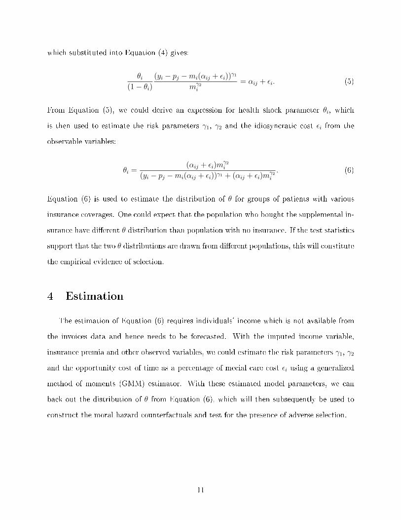
which substituted into Equation (4) gives:

θi(1− θi)

(yi − pj −mi(αij + ϵi))γ1

mγ2i

= αij + ϵi. (5)

From Equation (5), we could derive an expression for health shock parameter θi, which

is then used to estimate the risk parameters γ1, γ2 and the idiosyncratic cost ϵi from the

observable variables:

θi =(αij + ϵi)m

γ2i

(yi − pj −mi(αij + ϵi))γ1 + (αij + ϵi)mγ2i

. (6)

Equation (6) is used to estimate the distribution of θ for groups of patients with various

insurance coverages. One could expect that the population who bought the supplemental in-

surance have di�erent θ distribution than population with no insurance. If the test statistics

support that the two θ distributions are drawn from di�erent populations, this will constitute

the empirical evidence of selection.

4 Estimation

The estimation of Equation (6) requires individuals' income which is not available from

the invoices data and hence needs to be forecasted. With the imputed income variable,

insurance premia and other observed variables, we could estimate the risk parameters γ1, γ2

and the opportunity cost of time as a percentage of mecial care cost ϵi using a generalized

method of moments (GMM) estimator. With these estimated model parameters, we can

back out the distribution of θ from Equation (6), which will then subsequently be used to

construct the moral hazard counterfactuals and test for the presence of adverse selection.

11

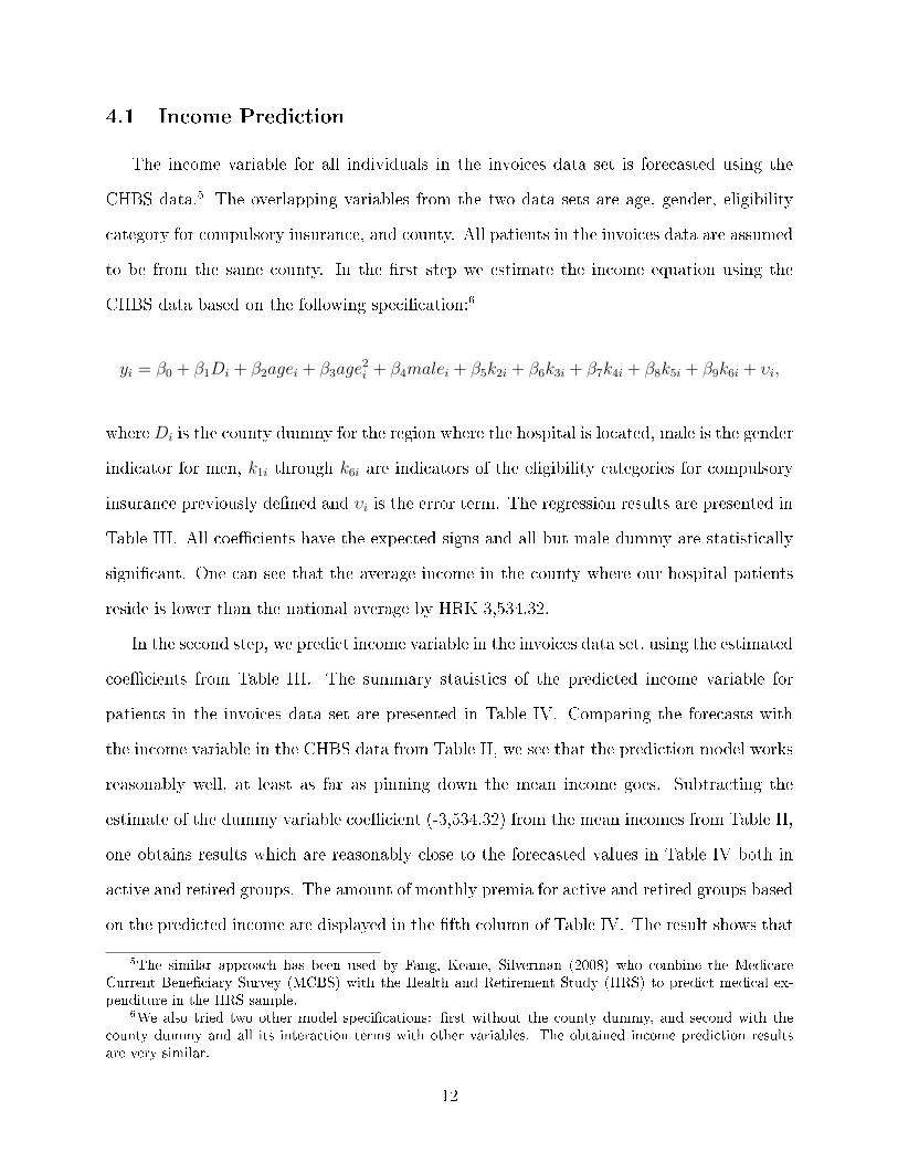
4.1 Income Prediction

The income variable for all individuals in the invoices data set is forecasted using the

CHBS data.5 The overlapping variables from the two data sets are age, gender, eligibility

category for compulsory insurance, and county. All patients in the invoices data are assumed

to be from the same county. In the �rst step we estimate the income equation using the

CHBS data based on the following speci�cation:6

yi = β0 + β1Di + β2agei + β3age2i + β4malei + β5k2i + β6k3i + β7k4i + β8k5i + β9k6i + υi,

where Di is the county dummy for the region where the hospital is located, male is the gender

indicator for men, k1i through k6i are indicators of the eligibility categories for compulsory

insurance previously de�ned and υi is the error term. The regression results are presented in

Table III. All coe�cients have the expected signs and all but male dummy are statistically

signi�cant. One can see that the average income in the county where our hospital patients

reside is lower than the national average by HRK 3,534.32.

In the second step, we predict income variable in the invoices data set, using the estimated

coe�cients from Table III. The summary statistics of the predicted income variable for

patients in the invoices data set are presented in Table IV. Comparing the forecasts with

the income variable in the CHBS data from Table II, we see that the prediction model works

reasonably well, at least as far as pinning down the mean income goes. Subtracting the

estimate of the dummy variable coe�cient (-3,534.32) from the mean incomes from Table II,

one obtains results which are reasonably close to the forecasted values in Table IV both in

active and retired groups. The amount of monthly premia for active and retired groups based

on the predicted income are displayed in the �fth column of Table IV. The result shows that

5The similar approach has been used by Fang, Keane, Silverman (2008) who combine the MedicareCurrent Bene�ciary Survey (MCBS) with the Health and Retirement Study (HRS) to predict medical ex-penditure in the HRS sample.

6We also tried two other model speci�cations: �rst without the county dummy, and second with thecounty dummy and all its interaction terms with other variables. The obtained income prediction resultsare very similar.

12

in both active and retired groups, the predicted income is always below the threshold (5,108

HRK/month) required for the insureds to pay higher premia. Hence, for all patients in the

invoices data, their income is low enough to make them eligible for the lower premium. This

result is somewhat unexpected, although certainly possible, in light of the fact that this

county's income is below the national average.

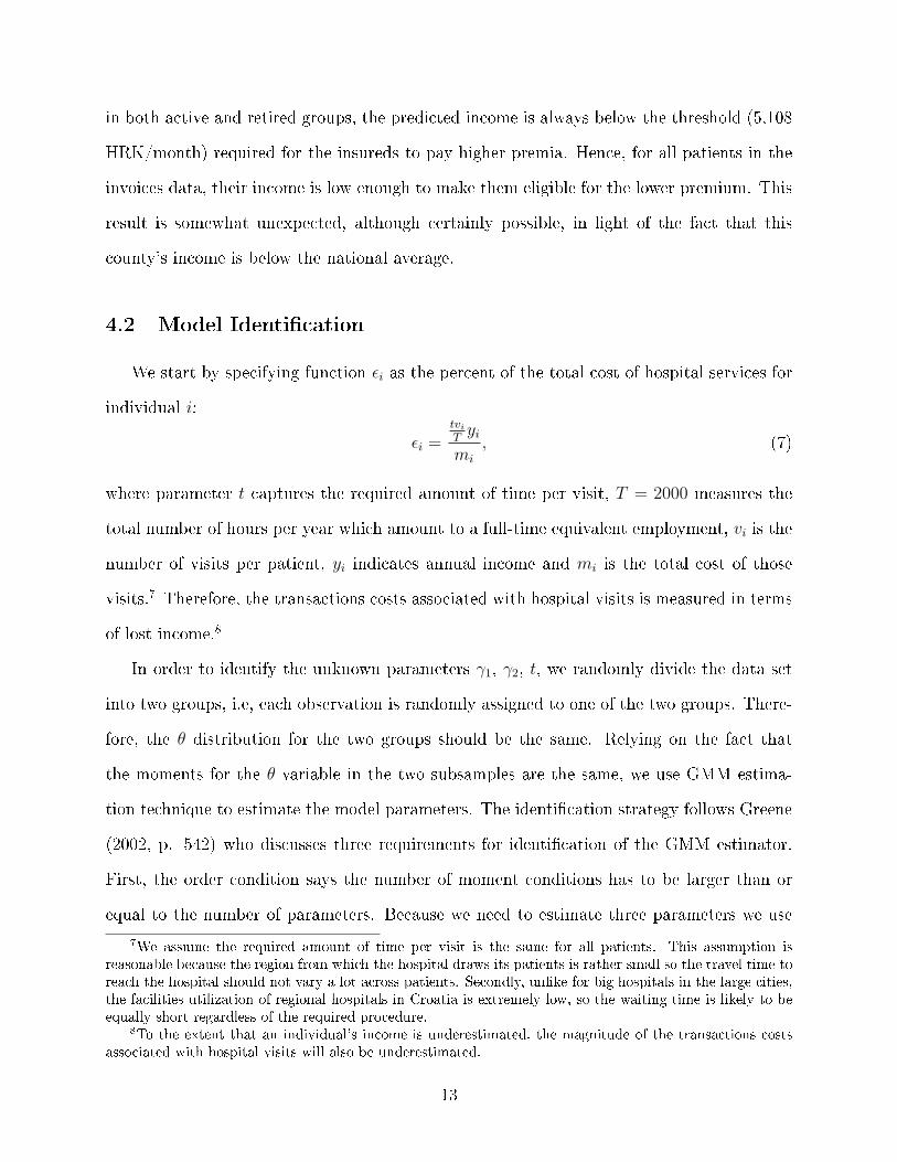
4.2 Model Identi�cation

We start by specifying function ϵi as the percent of the total cost of hospital services for

individual i:

ϵi =tviTyi

mi

, (7)

where parameter t captures the required amount of time per visit, T = 2000 measures the

total number of hours per year which amount to a full-time equivalent employment, vi is the

number of visits per patient, yi indicates annual income and mi is the total cost of those

visits.7 Therefore, the transactions costs associated with hospital visits is measured in terms

of lost income.8

In order to identify the unknown parameters γ1, γ2, t, we randomly divide the data set

into two groups, i.e, each observation is randomly assigned to one of the two groups. There-

fore, the θ distribution for the two groups should be the same. Relying on the fact that

the moments for the θ variable in the two subsamples are the same, we use GMM estima-

tion technique to estimate the model parameters. The identi�cation strategy follows Greene

(2002, p. 542) who discusses three requirements for identi�cation of the GMM estimator.

First, the order condition says the number of moment conditions has to be larger than or

equal to the number of parameters. Because we need to estimate three parameters we use

7We assume the required amount of time per visit is the same for all patients. This assumption isreasonable because the region from which the hospital draws its patients is rather small so the travel time toreach the hospital should not vary a lot across patients. Secondly, unlike for big hospitals in the large cities,the facilities utilization of regional hospitals in Croatia is extremely low, so the waiting time is likely to beequally short regardless of the required procedure.

8To the extent that an individual's income is underestimated, the magnitude of the transactions costsassociated with hospital visits will also be underestimated.

13

four moment conditions. Second, the rank condition says the gradient matrix of the moment

conditions must have a row rank that is equal to the number of parameters. Third, there

exists a unique vector of parameters that minimizes the objective function. However, as

Bajari et al. (2014) point out, in nonlinear parametric models, global identi�cation (second

and third identi�cation conditions) is generally di�cult to verify, hence these two identi�-

cation conditions have to be assumed. Intuitively, though, individual variations in latent

health status and in income and co-pay rate in the data lead to variations in medical ex-

penditure and general consumption. How the variations in medical expenditure and general

consumption are related to the variations in latent health status and income and co-pay rate

identify the risk aversion parameters as well as the parameter of the transactions cost func-

tion. Of course, functional form assumptions for the utility function and the transactions

cost function aid the identi�cation.

By setting the �rst four moments of health status distribution for two groups to be

equal, GMM optimal estimators γ̂1, γ̂2, t̂ minimize the sum of all moment conditions.9 Since

we nonparametrically match the shape of the distributions, we drop observations whose

medical cost are beyond 95% in the right tail of the expenditure distribution. The remaining

part of the sample has 21,758 patients.

The mean of the health status distribution for each of the two groups can be written as:

µθk(γ, t) =

Nk∑i=1

1

Nk

θi(γ, t), k = 1, 2; (8)

where Nk is the number of patients in group k; γ is a vector [γ1 γ2]. The variance of health

status distribution for each of the two groups can be written as:

V arθk(γ, t) =

Nk∑i=1

1

Nk

(θi(γ, t)− µθk(γ, t))2, k = 1, 2. (9)

9Bajari et al. (2014) used the same approach. However they have three years worth of data and theyassume that θ distribution does not change from one year to the next.

14

The skewness of health status distribution for each of the two groups can be written as:

Skθk(γ, t) =

Nk∑i=1

1

Nk

(θi(γ, t)− µθk(γ, t))3

varθk(γ, t)3/2

, k = 1, 2. (10)

and, �nally, the kurtosis of health status distribution for each of the two groups can be

written as:

Kuθk(γ, t) =

Nk∑i=1

1

Nk

(θi(γ, t)− µθk(γ, t))4

varθk(γ, t)2

− 3, k = 1, 2. (11)

To simplify the notation, we introduce vector w = (m, y, pj, αj), and de�ne moment condi-

tions as h(w, γ, t). In case of the mean we have one sample moment conditions:

h1(w, γ, t) = µθ̂1(γ, t)− µθ̂2

(γ, t) (12)

The sample moment conditions for variance, skewness, kurtosis are of the similar form.

Since two groups are drawn from same population, it follows that E[h(w, γ, t)] = 0. The

GMM estimators, γ̂1, γ̂2, t̂ minimize the sum of all 4 squared sample moment conditions,

which can be written compactly as the following objective function:

[γ̂1, γ̂2, t̂] = argmin4∑

k=1

h2k. (13)

We found the minimum of the objective function and hence the estimates γ̂1, γ̂2, t̂ by a grid

search over the parameter values γ̂1 ∈ [0, 10], γ̂2 ∈ [0, 10] and t̂ ∈ [0.5, 8]. The grid increment

for γ1, γ2 was set at 0.01 and the grid increment for t was set at 0.1. We restrict t to be

in the interval between half an hour and 8 hours because patients came to the hospital for

outpatient services only.

The main support for our identi�cation strategy comes from the law of large numbers.

With two random sub-samples from the same parent sample, the moments of the same

observable variables should be the same between the two sub-samples. The means for each

15

observable variable for both sub-samples are presented in Table V. We also test whether the

di�erences are statistically signi�cant and found that none of the di�erences are statistically

signi�cant which supports our identi�cation assumption.

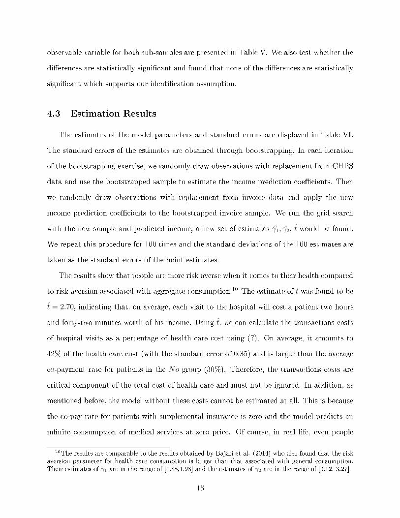
4.3 Estimation Results

The estimates of the model parameters and standard errors are displayed in Table VI.

The standard errors of the estimates are obtained through bootstrapping. In each iteration

of the bootstrapping exercise, we randomly draw observations with replacement from CHBS

data and use the bootstrapped sample to estimate the income prediction coe�cients. Then

we randomly draw observations with replacement from invoice data and apply the new

income prediction coe�cients to the bootstrapped invoice sample. We run the grid search

with the new sample and predicted income, a new set of estimates γ̂1, γ̂2, t̂ would be found.

We repeat this procedure for 100 times and the standard deviations of the 100 estimates are

taken as the standard errors of the point estimates.

The results show that people are more risk averse when it comes to their health compared

to risk aversion associated with aggregate consumption.10 The estimate of t was found to be

t̂ = 2.70, indicating that, on average, each visit to the hospital will cost a patient two hours

and forty-two minutes worth of his income. Using t̂, we can calculate the transactions costs

of hospital visits as a percentage of health care cost using (7). On average, it amounts to

42% of the health care cost (with the standard error of 0.35) and is larger than the average

co-payment rate for patients in the No group (30%). Therefore, the transactions costs are

critical component of the total cost of health care and must not be ignored. In addition, as

mentioned before, the model without these costs cannot be estimated at all. This is because

the co-pay rate for patients with supplemental insurance is zero and the model predicts an

in�nite consumption of medical services at zero price. Of course, in real life, even people

10The results are comparable to the results obtained by Bajari et al. (2014) who also found that the riskaversion parameter for health care consumption is larger than that associated with general consumption.Their estimates of γ1 are in the range of [1.88,1.98] and the estimates of γ2 are in the range of [3.12, 3.27].

16

with Cadillac health insurance do not consume in�nite quantities of health care, hence such

a model would be inconsistent with the observed behavior.

The estimated model parameters also allow us to compute compensated and uncompen-

sated demand elasticities for health care. From the �rst order condition (5), the implicit

di�erentiation yields

dmi

dβij

= −θi

(1−θi)

γ1(yi−pj−miβij)γ1−1

mγ2−1i

+ 1

θi(1−θi)

γ1(yi−pj−miβij)γ1−1

mγ2i

βij +θi

(1−θi)

γ2(yi−pj−miβij)γ1

mγ2+1i

.

and the uncompensated demand elasticity η = dmi

dβij

βij

mican be easily recovered. Also, implicit

di�erentiation of (5) yields

dmi

dyi=

θi(1−θi)

γ1(yi−pj−miβij)γ1−1

mγ2i

θi(1−θi)

γ1(yi−pj−miβij)γ1−1

mγ2i

βij +θi

(1−θi)

γ2(yi−pj−miβij)γ1

mγ2+1i

.

and by Slutsky decomposition, the compensated demand elasticity becomes ηC =dmc

i

dβij

βij

mci=

dmi

dβij

βij

mi+ βij

dmi

dyi.

The results are reported in Table VII. The mean uncompensated elasticity is -0.1245

and the mean compensated elasticity is -0.1216. These estimates are similar to the �ndings

in the previous literature. For example, Vera-Hernandez (2003) reported -0.108 for both

uncompensated and compensated elasticities when the co-pay rate is between 0% and 25%

and Manning et al. (1987) found uncompensated elasticity of -0.13.

Using estimated model parameters we can construct the distribution of θ based on Equa-

tion (6). In Figure 1 we provide a histogram plot (empirical pdf) of the distribution for

θ. The distribution has a long tail as we would expect in a typical health care expenditure

distribution. Most people are healthy and some are less so. We also regress θi on patients'

individual characteristics. Results are reported in Table VIII and, as expected, they indicate

that older people have worse health and high income people have better health. The gender

di�erence in health, as indicated by male dummy, is statistically insigni�cant.

17

5 Asymmetric Information E�ects

The use of terms moral hazard and adverse selection has its origins in the insurance

literature and then subsequently spread into contract theory and information economics.

The contract theory refers to moral hazard as an asymmetric information problem arising

when agent's (insured's) behavior is not observable by the principal (insurance company).

In the context of health insurance, however, moral hazard is often used in reference to the

price elasticity of demand for health care, conditional on underlying health status (Paully,

1968; Cutler and Zeckhauser, 2000; Einav et al. 2013). The approach that we use in the

treatment of moral hazard is conceptually in line with this mainstream health insurance

literature. In other words, our approach does not consider the potential impact of insurance

on the underlying health θ. When it comes to adverse selection, both strains of the literature

refers to the same problem which appears when the agent (insured) holds private information

before the relationship with the principal begins (i.e., before the insurance contract is signed).

In this case, the principal can possibly verify the agent's behavior, but the optimal decision

or its cost depends on agent's type (for example her health status) of which the agent is the

only informed party.

5.1 Moral Hazard

To estimate the magnitude of moral hazard, we run two counterfactual experiments.

First, we take away the supplemental insurance from people in Bought group and calculate

their counterfactual health expenses in the absence of supplemental insurance. In the �rst

experiment, a patient has to pay the part of cost that was originally covered by supplemental

insurance out of pocket. This means that their out of pocket expenses as a percentage of

the health care cost which was only ϵi (the price ratio is ϵi), in the absence of supplemental

insurance, increases to (αij + ϵi). The consumer is also provided with a lump sum income

transfer equal to the amount originally covered by supplemental insurance to ensure the

18

original consumption bundle (c1,m1) is a�ordable. This removes the income e�ect from the

price change in health care relative to other goods and allows us to focus on the substitution

e�ect.11

Next, we need to explain how to calculate m2 for each individual in Bought group.

Denote the lump sum income transfer as Ti = αijm1i, where αij is the portion covered by

supplemental insurance (observed in the data). In the counterfactual scenario, patient i pays

the amount αijm2i out of pocket and the budget constraint becomes:

c2i +m2i(αij + ϵi) ≤ yi − pj + Ti (14)

Next, we need to solve the optimization problem. With the binding budget constraint, c2

can be expressed as c2i = yi − pj − m2i(αij + ϵi) + Ti and the agent's utility function that

needs to be maximized becomes:

U(m2i, pj, yi; θi, ϵi, γ) = (1− θi)(yi − pj −m2i(αij + ϵi) + Ti)

1−γ1

1− γ1+ θi

m1−γ22i

1− γ2. (15)

The �rst order conditions set the marginal rate of substitution between aggregate consump-

tion and health care equal to the price ratio. In the absence of supplemental insurance, a

consumer pays his share (αij + ϵi) out of pocket. The price ratio is then equal to (αij + ϵi)

and the marginal rate of substitution becomes:

MRS =θi

(1− θi)

(yi − pj −m2i(αij + ϵi) + Ti)γ1

mγ22i

= αij + ϵi. (16)

Since the health status parameter θi, risk parameters γ1, γ2, and the idiosyncratic cost ϵi

11The patients in the Free group are not used in this experiment because of the data coding problem. Inmany instances the entire cost of the visit has been charged to the compulsory insurance and zero to thesupplemental insurance. Hence, when losing the insurance the patient in the Free group is now required topay certain percentage of the cost as a co-payment, but any percent of zero is still zero. Notice, however,that this data coding problem does not a�ect the estimation for γ̂1, γ̂2, t̂ because for estimation purposeswe only need total cost per patient rather than a part covered by compulsory and a part covered by thesupplemental insurance.

19

are all unchanged, we can use their estimates obtained in Section 4.2 and solve for the only

unknown variable, m2i using Equation (16). The di�erence between the observed health

care consumption m1i and the counterfactual health care consumption m2i is caused by the

change in price ratio and represents a measure of moral hazard. The standard errors of

estimates for moral hazard are obtained through bootstrapping. We calculate estimate of

moral hazard with the updated γ̂1, γ̂2, t̂ in each iteration of the bootstrapped invoice samples.

Standard deviations of the 100 estimates are taken as standard errors of the point estimates.

For each patient, the moral hazard is measured by the di�erence between the counter-

factual and the original health care expenditure, ∆mi = m2i −m1i or as a percent change

in the original health care expenditure, %∆mi =m2i−m1i

m1i. The averages across all patients

in di�erent groups are reported in Table IX. The results show that people in Bought group

would spend 31.86 HRK or 8.3% less on health care if we take away their supplemental

insurance. Because our data is limited only to the observations of people who came to the

hospital and sought medical help, the estimates of moral hazard would normally be impacted

by the "users only" data problem. However, in this particular counterfactual experiment,

the estimate of moral hazard is unbiased because taking away insurance from non-users do

not change their behavior. People who did not visit the doctor when they had insurance,

surely would not visit the doctor when they don't have insurance.

Using this counterfactual experiment it is also meaningful to sum up all individual mea-

sures of moral hazard to come up with the aggregate measure of moral hazard for the

county/hospital as a whole. As seen from Table IX, the aggregate 4-months hospital level

reduction in health care consumption due to elimination of moral hazard amounts to 375

thousand HRK (about 72 thousand dollars) or 9.09%.

In the second counterfactual scenario we give supplemental insurance to the patients

in the No group and calculate their counterfactual health expenses assuming they have

supplemental insurance. In this scenario the patients only need to pay the share ϵimi out of

pocket. There is also an income transfer, Ti = −αijm1i, which is negative because it takes

20

away part of the income which was originally spent on health care consumption. Then, the

budget constraint becomes:

c2i +m2iϵi ≤ yi − pj + Ti. (17)

Substituting the binding budget constraint for c2i in the utility function yields:

U(m2i, pj, yi; θi, ϵi, γ) = (1− θi)(yi − pj −m2iϵi + Ti)

1−γ1

1− γ1+ θi

m1−γ22i

1− γ2. (18)

Finding maximum would reveal the optimal allocation bundle achieved at the point where

the marginal rate of substitution between aggregate consumption and health care equals the

price ratio ϵi and the marginal rate of substitution will once again become:

MRS =θi

(1− θi)

(yi − pj −m2iϵi + Ti)γ1

mγ22i

= ϵi. (19)

Same as before, for each observation, the only unknown variable is m2i which could be solved

for each patient using Equation (19). We expect the counterfactual health care m2i to be

greater than the observed m1i. Thus, the di�erence between the counterfactual m2i and the

observed m1i is the amount a patient would over-consume as a result of price distortion due

to the supplemental insurance and it represents an alternative measure of moral hazard.

As seen from Table IX, people in the No group would have spent 27.25 HRK more

on health care once they were provided with the supplemental insurance. This measure

of moral hazard su�ers from the "users only" data problem because in this counterfactual

experiment we cannot give the insurance to the people in the No group who never showed in

the hospital (non-users) because we don't know who they are and how many of them there

are. Therefore this measure surely understates the true magnitude of moral hazard in the

general population.

21

5.2 Adverse Selection

In the presence of adverse selection, the patients with no supplemental insurance (No) and

the patients who bought the supplemental insurance (Bought) should have di�erent health

status distributions. We �rst estimate the relationship between patients' characteristics and

insurance status using logistic regression. The outcome variable is the insurance: for the

Bought group Yi = 1 and for the No group Yi = 0. The results give the marginal e�ect of

the regressors on the probability of purchasing the insurance. The �rst speci�cation includes

only demographic covariates: age, gender and income. We expect the marginal e�ects of

age and income to be positive and gender (male) to be negative, meaning that older, richer

and female patients are more likely to buy the supplemental insurance relative to their

counterparts. The second logit model includes demographic covariates and estimated health

status θ̂. A larger value of θ denotes relatively worse underlying health status. We expect

that the estimated health status θ̂ has a positive marginal e�ect because patients who bought

the supplemental insurance did so in anticipation of frequently using it.

In addition to logistic regression, the presence of selection can be also tested by comparing

estimated θ distributions between insurance plans. In the presence of adverse selection, we

would expect distribution of the latent health status be signi�cantly di�erent between plans,

with higher θ patients choosing more insurance and lower θ patients choosing less insurance.

The absence of adverse selection would be indicated by the health status distributions being

identical between insurance plans. We perform the Kolmogorov-Smirnov test for the equality

of θ distributions between insurance plans. The null hypothesis is that θ distributions for two

plans come from the same population. We also use Kolmogorov-Smirnov test to determine

whether the cdf of θ distribution for one plan is stochastically dominating that for the other.

The plan with a dominating cdf has more consumers with lower value of θ (healthier). One

would expect that in the presence of adverse selection, the patients in the No group should

be comparatively healthier (lower value of θ) and the cdf of θ distribution in the No group

should stochastically dominate the cdf of the θ distribution for the Bought group.

22

Finally, one cannot rule out the presence of favorable selection either. This is because

people can buy more or less insurance for reasons which are not only related to their risk-

aversion and health status but could be additionally impacted by other sources of unobserved

heterogeneity.12 In the presence of favorable selection, the cdf of θ distribution of the Bought

group should stochastically dominate the cdf of the No group.

The results for logistic regression are displayed in Table X. It reports the marginal e�ects

of consumer characteristics and health status on the insurance plan choice. The �rst model

includes only demographic characteristics, whereas the second model includes demographic

characteristics and the estimate of the latent health status variable θ̂. Most results in Model

1 are as expected. The marginal e�ect of age is positive and the marginal e�ect of gender

(male) is negative. It means that older and female patients are more likely to purchase

the supplemental insurance than their counterparts. An unexpected result is that income

has negative marginal e�ect which means that richer individuals are less likely to buy the

supplemental insurance than the poor ones. This result can be interpreted by realizing that

rich people can self-insure themselves against adverse e�ects of illness. This is especially

true in Croatia where the compulsory insurance provides a very generous safety net for all

citizens whereas the supplemental insurance covers expenses which are unlikely to cause a

serious �nancial hardship for more a�uent citizens. The results in Model 2 which includes

the estimated latent health status do not reverse any of the results from Model 1. As far

as the health status is considered, it has positive e�ect on Bought group. With larger value

of θ indicating worse health, this result suggests that people without insurance tend to be

relatively healthier and people who decided to buy the insurance tend to be in worse health.

Next, we test the adverse selection e�ect by comparing θ distributions. The two-sided

and one-sided test results are reported in Table XI. The two-sided test results show that

patients in two groups have di�erent health status distributions and the results are statisti-

12Fang, Keane and Silverman (2008) found evidence of advantageous selection in the Medigap insurancemarket and suggested that the sources of this advantageous selection include the insureds' income, education,longevity expectations, �nancial planning horizons and especially the cognitive ability.

23

cally signi�cant at 1%. Finally, we test whether the cdf of the θ distribution for No group is

dominating that of Bought group. The group with the dominating cdf of the θ distribution

has more people on the lower end of the distribution, which means it has larger percentage of

healthier people. The null hypotheses that the distributions are the same are tested against

the alternative that the cdf of the θ distribution for No is greater than the cdf of the θ distri-

bution for Bought. The one-sided test results show that the cdf of the θ distribution for the

No group is signi�cantly dominating that of Bought group. It means healthier people self-

selected themselves into No group, while people with comparatively worse health self-select

themselves into the Bought group. These results provide strong, statistically signi�cant,

evidence of adverse selection.

The enlarged versions of cdf distributions of θ for two groups are plotted in Figure 2.

The graph clearly shows that the cdf of θ distribution for Bought group is stochastically

dominated by the cdf of the θ distribution for No group, indicating that people in No group

are generally healthier than people in the Bought group.

6 Conclusion

This paper uses a structural approach to estimate clean moral hazard e�ect in health

insurance, net of possible in�uences of adverse selection. We found positive and economically

meaningful e�ect of moral hazard and also a statistically signi�cant e�ect of adverse selection

in the population of hospital patients.

An important methodological contribution of our paper is to take into account individual

patients' the transactions costs associated with medical care consumption. To the best of

our knowledge this is the �rst attempt in the literature to incorporate such cost into a

structural estimation of health care demand. We argue that this cost does not depend on

the providers' price nor the insurance type but depends on agent's income. The idea behind

this speci�cation is the fact that in addition to actual medical expenses which may or may not

24

be covered by the insurance, di�erent people could have di�erent transaction costs associated

with visiting a hospital or a doctor, which for certain minor illnesses could deter the health

care consumption thus mitigating the moral hazard problem.

The generalization of the obtained results for the purposes of country level and interna-

tional comparisons is somewhat hampered by the fact that hospital invoices data is comprised

of users only, i.e., we don't have data for insured and uninsured citizens with zero medical

consumption in the given period. As it turns out, the obtained structural model parameter

estimates (γ̂1, γ̂2, t̂) are still consistent because the structural model is assumed for users and

non-users alike and equation (6) used to estimate θi for individuals with di�erent insurance

coverage is also valid for both users and nonusers. However, two important consequences of

the users only data still remain.

First, the two counterfactual moral hazard scenarios are markedly di�erent. The scenario

where we take away the supplemental insurance from the insured users and simulate their

counterfactual health expenses in the absence of this insurance gives the correct estimate of

the moral hazard e�ect at the aggregate (hospital) level. This is true in light of the fact that

the insured nonusers are not going to be impacted by taking away the insurance from them

because if they did not go to the hospital when they had insurance, they surely will not go

when they don't have the insurance. The second scenario where we give the insurance to

uninsured users su�ers from the fact that uninsured users group does not encompass people

who did not seek medical attention precisely because they lacked the insurance. Therefore,

giving the insurance to uninsured citizens would impact not only users but potentially also

nonusers who do not appear in our data. Hence the second scenario is surely going to

under-estimate the magnitude of the moral hazard. The di�erence between two scenarios is

attributable to the users only data problem.

Second, the tests for adverse selection are also impacted by the users only data problem

because these tests should be based on the distribution of the unobserved health status θ

for the entire population whereas ours are based on users only. Our estimates of θi overstate

25

the true health status in the overall population, making it worse than it really is. There are

two reasons for this phenomenon, both pooling in the same direction. First, among those

insured, it is reasonable to assume that most of those that need medical help will actually

demand it and hence will show up as users. Only those, with relatively minor illnesses and

high transactions costs associated with hospital visits will not seek medical attention when

they need it and will not show up as users. The rest of the insured population simply did

not need medical attention and never showed up in the hospital. Hence, the actual health

status of the entire Bought group is likely to be better (lower θ) than the actual patients

(users only) based estimates. Next, the users only based estimates of θi for the No group

is also likely to overstate the true health status of this entire group because it is possible

that some people who do not have the insurance did not show up in the hospital to seek

medical attention precisely because they did not have the insurance. The unobserved health

status of those individuals (nonusers) is likely to be better than those uninsured individuals

who actually sought medical attention since their condition was too serious to forgo the

treatment. Whether performing the adverse selection tests based on the distributions of

unobserved health status re�ective of the entire population would change the previously

obtained results is impossible to predict.

26

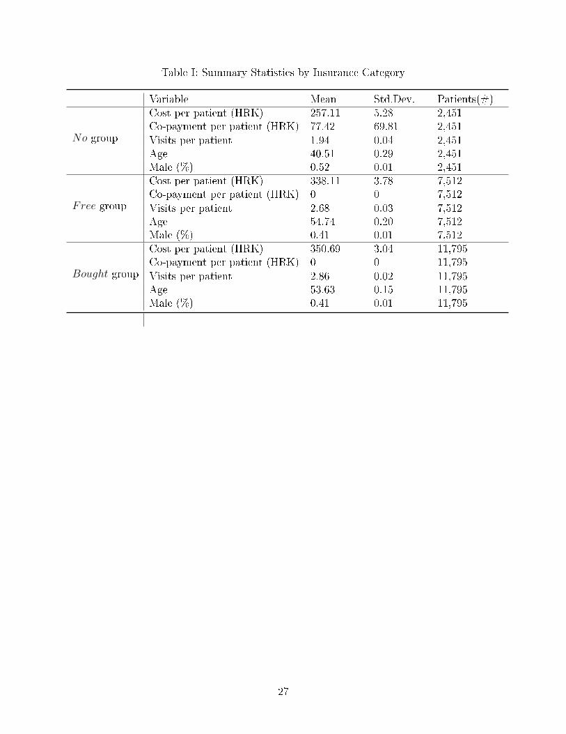
Table I: Summary Statistics by Insurance Category

Variable Mean Std.Dev. Patients(#)Cost per patient (HRK) 257.11 5.28 2,451Co-payment per patient (HRK) 77.42 69.81 2,451

No group Visits per patient 1.94 0.04 2,451Age 40.51 0.29 2,451Male (%) 0.52 0.01 2,451Cost per patient (HRK) 338.11 3.78 7,512Co-payment per patient (HRK) 0 0 7,512

Free group Visits per patient 2.68 0.03 7,512Age 54.74 0.20 7,512Male (%) 0.41 0.01 7,512Cost per patient (HRK) 350.69 3.04 11,795Co-payment per patient (HRK) 0 0 11,795

Bought group Visits per patient 2.86 0.02 11,795Age 53.63 0.15 11,795Male (%) 0.41 0.01 11,795

27

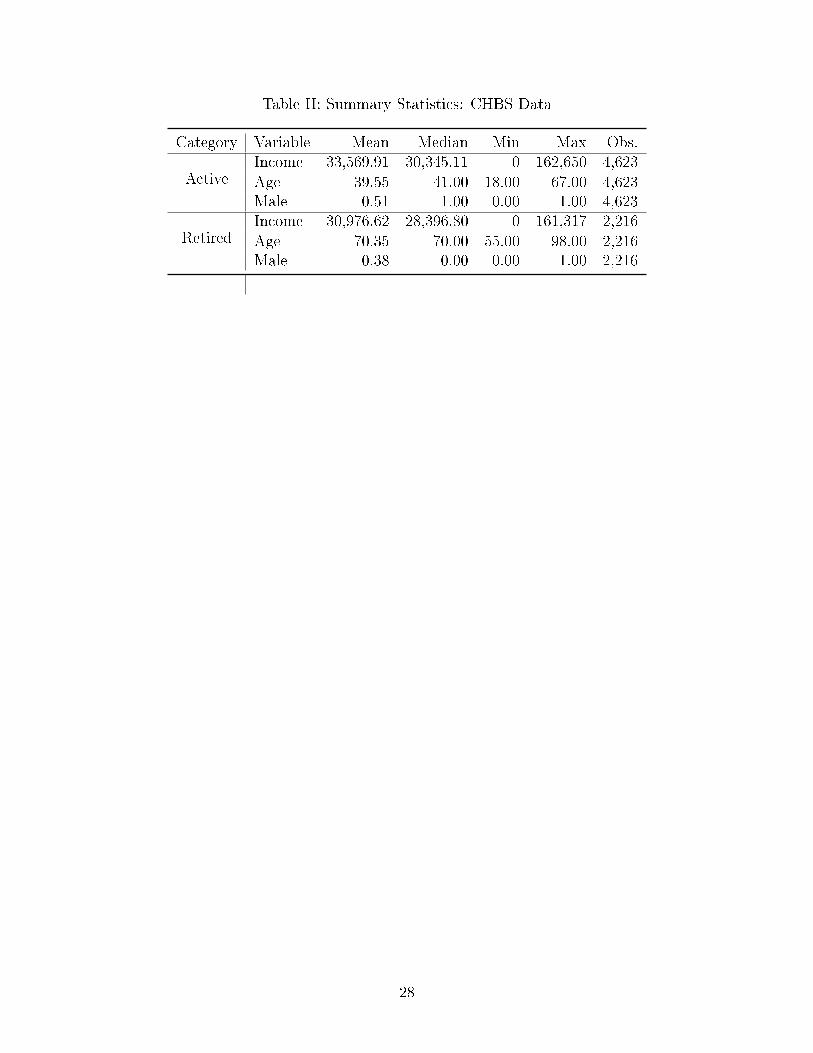
Table II: Summary Statistics: CHBS Data

Category Variable Mean Median Min Max Obs.Income 33,569.91 30,345.11 0 162,650 4,623

Active Age 39.55 41.00 18.00 67.00 4,623Male 0.51 1.00 0.00 1.00 4,623Income 30,976.62 28,396.80 0 161,317 2,216

Retired Age 70.35 70.00 55.00 98.00 2,216Male 0.38 0.00 0.00 1.00 2,216

28

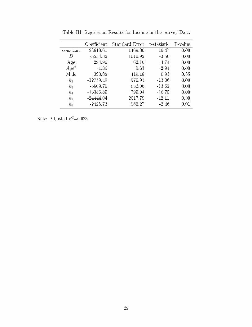
Table III: Regression Results for Income in the Survey Data

Coe�cient Standard Error t-statistic P-valueconstant 28618.61 1469.80 19.47 0.00

D -3534.32 1010.92 -3.50 0.00Age 294.96 62.16 4.74 0.00Age2 -1.86 0.63 -2.94 0.00Male 390.88 419.18 0.93 0.35k2 -12759.49 976.95 -13.06 0.00k3 -8609.76 632.06 -13.62 0.00k4 -13386.89 799.04 -16.75 0.00k5 -24444.04 2017.79 -12.11 0.00k6 -2425.73 986.27 -2.46 0.01

Note: Adjusted R2=0.083.

29

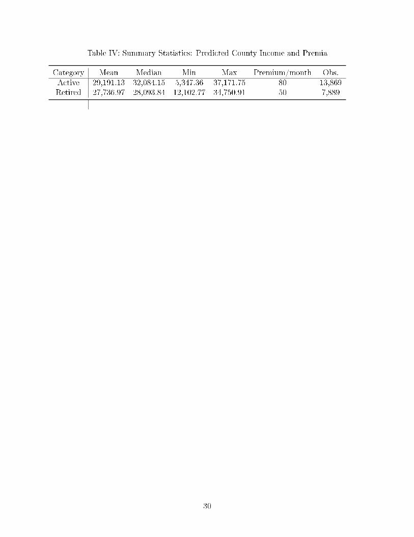
Table IV: Summary Statistics: Predicted County Income and Premia

Category Mean Median Min Max Premium/month Obs.Active 29,191.13 32,084.15 5,347.36 37,171.75 80 13,869Retired 27,736.97 28,093.84 12,102.77 34,750.91 50 7,889

30

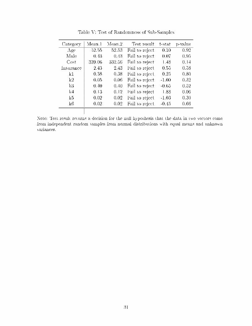
Table V: Test of Randomness of Sub-Samples

Category Mean.1 Mean.2 Test result t-stat p-valueAge 52.55 52.53 Fail to reject 0.10 0.92Male 0.43 0.43 Fail to reject 0.07 0.95Cost 339.06 332.56 Fail to reject 1.48 0.14

Insurance 2.43 2.43 Fail to reject 0.55 0.58k1 0.38 0.38 Fail to reject 0.25 0.80k2 0.05 0.06 Fail to reject -1.00 0.32k3 0.40 0.40 Fail to reject -0.65 0.52k4 0.13 0.12 Fail to reject 1.88 0.06k5 0.02 0.02 Fail to reject -1.03 0.30k6 0.02 0.02 Fail to reject -0.45 0.66

Note: Test result returns a decision for the null hypothesis that the data in two vectors come

from independent random samples from normal distributions with equal means and unknown

variances.

31

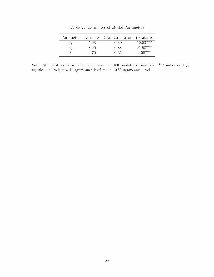
Table VI: Estimates of Model Parameters

Parameter Estimate Standard Error t-statisticγ1 5.98 0.30 19.93***γ2 8.20 0.38 21.58***t 2.70 0.66 4.09***

Note: Standard errors are calculated based on 100 bootstrap iterations. *** indicates 1 %

signi�cance level; ** 5 % signi�cance level and * 10 % signi�cance level.

32

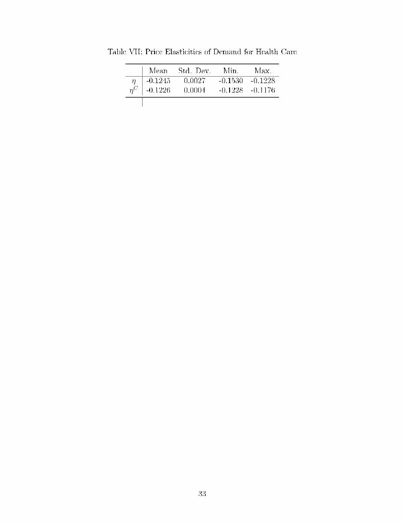
Table VII: Price Elasticities of Demand for Health Care

Mean Std. Dev. Min. Max.η -0.1245 0.0027 -0.1530 -0.1228ηC -0.1226 0.0004 -0.1228 -0.1176

33

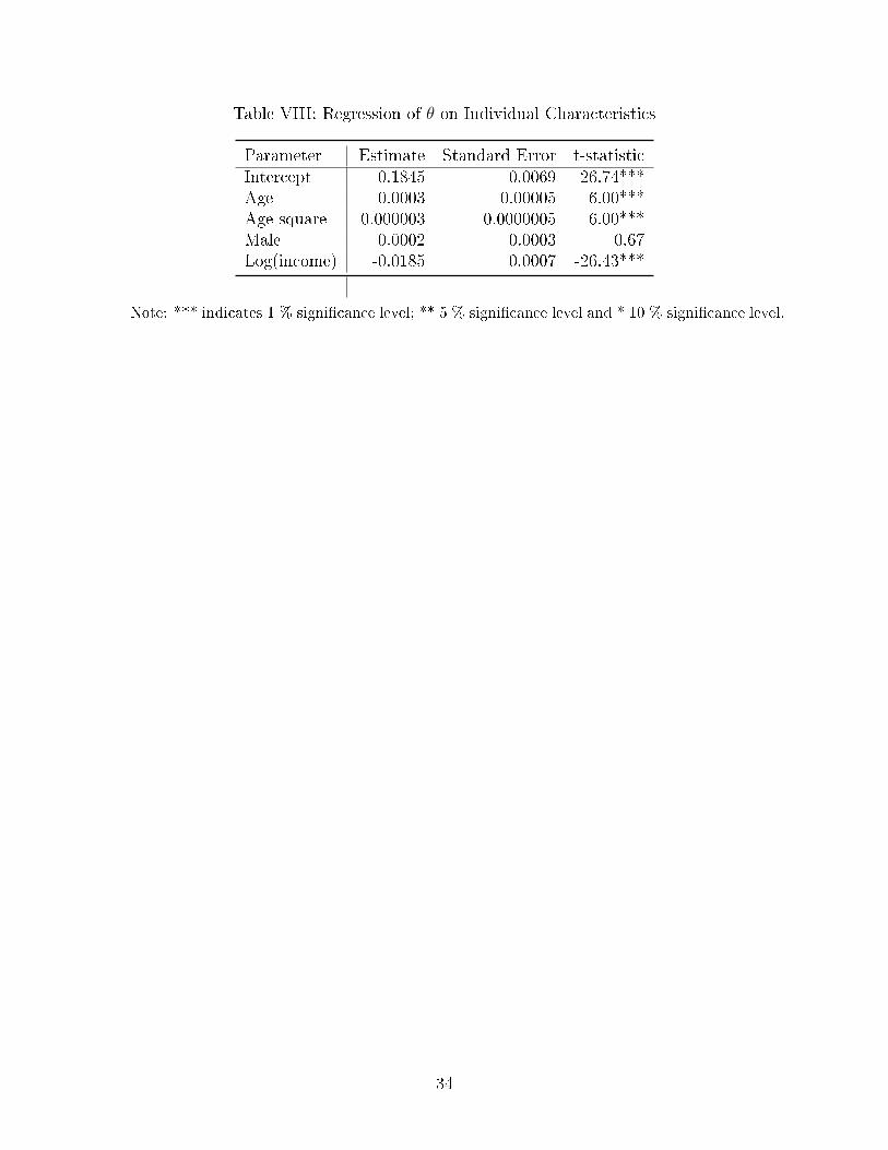
Table VIII: Regression of θ on Individual Characteristics

Parameter Estimate Standard Error t-statisticIntercept 0.1845 0.0069 26.74***Age 0.0003 0.00005 6.00***Age-square -0.000003 0.0000005 -6.00***Male 0.0002 0.0003 0.67Log(income) -0.0185 0.0007 -26.43***

Note: *** indicates 1 % signi�cance level; ** 5 % signi�cance level and * 10 % signi�cance level.

34

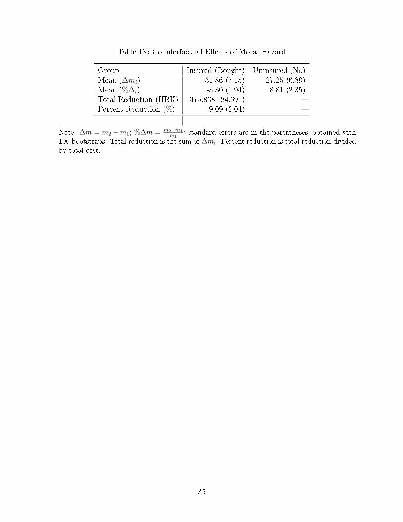
Table IX: Counterfactual E�ects of Moral Hazard

Group Insured (Bought) Uninsured (No)Mean (∆mi) -31.86 (7.15) 27.25 (6.89)Mean (%∆i) -8.30 (1.94) 8.81 (2.35)Total Reduction (HRK) -375,838 (84,691) �Percent Reduction (%) 9.09 (2.04) �

Note: ∆m = m2 −m1; %∆m = m2−m1m1

; standard errors are in the parentheses, obtained with

100 bootstraps. Total reduction is the sum of ∆mi. Percent reduction is total reduction divided

by total cost.

35

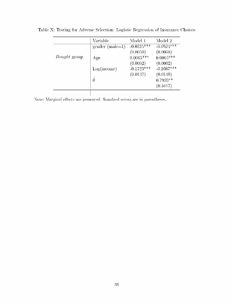
Table X: Testing for Adverse Selection: Logistic Regression of Insurance Choices

Variable Model 1 Model 2gender (male=1) -0.0525***

(0.0059)-0.0524***(0.0059)

Bought group Age 0.0065***(0.0002)

0.0065***(0.0002)

Log(income) -0.1723***(0.0147)

-0.1667***(0.0148)

θ̂ 0.7970**(0.3417)

Note: Marginal e�ects are presented. Standard errors are in parentheses.

36

Table XI: Tests of Adverse Selection: K-S Statistics for equality of θ distribution for No andBought

Group (No and Bought) Statistics P-value ResultsTwo-sided 0.159 0.000 RejectOne-sided 0.159 0.000 Reject

37

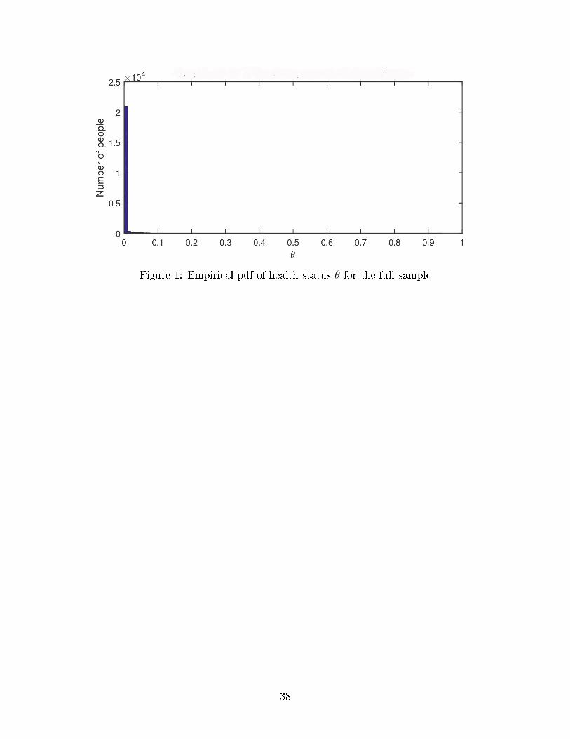
Figure 1: Empirical pdf of health status θ for the full sample

38

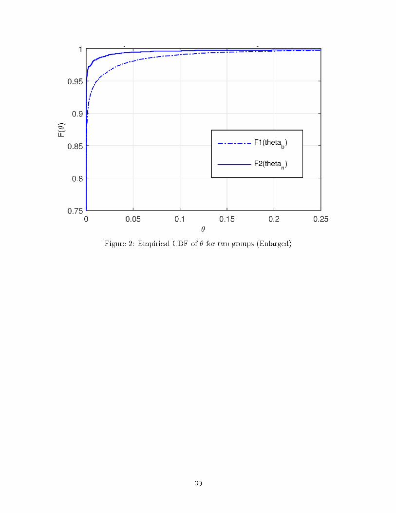
Figure 2: Empirical CDF of θ for two groups (Enlarged)

39

References

Bajari, Patrick, Han Hong, Ahmed Khwaja, and Christina Marsh (2014), �Moral Hazard,

Adverse Selection and Health Expenditures: A Semiparametric Analysis." The Rand Journal

of Economics, 45(4): 747-763.

Cameron, A. C., P. K. Trivedi, Frank Milne and J. Piggott (1988), �A Microeconometric

Model of the Demand for Health Care and Health Insurance in Australia." The Review of

Economic Studies 55(1): 85-106.

Cardon, James H., and Igal Hendel (2001), �Asymmetric Information in Health Insurance:

Evidence from the National Medical Expenditure Survey." The RAND Journal of Economics

32(3): 408-427.

Cutler, D. and R. Zeckhauser (2000), �The Anatomy of Health Insurance." In Handbook of

Health Economics Vol. 1A edited by A.J. Culyer and J.P. Newhouse, 563-644. Amsterdam:

North Holland.

Einav, L., A. Finkelstain, S.P. Ryan, P. Schrimpf and M.R. Cullen (2013), �Selection on

Moral Hazard in Health Insurance." The American Economic Review 103(1): 178-219.

Fang, Hanming, Michael P. Keane, and Dan Silverman (2008), �Sources of Advantageous

Selection: Evidence from the Medigap Insurance Market." Journal of Political Economy

116(2): 303-350.

Gardiol, Lucien, Pierre-Yves Geo�ard, and Chantal Grandchamp (2005), �Separating Selec-

tion and Incentive E�ects in Health Insurance." CEPR Discussion Papers No. 5380.

Greene, W.H. (2002), Econometric Analysis, 5th edition, Prentice Hall.

Liu, X., D. Nestic, and T. Vukina (2012), �Estimating Adverse Selection and Moral Hazard

E�ects with Hospital Invoices Data in a Government-Controlled Healthcare System." Health

Economics 21(8): 883-901.

40

Manning, Willard G., Joseph P. Newhouse, Naihua Duan, Emmett B. Keeler and Arleen

Leibowitz (1987), �AssociationHealth Insurance and the Demand for Medical Care: Evidence

from a Randomized Experiment." The American Economic Review 77(3): 251-277.

Olivella, Pau and Marcos Vera-Hernandez (2013), �Testing for Asymmetric Information in

Private Health Insurance." The Economic Journal 123(567): 96-130.

Paully, M. (1968) �The Economics of Moral Hazard: Comment." The American Economic

Review 58(3): 531-537.

Vera-Hernandez, Marcos (2003), �Structural Estimation of a Principal-Agent Model: Moral

Hazard in Medical Insurance." The RAND Journal of Economics 34(4): 670-693.

Wolfe, John R., and John H. Goddeeris (1991), �Adverse Selection, Moral Hazard, and

Wealth E�ects in the Medigap Insurance Market." Journal of Health Economics 10(4): 433-

459.

41