ERROR ESTIMATION PROCEDURES FOR MONTE CARLO COMPUTATIONS © M. Ragheb 3/16/2013 INTRODUCTION

All measured data, whether in actual experiments, sampling and inspection, or numerical computations are subject to error. The error could be random from unknown or uncontrollable causes. It could be systematic from consistent and more controllable origins. An objective of any error estimation method is to provide consistency or uniformity from one test to the next on the same object that is being sampled. To achieve this objective it is necessary to understand what causes variability in measurements, and what the limits of control are. The goal is to understand how to make a given measurement as accurate and precise as possible, and to understand the occurrence of the unavoidable random error.

We present a recursive procedure to estimate the error as a Monte Carlo simulation is underway which allows the stopping of the computation once a desired pre-assigned level of computational error is attained. The error estimate is obtained on a recursive basis involving the addition of two quantities at each step, thus reducing the error buildup. TYPES OF ERROR

In this context some important concepts must be understood: Accuracy: is the degree of agreement between the measured result and the true answer. Precision: is the ability of a measuring system to repeat the same result. Bias: is a consistent error in one direction between two measures. The general concept of experimental error can be subdivided into three broad types: 1. Random, or accidental error, having four meanings in use:

i) Deviations or statistical fluctuations around the mean. ii) Random error, which refers to the arithmetic mean’s, that is obtained

through averaging over a number of random trials, deviation from the mean determined from a larger number of trials, or sometimes the true or parent mean.

iii) Statistical error, which is a measure of the reliability of a measurement such as the standard deviation.

iv) Elementary error like the de effect of Brownian motion on a torsion balance.

2. Systematic error, which is an error which tends to have the same algebraic sign. This can be a bias or a truncation. 3. Blunders, which are outright mistakes. A measurement known to contain blunders should be either corrected or discarded.

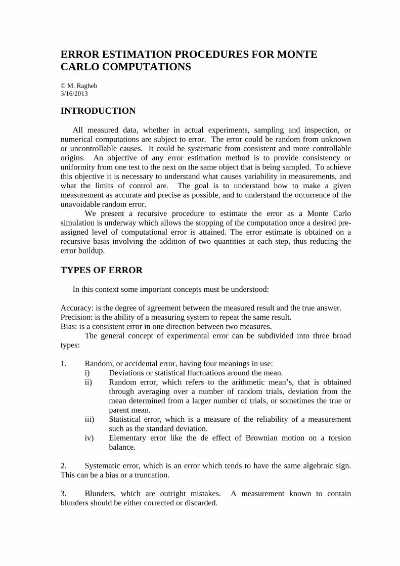
A Monte Carlo calculation being a numerical experiment, one must maximize the precision which proportional to the reciprocal of the statistical error, and the accuracy by making the net systematic error as small as achievable. Statistical theory deals extensively with these subjects, but Monte Carlo users did not take full advantage of it. We outline the methods used in practical Monte Carlo applications for the estimation of the confidence intervals and statistical error. CONFIDENCE INTERVALS Many random events are distributed according to the Normal or Gaussian distribution. Which produces a bell shaped curve as shown in Fig. 1. The highest probability of occurrence is at the mean or average value, with a declining probability of occurrence away from the average.

Figure 1. Normal or Gaussian distribution. In statistical terminology, errors as differences from the average or true mean are quantified as variances, which are the square of the difference between the obtained result and the calculated average value. The average squared deviation is the variance for a system. Its square root is the commonly used parameter designated as standard deviation. The interpretation of the meaning of the standard deviation can be grasped from Fig. 1. About two thirds or 68.3 percent of the values of tests would lie within the range of plus and minus one single standard deviation. About 95 percent of the observations lie within two standard deviations, and 99.7 percent of the observation would lie within 3 standard deviations. A design definition for evaluating tolerances can be set for comparing the bias against the random error. One can require that the measured values must compare within a given number of standard deviations, or they are not equivalent. The number of standard deviations is determined by the willingness to accept the risk of either passing a poor test or of failing a good one. This leads to the concept of confidence levels. The range from minus 2 standard deviations to plus 2 standard deviations, leads to a 95 percent confidence that the true mean lies anywhere between these two limits. Because the variance is an average squared deviation, the more measurements are included, the greater the precision and the smaller the tolerance. This is shown in Fig. 1 where the results from the average of multiple tests lead to a narrowing of the Normal distribution with smaller variance. While more measurements reduce the random error, there may be a diminishing return as more data at an extra cost is generated.

In system design, the goal is to minimize the total variance. This means that we get estimates from each measurement and then add them. Notice that the variances from individual sources add up. However, the standard deviations do not. In Monte Carlo simulations the goal is to also minimize the total variance in the estimate, hence the importance of the techniques of variance reduction. THE CENTRAL LIMIT THEOREM This theorem has first been given by Laplace and then generalized by Chebyshev, Markov and Lyapunov. The theorem states that: “Let x1, x2, x3,…,xn denote the items of a random sample from a distribution, which has a mean m and positive variance σ2. Then, the random variable:

( )

1

1

1

n

ii

n

n

ii

n

x nmY

n b

xm

nb

nn x m

b

=

=

−=

⋅

−=

⋅

−=

∑

∑ (1)

where:

n

xx

n

ii

n

∑== 1

has a limiting distribution, which is normal with mean m and variance b2.” In other words, the sum of the random variables xi is normally distributed. The validity of the theorem extends to the general condition in which the xi's are not required to be identical and independent. It is only needed that none of them adds too great a contribution to the sum nx . This theorem explains the common occurrence of the normal random variables in nature: aggregate effects of a large number of negligible random factors lead to resulting normal random variables, e.g. the deviation of a cannon shell away from its target. A Normal or Gaussian random variable ξ is defined over the interval: [ ]+∞∞−∈ ,x , and is given by:

( )( )2

2212

x u

p x e σ

π σ

−−

=⋅

(2)

It can be proved that:

( )( ) 2σξ

µξ

=

=

VM

and the proability:

( )∫+

−

=

σµ

σµ

3

3

997.0dxxp (3)

or: 3 3 0.997P µ σ ξ µ σ− < ≤ + = (4) Let us consider identical independent random variables xi, i=1, 2, 3, … , n, whose probability distributions coincide, thus their means and variances also coincide: ( ) ( ) ( ) mxMxMxM n ==== ...21 (5) ( ) ( ) ( ) 2

1 2 ... nV x V x V x b= = = = (6) Consider the sum of the random variables:

∑=

=++++=n

iin xxxxxn

1321 ...

we can write: ( ) ( ) ( ) ( ) ( ) nmxMxMxMxMnM n =++++= ...321 ( ) ( ) ( ) ( ) ( ) 2

1 2 3 ... nV n V x V x V x V x nb= + + + + = If we consider a normal random variable with the same parameters: nm=µ (7) 22 nb=σ (8) According to the Central Limit Theorem and Eq. 4: 3 3 0.997P nm n b nm n bη− ⋅ < ≤ + ⋅ =

Dividing by n, we get the inequality:

! over the unit interval is used, and ensuing distribution ! is constructed. ! M. Ragheb program Central_Limit_Theorem dimension x(100), freq(100) integer :: trials = 100000 integer :: subdivisions = 20 integer :: nvar=4 real x,freq,sum,width width=1.0/subdivisions ! Initialize frequency distribution do i=1,subdivisions freq(i)=0.0 end do ! Initialize scoring bins boundaries do i=1,subdivisions xi=i x(i)=xi/subdivisions end do ! open output file open(44, file = 'random_out') ! Generate sum of uniformly distributed random variables do i= 1, trials sum=0.0 do k=1,nvar call random(rr) sum=sum+rr end do sum=sum/nvar if(sum.LE.x(1))then freq(1)=freq(1)+1.0 end if do j=1,subdivisions if((sum.GT.x(j)).AND.(sum.LE.x(j+1)))then freq(j+1)=freq(j+1)+1.0 end if end do end do ! Normalize frequency distribution do i=1,subdivisions freq(i)=freq(i)/trials end do ! Write results to output file do i=1,subdivisions write (44,100) x(i), freq(i) write(*,*) x(i),freq(i) end do 100 format (2e14.8) end

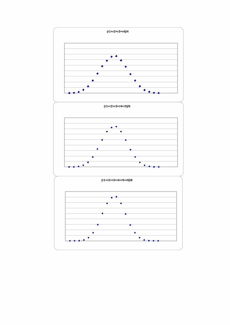
Figure 2. Procedure for the generation of average sums of random variables as a demonstration of the Central Limit Theorem.

r1

(r1+r2)/2

(r1+r2+r3)/3

(r1+r2+r3+r4)/4

(r1+r2+r3+r4+r5)/5

(r1+r2+r3+r4+r5+r6)/6

Figure 3. Plots of the average sums of random variables from n=1 to n=7, for a random variable uniformly distributed over the unit interval. The sum converges into a Gaussian

distribution according to the Central Limit Theorem. Number of trials per experiment=100,000.

SINGLE-BATCH ESTIMATION OF THE SAMPLE VARIANCE Following the analysis in Spanier and Gelbard, let Ω be the space of points for some statistical experiment, and ξ a random variable overΩ . If n independent trials are made, we can define n independent variables nξξξξ ,...,,, 321 on nΩ by: ( ) ( )1 3, , ,...,i w n iw w w w wξ ξ= , ni ≤≤1 . (11) If the random variable ξ has a distribution F, then so does each variable iξ . For a sequence of points w1, w2, w3, … of Ω , the numbers ( ),11 wx ξ= ( ),22 wx ξ=

( ),33 wx ξ= … are a sequence of sample values drawn from the distribution F. For fixed n and each non negative integer ℓ, the random variable:

∑=

=n

iin 1

1

ξα ℓ=0, 1, 2, … (12)

is defined on the space nΩ . For each sequence w1, w2, w3, ... , wn of n points of Ω (corresponding to n trials of the experiment), the value of

α at (w1, w2, w3,...,wn):

( )11

1,...,n

n ii

w w xn

α=

= ∑

(13)

where ( )i ix wξ= is called the -th sample moment of the sample values x1, x2, x3,...,xn. For every , this number can be regarded as the -th moment of a discrete

distribution F*(x) defined by placing a weight of a 1n

at each of the points xi, 1 i n≤ ≤ .

(r1+r2+r3+r4+r5+r6+r7)/7

as an estimate of τ1. In practice, especially in Monte Carlo applications, σ is also unknown. So we are led to use sample estimators to give an approximation to the expected errors. The random variable 2

2 1α α− , whose value is a sequence ( )1 2, ,..., nw w w of trials, is the sample variance:

( )( )2 2

2 1 1 2

22

1 1

, ,...,

1 1

n

n n

i ii i

s w w w

x xn n

α α

= =

= −

= −

∑ ∑ (19)

might be used to estimate the population variance σ2 since it converges in measure to σ2, thus we say that 2

2 1α α− is a consistent estimator of σ2. For small size samples, however, the expected value of 2

2 1α α− is not the population variance σ2 but the smaller biased value:

21nn

σ−

,

instead. This fact can be proven as follows. Let:

( )2 22 21 1i i

i is x x x x

n n= − = −∑ ∑

Placing the origin at the mean of the population, since any central sample moment is independent of the origin on the scale of variable, then:

2 2 2

2 2 21( ) n nE sn n n nσ σ σσ σ−

= − = − =

This may be corrected by replacing the estimate 22 1α α− by ( )2

2 11n

nα α ⋅ − −

to

correct the bias, thus:

( )2 22 11

nEn

α α σ ⋅ − = − (20)

Applying the correction to eliminate the bias, the unbiased estimate of the popupulation variance becomes a correction of Eqn. 19:

( )

( )

22

2 1 1

2

2 1

1

1

11

n n

i ii i

n

ini

ii

x xnS

n n n

xx

n n

= =

=

=

= − −

= − −

∑ ∑

∑∑

(21)

which is an unbiased and consistent estimator of the population variance. Another form of Eq. 19 for the sample variance can be written as:

2

2 1

1

1

n

ini

ii

xs x

n n=

=

= −

∑∑ (19)’

which is a consistent (but biased) estimator of σ2. To get a consistent and unbiased estimate of σ2 we write the equivalent to Eq. (21) by multiplying by n / (n-1):

( )

2

2 1

1

11

n

ini

ii

xS x

n n=

=

= −

−

∑∑ (21)’

giving an estimate S for σ, from which we can calculate the standard error of the average

value as nσ as shown in the next section.

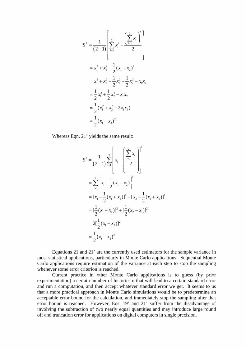
EXAMPLE For n = 2, Eqn. 21 yields:

( )

22

22 2 1

1

2 2 21 2 1 2

2 2 2 21 2 1 2 1 2

2 21 2 1 2

2 21 2 1 2

21 2

12 1 2

1 ( )21 12 2

1 12 21 ( 2 )21 ( )2

ii

ii

xS x

x x x x

x x x x x x

x x x x

x x x x

x x

=

=

= − −

= + − +

= + − − −

= + −

= + −

= −

∑∑

Whereas Eqn. 21’ yields the same result:

( )

22

22 1

1

22

1 21

2 21 1 2 2 1 2

2 21 2 2 1

21 2

21 2

12 1 2

1 ( )2

1 1[ ( )] [ ( )]2 2

1 1[ ( )] [ ( )]2 2

12[ ( )]2

1 ( )2

ii

ii

ii

xS x

x x x

x x x x x x

x x x x

x x

x x

=

=

=

= −

−

= − +

= − + + − +

= − + −

= −

= −

∑∑

∑

Equations 21 and 21’ are the currently used estimators for the sample variance in most statistical applications, particularly in Monte Carlo applications. Sequential Monte Carlo applications require estimation of the variance at each step to stop the sampling whenever some error criterion is reached. Current practice in other Monte Carlo applications is to guess (by prior experimentation) a certain number of histories n that will lead to a certain standard error and run a computation, and then accept whatever standard error we get. It seems to us that a more practical approach in Monte Carlo simulations would be to predetermine an acceptable error bound for the calculation, and immediately stop the sampling after that error bound is reached. However, Eqs. 19’ and 21’ suffer from the disadvantage of involving the subtraction of two nearly equal quantities and may introduce large round off and truncation error for applications on digital computers in single precision.

DERIVATION OF A PROPOSED RECURSIVE FORMULA FOR THE ESTIMATION OF THE VARIANCE We deduce here a third formula for the estimation of the variance where we get our result on a recursive basis, involving the addition of two quantities at each step, thus reducing the error buildup problem. The formula is exposed here for the benefit of the interested reader and user. It bears semblance to Sequential Monte Carlo calculations. For the k-th history, trial, or experiment, the unbiased and consistent estimator of σ2 is from Eq. 21’:

( )

2

2

1 1

1 11

k k

k i ji j

S x xk k= =

= − −

∑ ∑ , (22)

whilst for the (k-1)-st step it is:

( ) ( )

21 1

21

1 1

1 12 1

k k

k i ji j

S x xk k

− −

−= =

= − − −

∑ ∑ (22)’

Equation 22 can be rewritten as:

( )

2 21 1

2

1 1 1

1 1 11

k k k

k i j k ji j j

S x x x xk k k

− −

= = =

= − + − − ∑ ∑ ∑ (22)”

Subtracting Eqn. 22’ from Eqn. 22” we get:

( ) ( ) ( )

2 2 21 1 1

2 21

1 1 1 1 1

1 1 11 21

k k k k k

k k i j i j k ji j i j j

k S k S x x x x x xk k k

− − −

−= = = = =

− = − − − + − + − −

∑ ∑ ∑ ∑ ∑

Combining the second and third terms on the Right Hand Side (RHS):

( ) ( ) ( )

22 21 1

2 21

1 1 1 1

1 1 11 21

k k k k

k k i j i j k ji j j j

k S k S x x x x x xk k k

− −

−= = = =

− = − + − − − + − −

∑ ∑ ∑ ∑

Using the identity: ( ) ( )2 2a b a b a b− = + ⋅ − , we get:

( ) ( ) ( ) ( )1 1 1

2 21

1 1 1 1 1

2

1

1 1 1 11 2 21 1

1

k k k k k

k k i j j j ji j j j j

k

k jj

k S k S x x x x xk k k k

x xk

− − −

−= = = = =

=

− = − + − − ⋅ − + − −

+ −

∑ ∑ ∑ ∑ ∑

∑

Using the relation:

1

1 1

k k

j j kj j

x x x−

= =

= +∑ ∑

thus:

( ) ( ) ( )1 1 1 1 1

2 21

1 1 1 1 1

21

1

1 1 1 11 2 21 ( 1)

1

k k k k kk k

k k i j j j ji j j j j

kk

k jj

x xk S k S x x x x xk k k k k k

xx xk k

− − − − −

−= = = = =

−

=

− = − + − − − ⋅ − + − − −

+ − −

∑ ∑ ∑ ∑ ∑

∑

Denoting:

( ) ( )

1

11

1 11

1 ,1

k

j kj

k i ki

xt x k t

k

−

−=

− −=

= → = −−

∑∑ 1k ≠ (23)

we get:

( ) ( )1

2 21 1 1 1 1

1

2

1

1 11 2 2

1 1 , 1

kk k

k k i k k k ki

k k

x xk kk S k S x t t t tk k k k

k kx t kk k

−

− − − − −=

−

− − − = − + − − − ⋅ − −

− − + − ≠

∑

Since:

( ) ( )1 1 1

,n n n

i i ii i i

ax b c c ax b c a x nb= = =

+ = + = + ∑ ∑ ∑

we have:

( ) ( ) ( ) ( ) ( )

( ) ( ) ( ) ( )

( ) ( ) ( ) ( )

2122 2

1 1 1 121

2122

1 1 1 11

21 1 1

1 2 111 2 2

1 (1 2 ) 12 2 1

112 2 1

kk k

k k i k k k ki

kk

k k k i k k ki

k k k k

k kx xk S k S x t t x tk k k k k

xk kk S t x x k t x tk k k k

kk S t x k t

k k

−

− − − −=

−

− − − −=

− − −

− − − = − + − − ⋅ − + −

− − = − + − + − ⋅ − + ⋅ −

−= − + − − +

∑

∑

( ) ( ) ( )

( ) ( ) ( ) ( ) ( )

( ) ( ) [ ]

2

1 1

222

1 1 1 1

221 1

1 11 2

11 12

12

k k k k

k k k k k k k

k k k

k kk t x x tk k

k kk S t x t x x tk k kk

k S t xk

− −

− − − −

− −

− − − − + −

− − = − + − ⋅ − + −

−= − + −

Leading to the simple recursive formula:

( )( ) ( )22 2

1 1

2 1 , 11k k k k

kS S t x k

k k− −

−= + − ∀ ≠

− (24)

where: ( )

1

11 ,

1

k

ii

k

xt

k

−

=− =

−

∑ and with: 2

1 0.0.S =

Equation 24 can be written in the form:

( )( ) ( )2 2 2 2

1 1 1

2 1 21k k k k k k

kS S t x x t

k k− − −

−= + + −

− (24)’

Equations 24, 19’ and 21’ for S2 are equivalent, with the estimation carried out on a recursive basis. For the special case of k=2 (noting that 2

1 0.0S = ) from Eq. 24:

( )221 1 2 1 2

10.02

t x S x x= → = + −

while from Eq. 21’:

( ) ( )2 2 22

21 22 1 2 2 12 1 2

1

12 2 2 2i

i

x x x x x xS x x x=

+ − − = − = + = −

∑ ,

which proves their equivalence for k = 2. ESTIMATION OF THE STANDARD DEVIATION OF THE SAMPLE MEAN The sample mean is defined as:

Clark has analyzed the use of this method for Monte Carlo, and his analysis is implied in many Monte Carlo codes, where a batch is referred to as a statistical aggregation. It is often referred to as an experiment, and confidence limits are deduced from batch values. Suppose the sample of size n is cut into k equal samples, each of size : n = k . To each of the k batches one can compute a mean value:

1

1 ,lm jmj

x x=

= ∑

m = 1, 2, 3, ... , k (27)

where xjm are the item samples in the m-th batch. The mean of the entire sample is:

1

1 k

n mm

x xk =

= ∑

(28)

The means of samples of size have a distribution whose standard distribution can be computed as:

[ ]2

2

1

1 k

n mm

s x xk =

= −∑

(29)

The expectation value of the square of the corresponding population standard deviation is:

2 2

1k s

kσ =

−

(30)

The squared standard deviation of the mean computed from k independently determined values of mx

(i.e. of a sample of size k of the objects mx

) is:

2 21n k

σ σ=

(31)

and:

( )( )

22

1 1

kn m

nm

x xk k

σ=

−=

−∑ (32)

The use of the batch method is recommended where splitting of particles in a calculation is significant. The working formula for batch statistics used in this case is:

2

2 22

1 1

1 1 11

N N

x i i i ij j

n x n xN n n

σ= =

= − − ∑ ∑ (33)

where: N = number of batches

n = total number of independent histories ni = number of independent histories in the i-th batch xi = accumulated estimate in i-th batch, with:

1

N

ii

n n=

=∑ , 1

1 in

i ijjj

x xn =

= ∑ (34)

where xij is the estimate from the i-th history in the i-th batch:

1

1 N

i ii

x n xn =

= ∑ (35)

where x is the mean, averaged over n histories. The fractional standard deviation of Eqn. 26 is used as:

2x xfsd

x xσ σ

= = (26)’

DISCUSSION The Monte Carlo method, being a stochastic process, offers an advantage compared with other numerical methods, in that an estimate of the calculation error is generated as the calculation proceeds. It also offers the ability to test the attained error at different steps, and stopping the calculation whence the accepted error level is reached. Several methods exist for error estimation in Monte Carlo simulations, and the choice of one method or the other depends on the context in which it is being used and the preference of the user. As the error is inversely proportional to the square root of the number of trials or experiments, decreasing the error by one half requires the quadrupling of the number of trials. This should not be solely depended upon as away of decreasing the error in Monte Carlo simulations. The most efficient way of decreasing the error in Monte Carlo simulations is to take notice of the fact that the error is proportional to the variance of the sampling scheme. One can thus efficiently minimize the variance by altering the sampling scheme while keeping the same means of the sampled process. This is the realm of Monte Carlo Variance reduction methods. We present a recursive procedure to estimate the error as a Monte Carlo simulation is underway which offers the advantage of the capability of stopping of the computation once a desired pre-assigned level of computational error is attained. In addition, the error estimate is obtained on a recursive basis involving the addition of two quantities at each step, thus reducing the error buildup in the final estimate. APPENDIX: ACCURACY AND PRECISION Monte Carlo simulations aim at both accuracy and precision. The terms “accuracy” and “precision” are used interchangeably. However, for the technical and scientific fields, these words have different meanings. “Accuracy” refers to how closely a measurement or observation comes to measuring a "true value," since measurements

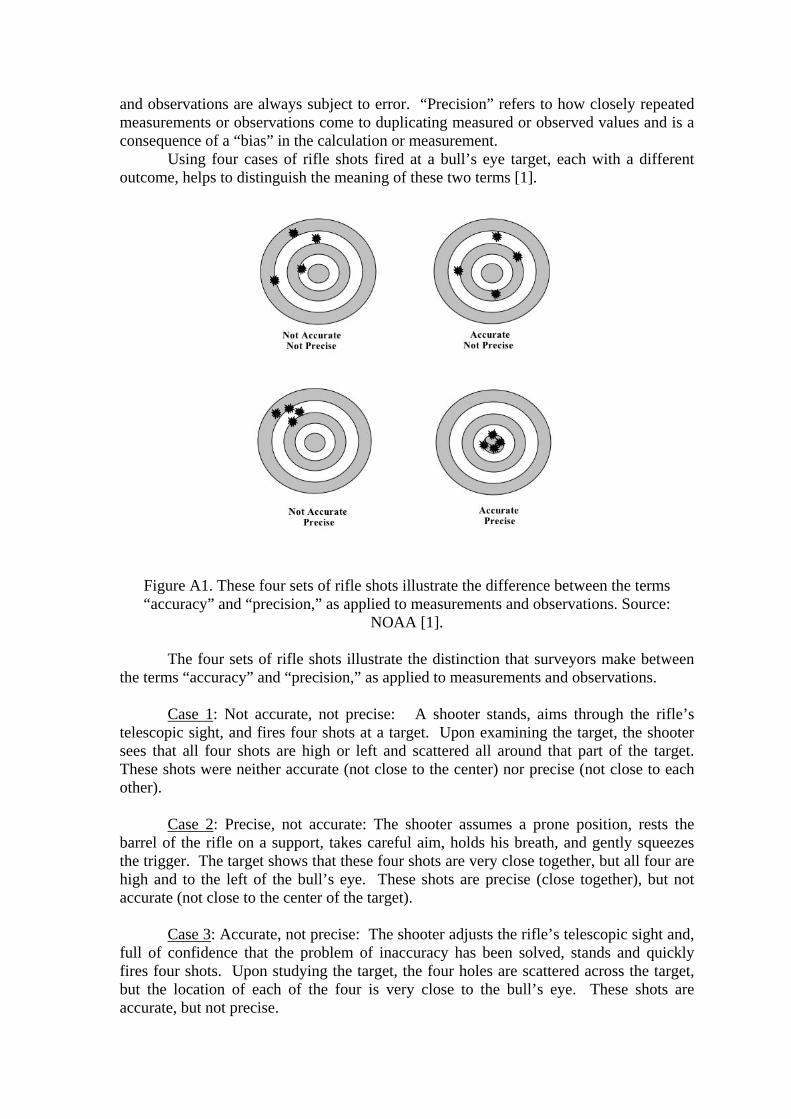
and observations are always subject to error. “Precision” refers to how closely repeated measurements or observations come to duplicating measured or observed values and is a consequence of a “bias” in the calculation or measurement. Using four cases of rifle shots fired at a bull’s eye target, each with a different outcome, helps to distinguish the meaning of these two terms [1].

Figure A1. These four sets of rifle shots illustrate the difference between the terms “accuracy” and “precision,” as applied to measurements and observations. Source:

NOAA [1]. The four sets of rifle shots illustrate the distinction that surveyors make between the terms “accuracy” and “precision,” as applied to measurements and observations. Case 1: Not accurate, not precise: A shooter stands, aims through the rifle’s telescopic sight, and fires four shots at a target. Upon examining the target, the shooter sees that all four shots are high or left and scattered all around that part of the target. These shots were neither accurate (not close to the center) nor precise (not close to each other). Case 2: Precise, not accurate: The shooter assumes a prone position, rests the barrel of the rifle on a support, takes careful aim, holds his breath, and gently squeezes the trigger. The target shows that these four shots are very close together, but all four are high and to the left of the bull’s eye. These shots are precise (close together), but not accurate (not close to the center of the target). Case 3: Accurate, not precise: The shooter adjusts the rifle’s telescopic sight and, full of confidence that the problem of inaccuracy has been solved, stands and quickly fires four shots. Upon studying the target, the four holes are scattered across the target, but the location of each of the four is very close to the bull’s eye. These shots are accurate, but not precise.

Case 4: Accurate, precise: The shooter again assumes a prone position, rests the barrel of the rifle on a support, takes careful aim, holds his breath, and gently squeezes the trigger four times. This time, the four holes are very close to the center of the target (accurate) and very close together (precise). To illustrate the distinction between terms using a surveying context, imagine surveyors very carefully measuring the distance between two survey points about 30 meters (approximately 100 feet) apart 10 times with a measuring tape. All 10 of the results agree with each other to within two millimeters (less than one-tenth of an inch). These would be very precise measurements. However, suppose the tape they used was too long by 10 millimeters. Then the measurements, even though very precise, would not be accurate. Other factors that could affect the accuracy or precision of tape measurements include: incorrect spacing of the marks on the tape, use of the tape at a temperature different from the temperature at which it was calibrated, and use of the tape without the correct tension to control the amount of sag in the tape [1]. REFERENCE 1. ____, “Accuracy Versus Precision,” NOAA Magazine, “NOAA Celebrates 200 Years of Science, Service and Stewardship,” July 19, 2012. PROBLEMS 1. Instead of summing up a uniformly distributed random variable over the unit interval in the numerical test of the central limit theorem, choose any other random variable such as the exponential distribution to test the Normal distribution prediction of the Central Limit Theorem. 2. A method of sampling a normal distribution is to sum a number of uniformly distributed random variables. Vary the number of summed random variables from 1 to 20 to come up with a recommendation about a sufficient number of sums of random variables to generate a stable Normal distribution with unit mean 1 and variance. 3. Use mathematical induction to prove the equivalence of the different formulae used for the estimation of the variance for n = 2 and n = 3.