LUND UNIVERSITY

PO Box 117221 00 Lund+46 46-222 00 00

Error characterization of the Gaia astrometric solution II. Validating the covarianceexpansion model

Holl, Berry; Lindegren, Lennart; Hobbs, David

Published in:Astronomy & Astrophysics

DOI:10.1051/0004-6361/201218808

2012

Link to publication

Citation for published version (APA):Holl, B., Lindegren, L., & Hobbs, D. (2012). Error characterization of the Gaia astrometric solution II. Validatingthe covariance expansion model. Astronomy & Astrophysics, 543, [A15]. https://doi.org/10.1051/0004-6361/201218808

General rightsCopyright and moral rights for the publications made accessible in the public portal are retained by the authorsand/or other copyright owners and it is a condition of accessing publications that users recognise and abide by thelegal requirements associated with these rights.

• Users may download and print one copy of any publication from the public portal for the purpose of private studyor research. • You may not further distribute the material or use it for any profit-making activity or commercial gain • You may freely distribute the URL identifying the publication in the public portalTake down policyIf you believe that this document breaches copyright please contact us providing details, and we will removeaccess to the work immediately and investigate your claim.

A&A 543, A15 (2012)DOI: 10.1051/0004-6361/201218808c© ESO 2012

Astronomy&

Astrophysics

Error characterization of the Gaia astrometric solutionII. Validating the covariance expansion model

B. Holl, L. Lindegren, and D. Hobbs

Lund Observatory, Lund University, Box 43, 22100 Lunde-mail: [Berry.Holl;Lennart.Lindegren;David.Hobbs]@astro.lu.se

Received 11 January 2012 / Accepted 1 May 2012

ABSTRACT

Context. To use the data in the future Gaia catalogue it is important to have accurate estimates of the statistical uncertainties andcorrelations of the errors in the astrometric data given in the catalogue.Aims. In a previous paper we derived a mathematical model for computing the covariances of the astrometric data based on seriesexpansions and a simplified attitude description. The aim of the present paper is to determine to what extent this model provides anaccurate representation of the expected random errors in the astrometric solution for Gaia.Methods. We simulate the astrometric core solution by making least-squares solutions of the astrometric parameters for one mil-lion stars and the attitude parameters for a five-year mission, using nearly one billion simulated elementary observations for a totalof 26 million unknowns. Two cases are considered: one in which all stars have the same magnitude, and another with 30% brighterand 70% fainter stars. The resulting astrometric errors are statistically compared with the model predictions.Results. In all cases considered, and within the statistical uncertainties of the numerical experiments (typically below 0.4%), the theo-retically calculated variances and covariances are consistent with the simulations. To achieve this it is however necessary to expand thecovariances to at least third or fourth order, and to apply a (theoretically motivated and derived) “fudge factor” in the kinematographicmodel.Conclusions. The model provides a feasible method to estimate the covariance of arbitrary astrometric data, accurate enough formost applications, and as such it should be available as part of the user’s interface to the Gaia catalogue. A main assumption in thecurrent model is that the observational errors are uncorrelated (e.g., photon noise), and further studies are needed on how correlatedmodelling errors, in particular in the attitude, can be taken into account.

Key words. astrometry – catalogs – methods: data analysis – methods: statistical – space vehicles: instruments

1. Introduction

Gaia is the European Space Agency astrometric mission sched-uled for launch in 2013. It will observe roughly one billion stars,quasars and other point like objects (hereafter called “sources”),for which the five astrometric parameters (position, parallax andproper motion) will be determined. The Gaia catalogue is ex-pected to become available around 2021. Efficient use of thecatalogue data requires that the astrometric errors are reliablycharacterized, and in particular that the standard uncertainties(or equivalently the variances) are correctly estimated. Whencombining several astrometric parameters their statistical corre-lations (or equivalently the covariances) may also be important.Thus, in general we need to know the full variance-covariancematrix (or covariance matrix for brevity) of all the astrometricparameters. Because of the extremely large number of astromet-ric parameters (∼5×109), the standard method of estimating thecovariance matrix, involving the inversion of an equally largenormal matrix, cannot be applied.

In Holl & Lindegren (2012, Paper I) we derived an approx-imate series expansion model to compute the covariance matrixfor arbitrary subsets of the astrometric parameters (or more gen-erally for arbitrary functions of the astrometric parameters), tak-ing into account the statistical correlations introduced by the at-titude estimation errors. The aim of the present paper is to testthe validity of this model by means of numerical experimentssimulating the astrometric core solution for one million sources.

The model formulated in Paper I uses a “kinematographic”attitude model, where the continuous scanning of Gaia is ap-proximated by a “step and stare” motion. This greatly reducesthe complexity of computing the attitude contribution to thecovariances since each observation is linked to only one atti-tude parameter instead of many, as in the case of a continuous(spline) representation of the attitude. The covariance model al-lows us to approximate the covariance matrix U between allthe source parameters by means of the series expansion U =U(0)+U(1)+U(2)+ · · · (Eq. (19) of Paper I, hereafter I:19), wherethe top “∼” indicates the approximation. In practice we are in-terested in the truncated expansion up to some finite α, denotedby square brackets:

U[α] = U(0) + U(1) + · · · + U(α). (1)

As mentioned in Paper I, we more generally want to characterizethe joint errors of m different scalar quantities y = (y1, . . . , ym)depending on some subset of n astrometric parameters x =(x1, . . . , xn). Introducing the m × n Jacobian matrix J withelements Jμν = ∂yμ/∂xν we have

F ≡ Cov(y) = JUJ ′, (2)

where U = Cov(x) is the covariance matrix of the relevant subsetof astrometric parameters. Using Eq. (1) we can approximateEq. (2) as

F[α] = F(0) + F(1) + · · · + F(α), (3)

Article published by EDP Sciences A15, page 1 of 13

A&A 543, A15 (2012)

where F(α) = JU(α) J ′ for α = 0, 1, . . . The algorithm forthe practical computation of covariances described in Sect. 5 ofPaper I uses this more general formulation. The length of thecomputations increases by a large factor for each higher-orderterm.

The two main issues addressed in this paper concern: (i) thevalidity of the approximations introduced in Paper I, in particu-lar the kinematographic approximation; and (ii) the minimum αneeded for a given relative accuracy of the covariances. They arediscussed in Sect. 4, following a brief description of the numer-ical simulations (Sect. 2) and a discussion of the methodologyfor the numerical validation (Sect. 3).

2. Numerical simulations

2.1. Simulating astrometric solutions using AGISLab

The covariance model developed in Paper I will be validatedthrough a comparison with numerical results simulating the as-trometric solution that is a central part of the Gaia data process-ing. Ideally, the validation should use the models, algorithms andsoftware developed for the analysis of the real Gaia data, knownas AGIS (Astrometric Global Iterative Solution) and comprehen-sively described in Lindegren et al. (2012). For practical rea-sons we use a separate software system called AGISLab, whichhas a subset of the most important functionalities of AGIS,only implemented in a light-weight processing framework moresuitable for small-scale experimental runs on small computers.Importantly, AGISLab adds a number of features specifically de-signed for numerical experiments, in particular on-the-fly gen-eration of simulated input data (“observations”) and the abilityto perform scaled-down experiments (involving much fewer pa-rameters than a minimum AGIS run) in a meaningful way usinga single scaling parameter S (Holl et al. 2010; Bombrun et al.2012). The simulations described in this paper use the observa-tion generator in AGISLab to obtain input data with well-definedstatistical properties, but do not make use of the down-scaling fa-cility in AGISLab; in other words all observations are generatedfor nominal values of the CCD size, focal plane geometry, field-of-view size, satellite spin rate, and scanning law, equivalent toS = 1; see, e.g., Table 1 in Lindegren (2010) for a summary ofthe main mission parameters of Gaia.

Like virtually all Gaia data processing software, AGIS andAGISLab are entirely written in the Java language (O’Mullaneet al. 2011) and make extensive use of the common Java tool-boxes collected and maintained by the Gaia software develop-ment teams. Consistency between AGIS and AGISLab is en-sured by the use of common code for many of the central taskssuch as the calculation of the observation equations and the up-dating of source and attitude parameters. In fact, much of thiscode was first developed and tested in AGISLab before it wasintroduced in AGIS. Thus we are confident that the present simu-lation results, obtained with AGISLab, are in all relevant aspectsequivalent to the corresponding AGIS output.

2.2. Requirements for the simulations

The structure of the normal equations depends strongly on thenumber of source and attitude parameters that are included.Ideally we would like to simulate a realistic AGIS solutionwith the expected 108 primary sources and an attitude modelhaving a spline knot interval in the 5–30 s range as expectedfor the real mission (due to the CCD observations integra-tion time of �4.42 s for the majority of the sources, variationson shorter timescales cannot be distinguished). Given available

computational resources we are able to use a reasonably real-istic attitude knot interval of 30 s but are however restricted toa maximum of 106 sources. Distributing these sources randomlyon the sky results in a mean number density of 24.2 deg−2, whichtranslates into an average of 12 sources simultaneously visible ineach of the two fields of view.

The three-axis attitude of Gaia is reconstructed, as a func-tion of time, by combining across-scan (AC) measurements ofsource positions in the skymappers (SM) of the two fields ofview with along-scan (AL) measurements in the combined as-trometric field (AF). For a 5 yr mission the mean number offield-of-view transits for randomly distributed sources is 88.0(excluding dead-time), corresponding to 16.7 source transitsper 30 s attitude knot interval in the combined fields of view.Because there is typically one AC observation (in the SM) andnine AL observations (in the AF) per transit, this results in16.7 AC observations and 151 AL observations per knot interval,which is sufficient to ensure a proper attitude determination overthe whole mission duration. It is however (almost) necessary thatthe 1 million sources have a uniform random distribution on thesky, rather than following some more realistic (Galactic) den-sity distribution: otherwise there would not be a sufficient num-ber of observations per attitude knot interval when both fieldsof view are looking away from the Galactic plane. We have notconsidered to use a variable knot interval (which to some degreewould circumvent the density problem) because it would lead tounrealistically large intervals part of the time.

Although we are only able to simulate 1% of the expected108 primary sources anticipated for the final astrometric coresolution (Lindegren et al. 2012), the resulting 12 sources perfield of view sample the scanning-law induced structure betweensources on a sufficiently small spatial scale that the resultingconnectivity structure is similar to what we would have for a(much) larger number of sources1. Holl et al. (2010) found thatthe largest correlations between the astrometric parameters ofdifferent sources are obtained for pairs that have an angular sep-aration much less than the field of view, with a maximum corre-lation coefficient inversely proportional to the number of sourcesin the combined fields of view. Since the present experiments usemuch fewer primary sources than the final astrometric solutionfor the Gaia catalogue, the experiments are likely to exaggeratethe correlations by a significant factor.

It is no coincidence that the number of field-of-view tran-sits per attitude interval (∼16) is similar to the mean number ofsources per (combined) field of view (∼24). In simple words onemust determine the next “field pointing” before the current fieldmoves completely out of view. As a field-of-view transit takesabout 43 s, the attitude interval should be of a similar or shorterduration, e.g., the adopted 30 s.

2.3. Simulation experiments

The numerical validation of the covariance model was carriedout for the following two cases:

Case A: 1 million randomly distributed sources of a singlemagnitude (G = 13);

1 “Connectivity” here refers to the circumstance that two spatially sep-arated sources may be observed together in the combined field of view,and thus connected by a common stretch of attitude. The angular sep-aration between the connected sources could either be small (<∼0.7◦,the size of the field of view) or close to the basic angle of 106.5◦.A more general concept is the “distance” d(i, k) between arbitrarysources i and k introduced in Paper I; the sources are directly connectedif d(i, k) = 2, indirectly connected via a third star if d(i, k) = 4, etc.

A15, page 2 of 13

B. Holl et al.: Error characterization of the Gaia astrometric solution. II.

Case B: A random mixture of 0.3 million sources of magnitudeG = 13 and 0.7 million sources with G = 15.

The purpose of Case A is to serve as a reference for subse-quent experiments: the assumptions are as simple as possible,and it gives the highest astrometric weight per source and perunit time that can be achieved with our imposed restriction ofat most 106 primary sources. For the statistical results reportedbelow the choice of magnitude is in fact irrelevant in Case A,since all attitude and astrometric errors scale linearly with theassumed standard deviation of the observational noise (which isσAL = 92 μas per AL observation in the astrometric field), whilethe computed covariances scale with σ2

AL. However, at G = 13the CCD pixel values at the centre of the stellar images are closeto saturation (above which gating is used to reduce the integra-tion time), and this σAL therefore represents the expected noiselevel also for the brighter sources. Moreover, the minimum den-sity of stars brighter than G = 13 is approximately 50 deg−2 (i.e.,around the galactic poles), of which probably half could be usedas primary sources in a real astrometric solution. With a densityof 24.2 deg−2, Case A is therefore not dissimilar to the uniformgrid of primary sources having the highest astrometric weightthat can be achieved in the actual mission.

The purpose of Case B is to study how the covariance modeladapts to different magnitudes. The astrometric results for brightsources are expected to suffer relatively more from the attitudeuncertainty than those of faint sources. Ideally, we should simu-late the expected magnitude distribution of the primary sources(extending down to G = 20), but that would mean a very smallnumber of bright sources, given our computational restriction of1 million sources in total. The use of two discrete magnitudes(G = 13 and 15), their separation by 2 magnitudes (giving afactor 2.5 in σAL), and the ratio of the number of sources (3:7)were mainly dictated by the practicalities of the data analysis.Comparing the results for the two cases at the common mag-nitude G = 13 allows to estimate how the total weight of theprimary sources affects the attitude errors.

A mission length of 5 yr was assumed (with no dead-time),which gives on average 880 AL (SM+AF) and 88 AC (SM) ob-servations per source. In each case we generated the full set of∼109 observations with a single realization of the Gaussian ob-servation noise, and performed a least-squares solution for the5 × 106 astrometric source parameters and 2.1× 107 attitude pa-rameters (for a spline knot interval of 30 s). Using AGISLabwith the conjugate gradients algorithm described in Bombrunet al. (2012) the solution was iterated until convergence (rms up-dates <0.001 μas) from an initial approximation equal to the trueparameter values2. Figure 1 shows the evolution of the rms as-trometric errors and updates during the iterations in Case A; thecorresponding plot for Case B is very similar.

2.4. Computing the covariance estimates

The implementation of the covariance model used for this paperfollows exactly the description given in Sect. 5 of Paper I. Forboth Case A and B the number of sources was 1 million, eachhaving 5 astrometric parameters. The kinematographic attitudebin interval (B) was set equal to the attitude spline knot inter-val of 30 s, resulting in 5.2 × 106 attitude intervals covering the5 yr mission length. Technical details about the implementation,

2 It was demonstrated in Bombrun et al. (2012) that the converged so-lution does not depend on the initial values; thus starting from the truevalues does not prejudice the results but saves a number of iterations.

Fig. 1. Convergence plot for the astrometric solution in Case A. Thesolid curves show the rms errors of the astrometric parameter (i.e., therms differences between the calculated and true values) as functions ofthe iteration number; the dashed curves show the rms of the correspond-ing source parameter updates. The different astrometric parameters arecolour coded (green: α∗, blue: δ, red: �, magenta: μα∗, cyan: μδ).

including memory usage and computing times, are found inAppendix C.

3. Validation methodology

3.1. General considerations

The aim of the validation is to determine to what extent the math-ematical model described in Paper I provides an accurate statis-tical representation of the random errors in the astrometric solu-tion. As discussed in Paper I, a basic assumption for the model isthat the input data (observations) are unbiased and uncorrelated,with known standard uncertainties. In the present paper the val-idation is made under the hypothesis that these assumptions arecorrect, which may be reasonable if photon noise and CCD read-out noise are the only sources of errors. In reality there are manyother (although generally less important) error sources, resultingin observations that are to some extent biased and correlated, andwhose standard uncertainties are not perfectly known. The char-acterization of the resulting astrometric errors under these condi-tions is a problem left for future studies (see Sect. 5); the effectsof CCD radiation damage are for example considered by Hollet al. (2012b). Under the given hypothesis, however, the statis-tical properties of the astrometric errors are completely definedby the corresponding least-squares problem, and the validationcan be reduced to a comparison with quantities computed fromthe rigorous least-squares solution.

As outlined in the Introduction the covariance model mostgenerally provides F[α], being an approximation of F usingthe series expansion with α + 1 terms, for a given Jacobian J .Provided that the number of rows in J, or m = dim(y), is not toolarge, it would be feasible to compute F rigorously by means ofthe iterative astrometric solution algorithm. All that is needed (inprinciple) is to replace the right-hand side of the normal equa-tions with the columns of J ′, iterate to obtain the m solution vec-tors, and left-multiply by J . We have not tried this method, as itis computationally expensive and would not allow us to samplea large set of covariances.

The adopted validation methodology is instead based on nu-merical simulation experiments. Observational noise with well-defined statistical properties is created, using a good pseudo-random number generator, and the errors in the resulting

A15, page 3 of 13

A&A 543, A15 (2012)

solutions are analysed in terms of suitable statistics. The sim-plest and most straightforward way of estimating F would useMonte Carlo simulations: the solution is repeated many (say K)times with different (random) observation noise realizations butotherwise identical conditions (positions and magnitudes of thesources, the scanning law, etc.). If ek is the vector of astrometricerrors obtained in the kth such experiment, we can then com-pute the estimate F = K−1∑

k(Jek)(Jek)′ for arbitrary J . Asthe relative precision of the sample variance for a sample ofsize K is approximately

√2/K, it follows that a relative preci-

sion of 1% would require about 20 000 experiments, which isclearly not feasible time wise.

However, since each solution contains one million differentparallax errors (for example), it would seem possible to obtainvery good statistics from just one such solution, and that is in-deed the approach taken here. The only problem is to define therelevant statistics for our purpose of validating the covariancemodel. Given that we have only one error vector e, our task isto define statistics that allow us to combine the results for manysources. This in essence means that we need to combine the in-dividual errors to quantities that all follow the same (expected)distribution. Since J can be set up to extract arbitrary subsets ofthe astrometric parameters (e.g., the parallaxes for all sources,or for all sources of a given magnitude), the statistics can alwaysbe formulated in terms of F[α] rather than U[α].

In the αth approximation F[α] is the estimated covariance ofthe transformed errors Je. The statistic

X2 = (Je)′(F[α])−1

(Je) (4)

is therefore expected to follow the chi-square distribution withν = dim(F) degrees of freedom, X2 ∼ χ2

ν , if F[α] = F. In par-ticular, the expected value of X2 is ν and the variance is 2ν. Forour purposes a more convenient statistic is the relative deviation,X2/ν − 1, which should ideally be zero and has an uncertaintyof√

2/ν. However, it is not practical to compute this statistic forvalues of ν that are large enough to obtain a useful precision.Instead, we use the average over a large number (n) of sources:

S ν,n =1n

∑

i

⎛⎜⎜⎜⎜⎝X2

i

ν− 1

⎞⎟⎟⎟⎟⎠ , (5)

where X2i is the chi-square statistic for the transformed errors

of the single source i, evaluated using the corresponding sub-matrix F[α]

ii , and ν is now the number of transformed errors persource. Assuming that the correlations between the sources aregenerally small, the uncertainty of S ν,n is �√2/νn.

As previously remarked, the covariance model neglects theacross-scan (AC) observations, although they are by necessityused in the simulations and therefore contribute some astromet-ric weight to the solution. In principle this could result in a slightoverestimation of the variances in the model compared with thesimulations. The maximum size of this effect can be evaluated byjust considering the AC contribution to the total weight. Giventhat the standard uncertainty of an AC observation (in SM) isabout six times larger than the AL observation (in AF), and thatthere are nine times as many AL observations, the AC observa-tions only contribute about 0.3% of the total weight, and could atmost lead to a (negative) bias of 0.003 units in S ν,n. This numberis comparable to the uncertainty of the statistics in the numeri-cal experiments, and therefore will not (significantly) affect theanalysis.

3.2. Covariances for individual sources

By specifying a trivial Jacobian filled with 0’s and 1’s in the ap-propriate places, the covariance model can return the estimatedcovariance matrix U[α]

ii of the five astrometric parameters (α∗, δ,�, μα∗, μδ) of a single source i. Given the error vectors ei and theestimated covariance matrices for a set of n sources, we defineone statistic S 5,n and five different statistics S 1,n as follows.

The statistic S 5,n is obtained by averaging X2i /5−1 over the n

sources, where

X2i = e′i

(U[α]

ii

)−1ei (6)

should ideally follow the chi-square distribution with 5 degreesof freedom. S 5,n tests the ensemble of 5 × 5 covariance matri-ces for the sources against the astrometric errors obtained in thesolution.

The diagonal elements in U[α]ii are the estimated variances

of the five astrometric parameters. These variances are individ-ually tested by means of the statistics S 1,n obtained by averag-ing X2

i − 1 over the sources, where Xi in this case is the indi-vidual astrometric error (e.g., in α∗) divided by the estimateduncertainty (square root of the corresponding diagonal elementin U[α]

ii ). There are thus five separate statistics, denoted S 1,n(α∗),S 1,n(δ), etc.

It is also possible to devise separate tests for each ofthe 10 non-redundant off-diagonal elements in the sourcescovariance matrices, but these statistics are not detailed here.

3.3. Covariances for pairs of sources

With n sources of a particular kind (e.g., in a magnitude bin)there are n(n− 1)/2 possible pairs to consider, which is typicallyfar too many. As we are particularly concerned about the corre-lations on small angular scales (less than the size of the field ofview), we will only compute these statistics for pairs of sourcesthat are neighbours on the sky. More precisely, each source ispaired with its nearest neighbour among the remaining unpairedsources, resulting in n/2 unique pairs among n sources.

By appropriate specification of the Jacobian the joint covari-ance of the astrometric parameters for the pair i j is returned asa 10 × 10 matrix consisting of U[α]

ii , U[α]i j , U[α]

ji = U[α]′i j , and U[α]

j j .In analogy with Sect. 3.2 we define S 10,n/2 for testing the ensem-ble of joint covariances for the n/2 different pairs, and 10 sepa-rate statistics S 1,n/2 for specific combinations of the astrometricparameters (to be detailed below).

Given the error vectors ei and e j we have for each pair thestatistic

X2i j =

⎡⎢⎢⎢⎢⎣ei

e j

⎤⎥⎥⎥⎥⎦′ ⎡⎢⎢⎢⎢⎢⎢⎣

U[α]ii U[α]

i j

U[α]ji U[α]

j j

⎤⎥⎥⎥⎥⎥⎥⎦−1 ⎡⎢⎢⎢⎢⎣

ei

e j

⎤⎥⎥⎥⎥⎦ , (7)

which ideally should follow the chi-square distribution with10 degrees of freedom. S 10,n/2 is obtained by averagingX2

i j/10 − 1 over the n/2 pairs. Note that S 10,n/2 has the sameuncertainty as the S 5,n defined above for single sources, if n isthe same.

Although S 10,n/2 correctly tests the overall level of the co-variances, it may not be very sensitive to possible spatial corre-lations, due to the fact that the off-diagonal terms of the inversematrix in Eq. (7) can have either sign and therefore to some ex-tent will cancel. More powerful statistics, and better insight intothe properties of the solution, can be obtained by considering the

A15, page 4 of 13

B. Holl et al.: Error characterization of the Gaia astrometric solution. II.

i

j

NCP

Equator

ψi

ψj

θ

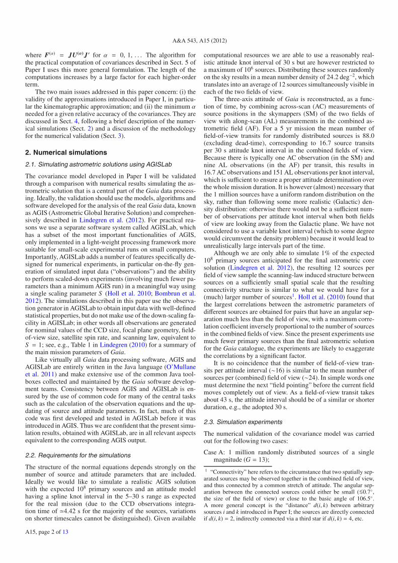
Fig. 2. Definition of the angles ψi and ψ j for two sources iand j separated by the angle θ. NCP is the North Celestial Pole(δ = +90◦).

predicted variances for some very specific combinations of theastrometric parameters of the sources. Two such quantities arethe sum and the difference of the parallaxes, Σ� ≡ �i +� j andΔ� = �i −� j. The former may be used to estimate the distanceto a binary or cluster, using the mean parallax, while the sec-ond is relevant for example for testing whether the sources arephysically connected. In both cases it is important that the vari-ance of the combination is correctly estimated. The example isparticularly interesting, since a positive correlation between theparallax errors would be detrimental for the first purpose, butbeneficial for the second (the reverse is true for negative correla-tion). Moreover, the transformation from (�i, � j) to (Σ�,Δ�)is orthogonal and therefore preserves the information in the orig-inal data. But whereas the variances of the original data donot depend on the covariance, the variances of the transformeddata do.

Extending this idea to the positions and proper motions isnot so obvious, as their errors are vector quantities in the tan-gent plane of the celestial sphere. The proposed solution is todecompose the vectorial errors into components that are paral-lel and normal to the great-circle arc connecting the two sources(Fig. 2). For convenience, we introduce a generic variable ϕ rep-resenting “differential position” in much the same way as μis used to represent “proper motion”. Thus ϕα∗ = Δα cos δand ϕδ = Δδ. The corresponding components parallel and nor-mal to the great-circle arc are denoted ϕ|| and ϕ⊥, and similarlyfor the proper motion components μ|| and μ⊥. With ψ denot-ing the position angle of the great-circle arc from i to j at therespective source, we have:

ϕ|| = ϕα∗ sinψ + ϕδ cosψϕ⊥= −ϕα∗ cosψ + ϕδ sinψμ|| = μα∗ sinψ + μδ cosψμ⊥= −μα∗ cosψ + μδ sinψ

⎫⎪⎪⎪⎪⎪⎪⎪⎬⎪⎪⎪⎪⎪⎪⎪⎭. (8)

We can now define an orthogonal transformation from the 10 as-trometric parameter errors in ei and e j to the errors in the10 quantities Σϕ||, Σϕ⊥, Σ�, Σμ||, Σμ⊥, Δϕ||, Δϕ⊥, Δ�, Δμ||,and Δμ⊥ obtained as the sums and differences of the variablesin Eq. (8). The Jacobian J i j of this transformation is detailed

Aut

ocov

aria

nce

func

tion

[μas

2 ]

−20

−10

0

10

20

30

40

50

60

70

80

90

Normalised delay τ/Δt

0 0.5 1.0 1.5 2.0 2.5 3.0 3.5 4.0 4.5 5.0 5.5 6.0 6.5 7.0

Cubic attitude splineKinematographic model (α = 4)

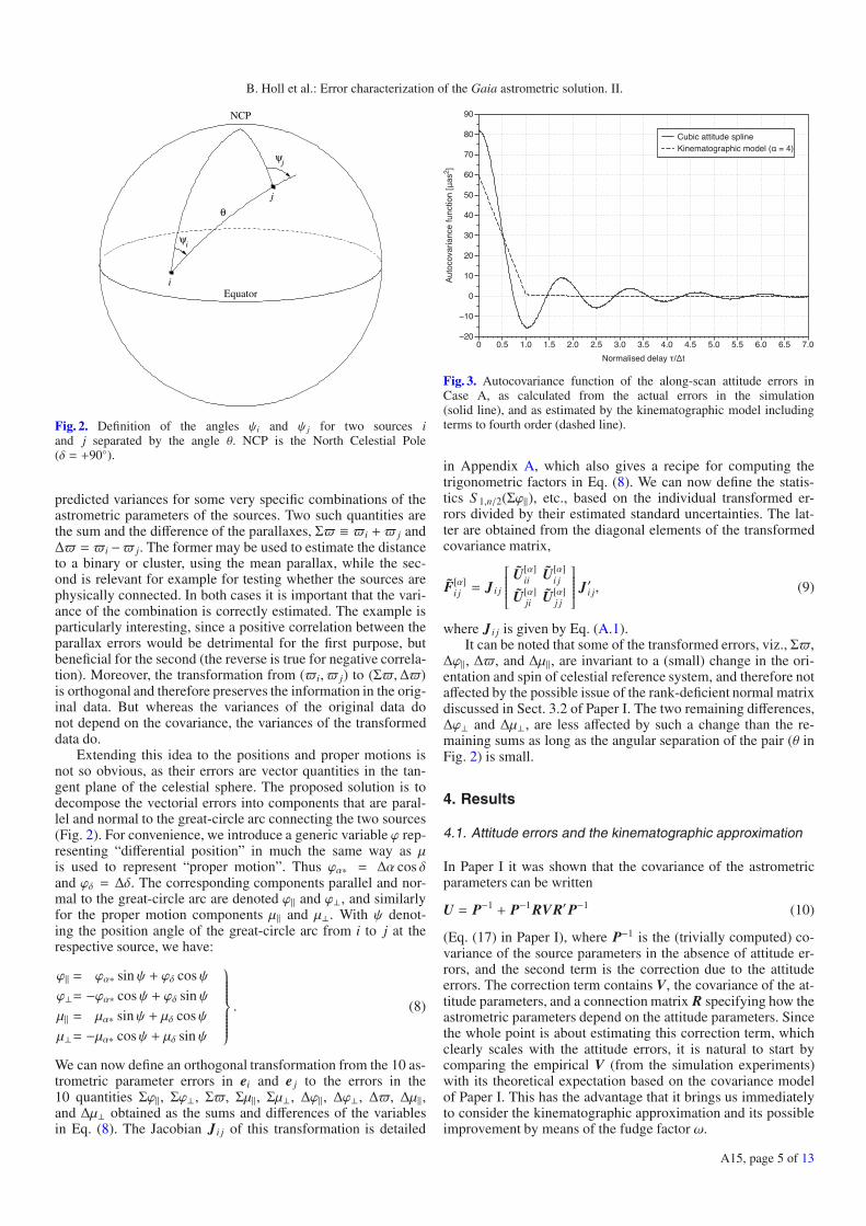
Fig. 3. Autocovariance function of the along-scan attitude errors inCase A, as calculated from the actual errors in the simulation(solid line), and as estimated by the kinematographic model includingterms to fourth order (dashed line).

in Appendix A, which also gives a recipe for computing thetrigonometric factors in Eq. (8). We can now define the statis-tics S 1,n/2(Σϕ||), etc., based on the individual transformed er-rors divided by their estimated standard uncertainties. The lat-ter are obtained from the diagonal elements of the transformedcovariance matrix,

F[α]i j = J i j

⎡⎢⎢⎢⎢⎢⎢⎣U[α]

ii U[α]i j

U[α]ji U[α]

j j

⎤⎥⎥⎥⎥⎥⎥⎦ J ′i j, (9)

where J i j is given by Eq. (A.1).It can be noted that some of the transformed errors, viz., Σ�,

Δϕ||, Δ�, and Δμ||, are invariant to a (small) change in the ori-entation and spin of celestial reference system, and therefore notaffected by the possible issue of the rank-deficient normal matrixdiscussed in Sect. 3.2 of Paper I. The two remaining differences,Δϕ⊥ and Δμ⊥, are less affected by such a change than the re-maining sums as long as the angular separation of the pair (θ inFig. 2) is small.

4. Results

4.1. Attitude errors and the kinematographic approximation

In Paper I it was shown that the covariance of the astrometricparameters can be written

U = P−1 + P−1RVR′P−1 (10)

(Eq. (17) in Paper I), where P−1 is the (trivially computed) co-variance of the source parameters in the absence of attitude er-rors, and the second term is the correction due to the attitudeerrors. The correction term contains V, the covariance of the at-titude parameters, and a connection matrix R specifying how theastrometric parameters depend on the attitude parameters. Sincethe whole point is about estimating this correction term, whichclearly scales with the attitude errors, it is natural to start bycomparing the empirical V (from the simulation experiments)with its theoretical expectation based on the covariance modelof Paper I. This has the advantage that it brings us immediatelyto consider the kinematographic approximation and its possibleimprovement by means of the fudge factor ω.

A15, page 5 of 13

A&A 543, A15 (2012)

The solid line in Fig. 3 is the autocovariance function C4(τ)of the actual along-scan attitude errors for the third (middle) yearof the simulation in Case A, computed according to Eq. (C.1) ofPaper I. The subscript 4 indicates that it is based on the attitudemodel using cubic splines (i.e., of order M = 4). On the horizon-tal axis the delay τ is expressed in units of the spline knot intervalΔt = 30 s. The dashed line is the autocovariance C1(τ) accordingto the kinematographic model for a bin width of B = 30 s, cal-culated according to Paper I by adding terms up to and includingα = 4 and putting ω = 1.

Comparing Fig. 3 with its theoretical counterpart, Fig. C.1(bottom) in Paper I, two differences stand out. First, the empiri-cal autocovariance function for the cubic attitude spline in Fig. 3goes through zero already at the delay τ = 0.74Δt, compared tothe theoretical τ = Δt expected from Fig. C.1 (Paper I). A possi-ble explanation of this result is given in Appendix D. Secondly,the variance is correspondingly larger, C4(0) � C1(0)/0.74, mak-ing the integrals of the two autocovariance functions roughlyequal (which makes sense since the integral is the inverse ofthe mean rate of the astrometric weight of the observations). InPaper I the correlation length L of the attitude autocovariancefunction was defined as the value of τ at the first zero crossing;thus we use L = 22.2 s in the following.

The autocovariance functions in Fig. 3 refer to the instan-taneous attitude errors e(t) from the simulations or accordingto theory. As explained in Appendix C of Paper I, the attitudeerror a(t) obtained by averaging e(t) over the nine consecu-tive CCD observations in the astrometric field is in fact morerelevant for the astrometric errors. In particular, we may esti-mate the fudge factor ω by comparing the variance of a(t) fromthe simulations with the variance according to the fourth-orderkinematographic approximation. The latter is calculated as

Var[a[4]]=

4∑

α=0

ωα+1Var[a(α)], (11)

where the variances on the right-hand side of the equation arecomputed as described in Paper I, using ω = 1. Adjusting ωfor equality between Var[a] from the simulation and the sum inEq. (11) gives ω = 1.158.

This empirical estimate of ω agrees very well with the theo-retical prediction from Eq. (C.5) in Paper I. Using the correlationlength L = 22.2 s from Fig. 3, the attitude bin width B = 30 s andthe temporal separation of the CCD observations, T = 4.85 s, weobtain ω = 1.164. In the subsequent analysis of the astrometricerrors we will consider the two cases ω = 1 and ω = 1.16.

4.2. Astrometric errors

The main results for the astrometric errors are summarised inTables 1–4 and discussed hereafter. It should be recalled thatthe tables give the statistic S ν,n defined by Eq. (5), which ideallyshould be zero. A value of +0.1, for example, means that the cor-responding variance is underestimated by 10%, in the sense thatit requires correction by the factor 1.1. The corresponding stan-dard uncertainty is underestimated by �5%, in that it requires acorrection by the factor

√1.1 � 1.05.

Although the astrometric errors are of course obtained forall 106 sources in each experiment, the calculation of the the-oretical covariances was for practical reasons only done for300 000 sources at each magnitude (i.e., for 300 000 sources inCase A, and for 300 000 brighter and an equal number of fainter

Num

ber

of p

airs

per

bin

0

1000

2000

3000

4000

5000

6000

Separation θ [deg]

0 0.1 0.2 0.3 0.4 0.5 0.6 0.7 0.8

Fig. 4. Distribution of the separation angle θ for the considered150 000 pairs of sources in Case A and B (G = 13).

Table 1. Single source statistics in Case A.

α = 0 α = 1 α = 2 α = 3 α = 4

ω = 1.00

S 5,n +0.0536 +0.0215 +0.0129 +0.0094 +0.0078α∗ +0.0504 +0.0184 +0.0099 +0.0065 +0.0049δ +0.0497 +0.0178 +0.0093 +0.0059 +0.0044� +0.0553 +0.0232 +0.0148 +0.0116 +0.0102μα∗ +0.0559 +0.0238 +0.0150 +0.0114 +0.0097μδ +0.0539 +0.0218 +0.0130 +0.0096 +0.0079

ω = 1.16

S 5,n +0.0536 +0.0166 +0.0051 −0.0002 −0.0030α∗ +0.0504 +0.0135 +0.0021 −0.0031 −0.0058δ +0.0497 +0.0128 +0.0015 −0.0036 −0.0063� +0.0553 +0.0183 +0.0071 +0.0022 −0.0004μα∗ +0.0559 +0.0188 +0.0071 +0.0017 −0.0013μδ +0.0539 +0.0168 +0.0052 −0.0001 −0.0030

Notes. S 5,n is the statistic testing the 5 × 5 covariance matrices ofthe n sources at different levels of approximation (α). The subsequentlines give the statistic S 1,n for the different astrometric parameters. Thenumber of sources considered is n = 3× 105 which gives an uncertaintyof ±0.0012 for S 5,n and ±0.0026 for S 1,n. Results are given for two val-ues of the fudge factor ω. The results for α = 0 are unaffected by thevalue of ω, because the attitude variance is not taken into account in thezero-order approximation.

sources in Case B). Figure 4 shows the distribution of the separa-tion angle θ for the 150 000 source pairs considered when com-puting the source pair statistics in Case A (Table 2) and for thebrighter pairs in Case B (Table 4). The distribution is essentiallythe same for the fainter pairs in Case B. The mean separationis 〈θ〉 = 0.21◦.

4.2.1. Case A (uniform brightness)

In this case we have the simplest possible configuration ofsources (uniform brightness and uniform distribution over thecelestial sphere), implying a constant astrometric weight per ob-servation, per source, and per attitude bin. The average numberof sources simultaneously visible in the combined field of viewis 24 (the actual number at any time is a Poisson random variablewith mean value 24, and consequently has a standard deviation

A15, page 6 of 13

B. Holl et al.: Error characterization of the Gaia astrometric solution. II.

Table 2. Source pair statistics in Case A.

α = 0 α = 1 α = 2 α = 3 α = 4

ω = 1.00

S 10,n/2 +0.0539 +0.0215 +0.0129 +0.0095 +0.0079Σϕ || +0.0897 +0.0332 +0.0172 +0.0108 +0.0079Σϕ⊥ +0.0909 +0.0360 +0.0202 +0.0140 +0.0111Σ� +0.0990 +0.0428 +0.0272 +0.0211 +0.0184Σμ || +0.1022 +0.0451 +0.0286 +0.0219 +0.0187Σμ⊥ +0.1025 +0.0470 +0.0308 +0.0242 +0.0211Δϕ || +0.0051 −0.0026 −0.0036 −0.0038 −0.0039Δϕ⊥ +0.0086 −0.0009 −0.0022 −0.0025 −0.0026Δ� +0.0155 +0.0068 +0.0058 +0.0055 +0.0054Δμ || +0.0078 +0.0000 −0.0010 −0.0013 −0.0014Δμ⊥ +0.0077 −0.0018 −0.0031 −0.0034 −0.0036

ω = 1.16

S 10,n/2 +0.0539 +0.0166 +0.0052 +0.0001 −0.0027Σϕ || +0.0897 +0.0247 +0.0036 −0.0060 −0.0111Σϕ⊥ +0.0909 +0.0277 +0.0070 −0.0025 −0.0075Σ� +0.0990 +0.0344 +0.0138 +0.0045 −0.0002Σμ || +0.1022 +0.0365 +0.0148 +0.0046 −0.0009Σμ⊥ +0.1025 +0.0387 +0.0173 +0.0074 +0.0019Δϕ || +0.0051 −0.0038 −0.0051 −0.0055 −0.0057Δϕ⊥ +0.0086 −0.0024 −0.0041 −0.0046 −0.0048Δ� +0.0155 +0.0055 +0.0041 +0.0036 +0.0034Δμ || +0.0078 −0.0012 −0.0026 −0.0030 −0.0032Δμ⊥ +0.0077 −0.0033 −0.0050 −0.0056 −0.0058

Notes. S 10,n/2 is the statistic testing the 10 × 10 joint covariance matri-ces of the n/2 pairs of sources. The subsequent lines give the statisticS 1,n/2 for the sums and differences of the astrometric parameters re-solved along and perpendicular to the arc joining the two sources. Sincen = 3×105 the uncertainty is ±0.0012 for S 10,n/2 and ±0.0037 for S 1,n/2.Results are given for two values of the fudge factor ω. The results forα = 0 are unaffected by the value of ω, because the attitude variance isnot taken into account in the zero-order approximation.

of nearly 5). According to Sect. 4.5 in Paper I (see also Hollet al. 2010), we thus expect that the zero-order covariance esti-mate U[0] underestimates the variances by (at least) 1/25 � 4%,and that the (neglected) correlations between sources with asmall angular separation is also of this size.

The single-source statistics S 5,n and S 1,n for Case A, givenin Table 1, show that the underestimation of the variances forα = 0 is in fact slightly worse, or about 5–6% depending onwhich parameter is considered. The smaller value is obtainedfor the declination at the mean epoch of observation, δ, and alarger value is obtained for the proper motion in right ascen-sion, μα∗. As we shall see, it is a general feature that δ is slightlyless and μα∗ slightly more susceptible to the attitude errors thanthe other astrometric parameters. This is probably related to themore favourable geometry for the determination of δ implied bythe scanning law, also reflected in the generally smaller uncer-tainties in that parameter (e.g., Eq. (5.5) and Table 3 in Lindegren2010)3.

In the higher-order approximations (α = 1, 2, . . . ) the de-gree of underestimation gradually decreases but does not disap-pear for ω = 1 (upper part of Table 1). Using the fudge factorω = 1.16 estimated from the attitude variance gives much bet-ter results and almost correct variances for α = 3. For α = 4 itgives a small overestimation of the variances (negative valuesin the table), suggesting that a slightly smaller fudge factor

3 The difference would be further accentuated in ecliptical coordinates,as the scanning law is symmetric with respect to the ecliptic.

Nor

mal

ized

freq

uenc

y

0

0.05

0.10

0.15

χ25 G-mag 13

0 2 4 6 8 10 12 14

5 dof pdfα = 0α = 1α = 2α = 3α = 4

Fig. 5. Distribution of the chi-square values included in the calcula-tion of S 5,n for the single sources in Case A. The thick grey curveis the expected chi-square distribution with 5 degrees of freedom; thecoloured curves give the experimental distribution for 300 000 sourcesusing successively higher orders of approximation (α) for the estimatedcovariances. A fudge factor ω = 1.16 was assumed. For the highest or-der (α = 4) the experimental distribution is indistinguishable from thetheoretical one.

should perhaps be preferred. Figure 5 shows that the individualsource statistics X2

i (for ν = 5) follow the expected chi-squaredistribution for α ≥ 3.

Table 2 gives the results for the source pair statistics S 10,n/2and S 1,n/2. The overall results given by S 10,n/2 are almostidentical to the S 5,n in Table 1. However, a different pictureemerges when the results are divided up between the sums (Σ)and differences (Δ) of the errors in a pair. In the zero-order ap-proximation (α = 0) the variances of the sums are strongly un-derestimated (by 9–10%), while the differences are only slightlyunderestimated (by about 1%). Compared with the single sourcestatistics in Table 1 the underestimation of the sums Σ is almostdoubled, which can be understood as the combined result ofunderestimating the variance of the parameter for each source(as in Table 1) and neglecting the positive correlation betweenthem; for the differences Δ the two effects almost cancel sincethe correlation enters with the opposite sign.

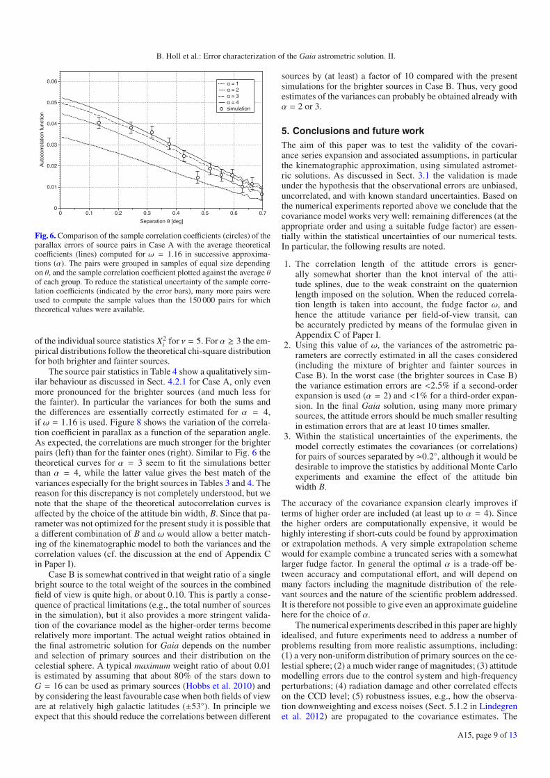
Going to higher orders (α = 1, 2, . . . ) improves the re-sults. At α = 3 and 4 and using the fudge factor ω = 1.16 theagreement is quite good in all cases considered, when the sta-tistical uncertainties are taken into account. The fact that boththe sums Σ and the differences Δ obtain virtually unbiased vari-ances indicates that the correlations at the relevant spatial scales(�0.2◦) are correctly estimated by the model. A more direct val-idation of this can be made by comparing the sample correla-tion coefficients from the simulation with the theoretical values.Figure 6 shows such a comparison for the parallaxes; the resultsfor the other astrometric parameters are very similar (cf. Hollet al. 2010). Again, the simulations suggest that, for ω = 1.16,the best agreement is found for α = 3, alternatively that a slightlysmaller value of ω should be used.

When comparing the results for the parameters that are in-variant to a change in the reference system (e.g., Σ�) to thosethat are not (the remaining Σ parameters), we do not find anydifference that could be related to the rank deficiency of the nor-mal matrix (Sect. 3.3). We conclude that the rank deficiency isnot an issue at the level of errors considered in this study.

A15, page 7 of 13

A&A 543, A15 (2012)

Table 3. Single source statistics in Case B.

G = 13 G = 15α = 0 α = 1 α = 2 α = 3 α = 4 α = 0 α = 1 α = 2 α = 3 α = 4

ω = 1.00S 5,n +0.1416 +0.0619 +0.0394 +0.0302 +0.0258 +0.0207 +0.0078 +0.0045 +0.0031 +0.0025α∗ +0.1388 +0.0593 +0.0370 +0.0279 +0.0236 +0.0189 +0.0060 +0.0028 +0.0015 +0.0008δ +0.1365 +0.0572 +0.0351 +0.0262 +0.0220 +0.0199 +0.0070 +0.0037 +0.0025 +0.0019� +0.1409 +0.0613 +0.0394 +0.0307 +0.0267 +0.0175 +0.0047 +0.0015 +0.0002 −0.0003μα∗ +0.1464 +0.0664 +0.0435 +0.0340 +0.0294 +0.0223 +0.0093 +0.0060 +0.0046 +0.0040μδ +0.1416 +0.0619 +0.0393 +0.0300 +0.0255 +0.0221 +0.0092 +0.0059 +0.0046 +0.0039

ω = 1.16S 5,n +0.1416 +0.0502 +0.0208 +0.0069 −0.0006 +0.0207 +0.0057 +0.0013 −0.0007 −0.0019α∗ +0.1388 +0.0476 +0.0184 +0.0049 −0.0025 +0.0189 +0.0040 −0.0004 −0.0024 −0.0035δ +0.1365 +0.0456 +0.0167 +0.0033 −0.0039 +0.0199 +0.0049 +0.0006 −0.0014 −0.0025� +0.1409 +0.0496 +0.0210 +0.0079 +0.0010 +0.0175 +0.0026 −0.0016 −0.0035 −0.0045μα∗ +0.1464 +0.0547 +0.0247 +0.0105 +0.0026 +0.0223 +0.0073 +0.0028 +0.0007 −0.0005μδ +0.1416 +0.0502 +0.0206 +0.0067 −0.0010 +0.0221 +0.0072 +0.0027 +0.0007 −0.0005

Notes. See Table 1 for an explanation of the different lines. The statistical uncertainty is ±0.0012 for S 5,n and ±0.0026 for S 1,n at both magnitudes.

Table 4. Source pair statistics in Case B.

G = 13 G = 15α = 0 α = 1 α = 2 α = 3 α = 4 α = 0 α = 1 α = 2 α = 3 α = 4

ω = 1.00S 10,n/2 +0.1415 +0.0599 +0.0375 +0.0285 +0.0243 +0.0213 +0.0083 +0.0050 +0.0037 +0.0031Σϕ || +0.2475 +0.1046 +0.0630 +0.0461 +0.0381 +0.0400 +0.0172 +0.0110 +0.0086 +0.0074Σϕ⊥ +0.2433 +0.1048 +0.0641 +0.0475 +0.0397 +0.0327 +0.0107 +0.0047 +0.0023 +0.0011Σ� +0.2504 +0.1092 +0.0686 +0.0523 +0.0449 +0.0362 +0.0138 +0.0078 +0.0055 +0.0044Σμ || +0.2601 +0.1158 +0.0731 +0.0554 +0.0468 +0.0350 +0.0123 +0.0061 +0.0035 +0.0022Σμ⊥ +0.2605 +0.1201 +0.0783 +0.0608 +0.0524 +0.0429 +0.0208 +0.0146 +0.0121 +0.0108Δϕ || +0.0240 +0.0048 +0.0024 +0.0017 +0.0015 +0.0034 +0.0002 −0.0001 −0.0002 −0.0003Δϕ⊥ +0.0292 +0.0054 +0.0022 +0.0013 +0.0010 +0.0004 −0.0034 −0.0039 −0.0040 −0.0041Δ� +0.0345 +0.0129 +0.0101 +0.0094 +0.0091 +0.0025 −0.0010 −0.0014 −0.0015 −0.0015Δμ || +0.0262 +0.0069 +0.0043 +0.0035 +0.0033 +0.0102 +0.0070 +0.0066 +0.0065 +0.0065Δμ⊥ +0.0300 +0.0063 +0.0029 +0.0020 +0.0016 +0.0035 −0.0003 −0.0008 −0.0010 −0.0010

ω = 1.16S 10,n/2 +0.1415 +0.0484 +0.0196 +0.0065 −0.0006 +0.0213 +0.0063 +0.0019 −0.0001 −0.0012Σϕ || +0.2475 +0.0848 +0.0315 +0.0068 −0.0065 +0.0400 +0.0136 +0.0054 +0.0016 −0.0005Σϕ⊥ +0.2433 +0.0854 +0.0333 +0.0091 −0.0040 +0.0327 +0.0073 −0.0007 −0.0045 −0.0065Σ� +0.2504 +0.0896 +0.0374 +0.0137 +0.0013 +0.0362 +0.0103 +0.0024 −0.0012 −0.0032Σμ || +0.2601 +0.0958 +0.0410 +0.0152 +0.0010 +0.0350 +0.0088 +0.0004 −0.0035 −0.0057Σμ⊥ +0.2605 +0.1005 +0.0469 +0.0214 +0.0074 +0.0429 +0.0173 +0.0091 +0.0052 +0.0030Δϕ || +0.0240 +0.0019 −0.0014 −0.0024 −0.0029 +0.0034 −0.0003 −0.0008 −0.0009 −0.0010Δϕ⊥ +0.0292 +0.0018 −0.0025 −0.0038 −0.0044 +0.0004 −0.0040 −0.0047 −0.0049 −0.0050Δ� +0.0345 +0.0095 +0.0059 +0.0047 +0.0043 +0.0025 −0.0015 −0.0021 −0.0023 −0.0023Δμ || +0.0262 +0.0039 +0.0004 −0.0007 −0.0012 +0.0102 +0.0065 +0.0060 +0.0058 +0.0057Δμ⊥ +0.0300 +0.0026 −0.0018 −0.0033 −0.0039 +0.0035 −0.0009 −0.0016 −0.0018 −0.0019

Notes. See Table 2 for an explanation of the different lines. The statistical uncertainty is ±0.0012 for S 10,n/2 and ±0.0037 for S 1,n/2 at bothmagnitudes.

4.2.2. Case B (two different magnitudes)

The total number of observations in Case B is the same as inCase A, but only 30% of them have the same noise level asbefore, σAL = 92 μas (for G = 13), while 70% have σAL =231 μas (for G = 15). The total astrometric weight is thereforeabout 41% of what we had in Case A, and the attitude varianceis expected to be about 2.4 times higher.

The single-source statistics S 5,n and S 1,n for Case B are givenin Table 3. For the brighter sources (G = 13) the underestimationof the variances for α = 0 is now about 14%, or 2.6 times higher

than in Case A, in reasonable agreement with the increased at-titude variance. For the fainter sources the underestimation isonly 2%, or 6.8 times smaller than for the brighter sources,mainly reflecting the weight ratio 6.3 between the observations.

In the higher-order approximations (α = 1, 2, . . . ) the de-gree of underestimation decreases in much the same way as inCase A, if one allows for the different overall levels among thebrighter and fainter sources. This is true for both values of thefudge factor ω. It is especially gratifying to note that the samefactor ω = 1.16 (or perhaps a slightly smaller value) turns out tobe optimal at both magnitudes. Figure 7 shows the distribution

A15, page 8 of 13

B. Holl et al.: Error characterization of the Gaia astrometric solution. II.

α = 1α = 2α = 3α = 4simulation

Aut

ocor

rela

tion

func

tion

0

0.01

0.02

0.03

0.04

0.05

0.06

Separation θ [deg]

0 0.1 0.2 0.3 0.4 0.5 0.6 0.7

Fig. 6. Comparison of the sample correlation coefficients (circles) of theparallax errors of source pairs in Case A with the average theoreticalcoefficients (lines) computed for ω = 1.16 in successive approxima-tions (α). The pairs were grouped in samples of equal size dependingon θ, and the sample correlation coefficient plotted against the average θof each group. To reduce the statistical uncertainty of the sample corre-lation coefficients (indicated by the error bars), many more pairs wereused to compute the sample values than the 150 000 pairs for whichtheoretical values were available.

of the individual source statistics X2i for ν = 5. For α ≥ 3 the em-

pirical distributions follow the theoretical chi-square distributionfor both brighter and fainter sources.

The source pair statistics in Table 4 show a qualitatively sim-ilar behaviour as discussed in Sect. 4.2.1 for Case A, only evenmore pronounced for the brighter sources (and much less forthe fainter). In particular the variances for both the sums andthe differences are essentially correctly estimated for α = 4,if ω = 1.16 is used. Figure 8 shows the variation of the correla-tion coefficient in parallax as a function of the separation angle.As expected, the correlations are much stronger for the brighterpairs (left) than for the fainter ones (right). Similar to Fig. 6 thetheoretical curves for α = 3 seem to fit the simulations betterthan α = 4, while the latter value gives the best match of thevariances especially for the bright sources in Tables 3 and 4. Thereason for this discrepancy is not completely understood, but wenote that the shape of the theoretical autocorrelation curves isaffected by the choice of the attitude bin width, B. Since that pa-rameter was not optimized for the present study it is possible thata different combination of B and ω would allow a better match-ing of the kinematographic model to both the variances and thecorrelation values (cf. the discussion at the end of Appendix Cin Paper I).

Case B is somewhat contrived in that weight ratio of a singlebright source to the total weight of the sources in the combinedfield of view is quite high, or about 0.10. This is partly a conse-quence of practical limitations (e.g., the total number of sourcesin the simulation), but it also provides a more stringent valida-tion of the covariance model as the higher-order terms becomerelatively more important. The actual weight ratios obtained inthe final astrometric solution for Gaia depends on the numberand selection of primary sources and their distribution on thecelestial sphere. A typical maximum weight ratio of about 0.01is estimated by assuming that about 80% of the stars down toG = 16 can be used as primary sources (Hobbs et al. 2010) andby considering the least favourable case when both fields of vieware at relatively high galactic latitudes (±53◦). In principle weexpect that this should reduce the correlations between different

sources by (at least) a factor of 10 compared with the presentsimulations for the brighter sources in Case B. Thus, very goodestimates of the variances can probably be obtained already withα = 2 or 3.

5. Conclusions and future workThe aim of this paper was to test the validity of the covari-ance series expansion and associated assumptions, in particularthe kinematographic approximation, using simulated astromet-ric solutions. As discussed in Sect. 3.1 the validation is madeunder the hypothesis that the observational errors are unbiased,uncorrelated, and with known standard uncertainties. Based onthe numerical experiments reported above we conclude that thecovariance model works very well: remaining differences (at theappropriate order and using a suitable fudge factor) are essen-tially within the statistical uncertainties of our numerical tests.In particular, the following results are noted.

1. The correlation length of the attitude errors is gener-ally somewhat shorter than the knot interval of the atti-tude splines, due to the weak constraint on the quaternionlength imposed on the solution. When the reduced correla-tion length is taken into account, the fudge factor ω, andhence the attitude variance per field-of-view transit, canbe accurately predicted by means of the formulae given inAppendix C of Paper I.

2. Using this value of ω, the variances of the astrometric pa-rameters are correctly estimated in all the cases considered(including the mixture of brighter and fainter sources inCase B). In the worst case (the brighter sources in Case B)the variance estimation errors are <2.5% if a second-orderexpansion is used (α = 2) and <1% for a third-order expan-sion. In the final Gaia solution, using many more primarysources, the attitude errors should be much smaller resultingin estimation errors that are at least 10 times smaller.

3. Within the statistical uncertainties of the experiments, themodel correctly estimates the covariances (or correlations)for pairs of sources separated by �0.2◦, although it would bedesirable to improve the statistics by additional Monte Carloexperiments and examine the effect of the attitude binwidth B.

The accuracy of the covariance expansion clearly improves ifterms of higher order are included (at least up to α = 4). Sincethe higher orders are computationally expensive, it would behighly interesting if short-cuts could be found by approximationor extrapolation methods. A very simple extrapolation schemewould for example combine a truncated series with a somewhatlarger fudge factor. In general the optimal α is a trade-off be-tween accuracy and computational effort, and will depend onmany factors including the magnitude distribution of the rele-vant sources and the nature of the scientific problem addressed.It is therefore not possible to give even an approximate guidelinehere for the choice of α.

The numerical experiments described in this paper are highlyidealised, and future experiments need to address a number ofproblems resulting from more realistic assumptions, including:(1) a very non-uniform distribution of primary sources on the ce-lestial sphere; (2) a much wider range of magnitudes; (3) attitudemodelling errors due to the control system and high-frequencyperturbations; (4) radiation damage and other correlated effectson the CCD level; (5) robustness issues, e.g., how the observa-tion downweighting and excess noises (Sect. 5.1.2 in Lindegrenet al. 2012) are propagated to the covariance estimates. The

A15, page 9 of 13

A&A 543, A15 (2012)N

orm

aliz

ed fr

eque

ncy

0

0.05

0.10

0.15

χ25 G-mag 13

0 2 4 6 8 10 12 14χ2

5 G-mag 150 2 4 6 8 10 12 14

5 dof pdfα = 0α = 1α = 2α = 3α = 4

Fig. 7. Same as Fig. 5 but for Case B, showing the distributions of the chi-square values included in the calculation of S 5,n for the brighter sources(G = 13) to the left and for the fainter sources (G = 15) to the right.

α = 1α = 2α = 3α = 4simulation

Aut

ocor

rela

tion

func

tion

0

0.02

0.04

0.06

0.08

0.10

0.12

Separation θ [deg]

0 0.1 0.2 0.3 0.4 0.5 0.6 0.7

α = 1α = 2α = 3α = 4simulation

Aut

ocor

rela

tion

func

tion

0

0.01

0.02

0.03

Separation θ [deg]

0 0.1 0.2 0.3 0.4 0.5 0.6 0.7

Fig. 8. Same as Fig. 6 but for Case B, showing the correlation coefficient for the brighter sources (G = 13) to the left and for the fainter sources(G = 15) to the right.

present study is therefore a first, but very important step to-wards a comprehensive modelling of the astrometric errors inthe Gaia catalogue.

Acknowledgements. B. Holl’s work was supported by the European Marie-Curieresearch training network ELSA (MRTN-CT-2006-033481). L. Lindegren andD. Hobbs gratefully acknowledge support by the Swedish National Space Board.We thank the referee for comments that helped to improve the paper.

Appendix A: The trigonometric factors in Eq. (8)

The Jacobian in Eq. (9) is

J i j =

⎡⎢⎢⎢⎢⎢⎢⎢⎢⎢⎢⎢⎢⎢⎢⎢⎢⎢⎢⎢⎢⎢⎢⎢⎢⎢⎢⎢⎢⎢⎢⎢⎢⎢⎢⎢⎢⎢⎢⎢⎢⎢⎢⎢⎢⎢⎢⎢⎢⎢⎢⎢⎣

si ci 0 0 0 s j c j 0 0 0

−ci si 0 0 0 −c j s j 0 0 0

0 0 1 0 0 0 0 1 0 0

0 0 0 si ci 0 0 0 s j c j

0 0 0 −ci si 0 0 0 −c j s j

si ci 0 0 0 −s j −c j 0 0 0

−ci si 0 0 0 c j −s j 0 0 0

0 0 1 0 0 0 0 −1 0 0

0 0 0 si ci 0 0 0 −s j −c j

0 0 0 −ci si 0 0 0 c j −s j

⎤⎥⎥⎥⎥⎥⎥⎥⎥⎥⎥⎥⎥⎥⎥⎥⎥⎥⎥⎥⎥⎥⎥⎥⎥⎥⎥⎥⎥⎥⎥⎥⎥⎥⎥⎥⎥⎥⎥⎥⎥⎥⎥⎥⎥⎥⎥⎥⎥⎥⎥⎥⎦

, (A.1)

where for conciseness we have put ci = cosψi, si = sinψi, etc.

The angles ψi and ψ j defined in Fig. 2 can be computed us-ing the equatorial normal triads [pi qi ri] and [p j q j r j] at thetwo sources (for the definition of the normal triad, see Eq. (5) inLindegren et al. 2012). With θ denoting the angle between thesources we have

ci ≡ cosψi = q′i r j/ sin θ

si ≡ sinψi = p′i r j/ sin θ

c j ≡ cosψ j = −q′jri/ sin θ

s j ≡ sinψ j = −p′jri/ sin θ

⎫⎪⎪⎪⎪⎪⎪⎪⎪⎪⎬⎪⎪⎪⎪⎪⎪⎪⎪⎪⎭

, (A.2)

where

sin θ = ||ri × r j||. (A.3)

If the position angles are needed they can be obtained as ψi =atan2(si, ci) and ψ j = atan2(s j, c j), where atan2 is the arctanfunction without quadrant ambiguity. Similarly, the angular sep-aration of the sources can be obtained as θ = atan2(sin θ, cos θ),where cos θ = r′i r j.

Appendix B: AGISLab

In this section we describe the software tool, AGISLab, usedfor the simulations. AGISLab was designed to be a lightweight

A15, page 10 of 13

B. Holl et al.: Error characterization of the Gaia astrometric solution. II.

Fig. B.1. Overview of AGISLab showing the block structure and infor-mation flow.

processing framework to allow small scale realistic experiments,controlled by a scale factor, S , and to help develop new algo-rithms which would eventually be used in the real mission dataprocessing software. AGISLab contains much of the algorith-mic functionality of AGIS but is designed to generate obser-vations on-the-fly as simulated input rather than ingesting rawdata (simulated or real) as is done in AGIS. The core algorithmsfor the source, attitude and global update blocks were devel-oped in AGISLab and are now in a common tool box calledAGISTools which allows them to be used also by the AGIS pro-cessing framework. There are currently two additional blocks inAGISLab, the calibration and velocity blocks. The calibrationblock has not been developed much but merely acts as a placeholder for future studies if needed. Calibration has largely beendeveloped in AGIS where it is essential for the reduction of realdata but has not yet been needed for our simulations. The ve-locity block has been used to develop algorithms and study theproblem of determining the barycentric velocity of Gaia usingits own observation data (Butkevich & Klioner 2008). This blockhas not yet been included in AGIS.

AGISLab provides features to generate a set of true param-eter values, including a random distribution of sources on thecelestial sphere and the true attitude (e.g., following the nom-inal Gaia scanning law), and hence the observations obtainedby adding a Gaussian random number to the computed (“True”)observation times. Similarly, true values for global, calibrationand velocity blocks can be generated. AGISLab can also gener-ate starting values for each block’s parameters that deviate fromthe true values by random and systematic offsets. The startingvalues for each block are created in dedicated generators andare then used as the “Running” values shown in Fig. B.1. Theyare updated each iteration with improved estimates. Both the“Running” and “True” parameters for each block are stored inmemory via a container and are used to generate errors plots, afeature that is very useful for analysis but will not be available inthe real mission. AGISLab generates observations in a scannerbased on information held in a satellite container, including forexample the CCD geometry and the satellite orbit. Additionally,the scanner must compute the source direction via a simple

or a full relativity model. Having generated the observations,AGISLab sets up the least-squares problem in dedicated proces-sors for each block. The least squares problem is then solved us-ing the conjugate gradient algorithm described in Bombrun et al.(2012). The process is iteratively repeated until convergence isachieved. Note that the generation of observations is only neededonce at the start and the observation noise is added on-the-flyto avoid storing two sets of data. Finally, AGISLab contains anumber of utilities to generate statistics and graphical output.

AGIS aims to make astrometric core solutions with up tosome 5 × 108 (primary) sources, based on about 4 × 1011 ob-servations, and is therefore built on a software framework spe-cially designed to handle very efficiently the corresponding largedata volumes and systems of equations. It is in practice hardlypossible to run AGIS with less than about 106 primary sources,which (just) gives a sufficient number of observations per unittime to do a successful attitude determination. For numerical ex-periments it is often desirable to use considerably less than 106

sources running in a correspondingly much shorter time, and itis an important feature of AGISLab is that it can run such scaled-down versions of AGIS. Moreover, in order to accumulate statis-tics of the astrometric errors, the small-scale runs may have tobe repeated many times with different noise realisations but oth-erwise identical conditions, which is easily done in AGISLabsince the simulation of the input data is an integrated part ofthe system.

The scaling in AGISLab uses a single parameter S such thatS = 1 leads to an astrometric solution that uses approximatelythe current Gaia design and a minimum of 106 primary sources,while S = 0.1 would only use 10% as many primary sources,etc. For S < 1 it is necessary to modify the Gaia design used inthe simulations in order to preserve certain key quantities suchas the mean number of sources in the focal plane at any time, themean number of field transits of a given source over the mission,and the mean number of observations per degree of freedom ofthe attitude model. In practice this is done by formally reduc-ing the focal length of the astrometric telescope (in order to getenough sources in the field of view at any time) and the spinrate of the satellite by the factor S 1/2, and increasing the timeinterval between attitude spline knots by the factor S −1 (to getenough observations per attitude spline knot interval). The mainconsiderations are as follows:

1. The total mission length is independent of S . Rationale: thedisentanglement of position, parallax and proper motion de-pends critically on having a mission length of at least afew years (nominally 5 yr). Thus it makes no sense to tryto save computations by reducing the mission length.

2. At any time, the expected number of sources in the fo-cal plane, n, should be independent of S (with n� 1).Rationale: Gaia can only make relative measurementsamong the sources simultaneously visible in the combinedfield of view. This depends on having a certain minimumnumber at any time.

3. The mean number m of field transits of a given source overthe mission should be independent of S . Rationale: the nom-inal scanning law is carefully tuned to give at least theminimum number of transits needed to guarantee success-ful resolution of the astrometric parameters for any source.Reducing m could result in bad solutions for at least somesources.

4. The mean number k of field-of-view transits of primarysources per attitude knot interval should be independentof S . Rationale: successful determination of the attitude

A15, page 11 of 13

A&A 543, A15 (2012)

spline coefficients requires a certain minimum number of ALand AC observations in each knot interval. Reducing k couldresult in bad attitude determination in some intervals.

Let L be the mission length, N the total number of primarysources on the sky (assumed to be uniformly distributed in a sta-tistical sense), ΦAL and ΦAC the full width of the field of viewin the AL and AC directions, Ω the satellite spin rate, and Δt themean time interval between attitude knots. Then

n =NπΦAL sin

(12ΦAC

), (B.1)

m =1πΩL sin

(12ΦAC

), (B.2)

k =NπΩΔt sin

(12ΦAC

), (B.3)

not counting dead-time. For the current Gaia design we have thenominal parameters L0 = 5 yr, ΦAL,0 = 0.708◦, ΦAC,0 = 0.691◦,and Ω0 = 60′′ s−1. Assuming N0 = 106 and Δt0 = 30 s we getn0 � 24, m0 � 88, and k0 � 17.

Now suppose we scale the problem by the factor S (<1),so that the total number of sources is N = S N0. To keep thesame n we see from Eq. (B.1) that ΦAL and/or ΦAC must beincreased. It is desirable to keep the focal-plane layout fixedby modifying both angles by the same factor, which can beachieved my changing the effective focal length F (nominalvalue F0 = 35 m). Using the small-angle approximation wefind that ΦAL,AC ∝ F−1 and consequently n ∝ NF−2. ChoosingF = S 1/2F0 therefore makes n independent of S . From Eq. (B.2)we then find that Ω = S 1/2Ω0 makes m independent of S , andfinally from Eq. (B.3) we find that Δt = S −1Δt0 makes k inde-pendent of S . We note that the angleΩΔt covered by the attitudeknot interval scales as S −1/2, thus preserving the ratio ΩΔt/ΦAL.To summarize:

N ∝ S 1, F ∝ S 1/2, ΦAL,AC ∝ S −1/2,

Ω ∝ S 1/2, Δt ∝ S −1, ΩΔt ∝ S −1/2. (B.4)

It can be noted that the AC field size is also related to the spinrate and precession rate of the spin axis (| z|) by the conditionthat there should be sufficient overlap between successive scansof the field of view. The prescription for z(t) is independent ofthe scaling factor, which is then also the case for | z|. The changein the z axis in one spin period (2π/Ω) is consequently inverselyproportional to Ω and scales as S −1/2. But ΦAC ∝ S −1/2, so therelative amount of field overlap is independent of S .

In conclusion, AGISLab is a versatile tool which allows bothfull scale solutions with at least one million sources and smallscale simulations which allow algorithms to be developed andtested easily. Except for the experiments shown in Fig. D.1 thesimulations presented in this paper did not use the scaling op-tion (i.e., S = 1 was used), as we wanted to have the maximumdegree of realism compatible with the available computing re-sources. However, the scaling did help greatly with the develop-ment and testing of the algorithms, which could be done veryefficiently with a much smaller S .

Appendix C: Implementation detailson the covariance model

This appendix provides some technical details concerning theimplementation of the covariance model used in this paper.

The set-up for the present simulations with 1 million sourcesand 5.2 million attitude bins results in the following amount ofdata needed by the model:

– for every source i the inverse Cholesky factor P−1/2i : 15 reals,

in total 1.5 × 107 reals;– for every source–attitude point combination ip with at least

one observation, the 5 × 1 array hip according to Eq. (I:54):5 reals. For an average of 88 field-of-view transits, eachtaking on average 1.4 attitude intervals, this gives in total6.1 × 108 reals;

– for every attitude point p, the inverse square root of theweight w−1/2

p : 1 real, in total 5.2 × 106 reals;– three arrays defining the structure of the connections. (a) For

every source a list of the attitude points at which it was ob-served, total: 1.2 × 108 integers. (b) For every attitude pointa list of the sources observed at that point, total: 1.2×108 in-tegers. (c) The array lookup can be done without any search-ing by creating one additional array pointing to where in thesource-ordered arrays a particular attitude point is referenced(or vice versa): 1.2 × 108 integers. From any of the three ar-rays the other two can be constructed, so only one of themneed to be persisted on disk.

Disregarding the matrix structure overhead and using 4 bytesper real or integer, the data size is 4 GigaByte (GB), in practiceneeding 8 GB when stored uncompressed on disk. Although thedata are stored in single precision (4 bytes), all computations aredone in double precision (8 bytes).

The model is initialised based on all AL observation made bythe AF and SM CCDs. The AC observations are not used in themodel as they contribute only marginally to the source parame-ters (see the discussion in Sect. 2.1 of Paper I), although they areby necessity included in the numerical experiments. Note thatthe model does not use the observations themselves, only val-ues related to the partial derivatives, weights, and the structureof the equations. The inverse Cholesky factor P−1/2

i and the ar-ray hip are initialised using the partial derivatives with respect tothe true astrometric parameters; the difference compared to usingthe final estimated parameters is negligible since the observationmodel can be considered linear within the parameter errors. Theweights used in w−1/2

p and hip are computed from the true obser-vation uncertainties. As mentioned in Sect. 2.3 their actual val-ues are irrelevant in Case A, and only their relative values matterin Case B. For the real mission the observation uncertainties willbe accurately estimated partly based on the residual statistics.

To use the model it must be loaded completely into mem-ory. For any Jacobian mapping to the source or attitude parame-ters, the model returns an estimate of the covariance matrix, cf.Eq. (3). Because the internal computation sequentially estimatesterms of increasing order, a stopping criterion might be used,but in practice terms are estimated up to a pre-defined maxi-mum order. The sequence of successive approximations can bereturned without additional computational cost. For most of thetests in this paper a trivial Jacobian is used that results in thecovariance matrix for a single source or pair of sources. Witha total of N sources (5N astrometric parameters) and P attitudepoints in the model, and considering the covariance of Q quan-tities (number of rows in the Jacobian), the model allocates twolarge arrays that store the intermediate data of G(α) (see Eq. (52)in Paper I): one source matrix of size Q × 5N when α is even,and one attitude matrix of size Q × P when α is odd. For ex-ample, requesting the covariance matrix for one source requiresQ = 5. For the experiments in this paper both matrices are of size

A15, page 12 of 13

B. Holl et al.: Error characterization of the Gaia astrometric solution. II.

�Q×40 MegaByte (MB), using double precision reals. Becausethe recursion alternates between the two matrices, the new ver-sion (of order α) may overwrite the old one (of order α − 2) inmemory.

When a quantity only combines a small number of sourcesthe source and attitude matrices will start out extremely sparsebut will get increasingly more populated towards higher terms.Numerical experiments by Holl et al. (2012a) suggest that forα ≥ 6 all sources are connected, implying that the source and at-titude matrices will be completely filled. Because the amount ofcomputations for each next term is proportional to the number ofnon-zero elements in the source or attitude matrix of the previousterm, the computation time will increase steeply with the numberof terms evaluated. Computing the next uneven term involves,for each of the Q quantities, the multiplication of the source(matrix) parameter element with hip for all attitude points p ob-served by the source, and storing the results at the correspondingpoints in the attitude matrix. The computation of the next eventerm involves the multiplication of an attitude (matrix) parame-ter element with h′ip for all sources i observed at this point, andstoring the results at the corresponding indices in the source ma-trix. This procedure can easily be multi-threaded by dividing upthe non-zero elements of the initial matrix, as long as the writ-ing to the target matrix is synchronised (e.g., because differentsources are observed in the same attitude interval). For this studywe used Q = 5 and 10 (for single sources and pairs), meaningthat the internal source and attitude matrices needed some 200and 400 MB, respectively. On our system, with two dual core2.3 GHz Intel Xeon processors, the multi-threaded runtime forcomputing the covariance of Q = 10 parameters up to fourthorder (α = 4) was about 6 s.

Appendix D: The flexibility of the attitude splines

In Sect. 4.1 it was noted that the autocovariance function of thealong-scan attitude errors, shown in Fig. 3, is compressed alongthe time axis compared with the theoretical function given inPaper I. The correlation length L, defined as the delay at thefirst zero of the autocovariance function, is found to be shorterthan the knot interval Δt, while in Fig. C.1 of Paper I we hadL = Δt. The result that L < Δt was at first very surprising to us,but we now understand that it is related to the numerical attituderepresentation, using splines for each of the four componentsof the quaternion. This model therefore has four degrees offreedom per knot interval, whereas the physical attitude onlyhas three. In the attitude updating of AGIS (and AGISLab)the solution is rendered unique by means of the regularizationparameter λ (see Eq. (81) in Lindegren et al. 2012), which gentlypushes the length of the quaternion towards 1. The numericalexperiments described in this paper use a very small degree of

λ = 0.1 λ = 0.01 λ = 0.0003

Aut

ocor

rela

tion

func

tion

−0.2

0

0.2

0.4

0.6

0.8

1.0

Normalised delay τ/Δt

0 0.5 1.0 1.5 2.0 2.5 3.0 3.5 4.0 4.5 5.0

Fig. D.1. Autocorrelation functions of the along-scan attitude errors fordifferent values of the attitude regularization parameter λ. These curveswere obtained in small-scale simulations of the astrometric solution, us-ing the AGISLab scaling parameter S = 0.012 for about 12 000 sourcesuniformly distributed over the celestial sphere.

regularization, with λ2 = 10−7, resulting in an attitude solutionwith (almost) maximum flexibility for the given knot interval,and hence the smallest correlation length (it may be significantthat we find L/Δt � 3/4, or one degree of freedom per corre-lation length). Small-scale tests with progressively larger valuesof λ indeed result in stiffer attitude solutions, as shown by the in-creasing correlation lengths in Fig. D.1; in the limit of large λ wehave L � Δt. Thus the flexibility of the attitude spline dependsnot only on the knot interval Δt but also on the regularizationparameter used in the solution.

ReferencesBombrun, A., Lindegren, L., Hobbs, D. L., et al. 2012, A&A, 538, A77Butkevich, A. G., & Klioner, S. A. 2008, in IAU Symp. 248, ed. W. J. Jin,

I. Platais, & M. A. C. Perryman, 252Hobbs, D., Holl, B., Lindegren, L., et al. 2010, in IAU Symp. 261, ed.

S. A. Klioner, P. K. Seidelmann, & M. H. Soffel, 315Holl, B., & Lindegren, L. 2012, A&A, 543, A14 (Paper I)Holl, B., Hobbs, D., & Lindegren, L. 2010, in IAU Symp. 261, ed. S. A. Klioner,

P. K. Seidelmann, & M. H. Soffel, 320Holl, B., Lindegren, L., & Hobbs, D. 2012a, in Workshop on Astrostatistics and

Data Mining in Large Astronomical Databases, La Palma, 30 May–3 June2011, ed. L. Sarro, J. De Ridder, L. Eyer, & W. O’Mullane, in press

Holl, B., Prod’homme, T., Lindegren, L., & Brown, A. 2012b, MNRAS, in pressLindegren, L. 2010, in IAU Symp. 261, ed. S. A. Klioner, P. K. Seidelmann, &

M. H. Soffel, 296Lindegren, L., Lammers, U., Hobbs, D., et al. 2012, A&A, 538, A78O’Mullane, W., Luri, X., Parsons, P., et al. 2011, Exp. Astron., 31, 243

A15, page 13 of 13