ERDC/ITL TR-08-1, User's Guide: Fracture Mechanics ... · nonlinear fracture mechanics analysis on reinforced concrete beams. The system consists of a graphic input/output interface

$Page 1: ERDC/ITL TR-08-1, User's Guide: Fracture Mechanics ... · nonlinear fracture mechanics analysis on reinforced concrete beams. The system consists of a graphic input/output interface$
ERD

C/IT

L TR

-08

-1

Computer Aided Structural Engineering

User’s Guide: Fracture Mechanics Analysis of Reinforced Concrete Beams (FMARCB)

Guillermo A. Riveros, Vellore S. Gopalaratnam, and Amos Chase

January 2008

Info

rmat

ion

Tec

hn

olog

y La

bor

ator

y

Approved for public release; distribution is unlimited.

Computer Aided Structural Engineering ERDC/ITL TR-08-1 January 2008


Guillermo A. Riveros

Information Technology Laboratory U.S. Army Engineer Research and Development Center 3909 Halls Ferry Road Vicksburg, MS 39180-6199

Vellore S. Gopalaratnam

Department of Civil and Environmental Engineering University of Missouri-Columbia Columbia, MO 65211

Amos Chase

Science Applications International Corporation 3535 Manor Drive, Suite 4 Vicksburg, MS 39180

Final report

Approved for public release; distribution is unlimited.

Prepared for U.S. Army Corps of Engineers Washington, DC 20314-1000

ii ERDC/ITL TR-08-1

Abstract: A finite element package has been developed to perform nonlinear fracture mechanics analysis on reinforced concrete beams. The system consists of a graphic input/output interface and analysis routines using finite element techniques. Fracture Mechanics Analysis of Reinforced Concrete Beams (FMARCB) is a two-dimensional finite element program with triangular, isoparametric, bar, and interface elements. The system uses the discrete crack approach with a fictitious crack model to represent tensile concrete softening; a confinement concrete model to characterize compression softening; a nonlinear bond-slip constitutive model for the bond-slip phenomenon, which is degraded when cracks form across the tensile reinforcement; and an elastic, perfectly plastic constitutive model to represent the yielding of the tensile reinforcement.

DISCLAIMER: The contents of this report are not to be used for advertising, publication, or promotional purposes. Citation of trade names does not constitute an official endorsement or approval of the use of such commercial products. All product names and trademarks cited are the property of their respective owners. The findings of this report are not to be construed as an official Department of the Army position unless so designated by other authorized documents. DESTROY THIS REPORT WHEN NO LONGER NEEDED. DO NOT RETURN IT TO THE ORIGINATOR.

ERDC/ITL TR-08-1 iii

Contents Preface..................................................................................................................................................viii

Unit Conversion Factors........................................................................................................................ix

1 Introduction..................................................................................................................................... 1 General description.................................................................................................................. 1 Finite element application to fracture mechanics.................................................................. 2

Concepts and description............................................................................................................ 2 Nonlinear finite element analysis on concrete structures......................................................... 3 Numerical characterization of the nonlinear fracture process in concrete.............................. 4 Crack concepts and numerical modeling ................................................................................... 4 Discrete crack model ................................................................................................................... 6 Smeared crack model.................................................................................................................. 7

Program significance................................................................................................................ 8 Overview ................................................................................................................................... 9

2 FMARCB Finite Element Description.........................................................................................10 Two-node bar element............................................................................................................10 Constant strain triangle .........................................................................................................11 Quadratic triangle...................................................................................................................13 Bilinear isoparametric element .............................................................................................15 Quadratic plane element .......................................................................................................16 Interface (spring link) element ..............................................................................................18

3 Automatic Mesh Generation.......................................................................................................20 Delauney refinement algorithm.............................................................................................20 Quad-morphing algorithm......................................................................................................21

Initial triangle mesh ...................................................................................................................22 Front definition ...........................................................................................................................22 Front edge classification............................................................................................................22 Front edge processing ...............................................................................................................22 Topological clean-up ..................................................................................................................24 Smoothing ..................................................................................................................................24

4 Material Properties Characterization, Softening Curves ........................................................25 Tension softening ...................................................................................................................25 Compression softening ..........................................................................................................26 Bond slip curve....................................................................................................................... 27 Degradation of bond-slip due to cracking.............................................................................28

5 FMARCB Graphical User Interface.............................................................................................30 File...........................................................................................................................................30

New .............................................................................................................................................30

iv ERDC/ITL TR-08-1

Open............................................................................................................................................31 Save ............................................................................................................................................31 Save as .......................................................................................................................................31 Print screen ................................................................................................................................31 Exit ..............................................................................................................................................31

Generate ................................................................................................................................. 31 Problem type ..............................................................................................................................32 Element type...............................................................................................................................32 Define structure geometry.........................................................................................................32 Define boundary conditions.......................................................................................................34 Material properties.....................................................................................................................39 Build initial mesh........................................................................................................................44

Execute ...................................................................................................................................45 Extrapolation of stresses ...........................................................................................................46 Run analysis ...............................................................................................................................48

Edit ..........................................................................................................................................48 View.........................................................................................................................................49

6 Example Problem .........................................................................................................................51 Introduction ............................................................................................................................ 51 Generation of initial mesh .....................................................................................................52 Program execution .................................................................................................................64 Analysis and validation of results..........................................................................................67 General observations on the crack patterns ........................................................................68

References............................................................................................................................................70

Appendix A: Output Files.....................................................................................................................73 DSP file ...................................................................................................................................73 DSS file(s) ...............................................................................................................................73 CRK file ................................................................................................................................... 74 CSE file(s)................................................................................................................................75 RSE file(s) ...............................................................................................................................75 RPT file(s)................................................................................................................................ 76

Report Documentation Page..............................................................................................................74

ERDC/ITL TR-08-1 v

Figures and Tables

Figures

Figure 1. Fictitious crack model and crack band model ........................................................................ 5 Figure 2. Idealization of a single crack on the smeared crack model .................................................. 8 Figure 3. Typical bar element. ................................................................................................................. 10 Figure 4. Typical constant strain triangle. ..............................................................................................12 Figure 5. Typical quadratic triangle......................................................................................................... 14 Figure 6. Typical four-node plane element in natural coordinates. .....................................................15 Figure 7. Typical eight-node plane element in natural coordinates..................................................... 17 Figure 8. Typical spring link element (D. Ngo and C. Scordelis)...........................................................19 Figure 9. Delauney triangles and associated Direchlet tesselations for nine generating

points .........................................................................................................................................20 Figure 10. Quad-morphing states definition..........................................................................................22 Figure 11. Steps in the process of generating a quadrilateral from front NA-NB. ...............................23 Figure 12. FMARCB softening curves.....................................................................................................25 Figure 13. Bond slip model. ....................................................................................................................28 Figure 14. FMARCB main window...........................................................................................................30 Figure 15. File options. ............................................................................................................................ 31 Figure 16. Program type option. .............................................................................................................32 Figure 17. Element Type option...............................................................................................................32 Figure 18. Define structure geometry option. .......................................................................................32 Figure 19. Line definition window...........................................................................................................33 Figure 20. Boundary of the defined beam. ...........................................................................................33 Figure 21. Line definition window specifying the rebar line.................................................................34 Figure 22. Main window showing the beam boundaries and the reinforcement. .............................34 Figure 23. Define boundary condition option........................................................................................35 Figure 24. Displacement boundary condition window. ........................................................................35 Figure 25. Main window showing displacement boundary conditions...............................................36 Figure 26. Force boundary condition option. ........................................................................................ 37 Figure 27. Force boundary condition window. ....................................................................................... 37 Figure 28. Main window showing the force boundary condition.........................................................38 Figure 29. Distributed force boundary condition window.....................................................................38 Figure 30. Main window showing the distributed boundary condition. ..............................................39 Figure 31. Material properties option.....................................................................................................39 Figure 32. Material properties window, define concrete regions option. ...........................................40 Figure 33. Material properties window, concrete properties option. .................................................. 41 Figure 34. Description of the angle of the gravity load......................................................................... 41

vi ERDC/ITL TR-08-1

Figure 35. Material properties window, reinforcement properties option. .........................................42 Figure 36. Material properties window, bond-slip properties option...................................................43 Figure 37. Material properties window, fracture properties option. ....................................................44 Figure 38. Build initial mesh option........................................................................................................44 Figure 39. Main window showing the quadrilateral mesh. ..................................................................45 Figure 40. Main menu, execute command............................................................................................45 Figure 41. Analysis options......................................................................................................................46 Figure 42. Extrapolation of stresses to nodes....................................................................................... 47 Figure 43. Menu bar, run analysis option. .............................................................................................48 Figure 44. Main menu, edit structural geometry option. .....................................................................49 Figure 45. Edit geometry window. ..........................................................................................................49 Figure 46. Main menu, view option........................................................................................................50 Figure 47. Details of beam geometry and loading configuration......................................................... 51 Figure 48. FMARCB main window. .........................................................................................................53 Figure 49. Program type option. .............................................................................................................53 Figure 50. Element type option...............................................................................................................53 Figure 51. Line definition window. ..........................................................................................................54 Figure 52. Main window showing beam boundaries and reinforcement. ..........................................54 Figure 53. Displacement boundary condition window. ........................................................................56 Figure 54. Main window showing the displacement boundary conditions. .......................................56 Figure 55. Force boundary condition window, left load........................................................................ 57 Figure 56. Main window showing the force boundary conditions for the example. ..........................58 Figure 57. Material properties window, concrete regions option.........................................................59 Figure 58. Concrete material properties window for the example. .....................................................60 Figure 59. Material properties window, reinforcement properties option. ......................................... 61 Figure 60. Material properties window, bond slip properties option...................................................62 Figure 61. Material properties window, fracture properties option.....................................................63 Figure 62. Main window showing the initial (elastic) mesh. ................................................................63 Figure 63. Main menu, execute command............................................................................................64 Figure 64. Pre-analysis constants and totals window...........................................................................64 Figure 65. Menu bar, make complete analysis option. ........................................................................64 Figure 66. First load cracking formation sequence. .............................................................................65 Figure 67. Load 2 cracking pattern.........................................................................................................66 Figure 68. Load 3 cracking pattern. .......................................................................................................66 Figure 69. Load 4 cracking pattern. .......................................................................................................66 Figure 70. Load 5 cracking pattern. .......................................................................................................67 Figure 71. Final cracking pattern. ...........................................................................................................67 Figure 72. Left and right load displacement curves.............................................................................68 Figure 73. Final cracking pattern results from the numerical model (top) and from the

experiments of Ghazavy-Khorasgany......................................................................................69

ERDC/ITL TR-08-1 vii

Tables

Table 1. Dimensional details of the reinforced concrete beams......................................................... 51 Table 2. Material properties experimentally determined by Ghazavy-Khorasgany (1994)...............52 Table 3. Vertices coordinates and weights for the example.................................................................55 Table 4. Load magnitudes for the example. .......................................................................................... 57 Table 5. Numerical model parameters for the example.......................................................................58

viii ERDC/ITL TR-08-1

Preface

This report presents the user’s manual for the FMARCB computer program, which is used to perform non-linear fracture mechanics analysis on reinforced concrete beams. Funding for the development of this program and preparation of this report was provided by the Computer Aided Structural Engineering program (CASE).

The computer program and report were accomplished under the general supervision of Chris Merrill, Chief, Computational Science and Engineering Branch; Dr. Cary Butler, Acting Chief, Engineering and Informatics System Division; and Dr. Deborah Dent, Acting Director, Information Technology Laboratory (ITL). This report and computer program were prepared by Dr. Guillermo A. Riveros, Engineering and Informatics Systems Division, ITL; Dr. Vellore S. Gopalaratnam, Professor, University of Missouri-Columbia; and Amos Chase, Science Applications International Corporation.

The Commander and Executive Director of ERDC is COL Richard B. Jenkins. The Director is Dr. James R. Houston.

ERDC/ITL TR-08-1 ix

Unit Conversion Factors

Multiply By To Obtain

inches 0.0254 meters

pounds (force) 4.448222 newtons

pounds (force) per inch 175.1268 newtons per meter

pounds (force) per square inch 6.894757 kilopascals

ERDC/ITL TR-08-1 1

1 Introduction

General description

A finite element package has been developed to perform nonlinear fracture mechanics analysis on reinforced concrete beams. The system consists of a graphic input/output interface and analysis routines using finite element techniques. Fracture Mechanics Analysis of Reinforced Concrete Beams (FMARCB) is a two-dimensional finite element program with triangular (three and six nodes), isoparametric (four and eight nodes), bar (truss), and interface (bond-link) elements. The system uses the discrete crack approach with the fictitious crack model (FCM) (Hillerborg et al. 1976, Hillerborg 1983, Bazant 1985, 1992) to represent tensile concrete softening; a confinement concrete model (Shah et al. 1983) to characterize compression softening; a nonlinear bond-slip constitutive model for the bond-slip phenomenon, which is degraded when cracks form across the tensile reinforcement (Hayashi and Kokusho 1986, CEB-FIP 1990); and an elastic, perfectly plastic constitutive model to represent the yielding of the tensile reinforcement.

FMARCB incorporates the Delaunay refinement algorithm (Ruppert 1995) to create a triangular topology that is then transformed into a quadrilateral mesh by the quad-morphing algorithm (Owen at al. 1999). The Delaunay refinement mesh-generation algorithm constructs meshes of triangular elements. The algorithm operates by imposing a Delaunay or constrained Delaunay triangulation that is refined by inserting additional vertices until the mesh meets constraints on element quality and size. These algorithms simultaneously offer theoretical bounds on element quality, edge lengths, and spatial grading of element sizes. They also possess the ability to triangulate general straight-line domains.

Quad-morphing (Owen at al. 1999) is a relatively new technique used for generating quadrilaterals from an existing triangle mesh. Beginning with an initial triangulation, triangles are systematically transformed and combined. Quad-morphing can be categorized as an unstructured, indirect method that utilizes an advancing front algorithm to form an all-quad mesh. As an indirect method, it is able to take advantage of local topology information from the initial triangulation. Unlike other indirect methods,

2 ERDC/ITL TR-08-1

it is able to generate boundary-sensitive rows of elements with few irregular nodes.

Finite element application to fracture mechanics

Since Hillerborg and his colleagues (Hillerborg et al. 1976) introduced the Dugdale-Barrenblatt-type model in 1976 to represent the fracture process zone in concrete, many investigators have attempted to define suitable forms for that and other types of models (Vecchio and Collins 1986). Those investigations involved both extensive experimental and numerical studies on the formation and propagation of the fracture process zone (FPZ) in concrete.

The finite element technique has the potential to play an increasingly important role in all areas of reinforced concrete research, design, and analysis. The derivations of a realistic analytical model of concrete behavior and its implementation in nonlinear finite element analysis have long been a major subject of investigation.

Concepts and description

A significant number of models and computer codes using finite element analysis have been developed to analyze nonlinear fracture mechanics in concrete structures more accurately. The complexities of developing an analytical model for reinforced concrete are:

• The structural system is three-dimensional and is composed of two materials, concrete and steel;

• The structural system has a continuously changing character because of the cracking of the concrete under increasing load;

• The effects of dowel action in the steel reinforcement bond between the steel reinforcement and the concrete and bond slip are difficult to incorporate into a general analytical model;

• The stress-strain relationship for concrete is nonlinear and is a function of many variables; and

• Concrete deformations are influenced by creep and shrinkage and are time-dependent.

Ngo and Scordelis (1967) defined finite element analysis as a general method of structural analysis in which a continuous solid is replaced by a finite number of elements interconnected by a finite number of nodal

ERDC/ITL TR-08-1 3

points. Using that, a problem in solid mechanics is transformed into a related problem of an articulated structure, which can be analyzed by the standard methods of structural analysis. The key steps that influence the accuracy of the finite element analysis are the determination of the finite element matrix and the complexity of the structural mesh used.

Nonlinear finite element analysis on concrete structures

The development of methods and models to predict and analyze the nonlinearity of mechanical behavior or the inelasticity of some materials has been an important goal. The effort to find these methods and models has resulted in the development of nonlinear finite element analysis (NLFEA) systems. These NLFEA systems have rarely been used. (The development of successful predictions of the behavior of particular structural configurations do not necessary imply its use.)

Most NLFEA systems are based on standard numerical computer-based techniques. Significant differences always remain, mostly related to the analytical description of the various features of concrete behavior, such as the cracking process, strength, and deformation characteristics (Van Den Berg 1962a,b,and c). The successful application of nonlinear finite element systems to concrete structural forms predominantly depends on realistic descriptions of material characteristics, such as failure criteria and deformational properties of concrete and steel and fracture processes of concrete and concrete-steel iteration. Incorporating such material descriptions into an existing linear-solution finite element programs led to the development of a nonlinear finite element system suitable for plane stress and asymmetric analyses, which yielded realistic predictions of behavior for a wide range of plain and reinforced concrete structural configurations.

Chang et al. (1987) showed a complete, time-independent constitutive relation for the nonlinear analysis of reinforced concrete structures. The relation consists of an improved concrete plasticity model, a multiaxial fracture criterion for concrete, a smeared model for concrete cracking, and modeling of post-fracturing behavior via tension stiffening and shear retention effects.

They stated that to consider the combined effect of steel and concrete, a smeared approach or an embedded model may be utilized to evaluate the stiffnesses of steel rebars and concrete in finite element calculations.

4 ERDC/ITL TR-08-1

Using NLFEA in fracture mechanics, an analytical model for studying the behavior of the structure over the entire range of loading can be developed. Considering all the factors mentioned earlier, better and more accurate data from the analysis of reinforced concrete are obtained for the nonlinear range using finite element analysis.

Numerical characterization of the nonlinear fracture process in concrete

Gopalaratnam and Ye (1991) reported that the numerical formulation for nonlinear fracture processes offers a simple alternative for studying the growth and development of the fracture process zone. Load-deformation characteristics as well as energy absorption history can be generated for stable fracture using an incremental crack tip advance algorithm. The process zone appears to reach a steady state length that depends on both specimen size and test configuration. At peaks loads, the process zone size was observed to be approximately 70 percent of its steady state for the range of material parameters, specimen sizes, and specimen geometries investigated. On further crack growth, the process zone size diminished gradually because of a combination of edge effects and compressive stress fields that restrained its free growth (Gopalaratman and Ye 1991).

Crack concepts and numerical modeling

The numerical aspects related to the representation of cracking have a significant influence on the NLFEA predictions. The cracking representation is based on the smeared crack approach and the use of realistic criteria for the onset of cracking and local material failure (Van Den Berg 1962a,b, c). The smeared crack approach spreads the effect of the crack over the area of an element, which corresponds to one integration Gauss point (i.e., over one quarter of the eight-node isoparametric element representing concrete). After cracking has occurred at a given Gauss point, the orientation of the principal stresses does not coincide with the orientation of the existing crack (Van Den Berg 1962a,b, c). As a result, there may be some transfer of force across the crack surfaces.

The complexity of the finite element analysis depends on whether or not the crack path is assumed in advance (Zhang and Gjorv 1991). If the crack path is assumed in advance, the finite element mesh is arranged in such a way that the crack follows either along the element boundaries or inside the elements parallel to the element boundaries. In the former case, the

ERDC/ITL TR-08-1 5

fracture zone is modeled as a separation of the element along the crack path. This is a pure crack model, often referred to as the fictitious crack model. In the latter case, the fracture zone is modeled as a change in stiffness of a row of elements along the crack path. This is referred as the crack band model (Zhang and Gjory 1991).

Figure 1 shows an application of the discrete crack approach of finite element analysis to the fictitious crack model and the crack band model. Figure 1a illustrates the separation of elements with the introduction of

Figure 1. Fictitious crack model (a) and crack band model (b). [From Hillerborg and Rots (1989).]

6 ERDC/ITL TR-08-1

closing stresses, which depend on the fracture zone deformation, w, which is equal to the node separation distance. Figure 1b illustrates the change of stiffness of a row of elements (Zhang and Gjory 1991). These two models mainly differ in the finite element formulation, but the numerical results are practically identical.

Discrete crack model

The discrete crack approach models a crack by means of a separation between element edges (Zsutty 1968). This implies a continuous change in nodal connectivity and constrains the crack to follow a path along the element edges. For general purposes, this model is not attractive, but a number of special purposes exist for which the drawbacks can be circumvented. For comparative studies and for engineering problems where a mechanism of discrete cracks is imagined in a fashion similar to a yield line mechanism, this model is effective. For such problems, one may predefine interface elements in the original mesh, keeping the topology preserved. The initial stiffness of the elements is assigned a large dummy value in order to simulate the uncracked state with rigid connection between overlapping nodes (Zsutty 1968). Upon violating a condition of crack initiation, the element stiffness is changed, and a constitutive model for discrete cracks is mobilized.

The viewpoint of the discrete crack model is still macroscopic in principle, with the basic behavior characteristics lumped into the elements. With the cracking passing along the element boundaries, the use of simple elements, such as the constant strain triangle (CST) element, is recommended for both the concept and the application (Nilson 1968).

Nilson modified this approach to allow the finite element model to generate the location of the cracks (Nilson 1968). With this representation, cracking based on the average stress exceeds the tensile strength of the concrete for the flexural problems, and the elements are disconnected at their common corners. For cracks at the exterior of the beam, the outside node is separated. For cracks at the interior of the beam, both nodal points are separated. This refined method of representing discrete cracks was further improved and partially automated by (Mufti et al. 1970). He incorporated a predefined crack using two nodes at one point connected by a linkage element. When the stresses in the elements exceed the cracking strength of the concrete, the linkage element is softened to allow the crack to open (Nilson 1968).

ERDC/ITL TR-08-1 7

The use of discrete cracking representation has received only limited acceptance because of the difficulty involved in providing an economical redefinition of the structural topology following the formation of cracks (Nilson 1968). For those problems in which dowel forces are important, discrete cracking appears to be a natural tool. Overall, in those cases in which local material behavior at a particular stage during the life of reinforcement concrete structures is of interest, a discrete cracking model is likely to be the representation of choice and is especially useful for investigating the stresses in a structural member with a known crack location (Nilson 1968).

Riveros and Gopalaratman (Riveros 2005, Riveros and Gopalaratman 2007) developed algorithms to overcome the drawbacks of discrete crack models. They allow the generation and re-meshing of multiple cracks while studying shear strength and size effects on reinforced concrete deep beams.

Smeared crack model

The counterpart of the discrete crack concept is the smeared crack concept, in which a cracked solid is imagined to be a continuum with the notion of stress and strain. The necessity for a cracking model that offers automatic generation of cracks without the redefinition of the finite element topology and completes generality in possible crack direction has led a vast majority of investigators to adopt the smeared cracking model (Nilson 1968). This procedure was introduced by Rashid (1968). He represents cracked concrete as an orthotropic material. After cracking has occurred, the modulus of elasticity of the material is reduced to zero, perpendicular to the principal tensile stress direction.

Rather than representing a single crack, this procedure has the effect of representing many finely spaced (or smeared) cracks perpendicular to the principal stress direction (Figure 2).

The smeared cracks concept can be catalogued into fixed and rotating smeared crack concepts. The smeared cracks concept uses a fixed orientation of the crack during the entire computational process, whereas a rotating concept allows the orientation of the crack to rotate with the axes of principal strain (Zwoyer and Siess 1954). Many comparatives studies in this area have been devoted towards distributed fracture. The studies revealed the danger of fixed cracks with significant shear retention.

8 ERDC/ITL TR-08-1

Figure 2. Idealization of a single crack on the smeared crack model. [From Isenberg (1991).]

Such models easily produce an over-stiff response because the local stresses that rebuild in inclined directions lead to very severe stress-locking on a global level. Basically, the shear retention factor should be taken to be as low as possible, preferably as zero, to improve the fixed smeared crack results. Studies with fixed multi-directional cracks did not have significant improvements.

It has been demonstrated that even the best possible smeared crack is not free from stress-locking because of the assumption of displacement continuity and the realism of a geometrical discontinuity. Another difficulty of this model is the danger of spurious mechanisms. These may hamper convergence and blow up the entire iterative procedure. The discrete model does not suffer from these phenomena.

Program significance

The main relevance of this computer program lies in the implantation of nonlinear fracture mechanic models with finite element methods that include the main non-linearities found in reinforced concrete beams. Concrete softening in tension and compression, bond slip, and yielding of reinforcement are the main non-linearities. These four non-linearities are the ones that provide the overall strength of the beams and are essential

ERDC/ITL TR-08-1 9

for predicting the ultimate capacity of the members. Furthermore, FMARCB incorporates automated crack initiation and propagation algorithms that combine with automated re-meshing techniques to make the discrete crack approach the way to determine the ultimate capacity of any reinforced concrete beam.

Overview

Chapter 2 includes a detailed explanation of the finite elements used in FMARCB. Chapter 3 includes a detailed explanation of the algorithms developed to perform the automatic mesh generation. The material properties characterizations are presented in Chapter 4. The graphical user interface (GUI) is described in Chapter 5, and a complete example is presented in Chapter 6.

10 ERDC/ITL TR-08-1

2 FMARCB Finite Element Description

Two-node bar element

The bar element is the simplest finite element, and it is used as a truss element with rigidity only in the axial direction. Because of this, the bar element has only two degrees of freedom (d.o.f.), one in each node, and its stiffness is a function of its area, elastic modulus, and length. Figure 3 shows a typical bar element inclined with respect to the global coordinate system.

Figure 3. Typical bar element.

The shape functions (Ni) of this element are functions of its length (L) and have the form

−

= =1 2L x xN N

L L (1)

In this case, the matrix of the derivatives of the shape functions [B] is defined as

[ ] ∂= = −⎡ ⎤⎣ ⎦∂

i

i

11 1

NBx L

(2)

ERDC/ITL TR-08-1 11

The stiffness matrix (k) is easily written as

[ ] [ ] [ ]= ∫0

L

Tk B AE B dx (3)

[ ] [ ]− −⎡ ⎤ ⎡

= − =⎡ ⎤⎤

⎢ ⎥ ⎢⎣ ⎦ − ⎥⎣ ⎦ ⎣2 2

1 11 11 1

1 1TB B

L L ⎦

1

1 (4)

[ ] [ ] [ ]−⎡ ⎤

= = ⎢ ⎥−⎣ ⎦∫0

1 1'

1 1

LT AEk B AE B dx

L (5)

in which A is the cross-sectional area and E is the modulus of elasticity. A transformation matrix [T] is required to transform the local stiffness matrix [k’] from a local coordinate system to a global coordinate system:

[ ] [ ] [ ][ ]

⎡ ⎤θ θ θ − θ − θ θ⎢ ⎥⎢ ⎥θ θ θ − θ θ − θ

= = ⎢ ⎥− θ − θ θ θ θ θ⎢ ⎥

⎢ ⎥− θ θ − θ θ θ θ⎢ ⎥⎣ ⎦

2 2

2 2

2 2

2 2

cos cos sin cos cos sin

sin cos sin sin cos sin'

cos cos sin cos cos sin

sin cos sin sin cos sin

T AEK T k TL

(6)

This element is intended to be used in conjunction with the plane elements to model steel reinforcement.

Constant strain triangle

The three-node triangle, also called the constant strain triangle, is the simplest plane element that has been incorporated into the FMARCB program. This triangle has three nodes at the side edges and two d.o.f. per node. Because of its simplicity, the integration of the shape functions to obtain the stiffness matrix is exact. This makes the analytical process easier; however, more elements will be required to obtain an acceptable solution. Since the shape functions are linear, the results of the nodal displacements will also be linear, so the stresses and strains are constant across all surfaces of the element. This characteristic of the element creates areas with the same stress values, which is a weak approximation of the real behavior of typical structures. This error is diminished with finer meshes, but this implies an increase in the number of d.o.f. of the problem, which will increase the computational effort. However, the

12 ERDC/ITL TR-08-1

results are good enough for comparison and first trial analysis. With more refined meshes, the results can be used for a complete analysis. Figure 4 shows a typical constant strain triangle.

Figure 4. Typical constant strain triangle.

The shape functions matrix is

[ ]ξ ξ ξ⎡ ⎤

= ⎢ ⎥ξ ξ ξ⎣ ⎦

1 2 3

1 2

0 0 0

0 0 0N

3 (7)

For triangles, the natural coordinates are defined as area coordinates of the type ξn. These area coordinates are ratios of area given by

ξ = ξ = ξ =1 21 2 3

A AA A

3AA

(8)

where A1, A2, and A3 are sub-areas created by a division of the triangle by an arbitrary point in the surface. For a straight-sided triangle, it has been found that the derivatives of these area coordinates give the next expressions:

∂ξ ∂ξ ∂ξ

= =∂ ∂ ∂

1 23 2 31 3 1

2 2 2y y

= 2yx A x A x A

(9)

ERDC/ITL TR-08-1 13

∂ξ ∂ξ ∂ξ

= =∂ ∂ ∂

1 32 2 13 3 2

2 2= 1

2x x x

y A y A y A (10)

where and . ij i jx x x= − ij i jy y y= −

Then the derivative of the shape function matrix is given by

[ ]⎡ ⎤⎢ ⎥= ⎢ ⎥⎢ ⎥⎣ ⎦

23 31 12

32 13 21

32 23 13 31 21 12

0 0 01

0 0 02

y y yB x x

Ax y x y x y

x (11)

If the elastic modulus matrix [E] and the thickness are constant across the element, the stiffness matrix is given by

(12) [ ] [ ] [ ][ ]= Tk tA B E B

Quadratic triangle

The quadratic triangle is a plane finite element like the constant strain triangle; however, it has six nodes, N (three at the edges and three at the element sides). This triangle has a total of 12 d.o.f. The major difference from the constant strain triangle is the grade of the shape functions. The shape functions are quadratic and are based on area coordinates. Figure 5 shows a typical quadratic triangle.

The interpolation functions are given by

( ) ( ) ( )= ξ − ξ = ξ − ξ = ξ − ξ

= ξ ξ = ξ ξ = ξ ξ1 1 1 2 2 2 3 3

4 1 2 5 2 3 6 1 3

2 1 2 1 2 1

4 4 4

N N NN N N

3 (13)

The area coordinates are not independent and have to satisfy the con-straint relation ξ1 + ξ2 + ξ3 = 1. Since we are using natural coordinates and the matrix [B] is the derivative of the shape functions but evaluated in nodal coordinates, the expression for [B] is given by [B] = [J]-1 [DN]. The [DN] matrix contains the derivative of the shape functions in natural coor-dinates and the inverse of the Jacobian Matrix [J]-1, which includes the transformation from natural coordinates to nodal coordinates by the expression:

14 ERDC/ITL TR-08-1

Figure 5. Typical quadratic triangle.

[ ] [ ]

⎡ ⎤⎢ ⎥⎢ ⎥⎢ ⎥

= ⎢ ⎥⎢ ⎥⎢ ⎥⎢ ⎥⎢ ⎥⎣ ⎦

1 1

2 2

3 3

4 4

5 5

6 6

N

x yx yx y

J Dx yx yx y

(14)

where

[ ] ( )( )

ξ − − ξ + ξ − ξ ξ −ξ⎡ ⎤= ⎢ ⎥ξ − − ξ + ξ ξ −ξ − ξ⎣ ⎦

1 3 2 2

2 3 1 3 2 1

4 1 0 4 1 4 4 4

0 4 1 4 1 4 4 4ND 3 1 (15)

Using the previous expressions, the stiffness matrix is given by the equation

[ ] [ ] [ ]= ∫T

A

k B k B t dA (16)

where the t is the element thickness, A is the area of the triangle, and [B] is function of the area coordinates ξ1, ξ2, and ξ3. The area integration of these types of elements can be evaluated in exact form if the sides are straight

ERDC/ITL TR-08-1 15

and the side nodes are in the middle. The integral can also be evaluated by the use of numerical integration with the implementation of the Gauss Quadrature.

Bilinear isoparametric element

The bilinear isoparametric element has four nodes at the edges of the element and two d.o.f. per node (Figure 6). Its shape functions are functions of natural coordinates (ξ,η). The shape functions for this element are given by the expressions:

Figure 6. Typical four-node plane element in natural coordinates.

( )( ) ( )( )( )( ) ( )(

= − ξ −η = + ξ −η

= + ξ + η = − ξ + η

1 11 24 4

1 13 44 4

1 1 1 1

1 1 1 1

N N

N N ) (17)

The process of obtaining the matrix [B] is similar to the quadratic triangle and is given by the equations

[ ] [ ]

⎡ ⎤⎢ ⎥⎢ ⎥=⎢ ⎥⎢ ⎥⎣ ⎦

1 1

2 2

3 3

4 4

N

x yx y

J Dx yx y

(18)

16 ERDC/ITL TR-08-1

[ ] ( ) ( ) ( ) ( )( ) ( ) ( ) ( )

− −η −η +η − +η⎡ ⎤= ⎢ ⎥− −ξ − + ξ + ξ −ξ⎣ ⎦

1 1 1 111 1 1 14ND (19)

(20) [ ] [ ] [ ]−= 1NB J D

The major difference in the process of obtaining the stiffness matrix from the one for the quadratic triangle is the double integration needed to obtain the stiffness matrix [k]. The equation has the form

(21) [ ] [ ] [ ][ ] [ ] [ ][ ]− −

= =∫∫ ∫ ∫1 1

1 1

T Tk B E B t dx dy B E B tJ d ξ ηd

Quadratic plane element

The quadratic plane element is similar to the four-node element, with the main differences being that it has nodes at the sides of the element and its shape functions are quadratic. This element has a total of 16 d.o.f. (two per node). It is often called the serendipity element. The process of obtaining and evaluating the stiffness matrix is identical to the previous element. The difference lies in the size of the matrices and in the shape functions (Figure 7).

ERDC/ITL TR-08-1 17

Figure 7. Typical eight-node plane element in natural coordinates.

The shape functions for this element are:

( )( ) ( ) ( )( )

( )( ) ( ) ( )( )( )( ) ( ) ( )( )

( )( ) ( ) ( )( )

= − ξ −η − − = −ξ −η

= + ξ −η − − = + ξ −η

= + ξ +η − − = + ξ +η

= −ξ +η − − = −ξ +η

21 1 11 8 5 54 2 2

21 1 12 5 6 64 2 2

21 1 13 6 7 74 2 2

21 1 14 7 8 84 2 2

1 1 1 1

1 1 1 1

1 1 1 1

1 1 1 1

N N N N

N N N N

N N N N

N N N N

(22)

[ ] [ ]

⎡ ⎤⎢ ⎥⎢ ⎥⎢ ⎥⎢ ⎥⎢ ⎥= ⎢ ⎥⎢ ⎥⎢ ⎥⎢ ⎥⎢ ⎥⎢ ⎥⎣ ⎦

1 1

2 2

3 3

4 4

5 5

6 6

7 7

8 8

N

x yx yx yx y

J Dx yx yx yx y

(23)

18 ERDC/ITL TR-08-1

[ ]

∂ ∂ ∂ ∂ ∂ ∂ ∂ ∂⎡ ⎤⎢ ⎥∂ξ ∂ξ ∂ξ ∂ξ ∂ξ ∂ξ ∂ξ ∂ξ⎢ ⎥=∂ ∂ ∂ ∂ ∂ ∂ ∂ ∂⎢ ⎥⎢ ⎥∂η ∂η ∂η ∂η ∂η ∂η ∂η ∂η⎣ ⎦

1 2 3 4 5 6 7 8

1 2 3 4 5 6 7 8

14N

N N N N N N N N

DN N N N N N N N

(24)

The way to obtain the stiffness matrix and its evaluation is the same as for the four-node isoparametric element.

Interface (spring link) element

To model the tensile softening and bond-slip conditions, the bond-link element (Ngo and Scordelis 1967) was implemented in FMARCB (Figure 8). Stresses generated between any two surfaces (steel and concrete as in bond-slip relations or concrete to concrete as in softening responses) are calculated as a function of the relative displacements between the surfaces. This type of element relies on a normal and shear stiffness to simulate the strength between the two surfaces. The stiffness matrix of the spring link element, K, is

(25) [ ] [ ] [ ][ ]= TK A C A

where

[ ]− θ − θ θ θ⎡ ⎤

= ⎢ ⎥θ − θ − θ θ⎣ ⎦

cos sin cos sin

sin cos sin cosA (26)

[ ] ⎡ ⎤= ⎢ ⎥⎣ ⎦

0

0h

v

KC

K (27)

where Kh and Kv are the stiffnesses of the longitudinal and transverse springs, respectively.

ERDC/ITL TR-08-1 19

Figure 8. Typical spring link element (D. Ngo and C. Scordelis).

20 ERDC/ITL TR-08-1

3 Automatic Mesh Generation

Delauney refinement algorithm

The Delauney triangulation splits the plane into a number of polygonal regions called tiles. Each tile has one sample point in its interior called a generating point. All other points inside the polygonal tile are closer to the generating point than to any other. The Delauney triangulation is created by connecting all generating points that share a common tile edge. Thus formed, the triangle edges are perpendicular bisectors of the tile edges.

Such a triangulation has many desirable features. It can be shown that a convex equilateral formed by two adjacent triangles has a greater minimum internal angle than if the equilateral were formed another way. In this sense, the triangles are as equilateral as possible, while thin, wedge-shaped triangles are avoided (Figure 9).

Figure 9. Delauney triangles (thin lines) and associated Direchlet tesselations (thick lines) for nine generating points. The triangle edges are perpendicular bisectors of the tile edges. The points within a tile are closer to the tile’s generating point than to any other generating point.

ERDC/ITL TR-08-1 21

The triangulation is unique (independent of the order in which the sample points are ordered) for all but trivial cases. One such case is if four points lie on the corners of a rectangle; then they may be triangulated in one of two ways. These situations occur rarely in real data, but if uniqueness is important, then a straightforward solution is to perturb one or more of the vertices on the offending rectangle.

One situation where many other techniques perform poorly is when there is a mixture of regions of high- and low-density sampling. Triangulation-based methods honor this situation by giving a large number of triangles (and hence more detail) to the highly sampled regions and large triangles (less detail) to the regions with a few samples.

Discontinuities are handled quite naturally. The surface can have a discontinuity as narrow as the sampling process permits; it simply results in near-vertical triangular facets. Note, however, that unless special action is taken, there cannot be two samples at precisely the same point on the sample plane but with different heights. This can occur with discrete digitizers when digitizing near discontinuities. A perturbation of the sample point in the correct direction is usually a satisfactory solution to this problem.

An algorithm to implement triangulation can be quite efficient and thus suitable for areas with a large number of samples. Furthermore, if further samples are obtained at a later date, they can be added to the existing triangulation without having to triangulate all the samples plus the extra samples. This makes it possible to efficiently perform a successive refinement on those areas where more detailed information is required.

Quad-morphing algorithm

Quad-morphing is a new technique used to generate quadrilaterals from an existing triangle mesh. Beginning with an initial triangulation, triangles are systematically transformed and combined. An advancing front method is used to determine the order of transformations. An all-quadrilateral mesh containing elements aligned with the area boundaries with few irregular internal nodes can be generated.

Quad-morphing is briefly outlined in the following steps (Owen at al. 1999).

22 ERDC/ITL TR-08-1

Initial triangle mesh

The surface is first triangulated. This may be done using any surface triangulation method. The local sizing for the final quadrilateral mesh will roughly follow that of the triangle mesh.

Front definition

The initial front is defined from the initial triangle mesh. Any edge in the triangulation that is adjacent to only one triangle becomes part of the initial front.

Front edge classification

Each edge in the front is initially sorted according to its state. The state of a front edge defines how the edge will eventually be used in forming a quadrilateral. Angles between adjacent front edges determine the state of an individual front. Front edges will be updated and reshuffled as the algorithm proceeds. Figure 10 shows the four possible states of a front, with the front edge indicated by the bold line.

State 1-0 State 0-1 State 1-1 State 0-0

Figure 10. Quad-morphing states definition.

Front edge processing

Each front edge is individually processed to create a new quadrilateral from the triangles in the initial mesh. Figure 11 shows front NA-NB in the triangulation ready to be processed. Front edges are handled differently according to their current state classification. As quadrilaterals are formed, the front is redefined and adjacent front edge states are updated. The current front always defines the interface between quadrilateral elements in the final mesh and triangle elements in the initial triangle mesh. This process can be further subdivided into the following sub-steps.

ERDC/ITL TR-08-1 23

Figure 11. Steps in the process of generating a quadrilateral from front NA-NB.

Check for special cases

Before constructing a quadrilateral from the current front, several special case scenarios are checked. These include situations where large transitions or small angles exist local to the front. In these cases, a seam or transition seam operation is performed.

Side edge definition

Using the front edge as the initial base edge of the quadrilateral, side edges are defined. Side edges may be defined by using an existing edge in the initial triangle mesh, by swapping the diagonal of adjacent triangles, or by splitting triangles to create a new edge. In Figure 11b, side edge NB-NC shows the use of an existing edge, while side edge NA-ND was formed from a local swap operation.

Top edge recovery

The final edge on the quadrilateral is created by an edge recovery process. During this process, the local triangulation is modified by using local edge swaps to enforce an edge between the two nodes at the ends of the two side edges. Edge NC-ND in Figure 11c was formed from a single swap operation. Any number of swaps may be required to form the top edge.

24 ERDC/ITL TR-08-1

Quadrilateral formation

Merging any triangles bounded by the front edge, the newly created side edges, and the top edge as shown in Figure 11d forms the final quadrilateral.

Local smoothing

The mesh is smoothed locally to improve both quadrilateral and triangle element quality as shown in Figure 11e.

Local front reclassification

The front is advanced by removing edges from the front that have two quadrilateral adjacencies and adding edges to the front that have one triangle and one quadrilateral adjacency. New front edges are classified by state. Existing fronts that may have been adjusted in the smoothing process are reclassified.

Front edge processing continues until all edges on the front have been depleted, in which case an all-quadrilateral mesh will remain, assuming an even number of initial front edges. When an odd number of boundary intervals is provided, a single triangle must be generated, usually towards the interior of the mesh.

Topological clean-up

Element quality is improved by performing local quadrilateral transformations in an attempt to improve the individual edge valences at the nodes of the mesh.

Smoothing

A final smoothing pass is performed to further improve the element qualities.

ERDC/ITL TR-08-1 25

4 Material Properties Characterization, Softening Curves

Tension softening

FMARCB has the capability to use either a linear or a bilinear softening curve (Figure 12). The fictitious crack model (FCM) is incorporated into the finite element analysis by employing interface elements. For a linear softening curve, the critical crack opening displacement value, wc, is

=2 f

ct

Gw

f (28)

where Gf is the fracture energy, ft is the tensile strength, and wc is the crack opening displacement when the tensile capacity is reduced to zero.

Figure 12. FMARCB softening curves.

Figure 12 also shows the bilinear softening curve proposed by Petterson (1981), where

= 3.6 fc

t

Gwf

(29)

and

=1 0.8 f

t

Gwf

(30)

26 ERDC/ITL TR-08-1

where w1 is the crack opening displacement (COD) at the kink of the bilinear curve, wc is the COD when the tensile carrying capacity is completely lost, and the stress at the kink is 1/3 ft. In the FCM, the interface element is a nonlinear function of the crack opening displacement as shown in Figure 12. Figure 12 shows that when the COD is small, the stiffness of the interface element is large (Gerstle and Xie 1992). A finite initial stiffness has been used successfully by Riveros (2005) and Riveros and Gopalaratnam (2007) with values corresponding to wc/20 to wc/30.

Compression softening

The compression softening model used in this work is the one proposed by Shah et al. (1983). The model describes well the stress-strain relation for confined and unconfined concrete. The ascending part of the model is described by

⎡ ⎤⎛ ⎞ε⎢ ⎥= − −⎜ ⎟ε⎢ ⎥⎝ ⎠⎣ ⎦

00

1 1A

f f (31)

and the descending part by

( )⎡ ⎤= − ε − ε⎣ ⎦

1.150 0expf f k (32)

where f is the stress corresponding to the strain, ε, and the peak stress, f0, and strain, ε0, are defined as:

( )

( )

⎛ ⎞= + +⎜ ⎟⎜ ⎟

⎝ ⎠⎛ ⎞

= + +⎜ ⎟⎜ ⎟⎝ ⎠

'0 '

'0 '

21001.15 KPa

3,0481.15 psi

c rc

c rc

f f ff

f f ff

(33)

( )

( )

−

−

ε = Ε + +

ε = Ε + +

8 '0 '

7 '0 '

1.491 0.296 0.00195 KPa

1.027 0.0296 0.00195 psi

rc

c

rc

c

fff

fff

(34)

where ′cf is the compressive strength and fr is the confinement pressure.

ERDC/ITL TR-08-1 27

The confinement pressure, fr, is then defined as

=2 s y

rc

A ff

sd (35)

where As is the area of the shear reinforcement, fy is the yield strength of the stirrups, s is the spacing between stirrups, and dc is the diameter of the concrete core.

Parameters A and k are constants that were statistically evaluated from experimental data of unconfined and confined concrete subjected to monotonically increasing loading (Shah et al. 1983) and are defined as

ε

= 0

0

cEAf

(36)

( ) ( )

( ) ( )′= −

′= −

0.025 exp 0.00145 KPa

0.17 exp 0.01 psic r

c r

k f fk f f

(37)

where Ec is the secant modulus of elasticity.

Bond slip curve

The bond between the concrete and the reinforcement is one of the most important factors influencing the capacity of a reinforced concrete beam. Bond affects the load-carrying mechanism between the concrete and the reinforcement. In regions of high stress at the contact interface, the bond stresses are related to relative displacements between the steel and the concrete, commonly referred as to bond-slip (Keuser and Mehlhorn 1987).

The bond stress-slip relationship depends on a number of factors, such as bar roughness (relative rib area), concrete strength, position and orientation of the bar during casting, state of stress, boundary conditions, and concrete cover (CEB-FIP 1993).

Bond stresses are generated between the concrete and the reinforcing steel because of the relative displacement, s = us - uc, where us is the displacement of the steel and uc is the concrete displacement. The magnitude of these bond stresses depends predominantly on the surface of the reinforcing steel, the slip, s, the concrete strength, cf ′ , and the position

28 ERDC/ITL TR-08-1

of the reinforcement during placing (top cast or bottom cast). Tension stiffening, a term that describes the concrete contribution between cracks to the stiffness of the cracked concrete beam, is also effective as a result of the interface bond between the steel and the concrete.

Figure 13 shows the bond-slip response used in FMARCB. The ascending part of the response represents the global elastic stress transfer, which may include some local crushing and microcracking. The descending part that starts at the maximum bonding stress (τmax) of the curve refers to the reduction of bond resistance due to the occurrence of splitting cracks transverse to the bars. The horizontal part characterizes a residual frictional bond capacity (τmin).

Figure 13. Bond slip model.

Degradation of bond-slip due to cracking

Bond stiffness and maximum bond stresses deteriorate near the cracks in proportion to the distance to the crack and the bar diameter (Hayashi and Kokusho 1985). Hayashi and Kokusho (1985) and CEB-FIP (1993) have reported that bonding degradation occurs in the vicinity of flexure cracks. To account for this degradation of bonding, Hayashi and Kokusho and CEB-FIP recommended the calculation of a reduction factor α, which is

ERDC/ITL TR-08-1 29

then applied to the bond stresses of the original bond-slip function. The reduction factor proposed by CEB-FIP (1993) is determined by

α = 0 .2 0 1s

xd

≤ (38)

where x is the distance from the crack-rebar intersection center line to the desirable location, and ds is the bar diameter. This reduction factor has been incorporated into FMARCB.

30 ERDC/ITL TR-08-1

5 FMARCB Graphical User Interface

FMARCB has an advanced graphical user interface (GUI) to generate the elastic finite element mesh and the consequent cracking meshes. It performs automatic re-meshing of the consecutive crack beams as required by the discrete crack approach. The GUI will be discussed in detail using the example in Chapter 6 reported by Riveros (2005) and Riveros and Gopalaratnam (2007).

FMARCB can be run using a mouse, the keyboard, or both. When the program is started, FMARCB opens the main screen (Figure 14).

Figure 14. FMARCB main window.

The main window includes the following options:

File

The options are shown in Figure 15.

New

This option allows the user to start a new analysis without exiting the application.

ERDC/ITL TR-08-1 31

Open

This option allows the user to read an existing input file. The program will look for any file with *.lin extension in the directory where the program was installed.

Save

This option allows the user to save a new input file after creating one or save one that has been edited.

Save as

This option allows the user to save and assign a name to a new or existing input file.

Print screen

This option will send whatever is being display to the printer.

Exit

This option terminates the program.

Generate

The GUI has been developed to create the finite element meshes, including displacement and force boundary conditions, in a sequential manner that will be easy to understand by engineers. Following are the descriptions and definitions of the items included in the Generate command (Figure 16).

Figure 15. File options.

32 ERDC/ITL TR-08-1

Figure 16. Program type option.

Problem type

This option allows the user to choose between a plane stress or strain analysis. Plane stress is usually used for beams without shear reinforcement, while plane strain should be used on the beams with shear reinforcement (lateral confinement).

Element type

The user is prompted for the element type that he/she wants to use in the analysis (Figure 17).

Figure 17. Element Type option.

Define structure geometry

This option requires the definition of the lines in sequential order defining the boundary of the beam (Figure 18).

Figure 18. Define structure geometry option.

ERDC/ITL TR-08-1 33

The line definition window (Figure 19) is used to create the boundary line of the beam. Here, Wgt 1 and Wgt 2 represent the weights of the initial and final node of that line. These weights are used to refine or coarsen the mesh. Higher weights will create a coarser mesh. The process locates vertices along the specific line space at values between Wgt 1 and Wgt 2. Therefore, the mesh can be changed from a coarser to a finer mesh or vice versa by modifying the weights of the line nodes. After the boundary lines are defined, the boundary of the beam is shown in the main screen (Figure 20). In the example, the beam is 216 in. long and 36 in. high. The weight for the initial lines was set to 4 in.

Figure 19. Line definition window.

Figure 20. Boundary of the defined beam.

34 ERDC/ITL TR-08-1

Reinforcement is graphically specified with the line definition window; however, the reinforcement must be marked as shown in Figure 21. In our example, #8 bars are located 4.0 in. from the bottom fiber. Figure 22 shows the beam outline including the longitudinal reinforcement.

Figure 21. Line definition window specifying the rebar line.

Figure 22. Main window showing the beam boundaries and the reinforcement.

Define boundary conditions

Displacement and force boundary conditions are specified with this option (Figure 23). The displacement boundary condition is specified by defining a name, the coordinate of a node(s), and the corresponding direction of

ERDC/ITL TR-08-1 35

the restrained degree of freedom (Figure 24). The coordinate can be modified by typing the new coordinate, highlighting the node coordinate to be replaced, and pressing Replace Coord. A node can also be chosen from the mesh by pressing Select Coord. This will take the user to the mesh, where the user can select the node and press Finish to return to the displacement boundary condition window. The user can also choose multiple nodes by pressing Select Group of Coords to Add. For our example, the displacement boundary conditions are shown in Figure 25.

Figure 23. Define boundary condition option.

Figure 24. Displacement boundary condition window.

36 ERDC/ITL TR-08-1

Figure 25. Main window showing displacement boundary conditions.

Distributed or concentrated load boundary conditions can be specified within FMARCB (Figure 26). The concentrated force boundary conditions are specified by defining a node set name and the number of loads (one if the load is constant throughout the analysis). The user has to accept the changes and then specify a node(s) coordinate and the corresponding direction of the applied load(s) by pressing Add Coord. By pressing Edit Force Mag Table, the user will be able to input the load magnitudes (Figure 27). The user can delete a set name by highlighting the name and pressing Delete Selected Set. A node can also be chosen from the mesh by pressing Select Coord. This will take the user to the mesh, where the user can select the node and press Finish to return to the displacement boundary condition window. Multiple nodes can also be chosen by pressing Select Group of Coords to Add. Loads can be deleted or added to the load magnitude table by using the Insert or Delete buttons while editing the table. The Accept Changes button must be pressed for all the changes to take effect in the load magnitude table. Figure 28 shows the main window with the concentrated loads and displacement boundary conditions.

ERDC/ITL TR-08-1 37

Figure 26. Force boundary condition option.

Figure 27. Force boundary condition window.

38 ERDC/ITL TR-08-1

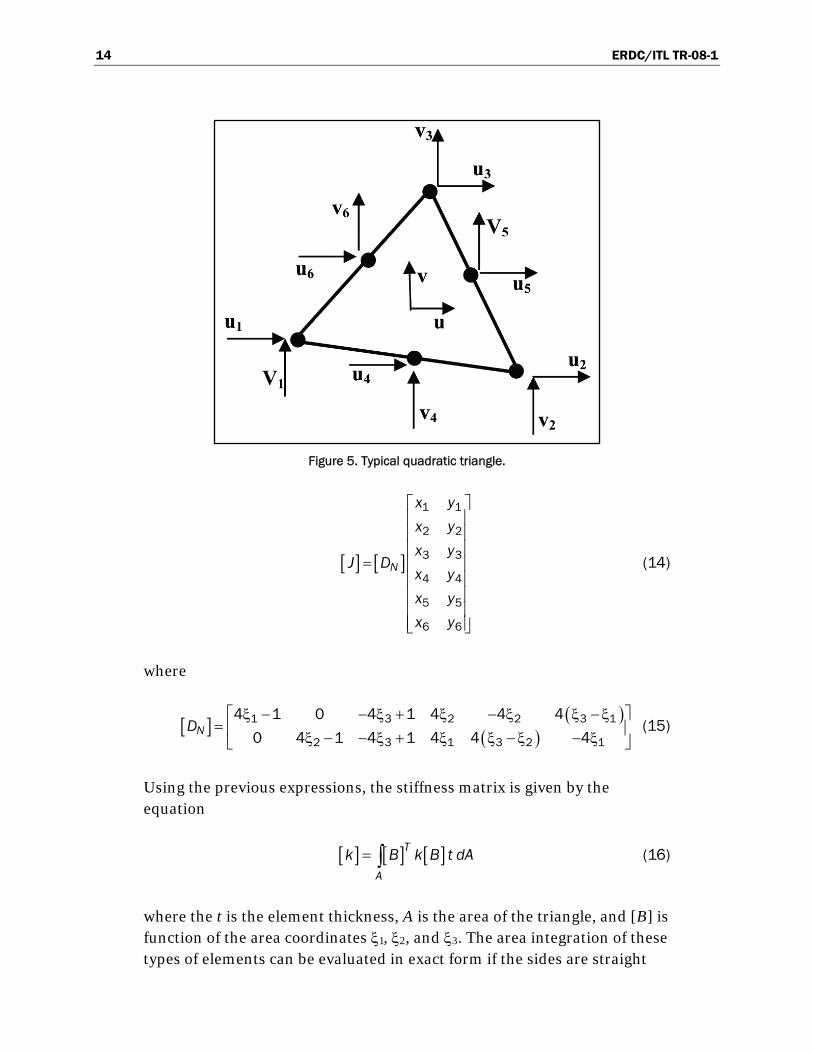
Figure 28. Main window showing the force boundary condition.

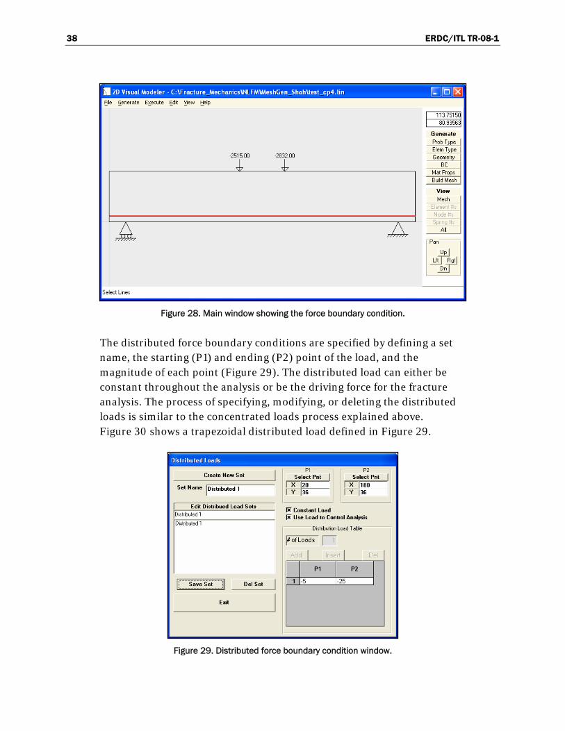
The distributed force boundary conditions are specified by defining a set name, the starting (P1) and ending (P2) point of the load, and the magnitude of each point (Figure 29). The distributed load can either be constant throughout the analysis or be the driving force for the fracture analysis. The process of specifying, modifying, or deleting the distributed loads is similar to the concentrated loads process explained above. Figure 30 shows a trapezoidal distributed load defined in Figure 29.

Figure 29. Distributed force boundary condition window.

ERDC/ITL TR-08-1 39

Figure 30. Main window showing the distributed boundary condition.

Material properties

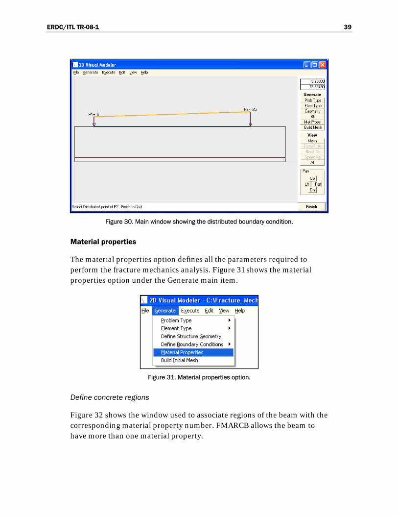
The material properties option defines all the parameters required to perform the fracture mechanics analysis. Figure 31 shows the material properties option under the Generate main item.

Figure 31. Material properties option.

Define concrete regions

Figure 32 shows the window used to associate regions of the beam with the corresponding material property number. FMARCB allows the beam to have more than one material property.

40 ERDC/ITL TR-08-1

Figure 32. Material properties window, define concrete regions option.

Concrete properties

All the required parameters to define the complete concrete softening in compression curve are defined here in addition to the thickness, mass, density, and gravity loading (Figure 33). The elastic modulus of elasticity and the compressive strength ( cf ′ ) are used to determine the elastic strain. Epsilon max represents the strain value where no more compression can be carried by the system.

Gravity loading is equivalent to a body force per unit volume acting within the solid in the direction of the gravity axis. In the formulation used, the gravity axis need not be coincident with either of the coordinate axes, so gravity force components may act in both the x and y directions. The direction in which gravity acts will be defined by specifying the angle that the gravity axis makes with the y axis (Figure 34). The angle is measured counterclockwise between the positive y axis and the tail of the vector that represents the gravity load.

ERDC/ITL TR-08-1 41

Figure 33. Material properties window, concrete properties option.

Figure 34. Description of the angle of the gravity load.

Reinforcement properties

Here, the user specifies the reinforcement material properties, reinforcement area, yield strength, and bar diameter (Figure 35). The user can also define a confinement pressure induced by shear reinforcement.

42 ERDC/ITL TR-08-1

Figure 35. Material properties window, reinforcement properties option.

Bond-slip properties

Figure 36 shows the window used to define the bond-slip parameters.

ERDC/ITL TR-08-1 43

Figure 36. Material properties window, bond-slip properties option.

Fracture properties

Figure 37 shows the window used to describe the parameters required to define the tensile softening curve. The user can choose between a linear or a bilinear curve. Once the tensile strength (ft) and fracture energy (Gf) are defined, the program will calculate and display the tensile softening curve parameters. The user can also input a shear stiffness value. In this example, the shear stiffness value is the same as the initial normal stiffness value. The shear stiffness value is kept constant until the crack opening displacement reaches its critical value, where the interface element is taken off. The fracture properties window also requires the crack size for each crack segment and the distance between nodes along the crack segment. In this example, each crack or crack segment will be 8 in. long, with a total of nine nodes spaced an inch apart.

44 ERDC/ITL TR-08-1

Figure 37. Material properties window, fracture properties option.

Build initial mesh

After all the parameters have been defined, then the initial mesh will be built by choosing the build mesh option on the Generate parameter (Figures 38 and 39). All the above steps required to build the first mesh can also be done using the right-side buttons on the main window (Figure 14). The buttons are organized in the same logical sequence as the Generate option.

Figure 38. Build initial mesh option.

ERDC/ITL TR-08-1 45

Figure 39. Main window showing the quadrilateral mesh.

Execute

At this point, the analysis is ready to be executed (Figure 40). Some final options are required and are shown in Figure 41. The analysis option window allows the user to specify the percentage of error that they are willing to accept for the solution of the non-linear problems. They also need to specify the maximum number of iterations required and which extrapolation method to use.

Figure 40. Main menu, execute command.

46 ERDC/ITL TR-08-1

Figure 41. Analysis options.

Extrapolation of stresses

Two methods to extrapolate the stresses to the nodes are provided in FMARCB. The Average method takes the stresses of the integration points closest to a node and averages them, while the Elegant method uses the shape functions of the element formulation to obtain the stresses. The Elegant method is demonstrated in Figure 42.

ERDC/ITL TR-08-1 47

Figure 42. Extrapolation of stresses to nodes.

Stresses at Gauss points can be interpolated or extrapolated to other points in the element. The result is generally more accurate than the results of evaluating the stresses directly at the point of interest. The extrapolation procedure is as follow:

Treat the Gauss points as if they were nodes of a four-node linear master element with natural coordinates s and r:

= = =ξ

13 or 3

13

r r ξ (39)

= = =η

13 or 3

1

3

r r η (40)

The stresses at any point P in the quadratic master element can be determined using the interpolations function for the linear master element:

σ =∑4

1p N σi i (41)

where σp can be (σxx)p, (σyy)p, or (σxy)p and

48 ERDC/ITL TR-08-1

= ± ±1

(1 )(1 )4iN r s (42)

Thus

σ = − − σ + + − σ + + + σ + − + σ1 2 31 1 1 1

(1 )(1 ) (1 )(1 ) (1 )(1 ) (1 )(1 )4 4 4 4p r s r s r s r s 4 (43)

Run analysis

The analysis can be done without any interruptions by using the Make Complete Analysis option. However, if it is desired, the analysis can be executed manually. The manual option will allow the model to be run one load step at a time. All the steps are specified in a sequence and must be executed before the next load step can be run (Figure 43).

Figure 43. Menu bar, run analysis option.

Edit

This option is used to edit the boundary geometry and the weight of the nodes defined in the Define Structural Geometry option. It can be used to coarsen or refine the mesh in areas of interest or to include additional reinforcement elements (Figure 44).

ERDC/ITL TR-08-1 49

Figure 44. Main menu, edit structural geometry option.

In Figure 45, all the lines and vertices defined in the Define Structural Geometry option are shown. Choosing them and accepting the changes can modify them. Vertices can be added or deleted, and new rebar can also be introduced.

Figure 45. Edit geometry window.

View

The View option (Figure 46) allows the user to see the element numbers, node numbers, and interface elements number. The user can zoom in on any region by using the right-side bottom and return to the whole screen

50 ERDC/ITL TR-08-1

by double clicking the left-side button. The result information can also be obtained by selecting the Element-Node-Spring Data option.

Figure 46. Main menu, view option.

ERDC/ITL TR-08-1 51

6 Example Problem

Introduction

The example presented here is part of a group of numerical analyses conducted by Riveros (2005) and Riveros and Gopalaratnam (2007). They conducted analyses in two sizes of geometrically proportionate reinforced concrete beams (Ghazavy-Khorasgany and Gopalaratnam 1993, Ghazavy-Khorasgany 1994) with normal and high compressive strengths with and without shear reinforcement. The beams were analyzed with shear-span-to-depth ratios (a/d) of 2.5 and 1.5. Figure 47 and Table 1 show the beam size and loading configuration for this example, while Table 2 shows the material properties and parameters used for the numerical computations. The example presented here has normal compressive strength (NSC) without shear reinforcement and a shear-span-to-depth ratio (a/d) of 2.5.

C

d

b

C

Concrete Beam Steel Reinforcement

P L

H

S

L

a PR a

Figure 47. Details of beam geometry and loading configuration.

Table 1. Dimensional details of the reinforced concrete beams.

L, mm (in.) 5486.4 (216.0)

S, mm (in.) 4876.8 (192.0)

H, mm (in.) 914.4 (36.0)

b, mm (in.) 152.4 (6.0)

d, mm (in.) 812.8 (32.0)

a [a/d], mm (in.) 2032.0 [2.5] (80.0)

52 ERDC/ITL TR-08-1

The analysis begins with the definition of the finite element model of the continuum in the elastic state. Once the elastic analysis of the system is completed for the first load step and the principal stresses are extrapolated at the nodes, cracking criteria based on the principal tensile stresses are verified. If the principal tensile stress exceeds the tensile strength, a fictitious crack is incorporated at the location, and automatic remeshing is achieved. Once the system has cracked, the nonlinear solver (Secant Method) is activated. If new cracks and extensions are required after the nonlinear problem satisfies equilibrium for an unbalanced tolerance, the system is remeshed with the new cracks and the existing crack extensions. It is then calibrated again for the same load step until no new cracks or extensions are required. The process is repeated for each load.

Table 2. Material properties experimentally determined by Ghazavy-Khorasgany (1994).

Mix NSC

Age 28 days Test

′cf , MPa (psi) 32.2 (4,668) 43.0 (6,238)

E, MPa (psi) 19,289 (2,797,650) 29,320 (4,252,520)

ft, MPa (psi) 4.3 (618)

Gf , N/mm (lb/in.) 0.10028 (0.57267)

Generation of initial mesh

The following sequence was used to generate the initial mesh:

1. The program is launched, opening the main window (Figure 48).

ERDC/ITL TR-08-1 53

Figure 48. FMARCB main window.

2. For this example without shear reinforcement, a plane stress analysis and four-nodes quadrilateral element have been chosen (Figures 49 and 50).

Figure 49. Program type option.

Figure 50. Element type option.

3. The structure geometry is defined using the line definition window (Figure 51) with the coordinates and weights shown in Table 3. The resulting beam outline is shown in Figure 52.

54 ERDC/ITL TR-08-1

Figure 51. Line definition window.

Figure 52. Main window showing beam boundaries and reinforcement.

ERDC/ITL TR-08-1 55

Table 3. Vertices coordinates and weights for the example.

x, in. y, in. Weight Comments

0.0 0.0 4.0

12.0 0.0 4.0 Left Support

204.0 0.0 4.0 Right Support

216.0 0.0 4.0

216.0 4 4.0 Right side of rebar

216.0 36.0 4.0

124.0 36.0 4.0 Right Load

92.0 36.0 4.0

0.0 36.0 4.0

0.0 4.0 4.0 Left side of rebar

0.0 0.0 4.0

4. Then the displacement boundary conditions are defined. For this example, two displacement boundary conditions exist. The node with coordinate (12,0) is constrained in the y direction, while the node with coordinate (204,0) is constrained in the x and y directions.

The displacement boundary condition of the left-side node has been name BCL, and the one for the right-side node has the name of BCR. Coordinates and direction of the restrained degree of freedom have been defined in the displacement boundary condition window (Figure 53). Figure 54 shows the beam outline with the corresponding displacement boundary conditions.

56 ERDC/ITL TR-08-1

Figure 53. Displacement boundary condition window.

Figure 54. Main window showing the displacement boundary conditions.

5. The force boundary conditions are then defined. For the four-point bending beam, the left loads and right loads are given the names PL and PR, respectively. The magnitudes of the loads were taken from the experiments conducted by Ghazavy-Khorasgany (1994) and are shown in Table 4. For an a/d ration of 2.5 and a distance from the reinforcement to the top fiber (d) of 32 in., the left load is placed at coordinate (92,36) and

ERDC/ITL TR-08-1 57

the right load is placed at (124,36). Figure 55 shows the force boundary condition window with left load, and Figure 56 shows the beam outline with the displacement and load boundary conditions. For this example, the concentrated loads are incremented until failure is reach, so they are used to control the analysis.

Table 4. Load magnitudes for the example.

PL (lb) PR (lb)

−2515 −2832

−3442 −3857

−5005 −5249

−5811 −6055

−6689 −6812

−7153 −7349

Figure 55. Force boundary condition window, left load.

58 ERDC/ITL TR-08-1

Figure 56. Main window showing the force boundary conditions for the example.

6. The material properties for the example are presented in Table 5.

Table 5. Numerical model parameters for the example.

E, GPa (psi) Modulus of elasticity of the concrete 29 (4.25 × 106)

′cf , MPa (psi) Concrete compressive strength 44.8 (6500)

υ Poison ratio 0.18

t, mm (in.) Beam thickness 25.4 (1.0)

ft, MPa (psi) Concrete tensile strength 4.1 (600)

As Area of steel reinforcement 2#8

Es, GPa (psi) Modulus of Elasticity of reinforcement 209 (30 × 106)

fy, MPa (psi) Reinforcement yield strength 462 (67,000)

Gf , N/mm (lb/in.) Fracture energy 0.10028 (0.57267)

wc, mm (in.) Crack opening displacement critical 0.0484 (0.0019)

τmax , MPa (psi) Bond strength 5.5 (800)

u1, mm (in.) Bond slip minimum 0.0127 (0.0005)

u2, mm (in.) Bond slip maximum 1.02 (0.04)

Figure 57 shows the window used to associate regions of the beam with the corresponding material property number. For this example, the entire beam will have the same concrete material properties.

ERDC/ITL TR-08-1 59

Figure 57. Material properties window, concrete regions option.

All the required concrete material properties shown in Table 5 are defined in the concrete properties window (Figure 58) The elastic modulus of elasticity and the compressive strength ( cf ′ ) are used to determine the elastic strain. Epsilon max is set to 0.006, and it represents the strain value where no more compression can be carried by the system.

60 ERDC/ITL TR-08-1

Figure 58. Concrete material properties window for the example.

The reinforcement material properties are shown in Table 5. Note that the reinforcement area for 2 #8 bars is 1.56 in2; however, 0.26 in2 is specified and shown in Figure 59. This is done because the beam width was normalized from 6 in. to 1 in., so the reinforcement was also normalized. The confinement pressure is set to zero because of the absence of shear reinforcement.

ERDC/ITL TR-08-1 61

Figure 59. Material properties window, reinforcement properties option.

Figure 60 shows the definition of the bond-slip parameters. The parameters are also defined in Table 5. In this example the rebar edges are not allow to debond, permitting the hook’s response to be modeled properly. Also, the bond-slip reduction induced by cracking crossing the reinforcement is turned on.

62 ERDC/ITL TR-08-1

Figure 60. Material properties window, bond slip properties option.

Figure 61 shows the fracture parameters definition for this example. The linear softening curve was chosen with the tensile strength (ft) and fracture energy (Gf) values shown in Table 5. The increment of each crack extension is set to 8.0 in., and the extension will have eight, 1-in.-long segments.

ERDC/ITL TR-08-1 63

Figure 61. Material properties window, fracture properties option.

7. Build the Mesh. After all the parameters were defined, the initial mesh (Figure 62) was built by choosing the Build Mesh option on the Generate parameter.

Figure 62. Main window showing the initial (elastic) mesh.

64 ERDC/ITL TR-08-1

Program execution

At this point, the analysis is ready to be executed (Figure 63). Some final options are required and are shown in Figure 64. For this analysis the percentage of unbalance tolerance for the solution of the non-linear problems was set to 5% and the maximum number of iterations to 200.

Figure 63. Main menu, execute command.

Figure 64. Pre-analysis constants and totals window.

Figure 65. Menu bar, make complete analysis option.

ERDC/ITL TR-08-1 65

The analysis was executed without any interruptions by using the Run Complete Analysis option (Figure 65). Figure 66 shows how the first load requires six steps to reach the unbalance equilibrium. Note that the system reaches the unbalance tolerance when all nonlinearities are below the predefined tolerance and when no more new cracks or extensions are formed. Figure 66 also shows how cracks are systematically created, propagated, and meshed. Figures 67 to 70 show the final cracking patterns for the additional load steps. The final cracking pattern is shown in Figure 71.

c

a b

d

e f

g

Figure 66. First load cracking formation sequence.

66 ERDC/ITL TR-08-1

Figure 67. Load 2 cracking pattern.



ERDC/ITL TR-08-1 67


Figure 71. Final cracking pattern.

Analysis and validation of results

The results from the numerical analysis without lateral reinforcement and a shear-span-to-depth ratio of 2.5 indicated a diagonal tension failure after yielding of the longitudinal steel reinforcement. This type of failure was driven by the unstable crack growth of a flexure shear crack. It is suspected that for beams that fail in this manner (post-yielding shear failure), the shear capacity and flexure capacity are nearly equal.

Typically, the load deflection response is linear until the first flexural crack appears in the tension face (Point 1 in Figure 72). Flexural cracks in the inner span of the beam grow in number and size with continued loading. Further loading produces diagonal cracks at the midheight of the beam. This stage in the load-deflection response is denoted as Point 2 in Figure 72. At this load level, the steel begins to debond. With additional load, the bonding capacity deteriorates, reflecting another nonlinear behavior that causes deflections to increase. Also, some flexural cracks that develop in the shear span curve toward midspan at beam midheight. This is shown as Point 3 in Figure 72. Longitudinal steel yielding initiates at Point 4 in Figure 72.

68 ERDC/ITL TR-08-1

05

1015202530354045

0.0 0.2 0.4 0.6 0.8CENTER DEFLECTION (IN.)

LOA

D (K

IPS)

0

50

100

150

2000 5 10 15 20

PLEFTCENTER DEFLECTION (MM)

LOA

D (K

N)

ExperimentFEM Model

12

3

4

a

05

1015202530354045

0.0 0.2 0.4 0.6 0.8CENTER DEFLECTION (IN.)

LOA

D (K

IPS)

0

50

100

150

2000 5 10 15 20

PRIGHTCENTER DEFLECTION (MM)

LOA

D (K

N)

ExperimentFEM Model

1

2

3

4

b

Figure 72. Left and right load displacement curves.

General observations on the crack patterns

Figure 73 shows numerical and experimental cracking patterns of the example. Failure in this beam was observed to be often accompanied by debonding of the longitudinal reinforcement. For an a/d ratio of 2.5, the diagonal cracks were generally z-shaped, often connected with debonding of the longitudinal reinforcement (Figure 73). Debonding starts when the first flexural crack crosses the longitudinal reinforcement and ends with catastrophic diagonal tension shear failure. The general crack and failure patterns obtained from the numerical analysis are comparable with those obtained from the experiments of Ghazavy-Khorasgany (1994).

ERDC/ITL TR-08-1 69

Figure 73. Final cracking pattern results from the numerical model (top) and from the experiments of Ghazavy-Khorasgany (1994).

70 ERDC/ITL TR-08-1

References

Bazant, Z.P. 1985. Comment on Hillerborg’s comparison of size effect law with fictitious crack model. dei Poli Anniversary Volume, Polutecnco di Milano, 335-338.

Bazant, Z.P. 1992. Fracture mechanics of concrete: An apercu of basic concepts and models. First International Conference on Fracture Mechanics of Concrete Structures, Breckenridge, Colorado, 1-5 June 1992, ed. Z.P. Bazant, 145-154, Elsevier Applied Science.

CEB-FIP. 1993. Model Code 1990. Bulletin D’Information 213/214, Comite Euro-International du Beton, Lausanne.

Chang, T.Y., H. Taniguchi, and W.F. Chen. 1987. Nonlinear finite element analysis of reinforcement concrete panels. ASCE, Journal of Structural Engineering 113 (1): 122-138.

Gerstle, W.H., and M. Xie. 1992. FEM modeling of fictitious crack propagation in concrete. Journal of Engineering Mechanics 118 (2): 416-434.

Ghazavy-Khorasgany, M. 1994. Shear failure of normal and high strength RC beams. Ph.D. Dissertation, University of Missouri, Columbia.

Ghazavy-Khorasgany, M., and V.S. Gopalaratnam. 1993. Shear strength of concrete-size and other influences. JCI International Workshop on Size Effect in Concrete Structures, Sendai, Japan, Oct. 31-Nov. 2, 1993.

Gopalaratman, V.S., and B.S. Ye. 1991. Numerical characterization of the nonlinear fracture process in concrete. Engineering Fracture Mechanics 40 (6): 991-1006.

Hayashi, S., and S. Kokusho. 1986. Bond behavior in the neighborhood of the crack. Finite Element Analysis of Reinforced Concrete Structures; Proceedings of the Seminar sponsored by the Japan Society for the Promotion of Science and the U.S. National Science Foundation, Tokyo, Japan, May 21-24, 1985, ed. C. Meyer and H. Okamura, 364-373. New York: American Society of Civil Engineers.

Hillerborg, A. 1983. Fracture mechanics of concrete. Development in Civil Engineering 7. ed. F.H. Wittamann, 223-249. Amsterdam: Elsevier Science Publishers.

Hillerborg, A., M. Modeer, and P.E. Petrson. 1976. Analysis of crack formation and crack growth in concrete by means of fracture mechanics and finite elements. Cement and Concrete Research 6: 773-782.

Hillerborg, A., and J. Rots. 1989. Crack concepts and numerical modeling. In Fracture Mechanics of Concrete Structures, From Theory to Application. ed. L. Elfgren, 128-137. RILEM.

Isenberg, J. 1991. Finite element analysis of reinforced concrete structures II. Proceedings of the International Workshop. NY: American Society of Civil Engineers.

http://www.engineeringvillage2.org/controller/servlet/Controller?CID=quickSearchCitationFormat&searchWord1=%7bGerstle%2C+Walter+H.%7d&section1=AU&database=1&startYear=1969&endYear=2005&yearselect=yearrange&sort=yr

http://www.engineeringvillage2.org/controller/servlet/Controller?CID=quickSearchCitationFormat&searchWord1=%7bXie%2C+Ming%7d&section1=AU&database=1&startYear=1969&endYear=2005&yearselect=yearrange&sort=yr

ERDC/ITL TR-08-1 71

Keuser, M., and G. Mehlhorn. 1987. Finite element models for bond problems. ASCE, Journal of Structuring Engineering 113 (10): 2160-2172.

Mufti, A.A., M.S. Mirza, J.O. McCutcheon, and J. Houde. 1970. A study of the behavior of structural concrete elements. Proceedings of the Special Conference of Finite Element Methods in Civil Engineering. Montreal, Canada.

Ngo, D., and C. Scordelis. 1967. Finite element analysis of reinforcement concrete beams. ACI Journal 64 (14): 152-163.

Nilson, A.H. 1968. Nonlinear analysis of reinforcement concrete by the finite element method. ACI Journal 65 (55): 757-766.

Owen, S.J., M.L. Staten, S.A. Canann, and S. Saigal. 1999. Q-Morph: An indirect approach to advancing front quad meshing. International Journal for Numerical Methods in Engineering 9 (44): 1317-1340.

Petterson, P.E. 1981. Crack growth and development of fracture zone in plane concrete and similar materials. Report No. TVBM-1006. Lund, Sweden: Division of Building Materials, Lund Institute of Technology.

Rashid, Y.R. 1968. Analysis of pre-stressed concrete pressure vessels. Nuclear Engineering Design 7 (4): 334-355.

Riveros, G.A. 2005. Post-cracking behavior of reinforced concrete deep beams: A numerical fracture investigation of concrete strength and beam size. Ph.D. Dissertation, University of Missouri-Columbia.

Riveros, G.A., and V.S. Gopalaratnam. 2007. Fracture behavior of reinforced concrete deep beams: Numerical investigation of strength and beam size. ASCE Structural Journal. In review.

Ruppert, J. 1995. A Delaunay refinement algorithm for quality 2-dimensional mesh generation. Journal of Algorithms 18 (3): 548-585.

Shah, S.P., A. Fafitis, and R. Arnold. 1983. Cyclic loading of spirally reinforced concrete. Journal, Structural Division, ASCE 109 (ST7): 1695-1710.

Van Den Berg, F.J. 1962a. Shear strength of reinforced concrete beams without web reinforcement, Part 1, Distribution of stresses over beam cross section. ACI Journal 59 (11): 1467-1477.

Van Den Berg, F.J. 1962b. Shear strength of reinforced concrete beams without web reinforcement, Part 2, Factors affecting load at diagonal cracking. ACI Journal 59 (11): 1587-1600.

Van Den Berg, F.J. 1962c. Shear strength of reinforced concrete beams without web reinforcement, Part 3, Proposed method for calculating of cracking load. ACI Journal 59 (11): 1849-1861.

Vecchio, F.J., and M.P. Collins. 1986. The modified compression-Field theory for reinforced concrete elements subjected to shear. ACI Journal 83 (2): 219-231.

72 ERDC/ITL TR-08-1

Zhang, M., and O.E. Gjory. 1991. Effect of silica fume on cement hydration in low porosity cement pastes. Cement and Concrete Research 21 (5): 800-808.

Zsutty, T.C. 1968. Beam shear strength prediction by analysis of existing data. ACI Journal 65 (11): 943-951.

Zwoyer, E.M., and C. Siess. 1954. Ultimate strength in shear of simply supported beams without web reinforcement. Journal of the American Concrete Institute 51 (8): 181-200.

ERDC/ITL TR-08-1 73

Appendix A: Output Files

When the analysis is run, a series of directories and files is created. The group of files contain the center displacement for all the loads (*.dsp), the crack and rebar interface element stresses (*.dss), the concrete-steel interface element information (*.RCI), and the GUI input files(*.lin). The program also generates directories that contain files for each of the executions during the non-linear solution calibration. The directories are finite element program input files (INP), finite element program output files (OUT), crack information (CRK), crack interface element (CSE), rebar interface element (RSE), crack report file (RPT), and crack and rebar interface element information (DSS).

DSP file

The DSP file contains loads and displacements for the node at the calculated bottom center of the structure. This DSP file is located in the local directory.

The following is an example of a DSP file: T1_AHW11ONED.DSP.

Loads & Displacement Near Beam Center ( 108.000, 0.000 ) Load #P1DSTRBTD-LD # P2DSTRBTD-LD # @ Node# DeltaC _____________________________________________________________ 1 -5212.00 -7654.00 636 36.55210 2 -6189.00 -8826.00 636 45.39272 3 -9314.00 -12732.00 636 67.53589 4 -12048.00 -16200.00 636 87.07816 5 -15173.00 -20410.00 636 110.23982 6 -18787.00 -23000.00 636 129.40912 6 -18787.00 -23000.00 636 129.40912

DSS file(s)

During each analysis, the DSS file(s) will contain the crack and rebar spring stress and other pertinent information necessary to track the calibration progress. The top section is crack specific, and the bottom section is rebar specific.

A copy of the current DSS file is located in the local directory. The DSS folder, which is a subdirectory of the local directory, contains all the DSS files created during the entire analysis.

74 ERDC/ITL TR-08-1

The following is an abbreviated section of a DSS file: T1_AHW11ONED.DSS.

C:\projects\MSHGEN_QMORPH\MeshGen_LNG\Data\DLOADTST\T1_AHW11\DSS\T1_AHW11ONEDX11_001.dss @ 1/23/2004 2:08:41 PM New Crack Springs - Crack Sprg X Y W1 WCalc SigmaNew SigmaX Knew Kold Wnew Wold Imp % ______________________________________________________________________________________________________________________________ 1 104.000 0.000 0.005785 0.002893 0.00000 30058.000 0.00 0.00 0.005785 0.005785 0.00 2 104.001 0.800 0.005193 0.005193 0.00000 53963.000 0.00 0.00 0.005193 0.005193 0.00 C:\projects\MSHGEN_QMORPH\MeshGen_LNG\Data\DLOADTST\T1_AHW11\DSS\T1_AHW11ONEDX11_001.dss @ 1/23/2004 2:08:41 PM Rebar Springs - Rebar Sprg X Y U1 TauNew Tau1 SigmaX Knew Kold Unew Uold Imp % ______________________________________________________________________________________________________________________________ 6 20.000 4.000 0.06492 264.91132 264.91132 2508.700 1333.33 1333.33 0.064918 0.064918 0.00 7 24.000 4.000 0.06853 295.42142 295.42142 4389.400 1333.33 1333.33 0.068526 0.068526 0.00

CRK file

During each analysis, the CRK file(s) will contain the crack information that is pertinent to the position of the current cracks in the structure. The first line of the file will contain the total number of crack systems. Each crack system consists of the original crack and all of its propagated segments.

There will be a section for each crack system. Each section will start with a line that contains two numbers: the crack system number and the number of crack extensions including the original crack. The next set of lines in the section will contain four values each: the left solid element number, the right solid element number, the left bottom node crack spring number of the left solid element, and the right bottom node crack spring number of the right solid element.

These files are contained in a CRK directory, which is a subdirectory of the local directory.

The following is an example of a CRK file: T1_BNW21X04.CRK.

ERDC/ITL TR-08-1 75

6 1 9 29 56 439 459 105 132 417 442 180 177 402 420 247 250 391 438 293 303 378 414 338 341 360 396 367 362 340 381 392 389 315 362 392 389 341 341

CSE file(s)

During each analysis, the CSE file(s) will contain the crack spring element data. Each file contains pertinent information necessary to track the calibration process of a crack spring element throughout the analysis. The element number is the number denoted at the end of the file name.

These files are located in the CSE directory, which is a subdirectory of the local directory. The CSE directory contains all the CSE files created during the entire analysis.

The following is an abbreviated section of a CSE file: T5_BNW21X02_L00003.CSE.

G:\projects\MSHGEN_QMORPH\MeshGen_LNG\Data\T5_BNW21\CSE\T5_BNW21X02_L00003.CSE New Crack Springs - Crack Sprg X Y W1 WCalc Sig1 SigmaX Knew Kold Wnew Wold Imp % _______________________________________________________________________________________________________________________________ 1 3 28.373 0.000 0.002022 0.001011 0.00000 62.678 0.00 0.00 0.002022 0.002022 0.00 2 3 28.373 0.000 0.002022 0.001011 0.00000 62.678 0.00 0.00 0.002022 0.002022 0.00

RSE file(s)

During each analysis, the RSE file(s) will contain the rebar spring element data. Each file contains pertinent information necessary to track the calibration process of a (rebar spring element throughout the analysis. The element number is the number denoted at the end of the filename.

76 ERDC/ITL TR-08-1

These files are located in the RSE directory or folder, which is a subdirectory of the local directory. The RSE directory contains all the RSE files created during the entire analysis.

The following is an abbreviated section of an RSE file: T5_BNW21X02_L00037.RSE.

G:\projects\MSHGEN_QMORPH\MeshGen_LNG\Data\T5_BNW21\RSE\T5_BNW21X02_L00037.RSE Rebar Springs - Rebar Sprg X Y U1 TauNew Tau1 SigmaX Knew Kold Unew Uold Imp % _______________________________________________________________________________________________________________________________ 13 37 26.880 1.500 0.00015 238.84435 238.84435 241.700 1581096.22 1600000.00 0.000151 0.000000 100.00 14 37 26.880 1.500 0.00017 238.47173 238.47173 267.970 1407048.36 1581096.22 0.000169 0.000151 10.87

RPT file(s)

The RPT file is a crack report file. It contains stress information on nodes due to influence of outside factors such as loads and rebar(s). At the end of each calibration of the current cracks, this file will be generated and used to determine where new cracks will be forming. It also provides information on whether existing cracks will be extended and in what direction.

Each line in the file consist of the following values: Node#, Integration Pnt, xcoord, ycoord, Sigma P1, Sigma P2, ThetaP1, ThetaP2, ThetaC.

These files are located in the RPT directory or folder, which is a subdirectory or folder of the local directory; the RPT directory contains all the RPT files created during the entire analysis.

The following is an example of an RPT File: T5_BNW21X01.RPT.

245 0 15.6800 0.0000 604.4303 4.8295 -1.8208 88.1792 88.1792 250 0 17.9190 0.7490 622.8166 -4.0695 -3.1655 86.8345 86.8345

REPORT DOCUMENTATION PAGE Form Approved

OMB No. 0704-0188 Public reporting burden for this collection of information is estimated to average 1 hour per response, including the time for reviewing instructions, searching existing data sources, gathering and maintaining the data needed, and completing and reviewing this collection of information. Send comments regarding this burden estimate or any other aspect of this collection of information, including suggestions for reducing this burden to Department of Defense, Washington Headquarters Services, Directorate for Information Operations and Reports (0704-0188), 1215 Jefferson Davis Highway, Suite 1204, Arlington, VA 22202-4302. Respondents should be aware that notwithstanding any other provision of law, no person shall be subject to any penalty for failing to comply with a collection of information if it does not display a currently valid OMB control number. PLEASE DO NOT RETURN YOUR FORM TO THE ABOVE ADDRESS.

1. REPORT DATE (DD-MM-YYYY) January 2008

2. REPORT TYPE Final report

3. DATES COVERED (From - To)

5a. CONTRACT NUMBER

5b. GRANT NUMBER

4. TITLE AND SUBTITLE


5c. PROGRAM ELEMENT NUMBER

5d. PROJECT NUMBER

5e. TASK NUMBER

6. AUTHOR(S)

Guillermo A. Riveros, Vellore S. Gopalaratnam, and Amos Chase

5f. WORK UNIT NUMBER

7. PERFORMING ORGANIZATION NAME(S) AND ADDRESS(ES) 8. PERFORMING ORGANIZATION REPORT NUMBER

Information Technology Laboratory, U.S. Army Engineer Research and Development Center, 3909 Halls Ferry Road, Vicksburg, MS 39180-6199; Department of Civil and Environmental Engineering, University of Missouri-Columbia, Columbia, MO 65211; Science Applications International Corporation, 3535 Manor Drive, Suite 4, Vicksburg, MS 39180

ERDC/ITL TR-08-1

9. SPONSORING / MONITORING AGENCY NAME(S) AND ADDRESS(ES) 10. SPONSOR/MONITOR’S ACRONYM(S)

11. SPONSOR/MONITOR’S REPORT NUMBER(S)

12. DISTRIBUTION / AVAILABILITY STATEMENT Approved for public release; distribution is unlimited.

13. SUPPLEMENTARY NOTES

14. ABSTRACT

A finite element package has been developed to perform nonlinear fracture mechanics analysis on reinforced concrete beams. The system consists of a graphic input/output interface and analysis routines using finite element techniques. Fracture Mechanics Analysis of Reinforced Concrete Beams (FMARCB) is a two-dimensional finite element program with triangular, isoparametric, bar, and interface elements. The system uses the discrete crack approach with a fictitious crack model to represent tensile concrete softening; a confinement concrete model to characterize compression softening; a nonlinear bond-slip constitutive model for the bond-slip phenomenon, which is degraded when cracks form across the tensile reinforcement; and an elastic, perfectly plastic constitutive model to represent the yielding of the tensile reinforcement.

15. SUBJECT TERMS Finite element Fracture mechanics

FMARCB Reinforced concrete beams

16. SECURITY CLASSIFICATION OF: 17. LIMITATION OF ABSTRACT

18. NUMBER OF PAGES

19a. NAME OF RESPONSIBLE PERSON

a. REPORT

Unclassified

b. ABSTRACT

Unclassified

c. THIS PAGE

Unclassified 88 19b. TELEPHONE NUMBER (include area code)

Standard Form 298 (Rev. 8-98) Prescribed by ANSI Std. 239.18

Documents

ERDC/ITL TR-08-1, User's Guide: Fracture Mechanics ... · nonlinear fracture mechanics analysis on reinforced concrete beams. The system consists of a graphic input/output interface