Epistemology of Wave Function Collapsein Quantum Physics

Charles Wesley Cowan∗† and Roderich Tumulka∗‡

February 19, 2014

Abstract

Among several possibilities for what reality could be like in view of the empir-ical facts of quantum mechanics, one is provided by theories of spontaneous wavefunction collapse, the best known of which is the Ghirardi–Rimini–Weber (GRW)theory. We show mathematically that in GRW theory (and similar theories) thereare limitations to knowledge, that is, inhabitants of a GRW universe cannot findout all the facts true about their universe. As a specific example, they cannot ac-curately measure the number of collapses that a given physical system undergoesduring a given time interval; in fact, they cannot reliably measure whether oneor zero collapses occur. Put differently, in a GRW universe certain meaningful,factual questions are empirically undecidable. We discuss several types of limita-tions to knowledge and compare them with those in other (no-collapse) versions ofquantum mechanics, such as Bohmian mechanics. Most of our results also applyto observer-induced collapses as in orthodox quantum mechanics (as opposed tothe spontaneous collapses of GRW theory).

Key words: collapse of the wave function; limitations to knowledge; absoluteuncertainty; problems with positivism; empirically undecidable; distinguish twodensity matrices; quantum measurements; foundations of quantum mechanics;Ghirardi–Rimini–Weber (GRW) theory; random wave function.

∗Department of Mathematics, Rutgers University, Hill Center, 110 Frelinghuysen Road, Piscataway,NJ 08854-8019, USA.†E-mail: cwcowan@math.rutgers.edu‡E-mail: tumulka@math.rutgers.edu

1

arX

iv:1

307.

0827

v2 [

quan

t-ph

] 1

9 Fe

b 20

14

Contents

1 Introduction 21.1 Known Examples of Limitations to Knowledge . . . . . . . . . . . . . . . 51.2 Remarks . . . . . . . . . . . . . . . . . . . . . . . . . . . . . . . . . . . . 7

2 Brief Review of GRW Theories 82.1 The GRW Process . . . . . . . . . . . . . . . . . . . . . . . . . . . . . . 82.2 GRWm . . . . . . . . . . . . . . . . . . . . . . . . . . . . . . . . . . . . . 102.3 GRWf . . . . . . . . . . . . . . . . . . . . . . . . . . . . . . . . . . . . . 10

3 First Examples of Limitations to Knowledge in GRW Theories 11

4 Measurements of Flashes in GRWf, or of Collapses in GRWm 124.1 An Example in which ψ is Known . . . . . . . . . . . . . . . . . . . . . . 134.2 Other Choices of ψ . . . . . . . . . . . . . . . . . . . . . . . . . . . . . . 164.3 Experiments Beginning Before t2 . . . . . . . . . . . . . . . . . . . . . . 174.4 If ψ is Random . . . . . . . . . . . . . . . . . . . . . . . . . . . . . . . . 184.5 Optimal Way of Distinguishing Two Density Matrices . . . . . . . . . . . 194.6 If ψ is Unknown . . . . . . . . . . . . . . . . . . . . . . . . . . . . . . . . 20

5 Measurements of m(x) in GRWm 21

A Proofs 23

Science may set limits to knowledge, but should not set limits to imagination.(Bertrand Russell, 1872–1970)

1 Introduction

Since science provides us with knowledge, it may seem surprising that it sometimessets limitations to knowledge. By a “limitation to knowledge” we mean that certainfacts about the world cannot be discovered or confirmed in an empirical way, no matterhow big our effort, including possible future technological advances. For example, alimitation to knowledge is in place if a quantity cannot be measured although it has awell-defined value. A limitation to knowledge means that there is a fact, and we cannotknow what it is, nor even guess with much of a chance of guessing correctly. Natureknows and we do not.

In this paper, we discuss certain limitations to knowledge concerning the collapseof the wave function in quantum physics. Specifically, we investigate limitations tomeasuring whether or not a collapse has occurred. Our results are epistemology in thesense that they concern the possibility of a particular type of knowledge. Since theycan be proved via mathematical theorems, they can be said to fall into the field ofmathematical epistemology. Some preliminary results have been reported in [30].

2

The very idea of a limitation to knowledge may seem to go against the principles ofscience. If there is no way of measuring a quantity X, then this may suggest that X doesnot actually have a well-defined value, i.e., that nature does not know either what X is.For example, in the early days of relativity theory, Lorentz and Fitzgerald proposed thatthe ether causes a length contraction of moving objects, which implies that the speedof earth relative to the ether cannot be measured; however, this situation suggests, asargued by Einstein, that the “speed relative to the ether” is not well defined.

However, the existence of limitations to knowledge is a fact, as it is a simple conse-quence of quantum mechanics, independently of which interpretation of quantum me-chanics we prefer. For example, suppose Alice prepares an ensemble of quantum systems,each with a pure state chosen randomly with distribution µ1 over the unit sphere

S(H ) ={ψ ∈H : ‖ψ‖ = 1

}(1)

in Hilbert space H . Suppose further that µ2 6= µ1 is another distribution over S(H )with the same density matrix, ρµ1 = ρµ2 , where

ρµ =

∫S(H )

µ(dψ) |ψ〉〈ψ| . (2)

Then Bob is unable to determine (even probabilistically) by means of experiments onthe systems whether Alice used µ1 or µ2 (see Appendix A for the proof), while thereis a fact about whether the states actually have distribution µ1 or µ2, as Alice knowsthe pure state of each system. Thus, the predictions of quantum mechanics imply thatthere are facts in the world which cannot be discovered empirically.1

What is upsetting about limitations to knowledge is that they conflict with key ideasof (what may be called) positivism: That a statement is unscientific or even meaninglessif it cannot be tested experimentally, that an object is not real if it cannot be observed,and that a variable is not well-defined if it cannot be measured. We conclude that thisform of positivism is exaggerated; it is inadequate. The above example with Alice andBob refutes it. As an even simpler example against this form of positivism, supposea space ship falls into a black hole; it seems reasonable to believe that it continuesto exist for a while although we cannot observe it any more. While perhaps nobodywould defend positivism as we described it, it is frequently applied in physics reason-ing, particularly in quantum physics—ironically so, since its inadequacy is particularly

1This argument has a curious feature that is worth commenting on. While its goal is to show thatthere is some information that nature knows but no observer can obtain, it actually describes a situationin which Alice (who is an observer, one would guess) is in possession of the relevant information, andonly Bob cannot obtain it—except perhaps by spying out Alice’s notebook! So it may seem that theargument cannot reach its goal. However, the argument does show that there is no way to obtaina certain information about a system from interaction with the system, and that is enough for ourpurposes. Alice then plays the role of proving (to a positivist) that that information objectively exists.Alternatively, one could also argue as follows. If Alice destroyed the records of the states she preparedthen nobody would know, while it seems plausible that nature still knows the states (since it seemsimplausible that the states would suddenly become indefinite if Alice burns her notebook). Thus, theexample also easily provides a case in which nobody is in possession of the relevant information.

3

clear in quantum physics, as the example with Alice and Bob shows. Needless to say,positivism is also unnecessary in quantum physics, as demonstrated by the viability of“realist” interpretations of quantum mechanics (“quantum theories without observers”)such as Bohmian mechanics [11, 28], spontaneous collapse theories [24, 8, 36, 16, 22],and perhaps (some versions of) many-worlds [21, 40, 4].

It is sometimes suggested that a theory is unconvincing if it entails limitations toknowledge. We do not share this sentiment. On the contrary, we think it is hard todefend in view of the considerations around (2).

In this paper, we deal primarily with spontaneous collapse theories, concretely withthe simplest and best-known one, the Ghirardi–Rimini–Weber (GRW) theory [24, 8] inthe versions GRWm [16, 10, 27] and GRWf [8, 38]; for an introduction see, e.g., [3, 8, 22].We briefly review GRW theory in Section 2. Quantum theories without observers haveno need for the orthodox quantum philosophy of “complementarity.” In these theories,it is clear what is real. And thus, the possibility arises that certain things that are realcannot be observed.

It is necessary to distinguish between quantum measurements and (what we call)genuine measurements. Quantum measurements are not literally measurements in theordinary sense, i.e., they are not experiments for discovering the values of variables thathave well-defined values.2 In contrast, in a quantum theory without observers there areseveral variables that are supposed to have well-defined values, and we may ask whetherand how we could measure these: for example, the wave function ψ, the matter densitym(x, t) in GRWm, the flashes in GRWf. We call experiments discovering these valuesgenuine measurements.

We show that certain well-defined variables in GRW theories do not permit genuinemeasurements; that is, that certain facts in GRW worlds cannot be found out by theinhabitants of those worlds. At the same time, there is no way of replacing the GRWtheories with simpler and more parsimonious theories by merely denying the factualcharacter of what the inhabitants cannot find out,3 much in contrast to an unobservableether whose existence can very well be denied.

These limitations to knowledge arise as a consequence of the defining equations ofthe theories. They are not further, ad hoc postulates; and they do not require carefullycontrived, or conspiratorial, initial conditions. Instead, they are dictated by the physicallaws. The GRW theories thus exemplify Einstein’s dictum that “it is the theory whichdecides what can be observed” [20]. The situation is in a way parallel to that of blackholes, where also the physical law itself (in that case, the Einstein equation of general

2Indeed, it is the content of the “no-hidden-variable theorems” such as Gleason’s and Kochen–Specker’s that one cannot think of the outcomes of quantum measurements as values that were alreadyknown to nature before the experiment, and merely made known to us by the experiment.

3That is, if, in reaction to our result that the flashes cannot be measured accurately, one droppedthe flashes from the reality, then one would end up with the GRW wave function without a primitiveontology, which is not a satisfactory physical theory [33, 34, 3, 32, 1, 2]. Likewise, if, in reaction to ourresult that the number of collapses in a given time interval [t1, t2] cannot be accurately measured, onedecided that there is no fact about the number of collapses in [t1, t2], then one would have to drop theGRW law of wave function evolution, and thus leave the framework of GRW theories.

4

relativity) implies that observers outside the black hole cannot find out what happensinside. We emphasize that the limitations of knowledge in GRW theories do not in anyway represent a drawback of these theories.

This paper is organized as follows. In the remainder of Section 1, we provide back-ground on the concept of a limitation to knowledge by describing examples. In Section 2we review the definition of the GRW theories. In Section 3 we introduce our main tooland prove, as a first result, that the function m(x) in GRWm cannot be measured withmicroscopic accuracy. In Section 4 we present detailed results about the accuracy withwhich a collapse can be detected. In Section 5 we investigate the accuracy with whichthe function m(x) in GRWm can be measured.

1.1 Known Examples of Limitations to Knowledge

1. Some limitations to knowledge are quite familiar: It is impossible to look into thefuture (e.g., to find out next week’s stock prices in less time than a week), to lookdirectly into the past (e.g., to determine systematically who Jack the Ripper was),to look into a spacelike separated region (superluminal signaling), or to look intoa black hole.

2. Quantum theory is particularly rich in limitations to knowledge, as exemplifiedby items 2–10 in this list. To begin with, as already mentioned, it is impossibleto distinguish empirically between two different ensembles of wave functions withthe same density matrix.

3. It is impossible to measure the wave function of an individual system. For exam-ple, if Alice chooses a direction in space and prepares a single particle in a purespin state pointing in this direction then Bob cannot determine this direction bymeans of whichever experiment on the particle. The best Bob can do is a Stern–Gerlach experiment in (say) the z direction, which yields one bit of informationand tells Bob whether Alice’s chosen direction is more likely to lie in the upper orlower hemisphere. Bob can do better if Alice prepares N � 1 disentangled par-ticles, each in the same pure spin state; by means of Stern–Gerlach experimentsin different directions and a statistical analysis of the results, he can estimate thedirection with arbitrary accuracy (with high probability) for sufficiently large N .(It is sometimes suggested that “protective measurements” can measure the wavefunction. However, these experiments involve a mechanism that restores the initialwave function ψ0 of the system after a (weak) interaction with the apparatus, andmany repetitions of the procedure. Thus, in effect, the apparatus is provided withmany copies of the same wave function ψ0, so that the possibility of determiningψ0 is in agreement with what we said earlier in this paragraph.)

4. A different type of limitation to knowledge comes up in quantum cryptography,specifically in quantum key distribution: The eavesdropper Eve cannot obtainuseful information about the key created by Alice and Bob using a quantum keydistribution scheme without leaving traces that Alice and Bob can detect.

5

5. “Absolute uncertainty” in Bohmian mechanics [17]: Given that the (conditional)wave function of a system is ψ, it is impossible for an inhabitant of a Bohmianuniverse to know the system’s configuration more accurately than allowed by the|ψ|2 distribution. If the configuration gets measured more accurately, then theconditional wave function becomes narrower. (However, while Bohmian mechanicsputs limitations to knowing the configuration, it still allows in principle to measurethe configuration with arbitrary accuracy; thus, the access to the configuration isless restricted than the one to the m function in GRWm, which, as we show inSection 3, cannot be measured with microscopic accuracy.)

6. It is impossible to measure the velocity of a particle in Bohmian mechanics [18, 19](except when information about the wave function is given). That is, there is nomachine into which we could insert a particle with arbitrary wave function ψ andwhich would display correctly the velocity of the particle (i.e., the velocity rightbefore the experiment). Note that the measurement of velocity would amount to(what we called) a genuine measurement, not a quantum measurement.

It is possible, in contrast, to build a machine that will correctly measure the ve-locity if the machine is told what ψ is; for example, the machine could measurethe position of the particle (to sufficient accuracy) and then compute the velocityusing Bohm’s equation of motion. It is also in principle possible to build a ma-chine that correctly displays the velocity after the experiment without being giveninformation about the wave function ψ before the experiment; a formal quantummeasurement of the momentum observable achieves this. It is also possible tobuild a machine that correctly displays the velocity for a limited set of ψs (suchas approximate momentum eigenstates, i.e., wide packets of plane waves).

7. It is impossible to distinguish empirically between certain different versions ofBohmian mechanics [29, 15], all of which lead to the appropriate |ψ|2 distribu-tion for macroscopic configurations, or between Bohmian mechanics and Nelson’sstochastic mechanics [35, 26], or (presumably) between Bohmian mechanics andsome versions of the many-worlds theory [4].

8. It is impossible to distinguish empirically between GRWm and GRWf [3, 30].

9. The study of Colin et al. on superselection rules [12] identified cases in GRWmin which a “weak” but no “strong” superselection rule holds, which means thatfor every superposition ψ (of eigenvectors of the superselected operator) there isa mixture µ (of eigenvectors) that cannot be empirically distinguished from ψ,while µ leads to different histories of the primitive ontology (PO, or local beables)than ψ. As a consequence, the difference between the PO arising from ψ and thatarising from µ cannot be detected empirically. The concrete example in GRWmamounts more or less to the fact that the m function cannot be measured withmicroscopic accuracy.

6

10. Whether the Heisenberg uncertainty relation is or is not an instance of a limitationto knowledge, depends on the precise version of quantum mechanics used.

In Bohmian mechanics, it is: Certain standard experiments realizing a “quantummeasurement of the momentum observable” (such as letting a particle move freelyfor a long time t, then measuring its position Q(t) to sufficient accuracy, andmultiplying by m/t) actually measure (mass times) the long-time average of theBohmian velocity, u = limt→∞Q(t)/t, which is a deterministic function of theinitial position Q(0) and the initial wave function ψ0, u = u(Q(0), ψ0). TheHeisenberg uncertainty relation implies that for a Bohmian particle with positionQ and wave function ψ, even if ψ is known, the values of Q and u(Q,ψ) cannotboth be known with arbitrary accuracy, although both quantities have precisevalues in reality.4

In collapse theories such as GRWm and GRWf, in contrast, there is no precise valueof either the position or the momentum observable before E , if E is an experimentthat can be regarded as a “quantum measurement of position or momentum.” Inparticular, E is not a measurement in the literal sense. Rather, the outcome ofsuch an experiment is a random value that is only generated in the course of theexperiment. Since, as long as no such experiment is carried out, there is no factabout the value of the position or the momentum observable, there is nothing tobe ignorant of. As a consequence, the Heisenberg uncertainty relation does notconstitute a limitation to knowledge in GRW theories.

11. Chaos leads to practical limitations: If the behavior of a (classical) dynamicalsystem depends sensitively on the initial conditions, and if our knowledge of theinitial conditions has limited accuracy, then we may be unable to predict the be-havior although the system is deterministic in principle. This fact can be regardedas a limitation to knowledge, too, but there is a fundamental difference to the lim-itations of knowledge discussed in this paper: There is no reason in sight for whythis limitation should be unsurmountable. If we are willing to make a bigger effortwhen measuring the initial conditions so as to obtain higher accuracy, and if weare willing to make a bigger effort in the computation of predictions, then we maybe able to predict the behavior of the system for a longer time interval.

1.2 Remarks

1. There are parallels between the limitations to knowledge discussed in this pa-per and Godel’s incompleteness theorem [25]. While Godel’s theorem concerns amathematical statement that is formally undecidable, our results concern physicalstatements that are empirically undecidable. The distinction between true and

4It is possible, however, to measure Q (to sufficient accuracy) and then calculate u(Q,ψ) if ψ isknown. Since this measurement will change the wave function, it is afterwards still not known whatthe present value of u is; we only obtain information about what u(Q,ψ) was before the measurement,not about what it is now after the measurement.

7

provable in mathematics resembles the distinction between real and observablein physics. Mathematical platonism, which can be described as the view that amathematical statement can be true even if it is not provable, is parallel to realism,which can be described as the view that something can be a physical fact evenif it is not observable; mathematical formalism, the opposite view, is parallel tophysical positivism. A basic difference between Godel’s theorem and our resultsis that we can know the truth value of Godel’s undecidable statement: it is true.That is, while the truth value is unknowable to the formal system, it is knowableto us. Thus, the situation of Godel’s undecidable statement is more analogous tothat of the physical laws (as discussed in item 7 above) than to that of measuring,say, the number of collapses. Namely, while we often have no more informationabout the number of collapses than its a priori probability distribution, we maybe able to guess the physical laws, and thus prefer one among several empiricallyequivalent theories, on the basis of the simplicity, naturalness, elegance, and plau-sibility of the theory, even though our intuition will not provide as reliable andclear a decision as about the truth value of Godel’s undecidable statement. Fi-nally, we note that there may be, besides Godel’s statement, other examples offormally undecidable statements that leave us completely and permanently in thedark as to what their truth values are.

2. There are also parallels between the limitations to knowledge discussed in thispaper and Carnot’s theory of heat engines: Not all of the energy contained in asystem can be extracted in a useful form (i.e., as work); not all of the informationcontained in a system can be extracted in a useful form (i.e., as human knowledge).By the latter statement we mean that not all of the facts true of a system can befound out empirically.

2 Brief Review of GRW Theories

2.1 The GRW Process

In both the GRWm and the GRWf theory the evolution of the wave function follows,instead of the Schrodinger equation, a stochastic jump process in Hilbert space, calledthe GRW process. Consider a quantum system of (what would normally be called) N“particles,” described by a wave function ψ = ψ(q1, . . . , qN), qi ∈ R3, i = 1, . . . , N . TheGRW process behaves as if an “observer” outside the universe made unsharp “quantummeasurements” of the position observable of a randomly selected particle at randomtimes T1, T2, . . . that occur with constant rate Nλ, where λ is a new constant of natureof order of 10−16 s−1, called the collapse rate per particle. The wave function “collapses”at every time T = Tk, i.e., it changes discontinuously and randomly as follows. Thepost-collapse wave function ψT+ = limt↘T ψt is obtained from the pre-collapse wavefunction ψT− = limt↗T ψt by multiplication by a Gaussian function,

ψT+(q1, . . . , qN) =1

Ngσ(qI −X)1/2 ψT−(q1, . . . , qN) , (3)

8

where

gσ(x) =1

(2πσ2)3/2e−

x2

2σ2 (4)

is the 3-dimensional Gaussian function of width σ, I is chosen randomly from 1, . . . , N ,and

N = N (X) =

(∫R3N

dq1 · · · dqN gσ(qI −X) |ψT−(q1, . . . , qN)|2)1/2

(5)

is a normalization factor. The width σ is another new constant of nature of order of10−7 m, while the center X = Xk is chosen randomly with probability density

ρ(x) = N (x)2 . (6)

We will refer to (Xk, Tk) as the space-time location of the collapse.Between the collapses, the wave function evolves according to the Schrodinger equa-

tion corresponding to the standard Hamiltonian H governing the system, e.g., given, forN spinless particles, by

H = −N∑i=1

~2

2mi

∇2qi

+ V, (7)

where mi, i = 1, . . . , N , are the masses of the particles, and V is the potential energyfunction of the system. Due to the stochastic evolution, the wave function ψt at time tis random.

This completes our description of the GRW law for the evolution of the wave function.According to the GRW theories, the wave function ψ of the universe evolves according tothis stochastic law, starting from the initial time (say, the big bang). As a consequence[5, 30], a subsystem of the universe (comprising M < N “particles”) will have a wavefunction ϕ of its own that evolves according to the appropriate M -particle version ofthe GRW process during the time interval [t1, t2], provided that ψ(t1) = ϕ(t1) ⊗ χ(t1)and that the system is isolated from its environment during that interval.

We now turn to the primitive ontology (PO), that is, the part of the ontology (i.e.,of what exists, according to the theory) that represents matter in space and time (andof which macroscopic objects consist), according to the theory. Without such furtherontology, the GRW theory would not be satisfactory as a fundamental physical theory[33, 34, 3, 32, 1, 2]. In the subsections below we present two versions of the GRW theory,based on two different choices of the PO, namely the matter density ontology (GRWmin Section 2.2) and the flash ontology (GRWf in Section 2.3).

9

2.2 GRWm

GRWm postulates that, at every time t, matter is continuously distributed in space withdensity function m(x, t) for every location x ∈ R3, given by

m(x, t) =N∑i=1

mi

∫R3N

dq1 · · · dqN δ3(qi − x)∣∣ψt(q1, . . . , qN)

∣∣2 (8)

=N∑i=1

mi

∫R3(N−1)

dq1 · · · dqi−1 dqi+1 · · · dqN∣∣ψt(q1, . . . , qi−1, x, qi+1, . . . , qN)

∣∣2 . (9)

In words, one starts with the |ψ|2–distribution in configuration space R3N , then obtainsthe marginal distribution of the i-th degree of freedom qi ∈ R3 by integrating out allother variables qj, j 6= i, multiplies by the mass associated with qi, and sums over i.Alternatively, (8) can be rewritten as

m(x, t) = 〈ψt|M(x)|ψt〉 (10)

withM(x) =

∑i

mi δ3(Qi − x) (11)

the mass density operator, defined in terms of the position operators Qiψ(q1, . . . , qN) =qi ψ(q1, . . . , qN).

2.3 GRWf

According to GRWf, the PO is given by “events” in space-time called flashes, mathe-matically described by points in space-time. What this means is that in GRWf matteris neither made of particles following world lines, nor of a continuous distribution ofmatter such as in GRWm, but rather of discrete points in space-time, in fact finitelymany points in every bounded space-time region.

In the GRWf theory, the space-time locations of the flashes can be read off from thehistory of the wave function: every flash corresponds to one of the spontaneous collapsesof the wave function, and its space-time location is just the space-time location of thatcollapse. The flashes form the set

F = {(X1, T1), . . . , (Xk, Tk), . . .} (12)

(with T1 < T2 < . . .). Alternatively, we may postulate that flashes can be of N differenttypes (“colors”), corresponding to the mathematical description

F = {(X1, T1, I1), . . . , (Xk, Tk, Ik), . . .} , (13)

with Ik the number of the particle affected by the k-th collapse.

10

Note that if the number N of degrees of freedom in the wave function is large, as inthe case of a macroscopic object, the number of flashes is also large (if λ = 10−15 s−1 andN = 1023, we obtain 108 flashes per second). Therefore, for a reasonable choice of theparameters of the GRWf theory, a cubic centimeter of solid matter contains more than108 flashes per second. That is to say that large numbers of flashes can form macroscopicshapes, such as tables and chairs. That is how we find an image of our world in GRWf.

We should remark that the word “particle” can be misleading. According to GRWf,there are no particles in the world, just flashes and a wave function. According toGRWm, there are no particles, just continuously distributed matter and a wave function.The word “particle” should thus not be taken literally (just like, e.g., the word “sunrise”);we use it only because it is common terminology in quantum mechanics.

3 First Examples of Limitations to Knowledge in

GRW Theories

An important tool for the analysis of limitations to knowledge is the main theorem aboutPOVMs, which says that for every experiment E on a system “sys” there is a POVM(positive-operator-valued measure5) E on the value space of E acting on the system’sHilbert space Hsys such that if sys has wave function ψ and E is carried out then theoutcome Z has probability distribution

P(Z = z) = 〈ψ|Ez|ψ〉 . (14)

This theorem has been proven for Bohmian mechanics [18], GRWf [39, 30], and GRWm[30]; a similar result for GRWm can be found in [6]. In orthodox quantum mechanics,the theorem is true as well, taking for granted that, after E , a quantum measurementof the position observable of the pointer of E ’s apparatus will yield the result of E .

From the main theorem about POVMs we can deduce a first limitation to knowledge[30]: that it is impossible to measure the matter density m(x, t) in GRWm. Moreprecisely, it is impossible to build a machine that will, when fed with a system with anywave function ψ, determine m(x). This is because the outcome Z of any experiment ina GRW world has a probability distribution P(Z = z) whose dependence on the wavefunction is quadratic, 〈ψ|E(z)|ψ〉, while the m(x) function (or, in fact, any functional ofthe wave function) is deterministic in ψ, that is, its probability distribution is a Diracdelta function and not quadratic.6 This result notwithstanding, it is possible to measure

5A POVM is a family of positive operators Ez such that∑z Ez = I, the identity operator. It

is also known as a generalized observable and in fact generalizes the notion of a quantum observablerepresented by a self-adjoint operator A, which applies to an ideal quantum measurement. For an idealquantum measurement, the values z are the eigenvalues of A and Ez is the projection to the eigenspace.

6The fact that the deterministic value of m(x) is given by a quadratic expression in ψ, viz. (8),should not be confused with the condition that the probability distribution of m(x) depend on ψ in aquadratic way.

11

m(x) with limited accuracy, that is, to measure a macroscopic, coarse-grained versionof m(x); this we will study in Section 5.

The same type of argument shows [30] that it is impossible to measure the wavefunction ψt of a system in either GRWm or GRWf (or in Bohmian mechanics, many-worlds, or orthodox quantum mechanics, for that matter).

Let us compare the situation in GRW theories to that of Bohmian mechanics. Asmentioned above, the velocity of a given Bohmian particle is not measurable. On theother hand, there is no limitation in principle in Bohmian mechanics to measuringthe position of a particle to arbitrary accuracy, except that doing so will alter theparticle’s (conditional) wave function, and thus its future trajectory. Here we encountera basic difference between Bohmian mechanics and GRWm: the configuration of theprimitive ontology can be measured in Bohmian mechanics but not in GRWm. (InBohmian mechanics, the configuration of the primitive ontology corresponds to thepositions of all particles, while in GRWm it corresponds to the m(x, t) function for allx ∈ R3.) In GRWf, for comparison, there is nothing like a configuration of the primitiveontology at time t, of which we could ask whether it can be measured. There is only aspace-time history of the primitive ontology, which we may wish to measure. Bohmianmechanics is an example of a world in which the history of a system cannot be measuredwithout disturbing its course, and indeed disturbing it all the more drastically the moreaccurately we try to measure it. This suggests already that also in GRWf, measuringthe pattern of flashes will entail disturbing it—and thus finding a pattern of flashesthat is different from what would have occurred naturally (i.e., without intervention),so that this experiment could not be regarded as a genuine measurement of the patternof flashes.

4 Measurements of Flashes in GRWf, or of Col-

lapses in GRWm

Even if we accept disturbances, the following heuristic reasoning suggests that individualflashes cannot be detected. Suppose we had an apparatus capable of detecting flashesin a system. Think of the wave function of system and apparatus together as a func-tion on configuration space R3N , and think of configurations as one would in Bohmianmechanics. Let R0 be the set of those configurations q such that in a Bohmian world inconfiguration q the apparatus display reads “no flash detected so far,” and let R1 be theset of those configurations in which the display reads “one flash detected so far.” ThenR1 is disjoint from R0. Recall that a flash in the system leads to a change in the wavefunction of the form

ψ → ψ′ =1

Ngσ(qi − x)1/2 ψ . (15)

But such a change does not push the wave function from R0 to R1. That is, if ψ, as afunction on R3N , is concentrated in the region R0, then ψ′ as given by (15) will not beconcentrated in R1; instead, it is still concentrated in (some subset of) R0.

12

While the macroscopic equivalence class7 of the pattern of flashes is measurable, weare led to suspecting that the microscopic details of the pattern are not. In what senseexactly that is or is not the case will be discussed in this section.

Note first that the main theorem about POVMs does not directly exclude measure-ments of F , the pattern of flashes, in the way it directly excluded measurements of m(x)or ψ. After all, the argument was that the probability distribution of m(x) or ψ does notdepend quadratically on ψ. The probability distribution of F , in contrast, does dependon ψ in a quadratic way: There is a continuous POVM G(f) on the space of all flashhistories f such that the probability density of F is given by

P(F = f) = 〈ψ|G(f)|ψ〉 , (16)

with ψ the initial wave function [39, 30]. Of course, this fact does not imply that F canbe measured—and we are claiming that it cannot.

To approach the question whether one can detect an individual flash (or an individualcollapse in GRWm), we begin with a simple example.

4.1 An Example in which ψ is Known

Suppose ψ is the wave function of a single particle and a superposition of two wavepackets with disjoint supports in space,

ψ = 1√2|here〉+ 1√

2|there〉 , (17)

as may result from a double-slit setup. (The reasoning that is to follow will also applyto a molecule or small solid body with |here〉 and |there〉 differing by a shift in thecenter-of-mass coordinate that makes their supports disjoint.) Suppose, for simplicity,that the Hamiltonian of the system vanishes, so that the Schrodinger time evolutionis trivial. We ask whether any flash at all occurs during the time interval [t1, t2]. Weare interested in the case in which the probability of a flash is neither close to 1 norclose to 0, a case that can be arranged by suitable choice of the duration t2− t1. (For asingle particle, this choice might mean the duration is millions of years; we might eitherconsider this case as a theoretical exercise, or consider instead the center-of-mass of amany-particle system to reduce the duration. To obtain a reasonable duration, we maywant to consider the case that the number of particles is big (say, > 1010) but not toobig (say, < 1020); anyway, that makes no difference to the theoretical analysis.)

For simplicity, we ignore the possibility of multiple collapses and assume that acollapse occurs with probability p, and no collapse with probability 1−p. Let us furtherassume that the two packets |here〉 and |there〉 have width less than σ but separationgreater than σ, so that after collapse the wave function is either approximately |here〉or approximately |there〉. For simplicity, let us assume that after collapse the wave

7Consider two patterns of flashes in space-time. We call them macroscopically equivalent if they lookalike on the macroscopic level. While the notion of macroscopic equivalence is not precisely defined, itis roughly defined.

13

function is either exactly |here〉 or exactly |there〉, each with probability 1/2. Thus thefinal wave function ψ′ is distributed according to

P(ψ′ = ψ) = 1− p ,P(ψ′ = |here〉) = p/2 (18)

P(ψ′ = |there〉) = p/2 .

Let C ∈ {0, 1} be the random number of collapses.We ask whether and how well an experiment beginning at time t2 can decide whether

a collapse has occurred. This amounts essentially to distinguishing between the threevectors |here〉, |there〉, and ψ. While |here〉 and |there〉 are orthogonal, ψ is not or-thogonal to either. As is well known, it is not possible to distinguish reliably betweennon-orthogonal vectors. (Our question can also be regarded as a special case of thequestion how well an experiment can distinguish between two density matrices ρ1, ρ2;see Section 4.5.)

The following experiment E1 provides probabilistic information about C: carry outa “quantum measurement of the observable” E1 given by the projection to the 1-dimensional subspace orthogonal to that spanned by (17),

E1 = I − |ψ〉〈ψ| (19)

with I the identity operator. If the result Z was 1, then it can be concluded thata collapse has occurred, C = 1. (Because if no collapse has occurred, then ψ′ = ψand Z = 0 with probability 1.) If the result Z was 0, nothing can be concluded withcertainty (since also |here〉 and |there〉 lead to a probability of 1/2 for the outcome tobe 0). However, in this case the (Bayesian) conditional probability that a collapse hasoccurred is less than p (and thus Z is informative about C):

P(C = 1|Z = 0) =P(C = 1, Z = 0)

P(C = 1, Z = 0) + P(C = 0, Z = 0)(20)

=P(Z = 0|C = 1)P(C = 1)

P(Z = 0|C = 1)P(C = 1) + P(Z = 0|C = 0)P(C = 0)(21)

=12p

12p+ 1 · (1− p)

=p

2− p< p . (22)

Thus, in every case the experiment can retrodict C with greater precision than it couldhave been predicted a priori (i.e., than attributing probability p to a collapse and 1− pto no collapse).

To quantify the usefulness of the experiment, we define the reliability R(E ) of ayes-no experiment (or 1-0 experiment) E as the probability that it correctly retrodictswhether a collapse has occurred,

R(E ) = P(Z = 0, C = 0) + P(Z = 1, C = 1) (23)

= P(Z = 0|C = 0)P(C = 0) + P(Z = 1|C = 1)P(C = 1) . (24)

14

For the particular experiment E1 just described, we find that P(Z = 0|C = 0) = 1,P(C = 0) = 1− p, P(Z = 1|C = 1) = 1

2, and P(C = 1) = p, so

R(E1) = 1− p

2. (25)

(See Proposition 9 in Appendix A for a more general result.) The fact that this quantityis less than 1 means that this experiment cannot decide with certainty whether a collapsehas occured.

Proposition 1. [13] For the initial wave function (17) and 0 ≤ p ≤ 2/3, no experimentat time t2 can retrodict C with greater reliability than the quantum measurement ofE1 = I − |ψ〉〈ψ|:

∀E ∀p ∈ [0, 23] : R(E ) ≤ 1− p

2. (26)

In particular, for p 6= 0 it is impossible to determine with reliability 1 whether a collapsehas occurred or not.

The proof [13] of this proposition relies, of course, on the main theorem aboutPOVMs, which associates with every yes-no experiment (acting on a system with wavefunctions that are superpositions of |here〉 and |there〉) a positive semi-definite 2 × 2matrix E (namely, E = Eyes, while Eno = I − Eyes). The proof shows that there is nosuch matrix E for which R exceeds 1 − p/2. We note that R(E ) depends on E onlythrough E, that is, two experiments with the same POVM have the same reliability (seeProposition 9 in Appendix A).

Proposition 1 expresses a limitation to knowledge: Although we can empiricallygain some information about the value of C, we cannot obtain full information, i.e.,we cannot measure C with certainty. In fact, not even close to certainty: While themaximal reliability 1 − p/2 is close to 1 if p is small, in this case it is easy to guesscorrectly without any experiment whether a collapse occurred: no. In other words, thereliability 1− p/2 can be put into perspective by comparing it to that of blind guessing,i.e., of the experiment E∅ that does not even interact with the system but always answers“no” if p ≤ 1/2 and always “yes” if p > 1/2. (We think of p as known.) This experiment(which corresponds to E = 0 if p ≤ 1/2 and to E = I if p > 1/2) has reliability

R(E∅) = max{p, 1− p} . (27)

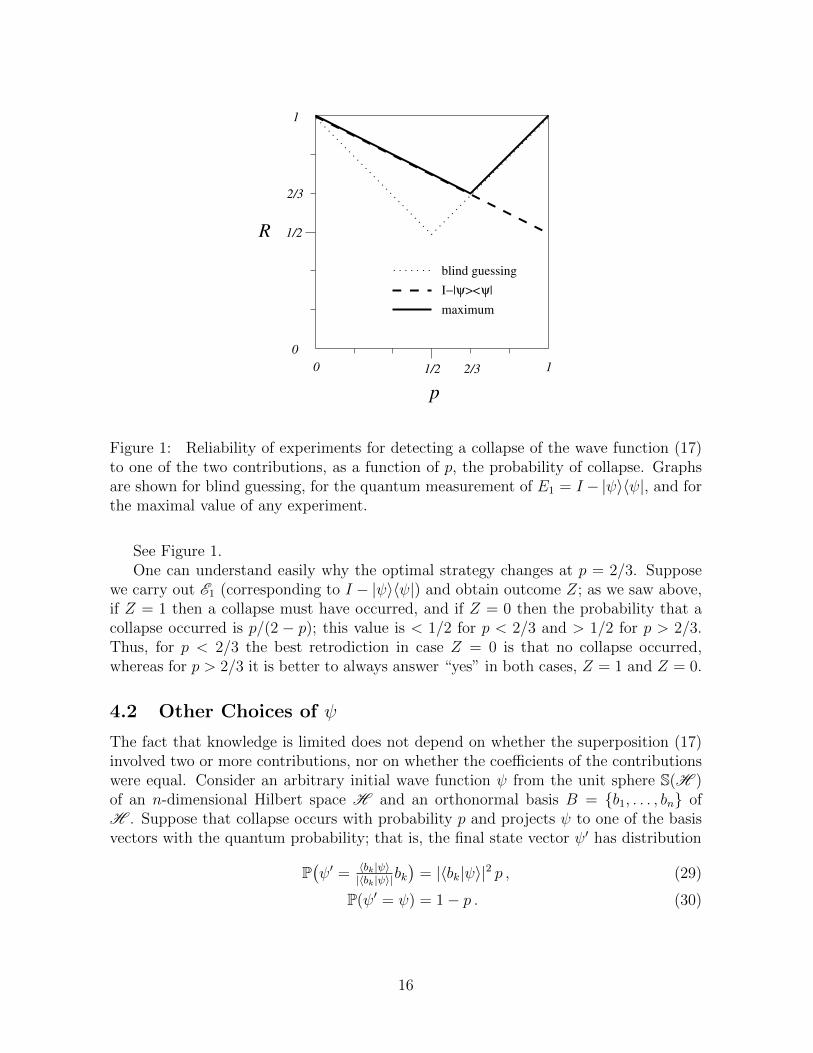
For 0 ≤ p ≤ 1/2, the optimal reliability is right in the middle between the trivialachievement R = 1−p and the desired achievement R = 1; for 1/2 ≤ p ≤ 2/3, it is evencloser to the trivial achievement R = p. For p > 2/3, the situation is even worse:

Proposition 2. [13] For ψ as in (17) and 2/3 ≤ p ≤ 1, no experiment at time t2 canretrodict C with greater reliability than blind guessing:

∀E ∀p ∈ [23, 1] : R(E ) ≤ p . (28)

15

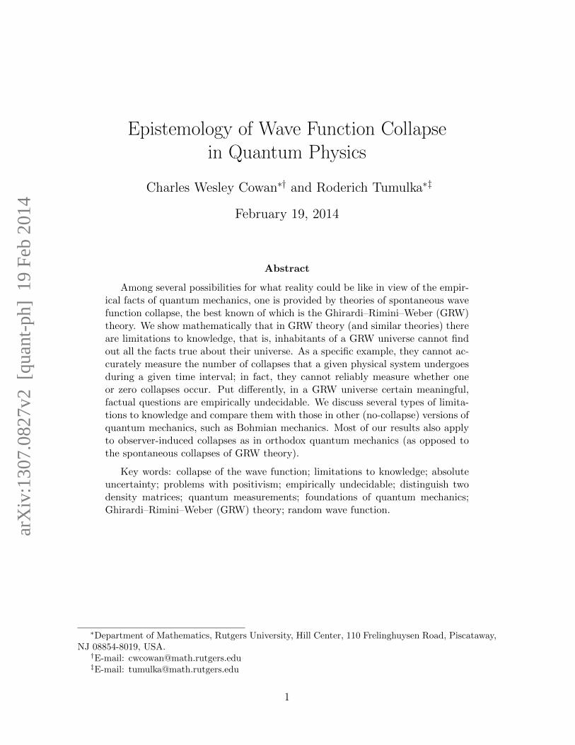
R

maximum

I−| >< |

1

2/3

1/2

0

0 1/2 2/3 1

p

blind guessing

ψ ψ

Figure 1: Reliability of experiments for detecting a collapse of the wave function (17)to one of the two contributions, as a function of p, the probability of collapse. Graphsare shown for blind guessing, for the quantum measurement of E1 = I − |ψ〉〈ψ|, and forthe maximal value of any experiment.

See Figure 1.One can understand easily why the optimal strategy changes at p = 2/3. Suppose

we carry out E1 (corresponding to I − |ψ〉〈ψ|) and obtain outcome Z; as we saw above,if Z = 1 then a collapse must have occurred, and if Z = 0 then the probability that acollapse occurred is p/(2 − p); this value is < 1/2 for p < 2/3 and > 1/2 for p > 2/3.Thus, for p < 2/3 the best retrodiction in case Z = 0 is that no collapse occurred,whereas for p > 2/3 it is better to always answer “yes” in both cases, Z = 1 and Z = 0.

4.2 Other Choices of ψ

The fact that knowledge is limited does not depend on whether the superposition (17)involved two or more contributions, nor on whether the coefficients of the contributionswere equal. Consider an arbitrary initial wave function ψ from the unit sphere S(H )of an n-dimensional Hilbert space H and an orthonormal basis B = {b1, . . . , bn} ofH . Suppose that collapse occurs with probability p and projects ψ to one of the basisvectors with the quantum probability; that is, the final state vector ψ′ has distribution

P(ψ′ = 〈bk|ψ〉

|〈bk|ψ〉|bk)

= |〈bk|ψ〉|2 p , (29)

P(ψ′ = ψ) = 1− p . (30)

16

Then the reliability, which depends on ψ and on the experiment E , is bounded by [13]

Rψ(E ) ≤ 1− p

n∀ψ ∈ S(H ) ∀E ∀p ∈ [0, n

n+1] . (31)

Equality holds for ψ =∑

k n−1/2bk and E the quantum measurement of E = I−|ψ〉〈ψ|.

For other ψ, the optimal reliability Rψ = maxE Rψ(E ) is even less than 1 − p/n; forψ = 2−1/2b1 + 2−1/2b2 it is still Rψ = 1 − p/2. Curiously, for generic ψ the optimalexperiment is different from the quantum measurement of I − |ψ〉〈ψ|; it is still of theform I − |ψ〉〈ψ| but with ψ 6= ψ; we will give more detail around (46) below.

For p > n/(n + 1), no experiment is more reliable than blind guessing (for which(27) is still valid),

Rψ(E ) ≤ p ∀ψ ∈ S(H ) ∀E ∀p ∈ [ nn+1

, 1] . (32)

4.3 Experiments Beginning Before t2

So far we have considered only experiments beginning at t2. One might think that anapparatus might do better that interacts with the system during [t1, t2], for examplebecause it might seem easier to detect a flash when it happens than at a later time.However, as mentioned already at the end of Section 3, when trying to measure theflashes in a system during [t1, t2] we do not want to disturb them; that is, we want them tooccur in the same pattern as they would have occurred without intervention. Of course,in a stochastic theory it is not meaningful to ask after an intervention during [t1, t2]whether the pattern of flashes in [t1, t2] would have been the same had no interventionoccurred. It is meaningful, however, to ask whether the distribution of the flashes wouldhave been the same had no intervention occurred. We now show that the distributionwill in fact be changed by any informative intervention and conclude that an experimentinteracting with the system before t2 will necessarily disturb the flashes during [t1, t2].

The key to showing that the probability distribution of the flashes after the inter-vention is different from what it would have been without intervention is that the wavefunction of the system gets changed by the intervention. Indeed, imagine an experimentEnd (nd stands for “non-disturbing”) that, when applied to a system with a wave func-tion ψ′ as in (18), will return the system undisturbed, with the same wave function ψ′.Then End will not reveal whether a collapse has occurred or not (i.e., whether ψ′ = ψor not), and in fact will yield no information at all about this question; that is, if Z isthe outcome of End and C the number of collapses (i.e., C = 0 if ψ′ = ψ and C = 1otherwise), then the conditional distribution of Z given C does not depend on C,

P(Z = z|C = 0) = P(Z = z|C = 1) (33)

for all z.8

8A slightly stronger statement is true: Suppose that End, when applied to a system with a wavefunction ψ′ that is either |here〉 or |there〉 or ψ as in (17), will return the system undisturbed. ThenEnd will not reveal which state ψ′ is, and in fact will yield no information at all about ψ′; that is, theconditional distribution of Z, given ψ′, does not depend on what ψ′ is, P

(Z = z

∣∣ψ′ = |here〉)

= P(Z =

z∣∣ψ′ = |there〉

)= P

(Z = z

∣∣ψ′ = ψ). This follows from standard quantum measurement theory.

17

Indeed, consider applying End at time t2 repeatedly, N times, to a system with wavefunction ψ′ as in (18) without giving it the possibility to collapse in between. Forc ∈ {0, 1}, let Pz,c = P(Z = z|C = c) with Z the outcome of a single run of End ona system in state ψ′ as in (18). Since the outcomes of the repeated runs of End arestochastically independent, the number of z-occurrences will, conditionally on C = c,have a binomial distribution with parameters N and Pz,c, so that Pz,C can be read offfrom the number of z-occurrences with reliability arbitrarily close to 1, provided thatN is sufficiently large. If, for any z, Pz,1 6= Pz,0 then the value of C could be read offfrom that of Pz,C , so C could be determined as reliably as desired, which contradictsthe bound of Proposition 1. Thus, Pz,1 = Pz,0.

4.4 If ψ is Random

In the previous subsections, we assumed that the initial (i.e., pre-collapse) wave functionψ is known. Now assume that ψ is not known, but random with known probabilitydistribution µ over the unit sphere S(H ). So we have limited information about ψ.Then the reliability of a yes-no experiment E , i.e., the probability that the experimentcorrectly answers whether a collapse has occurred, is easily found to be

Rµ(E ) = EµRψ(E ) =

∫S(H )

µ(dψ)Rψ(E ) . (34)

From (31) and (32), we immediately have that for all µ and all E ,

Rµ(E ) ≤

{1− p

nif 0 ≤ p ≤ n

n+1

p if nn+1≤ p ≤ 1 .

(35)

We also note that Rµ(E ) depends on µ only through ρµ; that is, two distributions withthe same density matrix lead to the same reliability for each experiment, Rµ(E ) = Rρ(E )for ρ = ρµ (see Proposition 9 in Appendix A).9

An extreme case is the uniform distribution u over S(H ), or any distribution µ withdensity matrix ρµ = ρu = 1

nI. For this case we obtain a stronger limitation:

Proposition 3. Let u be the uniform distribution on S(H ). Then

Ru(E ) ≤ max{p, 1− p} (36)

for every experiment E at time t2. That is, no experiment is more reliable than blindguessing. If p = 1

2then, in fact, Ru(E ) = 1/2 for every experiment E at time t2.

We give the proof in Appendix A.

9In fact, the same value Rρ(E ) of reliability applies also when the density matrix ρ arises not from amixture with distribution µ but as the reduced density matrix when the system S under considerationis entangled with another system T , i.e., ρ = trT |ψ〉〈ψ| with ψ the pure state of S and T together [13].

18

Proposition 3 expresses a severe limitation to knowledge: If ψ is uniformly distributedthen the reliability of any experiment is no greater than that of blind guessing. Here isan even stronger statement: If ψ is uniformly distributed then no experiment can conveyany information at all about whether or not a collapse has occurred. More precisely,no experiment on the system can produce an outcome Z such that the conditionaldistribution P(C|Z) would be any different from the a priori distribution (p, 1− p):

Proposition 4. Consider the collapse process as in (29)–(30) and an arbitrary experi-ment E at time t2, possibly with more than two possible outcomes. Let ψ be uniformlydistributed on S(H ). Then P(C = 1|Z) = p and P(C = 0|Z) = 1− p.

4.5 Optimal Way of Distinguishing Two Density Matrices

The problem of distinguishing, at time t2, whether the wave function is collapsed ornot, can be regarded as a special case of the problem of distinguishing two probabilitydistributions µ1, µ2 on S(H ), or of distinguishing two density matrices ρ1, ρ2. Thatis, suppose that a number X ∈ {1, 2} gets chosen randomly with P(X = 1) = p andP(X = 2) = 1−p; as a second step, we are given a system with a random wave functionψ′ chosen according to µX . We can also suppose more directly that, as the second stepin the experiment, we are given a system with density matrix ρX ; this density matrixmay arise from some distribution µX , or from tracing out some other system, or both.Our previous scenario of (29)–(30) corresponds to the special case

µ1 =∑k

|〈bk|ψ〉|2δckbk , ρ1 = diag |ψ〉〈ψ| , (37)

µ2 = δψ , ρ2 = |ψ〉〈ψ| (38)

with ck = 〈bk|ψ〉/|〈bk|ψ〉| and

diagA =∑k

|bk〉〈bk|A|bk〉〈bk| . (39)

We now ask, how well can we retrodict X from experiments on the system? Again,any experiment E with two possible outcomes, 1 and 2, is characterized by a self-adjointoperator 0 ≤ E ≤ I (i.e., one with eigenvalues between 0 and 1), namely E = E1 (so thatE2 = I −E), and the usefulness of E for our purpose can be quantified by its reliabilityR(ρ1, ρ2,E ), i.e., the probability that its outcome Z agrees with X. Using that the maintheorem about POVMs applies also to systems that have a density matrix, rather thana wave function, and then says that the outcome Z has probability distribution

P(Z = z) = tr(ρE) , (40)

19

we find that

R(ρ1, ρ2,E ) = P(Z = 1, X = 1) + P(Z = 2, X = 2) (41)

= P(Z = 1|X = 1)P(X = 1) + P(Z = 2|X = 2)P(X = 2) (42)

= p tr(Eρ1

)+ (1− p) tr

((I − E)ρ2

)(43)

= 1− p+ tr(E(pρ1 − (1− p)ρ2

)). (44)

Note that the reliability depends on E only through E.Which E will maximize the reliability for given ρ1, ρ2, and p?

Proposition 5 (Helstrom [31]). For a given self-adjoint operator A, tr(EA) is maxi-mized among Es with 0 ≤ E ≤ I by those and only those E with

P+(A) ≤ E ≤ P+(A) + P0(A) , (45)

where P+(A) is the projection to the subspace H+(A) spanned by all eigenvectors of Awith positive eigenvalues, and P0(A) is the projection to the eigenspace H0(A) of A witheigenvalue 0. If 0 is not an eigenvalue of A, then P0(A) = 0, and the optimizer E =P+(A) is unique. The maximal value of tr(EA) is the sum of the positive eigenvalues ofA (with multiplicities).

In our case, the projection to H+(pρ1− (1−p)ρ2) is an optimal choice of E, and themaximal reliability is 1 − p plus the sum of all positive eigenvalues of pρ1 − (1 − p)ρ2;this reliability is < 1 unless H+(ρ1) is orthogonal to H+(ρ2).

Coming back to the special case (37)–(38) with known ψ, this optimal E operatorand the maximal reliability can be specified explicitly. For the sake of completeness, wequote the formulas from [13]:

Eoptψ,p =

{I − |ψ〉〈ψ| if 0 < p ≤ n

n+1,

I if nn+1≤ p < 1 ,

(46)

with ψ = M−1ψ/‖M−1ψ‖, M = zψ,pI + diag |ψ〉〈ψ|,

zψ,p = f−1ψ

( p

1− p

)≥ 0 , fψ(z) =

n∑k=1

|ψk|2

z + |ψk|2for z ≥ 0 , (47)

and

Roptψ,p =

{p(1 + zψ,p) if 0 < p ≤ n

n+1,

p if nn+1≤ p < 1 .

(48)

4.6 If ψ is Unknown

Often it is desirable to have an experiment that works for unknown ψ. However, it is notobvious what it should mean for an experiment to work for unknown ψ. One approach,

20

with a Bayesian flavor, would be to take this to mean that the experiment works (i.e.,is more reliable than blind guessing) for random ψ with uniform distribution. We havealready discussed this scenario and can conclude that in this approach it is impossiblefor the inhabitants of a GRWm or GRWf world to measure the collapses.

However, it can be questioned whether an unknown ψ can be assumed to be uniformlydistributed. So here is another approach. Obviously, any experiment E that we choosewill have high reliability for some ψs and low reliability (lower than blind guessing) forother ψs (as the average reliability over all ψ equals that of blind guessing). We maywish to maximize the size of the set

SE ={ψ ∈ S(H ) : Rψ(E ) > max{p, 1− p}

}, (49)

the set of ψs for which E is more reliable than blind guessing. The natural measure of“size” is the (normalized) uniform distribution u on S(H ). There do exist experimentsfor which u(SE ) > 1/2 [14], but we have reason [14] to conjecture that u(SE ) ≤ 1−1/e ≈0.632. If this is right, it is another curious limitation to knowledge: While you can dobetter than blind guessing on more than 50% of all wave functions, you cannot do betterthan blind guessing on more than 64% of all wave functions.

Here are further results concerning u(SE ), expressing limitations to knowledge.

Proposition 6. [14] For p < 1/2− 1/√

8 ≈ 0.146 and p > 1/2 + 1/√

8 ≈ 0.854, all Hand all E , u(SE ) ≤ 1/2.

That is, for p close to 0 or 1, one cannot even do better than blind guessing for amajority of wave functions.

Proposition 7. [14] For H with dim H = 2, all 0 ≤ p ≤ 1 and all E , u(SE ) ≤ 1/2.

5 Measurements of m(x) in GRWm

In this section we investigate the accuracy and reliability of genuine measurements ofm(x) by inhabitants of a GRWm universe. We have shown above that m(x) is notmeasurable with microscopic accuracy. We now show that it is measurable on themacroscopic level. Our analysis can be regarded as an elaboration of statements byGhirardi et al. [23], [5, section 10.2] to the effect that different degrees of “accessibility”of m(x) can occur. Specifically, we confirm that the quantity R(V ) that they intro-duced governs the measurability of m(x): the average of m(x) over V can be measuredaccurately and reliably whenever R(V ) is small.

So consider a coarse-grained, macroscopic version m(x) of m(x), for example

m1(x) = (g` ∗m)(x) =N∑i=1

mi 〈ψ|g`(Qi − x)|ψ〉 (50)

with ∗ convolution, g` the Gaussian function of width ` as in (4), and ` the length scaleof the coarse graining (independent of the GRW length σ), or, based on a partition of

21

R3 into cubes of side length `,

m2(x) =1

`3

∫C(x)

dx′m(x′) , (51)

with C(x) the cube containing x.Here is a simple procedure for a measurement of m(x) (or of m(x) with inaccuracy

`). While this procedure is not practically feasible, it shows the possibility in principleand may suggest more practical schemes if those are desired. We consider a macroscopicsystem of N “particles” with (GRW) wave function ψ(q) = ψ(q1, . . . , qN). Carry outan ideal quantum measurement of the position observables on all N particles, withoutcome Q = (Q1, . . . , QN) distributed with distribution density P(Q = q) = |ψ(q)|2;let the estimator for m(x) be

M(x) =N∑i=1

mi δ3(Qi − x) (52)

or a coarse-grained version M(x) of M(x), for example

M1(x) =N∑i=1

mi g`(Qi − x) (53)

or

M2(x) =1

`3

∫C(x)

dx′M(x′) =1

`3

∑i:Qi∈C(x)

mi . (54)

Put differently, M(x) are the outcomes of a joint ideal quantum measurement of the

commuting observables M(x), the mass density operators as in (11).It follows from (10) that

m(x) = EM(x) and m1,2(x) = EM1,2(x) . (55)

So the estimator will be close to the true value if its variance is small. Specifically,the relative inaccuracy with which m2(x) can be measured in this way is the standard

deviation of M2(x) divided by m2(x), which is exactly Ghirardi’s R(V ) with V = C(x),

R(C(x)) =〈ψ|( 1

`3M(C(x))− m2(x))2|ψ〉1/2

m2(x). (56)

While we do not have a proof that no other method of estimating m2(x) is more accurate,this seems plausible, as no better method comes to mind.

Obviously, the inaccuracy (56) depends on the wave function ψ. This leads us tothe question, for typical wave functions arising from the GRW process, how large dowe have to choose ` to make the inaccuracy R(C(x)) smaller than, say, 10%? Let usconsider a few examples.

22

An object of macroscopic size consisting of a uniform solid or liquid at everydayconditions has interatomic distances of 10−10 to 10−9 m, and we may expect the wavefunction of the nucleus to be spread out over similar distances (except for permutationsymmetry). Since, for ` = 3 × 10−9 m, a volume of `3 contains 30 to 3 × 104 atoms,

M2(x) involves an average over many atoms; thus, for this size of ` or larger, we mayexpect the variation of the wave function (such as the ground state of the solid) to have

little effect on M2(x), and R(C(x)) to be small.Now consider a solid object O of size δ (or even a sheet of thickness δ, since only 1

dimension of space is relevant), an ` > δ, and a ψ that is a superposition of two differentpositions of O with a difference greater than `. Then one term in the superposition maycorrespond to O lying entirely in C(x), while the other term corresponds to O lyingentirely outside of C(x). Let the coefficients of the terms be c1 and c0, respectively; then,

for a suitable constant m0, M2(x), if measured, equals m0 with probability p = |c1|2 andequals 0 with probability q = |c2|2 = 1 − |c1|2. It follows that m2(x) = pm0, that the

standard deviation of M2(x) is m0√pq, and that R(C(x)) =

√q/p, which is greater

than 10% for every p < 99%. Thus, except for extreme values of p, such a superpositionyields quite a large value of R(C(x)), and thus probably low accuracy as a genuinemeasurement of m2(x). However, since superpositions of different locations more thanσ apart are suppressed by the spontaneous collapses, such wave functions are unlikelyto occur for ` � σ = 10−7 m. Or rather, they cannot persist much longer than for∆t = 1/Nλ.

These considerations suggest that m(x) can usually be measured with small relativeinaccuracy and high reliability at a spatial and temporal resolution of

∆x = 10−7 m , ∆t =1

N∆xλ, (57)

where N∆x is the number of nucleons in the volume (∆x)3. On the other hand, examplescan be set up, at least artificial ones, for which these estimates are not valid: if ψ = ϕ⊗N

with ϕ a 1-particle wave function that is spread out over distances much greater than σ,and if the N particles do not interact (say, H = 0), then the spontaneous collapses arenot efficient at localizing the wave function, and R(C(x)) will not become small untilafter 108 years (when almost every particle has been hit by a collapse).

A Proofs

Proposition 8. If µ1 6= µ2 are distributions of wave functions with equal density matri-ces ρµ1 = ρµ2 then no experiment can distinguish between an ensemble of wave functionswith distribution µ1 and one with µ2.

Proof. This is a consequence of the main theorem about POVMs (14). If E is carriedout on an ensemble of systems with wave functions ψ ∈ S(Hsys) distributed accordingto µ1 then the probability of obtaining outcome z is

P(Z = z) = tr(E(z)ρµ1

), (58)

23

so it depends on µ1 only through ρµ1 . Thus, since ρµ2 = ρµ1 , the distribution of outcomeswould be the same in an ensemble distributed according to µ2.

Proposition 9. Consider the collapse process as in (29)–(30) and arbitrary E . Let Ezbe the POVM associated with E by the main theorem about POVMs, and E = Eyes.Then

Rψ(E ) = 〈ψ|A|ψ〉 (59)

withA = p diagE + (1− p)(I − E) (60)

and diag the “diagonal part” as defined in (39). For ψ as in (17), Rψ(E1) = 1 − p/2(i.e., Eq. (25) holds). For random ψ with distribution µ,

Rµ(E ) = tr(ρµA) . (61)

Proof. We have that

P(Z = yes|C = 0) = 〈ψ|E|ψ〉 (62)

P(Z = yes|C = 1) =∑k

∣∣〈bk|ψ〉∣∣2 〈bk|E|bk〉 (63)

= 〈ψ| diagE|ψ〉 . (64)

Now (59) follows, together with (25) and (61); (25) is obtained as the special case withψ = 2−1/2(b1 + b2) and E = I − |ψ〉〈ψ|.

Proposition 3. Let u be the uniform distribution on S(H ). Then Ru(E ) ≤ max{p, 1−p} for every experiment E at time t2. If p = 1

2then, in fact, Ru(E ) = 1/2 for every

experiment E at time t2.

Proof. By (61),

Ru(E ) =1

ntrA =

p

ntrE +

1− pn

tr(I − E) = 1− p− 1− 2p

ntrE . (65)

Note that 0 ≤ E ≤ I and thus 0 ≤ trE ≤ n. For 0 ≤ p ≤ 1/2, (65) is ≤ 1 − p sincetrE ≥ 0 and 1− 2p ≥ 0. For 1/2 < p ≤ 1, rewrite (65) as

Ru(E ) = p− 2p− 1

ntr(I − E) , (66)

note tr(I − E) ≥ 0 and 2p− 1 ≥ 0, and conclude Ru(E ) ≤ p.

Proposition 4. Consider the collapse process as in (29)–(30) and an arbitrary experi-ment E at time t2, possibly with more than two possible outcomes. Let ψ be uniformlydistributed on S(H ). Then P(C = 1|Z) = p and P(C = 0|Z) = 1− p.

24

Proof. Let Ez be the POVM of E ; then

P(C = 1|Z = z) =P(Z = z|C = 1)P(C = 1)

P(Z = z|C = 0)P(C = 0) + P(Z = z|C = 1)P(C = 1)(67)

=tr(ρ diagEz)p

tr(ρEz)(1− p) + tr(ρ diagEz)p= p (68)

using ρ = 1nI.

Acknowledgments. We thank Sheldon Goldstein for helpful discussions. Both authorsare supported in part by NSF Grant SES-0957568. R.T. is supported in part by grantno. 37433 from the John Templeton Foundation and by the Trustees Research FellowshipProgram at Rutgers, the State University of New Jersey.

References

[1] V. Allori: Primitive Ontology and the Structure of Fundamental Physical Theo-ries. Pages 58–75 in D. Z. Albert and A. Ney (ed.s): The Wave Function, OxfordUniversity Press (2013)

[2] V. Allori: On the Metaphysics of Quantum Mechanics. Pages 116–140 in S. LeBihan(ed.): Precis de philosophie de la physique, Vuibert (2013)

[3] V. Allori, S. Goldstein, R. Tumulka, N. Zanghı: On the Common Structure ofBohmian Mechanics and the Ghirardi–Rimini–Weber Theory. British Journal forthe Philosophy of Science 59: 353–389 (2008). http://arxiv.org/abs/quant-ph/0603027

[4] V. Allori, S. Goldstein, R. Tumulka, N. Zanghı: Many-Worlds and Schrodinger’sFirst Theory. British Journal for the Philosophy of Science 62(1): 1–27 (2011).http://arxiv.org/abs/0903.2211

[5] A. Bassi, G.C. Ghirardi: Dynamical Reduction Models. Physics Reports 379: 257–426 (2003). http://arxiv.org/abs/quant-ph/0302164

[6] A. Bassi, G.C. Ghirardi, D.G.M. Salvetti: The Hilbert space operator formalismwithin dynamical reduction models. Journal of Physics A: Mathematical and The-oretical 40: 13755–13772 (2007). http://arxiv.org/abs/0707.2940

[7] J. S. Bell: De Broglie–Bohm, Delayed-Choice Double-Slit Experiment, and Den-sity Matrix. International Journal of Quantum Chemistry 14: 155–159 (1980).Reprinted as chapter 14 of [9].

25

[8] J. S. Bell: Are There Quantum Jumps? Pages 41–52 in C. W. Kilmister (ed.)Schrodinger. Centenary Celebration of a Polymath. Cambridge University Press(1987). Reprinted as chapter 22 of [9].

[9] J. S. Bell: Speakable and Unspeakable in Quantum Mechanics. Cambridge Univer-sity Press (1987)

[10] F. Benatti, G.C. Ghirardi, R. Grassi: Describing the macroscopic world: closing thecircle within the dynamical reduction program. Foundations of Physics 25: 5–38(1995)

[11] D. Bohm: A Suggested Interpretation of the Quantum Theory in Terms of “Hidden”Variables, I and II. Physical Review 85: 166–193 (1952)

[12] S. Colin, T. Durt, R. Tumulka: On Superselection Rules in Bohm–Bell Theories. J.Phys. A: Math. Gen. 39: 15403–15419 (2006). http://arxiv.org/abs/quant-ph/0509177

[13] C. W. Cowan, R. Tumulka: Can One Detect Whether a Wave Function Has Col-lapsed? Preprint (2013) http://arxiv.org/abs/1307.0810

[14] C. W. Cowan, R. Tumulka: Detecting Wave Function Collapse Without PriorKnowledge. Preprint (2013) http://arxiv.org/abs/1312.7321

[15] E. Deotto, G.C. Ghirardi: Bohmian Mechanics Revisited. Foundations of Physics28: 1–30 (1998). http://arxiv.org/abs/quant-ph/9704021

[16] L. Diosi: Models for universal reduction of macroscopic quantum fluctuations. Phys.Rev. A 40: 1165–1174 (1989)

[17] D. Durr, S. Goldstein, N. Zanghı: Quantum Equilibrium and the Origin of AbsoluteUncertainty. Journal of Statistical Physics 67: 843–907 (1992). http://arxiv.

org/abs/quant-ph/0308039

[18] D. Durr, S. Goldstein, N. Zanghı: Quantum Equilibrium and the Role of Operatorsas Observables in Quantum Theory. Journal of Statistical Physics 116: 959–1055(2004). http://arxiv.org/abs/quant-ph/0308038

[19] D. Durr, S. Goldstein, N. Zanghı: On the Weak Measurement of Velocity inBohmian Mechanics. Journal of Statistical Physics 134: 1023–1032 (2009). http://arxiv.org/abs/0808.3324

[20] A. Einstein, orally during W. Heisenberg’s 1926 lecture at Berlin; later related byHeisenberg, quoted in [37].

[21] H. Everett: Relative State Formulation of Quantum Mechanics. Review of ModernPhysics 29: 454–462 (1957)

26

[22] G.C. Ghirardi: Collapse Theories. In E. N. Zalta (ed.), Stanford Encyclopediaof Philosophy, published online by Stanford University (2007). http://plato.

stanford.edu/entries/qm-collapse

[23] G.C. Ghirardi, R. Grassi: Bohm’s Theory versus Dynamical Reduction. Pages 353–377 in J. T. Cushing et al. (ed.s): Bohmian Mechanics and Quantum Theory: AnAppraisal. Dordrecht: Kluwer (1996)

[24] G.C. Ghirardi, A. Rimini, T. Weber: Unified Dynamics for Microscopic and Macro-scopic Systems. Physical Review D 34: 470–491 (1986)

[25] K. Godel: Uber formal unentscheidbare Satze der Principia Mathematica und ver-wandter Systeme I. Monatshefte fur Mathematik und Physik 38: 173–198 (1931)

[26] S. Goldstein: Stochastic Mechanics and Quantum Theory. Journal of StatisticalPhyics 47: 645–667 (1987)

[27] S. Goldstein: Quantum Theory Without Observers. Physics Today, Part One:March 1998, 42–46. Part Two: April 1998, 38–42.

[28] S. Goldstein: Bohmian Mechanics. In E. N. Zalta (ed.), Stanford Encyclopediaof Philosophy, published online by Stanford University (2001). http://plato.

stanford.edu/entries/qm-bohm

[29] S. Goldstein, J. Taylor, R. Tumulka, N. Zanghı: Are All Particles Real? Studiesin History and Philosophy of Modern Physics 36: 103–112 (2005). http://arxiv.org/abs/quant-ph/0404134

[30] S. Goldstein, R. Tumulka, N. Zanghı: The Quantum Formalism and the GRWFormalism. Journal of Statistical Physics 149: 142–201 (2012). http://arxiv.

org/abs/0710.0885

[31] C. W. Helstrom: Quantum Detection and Estimation Theory. New York: AcademicPress (1976)

[32] T. Maudlin: Can the world be only wavefunction? Pages 121–143 in S. Saunders, J.Barrett, A. Kent, and D. Wallace (ed.s): Many Worlds? Everett, Quantum Theory,and Reality, Oxford University Press (2010)

[33] B. Monton: Wave Function Ontology. Synthese 130: 265–277 (2002)

[34] B. Monton: The Problem of Ontology for Spontaneous Collapse Theories. Studiesin History and Philosophy of Modern Physics 35: 407–421 (2004)

[35] E. Nelson: Quantum Fluctuations. Princeton University Press (1985)

[36] P. Pearle: Combining stochastic dynamical state-vector reduction with spontaneouslocalization. Physical Review A 39: 2277–2289 (1989)

27

[37] A. Salam: Unification of Fundamental Forces. Cambridge University Press (1990)

[38] R. Tumulka: A Relativistic Version of the Ghirardi–Rimini–Weber Model. Journalof Statistical Physics 125: 821–840 (2006). http://arxiv.org/abs/quant-ph/

0406094

[39] R. Tumulka: The Point Processes of the GRW Theory of Wave Function Collapse.Reviews in Mathematical Physics 21: 155–227 (2009). http://arxiv.org/abs/

0711.0035

[40] L. Vaidman: Many-Worlds Interpretation of Quantum Mechanics. In E. N. Zalta(ed.), Stanford Encyclopedia of Philosophy, published online by Stanford University(2002). http://plato.stanford.edu/entries/qm-manyworlds

28