LUND UNIVERSITY

PO Box 117221 00 Lund+46 46-222 00 00

Environmental optimization in fractionating industrial wastes using cost-benefitanalysis

Stenis, Jan

Published in:Resources, Conservation & Recycling

DOI:10.1016/j.resconrec.2003.09.005

2004

Link to publication

Citation for published version (APA):Stenis, J. (2004). Environmental optimization in fractionating industrial wastes using cost-benefit analysis.Resources, Conservation & Recycling, 41(2), 147-164. https://doi.org/10.1016/j.resconrec.2003.09.005

Total number of authors:1

General rightsUnless other specific re-use rights are stated the following general rights apply:Copyright and moral rights for the publications made accessible in the public portal are retained by the authorsand/or other copyright owners and it is a condition of accessing publications that users recognise and abide by thelegal requirements associated with these rights. • Users may download and print one copy of any publication from the public portal for the purpose of private studyor research. • You may not further distribute the material or use it for any profit-making activity or commercial gain • You may freely distribute the URL identifying the publication in the public portal

Read more about Creative commons licenses: https://creativecommons.org/licenses/Take down policyIf you believe that this document breaches copyright please contact us providing details, and we will removeaccess to the work immediately and investigate your claim.

Appendix 1. Paper I

Environmental Optimisation in Fractionating Industrial Wastes

Using Cost-Benefit Analysis

Reprinted from

Resources, Conservation and Recycling 2004;41(2):147-164

with permission from Elsevier.

© 2003 Elsevier B. V. All rights reserved.

Environmental Optimisation in Fractionating Industrial Wastes

Using Cost-Benefit Analysis

Resources, Conservation and Recycling 2004;41(2):147-164

© 2003 Elsevier B. V. All rights reserved.

Jan Stenis1

Department of Construction and Architecture, Lund University,

P.O. Box 118, SE-221 00 Lund, Sweden

___________________________________________________________________________

Abstract This paper proposes that industrial waste be regarded, in a business economic sense, as having the same basic status as regular products. A basic mathematical expression for assigning industrial costs to waste is presented. The expression can be employed in conjunction with cost-benefit analysis for estimating the “true” internal costs of industrial waste. In two case studies presented, industrial waste was found to have a substantial negative impact on profits. This is seen as a possibly unavoidable consequence of industrial companies’ acting in accordance with the ideal of improving the sustainability and productivity of resource use. ___________________________________________________________________________ Key words: Integrated industrial waste management, waste fractionating optimisation, cost-benefit analysis. ___________________________________________________________________________

1 Corresponding author. E-mail address: jan.stenis@bekon.lth.se, Tel.: +46 46 222 7343, Fax: +46 46 222 4414, Correspondence address: Jan Stenis, Department of Construction and Architecture, Lund Institute of Technology, Lund University, P.O. Box 118, SE-221 00 Lund, Sweden.

1. Introduction The disposal of industrial waste often creates serious environmental problems. In the long run, these problems must be eliminated, or considerably reduced, to conserve the natural environment. This calls for the identification of links between company profit, as expressed in consolidated profit and loss accounts, and both the avoidance and proper handling of waste. Thus, a new way of regarding waste, or a shift in paradigm, is called for. The paradigm proposed here involves equating industrial waste with regular products in terms of the allocation of costs, an approach that will be termed the equality principle. A theoretical framework upon which such a principle, directed at sustainable development, can be based is presented here. In a practical sense, optimizing the management of industrial waste involves the optimization of waste fractionation. It is generally accepted that the cost of waste fractionation increases in proportion to the number of fractions into which waste is separated (e.g. Asplund et al., 1994). A method of optimizing the number and kinds of waste to be separated provides a sound economic basis for designing an environmentally friendly waste management system. The optimization of fractionation with regard to economics is seldom dealt with in the literature, which instead focuses on indicators used in making financial assessments of fractionation, often in connection with the purchase of equipment for fractionation. Among the methods employed in identifying such indicators are the Net Present Value (NPV) method, the Internal Rate of Return (IRR) method, the Return On Investment (ROI) method and the Payback method (Horngren et al., 1993). In the first of these, the NPV method, a project’s net present value is the sum of the cash flows involved, each discounted to its current value. The project with the highest positive NPV is then the most appropriate. In the IRR method, the discount rate that equates the current value of the project’s expected cash inflow to the current value of the project’s expected costs is calculated. The project exhibiting the highest internal rate of return is considered to be the best, provided the current IRR is higher than the cost of the capital required to finance the project. In the ROI method, the return on investment is calculated as the income (or profit) divided by the investment required to obtain the income or profit in question; the higher the ROI, the more attractive the project is considered to be. Finally, in the Payback method, the number of years predicted to be required to recover the original investment in the project is calculated, and naturally, the shorter the period, the better. Since the length of the payback period provides an estimate of how long funds will be tied up in the project, it is often used as an indicator of a project’s liquidity (Freeman (Ed.), 1995). A more output-related waste management approach is that based on the concept of joint production. When the product and the waste are produced jointly in one and the same process, linear programming is used to calculate the optimal output proportions. Two other approaches employed to determine such matters as the best location and size of a facility, and the optimal timing of waste allocation, are linear programming (as a basic method and not simply a tool as in the case mentioned above) and simulation (Barlishen and Baetz, 1996).

Methods of optimization based on cost-benefit theory, although clearly applicable in a waste management context, are rarely employed, in theoretical studies or in practice. An informal survey carried out by the author, directed primarily at large manufacturing companies in Sweden, provided conclusive evidence of this. The present paper aims to show how cost-benefit methods can be applied in terms of the equality principle so as to provide environmental management guidelines concerning product cost and investment assessments, influencing both consolidated profit and loss accounts and budgets for external use. A number of methods traditionally used in industry to estimate product costs are reviewed. Examples are also given of how these methods can be modified to obtain estimates of the “true” internal costs of industrial waste fractions considered here through the use of the equality principle. Two case studies are presented. These deal with the applicability of this principle to two fairly typical industrial scenarios concerned with the manufacture of real products by existing companies: (A) a company manufacturing a very limited number of bulk products, largely produced from the same type of raw materials, and (B) a company manufacturing many different products, most of them mechanically complicated. The modified product cost estimation methods considered are applied to the two scenarios. On the basis of both the theoretical and the practical parts of the paper, conclusions are drawn regarding the suitability of using the suggested modifications of traditional estimation methods as a general cost-benefit theory for industrial waste management, with the aim of achieving and maintaining a sustainable development.

2. Basic rationale Application of the methods described above involves considering different scenarios. A particular waste fraction is studied within a given production scenario, involving a number of waste fractions with which various revenues and costs are associated. The profitability of a given waste fraction is then used as input in assessing the waste fraction shadow price, leading to an environmental improvement incentive. In general terms, a shadow price represents the true marginal value of a product or the opportunity cost of a resource, both of which may differ from the market price. The idea of using a shadow price here is that if companies were actually charged the shadow price associated with waste of a particular type, they would adjust to this, resulting in the desired environmental standard being met. In any given scenario, therefore, a new separate assessment of revenues and costs is required for each fraction considered. The costs and revenues are estimated in the manner described below. In the next section, various methods commonly used for estimating product costs, and ways in which these methods can be adopted for the estimation of the “true” internal costs of waste fractionation, are presented. The aim is to allocate costs to the waste produced, with the ultimate aim of improving the environment. The underlying assumption is that from a business point of view a given waste fraction can be regarded as a company product, one that should contribute to bearing the company’s costs, just as regular products do. If it fails to do this, financial losses result, which must be covered by surplus profit from other activities in the company. Ideally, no waste should arise from the industrial production process. Since this is not practically possible, waste must be minimized and be transformed into products that are profitable. If this can be accomplished, problems associated with waste will largely disappear. This view is consistent with various developments in Sweden, for example, the governmental

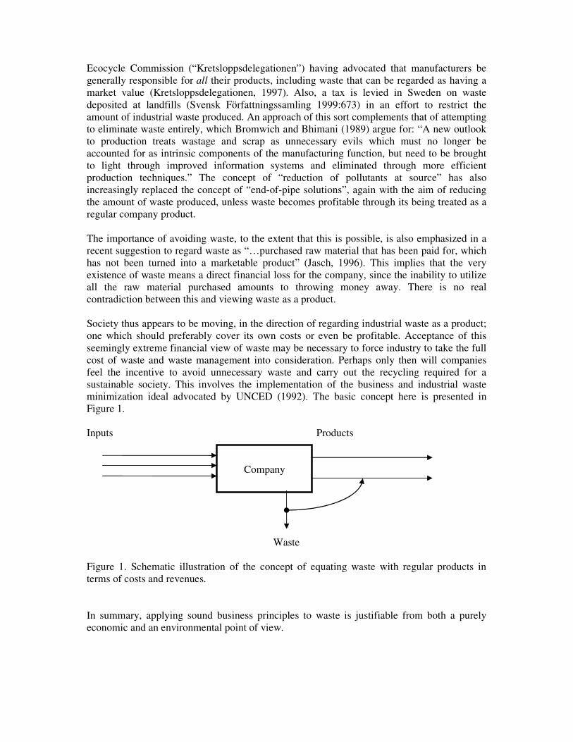
Ecocycle Commission (“Kretsloppsdelegationen”) having advocated that manufacturers be generally responsible for all their products, including waste that can be regarded as having a market value (Kretsloppsdelegationen, 1997). Also, a tax is levied in Sweden on waste deposited at landfills (Svensk Författningssamling 1999:673) in an effort to restrict the amount of industrial waste produced. An approach of this sort complements that of attempting to eliminate waste entirely, which Bromwich and Bhimani (1989) argue for: “A new outlook to production treats wastage and scrap as unnecessary evils which must no longer be accounted for as intrinsic components of the manufacturing function, but need to be brought to light through improved information systems and eliminated through more efficient production techniques.” The concept of “reduction of pollutants at source” has also increasingly replaced the concept of “end-of-pipe solutions”, again with the aim of reducing the amount of waste produced, unless waste becomes profitable through its being treated as a regular company product. The importance of avoiding waste, to the extent that this is possible, is also emphasized in a recent suggestion to regard waste as “…purchased raw material that has been paid for, which has not been turned into a marketable product” (Jasch, 1996). This implies that the very existence of waste means a direct financial loss for the company, since the inability to utilize all the raw material purchased amounts to throwing money away. There is no real contradiction between this and viewing waste as a product. Society thus appears to be moving, in the direction of regarding industrial waste as a product; one which should preferably cover its own costs or even be profitable. Acceptance of this seemingly extreme financial view of waste may be necessary to force industry to take the full cost of waste and waste management into consideration. Perhaps only then will companies feel the incentive to avoid unnecessary waste and carry out the recycling required for a sustainable society. This involves the implementation of the business and industrial waste minimization ideal advocated by UNCED (1992). The basic concept here is presented in Figure 1.

Inputs Products

Company

Waste

Figure 1. Schematic illustration of the concept of equating waste with regular products in terms of costs and revenues.

In summary, applying sound business principles to waste is justifiable from both a purely economic and an environmental point of view.

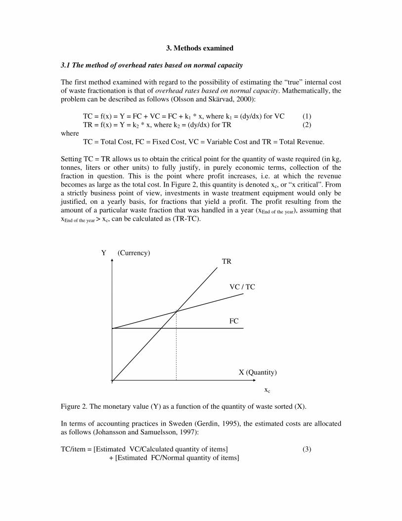
3. Methods examined 3.1 The method of overhead rates based on normal capacity The first method examined with regard to the possibility of estimating the “true” internal cost of waste fractionation is that of overhead rates based on normal capacity. Mathematically, the problem can be described as follows (Olsson and Skärvad, 2000):

TC = f(x) = Y = FC + VC = FC + k1 * x, where k1 = (dy/dx) for VC (1) TR = f(x) = Y = k2 * x, where k2 = (dy/dx) for TR (2)

where TC = Total Cost, FC = Fixed Cost, VC = Variable Cost and TR = Total Revenue.

Setting TC = TR allows us to obtain the critical point for the quantity of waste required (in kg, tonnes, liters or other units) to fully justify, in purely economic terms, collection of the fraction in question. This is the point where profit increases, i.e. at which the revenue becomes as large as the total cost. In Figure 2, this quantity is denoted xc, or “x critical”. From a strictly business point of view, investments in waste treatment equipment would only be justified, on a yearly basis, for fractions that yield a profit. The profit resulting from the amount of a particular waste fraction that was handled in a year (xEnd of the year), assuming that xEnd of the year > xc, can be calculated as (TR-TC). Y (Currency) TR VC / TC FC X (Quantity) xc Figure 2. The monetary value (Y) as a function of the quantity of waste sorted (X).

In terms of accounting practices in Sweden (Gerdin, 1995), the estimated costs are allocated as follows (Johansson and Samuelsson, 1997): TC/item = [Estimated VC/Calculated quantity of items] (3)

+ [Estimated FC/Normal quantity of items]

This estimation method is particularly useful when applied to companies that, for the most part, produce only one kind of product (Olsson and Skärvad, 2000). A major advantage of estimating the normal cost is that it eliminates the influence of the company’s current level of production, since the FC is always distributed over the quantity that is normally produced, regardless of the current level of production (Johansson and Samuelsson, 1997). The FC is sometimes difficult to define since it may not be clear which part of the total FC should be allocated to a particular waste fraction. It may be a question of splitting the total FC into parts representing different types of waste. The most natural FC to be allocated to a waste fraction is that for the annual depreciation of equipment and machinery used to separate that fraction. Apart from this, the FC can consist of factors such as interest, depreciation, rent for facilities and the cost of electric or other types of power, for the time period in question. Wages are usually considered as fixed costs and should thus be apportioned between the waste fractions, for example, in relation to the weight or the volume of the waste fraction considered, the quantity of raw materials employed or the time involved in producing the waste fraction of interest under normal conditions. As already indicated, the waste fractions studied are regarded as a kind of company output. This involves adding the sum of the quantities of the different types of waste associated with a given scenario, to the normal output in the denominator of expression (4) given below. This expression is used to allocate costs to a particular fraction through multiplication either by the total FC, so as to obtain the FC for the waste fraction in question, or by the second term appearing in (3), so as to obtain the FC per item or unit of the waste fraction considered. In this context, it is not unusual for the FC to increase stepwise as the quantity of waste increases, rather than as a straight line as in Figure 2 (Johansson and Samuelsson, 1997). Such a relationship, if found, should be taken into account. Quantity of the waste fraction in question produced (4) Quantity of normal output Sum of the quantities of all

of regular products different waste fractions considered It is necessary to define a suitable production or administrative unit to which expression (4) is to be applied. This may be the entire company, separate divisions or workshops, individual machines, etc. The VC of a particular waste fraction that is separated depends on the following factors in particular: the amount of manpower or handling time required to collect the waste fraction in question, the cost of the raw materials and the energy used in the production process in which the waste is produced, and the cost of ridding the company of the waste material. If the VC directly associated with a given fraction is known, this cost should of course be used. If not, costs can be allocated, just as they were above for the FC, in proportion to the weight or volume of the waste fraction considered, or the amount of raw material used or the time required to produce it. Mathematically, allocation is achieved by multiplying expression (4) by the first term in expression (3). In this case k1 is obtained by dividing the estimated total cost of the waste fraction produced during the year in question by the total amount of this waste fraction produced (in kg, tonnes, litres, etc.), in the production or administration unit being studied. It is not unusual, due to economies of scale, for the VC to either increase or decrease progressively (more commonly the latter) as the quantity referred to increases (see e.g. Johansson and Samuelson, 1997). If such is found to be the case, this should be taken into account.

The TR for a given waste fraction is a function of factors such as the following: the selling price of the waste, the value of reusing or recycling it, the value of the energy extracted if it is incinerated, i.e. a saving in energy that must otherwise be purchased externally, the saving of fuel, and the avoidance of taxes and/or fees levied on landfilling the waste. If the TR for a particular fraction is known, this should, of course, be used. If it is not, either k2 should be calculated in a manner similar to that for k1 above, using expression (4), or the estimated total income arising from the waste fraction in question should be divided by the amount of the waste fraction produced during the time period in question. It should be noted that the separation of a particular waste fraction from one or more other fractions can lead to either an increase or a decrease in the value of one or more of the fractions. For example, if a fraction consists of 50% aluminium and 50% stainless steel, their being separated increases the value of each. The same is true for hazardous waste which, when mixed with other waste, which it contaminates, reduces the possibility of commercially exploiting the other waste. The cost and the income connected with the separation of a given waste fraction depend, therefore, on the fractions it is separated from. A strictly mathematical approach to the problem of mixed waste is to determine the proportions of the various components of the waste mixture and to multiply these proportions by the value per unit of each of the fractions involved, and to also take into account specific separation costs, such as those for the waste separation machinery required and for wages. The usefulness of the overall approach described above is probably greatest in companies that mainly produce homogeneous bulk goods of different kinds, yielding wastes which, for the most part, stem from the same type of raw material. Such is the case for paper mills, brickyards and dairies, for example. In a company producing many different kinds of goods, the waste from producing goods of one type may deviate markedly from those from that arising from the production of goods of another type, in terms of either the relative cost of treating the waste, the revenue provided by the waste, or both. In such cases the approach of employing overhead rates that apply under conditions of normal capacity should be used with the utmost caution, or not at all! 3.2 The average cost estimation method Another approach, that can be used when considering a company producing one product only, is to simply divide the total cost for the period in question by the total production during that period, resulting in the cost per ton, or litre etc. However, this average cost estimation method has certain shortcomings. The fixed and variable costs are not separated, so it is impossible to include the effects of the level of production activity. If the level of production is sub normal, the estimated cost per unit of waste produced will be higher than if the level of production were normal. Hence, when a long-term decision is required, the costs that apply to a normal level of production should be used (Olsson and Skärvad, 2000). In making estimates such as those described above, it may well happen that the quantity of waste sorted (the x-value) falls short of the minimum quantity required (xc), indicating that the collection and sorting of waste will result in a net financial loss. It may, nevertheless, be necessary to collect the waste and separate the fraction in question, when, for example national environmental regulations require this. Alternative justification for collecting and separating waste, despite the loss incurred, is to regard the financial loss as the value of the goodwill the company may receive for showing responsibility in collecting and sorting its waste. The total loss, or the goodwill involved, can be calculated mathematically as the

absolute value of (TR-TC) for the amount of the waste fraction handled during the year of interest (xEnd of the year), assuming that xEnd of the year < xc. When applying the average cost estimation method, the cost of a given waste fraction is determined by multiplying expression (4) by the actual or budgeted average cost for the period in question. However, this will result simply in a cost of the waste per unit of the current total amount of waste in question. 3.3 The equivalent method of cost estimation The third method to be considered in connection with the separation of waste fractions is the equivalent method of cost estimation, used here in a somewhat modified form. This method can be applied to companies producing a limited number of different products, all based on essentially the same raw material and involving similar manufacturing procedures. This is the case in ironworks, spinning mills and weaving mills, for example. Costs are then allocated on the basis of equivalent rates calculated for normal production conditions, normal cost levels and a normal mix of products. The equivalent rates indicate relationships between the costs of the different products. Calculation of the equivalent rate for a particular product during a given period is carried out in accordance with expression (5) (Johansson and Samuelson, 1997).

(Normal cost per unit for a given product) / (Normal cost per unit for the product with the lowest cost per unit) (5)

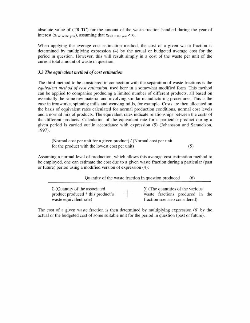
Assuming a normal level of production, which allows this average cost estimation method to be employed, one can estimate the cost due to a given waste fraction during a particular (past or future) period using a modified version of expression (4): Quantity of the waste fraction in question produced (6)

Σ (Quantity of the associated � (The quantities of the various product produced * this product’s waste fractions produced in the waste equivalent rate) fraction scenario considered)

The cost of a given waste fraction is then determined by multiplying expression (6) by the actual or the budgeted cost of some suitable unit for the period in question (past or future).

3.4 The absorption costing method The fourth method of estimation to be considered in connection with the separation of waste fractions is the absorption costing method, also used here in a somewhat modified fashion. This method involves a step-by-step analysis of the contribution of the separate costs to the final cost units, taking into account the following:

• the distribution of direct costs in the final cost units • the distribution of indirect (overhead) costs in the sub-organizations involved (such

as departments) • the distribution of the costs of the sub-organizations involved in the final cost units.

The direct costs usually include the following:

• direct material costs (DM) • direct labor costs (DL) • special direct manufacturing costs, such as patent costs • special selling costs, such as commissions

Indirect costs are usually divided into the following four major categories:

• material overhead costs (MO), such as those for storage, and the wages of the store and purchasing staff

• production overhead costs (PO), such as those for the salaries of the planning and design department staff and for the depreciation of machines and buildings

• administrative overhead costs (AO), such as those for central management and for the financial and personnel departments

• sales overhead costs (SO), such as the salaries of sales management personnel and of salesmen (excluding commissions), and costs for PR.

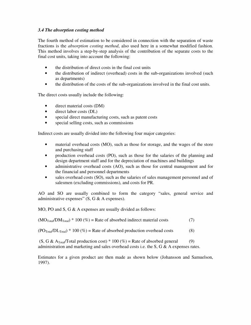
AO and SO are usually combined to form the category “sales, general service and administrative expenses” (S, G & A expenses). MO, PO and S, G & A expenses are usually divided as follows: (MOTotal/DMTotal) * 100 (%) = Rate of absorbed indirect material costs (7) (POTotal/DLTotal) * 100 (%) = Rate of absorbed production overhead costs (8) (S, G & ATotal/Total production cost) * 100 (%) = Rate of absorbed general (9) administration and marketing and sales overhead costs i.e. the S, G & A expenses rates. Estimates for a given product are then made as shown below (Johansson and Samuelson, 1997).

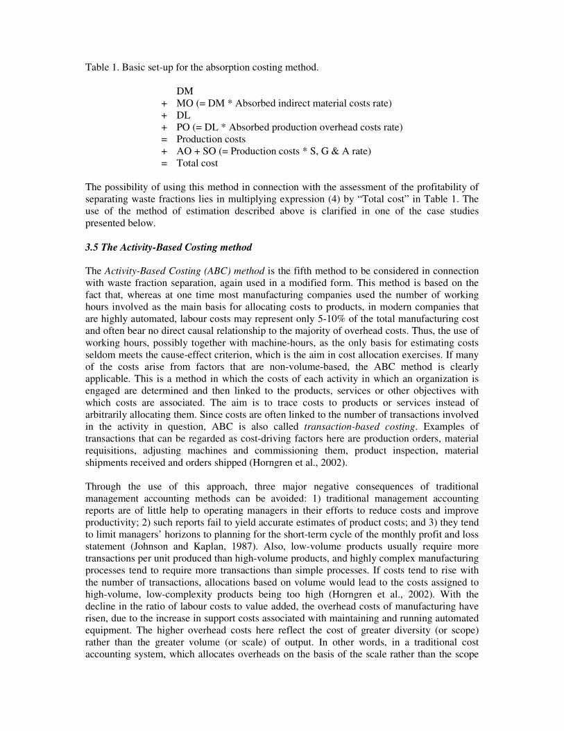
Table 1. Basic set-up for the absorption costing method.

DM + MO (= DM * Absorbed indirect material costs rate) + DL + PO (= DL * Absorbed production overhead costs rate) = Production costs + AO + SO (= Production costs * S, G & A rate) = Total cost

The possibility of using this method in connection with the assessment of the profitability of separating waste fractions lies in multiplying expression (4) by “Total cost” in Table 1. The use of the method of estimation described above is clarified in one of the case studies presented below. 3.5 The Activity-Based Costing method The Activity-Based Costing (ABC) method is the fifth method to be considered in connection with waste fraction separation, again used in a modified form. This method is based on the fact that, whereas at one time most manufacturing companies used the number of working hours involved as the main basis for allocating costs to products, in modern companies that are highly automated, labour costs may represent only 5-10% of the total manufacturing cost and often bear no direct causal relationship to the majority of overhead costs. Thus, the use of working hours, possibly together with machine-hours, as the only basis for estimating costs seldom meets the cause-effect criterion, which is the aim in cost allocation exercises. If many of the costs arise from factors that are non-volume-based, the ABC method is clearly applicable. This is a method in which the costs of each activity in which an organization is engaged are determined and then linked to the products, services or other objectives with which costs are associated. The aim is to trace costs to products or services instead of arbitrarily allocating them. Since costs are often linked to the number of transactions involved in the activity in question, ABC is also called transaction-based costing. Examples of transactions that can be regarded as cost-driving factors here are production orders, material requisitions, adjusting machines and commissioning them, product inspection, material shipments received and orders shipped (Horngren et al., 2002). Through the use of this approach, three major negative consequences of traditional management accounting methods can be avoided: 1) traditional management accounting reports are of little help to operating managers in their efforts to reduce costs and improve productivity; 2) such reports fail to yield accurate estimates of product costs; and 3) they tend to limit managers’ horizons to planning for the short-term cycle of the monthly profit and loss statement (Johnson and Kaplan, 1987). Also, low-volume products usually require more transactions per unit produced than high-volume products, and highly complex manufacturing processes tend to require more transactions than simple processes. If costs tend to rise with the number of transactions, allocations based on volume would lead to the costs assigned to high-volume, low-complexity products being too high (Horngren et al., 2002). With the decline in the ratio of labour costs to value added, the overhead costs of manufacturing have risen, due to the increase in support costs associated with maintaining and running automated equipment. The higher overhead costs here reflect the cost of greater diversity (or scope) rather than the greater volume (or scale) of output. In other words, in a traditional cost accounting system, which allocates overheads on the basis of the scale rather than the scope

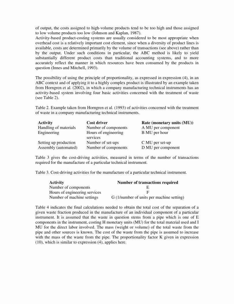
of output, the costs assigned to high-volume products tend to be too high and those assigned to low volume products too low (Johnson and Kaplan, 1987). Activity-based product-costing systems are usually considered to be most appropriate when overhead cost is a relatively important cost element, since when a diversity of product lines is available, costs are determined primarily by the volume of transactions (see above) rather than by the output. Under such conditions in particular, the ABC method is likely to yield substantially different product costs than traditional accounting systems, and to more accurately reflect the manner in which resources have been consumed by the products in question (Innes and Mitchell, 1993). The possibility of using the principle of proportionality, as expressed in expression (4), in an ABC context and of applying it to a highly complex product is illustrated by an example taken from Horngren et al. (2002), in which a company manufacturing technical instruments has an activity-based system involving four basic activities concerned with the treatment of waste (see Table 2). Table 2. Example taken from Horngren et al. (1993) of activities concerned with the treatment of waste in a company manufacturing technical instruments.

Activity Cost driver Rate (monetary units (MU)) Handling of materials Number of components A MU per component Engineering Hours of engineering

services B MU per hour

Setting up production Number of set-ups C MU per set-up Assembly (automated) Number of components D MU per component

Table 3 gives the cost-driving activities, measured in terms of the number of transactions required for the manufacture of a particular technical instrument. Table 3. Cost-driving activities for the manufacture of a particular technical instrument.

Activity Number of transactions required Number of components E Hours of engineering services F Number of machine settings G (1/number of units per machine setting)

Table 4 indicates the final calculations needed to obtain the total cost of the separation of a given waste fraction produced in the manufacture of an individual component of a particular instrument. It is assumed that the waste in question stems from a pipe which is one of E components in the instrument, costing H monetary units (MU) for the total material used and I MU for the direct labor involved. The mass (weight or volume) of the total waste from the pipe and other sources is known. The cost of the waste from the pipe is assumed to increase with the mass of the waste from the pipe. The proportionality factor K given in expression (10), which is similar to expression (4), applies here.

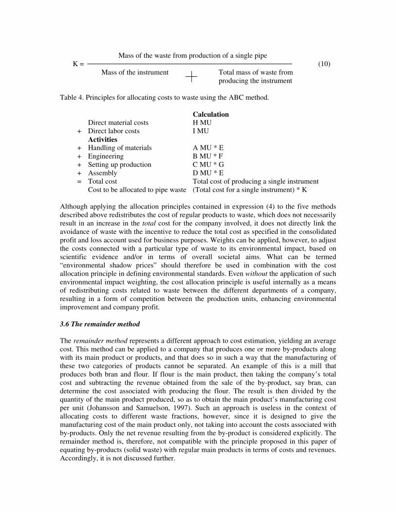
Mass of the waste from production of a single pipe

K = (10) Mass of the instrument Total mass of waste from

producing the instrument

Table 4. Principles for allocating costs to waste using the ABC method.

Calculation Direct material costs H MU + Direct labor costs I MU Activities + Handling of materials A MU * E + Engineering B MU * F + Setting up production C MU * G + Assembly D MU * E = Total cost Total cost of producing a single instrument Cost to be allocated to pipe waste (Total cost for a single instrument) * K

Although applying the allocation principles contained in expression (4) to the five methods described above redistributes the cost of regular products to waste, which does not necessarily result in an increase in the total cost for the company involved, it does not directly link the avoidance of waste with the incentive to reduce the total cost as specified in the consolidated profit and loss account used for business purposes. Weights can be applied, however, to adjust the costs connected with a particular type of waste to its environmental impact, based on scientific evidence and/or in terms of overall societal aims. What can be termed “environmental shadow prices” should therefore be used in combination with the cost allocation principle in defining environmental standards. Even without the application of such environmental impact weighting, the cost allocation principle is useful internally as a means of redistributing costs related to waste between the different departments of a company, resulting in a form of competition between the production units, enhancing environmental improvement and company profit. 3.6 The remainder method The remainder method represents a different approach to cost estimation, yielding an average cost. This method can be applied to a company that produces one or more by-products along with its main product or products, and that does so in such a way that the manufacturing of these two categories of products cannot be separated. An example of this is a mill that produces both bran and flour. If flour is the main product, then taking the company’s total cost and subtracting the revenue obtained from the sale of the by-product, say bran, can determine the cost associated with producing the flour. The result is then divided by the quantity of the main product produced, so as to obtain the main product’s manufacturing cost per unit (Johansson and Samuelson, 1997). Such an approach is useless in the context of allocating costs to different waste fractions, however, since it is designed to give the manufacturing cost of the main product only, not taking into account the costs associated with by-products. Only the net revenue resulting from the by-product is considered explicitly. The remainder method is, therefore, not compatible with the principle proposed in this paper of equating by-products (solid waste) with regular main products in terms of costs and revenues. Accordingly, it is not discussed further.

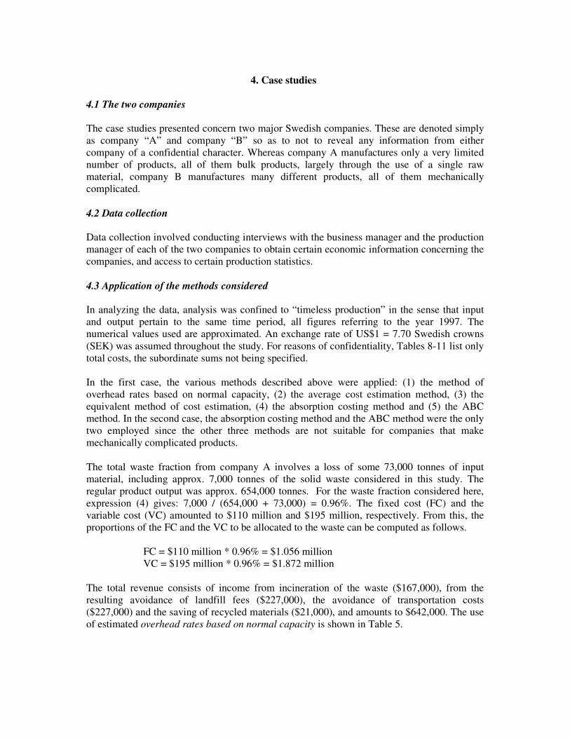
4. Case studies

4.1 The two companies The case studies presented concern two major Swedish companies. These are denoted simply as company “A” and company “B” so as to not to reveal any information from either company of a confidential character. Whereas company A manufactures only a very limited number of products, all of them bulk products, largely through the use of a single raw material, company B manufactures many different products, all of them mechanically complicated. 4.2 Data collection Data collection involved conducting interviews with the business manager and the production manager of each of the two companies to obtain certain economic information concerning the companies, and access to certain production statistics. 4.3 Application of the methods considered In analyzing the data, analysis was confined to “timeless production” in the sense that input and output pertain to the same time period, all figures referring to the year 1997. The numerical values used are approximated. An exchange rate of US$1 = 7.70 Swedish crowns (SEK) was assumed throughout the study. For reasons of confidentiality, Tables 8-11 list only total costs, the subordinate sums not being specified. In the first case, the various methods described above were applied: (1) the method of overhead rates based on normal capacity, (2) the average cost estimation method, (3) the equivalent method of cost estimation, (4) the absorption costing method and (5) the ABC method. In the second case, the absorption costing method and the ABC method were the only two employed since the other three methods are not suitable for companies that make mechanically complicated products. The total waste fraction from company A involves a loss of some 73,000 tonnes of input material, including approx. 7,000 tonnes of the solid waste considered in this study. The regular product output was approx. 654,000 tonnes. For the waste fraction considered here, expression (4) gives: 7,000 / (654,000 + 73,000) = 0.96%. The fixed cost (FC) and the variable cost (VC) amounted to $110 million and $195 million, respectively. From this, the proportions of the FC and the VC to be allocated to the waste can be computed as follows.

FC = $110 million * 0.96% = $1.056 million VC = $195 million * 0.96% = $1.872 million

The total revenue consists of income from incineration of the waste ($167,000), from the resulting avoidance of landfill fees ($227,000), the avoidance of transportation costs ($227,000) and the saving of recycled materials ($21,000), and amounts to $642,000. The use of estimated overhead rates based on normal capacity is shown in Table 5.

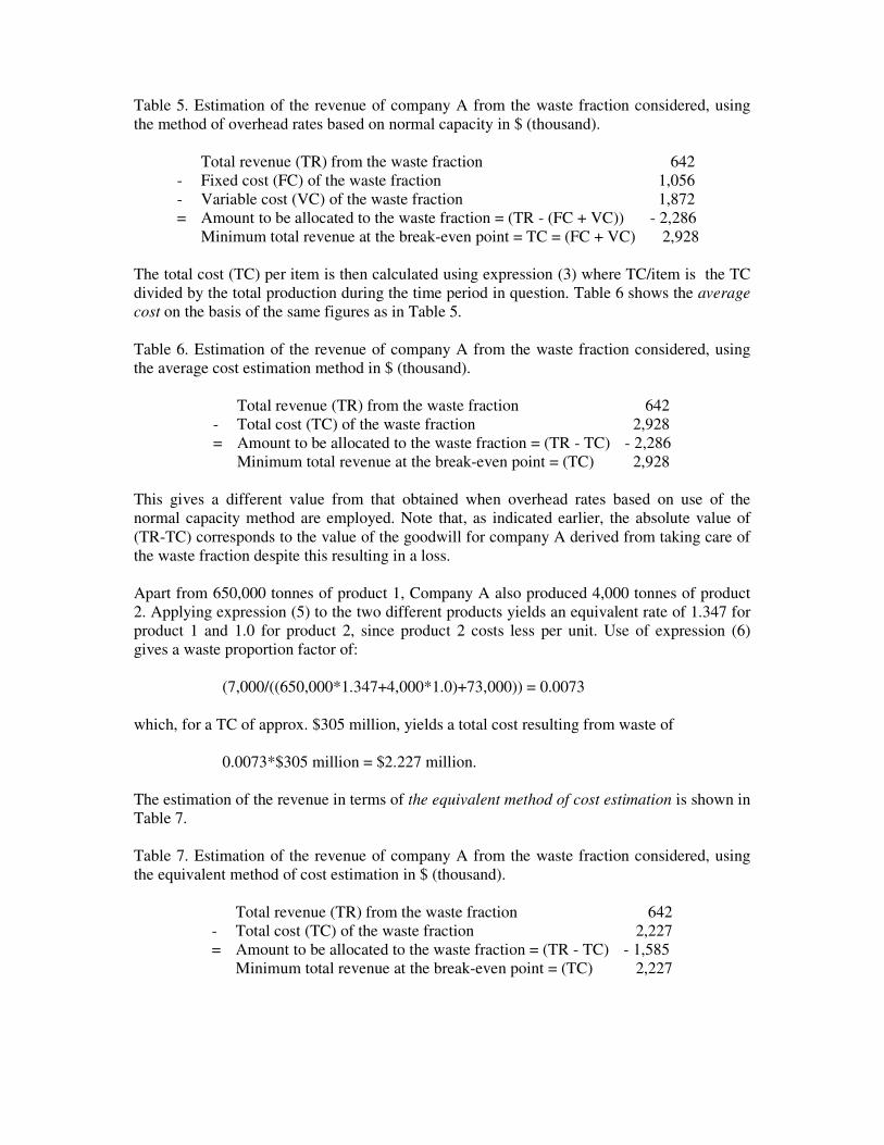
Table 5. Estimation of the revenue of company A from the waste fraction considered, using the method of overhead rates based on normal capacity in $ (thousand).

Total revenue (TR) from the waste fraction 642 - Fixed cost (FC) of the waste fraction 1,056 - Variable cost (VC) of the waste fraction 1,872 = Amount to be allocated to the waste fraction = (TR - (FC + VC)) - 2,286 Minimum total revenue at the break-even point = TC = (FC + VC) 2,928

The total cost (TC) per item is then calculated using expression (3) where TC/item is the TC divided by the total production during the time period in question. Table 6 shows the average cost on the basis of the same figures as in Table 5. Table 6. Estimation of the revenue of company A from the waste fraction considered, using the average cost estimation method in $ (thousand).

Total revenue (TR) from the waste fraction 642 - Total cost (TC) of the waste fraction 2,928 = Amount to be allocated to the waste fraction = (TR - TC) - 2,286 Minimum total revenue at the break-even point = (TC) 2,928

This gives a different value from that obtained when overhead rates based on use of the normal capacity method are employed. Note that, as indicated earlier, the absolute value of (TR-TC) corresponds to the value of the goodwill for company A derived from taking care of the waste fraction despite this resulting in a loss. Apart from 650,000 tonnes of product 1, Company A also produced 4,000 tonnes of product 2. Applying expression (5) to the two different products yields an equivalent rate of 1.347 for product 1 and 1.0 for product 2, since product 2 costs less per unit. Use of expression (6) gives a waste proportion factor of:

(7,000/((650,000*1.347+4,000*1.0)+73,000)) = 0.0073 which, for a TC of approx. $305 million, yields a total cost resulting from waste of

0.0073*$305 million = $2.227 million. The estimation of the revenue in terms of the equivalent method of cost estimation is shown in Table 7.

Table 7. Estimation of the revenue of company A from the waste fraction considered, using the equivalent method of cost estimation in $ (thousand).

Total revenue (TR) from the waste fraction 642 - Total cost (TC) of the waste fraction 2,227 = Amount to be allocated to the waste fraction = (TR - TC) - 1,585 Minimum total revenue at the break-even point = (TC) 2,227

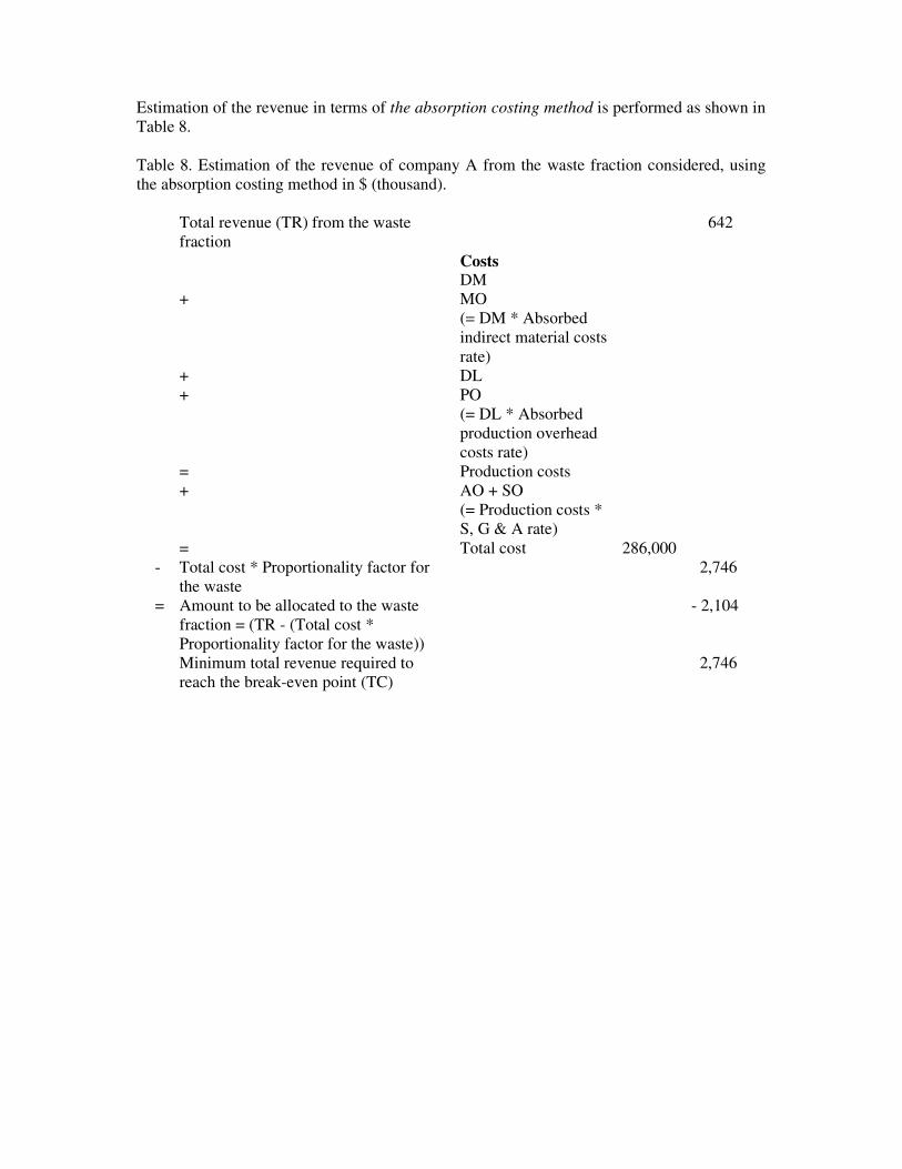
Estimation of the revenue in terms of the absorption costing method is performed as shown in Table 8. Table 8. Estimation of the revenue of company A from the waste fraction considered, using the absorption costing method in $ (thousand).

Total revenue (TR) from the waste fraction

642

Costs DM + MO

(= DM * Absorbed indirect material costs rate)

+ DL + PO

(= DL * Absorbed production overhead costs rate)

= Production costs + AO + SO

(= Production costs * S, G & A rate)

= Total cost 286,000 - Total cost * Proportionality factor for

the waste 2,746

= Amount to be allocated to the waste fraction = (TR - (Total cost * Proportionality factor for the waste))

- 2,104

Minimum total revenue required to reach the break-even point (TC)

2,746

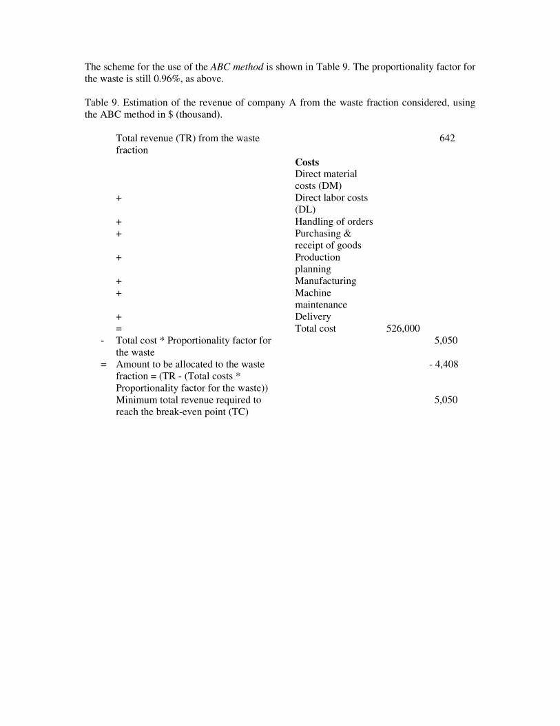
The scheme for the use of the ABC method is shown in Table 9. The proportionality factor for the waste is still 0.96%, as above. Table 9. Estimation of the revenue of company A from the waste fraction considered, using the ABC method in $ (thousand).

Total revenue (TR) from the waste fraction

642

Costs Direct material

costs (DM)

+ Direct labor costs (DL)

+ Handling of orders + Purchasing &

receipt of goods

+ Production planning

+ Manufacturing + Machine

maintenance

+ Delivery = Total cost 526,000 - Total cost * Proportionality factor for

the waste 5,050

= Amount to be allocated to the waste fraction = (TR - (Total costs * Proportionality factor for the waste))

- 4,408

Minimum total revenue required to reach the break-even point (TC)

5,050

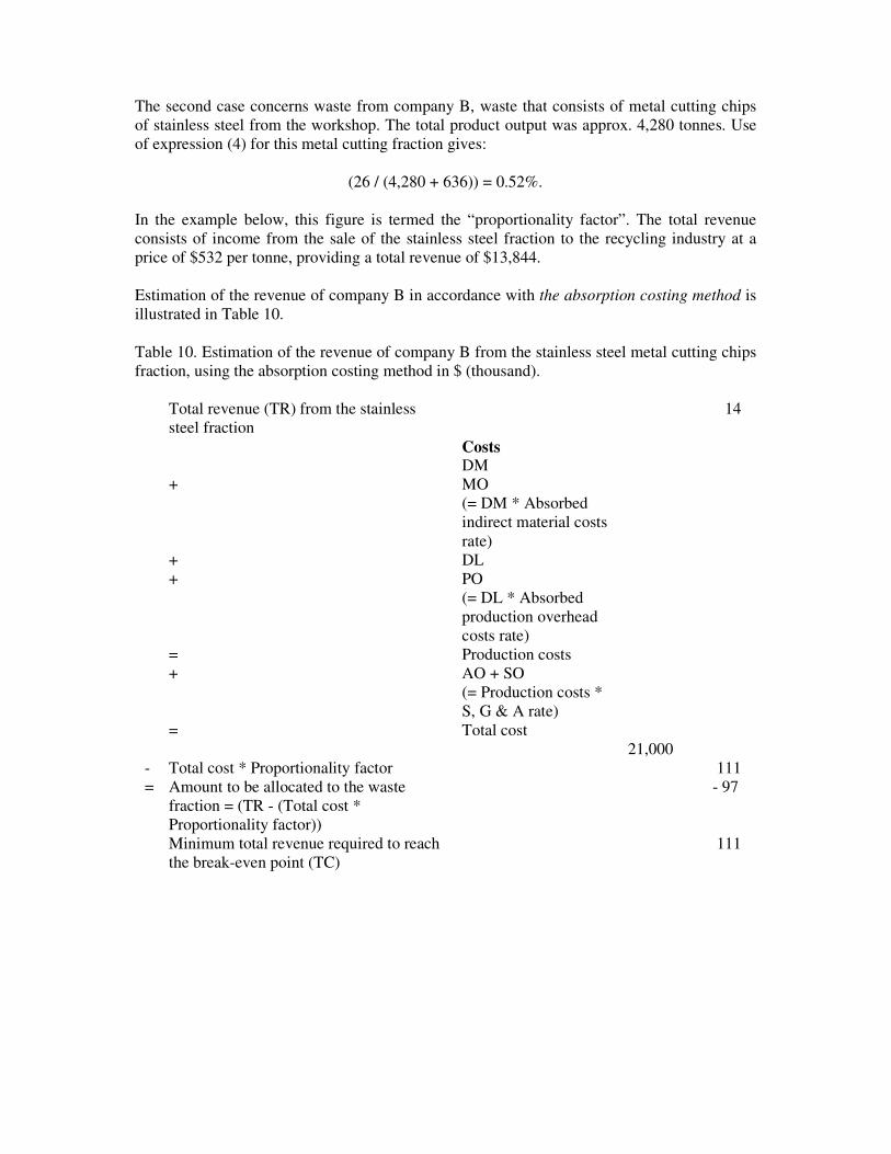
The second case concerns waste from company B, waste that consists of metal cutting chips of stainless steel from the workshop. The total product output was approx. 4,280 tonnes. Use of expression (4) for this metal cutting fraction gives:

(26 / (4,280 + 636)) = 0.52%. In the example below, this figure is termed the “proportionality factor”. The total revenue consists of income from the sale of the stainless steel fraction to the recycling industry at a price of $532 per tonne, providing a total revenue of $13,844. Estimation of the revenue of company B in accordance with the absorption costing method is illustrated in Table 10. Table 10. Estimation of the revenue of company B from the stainless steel metal cutting chips fraction, using the absorption costing method in $ (thousand).

Total revenue (TR) from the stainless steel fraction

14

Costs DM + MO

(= DM * Absorbed indirect material costs rate)

+ DL + PO

(= DL * Absorbed production overhead costs rate)

= Production costs + AO + SO

(= Production costs * S, G & A rate)

= Total cost 21,000

- Total cost * Proportionality factor 111 = Amount to be allocated to the waste

fraction = (TR - (Total cost * Proportionality factor))

- 97

Minimum total revenue required to reach the break-even point (TC)

111

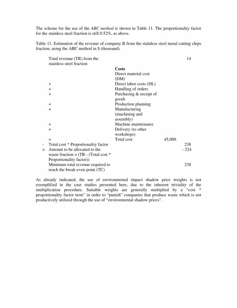
The scheme for the use of the ABC method is shown in Table 11. The proportionality factor for the stainless steel fraction is still 0.52%, as above. Table 11. Estimation of the revenue of company B from the stainless steel metal cutting chips fraction, using the ABC method in $ (thousand).

Total revenue (TR) from the stainless steel fraction

14

Costs Direct material cost

(DM)

+ Direct labor costs (DL) + Handling of orders + Purchasing & receipt of

goods

+ Production planning + Manufacturing

(machining and assembly)

+ Machine maintenance + Delivery (to other

workshops)

= Total cost 45,000 - Total cost * Proportionality factor 238 = Amount to be allocated to the

waste fraction = (TR - (Total cost * Proportionality factor))

- 224

Minimum total revenue required to reach the break-even point (TC)

238

As already indicated, the use of environmental impact shadow price weights is not exemplified in the case studies presented here, due to the inherent triviality of the multiplication procedure. Suitable weights are generally multiplied by a “cost * proportionality factor term” in order to “punish” companies that produce waste which is not productively utilized through the use of “environmental shadow prices”.

5. Discussion and conclusions

The present paper shows how the principle of equating industrial waste with regular products in a business sense can be applied to traditional cost-benefit methods as a financial basis for environmentally friendly waste management. Results of the case studies show that, in terms of the principle of the “true” internal shadow price, the cost of (solid) waste is substantial, the exact costs obtained differing according to the method employed. These differences are not unexpected and are not of major importance here, since the major aim of considering these methods was to investigate the possibility of adapting these methods in a practical context. The applicability of such methods is indeed indicated by the small variations in the estimated total cost of the waste fraction in both companies calculated without employing environmental impact weighting. There appear to be no specific obstacles to applying the proposed equality principle to either a bulk industry or the manufacture of technically complicated products. The methodology suggested can be assumed, therefore, to be generally applicable to all manufacturing companies producing waste. It may be argued that there is a somewhat distorted transfer of costs from the “goods” to the “bads”. No known estimation method, however, yields results that are completely valid. Whenever a direct link is created between losses and the existence of (solid) waste, through cost redistribution and weighting of environmental impact, economic pressure is exerted on industry to introduce environmentally friendly measures that are as effective as possible in reducing waste at the source, measures that also tend to enhance production efficiency. This, in turn, should reduce both the production of waste and the degree of distortion that occurs in cost allocation; distortion that becomes progressively less, due to an increased co-ordination as regards accounting principles, as the geographical area in which the suggested approach is employed is enlarged. There is thus a trade-off between economic exactness and environmental benefits. The main purpose of applying the equality principle is not to maximize company profits, but rather to conserve the environment. However, experience shows that, in the long run, environmental conservation and maximization of profits tend to be consistent with one another. If the equality principle proves to be successful in reducing industrial solid waste and encouraging the better utilization of that which is produced, the principle could undoubtedly be applied to liquid and gaseous waste. Hopefully, the present study will contribute to the acceptance of a new way of regarding waste in a business context and encourage the development of alternatives to traditional taxation practices with the aim of increasing incentives to reduce industrial waste and changing attitudes towards it. Similarly, it is hoped that this study will help bring about a change in the perceived status of industrial waste through emphasizing the financial impact of shadow prices on costs and revenues. Both official recommendations and voluntary environmental agreements concerning the assessment of industrial waste are required so that company budgets and the consolidated profit and loss accounts used externally are affected in a way that “punishes” the excessive production of waste and the failure to utilize it efficiently. Such developments may be necessary to force industry to act in a manner truly in accordance with the ideal of improving the sustainability and productivity of resource use.

Acknowledgements The author would like to thank Professor William Hogland, Department of Technology, University of Kalmar, Sweden, for his useful comments. The author is also grateful to the University of Kalmar, The Kalmar Research and Development Foundation – Graninge Foundation [Kalmar kommuns forsknings- och utvecklingsstiftelse – Graningestiftelsen], the Knowledge Foundation [KK-stiftelsen], the Swedish Association of Graduate Engineers [Sveriges Civilingenjörsförbund (CF)], the ÅF Group [AB Ångpanneföreningen (ÅF)], the Swedish Research Council for Environment, Agricultural Sciences and Spatial Planning [Forskningsrådet för miljö, areella näringar och samhällsbyggande (FORMAS)] and the Development Fund of the Swedish Construction Industry [Svenska Byggbranschens Utvecklingsfond (SBUF)] for financial support.

References Asplund, E. et al., 1994. Byggandet i kretsloppet: miljöeffekter, kostnader och konsekvenser.

Stockholms byggförlag, Stockholm, Sweden. Barlishen, K.D., Baetz, B.W., 1996. Development of a Decision Support System for Municipal

Solid Waste Management Systems Planning. Waste Manage. & Res. 14: 71-86. Bromwich, M., Bhimani, A., 1989. Management Accounting: Evolution not revolution.

CIMA, London, UK. Freeman, H. (Ed.), 1995. Industrial Pollution Prevention Handbook. McGraw-Hill, New York,

U.S.A. Gerdin, J., 1995. ABC-kalkylering. Studentlitteratur, Lund, Sweden. Horngren, C.T.; Sunden, G.L. and Selto, F.H., 2002. Introduction to Management Accounting.

Prentice-Hall International, London, UK. Innes, J., Mitchell, F., 1993. Overhead Cost. Academic Press, London, UK. Jasch, C. Environmental Performance Evaluation. The Links between Financial and

Environmental Management. Challenges and Approaches to Incorporating the Environment into Business Decisions. Invitational Expert Seminar, 3-5 June 1996, Opio, France.

Johansson, S.-E., Samuelson, L.A., 1997. Industriell kalkylering och redovisning. Norstedts

Juridik, Stockholm, Sweden. Johnson, H.T., Kaplan, R.S., 1987. Relevance Lost. The Rise and Fall of Management

Accounting. Harvard Business School Press, Boston, U.S.A. Kretsloppsdelegationen 1997. Producentansvar för varor. Förslag och idé, Report 1997:19.

Stockholm, Sweden. Olsson, J., Skärvad, P.-H., 2000. Företagsekonomi 99. Liber-Hermods, Malmö, Sweden. Svensk Författningssamling (SFS) 1999:673, 1999. Lag om skatt på avfall. Stockholm,

Sweden. UNCED, 1992. Report of the United Nations Conference on Environment and Development,

Chap. 30.