Environmental investment decisions: experimental evidence

ISSN 1403-2473 (Print) ISSN 1403-2465 (Online)

Working Paper in Economics No. 719

Environmental investment decisions: experimental evidence of team versus individual decision making Simon Felgendreher, Magnus Hennlock, Åsa Löfgren, Conny Wollbrant Department of Economics, January 2018

1

Environmental investment decisions: experimental

evidence of team versus individual decision making

Simon Felgendreher, Magnus Hennlock, Åsa Löfgren, Conny Wollbrant*

Abstract

We study experimentally how investment decisions are affected by equally stringent but

different policy regime treatments and how differences depend on whether decisions are made

individually or in groups. In our experiment, subjects decide on an investment level either

individually or jointly in groups of three. In addition, decisions are made subject to either a

tax or performance standard treatment. We find that investments are significantly higher and

closer to the level that maximizes revenues of the hypothetical firm in the performance

standard treatment. This holds for both individual and group decisions, but we find no

evidence of an interaction effect. Even though groups seem to have a knowledge advantage,

they are not able to benefit from it, since intragroup communication is not able to transmit the

microeconomic reasoning to group members without such knowledge. Also, groups are not

able to attenuate the attention bias of focusing on selective information depending on the

specific policy treatment.

Key Words: group behavior, investment inefficiencies, policy instruments

JEL Classification: C92, D70, H32

* Felgendreher, Department of Economics, University of Gothenburg, P.O. Box 640, S-405 30 Gothenburg, Sweden, tel: +46 31 786 2552, e-mail: [email protected]. Hennlock, Policy and Economy, IVL Swedish Environmental Research Institute, P.O. Box 530, 21 S-400 14 Gothenburg, Sweden, tel: +46 31 708 65 08, e-mail: [email protected]. Löfgren, Department of Economics, University of Gothenburg, P.O. Box 640, S-405 30 Gothenburg, Sweden, tel: +46 31 786 1375, e-mail: [email protected]. Wollbrant, Department of Economics, University of Stirling, FK94LA Stirling, United Kingdom, e-mail: [email protected]. The authors gratefully acknowledge financial support from the Mistra INDIGO research program (the Swedish Foundation for Strategic Environmental Research).

2

1. Introduction

Individuals are often confronted with complex information when they have to make

optimization decisions. In sectors where the price structure is usually nonlinear, such as the

electricity or water sector, it has been found that consumers base their consumption decision

mainly on the average price rather than the marginal price (Shin 1985; Binet et al. 2014; Ito

2014). Also, when it comes to allocating time between taxed and tax-exempt activities, many

individual focus on the average tax rate (de Bartolome 1995). Not only is this behavior

observed among consumers making decisions, but it is also found that firms deviate from

profit maximization in many situations (Armstrong and Huck 2010). One explanation for such

deviations is that managers have access to limited information or the information is too

complex, making it difficult to examine all investment alternatives and identify the optimum.

Instead, managers might apply simplified choice rules, relying on rules of thumb. One such

choice rule is to choose the first investment alternative that is considered satisfactory rather

than compare all investment alternatives. Simon (1955) and Cyert and March (1963) refer to

such a choice rule under bounded rationality as “satisficing.”

In a recent artefactual experiment, Hennlock et al. (2017) tested how high-level

industry managers and senior advisors made an investment decision under different

environmental policy regimes. The authors found that managers in many cases applied choice

rules that conflict with standard economic theory. Similar to the findings by Shin (1985),

Binet et al. (2014), and Ito (2014), the prevalent choices decision-makers made in the

experiment were consistent with minimizing the average cost of abatement in the treatments

based on price instruments (tax and subsidy treatment). In a performance standard treatment,

however, the choices were, on average, closer to the optimizing behavior prescribed by

standard economic theory.

The question that we address in this paper is whether joint decision-making by a group

of individuals can enhance investment decisions like the one presented in Hennlock et al.

(2017). More specifically, we are interested in analyzing whether groups are better than

individuals at taking into account the importance of marginal costs and, as a consequence, are

more likely to apply choice rules that are in line with standard economic theory when

information is limited.

Group decision-making is a common arrangement for overcoming informational

limitations and may ameliorate any effects of bounded rationality observed at the level of the

individual decision-maker (e.g., Fahr and Irlenbusch 2011). The literature on group decision-

3

making in economics suggests that decisions can be considerably improved when made by a

group rather than individually (for an overview, see Charness and Sutter 2012). In contrast,

the literature in psychology on individual versus group decision-making focuses more on the

properties of the decision task to explain when individuals may or may not perform better

than groups. The main distinction is made between intellective and judgmental tasks

(Laughlin and Ellis 1986; see section 2.4 for further discussion). An intellective task has an

objectively correct solution, whereas a judgmental task does not. Moreover, for intellective

tasks, the degree of demonstrability is an important characteristic. If an individual is able to

demonstrate to others the superiority of one possible solution over the alternatives, it has been

shown that groups perform better than individuals at making such decisions (e.g., Laughlin et

al. 2002; Maciejovsky and Budescu 2007).

In this paper, we explore group versus individual decision-making in a setting where

decisions can arguably be characterized as intellective tasks, but where there are limits to the

demonstrability. This setting is relevant especially in situations where decisions need to be

made based on limited information, which is true in many real-world situations. To test

whether choice rules differ between individuals and groups, we extend the design of

Hennlock et al. (2017). We use two of their treatments, the tax and performance standard

treatments, and analyze in a between-subject design whether investment decisions made by

groups of three differ from those of individual decision-makers.

Our experiment was conducted with undergraduate students at the School of Business,

Economics and Law at the University of Gothenburg. In the first part of the experiment,

students solved a task asking them to maximize revenue of a firm by choosing an investment

level, either individually or in groups of three. As a basis for the investment decision, a set of

information parameters (on marginal cost, average cost, and performance level) was provided

in the decision task. In the second part, all students provided individual answers to a survey.

We find significant differences in investment decisions between the tax and

performance treatments. Subjects invested significantly more in the performance treatment

than in the tax treatment. This is partly explained by differences in subjects’ stated level of

attention to information variables in the decision task. In the tax treatment, subjects reported

paying more attention to cost-related variables, while in the performance standard treatment,

subjects relied more on information about the performance of the investment level. These

results therefore replicate the findings of Hennlock et al. (2017). Furthermore, the

performance of groups did not differ significantly from that of individuals, either in the

performance standard or in the tax treatment. Even though we find that knowledge about

4

microeconomic foundations significantly increases the probability of applying the choice rule

prescribed by standard economic theory, the groups were not able to benefit more than

individuals from this knowledge advantage. This suggests that communicating the economic

reasoning within groups in which at least one group member has knowledge about the choice

rule as prescribed by standard economic theory fails to improve decision-making. Also, we

find no evidence that groups are able to attenuate the attention bias of focusing on selective

information based on the policy instrument.

The paper is organized as follows. The experimental design and procedures are

described in section 2. The results are presented in section 3. Section 4 concludes.

2. Survey Design and Experimental Manipulations

2.1. Population, participants, and execution of the experiment

The experiment was conducted January 18–21, 2016, at the School of Business, Economics

and Law at the University of Gothenburg, Sweden. This was the first week of the spring

semester, and the dates were carefully chosen to both facilitate the execution of the

experiment and maximize the number of participants. The director of studies and student

administrators provide general information to all classes in economics and statistics during the

first lecture each semester, and we enlisted the director of studies to invite the students to

participate in the experiment.

The invitation to participate in the experiment was framed as follows: At the end of the

information session, the director of studies told the students about the possibility of being part

of a panel that voluntary participates in experiments conducted by economics and finance

researchers at the school. Further, the students would have an opportunity to participate in a

classic pen-and-paper experiment that would end the information session. The students were

informed that participants could earn between 40 and 100 Swedish kronor (approximately

US$4.70–11.70), depending on performance. On average, students earned 82 Swedish kronor

(about US$9.50). The payment was made via the Swedish finance technology app Swish,

transferring the money between bank accounts using only the students’ cell phone numbers,

or alternatively over the counter a few days later at the student administration office.

Approximately 90 percent of students chose to have the payment transferred to them using

Swish.

5

While participation was voluntary, all students were asked to stay in their seats throughout the

pen-and-paper experiment even if they chose not to participate. Altogether, students enrolled

in five different undergraduate courses were invited to participate in the experiment

conducted at the end of the first lecture hour of each class: one class in basic economics, one

class taking economics courses as electives, one class in intermediate economics, one class

attending a specialization course in economics (econometrics at the bachelor’s level), and one

basic statistics class. By choosing economics students for the experiment, we wanted to

guarantee that a share of students had taken basic microeconomic courses and were familiar

with solving optimization tasks. The registered number of students in these courses was 862,

but fewer students attended the lectures.1 In total, 578 students participated in the experiment.

Eight observations were dropped, leaving a total of 570 observations.2

The experiment was divided into two parts. In the first part, working either individually or in

teams of three, participants solved the decision task to maximize the net return of a

hypothetical firm by choosing an investment level subject to either a tax or performance

standard treatment (explained in detail in sections 2.2 and 2.3). In the second part, all

participants answered a survey individually. The experiment lasted for 30 to 40 minutes, and

all participants were monitored by the researchers and four to six research assistants (the

number of assistants varied depending on class size). See section A.2.2 in the appendix for the

full survey.

2.2. Treatments

After the invitation to participate in the experiment, the research assistants handed out

envelopes. Students who chose to participate either shared an envelope in a group of three or

received an envelope individually. In the envelopes that were distributed was an instruction

page and additional envelopes for part one and two of the experiment. All students were

instructed to leave the envelopes closed until further notice. After each participating student

or group had received an envelope, the director of studies told the students to open the

1 The main reason for not attending the information session was that it was not mandatory. Especially for students who were enrolled in a course to retake an exam, the information session did not provide much new information. 2 The observations were dropped because the student did not answer the main question (1 observation), students were talking to their neighbors (4 observations), or one of the group members left the room (3 observations).

6

envelope and take out the instruction page (in yellow for ease of reference). The instructions

were read out loud to the class (see section A.2.1 in the appendix for details).

Then the participants took out the envelope for part one of the experiment (in white) and

started to solve the task: to choose which of six investment alternatives would yield the

highest net revenue for a hypothetical firm (further described in section 2.3). The students

were asked to talk quietly within the groups (figure A.1 in the appendix is a photo from one of

the sessions). We did not observe any communication between groups or individuals during

the sessions (other than in the dropped observations noted above), and the same protocol was

followed strictly for each session. Of the 570 students who completed the experiment, 414

were assigned to groups (yielding 138 group responses) and 156 to the individual treatments.

The two treatments differed only in the instructions about the regulatory information shown in

table 1. This design ensures that the stringency of the two policy instruments is identical.

Table 1. Policy instrument treatments

Treatment Regulator’s information

Performance standard The condition for your investment decision is that the firm should meet an

emissions limit of 75 grams per kWh output on an annual average basis

according to the Swedish Environmental Code.

Tax The condition for your investment decision is that the firm will pay an

emissions tax of SEK 250 per kg of emissions each year.

Note: kWh = kilowatt hours; SEK = Swedish crowns; kg = kilograms

The assignment of groups and individuals to the two treatments was done in a semirandom

way by successively assigning the four possible conditions.3 To form groups of three, students

sitting next to each other were asked to work together during the experiment. The main reason

for not assigning treatment randomly and reshuffling students to groups was that changing the

seating in the lecture halls would have been too time-consuming and probably would have led

to a high dropout rate. Because groups were not assigned randomly and might differ with

respect to how well group members knew each other beforehand, we asked for this

information explicitly in the ex post survey.

Of the 570 students who completed the experiment, 283 were assigned to the tax treatment

and 287 to the performance standard treatment. Table 2 reports the number of groups and

individual subjects (by course/session and decision treatment, tax versus performance 3 Treatment tax and individual; treatment tax and group; treatment performance standard and individual; treatment performance standard and group.

7

standard). Two-sided tests of pairwise comparison of all possible combinations of the four

treatments does not yield significant differences in the characteristics and study programs at a

5 percent significance level.

Table 2. Descriptive statistics

Variable Description All students (n = 570)

Tax treatment: individual (n = 76)

Tax treatment:

group (n = 207)

Performance standard: individual (n = 80)

Performance standard: group

(n = 207)

Background characteristics (shares)

Female =1 if the student is female

0.45 0.37 0.48 0.39 0.48

Age Age in years (min 19, max 71)

23.7 23.9 23.7 24.3 23.3

Microeconomics

=1 if course taken

0.37 0.37 0.39 0.39 0.35

Study program (number of students) Basic economics

188 22 72 25 69

Elective courses in economics

141 21 45 21 54

Intermediate economics

100 12 39 13 36

Specialization courses in economics

64 12 21 10 21

Basic statistics 77 9 30 11 27 Note: Two-sided t-tests of pairwise comparison of all four treatments do not yield significant differences in the background characteristics and in the study program chosen, at a significance level of 5%.

2.3. The decision task and incentives

As in Hennlock et al. (2017), the decision task to maximize the net return of a firm was

presented to the students as a choice among six different investment alternatives. For each

investment alternative, three different categories of information were provided:

1. regulatory information about the stringency and type of policy instrument in place

(varies across treatments; see table 1, tax versus performance standard);

2. emissions performance levels in grams of emissions per kilowatt hours (g/kWh) of

output for each of the six investment alternatives (identical across treatments); and

8

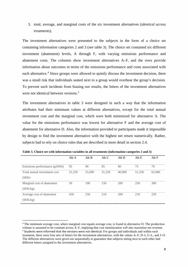
3. total, average, and marginal costs of the six investment alternatives (identical across

treatments).

The investment alternatives were presented to the subjects in the form of a choice set

containing information categories 2 and 3 (see table 3). The choice set contained six different

investment (abatement) levels, A through F, with varying emissions performance and

abatement costs. The columns show investment alternatives A–F, and the rows provide

information about outcomes in terms of the emissions performance and costs associated with

each alternative.4 Since groups were allowed to quietly discuss the investment decision, there

was a small risk that individuals seated next to a group would overhear the group’s decision.

To prevent such incidents from biasing our results, the letters of the investment alternatives

were not identical between versions.5

The investment alternatives in table 3 were designed in such a way that the information

attributes had their minimum values at different alternatives, except for the total annual

investment cost and the marginal cost, which were both minimized for alternative A. The

value for the emissions performance was lowest for alternative F and the average cost of

abatement for alternative D. Also, the information provided to participants made it impossible

by design to find the investment alternative with the highest net return numerically. Rather,

subjects had to rely on choice rules that are described in more detail in section 2.4.

Table 3. Choice set with information variables in all treatments (information categories 2 and 3)

Alt A Alt B Alt C Alt D Alt E Alt F

Emissions performance (g/kWh) 95 90 85 80 75 70

Total annual investment cost

(SEK)

21,250 25,000 31,250 40,000 51,250 65,000

Marginal cost of abatement

(SEK/kg)

50 100 150 200 250 300

Average cost of abatement

(SEK/kg)

430 250 210 200 210 220

4 The minimum average cost, where marginal cost equals average cost, is found in alternative D. The production volume is assumed to be constant across A–F, implying that cost minimization will also maximize net revenue. 5 Students were informed that the versions were not identical. For groups and individuals and within each treatment, there were four sets of letters for the investment alternatives, with the values A–F, D–I, G–L, and J–O. The different alternatives were given out sequentially to guarantee that subjects sitting next to each other had different letters assigned to the investment alternatives.

9

The underlying cost function for table 3, which was not known to the experiment participants,

is given by the following equation:

𝑇𝑇𝑇𝑇𝑇𝑇𝑇𝑇𝑇𝑇 𝑐𝑐𝑇𝑇𝑐𝑐𝑇𝑇(𝑇𝑇𝑎𝑎𝑇𝑇𝑇𝑇𝑎𝑎𝑎𝑎𝑎𝑎𝑎𝑎𝑇𝑇) = 20,000𝑆𝑆𝑆𝑆𝑆𝑆 + (𝑇𝑇𝑎𝑎𝑇𝑇𝑇𝑇𝑎𝑎𝑎𝑎𝑎𝑎𝑎𝑎𝑇𝑇2)𝑆𝑆𝑆𝑆𝑆𝑆/2.

Without any abatement, 1,000 units of emissions are assumed to be produced. Investment

alternative A abates 50 units and emissions are 950. The investment alternatives increase the

abatement level by 50 consecutively, so that at alternative F, abatement is 300 and emissions

are 700. Figure 1 graphically illustrates the underlying continuous cost function with each

investment alternative depicted in the graph. Alternative A has the lowest investment cost, but

under the performance standard, alternative E has the lowest cost that complies with the

emissions limit. For the environmental tax, not only the annual investment cost has to be

considered, but also the tax that has to be paid for each unit of emissions that is not abated.

Figure 2 depicts the sum of these costs for each investment alternatives, and as can be seen,

alternative E has the lowest total cost when the environmental tax is applied. Thus, the

optimal investment choice is the same in the performance standard and the tax treatment.

Figure 1. Total annual investment cost for each investment alternative (not shown in the experiment)

0

10 000

20 000

30 000

40 000

50 000

60 000

70 000

Alt. A Alt. B Alt. C Alt. D Alt. E Alt. F

Tota

l ann

ual i

nves

tmen

t cos

t (in

SEK

)

10

Figure 2. Total cost for each investment alternative in the tax treatment (not shown in the experiment)

Immediately after making the investment choice, subjects were asked to grade, on a six-item

Likert scale, how relevant each information attribute was for their choice.

The participants were informed that their payoff would be determined by their performance—

that is, the higher the corresponding net return from the investment (as given by the

underlying cost function), the higher the payoff to the individual or group. The investment

alternatives gave the following payoffs: alternative E yielded a payoff of 100 SEK, D or F

yielded 80 SEK, C yielded 70 SEK, B yielded 60 SEK, and A yielded 40 SEK. For those in a

group, each member received the full payoff for the alternative the group chose.

2.4. Definition of the task

Economic experiments of group decision-making have mainly focused on error rates when

evaluating probabilities.6 Researchers have studied variations of the conjunction fallacy

experiment, first introduced by Tversky and Kahneman (1983). The setting in these tasks is

chosen in such a way that the correct solution can be easily calculated by applying logical

reasoning but is in contrast to the intuitive heuristics many people base their decisions on. It is

6 A variety of group experiments in economics have been conducted in interactive settings, such as beauty contest or market entry games (see, for instance, Cooper and Kagel 2005; Kocher and Sutter 2005; Kugler et al. 2012). In this class of experiments, the task is mainly to update beliefs about the behavior of the other players’ actions correctly, so the tasks are quite different from those in our setting and therefore are not discussed here in detail.

225 000

230 000

235 000

240 000

245 000

250 000

255 000

260 000

265 000

Alt. A Alt. B Alt. C Alt. D Alt. E Alt. F

Tota

l anu

ual i

nves

tmen

t cos

t and

tax

paym

ents

(in

SEK)

11

found that groups are systematically better in identifying the correct solution in such cases

(Charness et al. 2007, 2010).

The psychology literature makes a distinction between intellective and judgmental tasks. An

intellective task is defined by having a correct solution, such as a mathematical optimization

problem. In contrast, a judgmental task lacks such a correct answer, and the solution might

depend on individuals’ preferences and beliefs. If a task is intellective, it can be further

defined by the extent to which the correct solution is demonstrable to other group members

(Laughlin 1980). The degree of demonstrability of a task depends on four characteristics:

First, group members must have a common conceptual system (for example, a mathematical

or verbal system). Second, they must have sufficient information to solve the problem. Third,

group members must be able to understand the reasoning of the person knowing the answer.

And fourth, the person knowing the correct answer must be able to explain the correct

solution to the other group members (Laughlin and Ellis 1986). The higher the degree of

demonstrability, the better the performance of groups should be compared with individuals in

solving a task. Given that at least one group member knows the correct solution, it should be

easier to convince the other group members of the solution the higher the demonstrability of

the task. Empirical evidence in psychology has shown that groups have an advantage over

individuals when solving tasks with a high degree of demonstrability (Laughlin et al. 2002;

Maciejovsky and Budescu 2007).

In line with the description above, we characterize the tasks in both the tax and performance

standard treatment as intellective, since in theory each has a correct and unique cost-

minimizing solution. However, based on the information provided in the treatments, this

solution is not numerically verifiable by participants in the experiment. Instead, the task has to

be solved using a simplified choice rule. Based on economic theory, the choice rule that

maximizes the net revenue for the firm in the case of the performance standard is the one that

does not exceed the emissions limit and has the lowest total cost of abatement among the

remaining options. In the tax treatment, the choice rule maximizing the net revenue for the

firm corresponding to standard economic theory is to set the marginal cost of abatement equal

to the emissions tax rate. Given the information provided, it is also possible to apply choice

rules that do not necessarily maximize the net revenue for the firm. An overview of possible

choice rules is given in table 4. Independent of the treatment, subjects might base their

decision on minimizing a specific cost variable, which would lead to different investment

alternatives as summarized under “General choice rules” in table 4. There also exist

12

treatment-specific choice rules, such as choosing the investment alternative where the tax

equals the average cost of abatement in the tax treatment. In the performance standard

treatment, minimizing any of the cost variables conditional on not exceeding the emissions

limit will lead to the same investment alternative choice.

Table 4. Possible choice rules when choosing an investment alternative

Possible choice rules Investment

alternative

General choice rules

Minimize emissions performance F

Minimize total annual investment cost A

Minimize marginal cost of abatement A

Minimize average cost of abatement D

Choice rules in the performance standard treatment

Minimize total annual investment cost/marginal cost of abatement/average cost of

abatement given that the emissions limit is not exceeded

E

Choice rules in the tax treatment

Tax equal to marginal cost of abatement E

Tax equal to average cost of abatement B

The extent to which the choice rules that maximize the net revenue for the firm are

demonstrable to other group members varies broadly between the two treatments. In the

performance standard treatment, the information provided to participants states that the

emissions should not exceed 75 grams per kWh output. Looking at the information variables

given for the investment alternatives, it should be relatively easy to identify that the emissions

performance from investment alternatives A to D exceeds the allowed emissions and therefore

should not be taken into account. This reasoning should also be easy to demonstrate to other

group members, since one just has to point at the row with the emissions performance of the

different investment alternatives. As a second step, groups have to decide between

alternatives E and F. The optimization rule here is to take the investment alternative with the

lowest total annual investment cost (E). If all group members have sufficient knowledge of

microeconomic foundations to understand this reasoning, it should be relatively easy for one

group member to explain which alternative to choose and convince the other group members.

Without the knowledge, the demonstrability of the choice rule is lower, but the alternatives to

choose from should at least be narrowed down to two out of the six investment alternatives (E

and F, which comply with the performance standard), as summarized in table 4.

13

In the tax treatment, the degree of demonstrability of the revenue-maximizing alternative

depends on the knowledge of the optimality condition that the marginal cost of abatement

should be equal to the tax rate in order to minimize costs. If at least one group member has

this knowledge and is able to explain the reasoning to the other group members, the degree of

demonstrability is relatively high. If none of the group members has this knowledge, it is hard

or even impossible to demonstrate the choice rule to other group members.

Hence, we argue that the demonstrability is in general higher in the performance standard than

in the tax treatment. However, this does not necessarily mean that groups are more likely than

individuals to choose the investment level that is in line with the net revenue-maximizing

choice rule under the performance standard. If finding the net revenue-maximizing choice rule

is relatively simple for individuals under the performance standard such that most are able to

identify it, there may not be an advantage for group members to demonstrate this choice rule

to each other. Therefore, we hypothesize that groups will perform at least equally well as

individuals in the performance standard treatment.

In the tax treatment, we expect that the demonstrability within groups is relatively high if (i)

groups have at least one member with knowledge of the optimality condition, (ii) the group

member with the information is able to explain the reasoning to the other members, and (iii)

the other members are able to follow the reasoning of the knowledgeable group member. We

hypothesize that groups will be more successful than individuals in identifying the revenue-

maximizing choice rule (in accordance with standard economic theory) given that conditions

(i)–(iii) are fulfilled in the tax treatment.

3. Results

3.1. Treatment effects

We start by analyzing differences between the tax treatment and the performance standard

treatment. Summary statistics of the investment alternatives chosen are shown in table 5 and

figure 3. Comparing differences in the distribution between the two policy treatments (and

aggregating decisions made by groups and individuals), we find that investment levels are

significantly lower in the tax treatment compared with the performance standard (p < 0.01,

Mann-Whitney test). This result holds when the difference between the tax and the

performance standard is compared within the individual treatments and within the group

14

treatments.7 Furthermore, in the tax treatment, choices appear slightly more evenly distributed

across alternatives compared with the performance treatment, where alternative E is the most

frequent choice. This holds in both the individual and the group treatments.

In the performance standard treatment, the most frequently chosen alternative is E; 59 percent

(individual) and 49 percent (groups) chose this alternative. This alternative has the lowest

total annual investment cost between the two alternatives that comply with the standard. In the

tax treatment, only 11 percent of individuals and 4 percent of groups chose investment

alternative E. The most commonly chosen alternative in the tax treatment was instead

alternative D (44 percent of individuals and 49 percent of groups), consistent with a choice

rule of minimizing average cost in the task. Hence, the results comparing policy treatments

are overall consistent with the results found in Hennlock et al. (2017). Our results are also in

line with the findings of Shin (1985), Binet et al. (2014), and Ito (2014). These studies find

that individuals, when faced with a complex decision situation, tend to base their consumption

decision mainly on average price rather than marginal price.

Table 5. Summary statistics of investment decision: the percentage of subjects choosing the different investment alternatives in each treatment

Choice alternative A B C D E F

Tax

Individual 0.02 0.17 0.21 0.44 0.11 0.04

Group 0.01 0.06 0.38 0.49 0.04 0.01

Performance standard

Individual 0.03 0.01 0.11 0.21 0.59 0.05

Group 0.00 0.09 0.13 0.25 0.49 0.04

Note: The cells highlighted in gray show the modal response in the particular treatment.

Figure 3. Investment choice by treatment

7 p < 0.01 for Mann-Whitney tests in both subsamples.

15

A comparison between individual and group treatments shows that the distribution of

frequencies in the tax treatment seems to be more dispersed in the individual treatment than in

the group treatment, in which alternatives C and D have relatively larger frequencies. A

Mann-Whitney test, however, does not detect any significant difference between the

individual and group treatments (p = 0.7487). In the performance treatment, the differences

are less clear, and again a Mann-Whitney test does not yield any significant difference (p =

0.1940).

To test whether the treatments can provide an explanation for observed investment choices,

we use a multinomial logit model with the investment choice as the dependent variable and

the treatments as independent dummy variables. The marginal effects are discrete changes

compared with the baseline level (individual decisions in the performance standard

treatment). Table 6 contains the predicted probabilities and marginal effects of the

multinomial logit model.

Table 6. Predicted probabilities and average marginal effects on choice in the multinomial logit model Multinomial logit model


Tax -0.000 0.208*** 0.072 0.166** -0.430*** -0.014

(0.018) (0.080) (0.067) (0.083) (0.067) (0.026)

Group -0.251*** 0.152* 0.074 0.085 -0.054 -0.006

(0.011) (0.084) (0.047) (0.069) (0.046) (0.022)

TaxXGroup 0.221** -0.236** 0.112 0.047 -0.123 -0.022

(0.106) (0.094) (0.100) (0.127) (0.128) (0.050)

Predicted average 0.017** 0.078*** 0.204*** 0.350*** 0.313*** 0.037***

Probability (0.008) (0.015) (0.023) (0.027) (0.023) (0.011)

Prob > chi2 0.000

Observations 294 294 294 294 294 294

Note: Robust standard errors in parentheses; * p < 0.1, ** p < 0.05, *** p < 0.01.

The differences in choices between groups and individuals are indicated by the “Group”

dummy variable in the regression. Here, groups are significantly less likely than individuals to

choose alternative A, while they are more likely to choose B. However, there is no difference

between groups and individuals in choosing the cost-minimizing alternative E. Also in the tax

treatment, there is no significant difference in choosing alternative E between groups and

individuals (see coefficients for “TaxXGroup”). In contrast to the performance standard, the

16

choices between alternatives A and B are reversed: groups are significantly more likely than

individuals to choose A, while they are less likely to choose B.

3.1. Investment choice and background knowledge

In the questionnaire following the experiment, we asked all subjects for the optimality

condition for a firm to maximize its net revenue in response to an environmental tax

according to standard economic theory. Out of four possible answers, only one was correct.

The question was number 6 in the survey, so we refer to it as “Q6” in the following

discussion. The exact wording can be found in section A.2.3 in the appendix.

We assume that individuals who answer this question correctly are more likely to choose

alternative E, which is in line with the revenue-maximizing choice rule. Table 7 gives an

overview of how the participants answered Q6. As can be seen in the first two columns, in the

tax treatment, 54 percent of groups had at least one member that answered the question

correctly, whereas only 29 percent of individuals chose the correct answer.8 These numbers

are close to the percentages we would expect if individuals would randomize over alternatives

in Q6. Choosing one of the four alternatives in Q6 at random, we would expect that 58

percent (= 1 – 0.753) of groups have at least one member that chooses the correct answer and

25 percent of individuals answer correctly. However, individuals who have taken the basic

microeconomic course before participating in the experiment were more likely to answer

question 6 correctly (see table A.1 in the appendix). If the answers were completely random,

we would not expect to see a correlation between the two variables.

8 For the performance standard, the answers to Q6 were similar, as shown in the lower part of table 7. Since it is of little importance to know the optimality condition to identify the cost-minimizing investment alternative E under a performance standard, we do not discuss this case further.

17

Table 7. Summary statistics of the correct answer to question 6

Share of answers to

question 6

(number of observations in

parentheses)

Frequency of number of group members

answering question 6 correctly

(number of observations in parentheses)

Total number of

observations

Incorrect Correct* 1 2 3

Tax

Individual 0.71 0.29

(54) (22) (76)

Group 0.46 0.54 0.39 0.10 0.04

(32) (35) (27) (7) (1) (67)

Performance standard

Individual 0.83 0.18

(66) (14) (74)

Group 0.54 0.46 0.36 0.09 0.01

(37) (32) (25) (6) (1) (69)

* Group observations were counted as answering the question correctly if at least one group member answered

the questions correctly.

Further, if answers to Q6 were completely random, we would not expect that it has a

significant influence on choosing the cost-minimizing investment alternative, either. Table 8

shows results for a multinomial logit model where the answer to Q6 is the regressor and the

different investment alternatives serve as dependent variables. The table depicts estimates for

average marginal effects, and predicted probabilities are shown for the tax treatment. The

upper part, sample A, includes only the observations of the tax treatment for individuals.

18

Table 8. Predicted probabilities and average marginal effects on choice in the multinomial logit model: within-treatment difference for the tax treatment

Multinomial logit model


Sample A: Tax treatment, individuals Q6 correct (dummy) –0.348 0.022 –0.018 0.124 0.198*** 0.021

(0.252) (0.097) (0.116) (0.164) (0.069) (0.040)

Predicted average 0.026 0.171*** 0.211*** 0.447*** 0.105*** 0.040*

Probability (0.018) (0.043) (0.047) (0.057) (0.033) (0.023)

Prob > chi2 0.000

Observations 76 76 76 76 76 76

Sample B: Tax treatment, groups Q6 correct (index) –0.591 –0.068 0.194 0.305 0.137 0.022

(0.610) (0.113) (0.300) (0.366) (0.089) (0.024)

Predicted average 0.015 0.044* 0.377*** 0.507*** 0.044* 0.015

Probability (0.014) (0.025) (0.058) (0.060) (0.023) (0.015)

Prob > chi2 0.000



For individuals, knowing the correct answer to Q6 increases the likelihood of choosing the

cost-minimizing alternative E by about 20 percent. Given the results, we can assume that the

answers to Q6 were not completely random, or otherwise the answer to the question should

not have had an effect on choosing the cost-minimizing investment alternative. Further, the

results indicate that individuals are able to apply theoretical microeconomic knowledge to the

specific task in the experiment. Hence, having knowledge of the microeconomic foundation

seems to be sufficient to identify the cost-minimizing investment alternative, at least for a

considerable share of the individuals. Therefore, we can assume that the second condition for

a task to be demonstrable (namely, to have sufficient knowledge to solve a task) is fulfilled in

the tax treatment for individuals answering Q6 correctly.

The regression results for groups are depicted in sample B in table 8. Here, the explanatory

variable for answering Q6 is not a binary dummy, but rather an index indicating the share of

group members answering Q6 correctly (taking the value 0, ⅓, ⅔, or 1). Since the scaling of

the explanatory variable differs between samples A and B, the size of the coefficients cannot

be compared directly. In column 5, the coefficient for having group members who answered

Q6 correctly shows no significant influence on choosing investment alternative E.

19

To learn more about the group decision-making process, we analyze the role members had in

the group discussion. In the ex post survey, we asked all group members to evaluate how they

perceived the other members’ influence during the discussion. This gives us two independent

observations on each group member, which we aggregate to an average index of the two

evaluations. The evaluation consisted of three statements: (i) “Member X had influence on

our collective group decision”; (ii) “Member X had a leading role in the group”; and (iii) “The

group decision coincided with member X’s personal opinion.” Each of these statements was

rated on a Likert scale ranging from 1 (“Do not agree at all”) to 4 (“Agree fully”). Especially

in the group tax treatment, group members who knew the optimality condition (and answered

Q6 correctly) might have been seen as experts and could have taken a leading role in the

discussion.

In table 9, we therefore focus on individuals in the TaxXGroup treatment and analyze to what

extent knowledge about the optimality condition can serve as an explanatory variable for the

role a group member had during the discussion. As the regression results suggest,

knowledgeable group members did not have significantly more influence on the group

decision (column 1), nor did they take a leading role within the group (column 2). If

knowledgeable group members tried to explain the choice rule to set marginal costs equal to

the tax rate to other group members but failed, we would expect to see that knowledgeable

group members did not agree to the investment level chosen by the group. However, we do

not see that knowledgeable group members are significantly more likely to disagree with the

decision taken. Table 9. Effect of answering Q6 correctly on perception of other group members regarding the role of the individual during the discussion (tax group treatment only) OLS Model

Evaluation of

group

members

Member X had influence

on

our collective group

decision

Member X had a

leading

role in the group

The group decision coincided

with

member X’s personal opinion

Q6 correct –0.127 –0.083 –0.021

(0.108) (0.137) (0.094)

Observations 180 180 180

Note: Observations are considered only of groups where all members evaluated all other members. Robust standard errors in parentheses; * p < 0.1, ** p < 0.05, *** p < 0.01.

20

Thus, the demonstrability conditions three and four do not seem to have been fulfilled.

Knowledgeable group members did not seem to be able to explain the reasoning for why E

was the cost-minimizing alternative to the other group members or the other group members

were not able to understand the reasoning. As a consequence, groups did not have an

advantage and were not more likely to choose the investment level in line with the

microeconomic choice rule, as shown in table 6.

3.3. Subjects’ attention to information

After making their choices in the experiment, subjects (individuals and groups) rated the

importance of each information variable for their investment decision. Figure 4 illustrates how

much attention individuals and groups attributed to the different information variables in the

tax treatment. Except for the emissions performance variable, there was no significant

difference in the weighting of the information variables between groups and individuals.9 For

the performance standard treatment, illustrated in figure 5, there was no significant difference

in the distribution of the importance of the different information variables between groups and

individuals. Thus, overall there is no significant difference between groups and individuals in

the importance attributed to the information variables.

Figure 4. Stated relevance of information types in the tax treatment

9Mann-Whitney test, p-value = 0.0247 for emissions performance.

21

Figure 5. Stated relevance of information types in the performance standard treatment

Within each treatment, the weight given to the four information variables can be analyzed,

comparing each possible combination of variables with a two-sided t-test. The results are

shown in table A.2 in the appendix. Starting with the tax treatment, we find that the

information about the average cost of abatement is given a significantly higher weight than

the other three remaining information parameters. This holds for individuals as well as groups

in the tax treatment. Most interestingly, the information about the average cost of abatement is

weighted higher than information on the marginal abatement cost, for both individual and

group decisions. Looking at the influence of the stated relevance of information parameters on

the actual investment decision, a multinominal logit model is run, and the results are shown in

table A.3 in the appendix. Groups weighting the information about the average abatement cost

high were also significantly more likely to choose the investment alternative with the lowest

average abatement cost. For individuals, the point estimate is positive but not significantly

different from zero.

In contrast, in the performance standard treatment, the information about the emissions

performance was ranked highest among all information parameters. As the results of the

multinominal logit regression show (see table A.4 in the appendix), a higher-weighted

relevance attributed to the emissions performance information leads to a significantly higher

probability of choosing investment alternative E and significantly lower probabilities of

choosing alternatives B–D.

In summary, groups do not differ from individuals in the perception of the relevance of the

information provided when making the investment decision. Most interestingly, in the tax

treatment, groups do not identify the marginal cost information as the most relevant

information attribute to a larger extent than individuals. In fact, the groups base their

investment decision more so than individuals on the average cost of abatement.

22

4. Conclusion

This study is related to that of Hennlock et al. (2017), who show that different policy regimes

influence the investment choice of experienced managers, even though the different policy

instruments are equally stringent. One potential objection to the validity of this finding is that

firm managers rarely make investment decisions on their own. When the decision is made in a

group, biases in decision-making might disappear, and the investment level chosen might no

longer be dependent on the policy instrument.

In this study, we do not find any evidence that groups are more likely than individuals to

choose the investment level that is in line with a microeconomically founded choice rule

under different policy instruments. In the performance standard treatment, in which there is an

upper allowed limit of emissions, both individuals and groups to a large extent use a choice

rule that minimizes the cost of the firm. Since this task is fairly straightforward, it is not too

surprising that group behavior does not differ significantly from that of individuals.

More surprisingly, this is also true for the tax treatment. We do not find a difference between

the investment choices made by groups and individuals. What we can say from our analysis is

that individuals who have knowledge about the optimization rule are significantly more likely

to choose the investment level in line with the microeconomic choice rule. Since groups have

the advantage of being composed of several individuals, we would expect that they would be

more likely to identify the cost-minimizing investment alternative. However, this is not the

case, and groups are not better than individuals at identifying marginal cost as the important

information variable. Analysis of the group discussion shows that this seems to be because

knowledgeable group members did not lead the discussion or try to explain the

microeconomic foundation to the other group members. A potential reason for this behavior

might be related to country-specific norms, as it can be argued that it is seen as socially

inappropriate in Sweden to stand out as in individual in a discussion. However, such

explanations are purely speculative, and future research should try to disentangle group

discussions even further in order to get a better understanding of the mechanisms at play when

investment decisions are made in groups.

23

References

Armstrong, Mark, and Steffen Huck. 2010. “Behavioral Economics as Applied to Firms: A Primer.” CESifo Working Paper Series No. 2937. Available at SSRN: https://ssrn.com/abstract=1553645.

Binet, Marie-Estelle, Fabrizio Carlevaro, and Michel Paul. 2014. “Estimation of Residential Water Demand with Imperfect Price Perception.” Environmental and Resource Economics 59 (4): 561–81.

Charness, Gary, Edi Karni, and Dan Levin. 2007. “Individual and Group Decision Making under Risk: An Experimental Study of Bayesian Updating and Violations of First-Order Stochastic Dominance.” Journal of Risk and Uncertainty 35 (2): 129–48.

———. 2010. “On the Conjunction Fallacy in Probability Judgment: New Experimental Evidence Regarding Linda.” Games and Economic Behavior 68 (2): 551–56.

Charness, Gary, and Matthias Sutter. 2012. “Groups Make Better Self-Interested Decisions.” Journal of Economic Perspectives 26 (3): 157–76.

Cooper, David J., and John H. Kagel. 2005. “Are Two Heads Better Than One? Team versus Individual Play in Signaling Games.” American Economic Review 95 (3): 477–509.

Cyert, Richard M., and James G. March. 1963. A Behavioral Theory of the Firm. Englewood Cliffs, NJ: Prentice Hall.

de Bartolome, Charles A. M. 1995. “Which Tax Rate Do People Use: Average or Marginal?” Journal of Public Economics 56 (1): 79–96.

Fahr, René, and Bernd Irlenbusch. 2011. “Who Follows the Crowd—Groups or Individuals?” Journal of Economic Behavior & Organization 80 (1): 200–209.

Hennlock, Magnus, Åsa Löfgren, and Conny Wollbrant. 2017. “Prices versus Standards and Firm Behavior: Evidence from an Artefactual Field Experiment.” Working Paper 687. Gothenburg, Sweden: Department of Economics, Gothenburg University.

Ito, Koichiro. 2014. “Do Consumers Respond to Marginal or Average Price? Evidence from Nonlinear Electricity Pricing.” American Economic Review 104 (2): 537–63.

Kocher, Martin G., and Matthias Sutter. 2005. “The Decision Maker Matters: Individual versus Group Behaviour in Experimental Beauty-Contest Games.” Economic Journal 115 (500): 200–223.

Kugler, Tamar, Edgar E. Kausel, and Martin G. Kocher. 2012. “Are Groups More Rational Than Individuals? A Review of Interactive Decision Making in Groups.” Wiley Interdisciplinary Reviews: Cognitive Science 3 (4): 471–82.

Laughlin, Patrick R. 1980. “Social Combination Processes of Cooperative Problem-Solving Groups on Verbal Intellective Tasks.” Progress in Social Psychology 1: 127–55.

Laughlin, Patrick R., Bryan L. Bonner, and Andrew G. Miner. 2002. “Groups Perform Better Than the Best Individuals on Letters-to-Numbers Problems.” Organizational Behavior and Human Decision Processes 88 (2): 605–20.

Laughlin, Patrick R., and Alan L. Ellis. 1986. “Demonstrability and Social Combination Processes on Mathematical Intellective Tasks.” Journal of Experimental Social Psychology 22 (3): 177–89.

Maciejovsky, Boris, and David V. Budescu. 2007. “Collective Induction without Cooperation? Learning and Knowledge Transfer in Cooperative Groups and Competitive Auctions.” Journal of Personality and Social Psychology 92 (5): 854.

Shin, Jeong-Shik. 1985. “Perception of Price When Price Information Is Costly: Evidence from Residential Electricity Demand.” Review of Economics and Statistics 67 (4): 591–98.

Simon, Herbert A. 1955. “A Behavioral Model of Rational Choice.” Quarterly Journal of Economics 69 (1): 99–118.

Tversky, Amos, and Daniel Kahneman. 1983. “Extensional versus Intuitive Reasoning: The Conjunction Fallacy in Probability Judgment.” Psychological Review 90 (4): 293.

24

Appendix

A.1. Additional analysis

Table A.1. Effect of taking a course in microeconomics on answering Q6 correctly.

Probit Model

Dependent variable

Q6 (Yes = 1/No = 0)

Whole sample Tax treatment only

Microecomics taken 0.419*** 0.428*** 0.423**

(0.120) (0.120) (0.167)

Age –0.011 –0.003

(0.0137) (0.0175)

Constant –0.934*** –0.671** –0.771*

(0.078) (0.328) (0.418)

Observations 565 565 282

25

Table A.2. Weight attributed to the information variables when making the investment decision

Mean

(standard deviations in parentheses)

Differences

(standard errors in parentheses)

EP TAIC MC AC EP-TAIC EP-MC EP-AC TAIC-MC TAIC-AC MC-AC

Tax treatment

Individuals 3.55 3.77 4.11 4.61 –0.22 –0.55* –1.05*** –0.33 –0.84*** –0.50*

(1.65) (1.69) (1.56) (1.29) (0.16) (0.29) (0.27) (0.31) (0.26) (0.25)

Groups 2.94 3.84 3.92 4.78 –0.91*** –0.98*** –1.84*** –0.08 –0.94*** –0.86***

(1.45) (1.42) (1.36) (1.34) (0.21) (0.25) (0.30) (0.27) (0.27) (0.23)

Performance standard treatment

Individuals 4.99 4.06 3.53 3.96 0.93*** 1.46*** 1.03 0.54** 0.10 –0.44**

(1.46) (1.32) (1.61) (1.59) (0.21) (0.28) (0.26) (0.24) (0.25) (0.19)

Groups 4.91 4.37 3.69 4.06 0.53** 1.22*** 0.85*** 0.68*** 0.31 –0.37

(1.37) (1.21) (1.41) (1.45) (0.22) (0.26) (0.29) (0.24) (0.23) (0.23)

Note: In columns 5–10, pairwise two-sided t-tests are performed; * p < 0.1, ** p < 0.05, *** p < 0.01.

26

Table A.3. Tax treatment: predicted probabilities and average marginal effects



Tax treatment, individual

Emissions performance 0.007 –0.043 0.011 0.033 –0.041* 0.054*

(0.011) (0.043) (0.036) (0.064) (0.024) (0.031)

Total cost information 0.015 0.063 0.007 –0.087 –0.007 –0.012

(0.014) (0.042) (0.036) (0.064) (0.023) (0.013)

Marginal cost information –0.013 0.025 0.028 –0.154*** 0.066*** 0.027

(0.025) (0.028) (0.031) (0.052) (0.024) (0.019)

Average cost information –0.066 0.034 –0.019 0.033 –0.001 0.003

(0.045) (0.035) (0.030) (0.062) (0.016) (0.014)

Predicted average 0.027 0.149*** 0.216*** 0.459*** 0.108*** 0.041*

Probability (0.017) (0.041) (0.046) (0.052) (0.030) (0.021)

Prob > chi2 0.004


Tax treatment, groups

Emissions performance — 0.003 –0.081 0.128* –0.026 0.000*

— (0.012) (0.050) (0.072) (0.031) (0.000)

Total cost information — 0.016 0.138*** –0.198*** –0.010 –0.000*

— (0.012) (0.040) (0.071) (0.012) (0.000)

Marginal cost information — –0.014 0.043 –0.080 0.047* 0.000**

— (0.012) (0.042) (0.063) (0.028) (0.000)

Average cost information — –0.000 –0.108** 0.169** –0.027 –0.000*

— (0.009) (0.045) (0.073) (0.017) (0.000)

Predicted average — 0.031 0.375*** 0.531*** 0.047* 0.016***

Probability — (0.022) (0.054) (0.055) (0.025) (0.000)

Prob > chi2 0.000

Observations 64 64 64 64 64


27

Table A.4. Performance treatment: predicted probabilities and average marginal effects



Performance standard treatment, individual

Emissions performance 0.004 –0.000** –0.052*** –0.134** 0.130*** 0.000

(0.005) (0.000) (0.020) (0.066) (0.040) (0.017)

Total cost information 0.005 0.000** 0.009 –0.020 0.023 –0.024

(0.014) (0.000) (0.021) (0.043) (0.032) (0.016)

Marginal cost information 0.017 0.000 0.008 0.079** –0.082*** 0.006

(0.012) (0.000) (0.024) (0.038) (0.028) (0.018)

Average cost information –0.014 0.000 0.011 –0.039 0.006 0.031*

(0.012) (0.000) (0.027) (0.042) (0.035) (0.018)

Predicted average 0.025 0.013*** 0.113*** 0.213*** 0.587*** 0.050**

Probability (0.017) (0.000) (0.033) (0.041) (0.043) (0.023)

Prob > chi2 0.000


Performance standard treatment, groups

Emissions performance — –0.058*** –0.052*** –0.320** 0.203*** –0.021

— (0.019) (0.019) (0.145) (0.036) (0.022)

Total cost information — 0.034* –0.011 –0.113 0.024 0.008

— (0.020) (0.023) (0.069) (0.026) (0.014)

Marginal cost information — 0.028 0.024 –0.079* –0.008 0.011

— (0.030) (0.032) (0.047) (0.024) (0.016)

Average cost information — –0.026 –0.008 0.176*** –0.034* –0.014

— (0.038) (0.026) (0.055) (0.019) (0.014)

Predicted average — 0.077*** 0.108*** 0.262*** 0.508*** 0.046*

Probability — (0.027) (0.034) (0.037) (0.039) (0.026)

Prob > chi2 0.002

Observations 65 65 65 65 65


28

A.2. Materials used in the experiment

A.2.1. Experimental instructions (read out loud to all participants before the start of the

experiment)

Thanks for taking your time to take part in this research study. The objective of this research

study is to better understand the effects of different policy instruments on the environmental

investments of businesses.

The project is financed by the governmental Foundation for Strategic Environmental Research

(Mistra), which, among others, has the aims of creating strong research environments, solving

environmental problems, and strengthening Swedish competitiveness.

The study consists of two parts, 1 and 2. In part 1, you have to make an investment decision.

The instructor will tell you when part 1 starts and ends. You will have 8 minutes to answer

part 1.

If you are a person who got an envelope on your own, you should make the decision on you

own without discussing it with anybody else in the room. If you belong to a group you have

received one envelope for the group, and you should make the decision together for the group.

You are allowed to discuss with a low voice within the group.

When you have finished with part 1, wait until the instructor tells you to open part 2.

Part 2 consists of answering a survey. Even the persons who belonged to a group should fill in

the survey individually on their own without discussing it with anyone in the room.

After the end of the study, every person will get an amount that varies between 40 and 100

Swedish crowns and that is determined by the total cost that the business has to bear as a

consequence of the investment decision you have chosen in part 1. The higher the net revenue

of the investment, the higher the amount you will get. Even the persons who belong to a group

will get between 40 and 100 Swedish crowns per person, depending on the net revenue that

the group decision generated for the business.

If you want to be paid via Swish, you will be asked to write down your mobile phone number

at the end of the survey in part 2.

29

You are anonymous. Your answer will be identified only by the number at the bottom of the

answer sheet, and the final result will be presented on an aggregate level, without the

possibility of connecting your answer to you as a person.

The investment decision in part 1 is unique for every person or group, and we ask that you

therefore focus on the decision that was assigned to you.

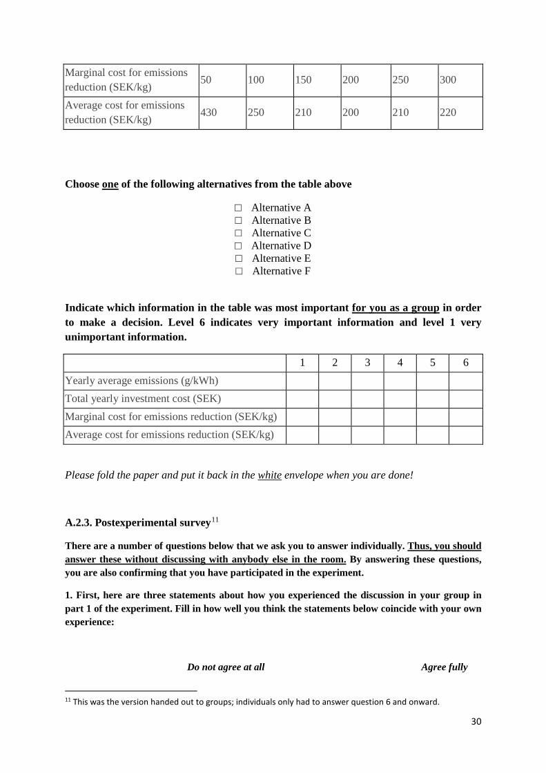
A.2.2. Instructions for the investment decision10

Below we will ask you to make an investment decision in your group. You can discuss within

the group, but we ask that you speak quietly in order not to disturb the other groups.

All investment decisions in the room are unique, and we ask that you therefore focus on the

decision that was assigned specifically to you.

Investment decision

We would like to ask you to assume a situation in which you are part of making a decision

about an environmental investment that a business will make in order to decrease its

environmental impact from environmentally hazardous emissions. There are 6 investment

options, each of which gives rise to specific emissions reductions. The table below shows the

different investment alternatives, including the effects each investment has on the emissions

of the business and investment costs.

When making your decision, you should take into account that the company needs to pay an

environmental tax equal to 250 SEK per kg each year for the emissions according to the table.

An investment that reduces the emissions causes a yearly investment cost but also means that

the company’s environmental tax expenses are reduced. The aim of the investment is to

generate the highest net return to the company.

Please indicate which investment alternative, Alt A to Alt F, you think the company should

choose. All alternatives A to F have the same economic lifetime.

Alt A Alt B Alt C Alt D Alt E Alt F

Yearly average emissions (g/kWh)

95 90 85 80 75 70

Total annual investment cost (SEK)

21 250 25 000 31 250 40 000 51 250 65 000

10 This was the version given to groups in the tax treatment.

30

Marginal cost for emissions reduction (SEK/kg)

50 100 150 200 250 300

Average cost for emissions reduction (SEK/kg)

430 250 210 200 210 220

Choose one of the following alternatives from the table above

□ Alternative A □ Alternative B □ Alternative C □ Alternative D □ Alternative E □ Alternative F

Indicate which information in the table was most important for you as a group in order to make a decision. Level 6 indicates very important information and level 1 very unimportant information.

1 2 3 4 5 6

Yearly average emissions (g/kWh) Total yearly investment cost (SEK) Marginal cost for emissions reduction (SEK/kg) Average cost for emissions reduction (SEK/kg)

Please fold the paper and put it back in the white envelope when you are done!

A.2.3. Postexperimental survey11

There are a number of questions below that we ask you to answer individually. Thus, you should answer these without discussing with anybody else in the room. By answering these questions, you are also confirming that you have participated in the experiment.

1. First, here are three statements about how you experienced the discussion in your group in part 1 of the experiment. Fill in how well you think the statements below coincide with your own experience:

Do not agree at all Agree fully

11 This was the version handed out to groups; individuals only had to answer question 6 and onward.

31

1 2 3 4

I participated actively in the discussion.

□ □ □ □

Everybody participated equally in the discussion.

□ □ □ □

One person took a leading role in the discussion.

□ □ □ □

2. Next, here are two questions about your collective decision in part 1 of the experiment. Fill in how well you think the statements below coincide with your own experience:


1 2 3 4

I would have made the same decision as the group even if I were on my own.

□ □ □ □

The discussion in the group changed my opinion.

□ □ □ □

The group thought that the task to choose an investment level was difficult.

□ □ □ □

3. Below are a couple of questions where we want to know how the members in your group influenced the discussion and your collective decision.

First, here is a figure of how you were seated in the room. Indicate the place where you sat with an X. Indicate the other two members in your group with an A and a B in the figure.

32

Figure

You and your group members’ placement:

Whiteboard and desk (in front of the hall)

□ □ □ 4. Now, here are three statements about member A in your group (according to your own figure above). Indicate how well the statements coincide with your own experience:


1 2 3 4

Member A had influence on our collective group decision.

□ □ □ □

Member A had a leading role in the group.

□ □ □ □

The group decision coincided with member A’s personal opinion.

□ □ □ □

5. Next, here are three statements about member B in your group (according to your own figure above). Indicate how well the statements coincide with your own experience:


1 2 3 4

Member B had influence on our collective group decision.

□ □ □ □

33

Member B had a leading role in the group.

□ □ □ □

The group decision coincided with member B’s personal opinion.

□ □ □ □

To sum up, here are a knowledge question and a couple of questions about your education and background.

6. Indicate which of the following general statements yields the highest net revenue for a company:

□ The company has chosen the investment with the lowest marginal cost in order to decrease the emissions.

□ The company has chosen the investment that implies that the average cost to decrease the emissions is equally high as the environmental tax (crowns per kg) for the emissions.

□ The company has chosen the investment that implies that the marginal cost to decrease the emissions is equally high as the environmental tax (crowns per kg) for the emissions.

□ The company has chosen the investment that gives the lowest average cost in order to decrease the emissions.

7. I have taken and finished courses at university level in:

□ microeconomics

□ environmental economics

□ mathematics and physics

8. How many finished (passed) university credits (uc) do you have in total if you would ask for a certificate from Ladok today?

□ 0–15 uc

□ 16–30 uc

□ 31–45 uc

□ 61–90 uc

□ 91–120 uc

□ >120 uc

34

□ 46–60 uc

9. How large do you think your share of ”pass with distinction” grades is for the courses you have finished?

□ 0–25%

□ 26–50%

□ 51–75%

□ 76–100%

10. In what year were you born? ____________

11. Sex:

□ Female □ Male □ Do not want to report/other

12. Specialization in your studies (if you are not sure, mark the specialization that you think you will specialize in):

□ Economics □ Business □ Logistics □ Social science environmental program with specialization in economics (SMIL) □ Other

13. How many of your group members did you know before?

□ 0 □ 1 □ 2

Thanks a lot for your participation!

By participating in the experiment, you have earned 40 crowns, but depending on your answer in part

1 of the experiment, you may have earned in total up to 100 crowns. We will willingly pay you via

Swish if you indicate your mobile phone number on the line below (write clearly):

My mobile phone number:

35

If you do not have access to or do not want to use Swish, you will be able to pick up your payment. If

you choose this alternative, you have to tear off the voucher below on this page. Take the voucher with

you for payment of the amount you have earned in the experiment. The payment will take place on the

following days and times at the student expedition (economics and statistics) on level 5, E-house:

February 1–3, 3 to 4 p.m.

If you want to know more about the experiment and which investment level gave the highest net

revenue, this information will be posted at the student expedition on level 5 in the E-house the first

two weeks of February.

36

Figure A.1. Photo from the experimental session on January 18, 2016

Documents

Environmental investment decisions: experimental evidence