Horizontal and Vertical Conflict: Experimental Evidence

NBER WORKING PAPER SERIES

HORIZONTAL AND VERTICAL CONFLICT:EXPERIMENTAL EVIDENCE

Sebastian GalianiCheryl Long

Camila NavajasGustavo Torrens

Working Paper 21857http://www.nber.org/papers/w21857

NATIONAL BUREAU OF ECONOMIC RESEARCH1050 Massachusetts Avenue

Cambridge, MA 02138January 2016

Cheryl Long appreciates the financial support from National Natural Science Foundation of China(Grant No. 71273217) and the Fundamental Research Funds for the Central Universities (Grant No.20720151001). The views expressed herein are those of the authors and do not necessarily reflect theviews of the National Bureau of Economic Research.

NBER working papers are circulated for discussion and comment purposes. They have not been peer-reviewed or been subject to the review by the NBER Board of Directors that accompanies officialNBER publications.

© 2016 by Sebastian Galiani, Cheryl Long, Camila Navajas, and Gustavo Torrens. All rights reserved.Short sections of text, not to exceed two paragraphs, may be quoted without explicit permission providedthat full credit, including © notice, is given to the source.

Horizontal and Vertical Conflict: Experimental EvidenceSebastian Galiani, Cheryl Long, Camila Navajas, and Gustavo TorrensNBER Working Paper No. 21857January 2016JEL No. D72,D74

ABSTRACT

Two types of political conflicts of interest pervade many of the world’s societies. A horizontal conflictof interest arises when different constituencies support different policies, while a vertical conflict ofinterest emerges when those in charge of running the government acquire and retain rents in the processof doing so. We experimentally explore the connections between the two. We identify two sets ofmodels that incorporate both types of conflicts: electoral models with endogenous rents, and common-agencymodels. We adapt these models to a laboratory setting and test their main theoretical predictions usingtwo experiments. In both cases we find support for the proposition that more intense horizontal conflictleads to higher rents, which is one of the theoretical predictions of the parametrized electoral and common-agencymodels that we have used.

Sebastian GalianiDepartment of EconomicsUniversity of Maryland3105 Tydings HallCollege Park, MD 20742and [email protected]

Cheryl LongDepartment of EconomicsColgate University13 Oak DriveHamilton, NY [email protected]

Camila NavajasUniversidad de San AndresBuenos Aires, [email protected]

Gustavo TorrensDepartment of EconomicsIndiana UniversityWylie Hall, 100 S Woodland AveBloomington, IN [email protected]

2

1. Introduction

The relationship between horizontal conflicts of interest (different groups support different

policies) and vertical conflicts of interest (those in charge of implementing policies acquire

and retain rents in the process of doing so) is one of the fundamental issues in political

economy. Although a great deal of progress has been made by focusing on one or the other

of these dimensions, the exact nature of the connections between the two is still one of the

hardest nuts that, both empirically and theoretically, has yet to be cracked in the realm of

political economy. Consider, for example, the relationship between inequality (a variable

commonly associated with horizontal conflict) and corruption (a variable usually associated

with vertical conflict). Corruption tends to be more widespread in more unequal societies.

Indeed, as Figure 11 shows, there is a positive correlation between inequality and corruption.

However, it could be misleading to read this correlation as evidence of a positive causal

relationship between income inequality and corruption. It is possible that very corrupt

practices are selectively affecting vulnerable groups and, hence, corruption is causing

inequality. Alternatively –and more likely– countries with good institutions are probably

better able to control government actions and induce a more egalitarian society. We

therefore need a theoretical framework in order to arrive at a better understanding of the

mechanisms underlying this correlation. We also need an exogenous source of variation in

one type of conflict in order to be able to estimate its effect on the other type of conflict.

Figure 1: Inequality and Corruption

Most models in political economy either emphasize one dimension of conflict or the other.

Electoral models typically stress horizontal conflict. Voters have heterogeneous preferences

regarding collective decisions, and candidates compete to attract their votes. Electoral

competition admits multiple variations depending on the assumptions made about the

number of issues on the ballot, the distribution of voters’ preferences, electoral rules, the

number of candidates, candidates’ preferences and the extent of uncertainty about voters’

preferences (see, for example, Roemer, 2001). Yet a common feature of most of these models

1 We use a database that includes 91 countries. The data on corruption was obtained from The World Justice Project (Rule of Law Index, Factor 2) while the data on inequality was obtained from The World Bank (Gini Index).

3

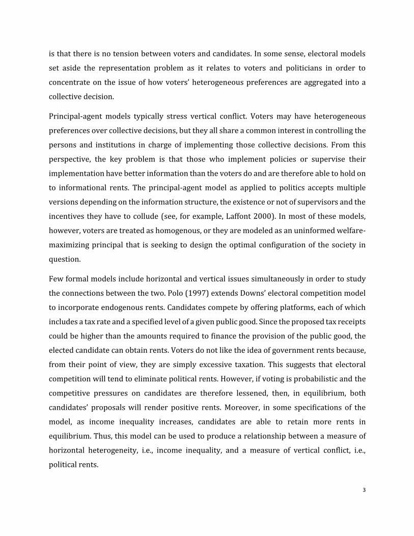
is that there is no tension between voters and candidates. In some sense, electoral models

set aside the representation problem as it relates to voters and politicians in order to

concentrate on the issue of how voters’ heterogeneous preferences are aggregated into a

collective decision.

Principal-agent models typically stress vertical conflict. Voters may have heterogeneous

preferences over collective decisions, but they all share a common interest in controlling the

persons and institutions in charge of implementing those collective decisions. From this

perspective, the key problem is that those who implement policies or supervise their

implementation have better information than the voters do and are therefore able to hold on

to informational rents. The principal-agent model as applied to politics accepts multiple

versions depending on the information structure, the existence or not of supervisors and the

incentives they have to collude (see, for example, Laffont 2000). In most of these models,

however, voters are treated as homogenous, or they are modeled as an uninformed welfare-

maximizing principal that is seeking to design the optimal configuration of the society in

question.

Few formal models include horizontal and vertical issues simultaneously in order to study

the connections between the two. Polo (1997) extends Downs’ electoral competition model

to incorporate endogenous rents. Candidates compete by offering platforms, each of which

includes a tax rate and a specified level of a given public good. Since the proposed tax receipts

could be higher than the amounts required to finance the provision of the public good, the

elected candidate can obtain rents. Voters do not like the idea of government rents because,

from their point of view, they are simply excessive taxation. This suggests that electoral

competition will tend to eliminate political rents. However, if voting is probabilistic and the

competitive pressures on candidates are therefore lessened, then, in equilibrium, both

candidates’ proposals will render positive rents. Moreover, in some specifications of the

model, as income inequality increases, candidates are able to retain more rents in

equilibrium. Thus, this model can be used to produce a relationship between a measure of

horizontal heterogeneity, i.e., income inequality, and a measure of vertical conflict, i.e.,

political rents.

4

Dixit, Grossman and Helpman (1997) extend the principal-agent model by introducing

multiple principals who try to influence a common agent. In a political context, the various

principals are usually interpreted as being special interest groups, and the common agent as

the government. This model is also capable of producing a relationship between horizontal

conflict and political rents. The idea is that as special interest groups have more conflicting

policy preferences, they are more willing to pay the government to move the chosen policy

in their preferred direction.

Summing up, there are two sets of formal models that incorporate both types of conflicts:

electoral models with endogenous rents, and common-agency models. Although they focus

on different channels (voting and lobbying, respectively), both models predict an increase in

rents as the intensity of horizontal conflict rises. We adapt these models to a laboratory

setting and test their theoretical predictions using two randomized experiments. In both

cases, we find support for the proposition that more intense horizontal conflict leads to

higher rents. The experiments also point to interesting directions for the refinement of these

models.

For our first experiment, we used a simple version of the electoral model with endogenous

rents presented in Polo (1997). The setup is as follows: There are 8 voters, each with an

initial endowment. There is a public good that is paid for by a proportional tax on voters’

endowments. Two candidates simultaneously propose a tax rate and a level of the public

good in question. The difference between tax receipts and the amount required to pay for

the public good is a political rent that will be collected by the candidate who wins the

election. Each voter receives extra points if a particular candidate wins the election. The

candidates only know the probability distribution of these extra points. We study four

treatments. In treatments 1 and 2, all voters have the same endowment, while in treatments

3 and 4, some voters have a larger endowment. In treatments 1 and 3, the variance of the

distribution of extra points is low, while in treatments 2 and 4, it is high. According to the

theoretical predictions of this model, we expect that, ceteris paribus, in those scenarios

where there is a higher level of inequality (treatments 3 and 4) or a higher level of electoral

uncertainty (treatments 2 and 4), the elected candidate obtains more rents.

5

We find evidence that supports the electoral model’s prediction that higher inequality leads

to higher political rents. We obtain a positive and significant effect on the rents of the elected

candidate when we compare treatment 1 with treatment 3 and when we compare treatment

2 with treatment 4. As is common in laboratory experiments (see, among others, Galiani,

Torrens and Yanguas 2014 for a discussion of this issue), the effects do not fit the model’s

predictions perfectly in quantitative terms. Indeed, the estimated effects of inequality on

rents are smaller than what our baseline model predicts. However, once we enrich the model

with more general risk preferences for the candidates, this gap narrows significantly.

Regarding electoral uncertainty, we do not find evidence that higher electoral uncertainty

induces higher rents. We also show that the candidates’ risk preferences are probably not

the reason of this result. It is more likely that some subjects did not fully understand how

electoral uncertainty affects electoral outcomes. Indeed, we show that, if we focus on

subjects who have a better understanding of the game (measured by the score in a quiz

administered before they play), we estimate a positive effect of electoral uncertainty on

rents.

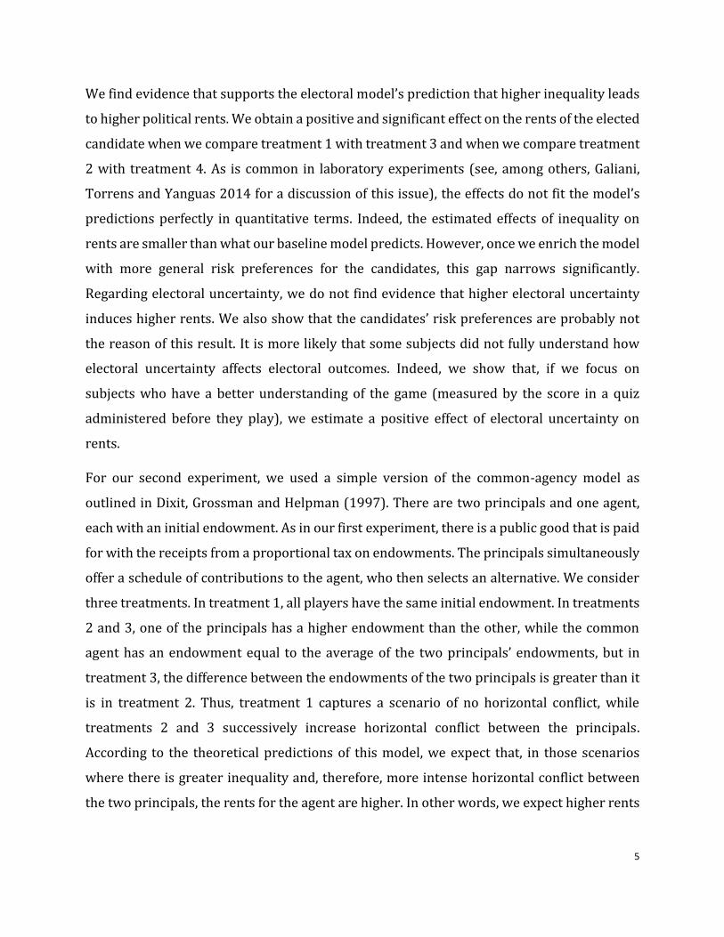
For our second experiment, we used a simple version of the common-agency model as

outlined in Dixit, Grossman and Helpman (1997). There are two principals and one agent,

each with an initial endowment. As in our first experiment, there is a public good that is paid

for with the receipts from a proportional tax on endowments. The principals simultaneously

offer a schedule of contributions to the agent, who then selects an alternative. We consider

three treatments. In treatment 1, all players have the same initial endowment. In treatments

2 and 3, one of the principals has a higher endowment than the other, while the common

agent has an endowment equal to the average of the two principals’ endowments, but in

treatment 3, the difference between the endowments of the two principals is greater than it

is in treatment 2. Thus, treatment 1 captures a scenario of no horizontal conflict, while

treatments 2 and 3 successively increase horizontal conflict between the principals.

According to the theoretical predictions of this model, we expect that, in those scenarios

where there is greater inequality and, therefore, more intense horizontal conflict between

the two principals, the rents for the agent are higher. In other words, we expect higher rents

6

for the agent in treatment 2 than for the agent in treatment 1 and higher rents for the agent

in treatment 3 than for the agent in treatment 2.

We find a positive effect for inequality on rents and payoffs when we compare treatment 1

with treatment 2 and treatment 2 with treatment 3. The effects, however, are smaller than

we would expect on the basis of the model’s predictions. The gap between observed and

predicted rents diminishes, but it does not disappear, when we focus on the group of subjects

who had a better understanding of the game, as measured by a quiz that we administered

before subjects began playing the rounds. We also show that the risk preferences of the

principals are probably not the underlying cause of these gaps.

Three areas of experimental studies are related to our work. First, there is a vast body of

experimental literature on electoral games. Second, there are many experimental works that

deal with principal-agent games, although not many focus on common-agency games.

Finally, there are several experiments that focus on contests and all-pay auctions.

Electoral Games. Our first experiment is related to the existing experimental literature on

electoral competition. McKelvey and Ordeshook (1990) surveyed experiments that examine

the hypothesis of platform convergence to the median preferred policy in the Downsian

model with purely office-motivated candidates. They considered different scenarios and

found that platforms converge even when voters are not fully informed. Morton (1993)

supplemented those studies by conducting a laboratory experiment to assess the hypothesis

that platforms diverge when candidates have policy preferences and there is uncertainty

about voters’ preferences. He found that platforms do indeed diverge but that, on average,

candidate positions are more convergent than the theory predicts, suggesting that the

subjects value winning independently of the expected payment. As in the works surveyed by

McKelvey and Ordeshook (1990), in our experiment, candidates do not have policy

preferences and, hence, their platforms are expected to converge. Analogous to the model in

Morton (1993), candidates are uncertain about voter’s preferences, which leads to positive

political rents in equilibrium. The reason, as discussed in Polo (1997), is that electoral

uncertainty lessens candidates’ incentives to reduce rents in order to capture more votes.

7

Other studies have experimented with variations of the standard electoral models. For

example, Aragones and Palfrey (2004) reported experimental results concerning the effects

of exogenous quality differences in the candidates (i.e., valence asymmetries) on the location

of the equilibrium policies in a one-dimensional policy space. In general, they found support

for theoretical predictions (e.g., the better candidate adopts more centrist policies than the

worse candidate does). Drouvelis, Saporiti and Vriend (2013) conducted a theoretical and

experimental study on the set of Nash equilibria of a classical one-dimensional electoral

game with two candidates who are interested in power and ideology, but who place values

on these two factors that are not necessarily identical. They also found that experimental

evidence supports the theoretical predictions. One difference between Aragones and Palfrey

(2004) and our experiment is that political rents in Polo (1997) work as endogenous quality

differences between the candidates. In Drouvelis, Saporiti and Vriend (2013), there is a more

opportunistic candidate who places more weight on winning the election. However, this is

not equivalent to vertical conflict between the candidates and the voters. More importantly,

none of these works provides predictions on the connection between horizontal

heterogeneity in voters’ preferences and candidates’ rents.

Principal-Agent Games. Our second experiment is related to several studies which have

experimented with principal-agent games. Many authors have conducted experiments with

principal-agent games in which there is a single principal. For example, Güth, Klose,

Königstein, and Schwalbach (1998) conducted an experiment with a multi-period principal-

agent game in which the principal has to offer linear profit-sharing contracts to the agent.

Ferh and Schmidt (2004) experimented with a two-task principal-agent game in which only

one task can be contracted out. Keser and Willinger (2007) conducted a laboratory

experiment with a principal–agent game involving moral hazard. Unfortunately, these

studies focus entirely on vertical conflict and cannot be used to gain an understanding of the

connections between horizontal and vertical conflicts.

The study conducted by Kirchsteiger and Prat (2001), who considered a common-agency

game, is closer to our work. The standard equilibrium concept for common-agency games is

a truthful equilibrium (Dixit, Grossman and Helpman, 1997). Kirchsteiger and Prat identify

a new class of equilibria, which they called “natural equilibria”. In their scenario, each

8

principal offers a positive contribution on at most one collective decision. They conducted a

laboratory experiment using a common-agency game for which the two notions of equilibria

predict a different equilibrium outcome. They found that the natural equilibrium is chosen

in 65% of the matches, while the truthful equilibrium is chosen in less than 5% of the

matches. This is not an issue in our experiment, since the existence of different types of

equilibria does not affect the comparative static predictions of the common-agency model,

which is the focus of our work.

Contests and All-Pay Auctions. Our experiments are also related to the literature on

contests and all-pay auctions. Hillman and Riley (1989) developed a model of politically

contestable rents and transfers in which all players make payments in order to exert political

influence, regardless of the final outcome. When players’ valuations are asymmetric, these

authors show that only the two players with the highest valuations enter the contest and

total expected payments are lower than the value of the politically allocated prize. Moreover,

as the ratio of the highest to the second-highest valuations increases, total expected

payments decrease (Corollary 1 in Hillman and Riley, 1989). Thus, in contrast to our

experiments, in the all-pay auction model of political influence, horizontal heterogeneity

reduces political rents. Several experimental studies with all-pay auction models have been

conducted. For example, Shogren and Baik (1991) reported on experimental behavior in

Tullock’s efficient rent-seeking game and found outcomes consistent with predicted

behavior and rent dissipation. Davis and Reilly (1994) reported the result of an experiment

with an all-pay auction game with four players. Potters, de Vries, and van Winden (1998)

reported on experiments that used both the Tullock probabilistic and highest-bid

(discriminating or all-pay auction) contest success functions. Gneezy and Smorodinsky

(2006) experimented with a repeated all-pay auction game with complete information,

perfect recall and common values. However, to the best of our knowledge, there is no

experimental study employing all-pay auction models that has tested the hypothesis that

expected political rents are lower when asymmetry in the two highest valuations increases.

The rest of this paper is organized as follows. In section 2, we focus on electoral games with

endogenous rents. We adapt a model developed by Polo (1997) to the laboratory setting and

test its main predictions. In section 3, we focus on common-agency games. We adapt a model

9

developed by Dixit, Grossman and Helpman (1997) to the laboratory setting and test its main

predictions. In section 4, we present our conclusions.

2. Electoral Competition with Endogenous Rents

In this section we study the connections between income inequality and political rents in the

context of electoral competition. In section 2.1, we briefly describe a model of electoral

competition with endogenous rents due to Polo (1997). In section 2.2, we use this model to

derive experimental treatments. In section 2.3, we describe the laboratory experiment. In

section 2.4, we show that subjects understood the electoral competition game and that the

randomization was balanced. In section 2.5, we present descriptive statistics and, in section

2.6, we formally test theoretical predictions using regression analyses and then discuss the

results.

Electoral Model with Endogenous Rents

Polo (1997) developed a model of electoral competition with endogenous rents. In the

model, there are 𝐼 citizens indexed by 𝑖 and two candidates who simultaneously decide on

their platforms. Let (𝜏𝑗 , 𝑔𝑗) be the platform proposed by candidate 𝑗 = 1,2 . A platform

consists of an income tax rate 𝜏𝑗 ∈ [0,1] and a per capita level of public goods 𝑔𝑗 ≥ 0. The

government budget constraint is given by:

𝜏𝑗𝑦 = 𝑔𝑗 +𝑟𝑗

𝐼.

where 𝑦 =∑ 𝑦𝑖𝐼

𝑖=1

𝐼 is the average income in the society and 𝑟𝑗 ≥ 0 are the rents that candidate

𝑗 will obtain if s/he is elected. If candidate 𝑗 wins the election, his/her payoff is given by:

𝑣𝐶,𝑗 = 𝑟𝑗 .

After the candidates select their platforms, all voters consider them and then vote for one of

the two candidates. The payoff for voter 𝑖 from the platform of candidate 𝑗 is given by:

𝑣𝑉,𝑖 = (1 − 𝜏𝑗)𝑦𝑖 + 𝐻 (𝑔𝑗) + 𝛽𝑗 ,

10

where 𝑦𝑖 is the income of voter 𝑖 and 𝐻 is a strictly increasing, strictly concave, twice

continuously differentiable function. 𝛽𝑗 is a valence or competence term. Assume that the

cumulative distribution of 𝛽 = 𝛽2 − 𝛽1is 𝐹. Thus, voter 𝑖 votes for candidate 1 if and only if:

(𝜏2 − 𝜏1)𝑦𝑖 + 𝐻 (𝑔1) − 𝐻 (𝑔2) > 𝛽.

The candidates know 𝐹, but they don’t observe the realization of 𝛽. In this case, candidate 1

wins the election with a probability given by:

𝐹(𝐻 (𝑔1) − 𝐻 (𝑔2) − (𝜏1 − 𝜏2)𝑦𝑚),

where 𝑦𝑚 is the median income. Hence, when the platforms are (𝜏1, 𝑔1) and (𝜏2, 𝑔2), the

expected payoff for candidates 1 and 2 are:

𝐄[𝑣𝐶,1] = 𝐼(𝜏1𝑦 − 𝑔1)𝐹(𝐻 (𝑔1) − 𝐻 (𝑔2) − (𝜏1 − 𝜏2)𝑦𝑚),

𝐄[𝑣𝐶,2] = 𝐼(𝜏2𝑦 − 𝑔2)[1 − 𝐹(𝐻 (𝑔1) − 𝐻 (𝑔2) − (𝜏1 − 𝜏2)𝑦𝑚)],

respectively. Polo (1999) provided conditions for 𝐹 under which this electoral game has a

unique symmetric Nash equilibrium. The following proposition summarizes the results.

Proposition 1. Suppose that 𝐹 satisfies all the conditions in assumption 1 in Polo (1997) and

1

2𝑦𝑚𝐹′(0)+

𝑔𝑚

𝑦< 1 . Then, the electoral competition game has a unique symmetric Nash

equilibrium characterized by 𝑔1 = 𝑔2 = 𝑔𝑚 and 𝜏1 = 𝜏2 =1

2𝑦𝑚𝐹′(0)+

𝑔𝑚

𝑦, where 𝐻′(𝑔𝑚) =

𝑦𝑚

𝑦. In equilibrium, each candidate wins with a probability of 1/2 and equilibrium rents are

given by 𝑟 = 𝐼𝑦

2𝑦𝑚𝐹′(0).

From Proposition 1 we can deduce a relationship between income distribution, electoral

uncertainty and political rents. Next, we develop a simple laboratory setting to test these

implications.

2.1. Treatments and Expected Outcomes

To implement the electoral competition game in the laboratory, we further specify 𝐻, 𝐹, 𝐼

and 𝑦𝑖. First, we impose that 𝐻(𝑔) = 2√𝑔 and 𝐹 is the normal distribution with mean 0 and

11

standard deviation 𝜎. Then, from Proposition 1, the equilibrium is given by 𝑔1 = 𝑔2 = 𝑔𝑚 =

𝑦

𝑦𝑚 and 𝜏1 = 𝜏2 =1+2√2𝜋𝜎

2√2𝜋𝜎𝑦𝑚 and equilibrium rents are given by 𝑟 = 𝐼√2𝜋𝜎𝑦

2𝑦𝑚 . Note that rents

increase with the uncertainty on the difference in candidate valance (higher 𝜎 ) and

inequality (higher 𝑦

𝑦𝑚). Second, supposing that there are eight voters and two candidates,

then, 𝑦 =∑ 𝑦𝑖8

𝑖=1

8. Third, keeping 𝑦 fixed, we induce a change in 𝑦𝑚 as follows. Let 𝑦𝑖 =

(1 −𝜃

3)

4𝑦

3 for 𝑖 = 1, 2, 3, 4, 5, 6 , and 𝑦𝑖 =

4𝜃𝑦

3 for 𝑖 = 7,8 . Then, selecting higher values of

𝜃, we produce more inequality, i.e., a reduction in 𝑦𝑚 with 𝑦 fixed. 2

For the experiment we set 𝑦 = 6 and consider four different treatments (see Table 1). Each

treatment differs in the level of inequality (a change in 𝜃) and/or the level of electoral

uncertainty (a change in 𝜎). Note that the theoretical predictions imply more rents before

higher levels of 𝜃 and/or 𝜎 . For our parametrizations, predicted rents triple when we

increase inequality (from T1 to T3 and from T2 to T4) and double when we increase electoral

uncertainty (from T1 to T2 and from T3 to T4).

Table 1: Treatments and Predicted Outcomes (Electoral Competition Game)

Treatments Inequality

(1)

Electoral Uncertainty

(2)

Theoretical Predictions

(3)

T1 𝜃 = 3/4 (None) 𝐺𝑖𝑛𝑖 = 0 𝜎 = 1/2 Low Rents (2√2𝜋)

T2 𝜃 = 3/4 (None) 𝐺𝑖𝑛𝑖 = 0 𝜎 = 1 Intermediate Low Rents (4√2𝜋)

T3 𝜃 = 9/4 (High) 𝐺𝑖𝑛𝑖 = 1/2 𝜎 = 1/2 Intermediate High Rents (6√2𝜋)

T4 𝜃 = 9/4 (High) 𝐺𝑖𝑛𝑖 = 1/2 𝜎 = 1 High Rents (12√2𝜋)

2.2. The Laboratory Experiment

The experiment was conducted between February and May 2015 at Xiamen University,

China. We recruited undergraduate and graduate students from any field of study and

conducted 10 sessions with 20 subjects each, for a total of 200 participants. Subjects were

allowed to participate in only one session. In each treatment, subjects played the electoral

2 In order to avoid corner solutions we need 𝑦 > 3 [

1+√2𝜋

√2𝜋] ≈ 4.20.

12

competition game with the values of 𝜃 and 𝜎 in Table 1. The experiment was programmed

and conducted using z-Tree software (Fischbacher, 2007). Each session lasted

approximately 105 minutes. The experiment proceeded as follows:

Assignment to Computer Terminals. Before each session began, the subjects were

randomly assigned to computer terminals.

Instructions. After the subjects were at their terminals, they received the instructions,

which were also explained by the organizers. Subjects then had time to read the instructions

on their own and ask questions. Appendix A.1 contains an English translation of the

instructions. This was the last opportunity that subjects had to pose any questions.

Quiz. In order to check whether participants understood the rules of the game, we asked

them to take a five-question quiz. The quiz was administered after we had given the

instructions, but before the rounds began. Subjects were paid approximately US$ 0.10 per

correct answer, but we never informed them which ones they had answered correctly. An

English translation of the quiz questions can be found in Appendix A.2.

Rounds. After the subjects finished the quiz, they began playing rounds, during which they

interacted only through a computer network using z-Tree software. Subjects played 20

rounds of the game. The first 4 rounds were for practice, and the last 16 rounds were for pay.

At the end of each round, the subjects received a summary of the decisions taken by both

themselves and their partners, including payoffs per round, their own accumulated payoffs

for paid rounds and nature’s decision.

Matching. There were 20 participants in each session. In each round, players were randomly

divided into two groups of 10 players. In odd rounds, one group played treatment 1 (𝑇1) and

the second group played treatment 3 (𝑇3). In even rounds, one group played treatment 2 (𝑇2)

and the other, treatment 4 (𝑇4). In each round, two players in each group were randomly

chosen to play the role of candidates. The rest played the role of voters. After roles were

assigned, each player was informed of his/her role.

Questionnaire. Finally, just before leaving the laboratory, all the subjects were asked to

complete a questionnaire, which was designed to enable us to test the balance across

13

experimental groups and to control for their characteristics in the econometric analysis.

Appendix A.3 contains an English translation of the questionnaire.

Payments. All subjects were paid privately, in cash. After the experiment was completed, a

password appeared on each subject’s screen. The subjects then had to present this password

to the person who was running the experiment in order to receive their payoffs. Subjects

earned, on average, US$ 8.87, which included a US$ 1.61 show-up fee, US$ 0.10 per correct

answer on the quiz and US$ 0.10 for each point they received during the paid rounds of the

experiment.

2.3. Understanding of the Game and Randomization Balance

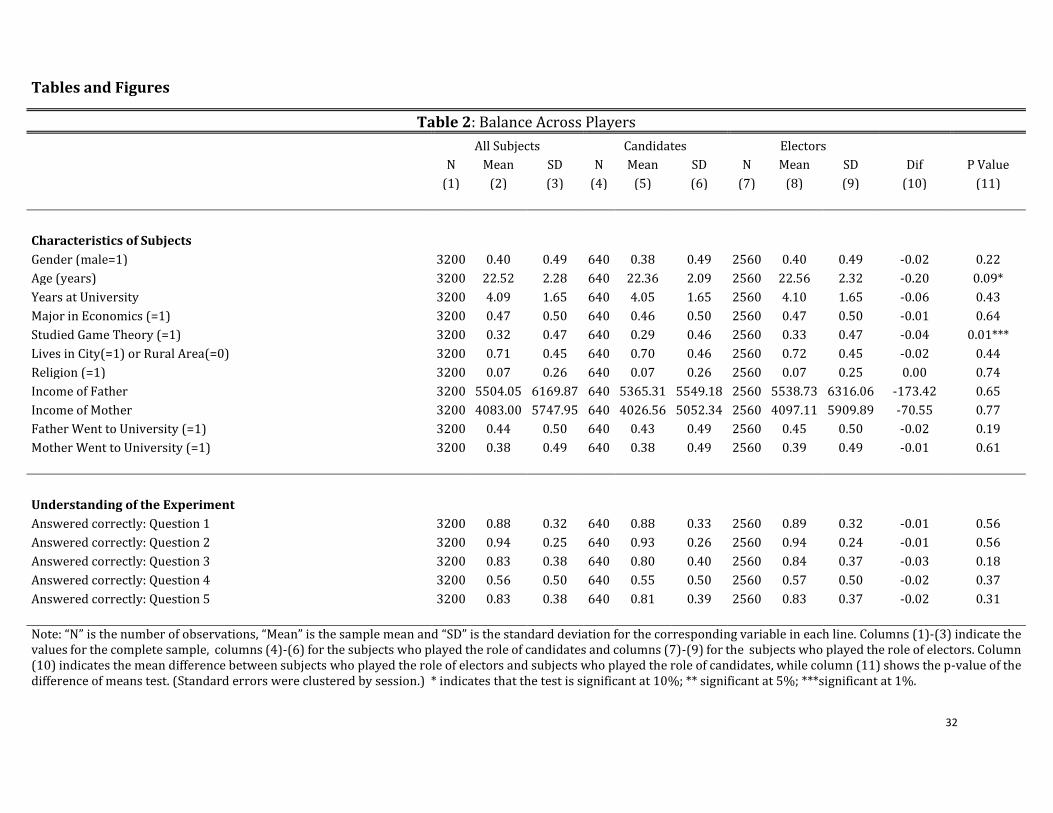
Table 2 shows that, on average, the subjects had a satisfactory understanding of the rules of

the game. In fact, 43% of the subjects answered all 5 questions correctly; 32.5% of them

answered 4 questions correctly; 15% got 3 questions right; 6% were able to answer only 2

questions correctly; 2.5% obtained a correct score on just 1 question; and, finally, 1% of the

subjects did not answer any of the questions correctly. In all, question 1 was answered

correctly by 88% of the subjects, question 2 by 94%, question 3 by 83%, question 4 by 56%

and question 5 by 83%. It therefore appears that the subjects found question 4 to be the most

difficult.

Table 2 also shows the randomization balance across player roles (candidates vs. voters).

Note that all characteristics and the understanding of the rules of the game are well balanced

across roles, as the mean difference between candidates and voters is not significantly

different from zero either for subject characteristics or for their understanding of the game.

The only exception is the variable that indicates if the subjects have studied game theory in

the past. However, this does not affect the average understanding of the game between

groups.

Table 2: Balance across Players

Tables 3 and 4, which compare the four treatments, show that all characteristics and levels

of understanding of the game were perfectly balanced between T1 and T3. In other cases,

there is a slight imbalance in some covariates such as gender, age, number of years at

14

university, whether the subjects have studied game theory or not, or whether they have a

religion. However, this did not affect the average understanding of the game between groups.

Tables 3 and 4: Balance Across Treatments I and II

2.4. Descriptive Analysis

Table 5 shows descriptive statistics for the main decisions taken by the subjects. For each

treatment, Table 5 indicates the total number of observations, the sample mean and the

standard deviation for the corresponding variable in each column. Column (1) reports the

income tax rate 𝜏; column (2) gives the per capita level of public goods 𝑔; column (3) shows

the payoff or rent of the elected candidate; column (4) lists the payoffs for the voters.

Table 5: Decisions across Treatments (Descriptive Statistics)

As predicted by the theory, tax rates and the level of public goods increase with inequality.

The average tax rates are 0.40 and 0.42 for T1 and T2 (the treatments with low levels of

inequality), while they are 0.81 and 0.73 points for T3 and T4 (the treatments with high

levels of inequality). On average, the levels of the public good are 1.63 and 1.77 points for T1

and T2 and 3.69 and 3.32 for T3 and T4. With higher taxes and more public goods when

inequality is high, what happens with rents is not exactly, clear, but, as the model predicts,

rents do increase with inequality. Column 3 in Table 5 shows that, on average, the elected

candidates obtained 6.79 points in T1 and 6.42 points in T2, while they got 9.40 and 8.67

points in T3 and T4, respectively. Contrary to theoretical predictions, on average, elected

candidates obtained less for treatments with higher levels of electoral uncertainty. Average

rents were lower in T2 than in T1 and in T4 than in T3.

2.5. Results

In order to formally test the hypothesis that higher levels of inequality and/or electoral

uncertainty lead to higher rents, we estimate the following regression model:

𝑅𝑒𝑛𝑡𝑒𝑐𝑖𝑝𝑠 = 𝛼 + 𝛽1𝐷𝑇 + 𝛽2𝑋𝑖𝑝𝑠 + ∑ 𝛽3𝐷𝛩𝑠

10

𝑠=1

+ 𝜀𝑖𝑝𝑠,

15

where 𝑖 indexes subjects, 𝑝 = 1,2,3, … ,16 indexes experimental rounds, and 𝑠 =

1,2,3, … ,10 indexes experimental sessions. 𝑅𝑒𝑛𝑡𝑒𝑐𝑖𝑝𝑠 is the dependent variable and indicates

the rents of the elected candidate 𝑖. The explanatory variable of interest is 𝐷𝑇, a dummy

variable indicating treatment status (𝑇𝑗 for 𝑗 = 1, 2, 3, 4). In some specifications, we also

include control variables. We control for individual characteristics 𝑋𝑖𝑝𝑠 (gender, age,

number of years at university, whether his or her major is in economics, whether s/he has

taken a course in game theory, whether s/he has a religion, the income of the father, the

income of the mother, whether his or her father has gone to university, whether his or her

mother has gone to university and the number of correct answers on the quiz) and for

session fixed effects (𝐷𝜃𝑠). According to our theoretical predictions, we should expect β̂1

to

be positive when comparing T1 with T2 and T3 with T4 (more electoral uncertainty in T2

and T4, respectively), T1 with T3 and T2 with T4 (more inequality in T3 and T4,

respectively), T1 with T4 (more electoral uncertainty and more inequality) and T2 with T3,

since there is an increase in inequality and a decrease in electoral uncertainty, but the effect

of inequality should be dominant. Table 6 shows the empirical results.

Table 6: Regressions

Economic Inequality and Rents. As expected, an increase in inequality leads to higher

rents. By comparing T1 with T3 and T2 with T4, we find a positive and statistically significant

estimate for all the specifications. The estimated increase in rents from T1 to T3 is 2.618

points (2.532 points when we include controls), while from T2 to T4 it is 2.256 points (2.239

points when we include controls). These estimations are consistent with the qualitative

comparative static predictions in Table 1.

Quantitatively, the estimations are lower than expected. Based on the data shown in Table 1,

we would expect that a move from no inequality to a Gini coefficient of ½ when the standard

deviation of valence is 1/2 (i.e., going from T1 to T3) induces an increase in rents of 4√2𝜋 ≈

10 points. The same variation in inequality when the standard deviation of valence is 1 (i.e.,

going from T2 to T4) should lead to an increase in rents of 8√2𝜋 ≈ 20 points. This suggests

that candidates are offering platforms that entail lower rents than predicted by the model.

One possible explanation is that the model assumes risk-neutral candidates. If candidates

16

are risk-averse, then we would expect them to be more willing to have a greater chance of

obtaining a low rent than a smaller chance of obtaining a high rent, which prompts them to

propose relatively lower rents. In order to see this, suppose that candidates have constant

relative risk aversion. Then, the expected payoff for candidate 1 is (an analogous expression

applies to candidate 2):

𝐄[𝑣𝐶,1] =[𝐼(𝜏1𝑦 − 𝑔1)]1−𝛾

1 − 𝛾𝐹(𝐻 (𝑔1) − 𝐻 (𝑔2) − (𝜏1 − 𝜏2)𝑦𝑚),

where 𝛾 is the coefficient of relative risk aversion. The first order conditions for candidate 1

become:

𝑦𝐹(𝐻 (𝑔1) − 𝐻 (𝑔2) − (𝜏1 − 𝜏2)𝑦𝑚) = 𝑦𝑚𝜏1𝑦 − 𝑔1

1 − 𝛾𝐹′(𝐻 (𝑔1) − 𝐻 (𝑔2) − (𝜏1 − 𝜏2)𝑦𝑚),

𝐹(𝐻 (𝑔1) − 𝐻 (𝑔2) − (𝜏1 − 𝜏2)𝑦𝑚) =𝜏1𝑦 − 𝑔1

1 − 𝛾𝐹′(𝐻 (𝑔1) − 𝐻 (𝑔2) − (𝜏1 − 𝜏2)𝑦𝑚)𝐻′(𝑔1).

If, in equilibrium, candidates converge to the same platform, we have 𝑔1 = 𝑔2 = 𝑔𝑚, where

𝐻′(𝑔𝑚) =𝑦𝑚

𝑦 and 𝑟1 = 𝑟2 = 𝐼

(1−𝛾)𝑦𝐹(0)

𝑦𝑚𝐹′(0). Thus, for our experiment 𝑟1 = 𝑟2 = 𝐼

(1−𝛾)√2𝜋𝜎𝑦

2𝑦𝑚=

(1 − 𝛾)3√2𝜋𝜎

(1−𝜃

3)

, which implies that going from T1 to T3 should induce an increase in rents of

(1 − 𝛾)4√2𝜋 ≈ (1 − 𝛾)10 points, while going from T2 to T4 should lead to an increase in

rents of (1 − 𝛾)8√2𝜋 ≈ (1 − 𝛾)20 points. There is a vast body of literature on the estimation

of coefficients of risk aversion. Holt and Laury (2002) employed a simple lottery choice

laboratory experiment that measures the degree of risk aversion. For low payoffs, they found

that the median 𝛾 is between 0.15 and 0.41 while, for higher payoffs, it is between 0.41 and

0.68. Many studies have estimated macro-finance models (see, for example, Byun el al.,

2007). Kim and Lee (2012) have reported a micro-econometric estimate of risk aversion

using survey responses to hypothetical lottery questions. They found that the constant

relative risk aversion parameter ranges from 0.6 to 0.8. In our model, if we consider 𝛾 ∈

[0.4,0.8], the predicted change in rents from T1 to T3 (T2 to T4) is between approximately 2

and 6 (4 and 12) points. Thus, introducing risk aversion significantly reduces the gap

between quantitative theoretical predictions and estimated effects.

17

It is also possible that candidates value winning the election independently of the expected

utility of rents. This, however, reduces predicted rents by a fixed amount in all treatments

and, hence, has no effect on the differences between two treatments. In order to see this,

suppose that candidates value the expected utility of endogenous and exogenous rents. Then,

the expected payoff of candidate 1 is given by:

𝐄[𝑣𝐶,1] =[𝜆𝐼(𝜏1𝑦 − 𝑔1) + (1 − 𝜆)𝑅]1−𝛾

1 − 𝛾𝐹(𝐻 (𝑔1) − 𝐻 (𝑔2) − (𝜏1 − 𝜏2)𝑦𝑚).

where 𝜆 ∈ [0,1] is the weight placed on endogenous rents and 𝑅 > 0 is exogenous rents, i.e.,

the utility of winning the election per se. Then, assuming that, in equilibrium, both candidates

offer the same platform, we have 𝑟1 = 𝑟2 = 𝐼(1−𝛾)𝑦𝐹(0)

𝑦𝑚𝐹′(0)− (

1−𝜆

𝜆) 𝑅 . Thus, the quantitative

predicted effect of a change in 𝑦𝐹(0)

𝑦𝑚𝐹′(0) on rents is not affected by the existence of candidates

who care about winning the election in and of itself.

Electoral Uncertainty and Rents. We did not find that an increase in electoral uncertainty

had any effect on rents. In both cases, when we compare T1 with T2 and T3 with T4, the

estimates are negative and not statistically significant. Thus, keeping inequality constant, an

increase in the standard deviation of valence from ½ to 1 does not produce any effect on

equilibrium rents. Note that neither risk preferences nor candidates who value winning the

election per se could be the explanation for this. Indeed, for any nonnegative and concave

utility function, if in equilibrium candidates converge to the same platforms, rents must be

increasing in electoral uncertainty. In order to see this, suppose that candidates have a

nonnegative and concave utility function 𝑣. Then, the expected payoff for candidate 1 is:

𝐄[𝑣𝐶,1] = 𝑣(𝐼(𝜏1𝑦 − 𝑔1))𝐹(𝐻 (𝑔1) − 𝐻 (𝑔2) − (𝜏1 − 𝜏2)𝑦𝑚).

In equilibrium, the first-order condition becomes 𝑣′ = 𝑣𝑦𝑚𝐹′(0)

𝑦𝐹(0)= 𝑣

2𝑦𝑚

𝑦√2𝜋𝜎, which implies:

𝑑𝑟

𝑑𝜎=

−2𝑦𝑚

𝑦√2𝜋𝜎2(𝑣′′𝑣 − (𝑣′)2)> 0.

A more plausible explanation is that subjects did not fully understand how electoral

uncertainty affects their electoral chances. In fact, if we focus on candidates who correctly

18

answered all the quiz questions, we obtain a positive, though nonsignificant, estimation

when we compare T1 with T2 (in all specification) and T3 with T4 (only for the specification

with no controls). Specifically, after restricting the sample to those candidates who scored

100% on the quiz, the estimated change in rents from T1 to T2 is 0.444 points (0.692 points

when we include controls), while from T3 to T4 it is 0.077 points (-0.229 points when we

include controls).

Inequality, Electoral Uncertainty and Rents. Finally, if we compare T1 with T4 (a scenario

with more inequality and more electoral uncertainty), we obtain the predicted outcome,

namely, a positive and statistically significant effect on rents, while, when we compare T2

with T3 (more inequality but less electoral uncertainty), we also obtain the positive

predicted effect on rents.

Summing up, we find evidence that supports the prediction of the electoral model with

endogenous rents that higher inequality leads to higher political rents. Quantitatively, the

effects are smaller than expected. The risk preferences of the candidates may be one of the

reasons for this gap. For the whole sample, we do not find evidence that higher electoral

uncertainty induces higher rents. However, when we restrict the analysis to subjects who

scored 100% on the quiz, we obtain a positive effect for electoral uncertainty on rents.

3. Common-Agency Game

In this section we study the connections between inequality and political rents in the context

of special interest politics. In section 3.1, we briefly describe a common-agency model

employed by Dixit, Grossman and Helpman (1997). In section 3.2, we use this model to

derive experimental treatments. In section 3.3, we describe the laboratory experiment. This

general description covers the experiment’s monetary payoffs, the number of sessions and

rounds, the matching procedure and the instructions received by the subjects. In section 3.4,

we show that subjects understood the common-agency game and that the randomization

was balanced. In section 3.5, we present descriptive statistics. Finally, in section 3.6, we

formally test theoretical predictions using regression analyses and discuss the results.

19

3.1. Common-Agency Model

Dixit, Grossman and Helpman (1997) developed a model in which several principals try to

influence a single agent. The principals are interpreted as special interest groups and the

agent as the government or a government agency in charge of selecting a policy. In particular,

suppose that the payoff for principal 𝑖 is given by:

𝑣𝑃,𝑖 = (1 − 𝜏)𝑦𝑃,𝑖 + 𝐻(𝑔) − 𝐶𝑖 ,

where 𝜏 ∈ [0,1] is the income tax rate; 𝑔 ≥ 0 is the level of per capita public goods; 𝑦𝑃,𝑖 is

the income of principal 𝑖 ; 𝐻 is a strictly increasing, strictly concave, twice continuously

differentiable function; and 𝐶𝑖 is the contribution that principal 𝑖 pays to the agent. The

government budget constraint is given by:

𝜏𝑦 = 𝑔,

where 𝑦 is the average income in the society concerned. The payoff for the agent is given by:

𝑣𝐴 = (1 − 𝜏)𝑦𝐴 + 𝐻(𝑔) + ∑ 𝐶𝑖

𝑖,

where 𝑦𝐴 is the income of the agent and ∑ 𝐶𝑖𝑖 is the contributions received by the agent.

The timing of events is as follows: first, the principals simultaneously announce a schedule

of contributions, i.e., a menu in which each principal specifies how much s/he pledges to pay

the agent if the policy that is implemented is 𝑔;3 then the agent selects a policy 𝑔.

Dixit, Grossman and Helpman (1997) showed that the game has a truthful equilibrium and

characterized this equilibrium. Proposition 2 summarizes the results.

Proposition 2. Suppose a common-agency game with only two principals. Then, the game

has a truthful equilibrium, which is characterized by:

i. The agent will implement 𝑔∗ given by 𝐻′(𝑔∗) = 1;

3A contribution schedule can also be seen as a take-it-or-leave-it offer whereby, if the agent implements 𝑔, then the principal pays a contribution of 𝐶.

20

ii. Principal 1 will pay the agent 𝐶1 = 3(𝑔∗ − 𝑔∗,2) (𝑦𝑃,2+𝑦𝐴

𝑦𝑃,1+𝑦𝑃,2+𝑦𝐴) − 2[𝐻(𝑔∗) − 𝐻(𝑔∗,2)],

where 𝑔∗,2 is given by:

2𝐻′(𝑔∗,2) = 3 (𝑦𝑃,2 + 𝑦𝐴

𝑦𝑃,1 + 𝑦𝑃,2 + 𝑦𝐴) ;

iii. Principal 2 will pay the agent 𝐶2 = 3(𝑔∗ − 𝑔∗,1) (𝑦𝑃,1+𝑦𝐴

𝑦𝑃,1+𝑦𝑃,2+𝑦𝐴) − 2[𝐻(𝑔∗) − 𝐻(𝑔∗,1)],

where 𝑔∗,1 is given by:

2𝐻′(𝑔∗,1) = 3 (𝑦𝑃,1+𝑦𝐴

𝑦𝑃,1+𝑦𝑃,2+𝑦𝐴).

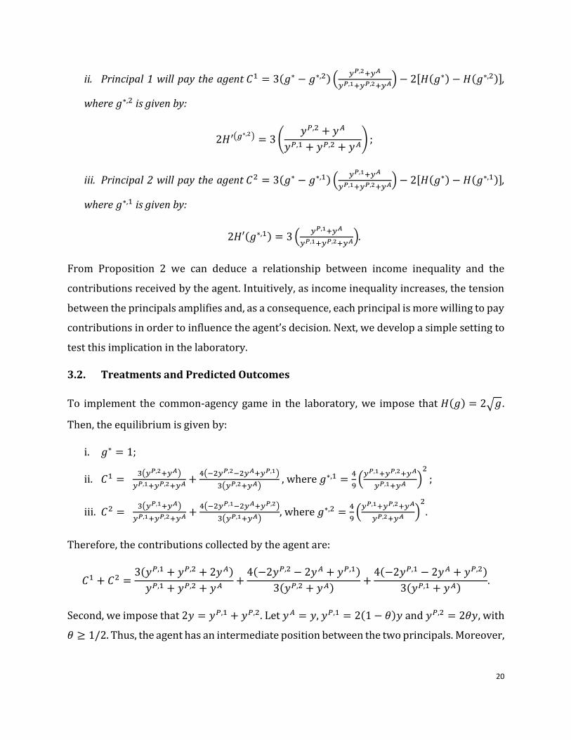
From Proposition 2 we can deduce a relationship between income inequality and the

contributions received by the agent. Intuitively, as income inequality increases, the tension

between the principals amplifies and, as a consequence, each principal is more willing to pay

contributions in order to influence the agent’s decision. Next, we develop a simple setting to

test this implication in the laboratory.

3.2. Treatments and Predicted Outcomes

To implement the common-agency game in the laboratory, we impose that 𝐻(𝑔) = 2√𝑔.

Then, the equilibrium is given by:

i. 𝑔∗ = 1;

ii. 𝐶1 = 3(𝑦𝑃,2+𝑦𝐴)

𝑦𝑃,1+𝑦𝑃,2+𝑦𝐴 +4(−2𝑦𝑃,2−2𝑦𝐴+𝑦𝑃,1)

3(𝑦𝑃,2+𝑦𝐴) , where 𝑔∗,1 =

4

9(

𝑦𝑃,1+𝑦𝑃,2+𝑦𝐴

𝑦𝑃,1+𝑦𝐴 )2

;

iii. 𝐶2 = 3(𝑦𝑃,1+𝑦𝐴)

𝑦𝑃,1+𝑦𝑃,2+𝑦𝐴 +4(−2𝑦𝑃,1−2𝑦𝐴+𝑦𝑃,2)

3(𝑦𝑃,1+𝑦𝐴), where 𝑔∗,2 =

4

9(

𝑦𝑃,1+𝑦𝑃,2+𝑦𝐴

𝑦𝑃,2+𝑦𝐴 )2

.

Therefore, the contributions collected by the agent are:

𝐶1 + 𝐶2 =3(𝑦𝑃,1 + 𝑦𝑃,2 + 2𝑦𝐴)

𝑦𝑃,1 + 𝑦𝑃,2 + 𝑦𝐴+

4(−2𝑦𝑃,2 − 2𝑦𝐴 + 𝑦𝑃,1)

3(𝑦𝑃,2 + 𝑦𝐴)+

4(−2𝑦𝑃,1 − 2𝑦𝐴 + 𝑦𝑃,2)

3(𝑦𝑃,1 + 𝑦𝐴).

Second, we impose that 2𝑦 = 𝑦𝑃,1 + 𝑦𝑃,2. Let 𝑦𝐴 = 𝑦, 𝑦𝑃,1 = 2(1 − 𝜃)𝑦 and 𝑦𝑃,2 = 2𝜃𝑦, with

𝜃 ≥ 1/2. Thus, the agent has an intermediate position between the two principals. Moreover,

21

a change in 𝜃 modifies income inequality, keeping average income fixed. Equilibrium

contributions are given by:

𝐶1 = (2𝜃 + 1) −8𝜃

(2𝜃 + 1) ,

𝐶2 = 2(1 − 𝜃) + 1 −8(1 − 𝜃)

2(1 − 𝜃) + 1 ,

𝐶1 + 𝐶2 = 4 −8𝜃

(2𝜃 + 1)−

8(1 − 𝜃)

3 − 2𝜃.

Note that 𝜕(𝐶1+𝐶2)

𝜕𝜃> 0 if 𝜃 > 1/2, i.e, when there is a higher level of inequality (higher 𝜃), the

agent gets more contributions. In other words, as the conflict between the two principals

heightens, the agent collects more rents. Moreover, in equilibrium, it is always the case that

𝑔∗ = 1. Then, the payoff for the agent also increases with income inequality. Formally, 𝜕𝑣𝐴

𝜕𝜃>

0 if 𝜃 > 1/2. For the experiment, we set 𝑦 = 2 and consider three different treatments,

which are summarized in Table 7.

Table 7: Treatments and Predicted Outcomes (Common-Agency Game)

Treatments Inequality

(1)

Theoretical Predictions

(2)

T1 𝜃 = 1/2 (None) 𝐺𝑖𝑛𝑖 = 0 Zero Rents for the Agent (𝐶1 + 𝐶2 = 0)

T2 𝜃 = 3/4 (Low) 𝐺𝑖𝑛𝑖 = 1/4 Intermediate Rents for the Agent (𝐶1 + 𝐶2 = 4/15)

T3 𝜃 = 1 (High) 𝐺𝑖𝑛𝑖 = 1/2 High Rents for the Agent (𝐶1 + 𝐶2 = 4/3)

Finally, to implement the common-agency game in the laboratory, we restrict the

contribution schedules that the principals can use to influence the agent. In particular, each

principal is allowed to select one contribution for each of the following tax rates 𝜏 =

0.25, 0.5, 0.75. Note that 𝜏 = 0.50 is the tax rate associated with the truthful equilibrium

(since, for the experiment, 𝑦 = 2, 𝜏 = 0.50 leads to 𝑔 = 1). Thus, we allow the principals to

select contributions for 𝜏 = 0.50 and two other tax rates symmetrically located to the left

and to the right of 𝜏 = 0.50. One key advantage of this formulation is that the agent can

collect contributions from both principals when selecting one policy. This is crucial in the

22

common-agency model, but it can be easily violated in the laboratory if more general

contribution schedules are permitted. Consider, for example, the biases that can emerge if

principals use any contribution schedule. Suppose that one principal plays the equilibrium

strategy, i.e., a positive contribution for 𝜏 = 0.50 and 0 otherwise, while the other principal

makes a slight calculation error and offers a positive contribution for 𝜏 = 0.49 and 0,

otherwise. In this case, the agent cannot collect both contributions. Another advantage of this

formulation is that the agent’s calculations are simpler. In particular, in order to evaluate his

or her options, the agent only needs to add up the two contributions for three possible tax

rates.

3.3. The Laboratory Experiment

The experiment was conducted between February and May 2015 at Xiamen University,

China. We recruited undergraduate and graduate students from any field of study. We

conducted 5 sessions with 18 subjects each, for a total of 90 participants. Subjects were

allowed to participate in only one session. In each treatment, subjects were asked to play a

common-agency game. The experiment was programmed and conducted using z-Tree

software (Fischbacher, 2007). Each session lasted approximately 90 minutes. The

experiment proceeded as follows:

Assignment to Computer Terminals. Before each session began, the subjects were

randomly assigned to computer terminals.

Instructions. After the subjects were at their terminals, they received the instructions. The

organizers then read out the instructions aloud, while the subjects read along. They were

instructed to ask questions throughout this period. Appendix B.1 contains an English

translation of the instructions. This was the last opportunity that subjects had to pose any

questions.




correct answer, but we never informed them which ones they had answered correctly. An

English translation of the quiz questions can be found in Appendix B.2.

23




At the end of each round, the subjects received a summary of the decisions taken by both

themselves and their partners, including payoffs per round and their own accumulated

payoffs for paid rounds.

Matching. In each round players were randomly divided into three groups of three players.

Each group played a common-agency game (with one group playing treatment 1, one group

treatment 2 and one group treatment 3). In each round and group, players were randomly

chosen to play the role of agent, principal 1 and principal 2. After roles were assigned, each

player was informed of his/her role.




Appendix B.3 contains an English translation of the questionnaire.






experiment.

3.4. Understanding of the Game and Randomization Balance

Table 8 shows that, on average, the subjects had a satisfactory understanding of the rules of

the game. In fact, 56.67% of the subjects answered all 5 questions correctly; 24.44% of them

answered 4 questions correctly; 11.11% of them got 3 questions right; 5.56% were able to

answer only 2 questions correctly; 1.11% obtained a correct score on just 1 question; and,

finally, 1.11% of the subjects did not answer any of the questions correctly. In all, question 1

was answered correctly by 76% of the subjects, question 2 by 74%, question 3 by 94%,

question 4 by 91% and question 5 by 91%.

24

Table 8 also shows the randomization balance across player roles (agent vs. principals). Note

that all characteristics and the understanding of the rules of the game are very well balanced

across roles, as the mean difference between agents and principals is not significantly

different from zero either for subject characteristics or for their understanding of the game.

The only exceptions are the variable that indicates if the subjects have studied game theory

in the past and the understating of question 1, but both of them are significant only at the

10% level.

Table 8: Balance across Players

Tables 9 and 10, which compare the three treatments, show that all characteristics and levels

of understanding of the game were perfectly balanced between T2 and T3. When we

compare T1 and T3, the only variable that is not balanced is a dummy that indicates whether

a subject lives in a town or in a rural area. The same thing happens when we compare T1 and

T3 but, in this case, the income of the father is not balanced either. However, this does not

affect the understanding of the game, for which there is no difference across the three

treatments.

Tables 9 and 10: Balance across Treatments I and II

3.5 Descriptive Analysis

Table 11 shows descriptive statistics for the main decisions taken by the subjects. For each

treatment, Table 11 indicates the total number of observations, the sample mean and the

standard deviation for the corresponding variable in each column. Column (1) reports the

income tax rate, τ ; column (2) gives the per capita level of public goods, g; column (3) shows

the rents of the agent, 𝐶1 + 𝐶2; column (4) lists the payoff for the agent, 𝑣𝐴; and column (5)

gives the payoff for the principals, 𝑣𝑃,1 and 𝑣𝑃,2.


As predicted by the theory, the tax rate and the level of public goods are very similar in all

the treatments. Indeed, the average tax rates are 0.48 in T1, 0.50 in T2 and 0.48 in T3, while

the average levels of the public good are 0.97, 0.99 and 0.96, respectively. Also, in line with

theoretical predictions, the rents collected by the agent increase with inequality. On average,

25

rents are 0.56 in T1, 0.59 in T2 and 0.78 in T3. The average payoff for the agent is also higher

in T3 (3.72) than in T1 (3.53) and T2 (3.54).

3.6. Results

We now formally test the theoretical predictions using regression analyses. In the context of

perfect experimental data, the identification of the effects of interest does not require the

inclusion of control variables. Moreover, the analysis is completely non-parametric, and we

therefore need only to compare the mean outcome differences across treatment groups.

Inferences could also be made non-parametric. Clustered standard errors are computed by

session.

In order to formally test the hypothesis that more inequality leads to higher rents, we

estimate the following regression models:

𝑅𝑒𝑛𝑡𝑎𝑔𝑖𝑝𝑠 = 𝛼 + 𝛽1𝐷𝑇 + 𝛽2𝑋𝑖𝑝𝑠 + ∑ 𝛽3𝐷𝛩𝑠

5

𝑠=1

+ 𝜀𝑖𝑝𝑠,

𝑃𝑎𝑦𝑜𝑓𝑓𝑎𝑔𝑖𝑝𝑠 = 𝛼 + 𝛽1𝐷𝑇 + 𝛽2𝑋𝑖𝑝𝑠 + ∑ 𝛽3𝐷𝛩𝑠

5

𝑠=1

+ 𝜀𝑖𝑝𝑠,

where 𝑖 indexes subjects, 𝑝 = 1, 2, 3 … 16 indexes experimental rounds, and 𝑠 = 1,2 … 5

indexes experimental sessions. 𝑅𝑒𝑛𝑡𝑎𝑔𝑖𝑝𝑠 indicates the rents collected by the agent, while

𝑃𝑎𝑦𝑜𝑓𝑓𝑎𝑔𝑖𝑝𝑠is the payoff for the agent. The explanatory variable of interest is 𝐷𝑇, a dummy

variable indicating treatment status ( 𝑇𝑗 for 𝑗 = 1, 2, 3 ). In some specifications, we also

include control variables. We control for individual characteristics 𝑋𝑖𝑝𝑠 (gender, age,

number of years at university, whether his or her major is in economics, whether s/he has

taken a course in game theory, whether s/he has a religion, the income of the father, the

income of the mother, whether his or her father has gone to university, whether his or her

mother has gone to university and the number of correct answers on the quiz) and for

session fixed effects (𝐷𝜃𝑠). According to our theoretical predictions, we should expect a

positive effect when comparing T1 with T2 and T2 with T3. Table 12 shows the estimations.

Table 12: Regressions

26

In all cases we estimate a positive effect for inequality on rents and payoffs. When we

compare T1 with T2, we obtain a positive but not statistically significant β̂1

. A move from no

inequality to an income distribution with a Gini coefficient of ¼ (i.e., going from T1 to T2)

induces an estimated increase in the rents collected by the agent of 0.034 points (0.0588

when we include controls). When we compare T2 with T3, we obtain a positive and

statistically significant effect. A move from an income distribution with a Gini coefficient of

¼ to another with ½ (i.e., going from T2 to T3) leads to an estimated increase in the rents of

0.185 points (0.152 if we include controls). Finally, when we compare T1 and T3, we obtain

a positive effect which is statistically significant only for the specification without controls.

A move from no inequality to an income distribution with a Gini coefficient of ½ (i.e., going

from T1 to T3) induces an estimated increase in the rents of 0.219 points (0.235 if we include

controls).

Quantitatively, these effects are smaller than the theoretical predictions. Indeed, as shown

in Table 7, we should expect an increase in rents of 4/15 ≈ 0.266 when we compare T1 with

T2, 4/3 − 4/15 ≈ 1.06 points when we compare T2 with T3 and 4/3 points when we

compare T1 with T3. Risk preferences do not seem to be the reason of these differences.

First, note that the agent does not face a risky choice. Once the principals have decided on

their contribution schedules, the agent selects one of three certain payoff options. Second,

the principals are faced with strategic uncertainty because when they decide on their

contributions, they do not know what contribution schedule has been selected by the other

principal. It is not clear how this should affect the quantitative theoretical predictions for T2

and T3. Nevertheless, it should definitely not affect our prediction for T1. When there is no

inequality, there is no conflict of interest and, hence, principals should not pay the agent to

implement a policy that s/he will pick anyway. However, as Table 11 shows, in T1, on

average, the agent collected 0.56 points.

One possible explanation for the gap between theoretical predictions and estimated effects

is that some subjects found the common-agency game to be too complicated. And, in fact, if

we focus on subjects who correctly answered all the quiz questions, the results are closer to

the theoretical predictions. As shown in columns (5)-(8) of Table 12, the estimated effects

are significantly bigger for all specifications. Specifically, estimated rents are 0.1318 points

27

higher in T2 than in T1 (0.179 points when we include controls), 0.297 points higher in T3

than in T2 (0.26 points when we include controls) and 0.435 points higher in T3 than in T1

(0.458 points when we include controls). Thus, focusing on subjects with the highest level of

understanding of the game reduces, but does not eliminate, the gap between the observed

behavior and theoretical predictions.

Summing up, we find evidence that supports the prediction of the common-agency model

that higher inequality leads to higher contributions. Quantitatively, the effects are smaller

than expected, but the gap narrows significantly when we focus on the subjects who had

perfect scores on the quiz.

4. Conclusions

The relationship between horizontal conflicts of interest and vertical conflicts of interest is

one of the fundamental questions in political economy. We have identified two sets of models

that incorporate both types of conflicts (electoral models with endogenous rents and

common-agency models), adapted them to a laboratory setting and used an experiment to

test their main theoretical predictions. For both models we have found evidence that

supports the prediction that higher inequality leads to higher political rents. We have also

extensively discussed different possible explanations for the quantitative differences

between the estimated effects and the models’ predictions.

Formal theory, cross-country correlations and laboratory evidence all suggest that we

should take the connections between horizontal and vertical conflicts seriously because they

have several important implications. At the macro level, they could help to account for the

persistence of corruption in some countries. Many developing countries are very unequal

societies with intense horizontal conflicts (see, among others, Lichbach, 1989; Cederman et

al., 2011; and Lupu and Pontusson, 2011). It should not be surprising that corruption and

other forms of political rents are ubiquitous in these countries. Some economic structures

are more likely to induce higher levels of heterogeneity in citizens’ preferences over

globalization and trade liberalization (see, for example, Galiani, Schofield and Torrens, 2014;

and Galiani and Torrens, 2014), and we can expect to observe more corruption and higher

political rents in countries with those economic structures. The intensity of horizontal

28

conflict tends to be higher in ethnolinguistically heterogeneous societies (see, for example,

Cederman et al., 2011). We should also expect higher political rents in countries troubled by

ethnic conflicts.

At the micro level, taking into account the relationship between horizontal and vertical

conflicts may help to improve the design of anti-corruption policies. Our impression is that

most of the recent literature on corruption has largely ignored this relationship (see, among

others, Warren, 2004; Tavits, 2007; and Chang and Golden, 2010). The emphasis is on

payment schemes, controls and audits, which are definitely good instruments for

discouraging corruption, but, in some cases, mitigating horizontal conflicts could be an

additional tool. Moreover, our findings indicate that we should assign scarce anti-corruption

resources, such as inspectors and auditors, to areas in which there are intense horizontal

conflicts.

We would like to close with a brief comment on the history of economic and political thought.

One simple way of classifying social theories –and even, perhaps, political philosophies– is

to gauge how much importance they place on horizontal and vertical conflict. At one extreme,

we have theories that emphasize horizontal conflict. For example, in Marxist thought, the

class struggle between workers and capitalists is the crucial social force, while the

government is just an instrument that is used by one class to impose its will on the others.

At the other extreme, we have theories that emphasize vertical conflict. For example, the

liberal school of thought tends to stress the importance of a limited government, the

separation of powers, and checks and balances. The weight that a social theory gives to

horizontal versus vertical issues can also influence the evaluation of public policies. For

example, a progressive social agenda that requires substantial political concentration to be

successful will probably receive the support of those that place more importance on

horizontal issues and be opposed by those who are more concerned with vertical problems.

Moreover, the surrounding political discourse will probably reflect the tension between

these perspectives. Groups that support the reform will argue that the opposition is trying

to protect the interests of privileged groups with the specter of a terrible leviathan. The

opposition will most certainly reply that the hidden agenda of the progressive reform is to

create such a leviathan, which will end up devouring even the well-intentioned features of

29

the reform. It would therefore seem that there is much to be gained from a better

understanding of the relationship between horizontal and vertical conflicts and the

associated trade-offs for society.

References

Aragones, E., and T. R. Palfrey (2004). “The effect of candidate quality on electoral

equilibrium: An experimental study”, American Political Science Review, vol. 98(01), pp. 77-

90.

Byun, S., S. Yoon, and B. Kang (2007). “Volatility spread on KOSPI 200 Index options and risk

aversion,” The Korean Journal of Finance, vol. 20, No. 3, pp. 97-126.

Cederman, L. E., N. B. Weidmann and K. S. Gleditsch (2011). “Horizontal inequalities and

ethnonationalist civil war: A global comparison”, American Political Science Review, vol.

105(03), pp. 478-495.

Chang, E., and M. A. Golden (2010). “Sources of corruption in authoritarian regimes”, Social

Science Quarterly, vol. 91(1), pp. 1-20.

Dixit, Avinash, Gene Grossman and Elhanan Helpman (1997).

“Common agency and coordination: General theory and application to government policy

making”, Journal of Political Economy, vol. 105, pp. 752-769.

Drouvelis, M., A. Saporiti and N. J. Vriend (2014). “Political motivations and electoral

competition: Equilibrium analysis and experimental evidence”, Games and Economic

Behavior, vol. 83, pp. 86-115.

Fehr, E., and K. M. Schmidt (2004). “Fairness and incentives in a multi‐task principal–agent

model”, The Scandinavian Journal of Economics, vol. 106(3), pp. 453-474.

Galiani S., N. Schofield and G. Torrens (2014). “Factor endowments, democracy and trade

policy divergence”, Journal of Public Economic Theory, vol. 16(1), pp. 119–156.

Galiani S., and G. Torrens (2014). “Autocracy, democracy and trade policy”, Journal of

International Economics, vol. 93(1), pp. 173-193.

30

Galiani, S., G. Torrens and M. L. Yanguas (2014). “The Political Coase Theorem: Experimental

evidence”, Journal of Economic Behavior & Organization, vol. 103, pp. 17-38.

Gneezy, U., and R. Smorodinsky (2006). “All-pay auctions: an experimental study”, Journal of

Economic Behavior & Organization, vol. 61(2), pp. 255-275.

Güth, W., W. Klose, M. Königstein and J. Schwalbach (1998). “An experimental study of a

dynamic principal–agent relationship”, Managerial and Decision Economics, vol. 19(4‐5), pp.

327-341.

Hillman, A. L., and J. Riley (1989). “Politically contestable rents and transfers”, Economics and

Politics, vol. 1, pp. 17-39.

Holt, C. A., and S. K. Laury (2002). “Risk aversion and incentive effects”, American Economic

Review, vol. 92(5), pp. 1644-1655.

Keser, C., and M. Willinger (2007). “Theories of behavior in principal–agent relationships

with hidden action”, European Economic Review, vol. 51(6), pp. 1514-1533.

Kim, Y. I., and J. Lee (2012). “Estimating risk aversion using individual-level survey data”,

Korean Economic Review, vol. 28(2), pp. 221-239.

Kirchsteiger, G., and A. Prat (2001). “Inefficient equilibria in lobbying”, Journal of Public

Economics, vol. 82(3), pp. 349-375.

Laffont, Jean Jacques (2000). Incentives and Political Economy, Oxford University Press.

Lupu, N., and J. Pontusson (2011). “The structure of inequality and the politics of

redistribution”, American Political Science Review, vol. 105(02), pp. 316-336.

McKelvey, R. D., and P. C. Ordeshook (1990). “A decade of experimental research on spatial

models of elections and committees”, Advances in the Spatial Theory of Voting, pp. 99-144.

Morton, R. B. (1993). “Incomplete information and ideological explanations of platform

divergence”, American Political Science Review, vol. 87(02), pp. 382-392.

Polo, Michele (1998). “Electoral competition and political rents”, No 144, Working Papers,

IGIER (Innocenzo Gasparini Institute for Economic Research), Bocconi University.

http://econpapers.repec.org/RePEc:igi:igierp:144

31

Potters, J., C. G. De Vries and F. Van Winden (1998). “An experimental examination of rational

rent-seeking”, European Journal of Political Economy, vol. 14(4), pp. 783-800.

Roemer, John E. (2001). Political Competition: Theory and Applications, Harvard University

Press, Cambridge, Massachusetts.

Shogren, J. F., and K. H. Baik (1991). “Reexamining efficient rent-seeking in laboratory

markets”, Public Choice, vol. 69(1), pp. 69-79.

Tavits, M. (2007). “Clarity of responsibility and corruption”, American Journal of Political

Science, vol. 51(1), pp. 218-229.

Warren, M. (2004). “What does corruption mean in a democracy?”, American Journal of

Political Science, vol. 48(2), pp. 328-343.

32

Tables and Figures

Table 2: Balance Across Players

All Subjects Candidates Electors

N Mean SD N Mean SD N Mean SD Dif P Value

(1) (2) (3) (4) (5) (6) (7) (8) (9) (10) (11)

Characteristics of Subjects

Gender (male=1) 3200 0.40 0.49 640 0.38 0.49 2560 0.40 0.49 -0.02 0.22

Age (years) 3200 22.52 2.28 640 22.36 2.09 2560 22.56 2.32 -0.20 0.09*

Years at University 3200 4.09 1.65 640 4.05 1.65 2560 4.10 1.65 -0.06 0.43

Major in Economics (=1) 3200 0.47 0.50 640 0.46 0.50 2560 0.47 0.50 -0.01 0.64

Studied Game Theory (=1) 3200 0.32 0.47 640 0.29 0.46 2560 0.33 0.47 -0.04 0.01***

Lives in City(=1) or Rural Area(=0) 3200 0.71 0.45 640 0.70 0.46 2560 0.72 0.45 -0.02 0.44

Religion (=1) 3200 0.07 0.26 640 0.07 0.26 2560 0.07 0.25 0.00 0.74

Income of Father 3200 5504.05 6169.87 640 5365.31 5549.18 2560 5538.73 6316.06 -173.42 0.65

Income of Mother 3200 4083.00 5747.95 640 4026.56 5052.34 2560 4097.11 5909.89 -70.55 0.77

Father Went to University (=1) 3200 0.44 0.50 640 0.43 0.49 2560 0.45 0.50 -0.02 0.19

Mother Went to University (=1) 3200 0.38 0.49 640 0.38 0.49 2560 0.39 0.49 -0.01 0.61

Understanding of the Experiment

Answered correctly: Question 1 3200 0.88 0.32 640 0.88 0.33 2560 0.89 0.32 -0.01 0.56





Note: “N” is the number of observations, “Mean” is the sample mean and “SD” is the standard deviation for the corresponding variable in each line. Columns (1)-(3) indicate the values for the complete sample, columns (4)-(6) for the subjects who played the role of candidates and columns (7)-(9) for the subjects who played the role of electors. Column (10) indicates the mean difference between subjects who played the role of electors and subjects who played the role of candidates, while column (11) shows the p-value of the difference of means test. (Standard errors were clustered by session.) * indicates that the test is significant at 10%; ** significant at 5%; ***significant at 1%.

33

Table 3: Balance Across Treatments I

All Subjects T1 T2 T3 T4

N Mean SD Mean SD Mean SD Mean SD Mean SD

(1) (2) (3) (4) (5) (6) (7) (8) (9) (10) (11)


Gender (male=1) 3200 0.40 0.49 0.40 0.49 0.38 0.49 0.40 0.49 0.42 0.49

Age (years) 3200 22.52 2.28 22.45 2.25 22.44 2.19 22.59 2.31 22.60 2.36

Years at University 3200 4.09 1.65 4.03 1.66 4.03 1.61 4.15 1.63 4.15 1.69

Major in Economics (=1) 3200 0.47 0.50 0.49 0.50 0.47 0.50 0.46 0.50 0.47 0.50

Studied Game Theory (=1) 3200 0.32 0.47 0.33 0.47 0.30 0.46 0.32 0.47 0.35 0.48

Lives in City(=1) or Rural Area(=0) 3200 0.71 0.45 0.69 0.46 0.73 0.45 0.74 0.44 0.70 0.46

Religion (=1) 3200 0.07 0.26 0.08 0.28 0.05 0.23 0.06 0.23 0.09 0.28

Income of Father 3200 5504.05 6169.87 5484.70 6038.45 5512.94 5868.41 5523.40 6304.16 5495.16 6462.80

Income of Mother 3200 4083.00 5747.95 4189.00 5971.39 3915.38 5213.99 3977.00 5519.05 4250.63 6236.82

Father Went to University (=1) 3200 0.44 0.50 0.44 0.50 0.44 0.50 0.45 0.50 0.45 0.50

Mother Went to University (=1) 3200 0.38 0.49 0.39 0.49 0.38 0.49 0.38 0.49 0.39 0.49


Answered correctly: Question 1 3200 0.88 0.32 0.88 0.32 0.89 0.31 0.89 0.31 0.88 0.33





Note: “N” is the number of observations, “Mean” is the sample mean and “SD” is the standard deviation for the corresponding variable in each line. Columns (1)-(3) indicate the values for the complete sample, columns (4)-(6) for the subjects who played treatment 1, columns (6)-(7) for those who played treatment 2, columns (8)-(9) for those who played treatment 3 and columns (10)-(11) for those who played treatment 4. Note that there were 800 observations of each of the variables in each treatment.

34

Table 4: Balance Across Treatments II

T1/T2 T2/T3 T3/T4 T1/T3 T1/T4 T2/T4

(1) (2) (3) (4) (5) (6)


Gender (male=1) 0.02* -0.02 -0.02* 0.00 -0.02* -0.02*

Age (years) 0.01 -0.14* -0.01 -0.13 -0.14* -0.15

Years at University 0.00 -0.12* 0.00 -0.12 -0.12* -0.12

Major in Economics (=1) 0.01 0.02 -0.01 0.03 0.02 0.00

Studied Game Theory (=1) 0.03 -0.02 -0.03 0.01 -0.02 -0.04**

Lives in City(=1) or Rural Area(=0) -0.03 -0.01 0.03 -0.04 -0.01 0.02

Religion (=1) 0.03*** 0.00 -0.03*** 0.03 0.00 -0.03**

Income of Father -28.24 -10.46 28.24 -38.70 -10.46 17.77

Income of Mother 273.63 -61.63 -273.63 212.00 -61.63 -

335.25

Father Went to University (=1) 0.00 -0.01 0.00 -0.02 -0.01 -0.01

Mother Went to University (=1) 0.02 0.00 -0.02 0.02 0.00 -0.02


Answered correctly: Question 1 -0.01 0.00 0.01 -0.01 0.00 0.01

Answered correctly: Question 2 0.00 0.00 0.00 0.00 0.00 0.00

Answered correctly: Question 3 -0.03 0.00 0.03 -0.04 -0.01 0.03

Answered correctly: Question 4 0.00 -0.01 0.00 -0.01 -0.01 -0.01

Answered correctly: Question 5 -0.01 0.00 0.01 -0.01 0.00 0.02

Note: Each entry indicates the mean difference between the two treatments in the column for the corresponding variable in each line. * indicates that the difference of means test is significant at 10%; ** significant at 5%; *** significant at 1%. Standard errors were clustered by session.

35


τ g vc vE

(1) (2) (3) (4)

T1

N 80 80 80 640

Mean 0.41 1.63 6.79 6.12

SD 0.17 0.91 4.08 0.73

T2

N 80 80 80 640

Mean 0.43 1.77 6.42 6.31

SD 0.20 1.06 3.85 0.83

T3

N 80 80 80 640

Mean 0.81 3.69 9.40 5.00

SD 0.24 1.41 4.63 2.24

T4

N 80 80 80 640

Mean 0.73 3.32 8.67 5.39

SD 0.28 1.46 4.59 2.87 Note: Column (1): Income tax rate, τ. Column (2): per capita level of public goods, g. Column (3): Payoff for the elected candidate, vc. Column (4): Payoff for the electors, vE.

36

Table 6: Regressions (Rents of the Elected Candidate)

(1) (2)

More Electoral Uncertainty

(a) Treatment 1 (=0) vs Treatment 2 (=1)

-0.368 -0.648

S.e. clustered by session (0.304) (0.355)

R-squared 0.002 0.072

N 160 160

(b) Treatment 3 (=0) vs Treatment 4 (=1)

-0.730 -0.781


R-squared 0.006 0.066

N 160 160

More Inequality

(c) Treatment 1 (=0) vs Treatment 3 (=1)

2.618** 2.532**


R-squared 0.084 0.176

N 160 160

(d) Treatment 2 (=0) vs Treatment 4 (=1)

2.256*** 2.239***


R-squared 0.067 0.161

N 160 160

𝛽1̂

𝛽1̂

𝛽1̂

𝛽1̂

37

Table 6: Regressions (Rents of the Elected Candidate)

More Electoral Uncertainty and Inequality

(e) Treatment 1 (=0) vs Treatment 4 (=1)

1.888** 1.654*


R-squared 0.046 0.140

N 160 160

More Inequality, Less Electoral Uncertainty

(f) Treatment 2 (=0) vs Treatment 3 (=1)

2.986** 3.109***


R-squared 0.111 0.248

N 160 160

Controls No Yes Note: * significant at 10%; ** significant at 5%; *** significant at 1% (using standard errors clustered by session). Controls: (i) Individual characteristics: gender, age, years at university, whether his/her major is economics, whether s/he has ever taken a course in game theory, whether s/he lives in a city, whether s/he has a religion, income of the father, income of the mother, whether his/her father has gone to university, whether his/her mother has gone to university; (ii) Level of understanding of the game: number of correct answers; and (iii) fixed effects, by session.

𝛽1̂

𝛽1̂

38

Table 8: Balance across Players’ Roles

All Subjects Agent Principals

N Mean SD N Mean SD N Mean SD Dif P Value

(1) (2) (3) (4) (5) (6) (7) (8) (9) (10) (11)


Gender (male=1) 1440 0.43 0.50 480 0.44 0.50 960 0.43 0.50 0.00 0.91

Age (years) 1440 22.36 2.34 480 22.33 2.34 960 22.37 2.33 -0.04 0.66

Years at University 1440 3.94 1.64 480 3.90 1.60 960 3.96 1.67 -0.06 0.34

Major in Economics (=1) 1440 0.39 0.49 480 0.39 0.49 960 0.39 0.49 0.00 0.94

Studied Game Theory (=1) 1440 0.28 0.45 480 0.31 0.46 960 0.26 0.44 0.04 0.09*

Lives in City(=1) or Rural Area(=0) 1440 0.70 0.46 480 0.68 0.47 960 0.71 0.45 -0.03 0.45

Religion (=1) 1440 0.14 0.35 480 0.17 0.37 960 0.13 0.34 0.04 0.17

Income of Father 1440 11366.67 52159.70 480 13017.29 59603.02 960 10541.35 48019.97 2475.94 0.43

Income of Mother 1440 9998.89 52676.93 480 11154.17 59832.75 960 9421.25 48730.07 1732.92 0.58

Father Went to University (=1) 1440 0.41 0.49 480 0.39 0.49 960 0.42 0.49 -0.03 0.49

Mother Went to University (=1) 1440 0.34 0.48 480 0.32 0.47 960 0.36 0.48 -0.04 0.38

39

Table 8: Balance across Players’ Roles


Answered correctly: Question 1 1440 0.76 0.43 480 0.74 0.44 960 0.77 0.42 -0.03 0.07*

Answered correctly: Question 2 1440 0.74 0.44 480 0.74 0.44 960 0.74 0.44 0.00 0.97




Note: “N” is the number of observations, “Mean” is the sample mean and “SD” is the standard deviation for the corresponding variable in each line. Columns (1)-(3) indicate the values for the complete sample, columns (4)-(6) for the subjects who played the role of agent and columns (7)-(9) for the subjects who played the role of principals. Entries in column (10) indicate the mean difference between subjects who played the role of agent and those who played the role of principals, while column (11) shows the p-value of the difference of means test. (Standard errors were clustered by session.)

* indicates that the test is significant at 10%; ** significant at 5%; ***significant at 1%.

40

Table 9: Balance Across Treatments I

All Subjects T1 T2 T3

N Mean SD Mean SD Mean SD Mean SD

(1) (2) (3) (4) (5) (6) (7) (8) (9)


Gender (male=1) 1440 0.43 0.50 0.41 0.49 0.46 0.50 0.43 0.50

Age (years) 1440 22.36 2.34 22.44 2.45 22.16 2.10 22.47 2.44

Years at University 1440 3.94 1.64 3.97 1.64 3.90 1.62 3.97 1.67

Major in Economics (=1) 1440 0.39 0.49 0.40 0.49 0.39 0.49 0.37 0.48

Studied Game Theory (=1) 1440 0.28 0.45 0.28 0.45 0.26 0.44 0.29 0.45

Lives in City(=1) or Rural Area(=0) 1440 0.70 0.46 0.76 0.43 0.66 0.47 0.68 0.47

Religion (=1) 1440 0.14 0.35 0.15 0.36 0.14 0.35 0.14 0.35

Income of Father 1440 11366.67 52159.70 11360.63 50533.32 12050.00 55377.89 10689.38 50517.40

Income of Mother 1440 9998.89 52676.93 9790.83 51050.55 10429.79 55773.11 9776.04 51176.98

Father Went to University (=1) 1440 0.41 0.49 0.42 0.49 0.41 0.49 0.40 0.49

Mother Went to University (=1) 1440 0.34 0.48 0.35 0.48 0.37 0.48 0.32 0.47


Answered correctly: Question 1 1440 0.76 0.43 0.75 0.43 0.74 0.44 0.78 0.42





Note: “N” is the total number of observations, “Mean” is the sample mean and “SD” is the standard deviation for the corresponding variable in each line. Columns (1)-(3) indicate the values for the complete sample, columns (4)-(5) for the subjects who played treatment 1, columns (6)-(7) for those who played treatment 2 and columns (8)-(9) for those who played treatment 3. Note that there were 480 observations of each of variable in each treatment.

41

Table 10: Balance Across Treatments II

T1/T2 T2/T3 T1/T3

(1) (2) (3)


Gender (male=1) -0.05 0.03 -0.01

Age (years) 0.27 -0.30 -0.03

Years at University 0.07 -0.07 0.00

Major in Economics (=1) 0.01 0.02 0.03

Studied Game Theory (=1) 0.02 -0.03 0.00

Lives in city(=1) or Rural Area(=0) 0.09** -0.01 0.08***

Religion (=1) 0.01 0.00 0.01

Income of Father -689.38 1360.63 671.25***

Income of Mother -638.96 653.75 14.79

Father Went to University (=1) 0.01 0.00 0.02

Mother Went to University (=1) -0.02 0.05 0.03


Answered correctly: Question 1 0.01 -0.04 -0.03

Answered correctly: Question 2 -0.01 -0.01 -0.02

Answered correctly: Question 3 -0.02 0.03 0.01

Answered correctly: Question 4 0.02 -0.01 0.01

Answered correctly: Question 5 0.02 -0.03 -0.01

Note: Each entry indicates the mean difference between the two treatments in the column for the corresponding variable in each line. * indicates that the difference of means test is significant at 10%; **significant at 5%; *** significant at 1%. Standard errors were clustered by session.

42


Τ g r vA vP

(1) (2) (3) (4) (5)

T1

N 480 480 160 160 320

Mean 0.48 0.97 0.56 3.53 3.70

SD 0.15 0.30 0.93 0.93 0.59

T2

N 480 480 160 160 320

Mean 0.50 0.99 0.59 3.54 3.65

SD 0.21 0.43 0.85 0.85 0.72

T3

N 480 480 160 160 320

Mean 0.48 0.96 0.78 3.72 3.55

SD 0.23 0.45 0.87 0.87 1.17

Note: Column (1): Income tax rate, τ. Column (2): per capita level of public goods, g. Column (3): Rents of the agent, r. Column (4): Payoff for the agent, vA. Column (5): Payoff for the principals, vp.

43

Table 12: Regression Analysis (Rents and Payoff for the Agent)

(1) (2) (3) (4) (5) (6) (7) (8)

Treatment 1 (=0) vs Treatment 2 (=1)

0.0341 0.0588 0.00939 0.0337 0.138 0.179 0.110 0.152

S.e. clustered by session (0.0792) (0.0799) (0.0794) (0.0800) (0.0831) (0.0844) (0.0837) (0.0860)

R-squared 0.000 0.036 0.000 0.035 0.007 0.109 0.004 0.105

N 320 320 320 320 185 185 185 185


0.185* 0.152* 0.178** 0.144* 0.297 0.260 0.289 0.251


R-squared 0.012 0.074 0.011 0.074 0.026 0.147 0.024 0.147

N 320 320 320 320 179 179 179 179


0.219* 0.235 0.188* 0.202 0.435** 0.458** 0.399** 0.420**


R-squared 0.015 0.048 0.011 0.047 0.057 0.149 0.048 0.144

N 320 320 320 320 180 180 180 180

Controls? No Yes No Yes No Yes No Yes Note: * significant at 10%; ** significant at 5%; *** significant at 1% (using standard errors clustered by session). Controls: Individual

characteristics: gender, age, years at university, whether his/her major is economics, whether s/he has ever taken a course in game theory,

whether s/he lives in a city, whether s/he has a religion, income of the father, income of the mother, whether his/her father has gone to

university, whether his/her mother has gone to university (ii) Level of understanding of the game: number of corrected answers and (iii)

Fixed effects by session. Columns (1), (2), (5) and (6) have as a dependent variable the rents of the agent and Columns (3), (4), (7) and (8)

have as a dependent variable the payoff of the agent. Columns (1)-(4) include all the subjects while columns (5)-(8) include only subjects

who answered correctly all the questions of the quiz.

𝛽1̂

𝛽1̂

𝛽1̂

44

Figure 1: Corruption and Inequality across Countries

45

Online Appendix A: Electoral Competition Game

In this appendix we describe the experimental design of the electoral competition game.

We used the following procedure.

Assignment to Computer Terminals. Before each session began, subjects were randomly

assigned to computer terminals.



instructed to ask questions throughout. Appendix A.1 contains an English translation of the

instructions. This was the last opportunity that subjects had to pose questions.



instructions, but before the rounds began. Subjects were paid per correct answer, but we

never informed them which ones they had correctly answered. An English translation of the

quiz questions can be found in Appendix A.2.




At the end of each round, subjects received a summary of the decisions taken by both



Matching. There were 20 participants in each session. In each round players were randomly

divided in two groups of 10 players. In odd rounds, one group played treatment 1 (𝑇1) and

the second group played treatment 3 (𝑇3). In even rounds, one group played treatment 2 (𝑇2)

and the other treatment 4 (𝑇4). In each round, two players in each group were randomly

chosen to play the role of candidates. The rest played the role of voters. After roles were

assigned, each player was informed of his/her role.



46


Appendix A.3 contains an English translation of the questionnaire.




earned, on average, US$ 8.87, which included a US$1.61 show-up fee, US$0.10 per correct

answer on the quiz, and US$ 0.10 for each point they received during the paid rounds of the

experiment.

A.1. Script for Instructions (Electoral Competition)

We would like to welcome everyone to this experiment. This is an experiment in decision-

making, and you will be paid, in cash, for your participation at the end of the experiment.

Different subjects may earn different amounts. What you earn depends partly on your

decisions, partly on the decisions of others and partly on chance.

The entire experiment and all interactions between participants will be conducted through

the computer terminals. It is very important for you not to talk or to try to communicate with

other subjects in any way during the experiment.

At your workstation, you will find a pencil, a sheet of paper with instructions and scratch

paper. During the experiment you can use the scratch paper to make calculations.

We will now start with a brief instruction period. During the instruction period, you will be

given a complete description of the experiment. If you have any questions during this period,

please raise your hand and your question will be answered so that everyone can hear it. If

any difficulties arise after the experiment has begun, raise your hand, and one of the persons

conducting the experiment will come to assist you.

You are one of 20 students who have been invited to take part in this experiment. In each

round you will be randomly assigned to one of two groups, consisting of 10 persons each.

You will then play the computer game, which will appear on the screen, with the members

of your group. At the beginning of each round, the parameters of the game will appear on the

screen, as will the time allotted for the game. At the end of the round, you will be informed

47

of the result of the game, the points you have earned during that round and the points you

have accumulated so far. In the next round, all players will again be randomly assigned to

one of the two new groups of 10 people each.

The experiment you are participating in is broken down into four unpaid practice rounds

and twelve paid rounds. At the end of the last round, you will be paid the total amount that

you have accumulated during the course of the last twelve rounds. Your profit is

denominated in POINTS. Your RMB profit is determined by multiplying your earnings in

points by a conversion rate. In this experiment, the conversion rate is RMB 0.6 to 1 point.

Everyone will be paid in private and you are under no obligation to tell others how much you

earned.

Please read the instructions that you will find by your desktop carefully. You have 10

minutes. Please, remember that if you have any questions, you should ask them aloud.

Instructions (Electoral Competition)

You will be playing in a group with 9 other participants. The computer will randomly select

the players that will be in each group in every round.

In each round the computer will also randomly assign you a role. You may be either one of

the two “proposers” or one of the eight “electors” who must choose between the two

proposals. All participants have the same chance of playing each role.

Six of the electors get 𝑦𝑖 = (1 −𝜃

3)

4𝑦

3 points, while the other two electors get 𝑦𝑖 =

4𝜃𝑦

3

points. Everybody knows this. That is, you will be informed of your role and the points that

each elector got.

If you are one of the proposers, you will be asked to make a proposal. A proposal consists of

two decisions. First, you have to decide what fraction of the electors’ points that you propose

to take from them. Second, you must decide what you’re going to do with these points. You

can keep them, you can use them to benefit electors or you can choose any other option in

between those alternatives. For example, if you propose to take a fraction 𝜏 of the points and

transfer 𝑔 points to each elector, you will get 𝑟 = 𝜏 ∑ 𝑦𝑖8𝑖=1 − 8𝑔 points and each elector will

48

get (1 − 𝜏)𝑦𝑖 + 2√𝑔 points (only, of course, if your proposal is the one that is selected). The

other proposer will also make a proposal at the same time. You have 90 seconds to make

your decision. When you select an option, please press the "Next" button. If, after 90 seconds,

you have not selected an option, the computer will do it for you at random.

After both proposers make their proposals, the computer will randomly select the extra

points that an elector gets when a proposer wins. Every elector gets 𝛽1 extra points if

proposer 1 wins the election and 𝛽2 extra points if proposer 2 wins the election. The

expected extra points that each elector gets is the same for both proposers. In particular,

𝛽1 − 𝛽2 = �̅�𝑘 > 0 with probability 𝑝𝑘 , 𝛽1 − 𝛽2 = −�̅�𝑘 with probability 𝑝𝑘 and 𝛽1 − 𝛽2 = 0

with probability 1 − 2 ∑ 𝑝𝑘𝑘 . Note: this extra point cannot be taken from the electors.

The two proposals and the extra points obtained by the eight electors will then be shown on

the computer screen. If you are one of electors, you will then be asked to vote for one of the

proposals. You will have 90 seconds to make your decision. When you select an option, please

press the "Next" button. If, after 90 seconds, you have not selected an option, the computer

will do it for you at random.

The proposal that gets a majority of the votes will be selected. If four electors vote for one

proposal and the other four vote for the other proposal, the computer will randomly select

one of the proposals. In this case, each proposal will have a 50-50 chance of being selected.

Finally, the computer screen will show everybody which proposal was selected, what was

gained in that round and the total amount of points accumulated since the fifth round. To

end this round, please press the "Next" button.

At the beginning of the next round, you will be randomly assigned to a new group. Pay

attention, because the parameters of the game may have changed.

After the 16th round you will be asked to answer a few questions about yourself. After that,

when you click "Finish", the screen will display a password. It is very important for you to

remember this password because you have to present it to the person who was running the

experiment in order to receive your payoff.

49

A.2. The Quiz (Electoral Competition) (Correct Answer in Bold)

Question 1: Suppose that the aggregate income of the eight electors is ∑ 𝑦𝑖8𝑖=1 = 20. Suppose

you are one of the proposers. If you select 𝜏 = 1/2 and 𝑔 = 1 and your proposal wins, then

you get: (a) 0 points; (b) 1 point; (c) 2 points; (d) 3 points; (e) 4 points


you are one of the proposers. If you select 𝜏 = 1/2 and 𝑔 = 1 and your proposal is not

selected, then you get: (a) 0 points; (b) 1 point; (c) 2 points; (d) 3 points; (e) 4 points

Question 3: Suppose you are proposer 1 and you select 𝜏 = 1/2 and 𝑔 = 1. Proposer 2 also

selects the same proposal. If 𝛽1 > 𝛽2, which proposal do you think the electors will favor?:

(a) Proposal 1; (b) Proposal 2; (c) It depends on 𝛽1 − 𝛽2; (d) They are equally likely to favor

1 or 2.


you are proposer 1 and you select 𝜏 = 1/2 and 𝑔 = 1. Proposer 2 selects 𝜏 = 1/2 and 𝑔 =

5/4. If 𝛽1 > 𝛽2 , which proposal do you think the electors will favor?: (a) Proposal 1; (b)

Proposal 2; (c) It depends on 𝜷𝟏 − 𝜷𝟐; (d) They are equally likely to favor 1 or 2.


you are proposer 1 and you select 𝜏 = 1/2 and 𝑔 = 1. Proposer 2 selects 𝜏 = 1/2 and 𝑔 =

5/4. If 𝛽1 < 𝛽2, which proposal do you think the electors will favor?: (a) Proposal 1; (b)

Proposal 2; (c) It depends on 𝛽2 − 𝛽1; (d) They are equally likely to favor 1 or 2.

A.3. The Questionnaire (Electoral Competition)

Thank you for participating in this experiment! Please complete the following questionnaire

before leaving.

Question 1: Gender (male/female)

Question 2: Age (in years)

Question 3: Grade at university

Question 4: Have you ever taken a course in game theory? (yes/no)

50

Question 5: Major

Question 6: Province

Question 7: Do you live in a town or in the country?

Question 8: Income father

Question 9: Education father

Question 10: Income mother

Question 11: Education mother

Question 12: Religion

A.4. A More Detailed Description of the Screens (Electoral Competition).

Here we will describe the information that subjects saw displayed on each screen.

First Screen

Second Screen

Instructions

(This screen contains the instructions that were printed out on paper.)

Short Quiz

The following quiz consists of five multiple-choice questions. Please choose the answer

that you think is correct. Note than only one of the answers for each question is correct.

For each correct answer, you will receive one point.

(Questions and multiple-choice options)

51

Third Screen (for electors 1-6)

Third Screen (for voters 𝟕, 𝟖)

Practice Round 1 of 4

Six electors in your group have the following amount of points: (Here the

income is calculated as 𝑦𝑖 = (1 −𝜃

3)

4𝑦

3 for the appropriate 𝜃)

Two electors in your group have the following amount of points: (Here the

income is calculated as 𝑦𝑖 = 𝑦𝑖 =4𝜃𝑦


The other two players are the proposers.

Your role is to be an elector, and you are one of the six electors with 𝑦𝑖 = (1 −𝜃

3)

4𝑦

3

points

Next




3)

4𝑦






Your role is to be an elector and you are one of the two electors with 𝑦𝑖 =4𝜃𝑦

3 points

Next

52

Third Screen (for the proposers)


Time: 90 seconds



3)

4𝑦






Your role is to be one of the two proposers.

Please decide what fraction (𝜏 between 0 and 1) of the points you propose to take from

electors:

Please decide how many points you propose to transfer to each elector (𝑔):

(Only 𝜏 ∑ 𝑦𝑖8𝑖=1 − 8𝑔 ≥ 0 are allowed)

Next

53

Fourth Screen (for electors)

Fifth Screen (All Participants)

Screens 3, 4 and 5 should be repeated for practice rounds 2, 3 and 4.

(The paid rounds start here)


The elected proposer was

In this round you have earned points.


Time: 90 seconds

Elector 1 proposes to take of the points of each elector and transfer

points to each elector. In addition, if elector 1 wins, you will receive 𝛽1 extra

points.

Elector 2 proposes to take of the points of each elector and transfer

points to each elector. In addition, if elector 2 wins, you will receive 𝛽2 extra

points.

Please select for one of the two proposers:

Proposer 1 Proposer 2

Next

Next

54

Screens 3, 4 and 5 should be repeated with the following changes:

Title of each screen should change to Round X of 16

Screen 5 should change as follows for rounds 1-15

Screen 5 should change as follows in round 16

Round X of 16



You have accumulated points since the start of the game. (Points are

accumulated starting from Round 5 up to Round X)

Round 16 of 16



You have accumulated points since the start of the game. (Points are

accumulated starting from Round 5 and up to Round 16)

The game is over. When you click Next a short survey, to find out more about you, will be

displayed.

Next

Next

55

Sixth Screen: Questionnaire

Tenth Screen:

Seventh Screen

Next

Thank you for participating in this experiment!

Please take note of the password that you see below. You will have to present it in order to

receive your payment.

**WORD**

Questionnaire

1.

2.

3.

….

When you click Next, the system will display a password. Take note of this password

because you will need it in order to withdraw your payment.

Next

Next

56

Eighth Screen

The supervisor will tell you how to withdraw your payment

Payment for participating in the experiment (show-up fee)

Payment for correct answers on the quiz

Payment for points earned during the game

Total payment

Thank you again for participating in today's experiment!

57

Online Appendix B: The Common-Agency Experiment

In this appendix we describe the experimental design of the common-agency game. We used

the following procedure.

Assignment to Computer Terminals. Before each session began, subjects were randomly

assigned to computer terminals.



instructed to ask questions throughout this period. Appendix B.1 contains an English

translation of the instructions. This was the last opportunity that the subjects had to pose

questions.




correct answer, but we never informed them which ones they had correctly answered. An

English translation of the quiz questions can be found in Appendix B.2.




At the end of each round, subjects received a summary of the decisions taken by both



Matching. In each round, players were randomly divided into three groups of three players

each. Each group played a common-agency game (one group played treatment 1, one group

played treatment 2 and one group played treatment 3). In each round and group, players

were randomly chosen to play the role of the agent, principal 1 and principal 2. After the

roles were assigned, each player was informed of his/her role.



58


Appendix B.3 contains an English translation of the questionnaire.






experiment.

B.1. Script for Instructions (Common Agency)

We would like to welcome everyone to this experiment. This is an experiment in decision-

making, and you will be paid, in cash, for your participation at the end of the experiment.

Different subjects may earn different amounts. What you earn depends partly on your

decisions, partly on the decisions of others and partly on chance.

The entire experiment and all interactions between participants will be conducted through

the computer terminals. It is very important for you not to talk or to try to communicate with

other subjects in any way during the experiment.

At your workstation, you will find a pencil, a sheet of paper with instructions and scratch

paper. During the experiment you can use the scratch paper to make calculations.

We will now start with a brief instruction period. During the instruction period, you will be

given a complete description of the experiment. If you have any questions during this period,

please raise your hand and your question will be answered so that everyone can hear it. If

any difficulties arise after the experiment has begun, raise your hand, and one of the persons

conducting the experiment will come to assist you.

You are one of 9 students who have been invited to take part in this experiment. In each

round you will be randomly assigned to one of three groups, consisting of three persons each.

You will then play the computer game, which will appear on the screen, with the members

of your group. At the beginning of each round, the parameters of the game will appear on the

screen, as will the time allotted for the game. At the end of the round, you will be informed

59

of the result of the game, the points you have earned during that round and the points you

have accumulated so far. In the next round, all players will again be randomly assigned to

one of the three new groups of three people each.

The experiment you are participating in is broken down into four unpaid practice rounds

and twelve paid rounds. At the end of the last round, you will be paid the total amount you

have accumulated during the course of the last sixteen rounds. Your profit is denominated

in POINTS. Your RMB profit is determined by multiplying your earnings in points by a

conversion rate. In this experiment, the conversion rate is RMB 0.6 to 1 point. Everyone will

be paid in private and you are under no obligation to tell others how much you earned.

Please read the instructions that you will find by your desktop carefully. You have 10

minutes. Please, remember that if you have any questions, you should ask them aloud.

Instructions (Common Agency)

You will be playing with two other participants. The computer will randomly select the

players in every round. In each round the computer will also randomly assign your role. You

can either be one of the two petitioners or the implementer. All participants have the same

chance of playing each role. The implementer is in charge of making a decision. If he/she

selects 0 ≤ 𝜏 ≤ 1, then:

Petitioner 1 gets 𝑣𝑃,1 = (1 − 𝜏)(1 − 𝜃)2𝑦 + 1 + 2√𝜏𝑦 points,

Petitioner 2 gets𝑣𝑃,2 = (1 − 𝜏)2𝜃𝑦 + 1 + 2√𝜏𝑦points,

Implementer gets 𝑣𝐼 = (1 − 𝜏)𝑦 + 2√𝜏𝑦 points.

Before the implementer decides 𝜏, if you are one of the petitioners, you will be asked to make

a proposal to the implementer. A proposal is an offer that takes the following form.

If the implementer selects You pay this amount to the

implementer

(a number between 0 and 1)

𝜏 =1 + 𝑦

2𝑦

60

𝜏 =1

𝑦

𝜏 =1

2𝑦

The other petitioner will also make a proposal in the same way at the same time. You will

have 90 seconds to make your proposal. When you select an option, please press the "Next"

button. If, after 90 seconds, you have not selected an option, the computer will do it for you

at random.

After both petitioners make their proposals, they will be sent to the implementer, who will

decide which 𝜏 s/he wants to implement. If you are the implementer, you will have 90

seconds to make your decision. When you select an option, please press the "Next" button.

If, after 90 seconds, you have not selected an option, the computer will do it for you at

random.

Finally, the computer screen will show everybody which proposal was selected 𝜏, what was

gained in that round and the total amount of points accumulated since the fifth round. To

end this round, please press the "Next" button.

At the beginning of the next round, you will be randomly assigned to a new group. Pay

attention because the parameters of the game may have changed. That is, in each round, 𝑦𝑖

may vary.

After the 16th round you will be asked to answer a few questions about yourself. After that,

when you click "Finish", the screen will display a password. It is very important for you to

remember this password because you have to present it to the person who was running the

experiment in order to receive your payoff.

B.2. The Quiz (Common Agency)(Correct Answer in bold)

Question 1: Suppose you are petitioner 1 and you offer to pay the implementer 0.50 points

if s/he implements 𝜏 = 1/2 and the implementer selects 𝜏 = 1/2. Then, you get: (a) 𝑣𝑃,1 =

61

(1 − 𝜃)𝑦 + 1 + 2√𝑦

2 points; (b) 𝒗𝑷,𝟏 = (𝟏 − 𝜽)𝒚 + 𝟎. 𝟓𝟎 + 𝟐√

𝒚

𝟐points; (c) 𝑣𝑃,1 = 𝑦 + 1 +

2√𝑦

2 points; (d) 𝑣𝑃,1 = (1 − 𝜃)𝑦 + 2√

𝑦

2points; e) 𝑣𝑃,1 = 2(1 − 𝜃)𝑦 + 0.50 + 2√

𝑦

2 points

Question 2: Suppose you are petitioner 2 and you offer to pay the implementer 0.50 points

if s/he implements 𝜏 = 1/2 and the implementer selects 𝜏 = 1/2. Then, you get: (a) 𝒗𝑷,𝟏 =

𝜽𝒚 + 𝟎. 𝟓𝟎 + 𝟐√𝒚

𝟐 points; (b) 𝑣𝑃,1 = 𝜃𝑦 + 1 + 2√

𝑦

2 points; (c) 𝑣𝑃,1 = 𝑦 + 0.50 + 2√

𝑦

2

points; (d) 𝑣𝑃,1 = 𝜃𝑦 + 2√𝑦

2points; e) 𝑣𝑃,1 = 2𝜃𝑦 + 0.50 + 2√

𝑦

2 points.

Question 3: Suppose that petitioner 1 offers to pay the implementer 0.50 points if s/he

implements 𝜏 = 1/2 , while petitioner 2 offer to pay the implementer one point if s/he

implements 𝜏 = 1/2. If the implementer selects 𝜏 = 1/2, then s/he will get: (a) 𝑣𝐼 =𝑦

2+

2√𝑦

2+ 1; (b) 𝒗𝑰 =

𝒚

𝟐+ 𝟐√

𝒚

𝟐+ 𝟏. 𝟓𝟎; (c) 𝑣𝐼 =

𝑦

2+ 1.50; (d) 𝑣𝐼 = 1.50; (e) 𝑣𝐼 =

𝑦

2+ 2√

𝑦

2+ 2.

Question 4: Suppose you are petitioner 1 and you offer to pay the implementer 1 point if

s/he implements 𝜏 = 3/4, 0.50 points if she selects 𝜏 = 1/2 and 0 points if s/he selects 𝜏 =

1/4. Suppose that petitioner 2 offers to pay the implementer 0 points if he implements 𝜏 =

3/4, 0.50 points if he selects 𝜏 = 1/2 and 1 point if he selects 𝜏 = 1/4. Suppose that the TO

HERE implementer selects 𝜏 = 1/2. Then, you have to pay to the implementer: a) 0 points;

b) 0.50 points; c) 1 point; d) 1.50 points; e) 2 points.

Question 5: Suppose that petitioner 1 offers to pay the implementer 1 point if he implements

𝜏 = 3/4, 0.50 points if he selects 𝜏 = 1/2 and 0 points if he selects 𝜏 = 1/4. Suppose that

petitioner 2 offers to pay the implementer 0 points if he implements 𝜏 = 3/4, 0.50 points if

he selects 𝜏 = 1/2 and 1 point if he selects 𝜏 = 1/4. Suppose that the implementer selects

𝜏 = 1/2. Then, the implementer will receive a payment from the petitioners equals to: a) 0

points; b) 0.50 points; c) 1 point; d) 1.50 points; e) 2 points.

B.3. The Questionnaire (Common Agency)

Thank you for participating in this experiment! Please complete the following questionnaire

before leaving.

62

Question 1: Gender (male/female)

Question 2: Age (in years)

Question 3: Grade at university

Question 4: Have you ever taken a course in game theory? (yes/no)

Question 5: Major

Question 6: Province

Question 7: Do you live in a town or in the country?

Question 8: Income father

Question 9: Education father

Question 10: Income mother

Question 11: Education mother

Question 12: Religion

B.4. More Detailed Description of the Screens (Common Agency)

Here we will describe the information that subjects saw displayed on each screen.

First Screen

Instructions

(This screen contains the instructions that were printed out on paper.)

63

Second Screen

Third Screen (for petitioner 1)

Short Quiz

The following quiz consists of five multiple-choice questions. Please choose the answer that

you think is correct. Note than only one of the answers for each question is correct. For each

correct answer, you will receive 1 point.

(Questions and multiple-choice options)


Time: 90 seconds

Petitioner 1 has … points. (𝑦𝑃,1 = (1 − 𝜃)2𝑦)

Petitioner 2 has … points. (𝑦𝑃,2 = 2𝜃𝑦)

The Implementer has … points. 𝑦𝐴 = 𝑦)

You are Petitioner 1. Please enter your proposal.

If the Implementer selects: You pay the Implementer

(a number between 0 and 1):

𝜏 =1 + 𝑦

2𝑦

𝜏 =1

𝑦

𝜏 =1

2𝑦

Next

64

Third Screen (for Petitioner 2)


Time: 90 seconds

Petitioner 1 has … points. (Calculated as 𝑦𝑃,1 = (1 − 𝜃)2𝑦)

Petitioner 2 has … points. (Calculated as 𝑦𝑃,2 = 2𝜃𝑦)

The Implementer has … points. (Calculated as 𝑦𝐴 = 𝑦)

You are Petitioner 2. Please enter your proposal.

If the Implementer selects You pay the Implementer

(a number between 0 and 1):

𝜏 =1 + 𝑦

2𝑦

𝜏 =1

𝑦

𝜏 =1

2𝑦

Next

65

Third Screen (for the Implementer)

Fourth Screen (for the Implementer)


Time: 90 seconds

Please select the value of 𝜏. You have three alternatives:

If you select: Petitioner 1 will pay you Petitioner 2 will pay you

𝜏 =1 + 𝑦

2𝑦

𝜏 =1

𝑦

𝜏 =1

2𝑦

Your decision is: 𝜏 =1+𝑦

2𝑦; 𝜏 =

1

𝑦; 𝜏 =

1

2𝑦


Time: 90 seconds

Petitioner 1 has …. points. (Calculated as 𝑦𝑃,1 = (1 − 𝜃)2𝑦)

Petitioner 2 has …. points. (Calculated as 𝑦𝑃,2 = 2𝜃𝑦)

The Implementer has … points. (Calculated as 𝑦𝐴 = 𝑦)

You are the Implementer

Please wait until the petitioners make you a proposal.

Next

66

Fifth Screen (All Participants)

Screens 3, 4 and 5 should be repeated for practice rounds 2, 3 and 4.

(The paid rounds start)

Screens 3, 4 and 5 should be repeated but with the following changes:

The title of each screen should change to Round X of 16.

Screen 5 should change as follows for Rounds X-15


The selected 𝜏 was …

Petitioner 1 pays the implementer ….

Petitioner 2 pays the implementer …


Next

Next

Round X of 16



Petitioner 2 pays the implementer …

You have accumulated …. points since the start of the game. (Points are accumulated

starting from Round 5 and up to and including Round X.)

67

Screen 5 should change as follows in Round 16

Sixth Screen: Questionnaire

Sixth Screen:

Round 16 of 16



Petitioner 2 pays to implementer …

You have accumulated …. points since the start of the game. (Points are accumulated

starting from Round 5 and up to and including Round 16)

The game is over. When you click Next, a short survey that will help us to find out more

about you will be displayed.

Next

Next

Next

Questionnaire

1.

2.

3.

When you click Next, the system will display a password. Take note of this password

because you will need it in order to withdraw your payment.

Next

68

Seventh Screen

Eighth Screen

The supervisor will tell you how to withdraw your payment

Payment for participating in the experiment (show up fee)

Payment for the correct answers of the Quiz

Payment for the points earned during the game

Total payment

Thank you again for participating in today's experiment!

Thank you for participating in this experiment!

Please take note of the word you see below, you will have to present it for payment.

**WORD**

Next

Documents

Horizontal and Vertical Conflict: Experimental Evidence