Embed Size (px)
Citation preview
Politecnico di Milano University of California, IrvineSpace Propulsion Laboratory Mechanical and Aerospace Engineering
School of Industrial and Information Engineering
Department of Aerospace Science and Technology (DAER)M.Sc. in Aeronautical Engineering
E N G I N E - T Y P E A N DP R O P U L S I O N - C O N F I G U R AT I O N
S E L E C T I O N S F O R L O N G - D U R AT I O N U AVF L I G H T S
Supervisors:
Prof. William A.Sirignano PhD.Prof. Feng Liu PhD.University of California, Irvine
Prof. Filippo Maggi PhD.Politecnico di Milano
M.Sc. Thesis of:
Daniele CiriglianoId. 838030
Academic Year 2016/2017

Daniele Cirigliano: Engine-type and Propulsion-configuration Selectionsfor Long-duration UAV Flights, A brief dissertation, © 2017
supervisors:Prof. William A.Sirignano PhD.Prof. Feng Liu PhD.Prof. Filippo Maggi PhD.
locations:Irvine, CaliforniaMilano, Italia

That you are here — that life exists and identity,That the powerful play goes on, and you may contribute a verse.
— Walt Whitman, 1867
to my family

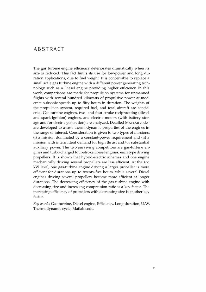
A B S T R A C TThe gas turbine engine efficiency deteriorates dramatically when itssize is reduced. This fact limits its use for low-power and long du-ration applications, due to fuel weight. It is conceivable to replace asmall scale gas turbine engine with a different power generating tech-nology such as a Diesel engine providing higher efficiency. In thiswork, comparisons are made for propulsion systems for unmannedflights with several hundred kilowatts of propulsive power at mod-erate subsonic speeds up to fifty hours in duration. The weights ofthe propulsion system, required fuel, and total aircraft are consid-ered. Gas-turbine engines, two- and four-stroke reciprocating (dieseland spark-ignition) engines, and electric motors (with battery stor-age and/or electric generation) are analyzed. Detailed Matlab codesare developed to assess thermodynamic properties of the engines inthe range of interest. Consideration is given to two types of missions:(i) a mission dominated by a constant-power requirement and (ii) amission with intermittent demand for high thrust and/or substantialauxiliary power. The two surviving competitors are gas-turbine en-gines and turbo-charged four-stroke Diesel engines, each type drivingpropellers. It is shown that hybrid-electric schemes and one enginemechanically driving several propellers are less efficient. At the 500
kW level, one gas-turbine engine driving a larger propeller is moreefficient for durations up to twenty-five hours, while several Dieselengines driving several propellers become more efficient at longerdurations. The decreasing efficiency of the gas-turbine engine withdecreasing size and increasing compression ratio is a key factor. Theincreasing efficiency of propellers with decreasing size is another keyfactor.
Key words: Gas-turbine, Diesel engine, Efficiency, Long-duration, UAV,Thermodynamic cycle, Matlab code.
v
E S T R AT TOL’efficienza di un motore turbogas diminuisce sensibilmente quandosi riducono le sue dimensioni. Questo fatto limita il suo utilizzo inapplicazioni dove basse potenze e lunghe durate sono necessarie,a causa dell’elevato peso del combustibile. È quindi lecito pensaredi sostituire un piccolo motore turbogas con una diversa tecnologia,come per esempio un più efficiente motore Diesel. In questo lavorosono stati effettuati confronti tra sistemi propulsivi adatti a voli a pi-lotaggio remoto dove sono richieste alcune centinaia di kilowatt dipotenza propulsiva a velocità subsoniche fino a cinquanta ore di volo.Si è tenuto conto del peso del sistema propulsivo, del combustibilenecessario e del velivolo completo. Sono stati analizzati motori tur-bogas, motori a combustione interna due e quattro tempi (Diesel ead accensione comandata), e motori elettrici (con batterie e/o gene-ratori elettrici). Sono stati sviluppati dettagliati codici Matlab per ilcalcolo delle proprietà termodinamiche dei motori nei range di in-teresse. Si è data enfasi a due tipi di missioni: (i) una in cui è richi-esta potenza costante e (ii) una con necessità intermittente di elevataspinta e/o potenza ausiliaria a bordo. I due candidati finali sono imotori turbogas e i motori Diesel quattro tempi turbo-aspirati, cias-cuno azionante una o più eliche. Si dimostra che configurazioni i-bride e disposizioni in cui un motore è collegato meccanicamentea più eliche sono scelte poco efficienti. Per potenze intorno ai 500
kW, un motore turbogas che azioni un’elica di grandi dimensioni èla scelta più efficiente per durate fino a venticinque ore, mentre unsistema comprendente più motori Diesel azionanti un’elica ciascunodiventa più conveniente per durate maggiori. Uno dei fattori chiaveè il progressivo calo di efficienza dei motori turbogas al diminuiredelle dimensioni e all’aumentare del rapporto di compressione. Unaltro elemento fondamentale è l’aumento dell’efficienza propulsivadelle eliche al diminuire del diametro.
Parole chiave: Turbina a gas, Motore Diesel, Efficienza, Durata di volo,Drone, Ciclo termodinamico, codice Matlab.

P U B L I C AT I O N SThis thesis work has been adapted into a paper according to AIAAstandards1 and submitted for publication to the Journal of Propulsionand Power (AIAA), on November 16, 2016.
At the present date, the document is still under review.
March 20, 2017
1 See http://arc.aiaa.org/page/styleandformat for formatting details.
vii


We are like dwarfs sitting on the shoulders of giants.We see more, and things that are more distant, than they did,
not because our sight is superior or because we are taller than they,but because they raise us up, and by their great stature add to ours.
— John of Salisbury, Metalogicon (1159)
A C K N O W L E D G E M E N T SI would first like to thank my thesis advisors, prof. William A. Sirigna-no and prof. Feng Liu of the School of Mechanical and Aerospace En-gineering at University of California, Irvine. The door to their officeswas always open whenever I ran into a trouble spot or had a questionabout my research or writing. They consistently allowed this paperto be my own work, but steered me in the right direction wheneverthey thought I needed it.
My gratitude also goes to prof. Filippo Maggi of the Department ofAerospace Science and Technology at Politecnico di Milano. Despitethe distance, he always kept my research under his supervision. Hisinsightful comments and encouragement were extremely important.
The authors were encouraged by the original suggestion from Dr.Kenneth M. Rosen (General Aero-Science Consultants, LLC) that theDiesel engine could compete with the gas-turbine engine at lowerpower levels. Valuable insights about the application of reciprocatingengines were provided by Mr. Roy Primus (GE Global Research) andMr. Patrick Pierz (Insitu, Inc.). Remarkable work was done on turbineengines by Aaron M. Frisch. Without their passionate participationand input, this thesis could not have been successfully conducted.
I must express my very profound gratitude to my family for pro-viding me with unfailing support and continuous encouragementthroughout my years of study. This accomplishment would not havebeen possible without them. Finally, I would like to thank all myfriends from California, Japan, Hawaii, Belgium, El Salvador, Ger-many, Pakistan, Brazil, Iran, Mexico, Spain and Italy, which mademy journey a worth-living experience. I will never forget you.
Thank you.
Daniele Cirigliano
March 20, 2017
ix

C O N T E N T Si creation of the models 1
1 introduction 3
1.1 On Power and Weight . . . . . . . . . . . . . . . . . . . 3
1.2 Background . . . . . . . . . . . . . . . . . . . . . . . . . 4
1.3 Motivation and Objectives . . . . . . . . . . . . . . . . . 5
1.3.1 Presentation Plan . . . . . . . . . . . . . . . . . . 6
2 engines review 9
2.1 Power and Weight . . . . . . . . . . . . . . . . . . . . . . 9
2.1.1 Weight and Size . . . . . . . . . . . . . . . . . . . 13
2.2 Aircraft Configurations . . . . . . . . . . . . . . . . . . . 14
2.3 Final Remarks . . . . . . . . . . . . . . . . . . . . . . . . 16
3 thermodynamic cycle analysis 19
3.1 4-Stroke Spark Ignition Engine . . . . . . . . . . . . . . 19
3.1.1 Ideal Cycle . . . . . . . . . . . . . . . . . . . . . . 20
3.1.2 Real Cycle . . . . . . . . . . . . . . . . . . . . . . 21
3.2 4-Stroke Compression Ignition (Diesel) Engine . . . . . 32
3.2.1 Ideal Cycle . . . . . . . . . . . . . . . . . . . . . . 32
3.2.2 Real Cycle . . . . . . . . . . . . . . . . . . . . . . 33
3.3 2-Stroke Spark Ignition Engine . . . . . . . . . . . . . . 38
3.4 2-Stroke Compression Ignition (Diesel) Engine . . . . . 40
3.5 Considerations on the Models . . . . . . . . . . . . . . . 41
3.5.1 Improvements of the models . . . . . . . . . . . 42
3.6 Gas Turbine Engine . . . . . . . . . . . . . . . . . . . . . 43ii results 49
4 engines comparison 51
4.1 Application of the Models . . . . . . . . . . . . . . . . . 51
4.1.1 Optimization Process . . . . . . . . . . . . . . . . 51
4.1.2 Numerical Simulations Results . . . . . . . . . . 52
4.2 Layout Selection . . . . . . . . . . . . . . . . . . . . . . . 55
4.2.1 Altitude Compensation and Flammability Limits 57
4.3 Constant Thrust Profile . . . . . . . . . . . . . . . . . . . 59
4.4 Variable Thrust Profile . . . . . . . . . . . . . . . . . . . 59
4.5 Comparison of Proposed Mission Profiles . . . . . . . . 62
xi
xii contents5 propeller analysis 65
5.1 Momentum Theory . . . . . . . . . . . . . . . . . . . . . 65
5.2 Momentum - Blade Element Approximated Theory . . 66
5.3 Propeller Efficiency Evaluation . . . . . . . . . . . . . . 68
5.3.1 Propeller Selection . . . . . . . . . . . . . . . . . 70
5.4 Preliminary Design of the Aircraft . . . . . . . . . . . . 71
6 real engine-propeller assembly 75
6.1 New Engine-Propeller Configurations . . . . . . . . . . 75
6.2 Refining the computations . . . . . . . . . . . . . . . . . 76
6.2.1 Constant Cruise Mission . . . . . . . . . . . . . . 76
6.2.2 Variable Power Mission . . . . . . . . . . . . . . 78
6.3 Results . . . . . . . . . . . . . . . . . . . . . . . . . . . . 80
6.4 Cost Considerations . . . . . . . . . . . . . . . . . . . . 82
7 conclusions and future work 87
7.1 Conslusions . . . . . . . . . . . . . . . . . . . . . . . . . 87
7.2 Suggestions for Future Work . . . . . . . . . . . . . . . 88iii appendix 89
a engines review 91
b variable power profile 99
b.1 Take-off phase . . . . . . . . . . . . . . . . . . . . . . . . 99
b.2 Auxiliary Power Phase . . . . . . . . . . . . . . . . . . . 100
c validation of the matlab models 103
c.1 4-stroke Turbocharged Diesel Engine . . . . . . . . . . . 103
c.2 4-stroke Turbocharged Spark-Ignition Engine . . . . . . 103
c.3 2-Stroke Turbocharged Spark-Ignition Engine . . . . . . 105
c.4 2-Stroke Turbocharged Compression-Ignition Engine . 108
L I S T O F F I G U R E SFigure 1 Weight and power of the power sources inves-
tigated. . . . . . . . . . . . . . . . . . . . . . . . 10
Figure 2 Focus on weight and power of the existing re-ciprocating engines. . . . . . . . . . . . . . . . . 11
Figure 3 Focus on weight and thrust of the existing turbine-based engines. . . . . . . . . . . . . . . . . . . . 12
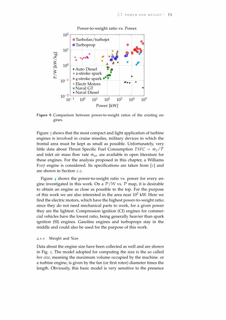
Figure 4 Comparison between power-to-weight ratios ofthe existing engines. . . . . . . . . . . . . . . . 13
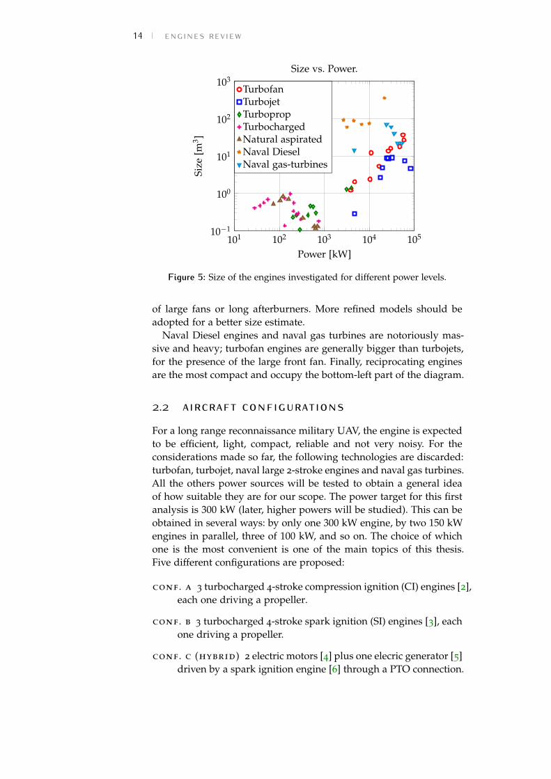
Figure 5 Size of the engines investigated for differentpower levels. . . . . . . . . . . . . . . . . . . . . 14
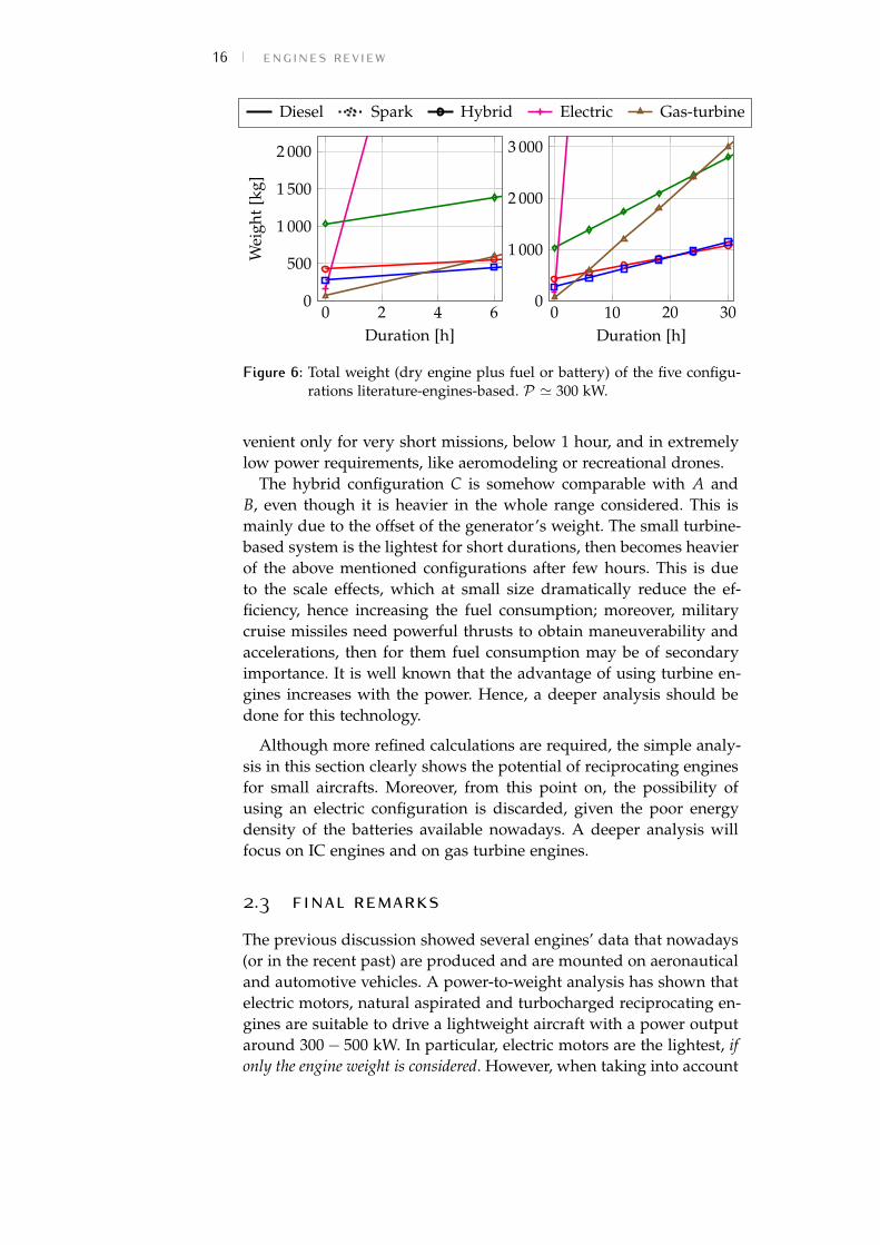
Figure 6 Total weight of the five configurations literature-engines-based. . . . . . . . . . . . . . . . . . . . 16
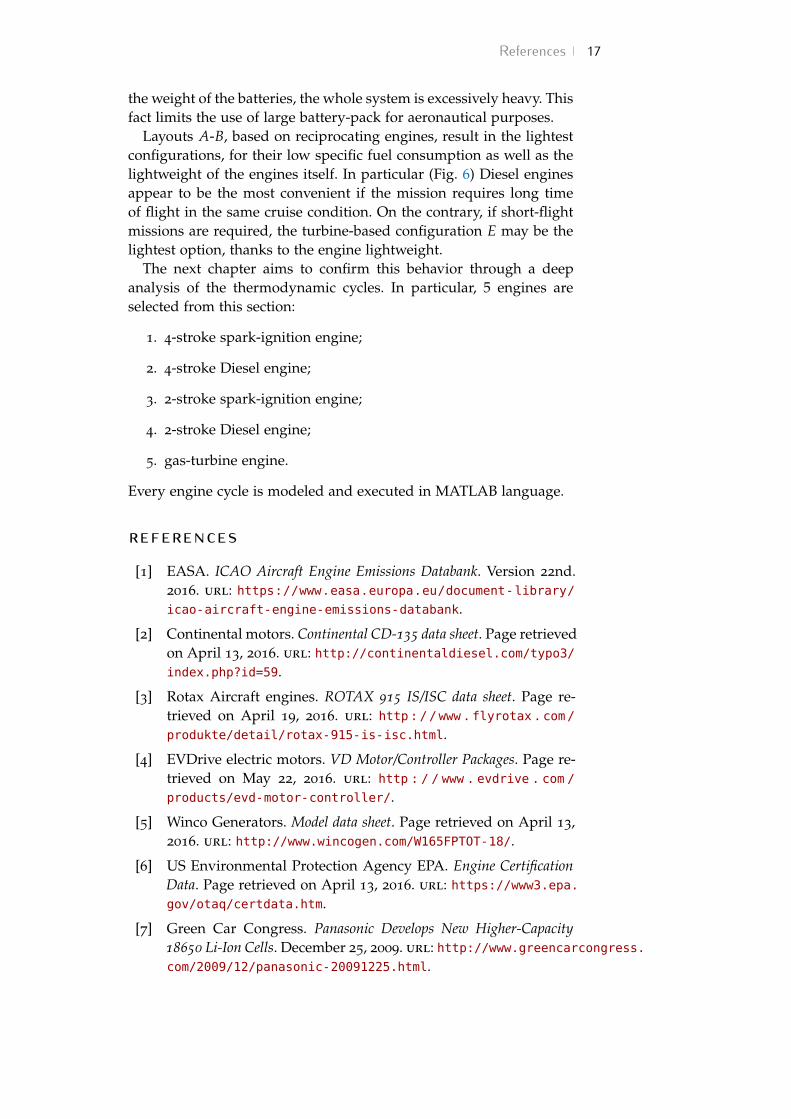
Figure 7 Volume-pressure diagram of an ideal 4-stroketurbocharged spark ignition engine. . . . . . . 20
Figure 8 Real spark-ignition cycle. . . . . . . . . . . . . . 22
Figure 9 Two zone model, cylinder schematic. . . . . . . 23
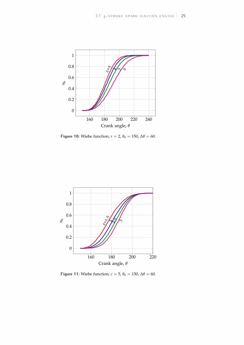
Figure 10 Wiebe function. . . . . . . . . . . . . . . . . . . 25
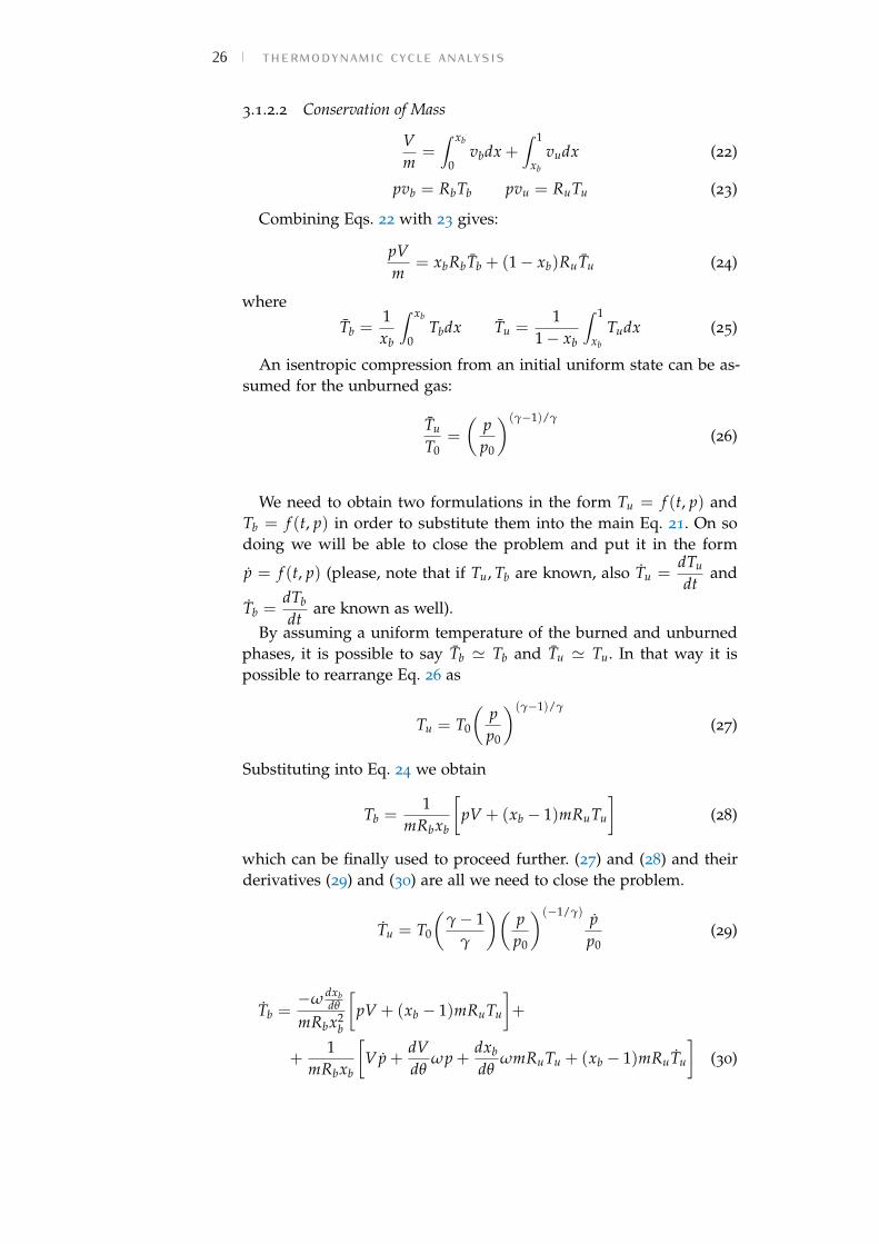
Figure 11 Wiebe function. . . . . . . . . . . . . . . . . . . 25
Figure 12 Representation of a cylinder valve. . . . . . . . 29
Figure 13 Discharge coefficient versus valve lift-over-diameterratio. . . . . . . . . . . . . . . . . . . . . . . . . 30
Figure 14 Volume-pressure diagram of an ideal 4-stroketurbocharged compression ignition engine. . . 33
Figure 15 Single zone model, cylinder schematic. . . . . 34
Figure 16 Fuel injection and heat release profile. . . . . . 37
Figure 17 2-stroke engine cylinder. . . . . . . . . . . . . . 39
Figure 18 Temperature - specific entropy real Brayton cycle. 43
Figure 19 Optimization process. . . . . . . . . . . . . . . . 53
Figure 20 Thermal efficiency of the five engines modeledby the Matlab codes. . . . . . . . . . . . . . . . 54
Figure 21 Four-stroke Diesel engine efficiency as func-tion of flight altitude. . . . . . . . . . . . . . . . 54
Figure 22 Gas-turbine engine efficiency as function of flightaltitude; OPR=40. . . . . . . . . . . . . . . . . . 54
Figure 23 Configurations considered for the analysis. . . 56
Figure 24 Comparison between configurations, constantthrust. . . . . . . . . . . . . . . . . . . . . . . . . 60
Figure 25 Power demand profile during a 50 hours mission. 62
xiii
xiv List of FiguresFigure 26 Diesel-based and turbine-based comparisons,
variable thrust. . . . . . . . . . . . . . . . . . . . 63
Figure 27 Propeller efficiency for different blade lengthand rpm. Mach: 0.3. . . . . . . . . . . . . . . . . 69
Figure 28 CT as a function of CL and CP. . . . . . . . . . 71
Figure 29 Propeller efficiency as a function of J and CP. . 72
Figure 30 Iterative process required to find the enginepower. . . . . . . . . . . . . . . . . . . . . . . . . 77
Figure 31 Iterative process required to find the enginepower. . . . . . . . . . . . . . . . . . . . . . . . . 79
Figure 32 Power requirement profile for 50 hours mission. 80
Figure 33 Comparison between different configurations;constant cruise mission. . . . . . . . . . . . . . 82
Figure 34 Comparison between different configurations;variable power mission. . . . . . . . . . . . . . 83
Figure 35 Shaft Power vs. rpm for the 4-stroke CI modeland the Thielert Centurion 2.0. . . . . . . . . . 104
Figure 36 Thermal efficiency and fuel consumption forthe 4-stroke CI model. . . . . . . . . . . . . . . 104
Figure 37 Shaft Power vs. rpm for the 4-stroke SI modeland the Rotax 914. . . . . . . . . . . . . . . . . . 105
Figure 38 Thermal Efficiency and Fuel Consumption forthe 4-stroke SI model and the Rotax 914. . . . . 106
Figure 39 Shaft Power vs. rpm for the 2-stroke SI modeland the Hirth 3003. . . . . . . . . . . . . . . . . 107
Figure 40 Fuel Consumption vs. rpm for the 2-stroke SImodel and the Hirth 3003. . . . . . . . . . . . . 107
Figure 41 Thermal Efficiency vs. rpm for the 2-stroke SImodel and the Hirth 3003. . . . . . . . . . . . . 108
L I S T O F TA B L E STable 1 Engines and power sources investigated. . . . 6
Table 2 Coefficients of the power-weight fitting curves. 9
Table 3 Specifications of the literature engines used inthe preliminary analysis. . . . . . . . . . . . . . 15
Table 4 Parameters chosen for the reciprocating enginesmodels. . . . . . . . . . . . . . . . . . . . . . . . 41
Table 5 Input parameters of the gas turbine numericalcode. . . . . . . . . . . . . . . . . . . . . . . . . 43
Table 6 Weight and efficiency of the mechanical de-vices involved in the configurations. . . . . . . 56
Table 7 Efficiency and fuel consumption of the enginesfor different altitudes. . . . . . . . . . . . . . . . 59
Table 8 Blade geometry assumptions. . . . . . . . . . . 68
Table 9 Real propeller geometry assumptions. . . . . . 71
Table 10 Performance data of the updated configurations. 81
Table 11 Performance data of the propellers selected. . 81
Table 12 Difference in weight between the Diesel andthe turbine configurations. . . . . . . . . . . . . 83
Table 13 Price of a full load of fuel for a 50 hours mission. 84
Table 14 Price of the propellers involved in the configu-rations. . . . . . . . . . . . . . . . . . . . . . . . 84
Table 15 Turbofan and Turbojet specifications. . . . . . . 93
Table 16 Cruise missiles specifications. . . . . . . . . . . 93
Table 17 Turboprop engines specifications. . . . . . . . . 95
Table 18 Electric motors specifications. . . . . . . . . . . 95
Table 19 Turbocharged engines specifications. . . . . . . 96
Table 20 Naturally aspirated engines specifications. . . 97
Table 21 Gas turbines engines specifications. . . . . . . 98
Table 22 Electric generators specifications. . . . . . . . . 98
Table 23 Thielert AG Centurion 2.0 specifications. . . . 103
Table 24 Rotax 914UL specifications. . . . . . . . . . . . 105
Table 25 Hirth 3003 100 hp specifications. . . . . . . . . 106
xv
N O M E N C L AT U R E
CD Average drag coefficient
Sp Average piston speed
minj Fuel flow through the in-jector
R Average Boltzmann con-stant of cylinder content
A Cylinder wall surface
a Acceleration at take-off
AC Curtain area
AE Effective flow area
AT Throat area
Ainj Injector cross sectionalarea
Awet Wetted wing area
B Cylinder bore
b Aircraft wing span
c Reference chord length
CD Discharge coefficient
CL Lift coefficient
CP Power coefficient
CT Thrust coefficient
cpb Specific heat pressure-constant of burned gas
CPi Induced power coefficient
cvb Specific heat volume-constant of burned gas
cvu Specific heat volume-constant of unburned gas
D Propeller diameter
Dv Valve diameter
F Net accelerating force attake-off
h Heat transfer coefficient
hi,j Sensible energy per unitmass flow
J Advance ratio
k Wall thermal conductivity
L Cylinder stroke
L/D Lift over drag ratio
Lv Valve lift
M Mach number
m Cylinder content mass
Mb Molecular mass of theburned gas
mb Burned zone mass
mc Chamber mass
m f Fuel mass
m f Mass of fuel
Mu Molecular mass of the un-burned gas
mu Unburned zone mass
mair Air mass
mcc Crankcase mass
min Mass entering the system
mout Mass leaving the system
MTIP Tip Mach number
N Engine rpm
List of Tables xviin Propeller rpm
nr Shaft revolutions per en-gine firing
pc Chamber pressure
pi Pressure at point i
pT Pressure upstream the tur-bocharger turbine
pamb Ambient pressure
pcc Crankcase pressure
Pr Prandtl number
Q Heat energy
Qb Fuel low heating value
Qch Energy released by com-bustion
Qht Energy lost by heat trans-fer to the walls
Qin Energy entering the sys-tem
Qout Energy leaving the system
Qsens Sensible energy
r/R Radial coordinate over ra-dius
Rb Boltzmann constant ofburned gas
Ru Boltzmann constant of un-burned gas
S Entropy
T Cylinder content tempera-ture
Tb Temperature of burnedzone
Tc Chamber temperature
Ti Temperature at point i
Tm Mean temperature
Tu Temperature of unburnedzone
Tw Cylinder walls tempera-ture
Tamb Ambient temperature
Tcc Crankcase temperature
U Internal energy
V Cylinder content volume
Vb Burned zone volume
vb Specific volume of burnedgas
Vc Chamber volume
Vc Clearance volume
Vi Volume at point i
Vu Unburned zone volume
vu Specific volume of un-burned gas
Vcc Crankcase volume
W Work energy
w Induced velocity
xb Mass fraction burned
z Altitude
Greek Letters
α Air–fuel ratio
αst Stoichiometric air–fuel ra-tio
ηb Combustion efficiency
ηc Compressor adiabatic effi-ciency
ηd Diffuser adiabatic effi-ciency
ηm Mechanical efficiency
xviii List of Tablesηconv Energy conversion effi-
ciency
ηel Electric motor efficiency
ηgear Gearbox efficiency
ηid Ideal efficiency
ηmech Mechanical efficiency
ηprop Propeller efficiency
ηth Thermal efficiency
γ Specific heat ratio
γb Specific heat ratio ofburned zone
γc Specific heat ratio of com-pression stroke
γe Specific heat ratio of ex-pansion stroke
µ Dynamic viscosity
ω Rotational speed
Φ Equivalence ratio
φ Flow coefficient
πb Combustion chamberpressure ratio
πc Turbocharger compres-sion ratio
πd Diffuser pressure ratio
πt Turbine pressure ratio
Ψ Stage loading coefficient
ρ Density
σ Blade solidity
τc Compressor temperatureratio
τt Turbine temperature ratio
Θ Cycle temperature ratio
θ Crank angle
ε Cylinder compression ra-tio
Other Symbols
A Propeller disc area
B Propeller blade number
L Propeller blade length
P Power
Pc Compressor power
Pi Induced power
Ps Net shaft power
Pt Turbine power
Pu Useful power
Pcruise Engine power at cruise
Pprop Propeller input power
R Degree of reaction
T Thrust
Tcruise Aircraft thrust at cruise
TTO Aircraft thrust at take-off
V True airspeed
Vjet Exhaust gases velocity
VTO Aircraft speed at take-off
W Weight
W0 Take-off gross weight
Wcrew Crew weight
We Empty structural weight
W f uel Fuel weight
Wpayload Payload weight

A C R O N Y M SAF Activity Factor
BDC Bottom Dead Center
CA Crank Angle
CFD Computational Fluid Dynamics
CI Compression Ignition
EM Electric Motor
GB Gearbox
KE Kinetic Energy
LEAP Leading Edge Aviation Propulsion
LHV Low Heating Value
OPR Overall Pressure Ratio
PTO Power Take Off
SI Spark Ignition
ST Specific Thrust
TBO Time Between Overhaul
TBR Time Between Replacement
TDC Top Dead Center
TSFC Thrust Specific Fuel Consumption
UAV Unmanned Aerial Vehicle
WAR Wetted Aspect Ratio
xix


Part I
C R E AT I O N O F T H E M O D E L S

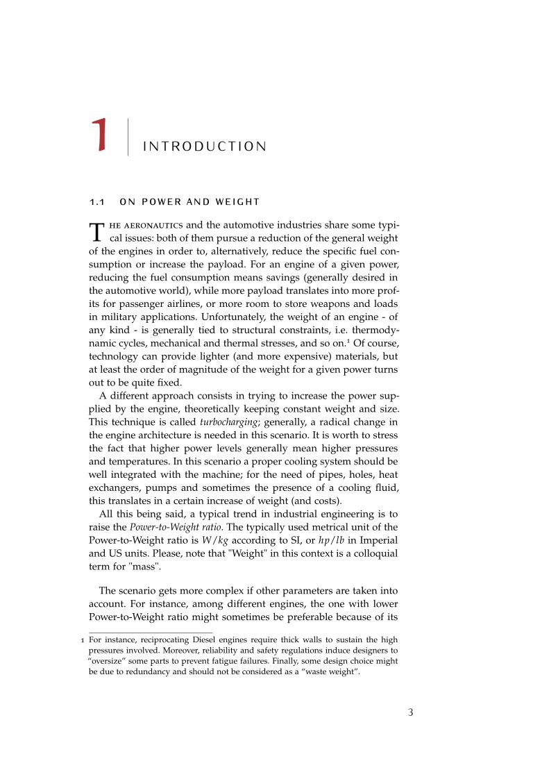
1 I N T R O D U C T I O N1.1 on power and weightT he aeronautics and the automotive industries share some typi-
cal issues: both of them pursue a reduction of the general weightof the engines in order to, alternatively, reduce the specific fuel con-sumption or increase the payload. For an engine of a given power,reducing the fuel consumption means savings (generally desired inthe automotive world), while more payload translates into more prof-its for passenger airlines, or more room to store weapons and loadsin military applications. Unfortunately, the weight of an engine - ofany kind - is generally tied to structural constraints, i.e. thermody-namic cycles, mechanical and thermal stresses, and so on.1 Of course,technology can provide lighter (and more expensive) materials, butat least the order of magnitude of the weight for a given power turnsout to be quite fixed.
A different approach consists in trying to increase the power sup-plied by the engine, theoretically keeping constant weight and size.This technique is called turbocharging; generally, a radical change inthe engine architecture is needed in this scenario. It is worth to stressthe fact that higher power levels generally mean higher pressuresand temperatures. In this scenario a proper cooling system should bewell integrated with the machine; for the need of pipes, holes, heatexchangers, pumps and sometimes the presence of a cooling fluid,this translates in a certain increase of weight (and costs).
All this being said, a typical trend in industrial engineering is to Since typical valuesof Power-to-Weightrange from 102 to104 W/kg, oftenkW/kg is preferred.
raise the Power-to-Weight ratio. The typically used metrical unit of thePower-to-Weight ratio is W/kg according to SI, or hp/lb in Imperialand US units. Please, note that "Weight" in this context is a colloquialterm for "mass".
The scenario gets more complex if other parameters are taken intoaccount. For instance, among different engines, the one with lowerPower-to-Weight ratio might sometimes be preferable because of its
1 For instance, reciprocating Diesel engines require thick walls to sustain the highpressures involved. Moreover, reliability and safety regulations induce designers to“oversize” some parts to prevent fatigue failures. Finally, some design choice mightbe due to redundancy and should not be considered as a “waste weight”.
3
4 introductionhigher thermal efficiency. In a general sense, the efficiency of a thermalengine relates the useful work with the energy available to perform it.Hence, one may want to maximize the first aspect (increase the out-put work/power) or minimize the second (decrease the fuel mass/-mass flow rate), depending on the mission profile. This type of ana-lysis is essential for industries to be able to make informed decisionson the most efficient way to power their machines. A power-weight-efficiency analysis is the basis of this thesis.
1.2 backgroundIt is well known that scaling down gas-turbine engines results in de-creased efficiency because of the so-called scale effects: profile losses,endwall losses, Reynolds number effects, heat transfer and tip clear-ance losses. A brief explanation follows.
Scaling down the engine implies the reduction of the core size. Re-ducing the passage area, a lower mass flow rate is ingested by theengine, translating in a lower net power delivered by the machine.Moreover, due to manufacturing tolerances, the physical gap betweenthe blades and the casing is basically constant, i.e. is independent onthe engine’s size; however, the blade heights scale with the engine.It follows that the relative tip clearance increases when the enginescales down, producing a strong efficiency drop. Decreasing the sizeof the core engine past an inlet diameter of 10 cm, results in effi-ciencies approaching 80% and below. The reduced efficiency is alsothe result of another source of loss: the low Reynolds number. TheReynolds number effects occur from an increase of viscous dissipa-tion loss from boundary layers. The lower the Reynolds number, thelarger the boundary layers and therefore more viscous dissipationand energy lost from the flow.
The master thesis of Aaron Frisch [1] finds that, at very low size andpower (inlet diameter below 10 cm and 300 kW), the gas-turbine en-gine efficiency becomes too low. It is conceivable that at some point itcan be replaced by another source of power, such as an internal com-bustion (IC) engine. The Diesel cycle is theoretically more efficientthan the Otto cycle, given the higher compression ratios and lean-burn combustion. Hence, a Diesel engine may be the best candidatefor this purpose, resulting in the same amount of power generationyet at a higher efficiency.
UAVs (Unmanned Aerial Vehicles) are often used in long militarymissions, like reconnaissance flights. Current technology allows theseplanes to fly at altitudes up to 25000 feet, but engineers are designingreconnaissance UAVs able to fly up to 50000 feet in the near future[2]. One of the most critical requirements is the time a reconnaissanceUAV can fly continuously without refueling. Because UAVs are notburdened with the physiological limitations of human pilots, they
1.3 motivation and objectives 5can be designed for maximized on-station times. The maximum flightduration of unmanned aerial vehicles varies widely, depending on thepower source. Solar electric UAVs, for example, hold the potential forunlimited flight, a concept championed by the Helios Prototype [3]and accomplished by the Solar Impulse Project in 2016, the first solosolar flight circumnavigation of the globe. On the other hand, the full-solar propulsion is suitable only for those applications where highthrust and large payloads are not required.
Several studies aim to find alternative UAV power sources. For in-stance, [4] explains the potential of using laser power to extend UAV’sflight duration. A clear example is the Stalker UAS, produced byLockheed Martin, which can carry a payload of 2 lbs for a maximumof 2 hours (extended to 5.5 lbs and 8 hours in the XE version) [5]. Bythe use of a photovoltaic receiver and on-board power managementhardware, the vehicle can be powered for over 48 hours.
For 40 hours missions and beyond, the fuel cell can be the bestcandidate if thrust and payload are not negligible, or for the produc-tion of electrical power on-board. Current technology is exploring theuse of solid hydrogen rods instead of gaseous hydrogen in fuel cells;while the use of rods is suitable for 2-20 kW power plants, the exces-sive weight of large 100 kW cells may be justified only if very longmissions are involved [6].
For mid-long mission durations, between 20 and 40 hours, the re-ciprocating engine is likely the best candidate to drive the aircraft, be-cause of its higher efficiency (i.e. lower fuel consumption) comparedto a turbine engine of the same power [7].
1.3 motivation and objectivesThere exist pressures from policy-makers to move towards a com-mon fuel which would be of the type used for jet or diesel engines.Thus, we are left with questions concerning the optimal selection ofengine type and configuration for long-duration, lower-to-mid sub-sonic speed of lighter aircraft. Which engine type is optimal for agiven duration? How many engines should be used for a given enginetype to produce a certain required thrust? Might an hybrid electric-combustion power source be helpful? Can one engine power morethan one propeller either by direct mechanical connection or electri-cal generation for electric motors? Is there a threshold flight durationwhen replacing the gas turbine engine with another power source re-sults in less fuel needed? These are examples of the questions to beaddressed here. A 300− 500 kW is considered as the power target inthis work.
Although some practical knowledge is already part of the "know-how" of aircraft industries, as far as author knowledge no hints of athorough and analytical selection guideline supported by solid theo-
6 introductionTable 1: Engines and power sources investigated.
Turbine engines Turbofan
Turbojet
Turboprop
Cruise missiles
Gas turbines for naval applications
Electric motors All types
Reciprocating engines Diesel and spark ignition
2- and 4-strokes
Turbocharged and naturally aspirated
retical basis is available in the literature. This work aims to answer theprevious questions by means of selection criteria based on efficiencyand weight.
1.3.1 Presentation PlanAt first, a review on the engines available nowadays is performed inChapter 2. The propulsive technologies investigated are summarizedin Table 1. Considerations on power, weight and size are outlined. Bymultiplying the fuel consumption by the flight duration, the weight ofthe fuel needed to accomplish that mission is obtained. Hence, boththe dry weight and the full weight2 are studied in this work. On so do-ing, the flight duration is the parameter used to compare the variousengines’ full weight. A deeper analysis on different engines configura-tions3 developing ' 500 kW is made. The application of each enginetechnology in Table 1 to different mission durations is investigated.
Taken the results of Chapter 2, the most promising engines from Ta-ble 1 -those ones requiring the lowest full weight per mission- are selected,discarding the others. On these candidates, an analysis of the thermo-dynamic cycle is performed in Chapter 3: a numerical Matlab codeis developed for each one of them. These engines are compared fordifferent levels of power, altitude and mission duration.
2 The dry weight is basically the weight of all the mechanical parts of the engine,including manifolds, cooling systems and casing. The full weight is the sum ofthe dry weight plus the fuel weight. The amount of fuel needed for a certain mis-sion, in terms of mass, is given by (fuel consumption [kg/s])× (mission duration [s]).For a more intuitive reading of the fuel consumption, from now on [liters/hour]will be used, and the mass of fuel will be given by (fuel density [kg/lt]) ×(fuel consumption [lt/h])× (mission duration [h]).
3 Configuration: assembly of a certain number of engines, propellers, power devicesand mechanical joints mounted on an aircraft.
References 7In the second part, a further selection is made and just few can-
didates are deeply analyzed in Chapter 4. Four configurations areinvestigated for propelling a long range reconnaissance drone, vary-ing the number of engines and propellers. However, the influence ofthe propeller number, size, rpm and aerodynamics can clearly play arole in the choice. For this reason Chapter 5 focuses on the propellerefficiency evaluation. Finally, Chapter 6 shows the application of thecoupled engine-propeller assembly, based on the analyses previouslymade. It will be shown that for a certain power requirement, thereis a best choice on which engine to use, depending on cruise missionduration and altitude.
references[1] A. M. Frisch. “Scaling Effects on the Performance and Efficiency
of Gas Turbine Engines.” Master of Science Project. Universityof California, Irvine, 2014.
[2] M. Peck. “U.S. Air Force seeks ideas for de-icing Reapers.” In:Aerospace America 54.3 (2016), p. 5.
[3] The UAVs. A brief introduction to the UAV Endurance. May 22,2016. url: http://www.theuav.com/.
[4] S. Frink. Alternative UAV power sources becoming a reality. 11
September 2012. Military & Aerospace Electronics. url: http://www.militaryaerospace.com/articles/2012/09/alternative-
uav-power.html.
[5] Lockheed Martin. Stalker UAS. Retrieved October 20, 2016. 2016.url: http://www.lockheedmartin.com/us/products/stalker-uas.html.
[6] K. Button. “Powering Airlines with hydrogen.” In: AerospaceAmerica 54.2 (2016), p. 5.
[7] N. E. Daidzic, L. Piancastelli, and A. Cattini. “Diesel engines forlight-to-medium helicopters and airplanes (Editorial).” In: Inter-national Journal of Aviation, Aeronautics, and Aerospace 1.3 (2014).url: http://commons.erau.edu/ijaaa/vol1/iss3/2.

2 E N G I N E S R E V I E W2.1 power and weightI n this study, many engine types have been investigated. Data on
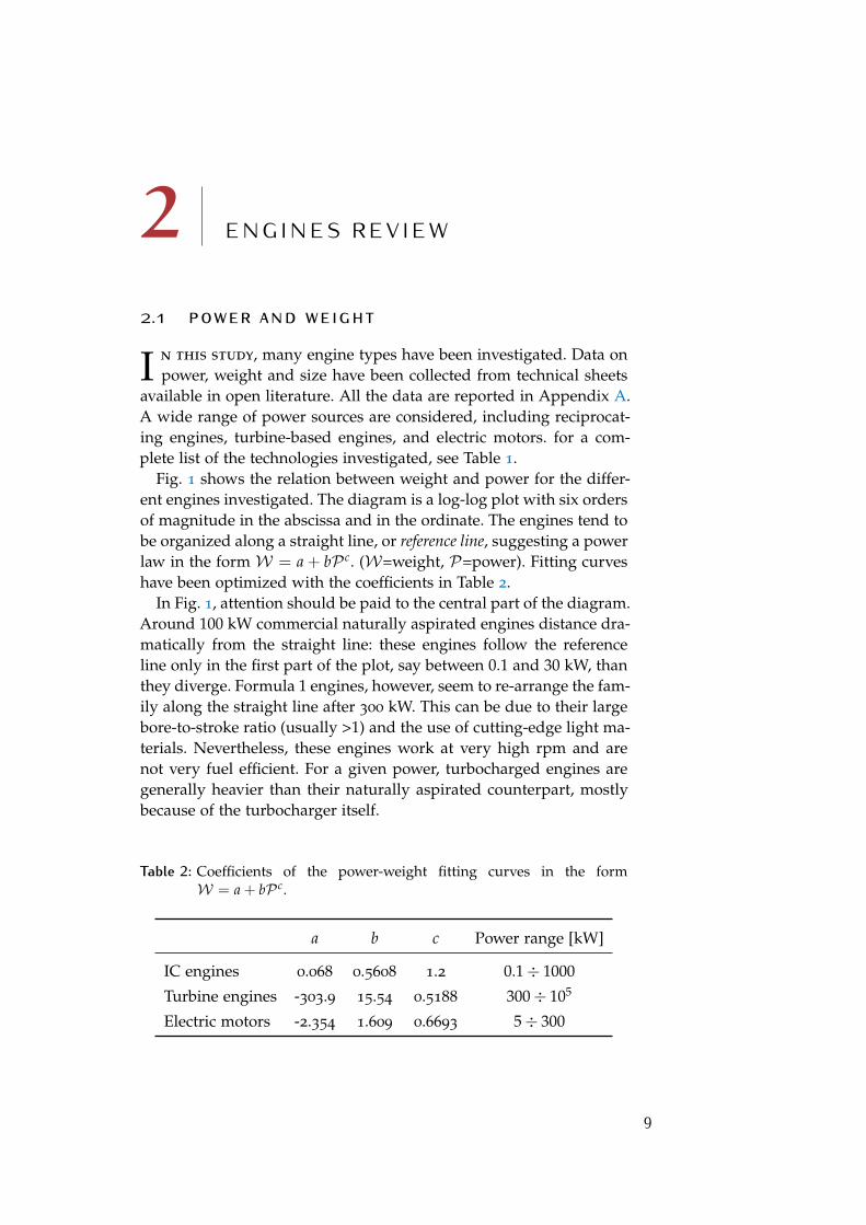
power, weight and size have been collected from technical sheetsavailable in open literature. All the data are reported in Appendix A.A wide range of power sources are considered, including reciprocat-ing engines, turbine-based engines, and electric motors. for a com-plete list of the technologies investigated, see Table 1.
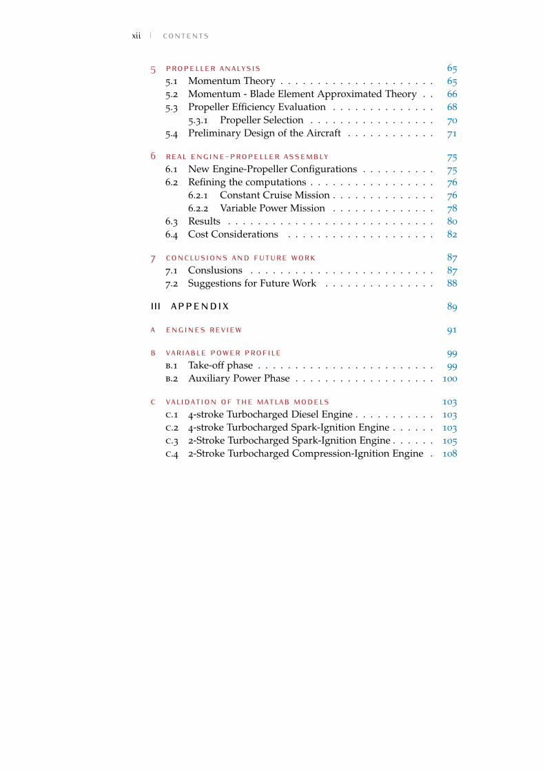
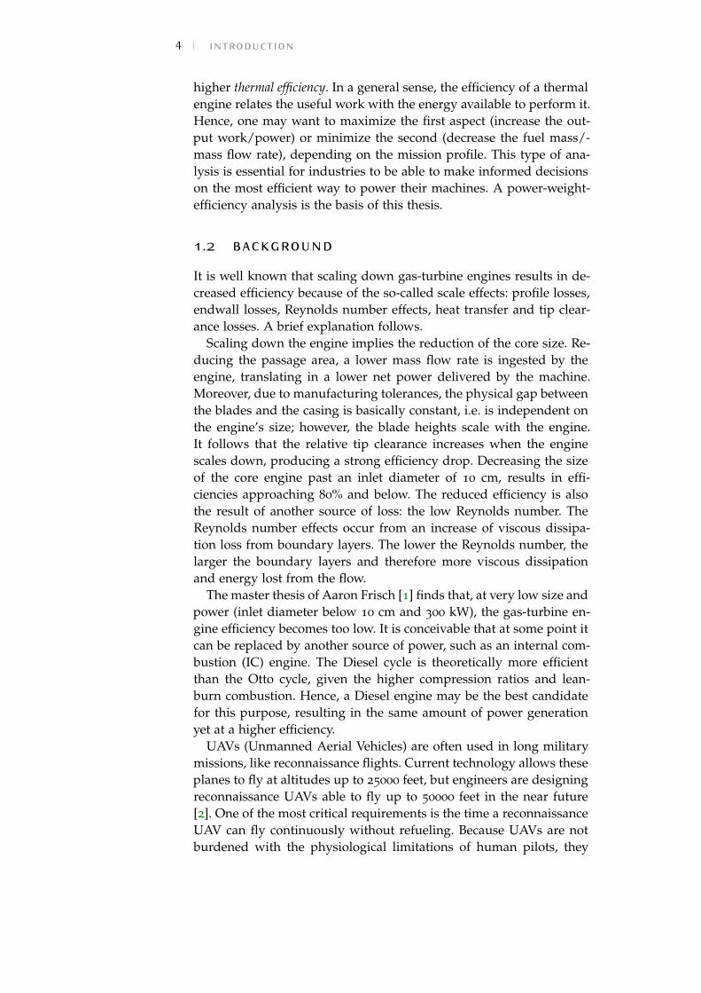
Fig. 1 shows the relation between weight and power for the differ-ent engines investigated. The diagram is a log-log plot with six ordersof magnitude in the abscissa and in the ordinate. The engines tend tobe organized along a straight line, or reference line, suggesting a powerlaw in the form W = a + bP c. (W=weight, P=power). Fitting curveshave been optimized with the coefficients in Table 2.
In Fig. 1, attention should be paid to the central part of the diagram.Around 100 kW commercial naturally aspirated engines distance dra-matically from the straight line: these engines follow the referenceline only in the first part of the plot, say between 0.1 and 30 kW, thanthey diverge. Formula 1 engines, however, seem to re-arrange the fam-ily along the straight line after 300 kW. This can be due to their largebore-to-stroke ratio (usually >1) and the use of cutting-edge light ma-terials. Nevertheless, these engines work at very high rpm and arenot very fuel efficient. For a given power, turbocharged engines aregenerally heavier than their naturally aspirated counterpart, mostlybecause of the turbocharger itself.
Table 2: Coefficients of the power-weight fitting curves in the formW = a + bP c.
a b c Power range [kW]
IC engines 0.068 0.5608 1.2 0.1÷ 1000
Turbine engines -303.9 15.54 0.5188 300÷ 105
Electric motors -2.354 1.609 0.6693 5÷ 300
9
10 engines review
10−1 100 101 102 103 104 10510−2
10−1
100
101
102
103
104
IC
Turbine
EM
Weight [kg]
Pow
er[k
W]
Weight vs. Power
TurbochargedNaturally aspiratedTurbopropTurbofanTurbojetElectric Motors
Figure 1: Weight and power of the power sources investigated.
Turbocharged engines range between 20 and 1000 kW. For a givenpower output, two opposite trends take place in these engines: onone side the additional weight of the turbocharger make them heav-ier than their naturally aspirated counterpart; on the other side, dueto the larger amount of compressed air in the pistons and in the man-ifolds, they can be smaller (but also thicker to sustain the higher pres-sure). The first trend, however, is predominant, and they are almostalways the heaviest between turbocharged and naturally aspiratedengines, for a fixed power. The weights of turbocharged engines varylittle over a wide power range. These engines are one order of magni-tude heavier than what the average reference line would suggest.
Turboprop engines follow the straight line, but due to the architec-ture of the engine itself, they seem to be used only for applicationsover 100 kW. Turbofan and turbojet engines occupy the top-right partof the diagram. Both the categories are lower limited by 103 kW, andreach easily 105 kW when high by-pass turbofan and afterburningjet engines are involved. For the same power, however, turbojet en-gines are lighter; turbofan engines suffer from the additional weightof the outer bypass channel and the large fan. Cruise missiles are themost compact and light application among turbine engines; they fitthe same linear trend (on a log− log plot) of larger turbine-based en-gines. The use of one of these power sources on an aircraft could fitthe purpose of this work; unfortunately, most of the data concerningthese engines, like weight, power and fuel consumption, are confiden-tial. The electric motors investigated are located on the reference lineand can be manufactured in a large range of power: below 1 kW, e.g.for aircraft modeling, up to tens of kW.
2.1 power and weight 11
10−1 100 101 102 103 104 105
10−1
101
103
105
107
Power [kW]
Wei
ght
[kg]
Weight vs. Power
2-strokes Diesel4-strokes Diesel2-strokes Spark4-strokes SparkNaval IC Diesel
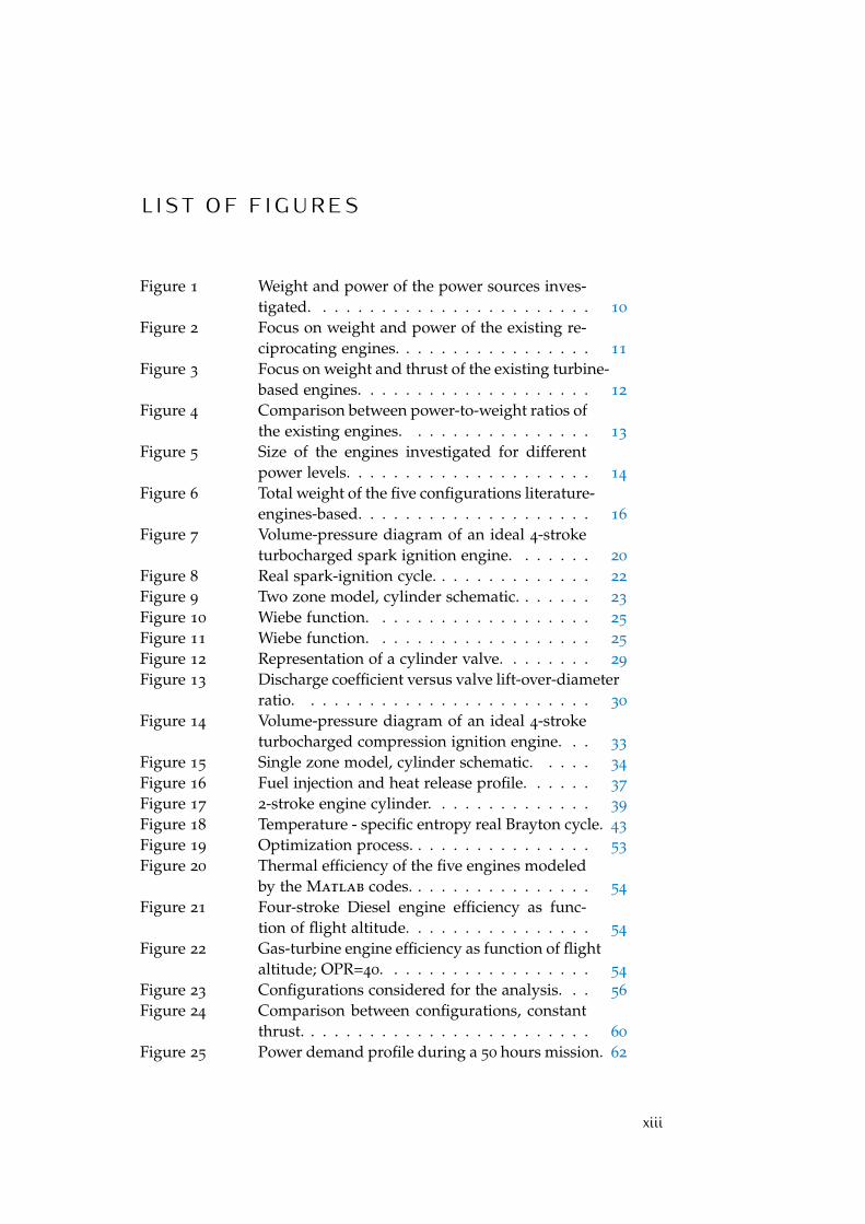
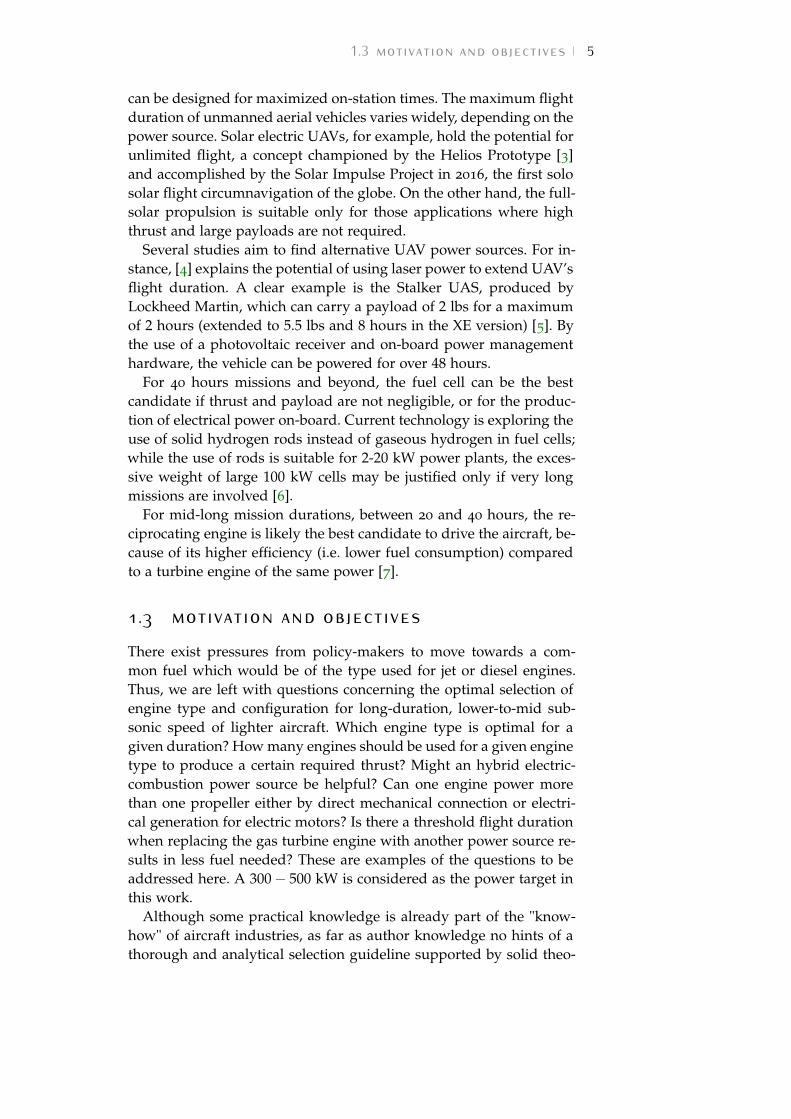
Figure 2: Focus on weight and power of the existing reciprocating engines.
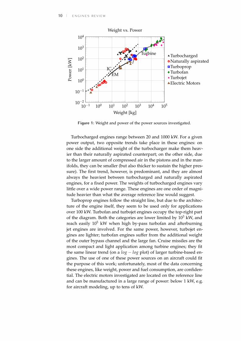
From the previous discussion, turbofan and turbojet engines arediscarded for the purpose of this work, both for their weight andbecause they largely exceed the power range of interest, 300 kW. Be-cause of their lightness, electric motors might seem to be the mostsuitable for this mission. Reciprocating engines are available too, butattention should be paid to the engine architecture to determine theactual weight.
Figure 2 shows the reciprocating engines weight versus power indetail, focusing on the ignition technique. In the region of 102 kW,specifications of 2 and 4-stroke Diesel engines and also 4-stroke sparkignition engines are available. 2-stroke spark ignition engines aremostly used in small displacement motorcycles, hence their poweroutput is limited to few horse power, say 15 hp (12 kW). In fact, 4-stroke spark-ignition engines are generally preferable for more pow-erful motorbikes.
Naval 2 strokes Diesel engines, instead, are extremely massive andheavy, and are reported here just for comparison. This family of en-gines is characterized by very low bore-to-stroke ratios (below 0.1)and rpm usually between 30 and 100. It is obvious that they are notsuited for aeronautic purposes, because of the size, weight and power.
Finally, it can be noted that in the range between 100 and 300 kW,SI engines are lighter than CI engines. This is due to a general lighterarchitecture of the former, which don’t need to withstand the highcylinder pressures typical of Diesel engines. Moreover, SI engines usu-ally have more slender cylinders, allowing them to reach very highrpm.
12 engines review
103 104 105 106101
102
103
104
Thrust [N]
Wei
ght
[kg]
Weight vs. Thrust
TurbofanTurbojetCruise missiles
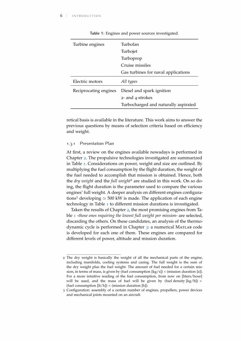
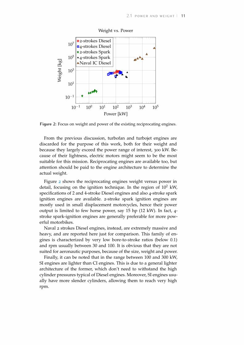
Figure 3: Focus on weight and thrust of the existing turbine-based engines.
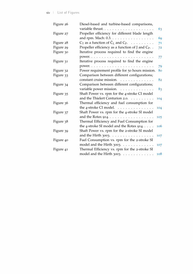
In Fig. 3 a detail of turbine engines is presented. These engines aregenerally reported according to their thrust instead of power. Hence,for comparing this family with the other engines of Table 1, a con-version from thrust to power is needed. As a first computation, for asteady level flight, neglecting the lower order ram thrust:
Vjet =T
(mair + m f )
P =12
[(mair + m f )V2
jet
] (1)
It follows that, in order to know the power of a turbine-based engine,the static thrust, the inlet air mass flow rate and the fuel mass flowrate must be known. If the thrust is given at a certain flight speed,ram thrust must be taken into account too.
To take into account the fuel needed for a given mission, the rateof fuel burning must be known. There exist two main definitions offuel consumption:
thrust specific fuel consumption TSFC =mf
T is a measureof how much fuel is injected to produce a certain amount ofthrust. It is generally used in aeronautical turbine engines andis measured in kg/N·s or lb/N·s.
brake specific fuel consumption BSFC =mf
P measures the amountof fuel burned to supply a certain power output. It is typicallyused for comparing the efficiency of internal combustion en-gines with a shaft output. Its units are kg/W·s or lb/hp·s.
2.1 power and weight 13
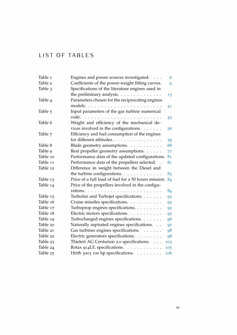
10−1 100 101 102 103 104 10510−2
10−1
100
101
102
Turbofan/turbojetTurboprop
Auto Diesel2-stroke spark4-stroke sparkElectr MotorsNaval GTNaval Diesel
Power [kW]
P/W
[kW
/kg]
Power-to-weight ratio vs. Power.
Figure 4: Comparison between power-to-weight ratios of the existing en-gines.
Figure 3 shows that the most compact and light application of turbineengines is involved in cruise missiles, military devices in which thefrontal area must be kept as small as possible. Unfortunately, verylittle data about Thrust Specific Fuel Consumption TSFC = m f /Tand inlet air mass flow rate mair are available in open literature forthese engines. For the analysis proposed in this chapter, a WilliamsF107 engine is considered. Its specifications are taken from [1] andare shown in Section 2.2.
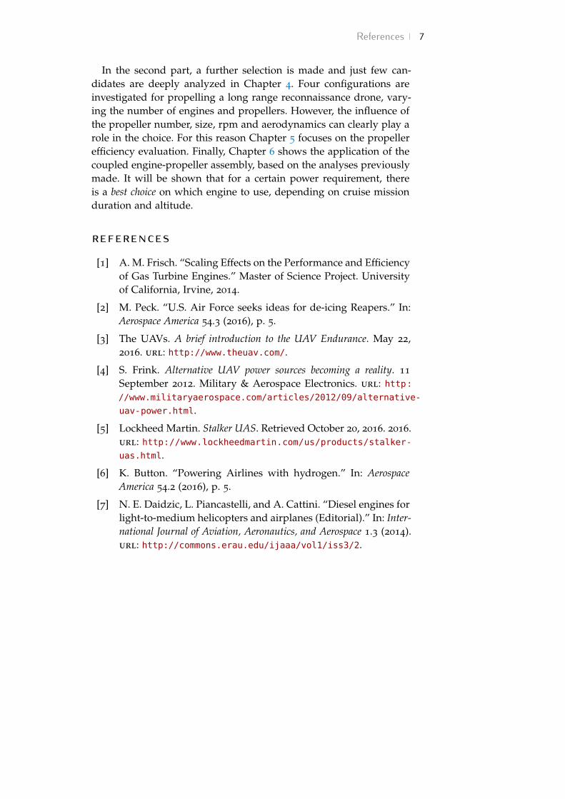
Figure 4 shows the power-to-weight ratio vs. power for every en-gine investigated in this work. On a P/W vs. P map, it is desirableto obtain an engine as close as possible to the top. For the purposeof this work we are also interested in the area near 102 kW. Here wefind the electric motors, which have the highest power-to-weight ratio:since they do not need mechanical parts to work, for a given powerthey are the lightest. Compression ignition (CI) engines for commer-cial vehicles have the lowest ratio, being generally heavier than sparkignition (SI) engines. Gasoline engines and turboprops stay in themiddle and could also be used for the purpose of this work.
2.1.1 Weight and SizeData about the engine size have been collected as well and are shownin Fig. 5. The model adopted for computing the size is the so calledbox size, meaning the maximum volume occupied by the machine. ora turbine engine, is given by the fan (or first rotor) diameter times thelength. Obviously, this basic model is very sensitive to the presence
14 engines review
101 102 103 104 10510−1
100
101
102
103
Power [kW]
Size
[m3 ]
Size vs. Power.
TurbofanTurbojetTurbopropTurbochargedNatural aspiratedNaval DieselNaval gas-turbines
Figure 5: Size of the engines investigated for different power levels.
of large fans or long afterburners. More refined models should beadopted for a better size estimate.
Naval Diesel engines and naval gas turbines are notoriously mas-sive and heavy; turbofan engines are generally bigger than turbojets,for the presence of the large front fan. Finally, reciprocating enginesare the most compact and occupy the bottom-left part of the diagram.
2.2 aircraft configurationsFor a long range reconnaissance military UAV, the engine is expectedto be efficient, light, compact, reliable and not very noisy. For theconsiderations made so far, the following technologies are discarded:turbofan, turbojet, naval large 2-stroke engines and naval gas turbines.All the others power sources will be tested to obtain a general ideaof how suitable they are for our scope. The power target for this firstanalysis is 300 kW (later, higher powers will be studied). This can beobtained in several ways: by only one 300 kW engine, by two 150 kWengines in parallel, three of 100 kW, and so on. The choice of whichone is the most convenient is one of the main topics of this thesis.Five different configurations are proposed:
conf . a 3 turbocharged 4-stroke compression ignition (CI) engines [2],each one driving a propeller.
conf . b 3 turbocharged 4-stroke spark ignition (SI) engines [3], eachone driving a propeller.
conf . c (hybrid) 2 electric motors [4] plus one elecric generator [5]driven by a spark ignition engine [6] through a PTO connection.
2.2 aircraft configurations 15Table 3: Specifications of the literature engines used in the preliminary
analysis.
Config. Engine name Weight [kg] Fuel cons. [kg/h]
A Centurion/Thielert 135 134 21.43
B ROTAX 915 IS/ISC 84 29.00
C 5.2 V10 FSI 220 58.97
D EVD150/260+HVRcr 45.8 1379
E Tomahawk F107 66 238.10
conf . d 3 electric motors taking energy from a battery pack carriedon-board [7].
conf . e One single small gas turbine engine [1], driving a propellerby means of a gearbox.
Data concerning the literature engines involved in each configura-tion are reported in Table 3. In this analysis, a standard 76 kg pro-peller is considered [8] for each engine in configurations A-D. More-over, a standard 15 kg two stage gearbox is added to the overallweight when needed. Electric motors in the range 100-200 hp (75-150kW) generally have efficiencies between 0.94 and 0.97 [9]. Hence, inthis analysis a 0.97 efficiency (defined as the ratio between output andinput power) is assumed for each electric motor. For the engines in-stalled in the configurations above, the data on fuel consumption (e.g.TSFC) are presented in Appendix A; they are taken from [1], [10],[11], [12] for the turbine engines, from [2] and [6] for reciprocatingengines.
This preliminary analysis investigates the full aircraft weight for amission. Given the same power level, the total weight of each config-uration is given by the sum of the weights of the engines, the pro-pellers, the gearboxes plus the fuel needed for each mission. Notethat for configuration D the weight of the battery pack is consideredinstead of the fuel. A standard energy density of 0.645 MJ/kg is as-sumed, according to the current technology [7]. The results are shownin Fig. 6. The figure on the left is zoomed in the interval 0-6 hours toemphasize the short-flight zone.
While the dry weight is lower in the SI configuration, the CI enginebenefits from a lower fuel consumption - the lines approach eachother. Hence, from 20 hours on, Diesel engines are the lightest devices forpropelling a 300 kW aircraft. This can be seen in Fig. 6, on the right.On the other hand, we see that configuration D is by far the heaviest,since the weight of the batteries available nowadays is still too high.An electric aircraft carrying batteries on board turns out to be con-
16 engines review
0 2 4 60
500
1 000
1 500
2 000
Duration [h]
Wei
ght
[kg]
0 10 20 300
1 000
2 000
3 000
Duration [h]
Diesel Spark Hybrid Electric Gas-turbine
Figure 6: Total weight (dry engine plus fuel or battery) of the five configu-rations literature-engines-based. P ' 300 kW.
venient only for very short missions, below 1 hour, and in extremelylow power requirements, like aeromodeling or recreational drones.
The hybrid configuration C is somehow comparable with A andB, even though it is heavier in the whole range considered. This ismainly due to the offset of the generator’s weight. The small turbine-based system is the lightest for short durations, then becomes heavierof the above mentioned configurations after few hours. This is dueto the scale effects, which at small size dramatically reduce the ef-ficiency, hence increasing the fuel consumption; moreover, militarycruise missiles need powerful thrusts to obtain maneuverability andaccelerations, then for them fuel consumption may be of secondaryimportance. It is well known that the advantage of using turbine en-gines increases with the power. Hence, a deeper analysis should bedone for this technology.
Although more refined calculations are required, the simple analy-sis in this section clearly shows the potential of reciprocating enginesfor small aircrafts. Moreover, from this point on, the possibility ofusing an electric configuration is discarded, given the poor energydensity of the batteries available nowadays. A deeper analysis willfocus on IC engines and on gas turbine engines.
2.3 final remarksThe previous discussion showed several engines’ data that nowadays(or in the recent past) are produced and are mounted on aeronauticaland automotive vehicles. A power-to-weight analysis has shown thatelectric motors, natural aspirated and turbocharged reciprocating en-gines are suitable to drive a lightweight aircraft with a power outputaround 300− 500 kW. In particular, electric motors are the lightest, ifonly the engine weight is considered. However, when taking into account
References 17the weight of the batteries, the whole system is excessively heavy. Thisfact limits the use of large battery-pack for aeronautical purposes.
Layouts A-B, based on reciprocating engines, result in the lightestconfigurations, for their low specific fuel consumption as well as thelightweight of the engines itself. In particular (Fig. 6) Diesel enginesappear to be the most convenient if the mission requires long timeof flight in the same cruise condition. On the contrary, if short-flightmissions are required, the turbine-based configuration E may be thelightest option, thanks to the engine lightweight.
The next chapter aims to confirm this behavior through a deepanalysis of the thermodynamic cycles. In particular, 5 engines areselected from this section:
1. 4-stroke spark-ignition engine;
2. 4-stroke Diesel engine;
3. 2-stroke spark-ignition engine;
4. 2-stroke Diesel engine;
5. gas-turbine engine.
Every engine cycle is modeled and executed in MATLAB language.
references[1] EASA. ICAO Aircraft Engine Emissions Databank. Version 22nd.
2016. url: https://www.easa.europa.eu/document-library/icao-aircraft-engine-emissions-databank.
[2] Continental motors. Continental CD-135 data sheet. Page retrievedon April 13, 2016. url: http://continentaldiesel.com/typo3/index.php?id=59.
[3] Rotax Aircraft engines. ROTAX 915 IS/ISC data sheet. Page re-trieved on April 19, 2016. url: http://www.flyrotax.com/produkte/detail/rotax-915-is-isc.html.
[4] EVDrive electric motors. VD Motor/Controller Packages. Page re-trieved on May 22, 2016. url: http : / / www . evdrive . com /
products/evd-motor-controller/.
[5] Winco Generators. Model data sheet. Page retrieved on April 13,2016. url: http://www.wincogen.com/W165FPTOT-18/.
[6] US Environmental Protection Agency EPA. Engine CertificationData. Page retrieved on April 13, 2016. url: https://www3.epa.gov/otaq/certdata.htm.
[7] Green Car Congress. Panasonic Develops New Higher-Capacity18650 Li-Ion Cells. December 25, 2009. url: http://www.greencarcongress.com/2009/12/panasonic-20091225.html.
18 engines review[8] G. Gardiner. 3-D preformed composites: The leap into LEAP. Ed. by
Composites World. March 4, 2014.
[9] U.S. Energy Information Administration. Minimum efficiency stan-dards for electric motors will soon increase. September 26, 2016. To-day in Energy. url: https://www.eia.gov/todayinenergy/detail.php?id=18151.
[10] Stanford University. Data on Large Turbofan Engines. Page re-trieved on May 22, 2016. url: http : / / adg . stanford . edu /
aa241/propulsion/largefan.html.
[11] Headquarters Air Force Directorate of Propulsion. “Data forsome civil gas turbine engines.” In: The Engine Handbook. Ohio:Wright-Patterson AFB, 1991. url: http://www.aircraftenginedesign.com/TableB3.html.
[12] Jet Engine Specification Database. Military Turbojet/Turbofan Spec-ifications. March 21, 2005. url: http://www.jet-engine.net/miltfspec.html.
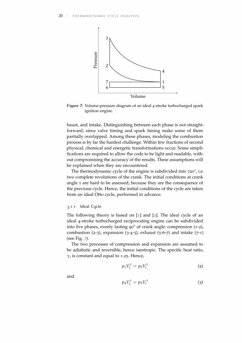
3 T H E R M O DY N A M I C C Y C L EA N A LY S I SI n order to assess the performance of a certain engine, e.g. power,
fuel consumption, efficiency, weight and geometry, two optionsare possible:
• look into the open literature and hope to find a (reliable) enginedata-sheet;
• develop a numerical code able to compute the operative prop-erties of an engine, given its geometry and some boundary con-ditions.
Although more complex, the second option allows greater flexibility,since any level of power can be theoretically assessed through thecode; nevertheless, the real feasibility of the cycle computed is notguaranteed in reality, since mechanical limits may have not been con-sidered or modeled properly. A deep research in the open literaturewas done and did not give good results, since industry is generallyreluctant to let know the performance of the engine alone; the greaterpart of the data-sheet involve the use of the engine in the vehicle andtheir performance coupled.1 These data are not useful for the presentwork.
For these reasons the numerical approach is the only way to esti-mate the engines capabilities at different operative conditions, such al-titude, aircraft speed, rpm, equivalence ratio and others. From the pre-vious section, five engines have been selected and a numerical Mat-lab code has been developed for each one of them: 4-stroke spark ig-nition, 4-stroke compression ignition, 2-stroke spark ignition, 2-strokecompression ignition, gas turbine engine. The numerical codes arebriefly discussed below.
3.1 4-stroke spark ignition engineIs well known that a 4-stroke reciprocating engine’s cycle is com-posed by five phases: compression, combustion and expansion, ex-
1 Data like the fuel consumption per kilometer are quite easy to find, but are veryvehicle-dependent and ignore several other variables in that specific configuration,like rpm, velocity, turbocharging settings, altitude (if any) etcetera.
19
20 thermodynamic cycle analysis
1
2
3
4
567
VolumePr
essu
re
Figure 7: Volume-pressure diagram of an ideal 4-stroke turbocharged sparkignition engine.
haust, and intake. Distinguishing between each phase is not straight-forward, since valve timing and spark timing make some of thempartially overlapped. Among these phases, modeling the combustionprocess is by far the hardest challenge. Within few fractions of secondphysical, chemical and energetic transformations occur. Some simpli-fications are required to allow the code to be light and readable, with-out compromising the accuracy of the results. These assumptions willbe explained when they are encountered.
The thermodynamic cycle of the engine is subdivided into 720°, i.e.two complete revolutions of the crank. The initial conditions at crankangle 1 are hard to be assessed, because they are the consequence ofthe previous cycle. Hence, the initial conditions of the cycle are takenfrom an ideal Otto cycle, performed in advance.
3.1.1 Ideal CycleThe following theory is based on [1] and [2]. The ideal cycle of anideal 4-stroke turbocharged reciprocating engine can be subdividedinto five phases, evenly lasting 90° of crank angle: compression (1-2),combustion (2-3), expansion (3-4-5), exhaust (5-6-7) and intake (7-1)(see Fig. 7).
The two processes of compression and expansion are assumed tobe adiabatic and reversible, hence isentropic. The specific heat ratio,γ, is constant and equal to 1.25. Hence,
p1Vγ1 = p2Vγ
c (2)
andp4Vγ
1 = p3Vγc (3)
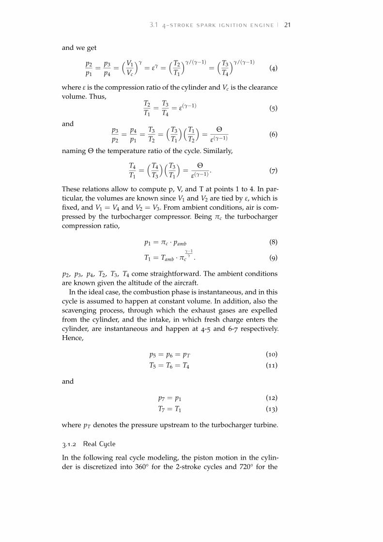
3.1 4-stroke spark ignition engine 21and we get
p2
p1=
p3
p4=(V1
Vc
)γ= εγ =
(T2
T1
)γ/(γ−1)=(T3
T4
)γ/(γ−1)(4)
where ε is the compression ratio of the cylinder and Vc is the clearancevolume. Thus,
T2
T1=
T3
T4= ε(γ−1) (5)
andp3
p2=
p4
p1=
T3
T2=(T3
T1
)(T1
T2
)=
Θε(γ−1)
(6)
naming Θ the temperature ratio of the cycle. Similarly,
T4
T1=(T4
T3
)(T3
T1
)=
Θε(γ−1)
. (7)
These relations allow to compute p, V, and T at points 1 to 4. In par-ticular, the volumes are known since V1 and V2 are tied by ε, which isfixed, and V1 = V4 and V2 = V3. From ambient conditions, air is com-pressed by the turbocharger compressor. Being πc the turbochargercompression ratio,
p1 = πc · pamb (8)
T1 = Tamb · πγ−1
γc . (9)
p2, p3, p4, T2, T3, T4 come straightforward. The ambient conditionsare known given the altitude of the aircraft.
In the ideal case, the combustion phase is instantaneous, and in thiscycle is assumed to happen at constant volume. In addition, also thescavenging process, through which the exhaust gases are expelledfrom the cylinder, and the intake, in which fresh charge enters thecylinder, are instantaneous and happen at 4-5 and 6-7 respectively.Hence,
p5 = p6 = pT (10)
T5 = T6 = T4 (11)
and
p7 = p1 (12)
T7 = T1 (13)
where pT denotes the pressure upstream to the turbocharger turbine.
3.1.2 Real CycleIn the following real cycle modeling, the piston motion in the cylin-der is discretized into 360° for the 2-stroke cycles and 720° for the
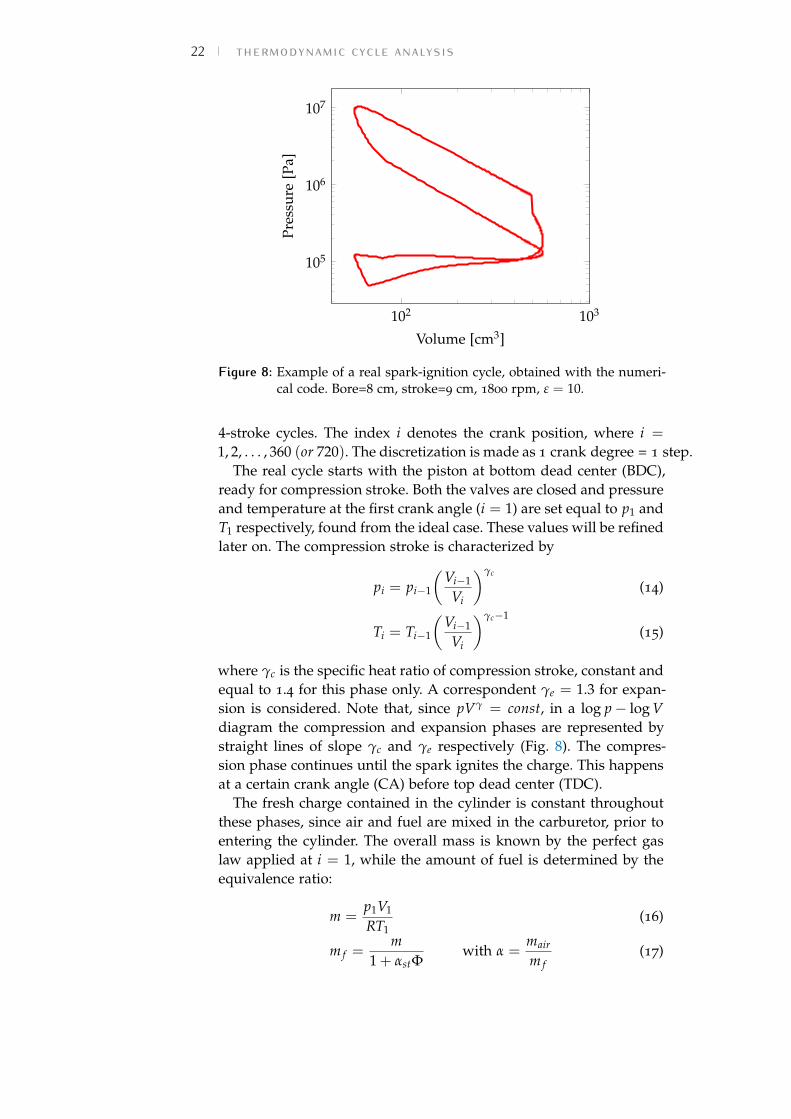
22 thermodynamic cycle analysis
102 103
105
106
107
Volume [cm3]
Pres
sure
[Pa]
Figure 8: Example of a real spark-ignition cycle, obtained with the numeri-cal code. Bore=8 cm, stroke=9 cm, 1800 rpm, ε = 10.
4-stroke cycles. The index i denotes the crank position, where i =
1, 2, . . . , 360 (or 720). The discretization is made as 1 crank degree = 1 step.The real cycle starts with the piston at bottom dead center (BDC),
ready for compression stroke. Both the valves are closed and pressureand temperature at the first crank angle (i = 1) are set equal to p1 andT1 respectively, found from the ideal case. These values will be refinedlater on. The compression stroke is characterized by
pi = pi−1
(Vi−1
Vi
)γc
(14)
Ti = Ti−1
(Vi−1
Vi
)γc−1
(15)
where γc is the specific heat ratio of compression stroke, constant andequal to 1.4 for this phase only. A correspondent γe = 1.3 for expan-sion is considered. Note that, since pVγ = const, in a log p− log Vdiagram the compression and expansion phases are represented bystraight lines of slope γc and γe respectively (Fig. 8). The compres-sion phase continues until the spark ignites the charge. This happensat a certain crank angle (CA) before top dead center (TDC).
The fresh charge contained in the cylinder is constant throughoutthese phases, since air and fuel are mixed in the carburetor, prior toentering the cylinder. The overall mass is known by the perfect gaslaw applied at i = 1, while the amount of fuel is determined by theequivalence ratio:
m =p1V1
RT1(16)
m f =m
1 + αstΦwith α =
mair
m f(17)
3.1 4-stroke spark ignition engine 23
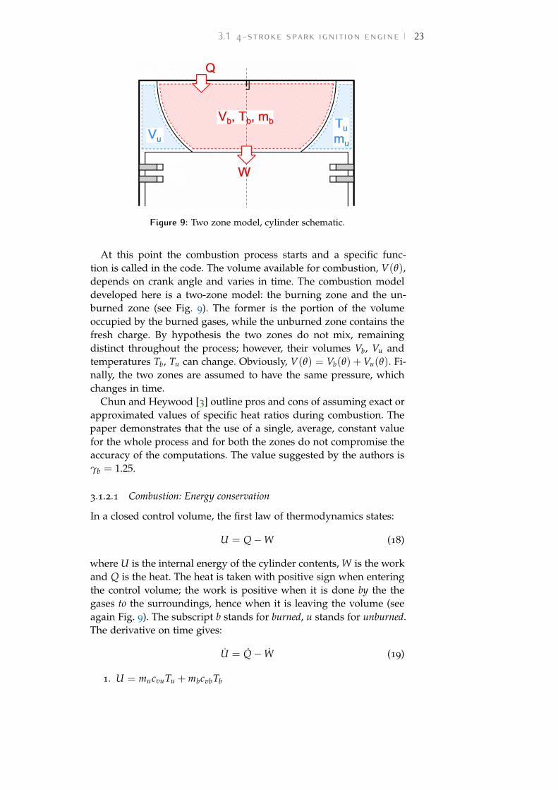
Figure 9: Two zone model, cylinder schematic.
At this point the combustion process starts and a specific func-tion is called in the code. The volume available for combustion, V(θ),depends on crank angle and varies in time. The combustion modeldeveloped here is a two-zone model: the burning zone and the un-burned zone (see Fig. 9). The former is the portion of the volumeoccupied by the burned gases, while the unburned zone contains thefresh charge. By hypothesis the two zones do not mix, remainingdistinct throughout the process; however, their volumes Vb, Vu andtemperatures Tb, Tu can change. Obviously, V(θ) = Vb(θ) + Vu(θ). Fi-nally, the two zones are assumed to have the same pressure, whichchanges in time.
Chun and Heywood [3] outline pros and cons of assuming exact orapproximated values of specific heat ratios during combustion. Thepaper demonstrates that the use of a single, average, constant valuefor the whole process and for both the zones do not compromise theaccuracy of the computations. The value suggested by the authors isγb = 1.25.
3.1.2.1 Combustion: Energy conservation
In a closed control volume, the first law of thermodynamics states:
U = Q−W (18)
where U is the internal energy of the cylinder contents, W is the workand Q is the heat. The heat is taken with positive sign when enteringthe control volume; the work is positive when it is done by the thegases to the surroundings, hence when it is leaving the volume (seeagain Fig. 9). The subscript b stands for burned, u stands for unburned.The derivative on time gives:
U = Q− W (19)
1. U = mucvuTu + mbcvbTb
24 thermodynamic cycle analysisU = mucvuTu + mucvuTu + mbcvbTb + mbcvbTb
U = m[− dxb
dθωcvuTu + (1− xb)cvuTu +
dxb
dθωcvbTb + xbcvbTb
]2. Q = Qch − Qht
1) Qch = m f LHV
Qch = m fdxb
dθωLHV
2) Qht = hA(Tb − Tw)
3. W = pdVdt
W = pωdVdθ
where ω is the rotational speed, m f is the fuel mass, xb is the massfraction burned, LHV is the fuel Low Heating Value, h is the heattransfer coefficient, Tw is the temperature of the cylinder walls, which
is assumed constant for simplicity, anddxb
dθis the burning rate with
respect to the crank angle.The mass fraction burned is given by the Wiebe function:
xb = 1− exp[− c(
θ − θ0
∆θ
)r+1 ](20)
where θ is the crank angle, θ0 is the start of combustion, ∆θ is the totalcombustion duration (xb = 0 to xb = 1), and c and r are adjustableparameters. The function is reported in Fig. 10, for variable values ofc, and in Fig. 11 for variable values of r. Varying c and r changes theshape of the curve significantly. In particular, the change of c acts asa delay in the end of the combustion, while r acts like a trigger in thevery beginning of the process. According to [1], actual mass fractioncurves have been fitted with c = 5 and r = 2.Substituting the equations above in Eq. 19 gives:
−m fdxb
dθωLHV + hA(Tb − Tw) + pω
dVdθ
+
+ m[− dxb
dθωcvuTu + (1− xb)cvuTu+
+dxb
dθωcvbTb + xbcvbTb
]= 0 (21)
i.e. a differential equation in Tb, Tu. To proceed further, models forthe thermodynamic properties of the burned and unburned gasesare required.
3.1 4-stroke spark ignition engine 25
160 180 200 220 240
0
0.2
0.4
0.6
0.8
1
c=5
4 3 2
Crank angle, θ
x b
Figure 10: Wiebe function; r = 2, θ0 = 150, ∆θ = 60.
160 180 200 220
0
0.2
0.4
0.6
0.8
1
r=1.5
2
2.5 3
Crank angle, θ
x b
Figure 11: Wiebe function; c = 5, θ0 = 150, ∆θ = 60.
26 thermodynamic cycle analysis3.1.2.2 Conservation of Mass
Vm
=∫ xb
0vbdx +
∫ 1
xb
vudx (22)
pvb = RbTb pvu = RuTu (23)
Combining Eqs. 22 with 23 gives:
pVm
= xbRbTb + (1− xb)RuTu (24)
where
Tb =1xb
∫ xb
0Tbdx Tu =
11− xb
∫ 1
xb
Tudx (25)
An isentropic compression from an initial uniform state can be as-sumed for the unburned gas:
Tu
T0=
(pp0
)(γ−1)/γ
(26)
We need to obtain two formulations in the form Tu = f (t, p) andTb = f (t, p) in order to substitute them into the main Eq. 21. On sodoing we will be able to close the problem and put it in the form
p = f (t, p) (please, note that if Tu, Tb are known, also Tu =dTu
dtand
Tb =dTb
dtare known as well).
By assuming a uniform temperature of the burned and unburnedphases, it is possible to say Tb ' Tb and Tu ' Tu. In that way it ispossible to rearrange Eq. 26 as
Tu = T0
(pp0
)(γ−1)/γ
(27)
Substituting into Eq. 24 we obtain
Tb =1
mRbxb
[pV + (xb − 1)mRuTu
](28)
which can be finally used to proceed further. (27) and (28) and theirderivatives (29) and (30) are all we need to close the problem.
Tu = T0
(γ− 1
γ
)(pp0
)(−1/γ) pp0
(29)
Tb =−ω dxb
dθ
mRbx2b
[pV + (xb − 1)mRuTu
]+
+1
mRbxb
[Vp +
dVdθ
ωp +dxb
dθωmRuTu + (xb − 1)mRuTu
](30)
3.1 4-stroke spark ignition engine 27Substituting Tb (Eq. 30) and Tu (Eq. 29) in Eq. 21, a differential equa-tion in p only is obtained. It comes in the form p = f (t, p).
For simplicity, let us define:
A1 = −m fdxb
dθωLHV (31)
A2 = hA(Tb − Tw) (32)
A3 = pωdVdθ
(33)
A4 = −mdxb
dθωcvuTu (34)
A5 = m(1− xb)cvuT0
(γ− 1
γ
)(pp0
)−1/γ
(35)
A6 = ��mdxb
dθωcvb
1��m Rbxb
[pV + (xb − 1)mRuTu
](36)
A7 = ��mZZxb cvb
{ −ω dxbdθ
��m RbxA2b
[pV + (xb − 1)mRuTu
]}(37)
A8 =��mZZxb cvb
��m RbZZxb
(dVdθ
ωp +dxb
dθωmRuTu
)(38)
Hence, we can write:
A1 + A2 + A3 + A4 + A5pp0
+ A6 + A7 + A8+
+cv,b
Rb
[Vp + (xb − 1)mRuT0
(γ− 1
γ
)(pp0
)−1/γ pp0
]= 0 (39)
Defining
A9 = A1 + A2 + A3 + A4 + A6 + A7 + A8 (40)
A10 =
[A5
p0+
cvb
RbV +
cvb
Rb(xb − 1)mRuT0
(γ− 1
γ
)(pp0
)−1/γ 1p0
](41)
we finally obtain
p = − A9
A10(42)
which is a compact way to write the ode in the form p = f (t, p).A correlation for the heat transfer h coefficient is required. In thisanalysis the Annand [4] correlation is used:(
hBk
)= a
(ρSpB
µ
)b
(43)
The value of a varies with intensity of charge motion and enginedesign. Generally, 0.35 ≤ a ≤ 0.8 with b = 0.7. Gas properties areevaluated at the cylinder-average charge temperature:
Tg =pVMmR
(44)
28 thermodynamic cycle analysisM = xb Mb + (1− xb)Mu (45)
Sp =2LN60
(46)
k =µcpb
Pr; (47)
where M is the average molecular mass of the gases contained in thecylinder, Sp is the mean piston speed, N is the engine rpm, L andB are the piston stroke and bore respectively, k is the wall thermalconductivity, Pr = 0.7 is the Prandtl number, µ is the viscosity of thecylinder contents, computed by Shuterland’s correlation
µ = µre f
(Tg
Tsuth
)1.5(Tsuth + 110.4Tg + 110.4
)(48)
where µre f = 1.716 · 10−5 kgm·s and Tsuth = 291 K. Cylinder gases then
follow a polytropic expansion until exhaust valve is opened, some de-gree before bottom dead center. When exhaust valve opens, the cylin-der pressure is above the exhaust manifold pressure and a blowdownprocess occurs. During this process, the gas which remains inside thecylinder expands polytropically.
A displacement of gas out of the cylinder follows the blowdownprocess as the piston moves from BDC to TDC. As long as a pressuredifference between the cylinder and the manifold is present, the suc-tion of the gases will be added to the scavenging process; during thisphase the cylinder volume reduces, causing a rise in pressure.
3.1.2.3 Flow Trough Valves
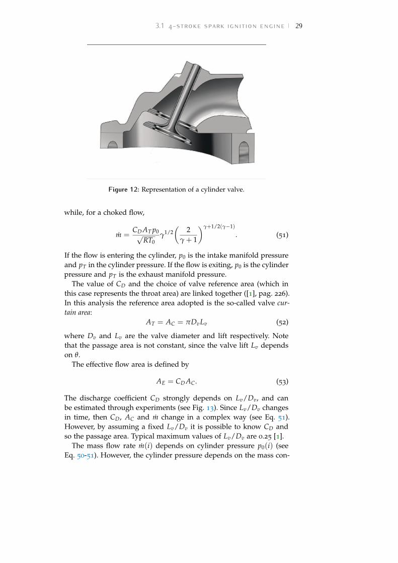
When a pressure difference is present between two points of a duct, amass flow rate from the high pressure zone towards the low pressurezone is established. The smallest cross area of the duct, if present,is called throat. In reciprocating engines this scenario is typical ofthe valves connecting the manifolds to the cylinders. The system isrepresented in Fig. 12.
For given values of p0 and T0 (the stagnation conditions), the max-imum mass flow occurs when the velocity at the throat equals thespeed of sound. This condition is called choking or critical flow. Whenthe flow is choked the pressure at the throat, pT, is related to thestagnation pressure p0 as follows:
pT
p0=
(2
γ + 1
)γ/γ−1
(49)
This ratio is called critical pressure ratio and depends on γ only. Forγ = 1.4 the critical pressure ratio is 0.528. For subcritical flow, thereal mass flow rate established in the duct is
m =CD AT p0√
RT0
(pT
p0
)1/γ{ 2γ
γ− 1
[1−
(pT
p0
)(γ−1)/γ]}1/2
. (50)
3.1 4-stroke spark ignition engine 29
Figure 12: Representation of a cylinder valve.
while, for a choked flow,
m =CD AT p0√
RT0γ1/2
(2
γ + 1
)γ+1/2(γ−1)
. (51)
If the flow is entering the cylinder, p0 is the intake manifold pressureand pT in the cylinder pressure. If the flow is exiting, p0 is the cylinderpressure and pT is the exhaust manifold pressure.
The value of CD and the choice of valve reference area (which inthis case represents the throat area) are linked together ([1], pag. 226).In this analysis the reference area adopted is the so-called valve cur-tain area:
AT = AC = πDvLv (52)
where Dv and Lv are the valve diameter and lift respectively. Notethat the passage area is not constant, since the valve lift Lv dependson θ.
The effective flow area is defined by
AE = CD AC. (53)
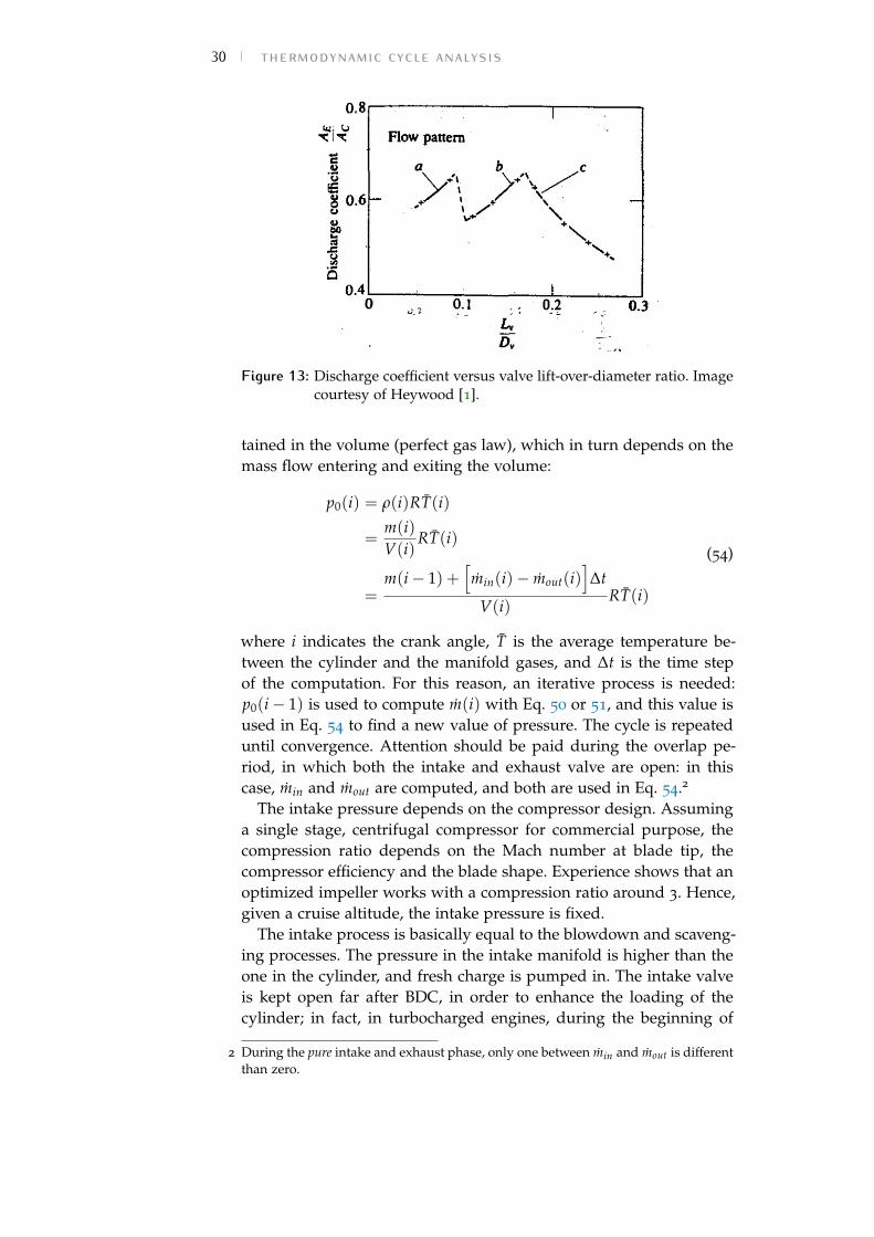
The discharge coefficient CD strongly depends on Lv/Dv, and canbe estimated through experiments (see Fig. 13). Since Lv/Dv changesin time, then CD, AC and m change in a complex way (see Eq. 51).However, by assuming a fixed Lv/Dv it is possible to know CD andso the passage area. Typical maximum values of Lv/Dv are 0.25 [1].
The mass flow rate m(i) depends on cylinder pressure p0(i) (seeEq. 50-51). However, the cylinder pressure depends on the mass con-
30 thermodynamic cycle analysis
Figure 13: Discharge coefficient versus valve lift-over-diameter ratio. Imagecourtesy of Heywood [1].
tained in the volume (perfect gas law), which in turn depends on themass flow entering and exiting the volume:
p0(i) = ρ(i)RT(i)
=m(i)V(i)
RT(i)
=m(i− 1) +
[min(i)− mout(i)
]∆t
V(i)RT(i)
(54)
where i indicates the crank angle, T is the average temperature be-tween the cylinder and the manifold gases, and ∆t is the time stepof the computation. For this reason, an iterative process is needed:p0(i− 1) is used to compute m(i) with Eq. 50 or 51, and this value isused in Eq. 54 to find a new value of pressure. The cycle is repeateduntil convergence. Attention should be paid during the overlap pe-riod, in which both the intake and exhaust valve are open: in thiscase, min and mout are computed, and both are used in Eq. 54.2
The intake pressure depends on the compressor design. Assuminga single stage, centrifugal compressor for commercial purpose, thecompression ratio depends on the Mach number at blade tip, thecompressor efficiency and the blade shape. Experience shows that anoptimized impeller works with a compression ratio around 3. Hence,given a cruise altitude, the intake pressure is fixed.
The intake process is basically equal to the blowdown and scaveng-ing processes. The pressure in the intake manifold is higher than theone in the cylinder, and fresh charge is pumped in. The intake valveis kept open far after BDC, in order to enhance the loading of thecylinder; in fact, in turbocharged engines, during the beginning of
2 During the pure intake and exhaust phase, only one between min and mout is differentthan zero.
3.1 4-stroke spark ignition engine 31compression the pressure in the cylinder is still lower than the man-ifold pressure. New charge enters the cylinder until the inlet valvecloses; we are now into a new cycle, beyond 720°.
The intake process lasts until the intake valve closes, which gener-ally happens several degrees after BC, exploiting the flow’s inertia inorder to fill the cylinder with fresh charge as much as possible. Whenthe valve closes, the cylinder state is described by a pressure, temper-ature and mass content that very unlikely will be the same as thoseat the same crank angle computed before. In particular, performingthe intake process until inlet valve closing corresponds to start froma different value of p1, T1, m. At this point, it is possible to performa new cycle, with a compression stroke starting from the new values.New properties will be computed by the combustion process whichwill affect the following phases. The convergence is reached whenthe thermodynamic properties at the end of the intake process matchthe starting ones of the previous iteration under a certain tolerance.Convergence is generally obtained in 2-3 iterations.
Although this iterative procedure is required to "close" the loop ina p-V diagram, the real behavior of a reciprocating engine is fullyunsteady and properties vary from one cycle to the other. Hence theperfect match of the properties is not strictly required.
3.1.2.4 Work and Power
Just as a remainder, the work W associated to a closed cycle is givenby the integral
W =∮
p dV (55)
that, discretized in the numerical code, is
W =∫ 720
1p dV '
720
∑i=1
pi ∆Vi =720
∑i=1
pi(Vi −Vi−1). (56)
where V0 = V720.In the four-stroke engine cycle, work is done on the piston during
the intake and the exhaust processes. The work done by the cylindergases on the piston during exhaust is
We =∫ 540
361p dV '
540
∑i=361
pi ∆Vi(< 0). (57)
The work done by the cylinder gases on the piston during intake is
Wi =∫ 720
541p dV '
720
∑i=541
pi ∆Vi(> 0). (58)
The net work to the piston over the exhaust and intake strokes, thepumping work, is
Wp = We + Wi. (59)
32 thermodynamic cycle analysisThe compression work made by the piston to the cylinder gases isgiven by
Wc =∫ 180
1p dV '
180
∑i=1
pi ∆Vi(< 0). (60)
Finally, the useful work made during the expansion phase is
Wu =∫ 360
181p dV '
360
∑i=181
pi ∆Vi(> 0). (61)
Engine’s thermal efficiency is defined as
ηth =W
m f LHV=
Pm f LHV
. (62)
The definition of W depends on authors. Some considerW = Wu + Wc, others take into account the pumping work too:W = Wu + Wc + Wp. In this analysis the second approach is adopted,as suggested by [1]. Power is defined as
P =W rpm60 nr
(63)
where nr is the number of shaft revolutions per engine firing. A four-stroke engine fires once every two revolutions (nr = 2), while a two-stroke engine fires every revolution (nr = 1). This explains why, the-oretically, a two-stroke engine delivers twice the power than a four-stroke, given the same rpm and engine geometry.
3.2 4-stroke compression ignition (diesel) en-gineThe main difference between a spark ignition (SI) engine and a com-pression ignition (CI) engine is the combustion process. In the formerthe charge is composed by a premixed mixture of air and fuel, whilein the latter only air is drawn into the cylinder and fuel is injected inanother moment. Hence, the greater difference in the numerical codeis the combustion function. Other smaller differences are also presentand are here discussed.
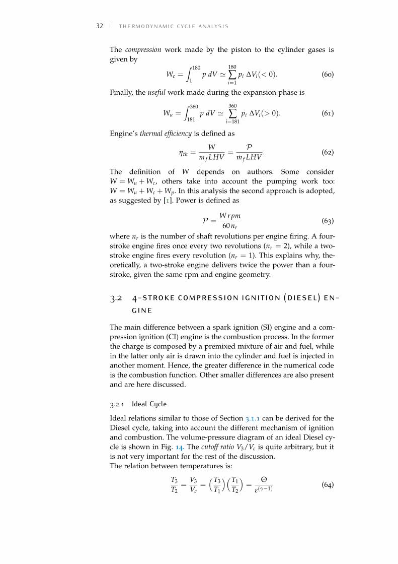
3.2.1 Ideal CycleIdeal relations similar to those of Section 3.1.1 can be derived for theDiesel cycle, taking into account the different mechanism of ignitionand combustion. The volume-pressure diagram of an ideal Diesel cy-cle is shown in Fig. 14. The cutoff ratio V3/Vc is quite arbitrary, but itis not very important for the rest of the discussion.The relation between temperatures is:
T3
T2=
V3
Vc=(T3
T1
)(T1
T2
)=
Θε(γ−1)
(64)
3.2 4-stroke compression ignition (diesel) engine 33
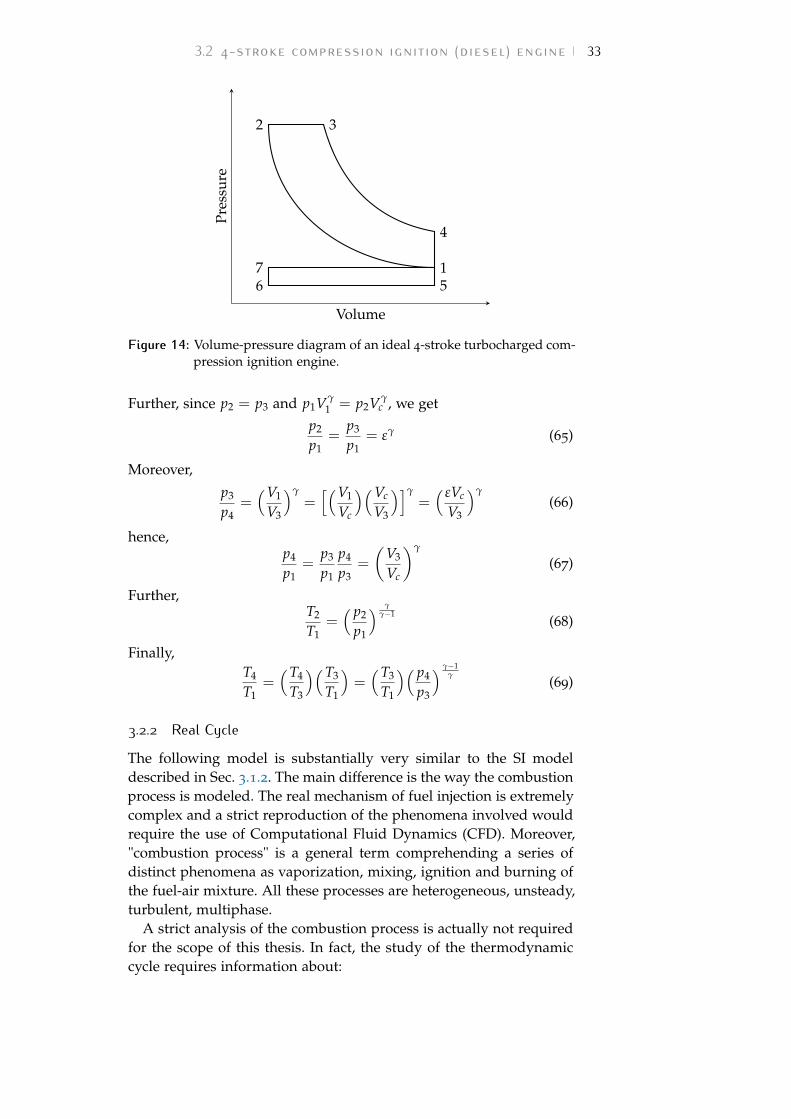
1
2 3
4
567
Volume
Pres
sure
Figure 14: Volume-pressure diagram of an ideal 4-stroke turbocharged com-pression ignition engine.
Further, since p2 = p3 and p1Vγ1 = p2Vγ
c , we getp2
p1=
p3
p1= εγ (65)
Moreover,
p3
p4=(V1
V3
)γ=[(V1
Vc
)(Vc
V3
)]γ=( εVc
V3
)γ(66)
hence,p4
p1=
p3
p1
p4
p3=
(V3
Vc
)γ
(67)
Further,T2
T1=( p2
p1
) γγ−1
(68)
Finally,T4
T1=(T4
T3
)(T3
T1
)=(T3
T1
)( p4
p3
) γ−1γ
(69)
3.2.2 Real CycleThe following model is substantially very similar to the SI modeldescribed in Sec. 3.1.2. The main difference is the way the combustionprocess is modeled. The real mechanism of fuel injection is extremelycomplex and a strict reproduction of the phenomena involved wouldrequire the use of Computational Fluid Dynamics (CFD). Moreover,"combustion process" is a general term comprehending a series ofdistinct phenomena as vaporization, mixing, ignition and burning ofthe fuel-air mixture. All these processes are heterogeneous, unsteady,turbulent, multiphase.
A strict analysis of the combustion process is actually not requiredfor the scope of this thesis. In fact, the study of the thermodynamiccycle requires information about:
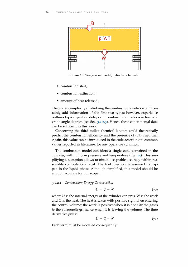
34 thermodynamic cycle analysis
Figure 15: Single zone model, cylinder schematic.
• combustion start;
• combustion extinction;
• amount of heat released.
The grater complexity of studying the combustion kinetics would cer-tainly add information of the first two types; however, experienceoutlines typical ignition delays and combustion durations in terms ofcrank angle degrees (see Sec. 3.2.2.3). Hence, these experimental datacan be sufficient in this work.
Concerning the third bullet, chemical kinetics could theoreticallypredict the combustion efficiency and the presence of unburned fuel.Again, this value can be introduced in the code according to commonvalues reported in literature, for any operative condition.
The combustion model considers a single zone contained in thecylinder, with uniform pressure and temperature (Fig. 15). This sim-plifying assumption allows to obtain acceptable accuracy within rea-sonable computational cost. The fuel injection is assumed to hap-pen in the liquid phase. Although simplified, this model should beenough accurate for our scope.
3.2.2.1 Combustion: Energy Conservation
U = Q−W (70)
where U is the internal energy of the cylinder contents, W is the workand Q is the heat. The heat is taken with positive sign when enteringthe control volume; the work is positive when it is done by the gasesto the surroundings, hence when it is leaving the volume. The timederivative gives:
U = Q− W (71)
Each term must be modeled consequently:
3.2 4-stroke compression ignition (diesel) engine 351. U = mcvT + mcvT =
Rγ− 1
(mT + mT)
2. Q = Qch − Qht + Qsens
1) Qch = mburnLHV
2) Qht = hA(T − Tw)
3) Qsens = ∑i mihi −∑j mjhj
3. W = pdVdt
= pV
where Qch is the energy released by the combustion, Qht is the heatlost to the cylinder walls, which are at constant temperature Tw, Qsens
is the sensible energy of those masses entering and leaving the vol-ume (only fuel injection is considered; crevice losses and leakagesare neglected), m is the cylinder mass at each timestep
(m(t) =
mair + m f (t)), LHV is the fuel Low Heating Value.
Assembling the terms we get the following equation:
Rγ− 1
(mT + mT) = mburnLHV − hA(T − Tw) + minjhi − pV (72)
3.2.2.2 Perfect Gas Law
At the beginning of combustion, only air is contained in the volume.By deriving in time the perfect gas equation
pV = mRT (73)
we obtainpV + pV = mRT + mRT + mRT (74)
Rearranging,
T =pV + pV − minjRT −mRT
mR(75)
where the temperature T is simply given by the perfect gas law:
T =pVmR
(76)
By substituting Eqs. 75 and 76 into Eq. 72 and rearranging:
Rγ− 1
[���minjT +
1R( pV + pV −����minjRT −mRT)
]= mburnLHV − hA(T − Tw) + minjhi − pV (77)
1R( pV + pV −mRT)
=γ− 1
R[mburnLHV − hA(T − Tw) + minjcpTf − pV
](78)
36 thermodynamic cycle analysisp =
γ− 1V
[mburnLHV − hA
(pVmR− Tw
)+ minjcpTf − pV
]− p
(VV− R
R
)(79)
Eq. 79 is a differential equation in the form p = f (t, p). V and V areknown from the cylinder geometry and rpm. The term A in the aboveequation is the area subject to heat transfer. It is given by:
A(θ) = A f ix + Avar(θ)
A f ix =
πB2
2+
4Vc
B
Avar(θ) =4(V(θ)−Vc
)πB2
(80)
The fixed term is composed by the piston crown area plus the cylin-der top wall plus the lateral cylinder walls of the clearance volume,which are always exposed to the gases. The variable term is the lat-eral surface of the cylinder that is gradually uncovered during pistonmotion.
The presence of the term R increases the overall complexity of theproblem. A possible solution is the shifting of the value of R in timebetween two typical values: 289 [J/kgK] for the exhaust gases, and273 [J/kgK] for the fresh charge. The rate of burning is modeled bythe Wiebe function (Eq. 20) [1].
R = xbR1 + (1− xb)R2 (81)
R =dRdxb
dxb
dθ
dθ
dt(82)
xb(θ) = 1− exp[− c(
θ − θ0
∆θ
)r+1](83)
dxb
dθ=
c(r + 1)∆θ
(θ − θ0
∆θ
)r
exp[− c(
θ − θ0
∆θ
)r+1](84)
R = (R1 − R2)ωc(r + 1)
∆θ
(θ − θ0
∆θ
)r
exp[− c(
θ − θ0
∆θ
)r+1](85)
In order to implement the combustion model on MATLAB ode45
solver, a characteristic shape of fuel injection minj and the fuel burningrate mburn should be defined. This is done in the following section.
3.2.2.3 Fuel Injection
The inlet fuel mass flow rate is given by the fuel flow through a noz-zle:
minj = CD Ainj
√2ρ f ∆p (86)
minj = CD Ainj
√2ρ f ∆p
∆θ
6 rpm(87)
3.2 4-stroke compression ignition (diesel) engine 37minj
0 t
˙m
start inj. end inj. end of comb.
heat
0 t
rel
60%40%
delay 1/3 2/3 end of comb.
Figure 16: Fuel injection and heat release profile according to [1].
where Ainj is the nozzle area, ρ f is the fuel density, ∆p is the pres-sure drop across the injector, CD is the discharge coefficient, and ∆θ
is the length of injection (in degrees). The CD, Ainj, ρ f and ∆θ arefixed, while minj is an input parameter. It follows that ∆p3 can beobtained by the second equation and substituted into the first. Themagnitude of fuel mass flow rate is then known. Standard Diesel in-jectors usually operate with fuel-injection pressures between 200 and1700 atmospheres ([1], pag. 522).
It is well known that the fuel injection and the heat release do nottake place simultaneously. The ignition delay in a Diesel engine is de-fined as the time (or crank angle) interval between the start of ignitionand the establishment of the flame. Heywood ([1], pg. 503) indicatesthat typical ignition delays lie between 5° and 9°. The real injectionprofile is available only from experimental data; in this analysis a stepfunction is assumed to approximate the injection rate; a heat releaseprofile is also assumed, including an ignition delay and reproducingthe heat release time distribution (Fig. 16).
The overall injection profile depends on many aspects and its shapemay vary a bit; however, the length of injection is typically around 20
crank degrees. The heat release distribution, according to [1] pag. 513,says that about 60% of the fuel burns in the first one-third of the totalcombustion period. This is the main contribute to combustion andis modeled as a rectangle of unknown height; the remaining 40% isconsumed linearly until there is fuel to sustain the combustion. Sincethe total heat released and the areas are known (60%-40%), with ele-mentary algebra it is possible to fully characterize (length and height)these shapes.
The start of injection is at 15° before TDC, and is manually movedbackwards up to 20° with increasing rpm. The most difficult data to
3 ∆p varies on time. In fact, ∆p(t) = pinj − pcyl(t).
38 thermodynamic cycle analysisbe decided is the duration of the flame. This length strictly dependson chemical kinetics, fluid dynamics and piston mechanics. For thesereasons it was decided to assume that the combustion extinguishesafter 100° from the start of injection. From that point on a simple isen-tropic expansion is considered. Another difference with the 4-strokeSI model is that the mass contained in the cylinder is not the samealong compression and expansion strokes, because of the fuel injec-tion. The equivalence ratio is computed as the ratio between the in-stantaneous air-to-fuel ratio α and the stoichiometric ratio. αst ' 14.5in Diesel engines.
3.3 2-stroke spark ignition engineThe Matlab code developed here is inspired to the work of Sookdeo[5], even if several major changes were done. The work of Sookdeoaims to model an extremely small and fast rotating CI engine, whilewe are interested in traditional dimensions and rpm; for this rea-son, the engine geometry was rearranged. Moreover, the combustionmodel present in Sookdeo’s work is oversimplified and fitted to ex-perimental data performed by himself; it was necessary to implementa new combustion model (substantially equal to those previously ex-plained) which have a general validity. Finally, a new heat transfermodel was included.
A 2-stroke engine is composed by a certain number of cylinders,in which the piston divides two very important environments. Oneis the volume contained between the piston crown and the cylinderwalls; the other one is the so-called crankcase environment, composedby the portion between the piston and the crankcase surrounding theshaft, plus a short inlet manifold from which the air is drawn into thecycle. A scheme of a two-stroke cylinder is shown in Fig. 17.
The Matlab code evaluates five thermodynamic properties for eachenvironment: cylinder pressure, mass of gases in cylinder, enthalpy,temperature and entropy. For each one of these unknowns an equa-tion is required:
pV = mRT Eq. of state
m = m0 + min −mout Mass conserv.
Q = Q0 + Qin −Qout Energy conserv.
Q = mcvT 1st Law of Therm.
Q = TdS 2nd Law of Therm.
(88)
3.3 2-stroke spark ignition engine 39
Figure 17: 2-stroke engine cylinder.
Deriving in θ, the system becomes:
dpdθ
V + pdVdθ
=dmdθ
RT + mRdTdθ
Eq. of state
dmdθ
=dmin
dθ− dmout
dθMass conserv.
dQdθ
=dQin
dθ− dQout
dθEnergy conserv.
dQdθ
=dmdθ
cvT + mcvdTdθ
1st Law of Therm.
dQdθ
=dTdθ
S + TdSdθ
2nd Law of Therm.
(89)
Remember that, for the derivation chain rule,
d·dt
=d·dθ
dθ
dt=⇒ d·
dθ=
1ω
d·dt
Equations 89 represent a system of five equations in five unknowns.Including the other set of five equations for the second environment,a 10× 10 system is obtained. Every explicit linear system can be re-arranged in matrix form: Ax = b. This problem comes in the formM(t, x)x = f (t, x). The Matlab ode45 solver is able to integrate thesystem of differential equations from t0 to t f given some initial con-ditions x0.
In this case, the problem is made by the following linear system:
Vc −RTc 0 −mcR 00 1 0 0 00 0 1 0 0 [∅]0 −cvTc 1 −mccv 00 0 1 −Sc −Tc
Vcc −RTcc 0 −mccR 00 1 0 0 0
[∅] 0 0 1 0 00 −cvTcc 1 −mcccv 00 0 1 −Scc −Tcc
ddθ
pcmcQcTcScpccmccQccTccScc
=
1ω
−ωpcdVdθ
mcc−moutQin−Qout
00
−ωpccdVdθ
min−mccQin−Qout
00
40 thermodynamic cycle analysiswith initial conditions
x0 ={
p0c m0
c 0 T0c 0 p0
cc m0cc 0 T0
cc 0}T
.
Initial pressure and temperature of the cylinder are assumed asInitial conditions
p0c = 1.4 pamb and T0
c = Tamb1.4(γ−1)/γ. Further iterations will over-write these values with the effective ones computed from the cycle.p0
cc and T0cc are set equal to the conditions in the intake manifold:
p0cc = πc pamb and T0
cc = Tambπ(γ−1)/γc . Finally, initial masses m0
c andm0
cc are computed with the perfect gas law, given the temperature andthe volume of each environment:
m0c = mair + m f
= (1 + α)mair
= (1 + αstΦ)p0
cV0c
RT0c
m0cc = (1 + αstΦ)
p0ccV0
ccRT0
cc
(90)
Note that now α is defined as the fuel-to-air ratio. The system ofdifferential equations is integrated along 360° with ODE45 solver, ob-taining the vector x at every crank angle. The Matlab solver ODE45 isbased on an explicit second order accurate Runge-Kutta method. It isa single-step solver, meaning that in computing the solution at time t,it needs only the solution at the immediately preceding time point t-1[6]. The timestep used for the four reciprocating engine models wasvaried between one crank angle up to 1/16 of crank angle. Payinga moderate increase in computational time, no significant change inthe results were noticed.
3.4 2-stroke compression ignition (diesel) en-gineThe same considerations made for adapting the 4-stroke SI model tothe 4-stroke CI model apply here. The code is substantially equal tothe 2-stroke SI code, with the main exception of a different combus-tion model (see 3.2) and other minor changes concerning the air-fuelcomposition. Note that now the inzial conditions for the mass are:
m0c = mair =
p0cV0
cRT0
c
m0cc =
p0ccV0
ccRT0
cc
(91)
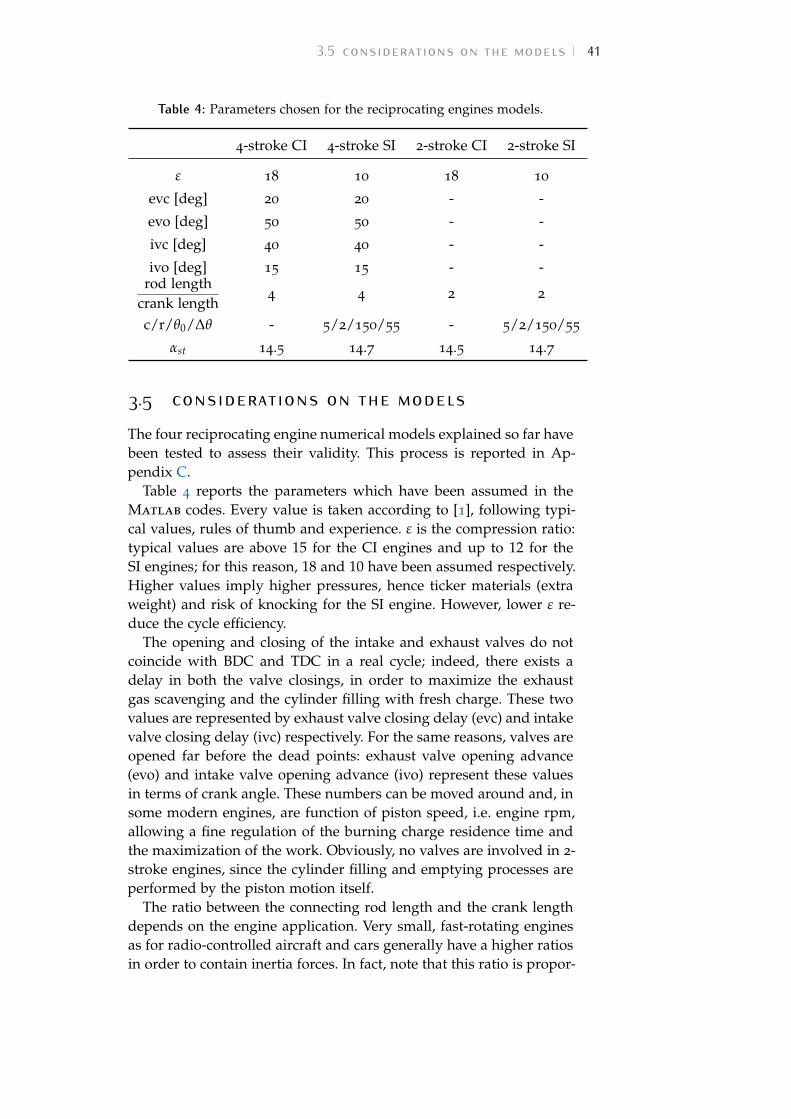
3.5 considerations on the models 41Table 4: Parameters chosen for the reciprocating engines models.
4-stroke CI 4-stroke SI 2-stroke CI 2-stroke SI
ε 18 10 18 10
evc [deg] 20 20 - -
evo [deg] 50 50 - -
ivc [deg] 40 40 - -
ivo [deg] 15 15 - -rod length
crank length4 4 2 2
c/r/θ0/∆θ - 5/2/150/55 - 5/2/150/55
αst 14.5 14.7 14.5 14.7
3.5 considerations on the modelsThe four reciprocating engine numerical models explained so far havebeen tested to assess their validity. This process is reported in Ap-pendix C.
Table 4 reports the parameters which have been assumed in theMatlab codes. Every value is taken according to [1], following typi-cal values, rules of thumb and experience. ε is the compression ratio:typical values are above 15 for the CI engines and up to 12 for theSI engines; for this reason, 18 and 10 have been assumed respectively.Higher values imply higher pressures, hence ticker materials (extraweight) and risk of knocking for the SI engine. However, lower ε re-duce the cycle efficiency.
The opening and closing of the intake and exhaust valves do notcoincide with BDC and TDC in a real cycle; indeed, there exists adelay in both the valve closings, in order to maximize the exhaustgas scavenging and the cylinder filling with fresh charge. These twovalues are represented by exhaust valve closing delay (evc) and intakevalve closing delay (ivc) respectively. For the same reasons, valves areopened far before the dead points: exhaust valve opening advance(evo) and intake valve opening advance (ivo) represent these valuesin terms of crank angle. These numbers can be moved around and, insome modern engines, are function of piston speed, i.e. engine rpm,allowing a fine regulation of the burning charge residence time andthe maximization of the work. Obviously, no valves are involved in 2-stroke engines, since the cylinder filling and emptying processes areperformed by the piston motion itself.
The ratio between the connecting rod length and the crank lengthdepends on the engine application. Very small, fast-rotating enginesas for radio-controlled aircraft and cars generally have a higher ratiosin order to contain inertia forces. In fact, note that this ratio is propor-
42 thermodynamic cycle analysistional to 1/stroke. Large naval engines typically have small rotationalspeed and bore-to-stroke ratios, hence higher strokes.
The values of c, r, θ0 and ∆θ of the Wiebe function (Eq. ??) representthe two constants of the equation, the fuel injection crank angle (i =180 corresponds to TDC) and the burning duration in terms of crankangle. Note that injection is advanced with respect to TDC; this isgenerally named spark advance and in this analysis is set to 30°. Thefaster the rotational speed, the larger should be the spark advanceallowing more time to the charge to ignite. CI engines do not workwith this combustion model, hence these parameters do not apply.
Finally, the air-to-fuel stoichiometric ratio αst is also reported in thetable. For pure octane the stoichiometric mixture is approximately14.7:1, while for Diesel fuel is around 14.5:1. Any mixture greater thanαst is considered a lean mixture; any less than αst is a rich mixture.
3.5.1 Improvements of the modelsThe accuracy of the numerical codes can be improved in several ways:
• So far, the heat loss from the burning gases to the cylinderwalls is modeled through the Annand’s correlation [4]. Refinedheat transfer models can be introduced in every combustionmodel, for example by accounting for a variable wall tempera-ture, which depends on the gases temperature. Also, radiativeheat transfer from the burning zone could be added to the con-vective one.
• Modeling the gradual opening and closing of the valves of thetwo 4-stroke engines, i.e. Lv(θ), should be done is more realis-tic results are expected; this implies that also the curtain areadepends on θ. This dependence should be included in the com-putation of the instantaneous m, Eq. 52. Further complexity isadded if the valve lift is also a function of engine’s rpm, i.e.Lv(θ, rpm).
• The 4-stroke Diesel model considers a single zone contained inthe cylinder, with uniform pressure and temperature. Compar-isons between this model and more accurate numerical mod-els, CFD and/or experimental results should be performed; ifneeded, multiphase injection and evaporation might be consid-ered.
• Improvements of the 4-stroke Diesel combustion model are pos-sible in many directions: more complex heat release curve shape(possibly obtained by measurement); automatic regulation of in-jection timing with rpm; accounting for vaporization of droplets
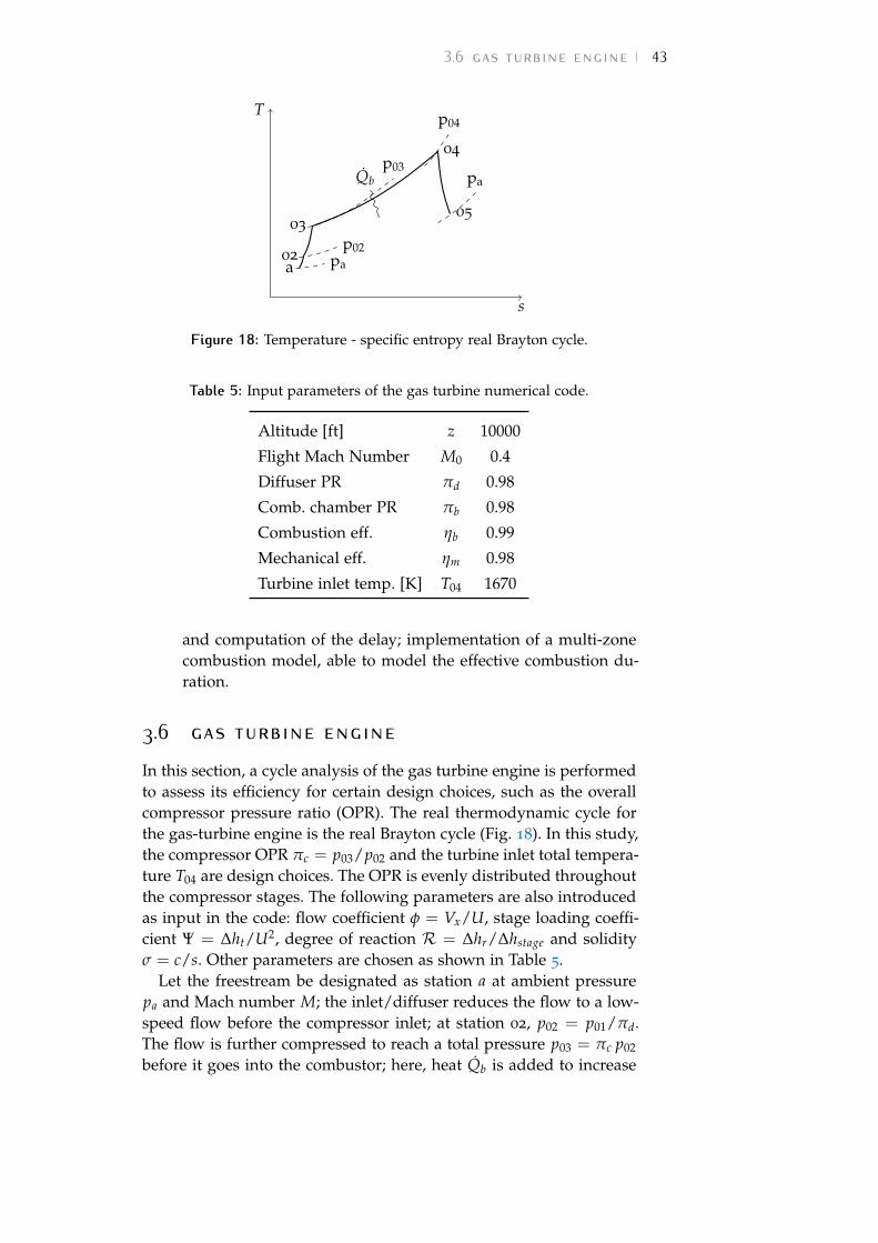
3.6 gas turbine engine 43T
s
a02
03
04
05
Qb
pa
p02
p03
p04
pa
Figure 18: Temperature - specific entropy real Brayton cycle.
Table 5: Input parameters of the gas turbine numerical code.
Altitude [ft] z 10000
Flight Mach Number M0 0.4
Diffuser PR πd 0.98
Comb. chamber PR πb 0.98
Combustion eff. ηb 0.99
Mechanical eff. ηm 0.98
Turbine inlet temp. [K] T04 1670
and computation of the delay; implementation of a multi-zonecombustion model, able to model the effective combustion du-ration.
3.6 gas turbine engineIn this section, a cycle analysis of the gas turbine engine is performedto assess its efficiency for certain design choices, such as the overallcompressor pressure ratio (OPR). The real thermodynamic cycle forthe gas-turbine engine is the real Brayton cycle (Fig. 18). In this study,the compressor OPR πc = p03/p02 and the turbine inlet total tempera-ture T04 are design choices. The OPR is evenly distributed throughoutthe compressor stages. The following parameters are also introducedas input in the code: flow coefficient φ = Vx/U, stage loading coeffi-cient Ψ = ∆ht/U2, degree of reaction R = ∆hr/∆hstage and solidityσ = c/s. Other parameters are chosen as shown in Table 5.
Let the freestream be designated as station a at ambient pressurepa and Mach number M; the inlet/diffuser reduces the flow to a low-speed flow before the compressor inlet; at station 02, p02 = p01/πd.The flow is further compressed to reach a total pressure p03 = πc p02
before it goes into the combustor; here, heat Qb is added to increase
44 thermodynamic cycle analysisthe flow temperature up to T04. A small loss in total pressure alongcombustion is accounted, as p04 = πb p03. The high temperature andpressure gas finally expands through the turbine to ambient pressurep05 = pa.
The value of OPR is of extreme importance, since it influencesthe thermal efficiency of the cycle. Apart from Rolls Royce, most ofthe aerospace companies are able to produce only two-spool engines,with OPR upper limited to 40, as the new CFM International LEAP(Leading Edge Aviation Propulsion) [7]. For this reason πc = 40 istaken as a reference value for current technology and this value isused throughout the results. As a comparison, the results obtainedby using πc = 60 will be also plotted for showing the consequencesof investing into this technology. At the present date, the only enginecapable of such performance is the new General Electric GE9X. Thefollowing assumptions have been made:
1. no air bleeding from the compressor;
2. complete expansion (p5 = pa);
3. calorically perfect gas;
4. part of the turbine power is used to drive the compressor, partto drive the propeller.
Typically a compressor and turbine have many stages with approx-imately equal pressure ratios for each stage. However, a work byA. M. Frisch [8] showed that as the size of the compressor is reduced,the compression efficiency through each stage decreases due to in-creased losses. There are four major loss mechanisms for compressors:blade surface boundary layer dissipation, wake mixing dissipation,endwall boundary layer dissipation, and tip clearance flow dissipa-tion. The efficiency loss related to these mechanisms is described in[9],[10],[11],[12]. As the size of a compressor decreases, the boundarylayer and mixing losses increase due to decreased Reynolds number.The relative tip clearance increases significantly as the compressorblade is shortened, because the absolute tip gap cannot decrease pro-portionally due to manufacturing limitations, leading to substantiallyincreased tip clearance loss. These losses strongly penalize the use ofgas-turbine engines at very low power levels.
Accounting for all these forms of losses, it is possible to computethe adiabatic efficiency for the compressor. The adiabatic efficiencyfor the compressor and turbine are defined as:
ηc =π( γ−1
γ )c − 1τc − 1
(92)
ηt =τt − 1
π( γ−1
γ )
t − 1(93)
3.6 gas turbine engine 45where τc = T03/T02, τt = T04/T05, and πt = p04/p05. The followingsteps are used in the cycle calculations.
1 . inlet and diffuser section : a-02
T02 = Ta
(1 +
γ− 12
M2)
(94)
p02 = πd pa
[1 + ηd
(T02
Ta− 1)] γ
γ−1
(95)
where γ is the air specific heat ratio, M is the flight Mach num-ber, and ηd is the adiabatic efficiency of the inlet and diffuser.
2 . compressor : 02-03 The stagnation temperature ratio can thenbe calculated starting from the OPR πc = p03/p02:
τc =T03
T02= 1 +
1ηc
(π( γ−1
γ )ecc − 1
)(96)
where ηc is the adiabatic efficiency of the compressor. The powerneeded to drive the compressor is then
Pc = ηcmacpT02(τc − 1) (97)
where ηc is the compressor isentropic efficiency, and ma is theair inlet mass flow rate.
3 . main burner : 03-04 The air-to-fuel ratio α =ma
m fcan be calcu-
lated by an energy balance at the combustor:
ηbQbm f Tm + macpT03 = (ma + m f )cpT04 (98)
α =ηbQbTm − cpT04
cp(T04 − T03)(99)
where Qb is the fuel low heating value, ηb is the combustionefficiency, and Tm is the average temperature between T03 andT04. p04 can be determined as p04 = πb p03.
4 . total turbine power : 04-a Finally, the hot gases are expandedthrough the turbine to produce enough power to drive the com-pressor and other utilities.
Pt = ηt(ma + m f )cpT04
[1−
(pa
p04
) γ−1γ]
(100)
where ηt is the turbine isentropic efficiency. The net shaft poweroutput of the turbine is Ps = Pt − Pc. The overall thermal effi-
ciency of the engine is then ηth =Ps
m f Qb.
46 thermodynamic cycle analysisPrevious works by the same authors of this work showed the benefitsof burning extra fuel in the first stages of the turbine [13],[14],[15].The so-called turbine-burner technology allows significant increasesin specific thrust (ST) with only small increases in thrust specific fuelconsumption (TSFC). Future studies might consider use of the turbineburner for the production of auxiliary power.The fuel to air ratio is computed from an energy balance at the com-bustor; inlet air lass flow air is fixed once flight Mach number andexternal conditions are known.
references[1] J. B. Heywood. Internal Combustion Engine Fundamentals. 1st ed.
II. McGraw-Hill Science/Engineering/Math, 1988. Chap. 5.
[2] T. Bose. Airbreathing Propulsion: An Introduction. Ed. by Springer-Verlag. 1st ed. Springer Aerospace Technology. New York, 2012.
[3] K. M. Chun and J. B. Heywood. “Estimating Heat-Release andMass-of-Mixture Burned from Spark-Ignition Engine PressureData.” In: Combustion Science and Technology 54 (1987), pp. 133–143.
[4] W. J. D. Annand. “Heat Transfer in the Cylinders of Reciprocat-ing Internal Combustion Engines.” In: Proceedings of the Institu-tion of Mechanical Engineers 177.36 (1963), pp. 973–996.
[5] T. Sookdeo. “Performance Measurement, Simulation, and Anal-ysis of the Cox Tee Dee 0.010, the World’s Smallest ProductionIC Engine.” Master of Science Thesis. University of Maryland,College Park, 2006.
[6] J. R. Dormand and P. J. Prince. “A Family of Embedded Runge-Kutta Formulae.” In: Journal of Computational and Applied Mathe-matics 6 (1980), pp. 19–26.
[7] CFM International. The Leap Engine. Performance. Execution. Tech-nology. Retrieved October 12, 2016. 2016. url: https://www.cfmaeroengines.com/engines/leap/.
[8] A. M. Frisch. “Scaling Effects on the Performance and Efficiencyof Gas Turbine Engines.” Master of Science Project. Universityof California, Irvine, 2014.
[9] F. M. White. Viscous Fluid Flow. New York: The McGraw-HillCompanies, Inc., 2006.
[10] D. K Hall. Performance Limits of Axial Turbomachine Stages. Tech-nical Manual. Department of Aeronautics and Astronautics, MIT.Boston, 2011.
[11] O. Sharma and T. Butler. “Predictions of Endwall Losses andSecondary Flows in Axial Flow Turbine Cascades.” In: Journalof Turbomachinery 109.2 (1987), pp. 229–236.

References 47[12] J. Denton. “The 1993 IGTI Scholar Lecture: Loss Mechanisms
in Turbomachines.” In: Journal of Turbomachinery 115.4 (1993),pp. 621–656.
[13] W. A. Sirignano and F. Liu. “Performance Increases for Gas-Turbine Engines Through Combustion Inside the Turbine.” In:Journal of Propulsion and Power 15.1 (1999), pp. 111–118.
[14] F. Liu and W. A. Sirignano. “Turbojet and Turbofan EnginePerformance Increases Through Turbine Burners.” In: Journalof Propulsion and Power 17.3 (2001), pp. 695–705.
[15] W. A. Sirignano, D. Dunn-Rankin, F. Liu, B. Colcord, and S. Pu-ranam. “Turbine Burners: Performance Improvement and Chal-lenge of Flameholding.” In: AIAA Journal 50.8 (2012), pp. 1645–1669.


Part II
R E S U LT S

4 E N G I N E S C O M PA R I S O NThe following sections will show several aircraft configurations, withengines and propellers arranged in different ways. The basic hypoth-esis behind this discussion is that the propeller efficiency is unitary.In other words, it is assumed that the propeller acts as a screw in theair without slipping, i.e. by transforming the whole input power intouseful thrust.
4.1 application of the modelsT he five numerical codes are used to compute several properties
of the engines, including thermal efficiency. As explained in theintroduction chapter 1, the power range around 100 kW is the one af-fected by low turbine efficiency. This is the result that must be reachedby each numerical model. More precisely, it was decided to investi-gate the following scenarios:
• Power equal to 75, 100, 125 and 150 kW;
• Altitude equal to 10 000, 15 000 and 20 000 feet.
By considering every combination of the five engines selected withthe parameters above, 60 simulations have been performed in total(Fig. 20-22). In order to obtain an engine with the desired power, min-imum weight and maximum efficiency, an optimization process isneeded. This process is explained here.
4.1.1 Optimization ProcessThe whole engine design allows the following parameters to be mod-ified in the numerical code:
• equivalence ratio;
• engine rpm;
• engine size (bore, stroke and n° of cylinders).
all the other variables being constant. A restriction to the efficiency-maximization process is that the equivalence ratio and the enginerpm must remain within reasonable limits for these applications, i.e.
51
52 engines comparisonΦ = 0.8− 1.5 and rpm = 1200− 5000. The optimization scheme isreported in Fig. 19.Here is an example of the optimization process. Let us consider the4-stroke spark ignition engine; assume a flight altitude (z=10 000).Cruise flight Mach is 0.4. For the IC engines in Fig. 20 and 21, thecylinder geometry (bore=8 cm, stroke=9 cm) is kept constant with al-titude and power. For a certain rpm and equivalence ratio, a power isobtained from the code: this is the power obtained from one cylinder.This power must be multiplied for an hypothetical number of cylin-ders, in order to obtain the target power of the whole engine, say 125kW. Actually, few attempts are needed to obtain exactly 125 kW. Somefiner adjustments of rpm and equivalence ratio can be done here, aswell as changing the number of cylinders. The number of cylindersincreases from 4 to 6 for powers higher than 100 kW to obtain betterefficiencies.
Once the power target is matched (within fractions of kW), thethermal efficiency of the engine can be computed by
ηth =P
m f LHV(101)
where P is the total power delivered from the engine (125 kW) andm f is the sum of the fuel consumption of every cylinder. The weightof this configuration is evaluated by means of the correlation in Sec.2, optimized with the coefficients of Table 2.1.
At this point, bore, stroke, and flight altitude are maintained con-stant, while rpm and equivalence ratio are modified. With these vari-ations, a (slightly) different efficiency is obtained, although the poweris still matching the target. The turbocharging option for altitude com-pensation allows to limit the efficiency depletion.
4.1.2 Numerical Simulations ResultsFig. 20-22 show the result of this optimization process, presenting theengines with the highest efficiency only. The results show that Dieselengines are more efficient than their gasoline counterpart, and the 4-stroke technology is more efficient than the 2-stroke; the gas turbineis the direct competitor of the 4-stroke Diesel engine from thermalefficiency viewpoint (Fig. 20).
For this reason the further discussion will be based on these two optionsonly, the others being discarded (Fig. 21-22).
Two important questions are aimed to be answered in this study.
1. Which one between Diesel engine and gas turbine is the bestchoice to accomplish a long mission?
2. Which engine-propeller layout (number, connections, size) givesthe best performance?
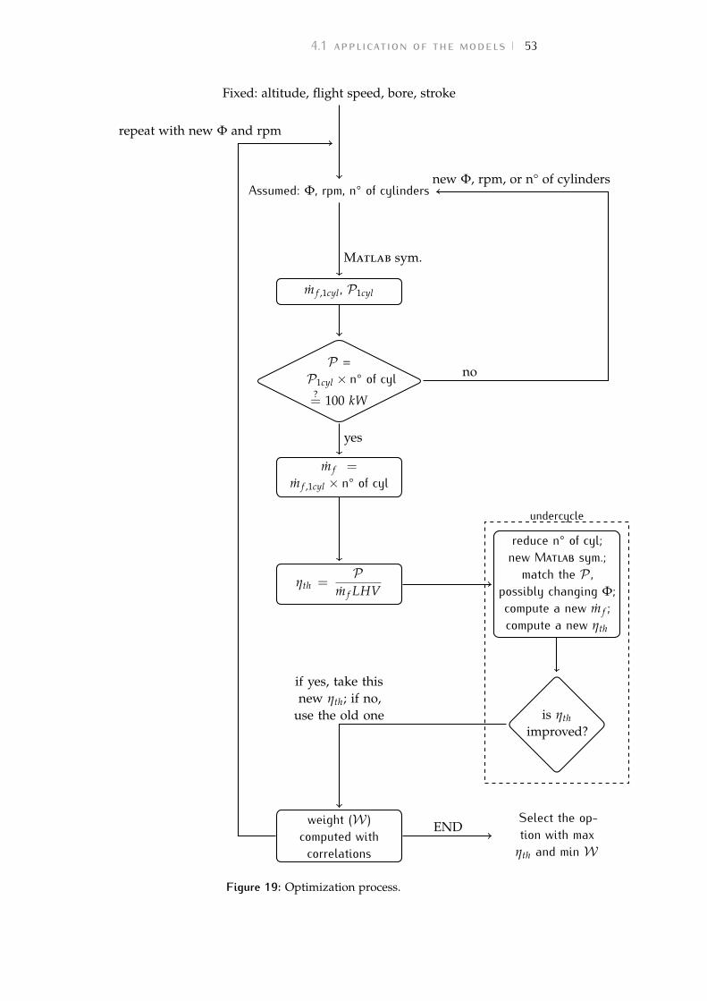
4.1 application of the models 53Fixed: altitude, flight speed, bore, stroke
Assumed: Φ, rpm, n° of cylinders
m f ,1cyl , P1cyl
P =P1cyl × n° of cyl
?= 100 kW
m f =
m f ,1cyl × n° of cyl
ηth =P
m f LHV
reduce n° of cyl;new Matlab sym.;match the P ,possibly changing Φ;compute a new m f ;compute a new ηth
if yes, take thisnew ηth; if no,
use the old one is ηthimproved?
weight (W )computed withcorrelationsSelect the op-tion with max
ηth and min W
Matlab sym.
yes
no
new Φ, rpm, or n° of cylinders
undercycle
END
repeat with new Φ and rpm
Figure 19: Optimization process.
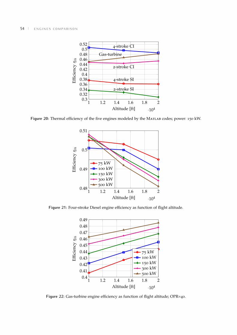
54 engines comparison
1 1.2 1.4 1.6 1.8 2
·104
0.30.320.340.360.380.4
0.420.440.460.480.5
0.52
4-stroke SI
4-stroke CI
2-stroke SI
2-stroke CI
Gas-turbine
Altitude [ft]
Effic
ienc
yη
th
Figure 20: Thermal efficiency of the five engines modeled by the Matlab codes; power: 150 kW.
1 1.2 1.4 1.6 1.8 2
·104
0.48
0.49
0.5
0.51
Altitude [ft]
Effic
ienc
yη
th
75 kW100 kW150 kW300 kW500 kW
Figure 21: Four-stroke Diesel engine efficiency as function of flight altitude.
1 1.2 1.4 1.6 1.8 2
·104
0.40.410.420.430.440.450.460.470.480.49
Altitude [ft]
Effic
ienc
yη
th
75 kW100 kW150 kW300 kW500 kW
Figure 22: Gas-turbine engine efficiency as function of flight altitude; OPR=40.
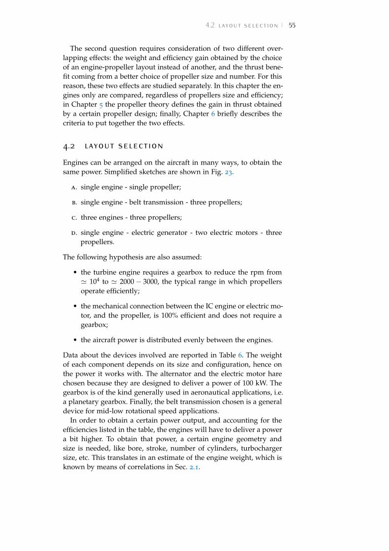
4.2 layout selection 55The second question requires consideration of two different over-
lapping effects: the weight and efficiency gain obtained by the choiceof an engine-propeller layout instead of another, and the thrust bene-fit coming from a better choice of propeller size and number. For thisreason, these two effects are studied separately. In this chapter the en-gines only are compared, regardless of propellers size and efficiency;in Chapter 5 the propeller theory defines the gain in thrust obtainedby a certain propeller design; finally, Chapter 6 briefly describes thecriteria to put together the two effects.
4.2 layout selectionEngines can be arranged on the aircraft in many ways, to obtain thesame power. Simplified sketches are shown in Fig. 23.
a. single engine - single propeller;
b. single engine - belt transmission - three propellers;
c. three engines - three propellers;
d. single engine - electric generator - two electric motors - threepropellers.
The following hypothesis are also assumed:
• the turbine engine requires a gearbox to reduce the rpm from' 104 to ' 2000− 3000, the typical range in which propellersoperate efficiently;
• the mechanical connection between the IC engine or electric mo-tor, and the propeller, is 100% efficient and does not require agearbox;
• the aircraft power is distributed evenly between the engines.
Data about the devices involved are reported in Table 6. The weightof each component depends on its size and configuration, hence onthe power it works with. The alternator and the electric motor harechosen because they are designed to deliver a power of 100 kW. Thegearbox is of the kind generally used in aeronautical applications, i.e.a planetary gearbox. Finally, the belt transmission chosen is a generaldevice for mid-low rotational speed applications.
In order to obtain a certain power output, and accounting for theefficiencies listed in the table, the engines will have to deliver a powera bit higher. To obtain that power, a certain engine geometry andsize is needed, like bore, stroke, number of cylinders, turbochargersize, etc. This translates in an estimate of the engine weight, which isknown by means of correlations in Sec. 2.1.
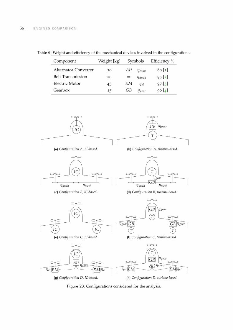
56 engines comparison
Table 6: Weight and efficiency of the mechanical devices involved in the configurations.
Component Weight [kg] Symbols Efficiency %
Alternator Converter 10 Alt ηconv 80 [1]
Belt Transmission 20 = ηmech 95 [2]
Electric Motor 45 EM ηel 97 [3]
Gearbox 15 GB ηgear 90 [4]
IC
(a) Configuration A, IC-based.
T
GB ηgear
(b) Configuration A, turbine-based.
IC
ηmech ηmech
(c) Configuration B, IC-based.
T
GBηgear
ηmech ηmech
(d) Configuration B, turbine-based.
IC
IC
IC
(e) Configuration C, IC-based.
GBηgear
T
T
GB ηgear
GB ηgear
T(f ) Configuration C, turbine-based.
EMηel
IC
Alt ηconvEM ηel
(g) Configuration D, IC-based.
EMηel
T
GB ηgear
Alt ηconvEM ηel
(h) Configuration D, turbine-based.
Figure 23: Configurations considered for the analysis.
4.2 layout selection 57Concerning the Diesel-based configurations, the lightest is always
the one with one single large engine driving its own propeller (con-figuration A). This arrangement is the lightest because it does notrequire any additional weight from belt transmissions or alternators,as in the other configurations. Moreover, the number of componentsconstituting the working chain is minimum, so the product of ineffi-ciencies is not deteriorated as it would be with a large number ofelements.1 On so doing, the engine must deliver less power to obtainthe desired power output, implying less fuel consumption.
Compared to A:
• configuration B requires the use of the transmission, which addsweight and inefficiency to the whole system. Hence, there is theneed of a slightly more powerful engine and additional weight;
• since the weight of an IC engine do not scale linearly withpower, the use of 3 smaller engines in configurations C resultsheavier and less efficient;
• the transformation from mechanical energy to electrical energyis the main source of inefficiency, which translates in a largerengine needed to provide the same output power. Hybrid con-figuration D is the heaviest among the four, mainly because ofthe higher fuel consumption and also, of lesser importance, be-cause of the higher weight of the components.
The same considerations apply for the turbine-based configurations.In other words, the lightest configuration is still the one with one sin-gle large turbine driving a propeller; however, the large difference inthe rotational speed of the two shafts requires the use of a gearedconnection between the two parts. The lightness of the turbine is thencompensated by the additional weight of the gearbox. The fuel con-sumption of the three-turbines, three-propellers configuration C ishigher than the one with one engine only, due to the scale effects.The smaller is the turbine, the less efficient it is. Moreover, the sum ofthree small turbines exceeds the weight of a single bigger turbine, fortwo reasons: the presence of three gearboxes instead of one, and thenon-linear relation between power and weight.
4.2.1 Altitude Compensation and Flammability LimitsIf the flight altitude changes, the environmental conditions change aswell. The main consequence on the engine is the so called density effect:as the altitude increases, the air density decreases, and the intake
1 In a mechanical system, the efficiency of the whole system depends on the efficiencyof the single element constituting the chain and on the way they are assembled. Ifthe elements are arranged in series, the overall efficiency of the system is given bythe product of each single element efficiency: η = η1 · η2 · · · ηn.
58 engines comparisonmanifold, for a fixed cross section area and airspeed velocity, ingestsless air. As a result, the machine operates with lower working charge,either it is a internal combustion engine or a turbine engine. On theother hand, the combustion process requires the equivalence ratioΦ to be within the flammability limits, in order to obtain a propercombustion. Hence, for a fixed Φ the fuel amount that is possible toinject is lower than it would be at lower altitude. Since P ∝ m f W,lower power is obtained.
The ignition range of a mixture depends on pressure, chamber ar-chitecture and the couple oxidizer-fuel adopted. As a general trend,by decreasing the pressure, the range becomes narrower and the mix-ing requirement more stringent. Spark-ignition (SI) engines usuallyoperate stoichiometric or slightly rich, while compression-ignition(CI) engines operate slightly or very lean. In SI engines the freshcharge is composed by a premixed mixture of air and fuel. The sparkignites the charge when proper conditions of pressure, temperature,mixing and Φ are present in the combustion chamber. The upper limitfor the pressure is the one dictated by the engine knocking. Knock oc-curs when combustion of the air/fuel mixture in the cylinder doesnot start off correctly in response to ignition by the spark plug, butone or more pockets of air/fuel mixture explode outside the enve-lope of the normal combustion front. CI engines, instead, are not tiedto knocking, since the charge is composed by air only and can notignite unless fuel in injected. Moreover, every hydrocarbon fuel hasits own Carbon and Hydrogen content, which corresponds to a dif-ferent amount of Oxygen required for burning. If an amount of air isstoichiometric for a certain fuel, it may be lean or rich for a differentfuel. Finally, the value of Φ with which the engine operates is alsodictated by environmental regulations in order to control the exhaustpollutants.
Since Φ is bounded by the reasons mentioned above, often theturbocharging option is adopted. By the introduction of an higheramount of air with respect to the one naturally aspirated by the engine,it is possible to inject more fuel still maintaining the correct equiva-lence ratio. By acting on the turbocharger’s rpm, it is then possible totune the engine power to the desired value.
This is the reason why the engines’ size and geometry2 are keptconstant with altitude, and so are their powers, by means of actingon the turbocharger and the engine rpm. As a drawback, the engine’sfuel consumption and thermal efficiency change with altitude. Thesevalues as a function of flight altitude are shown in Table 7.
2 Hence, the weight.
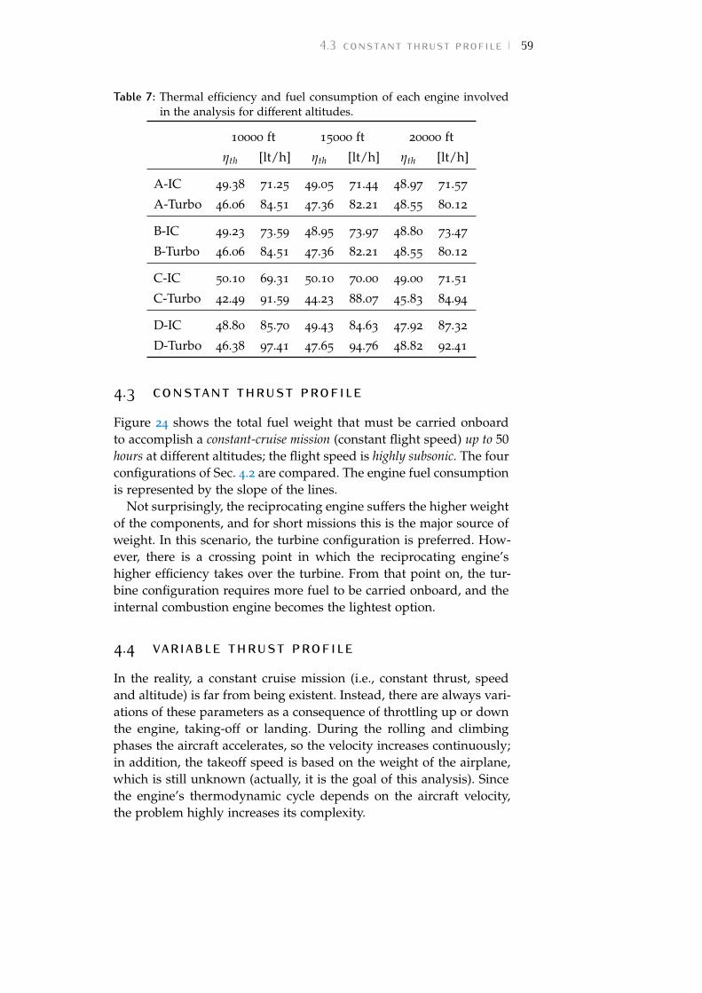
4.3 constant thrust profile 59Table 7: Thermal efficiency and fuel consumption of each engine involved
in the analysis for different altitudes.
10000 ft 15000 ft 20000 ft
ηth [lt/h] ηth [lt/h] ηth [lt/h]
A-IC 49.38 71.25 49.05 71.44 48.97 71.57
A-Turbo 46.06 84.51 47.36 82.21 48.55 80.12
B-IC 49.23 73.59 48.95 73.97 48.80 73.47
B-Turbo 46.06 84.51 47.36 82.21 48.55 80.12
C-IC 50.10 69.31 50.10 70.00 49.00 71.51
C-Turbo 42.49 91.59 44.23 88.07 45.83 84.94
D-IC 48.80 85.70 49.43 84.63 47.92 87.32
D-Turbo 46.38 97.41 47.65 94.76 48.82 92.41
4.3 constant thrust profileFigure 24 shows the total fuel weight that must be carried onboardto accomplish a constant-cruise mission (constant flight speed) up to 50hours at different altitudes; the flight speed is highly subsonic. The fourconfigurations of Sec. 4.2 are compared. The engine fuel consumptionis represented by the slope of the lines.
Not surprisingly, the reciprocating engine suffers the higher weightof the components, and for short missions this is the major source ofweight. In this scenario, the turbine configuration is preferred. How-ever, there is a crossing point in which the reciprocating engine’shigher efficiency takes over the turbine. From that point on, the tur-bine configuration requires more fuel to be carried onboard, and theinternal combustion engine becomes the lightest option.
4.4 variable thrust profileIn the reality, a constant cruise mission (i.e., constant thrust, speedand altitude) is far from being existent. Instead, there are always vari-ations of these parameters as a consequence of throttling up or downthe engine, taking-off or landing. During the rolling and climbingphases the aircraft accelerates, so the velocity increases continuously;in addition, the takeoff speed is based on the weight of the airplane,which is still unknown (actually, it is the goal of this analysis). Sincethe engine’s thermodynamic cycle depends on the aircraft velocity,the problem highly increases its complexity.
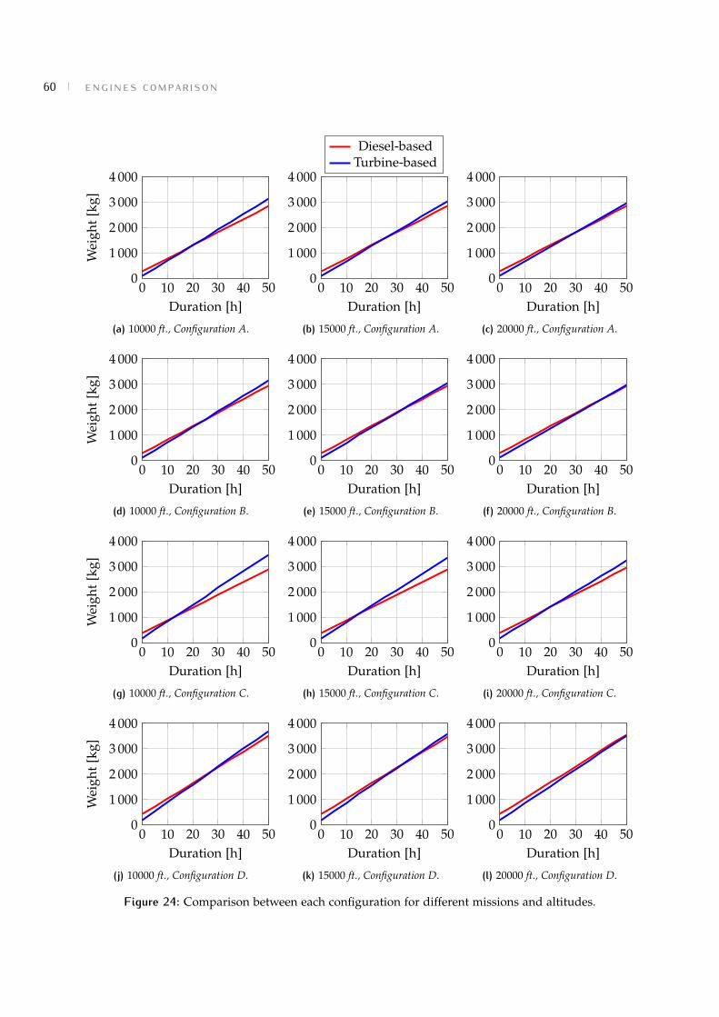
60 engines comparison
0 10 20 30 40 500
1 000
2 000
3 000
4 000
Duration [h]
Wei
ght
[kg]
(a) 10000 ft., Configuration A.
0 10 20 30 40 500
1 000
2 000
3 000
4 000
Duration [h]
Diesel-basedTurbine-based
(b) 15000 ft., Configuration A.
0 10 20 30 40 500
1 000
2 000
3 000
4 000
Duration [h]
(c) 20000 ft., Configuration A.
0 10 20 30 40 500
1 000
2 000
3 000
4 000
Duration [h]
Wei
ght
[kg]
(d) 10000 ft., Configuration B.
0 10 20 30 40 500
1 000
2 000
3 000
4 000
Duration [h]
(e) 15000 ft., Configuration B.
0 10 20 30 40 500
1 000
2 000
3 000
4 000
Duration [h]
(f ) 20000 ft., Configuration B.
0 10 20 30 40 500
1 000
2 000
3 000
4 000
Duration [h]
Wei
ght
[kg]
(g) 10000 ft., Configuration C.
0 10 20 30 40 500
1 000
2 000
3 000
4 000
Duration [h]
(h) 15000 ft., Configuration C.
0 10 20 30 40 500
1 000
2 000
3 000
4 000
Duration [h]
(i) 20000 ft., Configuration C.
0 10 20 30 40 500
1 000
2 000
3 000
4 000
Duration [h]
Wei
ght
[kg]
(j) 10000 ft., Configuration D.
0 10 20 30 40 500
1 000
2 000
3 000
4 000
Duration [h]
(k) 15000 ft., Configuration D.
0 10 20 30 40 500
1 000
2 000
3 000
4 000
Duration [h]
(l) 20000 ft., Configuration D.
Figure 24: Comparison between each configuration for different missions and altitudes.
4.4 variable thrust profile 61Changes in aircraft velocity and/or thrust can be assessed together
by looking at the engine’s power. If variations of power are intro-duced in the mission, for whichever reason, two levels of simplifica-tion are possible:
1. the more rigorous way to proceed would be to iterate on thefuel weight, assuming a guess value m0 (for instance the weightgiven by a chosen constant-thrust mission from Section 4.3).Along the mission, the weight reduces continuously by the burn-ing of the fuel: the weight at a generic moment t is:
m(t) = m0 −∫ t
0m f (t)dt (102)
where m f (t) is the instantaneous fuel consumption, unknown.3
Moreover, during the climbing phase the altitude changes con-tinuously, hence the engine keeps working with changing inletconditions. Hence it is
m f = m f (z, m(t),P) (103)
which makes the problem strongly coupled. Eq. 102 and 103,together with models for the aircraft trajectory, definitions ofthrust, drag and lift, plus appropriate boundary conditions, con-stitute a differential problem that can be solved by means ofnumerical methods, such as finite differences.
The iteration takes place if the mass of the fuel reaches zero be-fore the end of the mission, whose length has been fixed whenm0 was chosen; in this case, a different value of m0 is needed torestart the computations.
2. a much simpler approach is to neglect the dependence of thefuel consumption by the altitude and the instantaneous weightof the aircraft, i.e.
m f = m f (P). (104)
Although very strong, this hypothesis suggests that the fuel con-sumption depends on the engine throttling only. In other words,this simplification consists in the study of a flying aircraft whoseengine keeps working on the ground, with constant inlet condi-tions. This approach clearly overestimates the fuel consumption:in fact, the thermodynamic cycle becomes more efficient as theexternal temperature decreases, hence when flying at higher al-titudes. The results of this analysis are influenced by this hy-pothesis, but, although overestimated, they still provide a suffi-cient accuracy.
The value m f can be obtained by the Matlab numerical codedeveloped for this study and described in Chap. 3, once the
3 Note that m0 = mstruct + mpayload + mengine + m f uel .
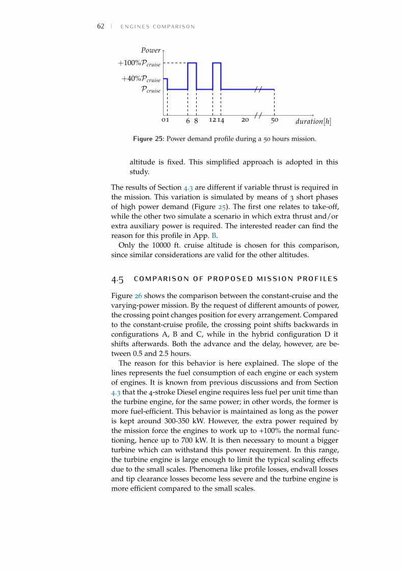
62 engines comparisonPower
0 duration[h]
+100%Pcruise
+40%Pcruise
Pcruise
1 6 8 1214 20 50//
//
Figure 25: Power demand profile during a 50 hours mission.
altitude is fixed. This simplified approach is adopted in thisstudy.
The results of Section 4.3 are different if variable thrust is required inthe mission. This variation is simulated by means of 3 short phasesof high power demand (Figure 25). The first one relates to take-off,while the other two simulate a scenario in which extra thrust and/orextra auxiliary power is required. The interested reader can find thereason for this profile in App. B.
Only the 10000 ft. cruise altitude is chosen for this comparison,since similar considerations are valid for the other altitudes.
4.5 comparison of proposed mission profilesFigure 26 shows the comparison between the constant-cruise and thevarying-power mission. By the request of different amounts of power,the crossing point changes position for every arrangement. Comparedto the constant-cruise profile, the crossing point shifts backwards inconfigurations A, B and C, while in the hybrid configuration D itshifts afterwards. Both the advance and the delay, however, are be-tween 0.5 and 2.5 hours.
The reason for this behavior is here explained. The slope of thelines represents the fuel consumption of each engine or each systemof engines. It is known from previous discussions and from Section4.3 that the 4-stroke Diesel engine requires less fuel per unit time thanthe turbine engine, for the same power; in other words, the former ismore fuel-efficient. This behavior is maintained as long as the poweris kept around 300-350 kW. However, the extra power required bythe mission force the engines to work up to +100% the normal func-tioning, hence up to 700 kW. It is then necessary to mount a biggerturbine which can withstand this power requirement. In this range,the turbine engine is large enough to limit the typical scaling effectsdue to the small scales. Phenomena like profile losses, endwall lossesand tip clearance losses become less severe and the turbine engine ismore efficient compared to the small scales.
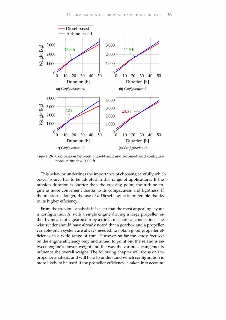
4.5 comparison of proposed mission profiles 63
0 10 20 30 40 500
1 000
2 000
3 00017.5 h
Duration [h]
Wei
ght
[kg]
Diesel-basedTurbine-based
(a) Configuration A.
0 10 20 30 40 500
1 000
2 000
3 00022.5 h
Duration [h]
(b) Configuration B.
0 10 20 30 40 500
1 000
2 000
3 000
4 000
12 h
Duration [h]
Wei
ght
[kg]
(c) Configuration C.
0 10 20 30 40 500
1 000
2 000
3 000
4 000
28.5 h
Duration [h]
(d) Configuration D.
Figure 26: Comparison between Diesel-based and turbine-based configura-tions. Altitude=10000 ft.
This behavior underlines the importance of choosing carefully whichpower source has to be adopted in this range of applications. If themission duration is shorter than the crossing point, the turbine en-gine is more convenient thanks to its compactness and lightness. Ifthe mission is longer, the use of a Diesel engine is preferable thanksto its higher efficiency.
From the previous analysis it is clear that the most appealing layoutis configuration A, with a single engine driving a large propeller, ei-ther by means of a gearbox or by a direct mechanical connection. Thewise reader should have already noted that a gearbox and a propellervariable-pitch system are always needed, to obtain good propeller ef-ficiency in a wide range of rpm. However, so far the study focusedon the engine efficiency only and aimed to point out the relations be-tween engine’s power, weight and the way the various arrangementsinfluence the overall weight. The following chapter will focus on thepropeller analysis, and will help to understand which configuration ismore likely to be used if the propeller efficiency is taken into account.
64 engines comparisonreferences[1] R. Bosch GmbH. Automotive Handbook. 8th ed. pag. 993. printed
in Germany: Horst Bauer, 2011.
[2] Inc. Carlisle Power Transmission Products. Energy Loss and Effi-ciency of Power Transmission Belts. Ed. by Belt Technical Center.Springfield, Missouri, 2009.
[3] EVDrive motors. High Performance EVD Motor/Controller IP67Drive Sub-Systems. Ed. by EVDrive Research. Portland, Oregon,2016.
[4] B. R. Höhn, K. Stahl, and P. Gwinner. “Light-Weight Design forPlanetary Gear Transmissions.” In: Geartechnology (2013). Ed. byRandall Publications LLC.
5 P R O P E L L E R A N A LY S I S5.1 momentum theoryT he efficiency of a piston engine-propeller combination depends
on a proper match of the propeller to the engine as well as amatch of the two to the airframe; aerodynamically, one strives to se-lect a propeller that provides a high efficiency for cruise and a highstatic thrust for take-off. These two requirements are easier to satisfywith a variable pitch propeller. A fixed pitch propeller is usually acompromise between these two operating regimes. The terms con-stant pitch, fixed pitch and variable pitch are somewhat confusing. Aconstant pitch propeller is one whose pitch does not vary with radius."Fixed" or "variable" pitch refers to whether or not the whole bladecan rotate about an axis along the blade in order to vary the pitchangles of the blade sections all along the blade (this is called feath-ering). Some propellers are equipped with governors to maintain aconstant rpm as the engine throttle is varied. This is done by increas-ing the blade pitch angles as the propeller rpm tends to increase dueto increased power or, vice versa, by decreasing the pitch for reducedpower. Such propeller is called a "constant speed" propeller [1].
According to the early literature a propeller can be seen as an"airscrew" which screws itself through the surrounding air. By apply-ing the classical momentum theory to a control volume including theactuating disc and its surroundings, an important result is obtained:
P = T (V + w) (105)
where T is the thrust, P is the power, V is the true airspeed and wis the induced velocity. This important result states that the powerrequired by the propeller equals the product of its thrust and thevelocity through the propeller. This can be divided into two parts. Thefirst part is defined as the useful power:
Pu = T V . (106)
The second part is known as the induced power:
Pi = T w. (107)
65
66 propeller analysisThe induced velocity is given by the relation ([1], chap. 6):
w =12
[− V +
√V2 +
(2TρA
) ](108)
where ρ is the air density at the local altitude and A is the disc area.In forward flight, an ideal efficiency can be defined as the ratio of theuseful power to the total power:
ηid =T V
T (V + w)=
11 + (w/V) . (109)
It is interesting to note that, as V increases, the ideal efficiency is seento approach unity. By applying typical numbers to Eq. 109 it is easy toobtain efficiencies around 95%. However, ηid given by the momentumtheory is optimistic and represents an upper limit that is really notattainable: with the same numbers, the actual propeller efficiency iscloser to 85%.
At low speeds (e.g., during the take-off roll), the efficiency is diffi-cult to estimate. At zero forward speed, the efficiency of a propelleris zero by definition, even though its thrust is not zero. In fact, for thesame shaft power, a variable pitch propeller will produce the mostthrust at zero advance velocity (i.e., its static thrust is greater than thethrust produced in forward flight).
5.2 momentum - blade element approximatedtheoryMore reliable evaluations of propeller efficiency are attainable if theblade theory is considered, which is described in detail in [1] and isbriefly outlined here.
The thrust and the power of a propeller are normally expressedin coefficient form. These non-dimensional coefficients are definedin various ways, depending on what particular reference areas andvelocities are used. Test results on propellers almost always definethe thrust coefficient, CT, and power coefficient, CP, as follows:
CT =T
ρn2D4 (110a)
CP =P
ρn3D5 (110b)
where n is the rotational speed in revolutions per second and D isthe propeller diameter. All the others quantities must be expressed inconsistent units. One of the most famous coefficient used in propelleranalysis is the advance ratio J, defined by
J =V
nD. (111)
5.2 momentum - blade element approximated theory 67Thus, CT and CP are functions of J. The classical definition of pro-peller efficiency (analogous to Eq. 109)
ηprop =T VP (112)
can be also expressed in terms of CT, CP and J, becoming
ηprop =CT JCP
. (113)
Equations 110 are very convenient to have a quick description of apropeller behavior. However, they don’t take into account the realaerodynamics of the blades. The value of thrust, for example, de-pends on the distribution of the aerodynamic forces of the blade andon the blade pitch, angle of attack, rpm, geometry and length. Thrustis strictly connected to the lift formation; however, since the pressuredifference across the blades must vanish at the tips, lift vanishes atthe tips too, which generally means that the local angle of attack atthe tip must be zero. A trailing vortex system, helical in shape, isgenerated by the propeller in a manner similar to a finite wing. Con-siderations on the induced velocity and on the wake created by thefluid-structure interaction also apply. In fact, the propeller does notbehave as a perfect "airscrew", but slips partially when screwing intothe air stream; tangential components induced on the downstreamair translate in the formation of a wake. Turbulent structures and vor-ticity in the wake imply additional drag, hence more thrust is neededto compensate it.
Equations 110 can be applied to a blade element and integratedalong the radius accounting for the blade geometry and the local airstream properties. This process may require a few iterations and theaid of a numerical solver. Some useful relationships are reported hereby applying some fairly accurate approximation. CT and CP become
CT =π3σ
24CL f (λ) (114a)
CP = JCT +π4σ
8CDg(λ). (114b)
whereσ =
BcπL λ =
VωL (115)
f (λ) =(
1 + λ2) 3
2 − λ3 (116)
g(λ) =12
[(1 + λ2
)2(2 + λ2
)− λ4 log
1 +√
1 + λ2
λ
]. (117)
CL and CD indicate average values of lift and drag coefficient respec-tively, B is the number of blades, c is a reference chord length, L is
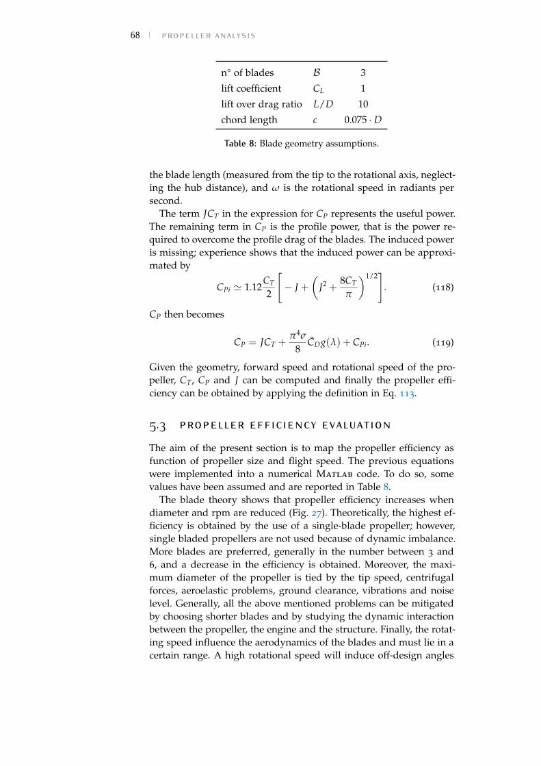
68 propeller analysisn° of blades B 3
lift coefficient CL 1
lift over drag ratio L/D 10
chord length c 0.075 · D
Table 8: Blade geometry assumptions.
the blade length (measured from the tip to the rotational axis, neglect-ing the hub distance), and ω is the rotational speed in radiants persecond.
The term JCT in the expression for CP represents the useful power.The remaining term in CP is the profile power, that is the power re-quired to overcome the profile drag of the blades. The induced poweris missing; experience shows that the induced power can be approxi-mated by
CPi ' 1.12CT
2
[− J +
(J2 +
8CT
π
)1/2]
. (118)
CP then becomes
CP = JCT +π4σ
8CDg(λ) + CPi. (119)
Given the geometry, forward speed and rotational speed of the pro-peller, CT, CP and J can be computed and finally the propeller effi-ciency can be obtained by applying the definition in Eq. 113.
5.3 propeller efficiency evaluationThe aim of the present section is to map the propeller efficiency asfunction of propeller size and flight speed. The previous equationswere implemented into a numerical Matlab code. To do so, somevalues have been assumed and are reported in Table 8.
The blade theory shows that propeller efficiency increases whendiameter and rpm are reduced (Fig. 27). Theoretically, the highest ef-ficiency is obtained by the use of a single-blade propeller; however,single bladed propellers are not used because of dynamic imbalance.More blades are preferred, generally in the number between 3 and6, and a decrease in the efficiency is obtained. Moreover, the maxi-mum diameter of the propeller is tied by the tip speed, centrifugalforces, aeroelastic problems, ground clearance, vibrations and noiselevel. Generally, all the above mentioned problems can be mitigatedby choosing shorter blades and by studying the dynamic interactionbetween the propeller, the engine and the structure. Finally, the rotat-ing speed influence the aerodynamics of the blades and must lie in acertain range. A high rotational speed will induce off-design angles
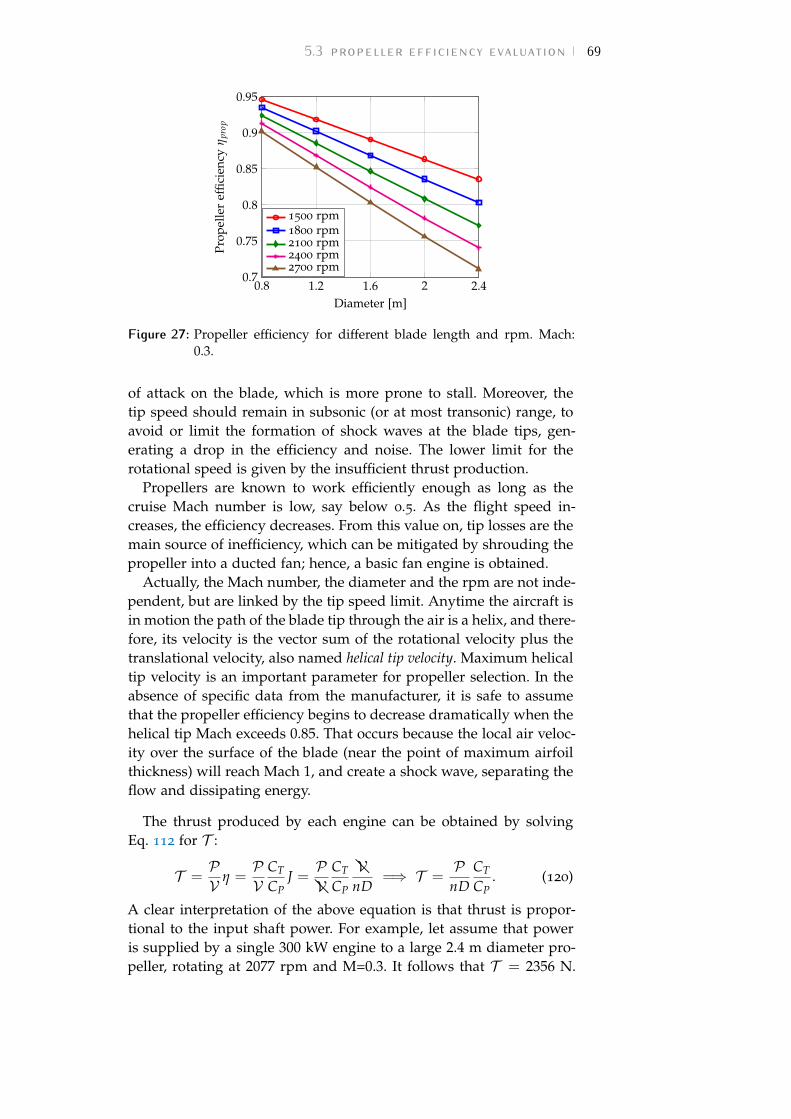
5.3 propeller efficiency evaluation 69
0.8 1.2 1.6 2 2.40.7
0.75
0.8
0.85
0.9
0.95
Diameter [m]
Prop
elle
ref
ficie
ncy
ηpr
op1500 rpm1800 rpm2100 rpm2400 rpm2700 rpm
Figure 27: Propeller efficiency for different blade length and rpm. Mach:0.3.
of attack on the blade, which is more prone to stall. Moreover, thetip speed should remain in subsonic (or at most transonic) range, toavoid or limit the formation of shock waves at the blade tips, gen-erating a drop in the efficiency and noise. The lower limit for therotational speed is given by the insufficient thrust production.
Propellers are known to work efficiently enough as long as thecruise Mach number is low, say below 0.5. As the flight speed in-creases, the efficiency decreases. From this value on, tip losses are themain source of inefficiency, which can be mitigated by shrouding thepropeller into a ducted fan; hence, a basic fan engine is obtained.
Actually, the Mach number, the diameter and the rpm are not inde-pendent, but are linked by the tip speed limit. Anytime the aircraft isin motion the path of the blade tip through the air is a helix, and there-fore, its velocity is the vector sum of the rotational velocity plus thetranslational velocity, also named helical tip velocity. Maximum helicaltip velocity is an important parameter for propeller selection. In theabsence of specific data from the manufacturer, it is safe to assumethat the propeller efficiency begins to decrease dramatically when thehelical tip Mach exceeds 0.85. That occurs because the local air veloc-ity over the surface of the blade (near the point of maximum airfoilthickness) will reach Mach 1, and create a shock wave, separating theflow and dissipating energy.
The thrust produced by each engine can be obtained by solvingEq. 112 for T :
T =PV η =
PV
CT
CPJ =P@@V
CT
CP
@@VnD
=⇒ T =P
nDCT
CP. (120)
A clear interpretation of the above equation is that thrust is propor-tional to the input shaft power. For example, let assume that poweris supplied by a single 300 kW engine to a large 2.4 m diameter pro-peller, rotating at 2077 rpm and M=0.3. It follows that T = 2356 N.
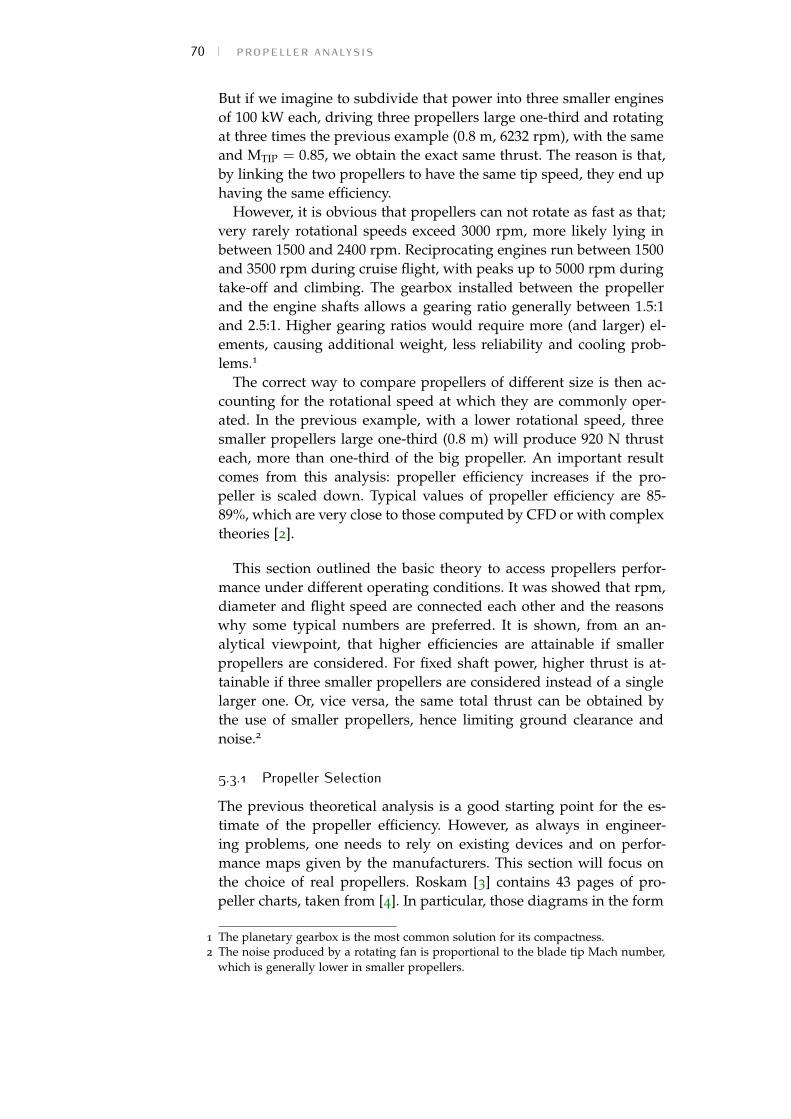
70 propeller analysisBut if we imagine to subdivide that power into three smaller enginesof 100 kW each, driving three propellers large one-third and rotatingat three times the previous example (0.8 m, 6232 rpm), with the sameand MTIP = 0.85, we obtain the exact same thrust. The reason is that,by linking the two propellers to have the same tip speed, they end uphaving the same efficiency.
However, it is obvious that propellers can not rotate as fast as that;very rarely rotational speeds exceed 3000 rpm, more likely lying inbetween 1500 and 2400 rpm. Reciprocating engines run between 1500and 3500 rpm during cruise flight, with peaks up to 5000 rpm duringtake-off and climbing. The gearbox installed between the propellerand the engine shafts allows a gearing ratio generally between 1.5:1and 2.5:1. Higher gearing ratios would require more (and larger) el-ements, causing additional weight, less reliability and cooling prob-lems.1
The correct way to compare propellers of different size is then ac-counting for the rotational speed at which they are commonly oper-ated. In the previous example, with a lower rotational speed, threesmaller propellers large one-third (0.8 m) will produce 920 N thrusteach, more than one-third of the big propeller. An important resultcomes from this analysis: propeller efficiency increases if the pro-peller is scaled down. Typical values of propeller efficiency are 85-89%, which are very close to those computed by CFD or with complextheories [2].
This section outlined the basic theory to access propellers perfor-mance under different operating conditions. It was showed that rpm,diameter and flight speed are connected each other and the reasonswhy some typical numbers are preferred. It is shown, from an an-alytical viewpoint, that higher efficiencies are attainable if smallerpropellers are considered. For fixed shaft power, higher thrust is at-tainable if three smaller propellers are considered instead of a singlelarger one. Or, vice versa, the same total thrust can be obtained bythe use of smaller propellers, hence limiting ground clearance andnoise.2
5.3.1 Propeller SelectionThe previous theoretical analysis is a good starting point for the es-timate of the propeller efficiency. However, as always in engineer-ing problems, one needs to rely on existing devices and on perfor-mance maps given by the manufacturers. This section will focus onthe choice of real propellers. Roskam [3] contains 43 pages of pro-peller charts, taken from [4]. In particular, those diagrams in the form
1 The planetary gearbox is the most common solution for its compactness.2 The noise produced by a rotating fan is proportional to the blade tip Mach number,
which is generally lower in smaller propellers.
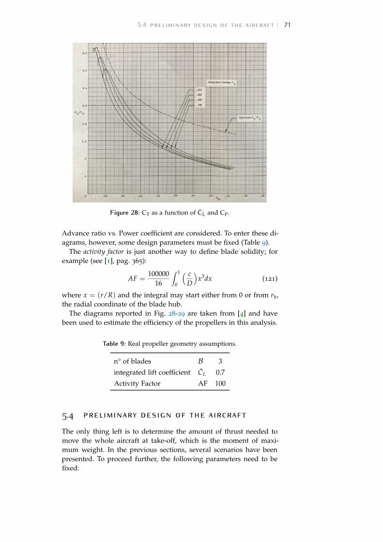
5.4 preliminary design of the aircraft 71
Figure 28: CT as a function of CL and CP.
Advance ratio vs. Power coefficient are considered. To enter these di-agrams, however, some design parameters must be fixed (Table 9).
The activity factor is just another way to define blade solidity; forexample (see [1], pag. 365):
AF =100000
16
∫ 1
0
( cD
)x3dx (121)
where x = (r/R) and the integral may start either from 0 or from rh,the radial coordinate of the blade hub.
The diagrams reported in Fig. 28-29 are taken from [4] and havebeen used to estimate the efficiency of the propellers in this analysis.
Table 9: Real propeller geometry assumptions.
n° of blades B 3
integrated lift coefficient CL 0.7
Activity Factor AF 100
5.4 preliminary design of the aircraftThe only thing left is to determine the amount of thrust needed tomove the whole aircraft at take-off, which is the moment of maxi-mum weight. In the previous sections, several scenarios have beenpresented. To proceed further, the following parameters need to befixed:
72 propeller analysis
Figure 29: Propeller efficiency as a function of J and CP.
• engine(s) power profile for the whole mission;
• mission duration;
• engine technology (Diesel or gas-turbine) and n°.
On so doing, the weight of the fuel W f uel needed to accomplish themission should be known. Moreover, the weight of the engines Wenginecan be computed by means of correlations. The overall weight of theaircraft at take-off includes also the weight of the structure and thepayload, which need to be modeled.
In his work, Raymer [5] suggests a procedure to estimate the "De-sign take-off gross weight", which is defined as the total weight of theaircraft as it begins the mission for which it was designed3. Designtake-off gross weight can be divided into crew weight, payload (orpassenger) weight, fuel weight, and empty weight. The empty weightincludes the structure, engines, landing gear, fixed equipment, avion-ics and anything else not considered a part of crew, payload or fuel.Eq. 122 summarizes the take-off weight buildup:
W0 =Wcrew +Wpayload +W f uel +We. (122)
Being a UAV the target of this analysis, no crew is involved inthe mission. The payload, not well defined yet, might be composedby electronic devices like cameras, avionics systems or weapons. De-pending on the mission, it can be considered as an external input.Hence,
W0 =Wpayload +W f uel +We (123)
3 This is not necessarily the same as the "maximum take-off weight". In fact, many mil-itary aircraft can be overloaded beyond design weight, yet suffering from a reducedmaneuverability.
5.4 preliminary design of the aircraft 73The only unknown is the empty weight, which is a function of
the total aircraft weight itself W0. To simplify calculations, the emptyweight can be expressed as a fraction of the total takeoff weight, i.e.
W0 =Wpayload +W f uel +
(We
W0
)W0. (124)
The empty-weight fraction We/W0 can be estimated statisticallyfrom historical trends; data are shown in [5] and are fitted so thatcorrelations are obtained. These fractions vary from about 0.3 and0.7, and diminish with increasing total aircraft weight. Flying boatshave the highest empty-weight fraction, long-range military aircrafthave the lowest. This dependence can be expressed by the exponentialequation (weights are expressed in pounds):
We
W0= aW b
0 (125)
where a and b are coefficients depending on aircraft mission andsize. Note that the empty-weight fraction depends on W0. The ex-ponent b is a small negative number, which indicate that the emptyweight fraction decreases with increasing take-off weight. For mili-tary long range aircraft, a = 0.93, b = −0.07. Equations 124 and 125
constitute a non-linear system of two equations in the two unknownsW0 andWe, which can be solved numerically.
Once the take-off gross weight is known, it is easy to compute thelift at take-off, which can be approximated equal to the aircraft fullweight: L =W0. The remaining unknown in the estimate of the thrustis the L/D, or lift-to-drag ratio. L/D is highly dependent upon thewing span, shape and the design airfoil distribution. In this prelim-inary design, these data are still unknown to the designer; existingliterature data is one means around this difficulty. If we assume thereconnaissance drone target of this thesis to be similar in shape (butbigger is size) to the General Atomics MQ-1 Predator, the same as-pect ratio can be assumed: AR=19 [6]. The aspect ratio of the winghas historically been used as the primary indicator of wing efficiency.AR is defined as the square of the wing span divided by the wing ref-erence area. Raymer suggests to correct the aspect ratio with the totalaircraft wetted area, forming a new parameter, the "Wetted AspectRatio" WAR ([5], pag. 20):
AR =b2
Are f(126a)
WAR =b2
Awet=
ARAwet/Are f
. (126b)
where Awet/Are f is the wetted-area ratio.
74 propeller analysisAccording to Raymer’s work, we can assume for the present study
that Awet/Are f = 7. Hence, WAR = 2.7. A scatter plot reporting L/Das function of WAR for many aircraft families is available. Being theMQ-1 Predator a fixed landing gear prop aircraft, a WAR of 2.7 cor-responds to a L/D = 15. Finally, since L is known, the drag and thecorresponding thrust can be computed.
Once the thrust is known, we can proceed further with the pro-peller selection. If three propellers are needed, for example, each onehas to deliver one third the total thrust. Then, it is possible to choosea propeller from the diagrams in Fig. 28-29, by computing CP, CT, J,D, rpm and ηprop with the methodology showed in Sec. 5.2.
This design process is an iterative cycle in which convergence isnot guaranteed. In other words, not necessarily there exists a solu-tion (propellers geometry and number) for certain mission require-ment. For example, given the engine power and an excessive longflight duration, the fuel weight might be too high to allow the aircraftto take-off, hence no propellers can give enough thrust, even withη = 1. Further iterations are needed, e.g. by adjusting the propellersnumber and geometry, the engines number and power, and in gen-eral by changing the whole aircraft assembly. This procedure will bediscussed in the next chapter.
references[1] B. W. McCormick. Aerodynamics, Aeronautics, and Flight Mechan-
ics. 2nd ed. Wiley, 1994. isbn: 0471575062,9780471575061.
[2] L. Piancastelli, L. Frizziero, S. Pica, and G. Donnici. “High Alti-tude Operations with Piston Engines Power Plant Design Opti-mization, Part I: Introduction.” In: ARPN Journal of Engineeringand Apllied Sciences 11.5 (2006).
[3] C. T. Lan J. Roskam. Airplane Aerodynamics and Performance. Re-vised. Darcorporation, 2000. isbn: 9781884885440,1884885446.
[4] Hamilton Standard. “Generalized Method of Propeller Perfor-mance Estimation.” In: United Aircraft Corp. PDB (1963).
[5] D. Raymer. Aircraft Design. A Conceptual Approach. 2nd ed. 1992.
[6] U.S Air Force. USAF MQ-1B fact sheet. url: http://www.af.mil/AboutUs/FactSheets/Display/tabid/224/Article/104469/mq-
1b-predator.aspx.
6 R E A L E N G I N E - P R O P E L L E RA S S E M B LY6.1 new engine-propeller configurationsThe previous chapter has shown that propeller efficiency increaseswhen diameter and rpm are reduced (Fig. 27). In terms of propellerefficiency, the use of multiple smaller propellers is favorable. This factcollides with the conclusions of Chap. 4, which suggested the use ofa single, large propeller driven by a single engine. Choosing betweenthese two opposite trends is not straightforward. A key point is un-derstanding that the larger is the gas-turbine, the higher its efficiency,since the scale effects are reduced.
Instead, it is common experience in automotive industry that fora given shaft power, a smaller highly-loaded Diesel engine is moreefficient than a larger one operated at lower rpm. In other words,when the engine is throttled down, less rpm are obtained and lessfuel is burned per unit time, producing less power, but in a more ef-ficient way. The higher efficiency of the thermodynamic cycle of thisscenario can be due to different reasons. At lower rpm the time avail-able for combustion is higher; if in spark-ignition engines the sparktiming can be regulated as a function of rpm, this is not possible incompression-ignition engines. At high piston speeds the air-fuel mix-ing and the time for flame propagation are poor, producing a combus-tion inefficiency. Moreover, higher thermal losses through the wallsare experienced at higher rpm. Finally, the amount of fuel injected iscontrolled by means of a pressure drop through a nozzle; this pro-cess is much harder to be linked to the engine rpm, with respect tothe spark advance fine regulation. The mismatch between fuel andair mass flow rates usually brings a shift from the usual equivalenceratios, generating poor combustion efficiency.
Another issue is that propeller efficiency varies by just few per-centage when varying the diameter (typical numbers are 85%-88%,obtained via experimental test and proved by CFD [1]), while scalingup or down the engine is much more significant in terms of percent-age.
Configurations B and D (Fig. 23) could become competitive onlyif the thrust gain given by the use of multiple propellers overcomesthe weight- and efficiency-penalization due to: electrical conversion
75
76 real engine-propeller assemblyof the generator, mechanical friction of belt transmission, and the ad-ditional weight of multiple propellers instead of one. Unfortunately,all these negative effects outweigh the thrust gain from multiple pro-pellers, and for this reason the electric propulsion and the mechanicaltransmission are definitively discarded.
It is conceivable to exploit the previous considerations by imagingtwo new configurations:
a. single turbine - single (larger) propeller;
b. multiple Diesel engines - multiple (smaller) propellers.
On so doing, the turbine becomes as efficient as possible, with thelarger propeller being lighter than many smaller propellers and notconstituting a big disadvantage in terms of efficiency. The multiplereciprocating engines experience a higher efficiency and also benefitfrom the (little) propeller thrust gain, paying the price of a higherdry weight of the entire assembly. The number of Diesel engines isdecided after computations.
6.2 refining the computations6.2.1 Constant Cruise MissionThe algorithm describing the procedure to fully characterize the air-craft performing a constant cruise mission is reported in Fig. 30. Theiterations stop when convergence is reached, i.e. when the enginepower is enough to take-off the full aircraft weight and the propellersmanage to deliver enough thrust.
The algorithm requires the choice of:
• altitude and flight Mach number;
• mission duration;
• engines’ number and power;
• propellers number and preliminary geometry;
• Wpayload.
Since the main power source can be distributed among a certain num-ber of engines, the same subdivision can be considered for the thrustamong many propellers. The right side of the algorithm then involvesthe choice of the propeller, which has been described in Sec. 5.2.
Fuel consumption can be computed with the Matlab codes devel-oped, while engines’ weight can be estimated with correlations. Therest of the left side of the figure is the procedure outlined in Sec. 5.4.If T is not the desired one, two choices are possible: for small adjust-ments it is sufficient to modify the propeller geometry; otherwise it isnecessary to vary the number and power of engines and propellers.
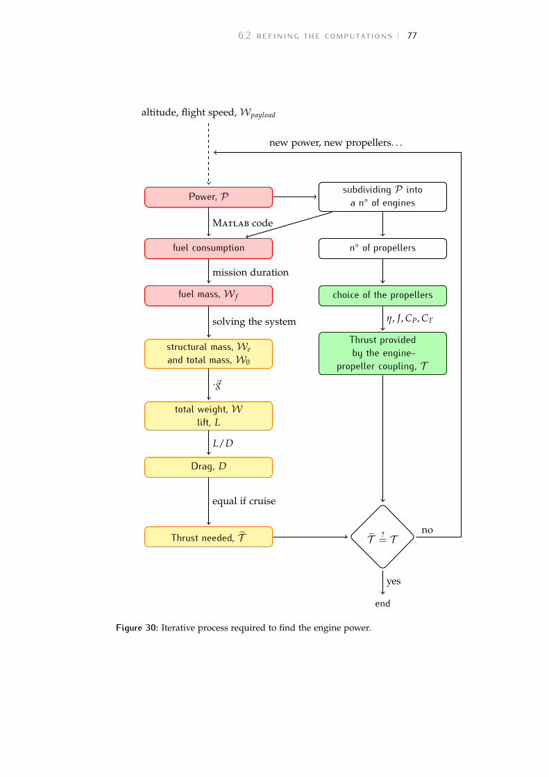
6.2 refining the computations 77
altitude, flight speed,Wpayload
Power, P subdividing P intoa n° of enginesfuel consumption n° of propellersfuel mass, W f choice of the propellers
structural mass, Weand total mass, W0
Thrust providedby the engine-propeller coupling, Ttotal weight, Wlift, L
Drag, D
Thrust needed, T T ?= T
end
Matlab code
mission duration
η, J, CP, CTsolving the system
·~g
L/D
equal if cruise
yes
no
new power, new propellers. . .
Figure 30: Iterative process required to find the engine power.
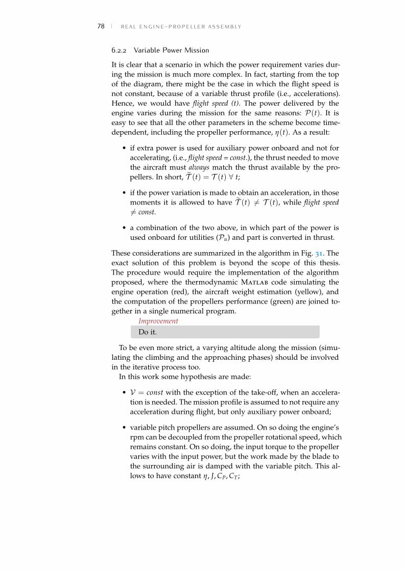
78 real engine-propeller assembly6.2.2 Variable Power MissionIt is clear that a scenario in which the power requirement varies dur-ing the mission is much more complex. In fact, starting from the topof the diagram, there might be the case in which the flight speed isnot constant, because of a variable thrust profile (i.e., accelerations).Hence, we would have flight speed (t). The power delivered by theengine varies during the mission for the same reasons: P(t). It iseasy to see that all the other parameters in the scheme become time-dependent, including the propeller performance, η(t). As a result:
• if extra power is used for auxiliary power onboard and not foraccelerating, (i.e., flight speed = const.), the thrust needed to movethe aircraft must always match the thrust available by the pro-pellers. In short, T (t) = T (t) ∀ t;
• if the power variation is made to obtain an acceleration, in thosemoments it is allowed to have T (t) 6= T (t), while flight speed6= const.
• a combination of the two above, in which part of the power isused onboard for utilities (Pu) and part is converted in thrust.
These considerations are summarized in the algorithm in Fig. 31. Theexact solution of this problem is beyond the scope of this thesis.The procedure would require the implementation of the algorithmproposed, where the thermodynamic Matlab code simulating theengine operation (red), the aircraft weight estimation (yellow), andthe computation of the propellers performance (green) are joined to-gether in a single numerical program.
ImprovementDo it.
To be even more strict, a varying altitude along the mission (simu-lating the climbing and the approaching phases) should be involvedin the iterative process too.
In this work some hypothesis are made:
• V = const with the exception of the take-off, when an accelera-tion is needed. The mission profile is assumed to not require anyacceleration during flight, but only auxiliary power onboard;
• variable pitch propellers are assumed. On so doing the engine’srpm can be decoupled from the propeller rotational speed, whichremains constant. On so doing, the input torque to the propellervaries with the input power, but the work made by the blade tothe surrounding air is damped with the variable pitch. This al-lows to have constant η, J, CP, CT;
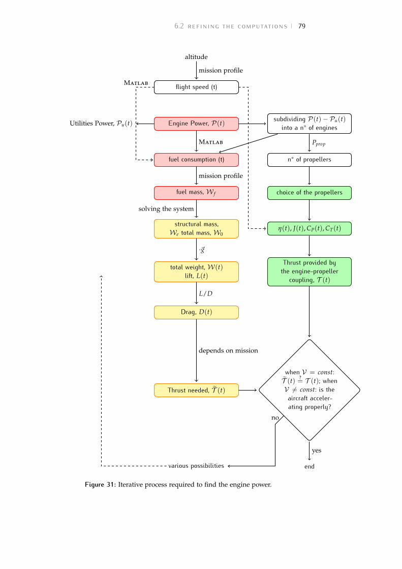
6.2 refining the computations 79altitude
flight speed (t)
Utilities Power, Pu(t) Engine Power, P(t) subdividing P(t)− Pu(t)into a n° of enginesfuel consumption (t) n° of propellers
fuel mass, W f choice of the propellersstructural mass,We total mass, W0
η(t), J(t), CP(t), CT(t)
total weight, W(t)lift, L(t)
Thrust provided bythe engine-propellercoupling, T (t)Drag, D(t)
Thrust needed, T (t)when V = const:T (t) ?
= T (t); whenV 6= const: is theaircraft acceler-ating properly?
various possibilities end
mission profile
Matlab
Matlab Pprop
mission profile
solving the system
·~g
L/D
depends on mission
yes
no
Figure 31: Iterative process required to find the engine power.
80 real engine-propeller assemblyPower
0 duration[h]
+100% Pcruise
+40% Pcruise
Pcruise
1 242526 50
Figure 32: Power requirement profile for 50 hours mission.
• with respect to Section 4.4 and to the power profile in Fig. 25, amore realistic power profile is now considered (Fig. 32). There isone power peak at half mission, lasting two hours and represent-ing the duty to be accomplished at the furthest point from thebase, and one smaller power request at take-off, one hour long.
When the decision block is reached, the thrust at take-off shouldbe checked, i.e. the thrust developed by the propellers must grant theacceleration needed to reach the take-of speed. Here is the procedure:the difference between the thrust and the drag is the net force, T −D = F. The net uniform acceleration is given by a = F/W0. Hence,since the take-off velocity is fixed (see Sec. B.1), that velocity will bereached after s = VTO/a seconds.
If this duration is within a certain range, e.g. between 10 and 20 sec-onds, then the acceleration is considered acceptable, else a differentthrust must be provided.
6.3 resultsWhen convergence is reached, the aircraft engines and propellers arefully sized. The configurations obtained are tested over missions upto 50 hours. While the turbine configuration is tied to be single engine-single propeller, the Diesel configuration can be designed to be madeby two-two, three-three, and four-four of these elements. The resultsof the iterations are shown in Tab. 10. Concerning the turbine technol-ogy, a compression ratio π = 40 represents the current state of the art[2],[3]. A comparison with an advanced π = 60 is presented, show-ing the potential of investing in this technology; however, increasingπ certainly involves an increase in dimension and weight.
The propellers selected from the last iteration are reported in Table 11.The weight of each propeller is based on data sheets available in liter-ature [4]; those selected are aluminum made.
The results for the constant-cruise mission are shown in Fig. 33. Forshort durations the gas-turbine is lighter than the Diesel compounds,
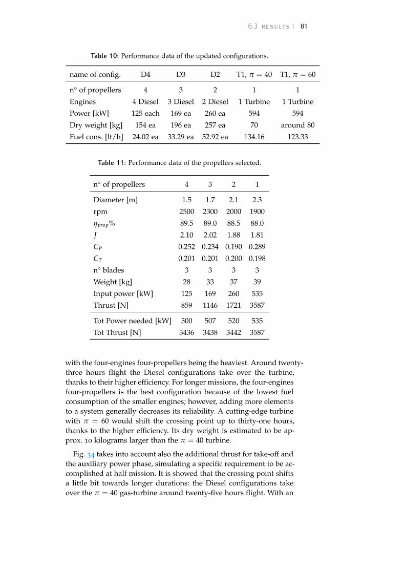
6.3 results 81Table 10: Performance data of the updated configurations.
name of config. D4 D3 D2 T1, π = 40 T1, π = 60
n° of propellers 4 3 2 1 1
Engines 4 Diesel 3 Diesel 2 Diesel 1 Turbine 1 Turbine
Power [kW] 125 each 169 ea 260 ea 594 594
Dry weight [kg] 154 ea 196 ea 257 ea 70 around 80
Fuel cons. [lt/h] 24.02 ea 33.29 ea 52.92 ea 134.16 123.33
Table 11: Performance data of the propellers selected.
n° of propellers 4 3 2 1
Diameter [m] 1.5 1.7 2.1 2.3
rpm 2500 2300 2000 1900
ηprop% 89.5 89.0 88.5 88.0
J 2.10 2.02 1.88 1.81
CP 0.252 0.234 0.190 0.289
CT 0.201 0.201 0.200 0.198
n° blades 3 3 3 3
Weight [kg] 28 33 37 39
Input power [kW] 125 169 260 535
Thrust [N] 859 1146 1721 3587
Tot Power needed [kW] 500 507 520 535
Tot Thrust [N] 3436 3438 3442 3587
with the four-engines four-propellers being the heaviest. Around twenty-three hours flight the Diesel configurations take over the turbine,thanks to their higher efficiency. For longer missions, the four-enginesfour-propellers is the best configuration because of the lowest fuelconsumption of the smaller engines; however, adding more elementsto a system generally decreases its reliability. A cutting-edge turbinewith π = 60 would shift the crossing point up to thirty-one hours,thanks to the higher efficiency. Its dry weight is estimated to be ap-prox. 10 kilograms larger than the π = 40 turbine.
Fig. 34 takes into account also the additional thrust for take-off andthe auxiliary power phase, simulating a specific requirement to be ac-complished at half mission. It is showed that the crossing point shiftsa little bit towards longer durations: the Diesel configurations takeover the π = 40 gas-turbine around twenty-five hours flight. With an
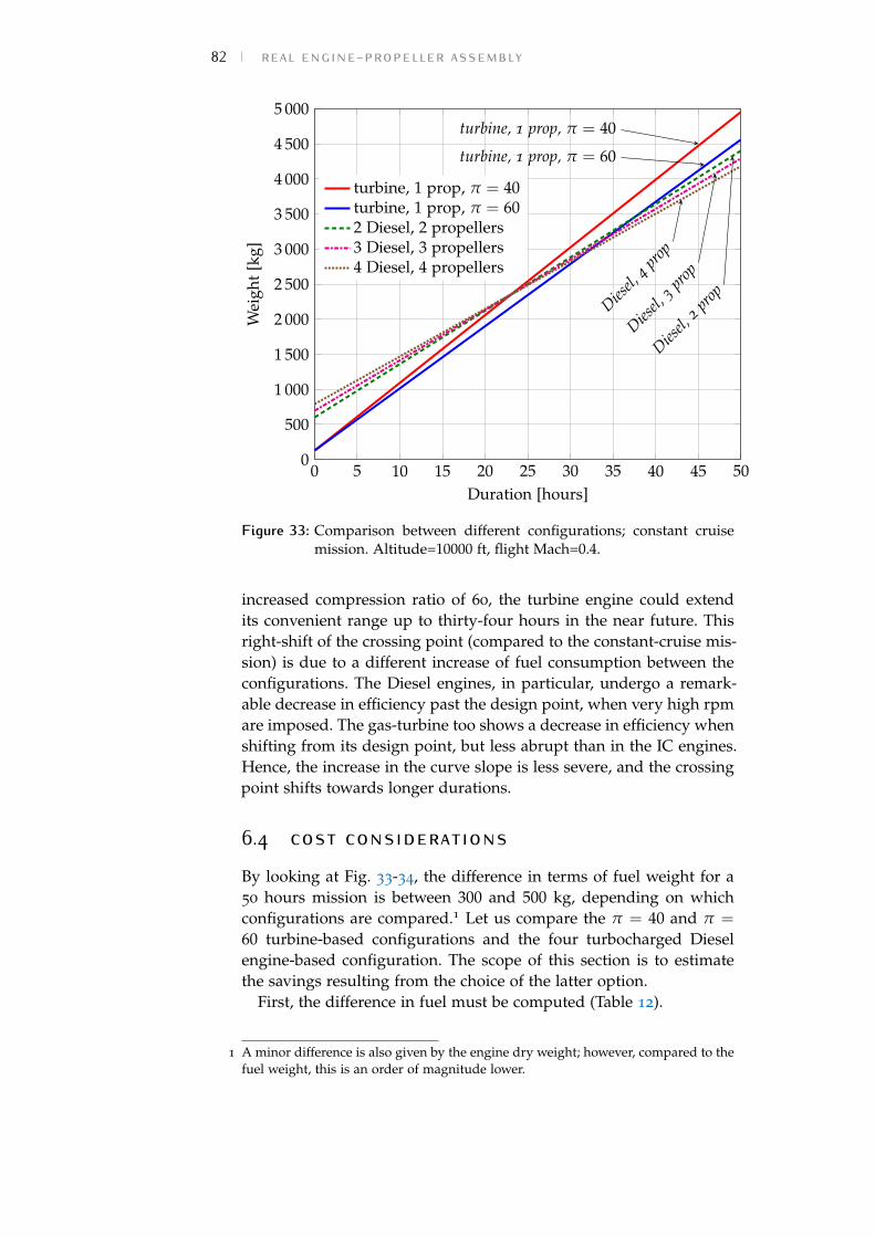
82 real engine-propeller assembly
0 5 10 15 20 25 30 35 40 45 500
500
1 000
1 500
2 000
2 500
3 000
3 500
4 000
4 500
5 000turbine, 1 prop, π = 40
turbine, 1 prop, π = 60
Diesel,
2 prop
Diesel,
3 prop
Diesel,
4 prop
Duration [hours]
Wei
ght
[kg]
turbine, 1 prop, π = 40turbine, 1 prop, π = 602 Diesel, 2 propellers3 Diesel, 3 propellers4 Diesel, 4 propellers
Figure 33: Comparison between different configurations; constant cruisemission. Altitude=10000 ft, flight Mach=0.4.
increased compression ratio of 60, the turbine engine could extendits convenient range up to thirty-four hours in the near future. Thisright-shift of the crossing point (compared to the constant-cruise mis-sion) is due to a different increase of fuel consumption between theconfigurations. The Diesel engines, in particular, undergo a remark-able decrease in efficiency past the design point, when very high rpmare imposed. The gas-turbine too shows a decrease in efficiency whenshifting from its design point, but less abrupt than in the IC engines.Hence, the increase in the curve slope is less severe, and the crossingpoint shifts towards longer durations.
6.4 cost considerationsBy looking at Fig. 33-34, the difference in terms of fuel weight for a50 hours mission is between 300 and 500 kg, depending on whichconfigurations are compared.1 Let us compare the π = 40 and π =
60 turbine-based configurations and the four turbocharged Dieselengine-based configuration. The scope of this section is to estimatethe savings resulting from the choice of the latter option.
First, the difference in fuel must be computed (Table 12).
1 A minor difference is also given by the engine dry weight; however, compared to thefuel weight, this is an order of magnitude lower.
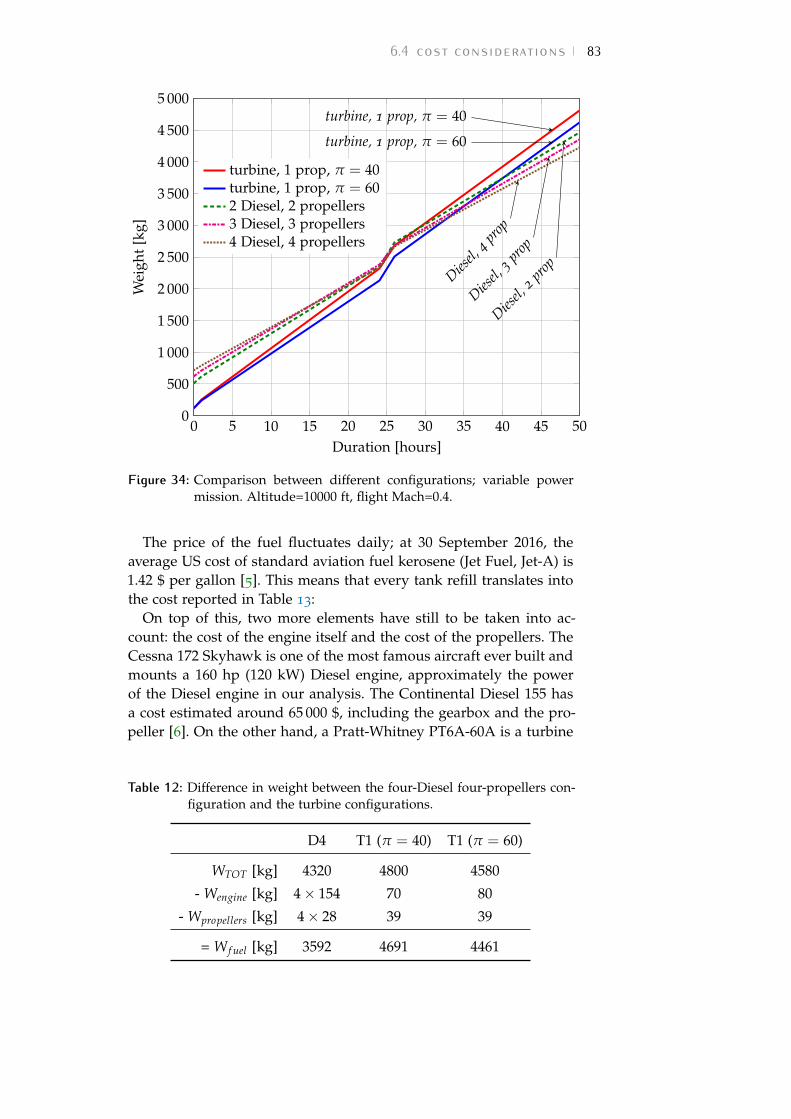
6.4 cost considerations 83
0 5 10 15 20 25 30 35 40 45 500
500
1 000
1 500
2 000
2 500
3 000
3 500
4 000
4 500
5 000turbine, 1 prop, π = 40
turbine, 1 prop, π = 60
Diesel,
2 prop
Diesel,
3 prop
Diesel,
4 prop
Duration [hours]
Wei
ght
[kg]
turbine, 1 prop, π = 40turbine, 1 prop, π = 602 Diesel, 2 propellers3 Diesel, 3 propellers4 Diesel, 4 propellers
Figure 34: Comparison between different configurations; variable powermission. Altitude=10000 ft, flight Mach=0.4.
The price of the fuel fluctuates daily; at 30 September 2016, theaverage US cost of standard aviation fuel kerosene (Jet Fuel, Jet-A) is1.42 $ per gallon [5]. This means that every tank refill translates intothe cost reported in Table 13:
On top of this, two more elements have still to be taken into ac-count: the cost of the engine itself and the cost of the propellers. TheCessna 172 Skyhawk is one of the most famous aircraft ever built andmounts a 160 hp (120 kW) Diesel engine, approximately the powerof the Diesel engine in our analysis. The Continental Diesel 155 hasa cost estimated around 65 000 $, including the gearbox and the pro-peller [6]. On the other hand, a Pratt-Whitney PT6A-60A is a turbine
Table 12: Difference in weight between the four-Diesel four-propellers con-figuration and the turbine configurations.
D4 T1 (π = 40) T1 (π = 60)
WTOT [kg] 4320 4800 4580
- Wengine [kg] 4× 154 70 80
- Wpropellers [kg] 4× 28 39 39
= W f uel [kg] 3592 4691 4461
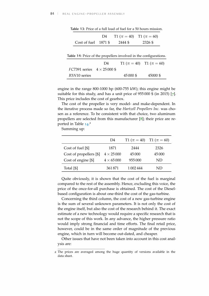
84 real engine-propeller assemblyTable 13: Price of a full load of fuel for a 50 hours mission.
D4 T1 (π = 40) T1 (π = 60)
Cost of fuel 1871 $ 2444 $ 2326 $
Table 14: Price of the propellers involved in the configurations.
D4 T1 (π = 40) T1 (π = 60)
FC7391 series 4× 25 000 $
B3N10 series 45 000 $ 45000 $
engine in the range 800-1000 hp (600-755 kW); this engine might besuitable for this study, and has a unit price of 955 000 $ (in 2015) [7].This price includes the cost of gearbox.
The cost of the propeller is very model- and make-dependent. Inthe iterative process made so far, the Hartzell Propellers Inc. was cho-sen as a reference. To be consistent with that choice, two aluminumpropellers are selected from this manufacturer [8]; their price are re-ported in Table 14.2
Summing up:
D4 T1 (π = 40) T1 (π = 60)
Cost of fuel [$] 1871 2444 2326
Cost of propellers [$] 4× 25 000 45 000 45 000
Cost of engine [$] 4× 65 000 955 000 ND
Total [$] 361 871 1 002 444 ND
Quite obviously, it is shown that the cost of the fuel is marginalcompared to the rest of the assembly. Hence, excluding this voice, theprice of the once-for-all purchase is obtained. The cost of the Diesel-based configuration is about one-third the cost of the gas-turbine.
Concerning the third column, the cost of a new gas-turbine engineis the sum of several unknown parameters. It is not only the cost ofthe engine itself, but also the cost of the research behind it. The exactestimate of a new technology would require a specific research that isnot the scope of this work. In any advance, the higher pressure ratiowould imply strong financial and time efforts. The final retail price,however, could be in the same order of magnitude of the previousengine, which in turn will become out-dated, and cheaper.
Other issues that have not been taken into account in this cost anal-ysis are:
2 The prices are averaged among the huge quantity of versions available in thedata sheet.
References 85• maintenance costs: overhaul, replacing of parts, inspections;
• cost of certifications and approvals;
• installation and delivery costs.
The choice of four Diesel engines implies four times the cost ofone inspection (and repairing); also, the probability of a failure isfour times increased. Many problems still plague these engines andespecially the problem with reliability, low Time Between Overhaul(TBO) or Time Between Replacement (TBR), maintenance availabilityand cost [9]. The choice of the turbine instead of the Diesel engine,indeed, is based on reliability issues too, since the turbine technologyhas a lower shutdown rate per hour of flight. Finally, other aspects totake into account are: noise, vibrations, compactness, emission of pol-lutants, need of extremely variable power (as in aerobatic vehicles).
This section aimed to give a very general guideline about the costsof the configurations proposed, and do not expect to be exact norcomplete. Nevertheless, it points out the two main aspects concerningthe cost of each configuration: first, the 4-stroke Diesel assembly in-volves less expensive engines, and second, every long flight is cheaperbecause of the lower fuel consumption. The lower amount of fuel re-quired for a long mission implies savings for every flight made, whichmay justify the higher rate of maintenance. Moreover, a smaller andlighter tank is required, with the benefit of lower structural weightand size.
references[1] L. Piancastelli, L. Frizziero, S. Pica, and G. Donnici. “High Alti-
tude Operations with Piston Engines Power Plant Design Opti-mization, Part I: Introduction.” In: ARPN Journal of Engineeringand Apllied Sciences 11.5 (2006).
[2] CFM International. The Leap Engine. Performance. Execution. Tech-nology. Retrieved October 12, 2016. 2016. url: https://www.cfmaeroengines.com/engines/leap/.
[3] L. Piancastelli, L. Frizziero, and I. Rocchi. “Feasible OptimumDesign of a Turbocompound Diesel Brayton Cycle for Diesel-Turbo-Fan Aircraft Propulsion.” In: International Journal of Heatand Technology 30.2 (2012), pp. 121–126.
[4] Hartzell Propeller Inc. Propeller Owner’s Manual and Logbook. Ver-sion 14. Piqua, OH 45356-2634 U.S.A.
[5] International Air Transport Association (IATA). Fuel Price Analy-sis. url: http://www.iata.org/publications/economics/fuel-monitor/Pages/price-analysis.aspx.

86 real engine-propeller assembly[6] Aircraft Owners and Pilots Association (AOPA). Little Diesel,
Big Fuel Savings. url: https://www.aopa.org/news-and-media/all-news/2015/february/pilot/f_diesel.
[7] J. Kasper O. Balle (Forecast International). About the Pratt &Whitney PT6A. url: http://www.fi-powerweb.com/Engine/PW-CANADA-PT6A.html.
[8] Hartzell Propeller Inc. 2016 Price List. Piqua, OH 45356-2634
U.S.A.
[9] N. E. Daidzic, L. Piancastelli, and A. Cattini. “Diesel engines forlight-to-medium helicopters and airplanes (Editorial).” In: Inter-national Journal of Aviation, Aeronautics, and Aerospace 1.3 (2014).url: http://commons.erau.edu/ijaaa/vol1/iss3/2.
7 C O N C L U S I O N S A N D F U T U R EW O R K7.1 conslusionsI n this work a method for choosing the best engine and layout
to drive a lightweight long-range UAV was proposed. Particularattention was given to the engine technology used, as well as thearrangement of the engines onboard and to the connections with thepropellers. A lack in literature studying the scenario between 200 and500 kW and missions beyond 20 hours was present.
Many power sources have been selected for this study. Several ex-isting engines were classified basing on their power, weight, size andfuel consumption. Comparisons among them outlined the reciprocat-ing engines and the turbine technology as the most promising. Elec-tric propulsion was discarded because of the exceeding weight of thebatteries; turbocharging was preferred to the natural aspirated coun-terpart for internal combustion engines.
Five engines were selected: 2 and 4 stroke, spark- and compression-ignition turbocharged engines, and the gas-turbine engine. A Matlab
code was written for each, simulating their thermodynamic cycle.Output properties as power, efficiency and fuel consumption wereobtained, for different levels of power and altitude. A best-fit correla-tion was developed to estimate the engines weight. Different arrange-ments of engine-propellers were proposed.
An analysis of the propeller efficiency was also made, by meansof theoretical concepts and experimental diagrams. It was outlinedthat smaller slow-rotating propellers give a better propeller efficiency.A preliminary sizing of the aircraft was performed as well. Finally,the overall system composed by structure, payload, engines and pro-pellers was optimized for a 50 hours mission, in order to obtain thehighest thermal efficiency and the lowest weight.
The thermal analysis has shown the advantages of replacing a smallgas-turbine with one or more turbocharged 4-stroke Diesel engines.Increases in efficiency and decreases in fuel consumption can result.These advantages can translate to increases in range and/or flightduration, plus a reduction in fuel tank volume and weight.
87
88 conclusions and future workThe use of multiple Diesel engines, coupled with the same number
of propellers, results in lower fuel weight for missions beyond the23-25 hours flight; if a high-performance turbine is used, the rangeis extended to 31-34 hours in the next future. The presence of theturbocharger for altitude compensation allows to keep the IC engineat its best performance over a larger flight envelope.
Replacing a gas-turbine with multiple Diesel engines presents prob-lems concerning the reliability of the system, as well as noise, vi-brations and size, which are very important requirements in a long-duration UAV. However, the use of reciprocating engines allows sav-ings for purchase, maintenance and refueling. Considerations on effi-ciency and weight have shown the non-feasibility of using mechanicalconnections between one engine and multiple propellers, nor the useof electric generators to drive electric motors. The availability of moreefficient electric generators and batteries could cause reconsiderationof the hybrid and pure-electric options in the future.
7.2 suggestions for future workThe accuracy of the numerical codes has already been discussed inSec. 3.5.1. More realistic heat transfer models can be implemented,accounting for radiative and convective heat transfer through a tem-perature-variating wall. Gradual opening and closing of intake andexhaust valves should be included, also, timing should be function ofrpm, e.g. delaying the inlet valve closing for enhancing the cylinderscavenging at high rpm. More refined combustion models could be in-cluded in the cycle; experiments should be performed to simulate thereal heat release curve for the Diesel combustion model. Modeling theturbocharger operation by translating maps into functions could beconsidered, synchronizing its capabilities within the rest of the code.Finally, the accuracy of the numerical codes should be compared withreal engines and/or CFD simulations in a more strict fashion.
Concerning the flight simulations, more realistic missions could beconsidered, e.g. accounting for altitude variation during the mission.Moreover, the power of the engine should consider the decrease ofthe aircraft weight during the mission due to the fuel consumption.It should be given a try to include these variations into an algorithmable to compute the aircraft weight at every instant.
A more detailed cost analysis should be performed if needed, in-cluding an estimate of maintenance costs and mean time to failure;include issues that possibly drive the choice of a certain technol-ogy, as size, vibrations and noise. Further improvements in IC en-gines efficiency and weight include different arrangements of the tur-bochargers: it is conceivable to save weight and volume if a singleturbocharger could supply air to multiple engines simultaneously.

Part III
A P P E N D I X

A E N G I N E S R E V I E WI n this chapter a collection of engines in presented. This is the
product of a deep research through several data sheets. All theengines presented are or have been on the market, i.e. no prototypeshave been considered.
The engines are classified according to their power, fuel consump-tion and size. Unfortunately, turbojet and turbofan engines are com-monly rated with their thrust, instead of power. In order to make com-parisons, the power of each engine must be computed. The followingprocedure is applied, according to [1]. By assuming the aircraft asa black box, with mair and m f entering and (mair + m f ) exiting theboundaries, with a perfectly adapted nozzle, the following relationsare derived:
T = (mair + m f )Vjet − mairV
∆KE =12
[(mair + m f )V2
jet − mairV2]
P = VT = V[(mair + m f )Vjet − mairV
]TSFC =
m f
T
(127)
where T is the net thrust, ∆KE is the rate of change of kinetic energy,P is the power associated with propelling the aircraft, and TSFC isthe thrust specific fuel consumption.
The above 4 equations contain 5 unknowns: m f ,V ,Vjet, ∆KE,P . Theother terms as T, mair, TSFC should be given from data sheets.
If T is the static thrust at sea level, V = 0 in this condition and thethird equation drops. Hence, the remaining system of 3 equations in3 unknowns (m f ,Vjet, ∆KE) can be solved.
T = (mair + m f )Vjet
∆KE =12
[(mair + m f )V2
jet
]TSFC =
m f
T
(128)
Else, if one of the information is missing (because confidential), orif the thrust is not the static one, the previous simplification can notbe done; another information should be given, e.g. V . or m f . Turbofan
91
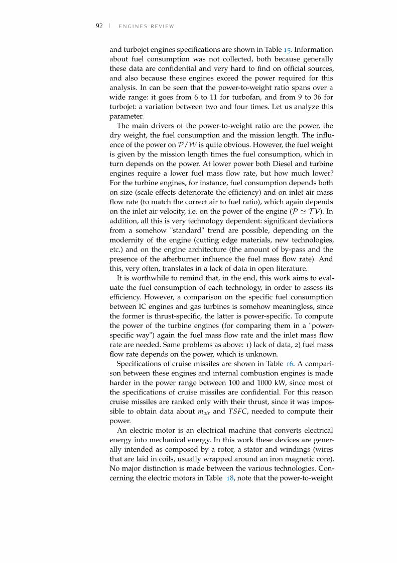
92 engines reviewand turbojet engines specifications are shown in Table 15. Informationabout fuel consumption was not collected, both because generallythese data are confidential and very hard to find on official sources,and also because these engines exceed the power required for thisanalysis. In can be seen that the power-to-weight ratio spans over awide range: it goes from 6 to 11 for turbofan, and from 9 to 36 forturbojet: a variation between two and four times. Let us analyze thisparameter.
The main drivers of the power-to-weight ratio are the power, thedry weight, the fuel consumption and the mission length. The influ-ence of the power on P/W is quite obvious. However, the fuel weightis given by the mission length times the fuel consumption, which inturn depends on the power. At lower power both Diesel and turbineengines require a lower fuel mass flow rate, but how much lower?For the turbine engines, for instance, fuel consumption depends bothon size (scale effects deteriorate the efficiency) and on inlet air massflow rate (to match the correct air to fuel ratio), which again dependson the inlet air velocity, i.e. on the power of the engine (P ' T V). Inaddition, all this is very technology dependent: significant deviationsfrom a somehow "standard" trend are possible, depending on themodernity of the engine (cutting edge materials, new technologies,etc.) and on the engine architecture (the amount of by-pass and thepresence of the afterburner influence the fuel mass flow rate). Andthis, very often, translates in a lack of data in open literature.
It is worthwhile to remind that, in the end, this work aims to eval-uate the fuel consumption of each technology, in order to assess itsefficiency. However, a comparison on the specific fuel consumptionbetween IC engines and gas turbines is somehow meaningless, sincethe former is thrust-specific, the latter is power-specific. To computethe power of the turbine engines (for comparing them in a "power-specific way") again the fuel mass flow rate and the inlet mass flowrate are needed. Same problems as above: 1) lack of data, 2) fuel massflow rate depends on the power, which is unknown.
Specifications of cruise missiles are shown in Table 16. A compari-son between these engines and internal combustion engines is madeharder in the power range between 100 and 1000 kW, since most ofthe specifications of cruise missiles are confidential. For this reasoncruise missiles are ranked only with their thrust, since it was impos-sible to obtain data about mair and TSFC, needed to compute theirpower.
An electric motor is an electrical machine that converts electricalenergy into mechanical energy. In this work these devices are gener-ally intended as composed by a rotor, a stator and windings (wiresthat are laid in coils, usually wrapped around an iron magnetic core).No major distinction is made between the various technologies. Con-cerning the electric motors in Table 18, note that the power-to-weight
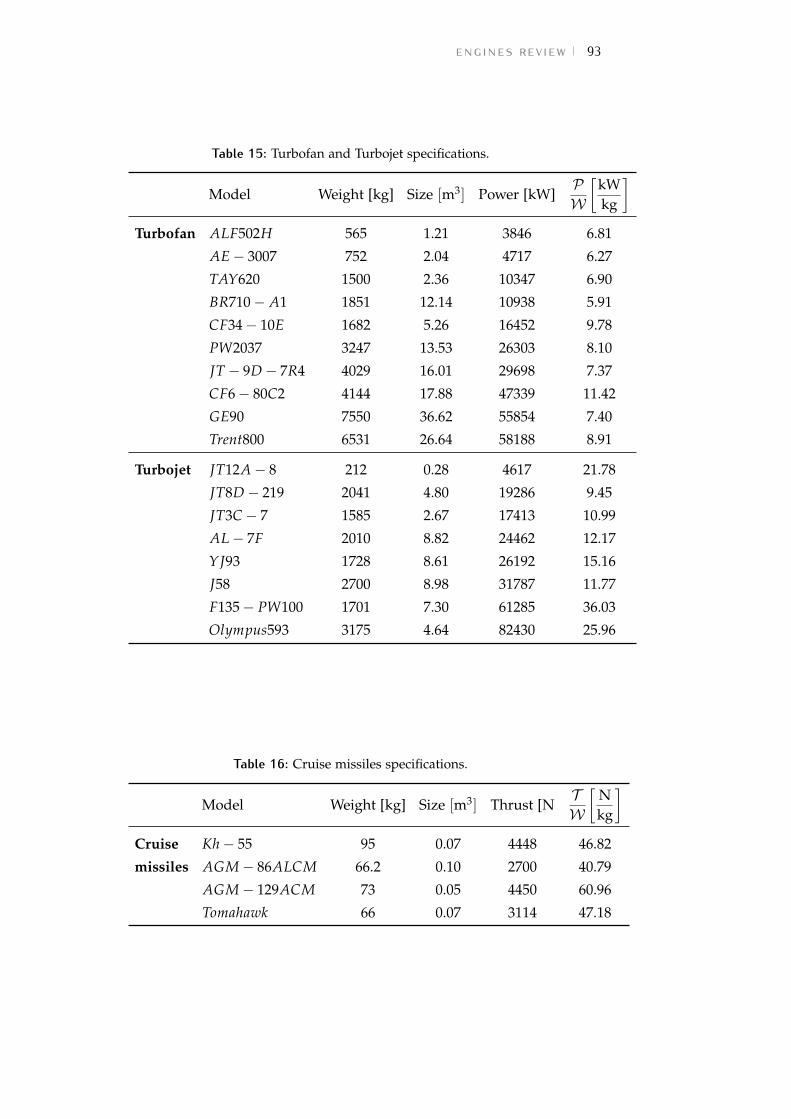
engines review 93
Table 15: Turbofan and Turbojet specifications.
Model Weight [kg] Size [m3] Power [kW]PW
[kWkg
]Turbofan ALF502H 565 1.21 3846 6.81
AE− 3007 752 2.04 4717 6.27
TAY620 1500 2.36 10347 6.90
BR710− A1 1851 12.14 10938 5.91
CF34− 10E 1682 5.26 16452 9.78
PW2037 3247 13.53 26303 8.10
JT − 9D− 7R4 4029 16.01 29698 7.37
CF6− 80C2 4144 17.88 47339 11.42
GE90 7550 36.62 55854 7.40
Trent800 6531 26.64 58188 8.91
Turbojet JT12A− 8 212 0.28 4617 21.78
JT8D− 219 2041 4.80 19286 9.45
JT3C− 7 1585 2.67 17413 10.99
AL− 7F 2010 8.82 24462 12.17
YJ93 1728 8.61 26192 15.16
J58 2700 8.98 31787 11.77
F135− PW100 1701 7.30 61285 36.03
Olympus593 3175 4.64 82430 25.96
Table 16: Cruise missiles specifications.
Model Weight [kg] Size [m3] Thrust [NTW
[Nkg
]Cruise Kh− 55 95 0.07 4448 46.82
missiles AGM− 86ALCM 66.2 0.10 2700 40.79
AGM− 129ACM 73 0.05 4450 60.96
Tomahawk 66 0.07 3114 47.18
94 engines reviewratio differs of at least one order of magnitude between the enginealone and when it is coupled with batteries.
In Tables 19 and 20 each reciprocating engine is classified alongwith the number of strokes (two or four) and the ignition technique(spark or compression). Pay attention to the fact that the last six ele-ments of Table 20 are actually Formula 1 engines. This is the reasonfor their remarkable high Power-to-Weight ratio.
Finally, some specifications involving the electric generators inves-tigated are shown in Table 22. These devices are commonly producedin two types: one is a massive machine including a reciprocating en-gine. The crankshaft is mechanically linked with the generator itself;often the rpm matching is obtained trough the use of a gearbox. Thesedevices are very large and heavy, definitely not suitable for aeronauticpurposes, but quite common as assistance power source in industrialapplications. The other type does not include the engine, and arecommonly called alternators. Hence these machines are smaller andportable. In fact, the power is taken from a power source, such asan IC engine, by the use of a PTO, or Power Take Off. It is a systemcomprising a splined output shaft on a tractor or truck, which can beeasily connected and disconnected to the generator side.
references[1] N. Cumpsty. Jet Propulsion: A Simple Guide to the Aerodynamic
and Thermodynamic Design and Performance of Jet Engines. Cam-bridge University Press, 1997.
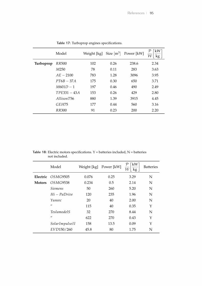
References 95
Table 17: Turboprop engines specifications.
Model Weight [kg] Size [m3] Power [kW]PW
[kWkg
]Turboprop RR500 102 0.26 238.6 2.34
M250 78 0.11 283 3.63
AE− 2100 783 1.28 3096 3.95
PT6B− 37A 175 0.30 650 3.71
M601D− 1 197 0.46 490 2.49
TPE331− 43A 153 0.26 429 2.80
AllisonT56 880 1.39 3915 4.45
GEH75 177 0.44 560 3.16
RR300 91 0.23 200 2.20
Table 18: Electric motors specifications. Y = batteries included, N = batteriesnot included.
Model Weight [kg] Power [kW]PW
[kWkg
]Batteries
Electric OSMG9505 0.076 0.25 3.29 N
Motors OSMG9538 0.234 0.5 2.14 N
Siemens 50 260 5.20 N
Hi− PaDrive 120 235 1.96 N
Yuneec 20 40 2.00 N
” 115 40 0.35 Y
TeslamodelS 32 270 8.44 N
” 622 270 0.43 Y
SolarImpulseI I 158 13.5 0.09 Y
EVD150/260 45.8 80 1.75 N
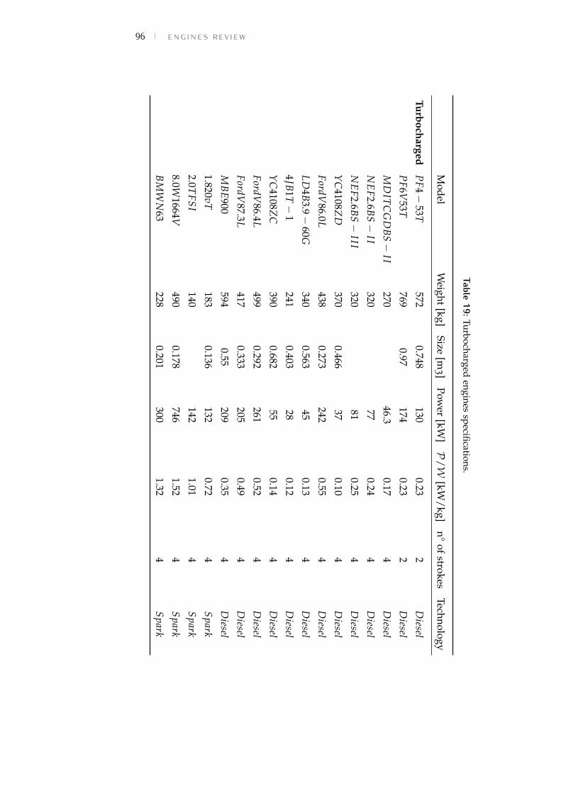
96 engines review
Table19:Turbocharged
enginesspecifications.
Model
Weight
[kg]Size
[m3]
Power
[kW]P
/W[kW
/kg]n°
ofstrokes
Technology
TurbochargedP
F4−53T
5720.748
1300.23
2D
iesel
PF6V
53T769
0.97174
0.232
Diesel
MD
ITC
GD
BS−
II270
46.30.17
4D
iesel
NE
F2.6BS−
II320
770.24
4D
iesel
NE
F2.6BS−
III320
810.25
4D
iesel
YC
4108ZD
3700.466
370.10
4D
iesel
FordV86.0L
4380.273
2420.55
4D
iesel
LD4B
3.9−60G
3400.563
450.13
4D
iesel
4JB1T−
1241
0.40328
0.124
Diesel
YC
4108ZC
3900.682
550.14
4D
iesel
FordV86.4L
4990.292
2610.52
4D
iesel
FordV87.3L
4170.333
2050.49
4D
iesel
MB
E900
5940.55
2090.35
4D
iesel
1.820vT183
0.136132
0.724
Spark
2.0TFS
I140
1421.01
4S
park
8.0W1664V
4900.178
7461.52
4S
park
BM
WN
63228
0.201300
1.324
Spark
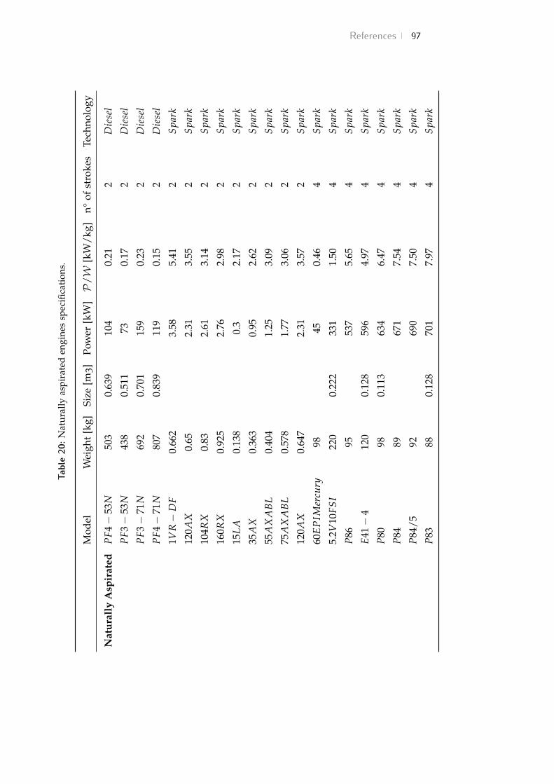
References 97Ta
ble
20:N
atur
ally
aspi
rate
den
gine
ssp
ecifi
cati
ons.
Mod
elW
eigh
t[k
g]Si
ze[m
3]
Pow
er[k
W]P
/W
[kW
/kg]
n°of
stro
kes
Tech
nolo
gy
Nat
ural
lyA
spir
ated
PF4−
53N
503
0.63
910
40.
212
Die
sel
PF3−
53N
438
0.51
173
0.17
2D
iese
l
PF3−
71N
692
0.70
115
90.
232
Die
sel
PF4−
71N
807
0.83
911
90.
152
Die
sel
1VR−
DF
0.66
23.
585.
412
Spa
rk
120A
X0.
652.
313.
552
Spa
rk
104R
X0.
832.
613.
142
Spa
rk
160R
X0.
925
2.76
2.98
2S
park
15L
A0.
138
0.3
2.17
2S
park
35A
X0.
363
0.95
2.62
2S
park
55A
XA
BL
0.40
41.
253.
092
Spa
rk
75A
XA
BL
0.57
81.
773.
062
Spa
rk
120A
X0.
647
2.31
3.57
2S
park
60E
PIM
ercu
ry98
450.
464
Spa
rk
5.2V
10FS
I22
00.
222
331
1.50
4S
park
P86
9553
75.
654
Spa
rk
E41−
412
00.
128
596
4.97
4S
park
P80
980.
113
634
6.47
4S
park
P84
8967
17.
544
Spa
rk
P84
/5
9269
07.
504
Spa
rk
P83
880.
128
701
7.97
4S
park
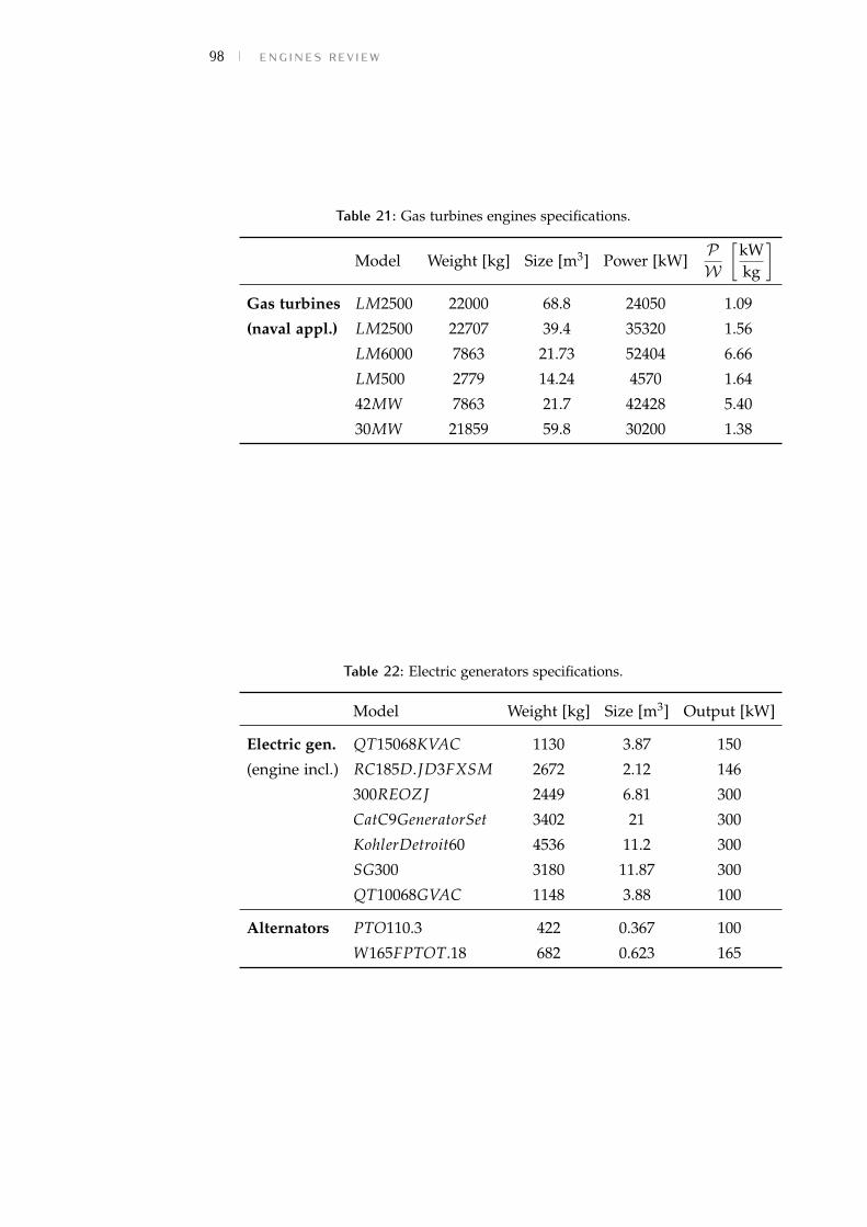
98 engines review
Table 21: Gas turbines engines specifications.
Model Weight [kg] Size [m3] Power [kW]PW
[kWkg
]Gas turbines LM2500 22000 68.8 24050 1.09
(naval appl.) LM2500 22707 39.4 35320 1.56
LM6000 7863 21.73 52404 6.66
LM500 2779 14.24 4570 1.64
42MW 7863 21.7 42428 5.40
30MW 21859 59.8 30200 1.38
Table 22: Electric generators specifications.
Model Weight [kg] Size [m3] Output [kW]
Electric gen. QT15068KVAC 1130 3.87 150
(engine incl.) RC185D.JD3FXSM 2672 2.12 146
300REOZJ 2449 6.81 300
CatC9GeneratorSet 3402 21 300
KohlerDetroit60 4536 11.2 300
SG300 3180 11.87 300
QT10068GVAC 1148 3.88 100
Alternators PTO110.3 422 0.367 100
W165FPTOT.18 682 0.623 165
B VA R I A B L E P O W E R P R O F I L ESection 4.4 introduced the concept of variable power requirement.The profile of Fig. 25 and the correspondent power increments arejustified by the following analysis.
b.1 take-off phaseThe analysis of this section is focusing on relating the engine’s powerwith the useful thrust and the aircraft speed. Both these parametersare important in defining the take-off phase. In fact, we need to knowwhether a certain power increment (say, +40%) is able to guaranteeenough thrust and velocity for taking off.
In aeronautics, P , T , and V are linked by the so called propellerefficiency ([1], pag. 351):
ηprop =T VP . (129)
A propeller efficiency equal to 1 is now assumed for simplicity, butthe real value can be computed in advanced phases of the design, asexplained in Sec. 5. At cruise conditions:
• P = 300 kW
• M = 0.4 =⇒ V = M·c(z) ' 125 m/s
Hence, Tcruise ' 2400 N. In order to know the power at the take-off,both TTO and VTO must be estimated.
TTO A reasonable approximation suggested by [2] is that the cruisethrust (in lbf) as a function of take-off thrust is given by
Tcruise = 14300 sin(
π TTO
200000
)(130)
which can be solved for TTO. This correlation relates the perfor-mance of 26 large turbofan engines as reported in Svoboda [3].Being the aircraft in this analysis orders of magnitude smallerthan the ones studied by Svoboda, Eq. 130 tends to overestimatethe value of TTO. Alternatively, a simpler correlation developedby Svoboda himself suggests that
Tcruise = 200 + 0.2·TTO (131)
99
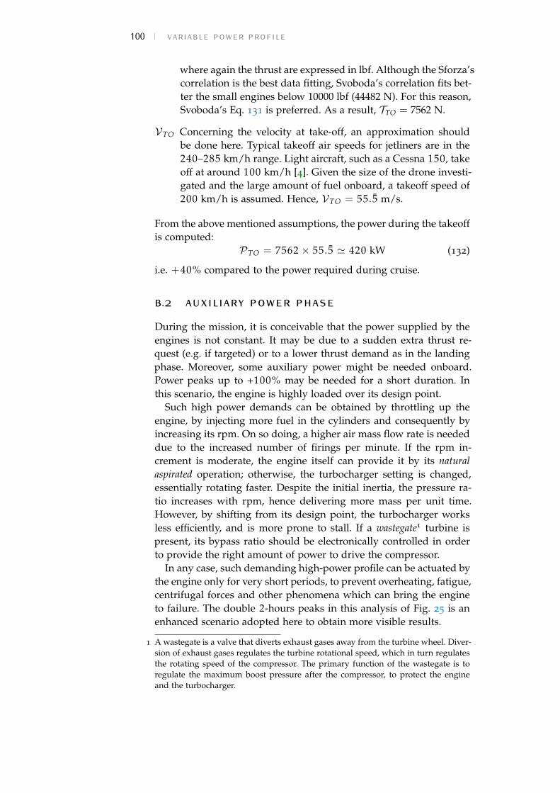
100 variable power profilewhere again the thrust are expressed in lbf. Although the Sforza’scorrelation is the best data fitting, Svoboda’s correlation fits bet-ter the small engines below 10000 lbf (44482 N). For this reason,Svoboda’s Eq. 131 is preferred. As a result, TTO = 7562 N.
VTO Concerning the velocity at take-off, an approximation shouldbe done here. Typical takeoff air speeds for jetliners are in the240–285 km/h range. Light aircraft, such as a Cessna 150, takeoff at around 100 km/h [4]. Given the size of the drone investi-gated and the large amount of fuel onboard, a takeoff speed of200 km/h is assumed. Hence, VTO = 55.5 m/s.
From the above mentioned assumptions, the power during the takeoffis computed:
PTO = 7562 × 55.5 ' 420 kW (132)
i.e. +40% compared to the power required during cruise.
b.2 auxiliary power phaseDuring the mission, it is conceivable that the power supplied by theengines is not constant. It may be due to a sudden extra thrust re-quest (e.g. if targeted) or to a lower thrust demand as in the landingphase. Moreover, some auxiliary power might be needed onboard.Power peaks up to +100% may be needed for a short duration. Inthis scenario, the engine is highly loaded over its design point.
Such high power demands can be obtained by throttling up theengine, by injecting more fuel in the cylinders and consequently byincreasing its rpm. On so doing, a higher air mass flow rate is neededdue to the increased number of firings per minute. If the rpm in-crement is moderate, the engine itself can provide it by its naturalaspirated operation; otherwise, the turbocharger setting is changed,essentially rotating faster. Despite the initial inertia, the pressure ra-tio increases with rpm, hence delivering more mass per unit time.However, by shifting from its design point, the turbocharger worksless efficiently, and is more prone to stall. If a wastegate1 turbine ispresent, its bypass ratio should be electronically controlled in orderto provide the right amount of power to drive the compressor.
In any case, such demanding high-power profile can be actuated bythe engine only for very short periods, to prevent overheating, fatigue,centrifugal forces and other phenomena which can bring the engineto failure. The double 2-hours peaks in this analysis of Fig. 25 is anenhanced scenario adopted here to obtain more visible results.
1 A wastegate is a valve that diverts exhaust gases away from the turbine wheel. Diver-sion of exhaust gases regulates the turbine rotational speed, which in turn regulatesthe rotating speed of the compressor. The primary function of the wastegate is toregulate the maximum boost pressure after the compressor, to protect the engineand the turbocharger.

References 101references[1] B. W. McCormick. Aerodynamics, Aeronautics, and Flight Mechan-
ics. 2nd ed. Wiley, 1994. isbn: 0471575062,9780471575061.
[2] Sforza P. M. Theory of Aerospace Propulsion. 2nd ed. pag. 397.Butterworth-Heinemann, 2016.
[3] Svoboda C. “Turbofan Engine Database as a Preliminary De-sign Tool.” In: Aircraft Design 3 (2000), pp. 17–31.
[4] Scott J. Airliner Takeoff Speeds. url: http://www.aerospaceweb.org/question/performance/q0088.shtml.

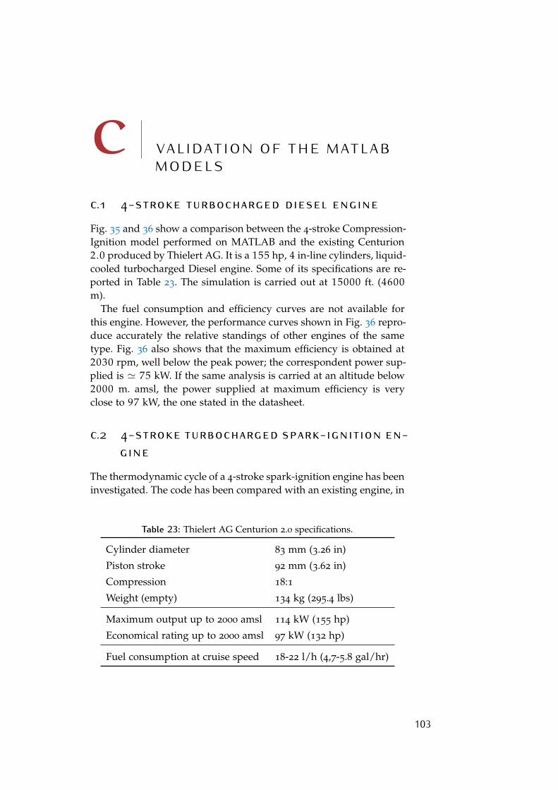
C VA L I DAT I O N O F T H E M AT L A BM O D E L Sc.1 4-stroke turbocharged diesel engineFig. 35 and 36 show a comparison between the 4-stroke Compression-Ignition model performed on MATLAB and the existing Centurion2.0 produced by Thielert AG. It is a 155 hp, 4 in-line cylinders, liquid-cooled turbocharged Diesel engine. Some of its specifications are re-ported in Table 23. The simulation is carried out at 15000 ft. (4600m).
The fuel consumption and efficiency curves are not available forthis engine. However, the performance curves shown in Fig. 36 repro-duce accurately the relative standings of other engines of the sametype. Fig. 36 also shows that the maximum efficiency is obtained at2030 rpm, well below the peak power; the correspondent power sup-plied is ' 75 kW. If the same analysis is carried at an altitude below2000 m. amsl, the power supplied at maximum efficiency is veryclose to 97 kW, the one stated in the datasheet.
c.2 4-stroke turbocharged spark-ignition en-gineThe thermodynamic cycle of a 4-stroke spark-ignition engine has beeninvestigated. The code has been compared with an existing engine, in
Table 23: Thielert AG Centurion 2.0 specifications.
Cylinder diameter 83 mm (3.26 in)
Piston stroke 92 mm (3.62 in)
Compression 18:1
Weight (empty) 134 kg (295.4 lbs)
Maximum output up to 2000 amsl 114 kW (155 hp)
Economical rating up to 2000 amsl 97 kW (132 hp)
Fuel consumption at cruise speed 18-22 l/h (4,7-5.8 gal/hr)
103
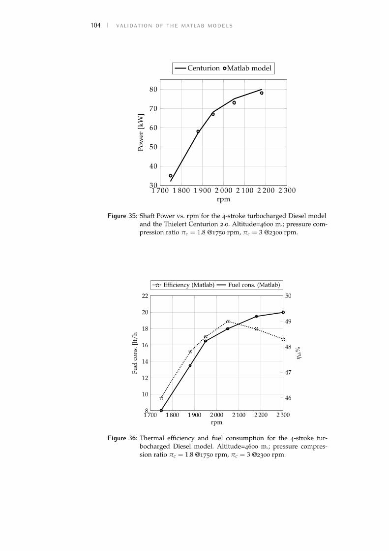
104 validation of the matlab models
1 700 1 800 1 900 2 000 2 100 2 200 2 30030
40
50
60
70
80
rpm
Pow
er[k
W]
Weight vs. PowerCenturion Matlab model
Figure 35: Shaft Power vs. rpm for the 4-stroke turbocharged Diesel modeland the Thielert Centurion 2.0. Altitude=4600 m.; pressure com-pression ratio πc = 1.8 @1750 rpm, πc = 3 @2300 rpm.
1 700 1 800 1 900 2 000 2 100 2 200 2 3008
10
12
14
16
18
20
22
rpm
Fuel
cons
.[lt
/h
46
47
48
49
50η
th%
Efficiency (Matlab) Fuel cons. (Matlab)
Figure 36: Thermal efficiency and fuel consumption for the 4-stroke tur-bocharged Diesel model. Altitude=4600 m.; pressure compres-sion ratio πc = 1.8 @1750 rpm, πc = 3 @2300 rpm.
C.3 2-stroke turbocharged spark-ignition engine 105Table 24: Rotax 914UL specifications.
Cylinder diameter 79.5 mm (3.13 in)
Piston stroke 61 mm (2.4 in)
Compression 9:1
Weight (empty) 64 kg (140.8 lbs)
Maximum Power output 84.5 kW
Maximum Torque output 144 Nm
Max revolutions 5800 rpm
3 000 3 500 4 000 4 500 5 000 5 500 6 00030
40
50
60
70
80
rpm
Pow
er[k
W]
Weight vs. PowerRotax 914 Matlab model
Figure 37: Shaft Power vs. rpm for the 4-stroke turbocharged spark-ignitionmodel and the Rotax 914. Altitude=2000 m.
order to test its accuracy. The engine chosen for the analysis is theRotax 914UL, whose specifications are reported in Table 24. For thiscomparison both the power curve (Fig. 37) and the fuel consumptioncurve (Fig. 38) are available. Hence, a more accurate comparison ispossible between the numerical code and the experimental data fromthe maker. Although with no direct comparison, the efficiency curvein Fig. 38 follows the typical non-monotonic shape.
c.3 2-stroke turbocharged spark-ignition en-gineThe engine chosen for the comparison is the Hirth 3003. The reasonof this choice is the availability of its datasheet and its power-rpm,
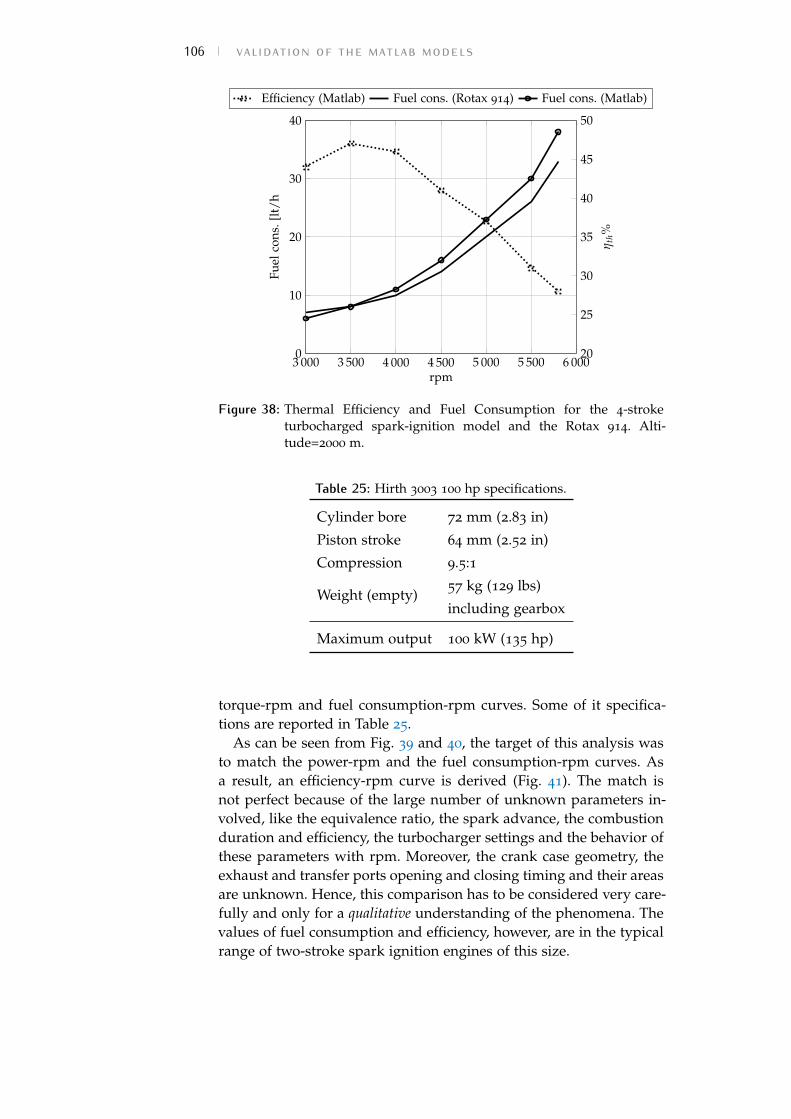
106 validation of the matlab models
3 000 3 500 4 000 4 500 5 000 5 500 6 0000
10
20
30
40
rpm
Fuel
cons
.[lt
/h
20
25
30
35
40
45
50
ηth
%
Efficiency (Matlab) Fuel cons. (Rotax 914) Fuel cons. (Matlab)
Figure 38: Thermal Efficiency and Fuel Consumption for the 4-stroketurbocharged spark-ignition model and the Rotax 914. Alti-tude=2000 m.
Table 25: Hirth 3003 100 hp specifications.
Cylinder bore 72 mm (2.83 in)
Piston stroke 64 mm (2.52 in)
Compression 9.5:1
Weight (empty)57 kg (129 lbs)
including gearbox
Maximum output 100 kW (135 hp)
torque-rpm and fuel consumption-rpm curves. Some of it specifica-tions are reported in Table 25.
As can be seen from Fig. 39 and 40, the target of this analysis wasto match the power-rpm and the fuel consumption-rpm curves. Asa result, an efficiency-rpm curve is derived (Fig. 41). The match isnot perfect because of the large number of unknown parameters in-volved, like the equivalence ratio, the spark advance, the combustionduration and efficiency, the turbocharger settings and the behavior ofthese parameters with rpm. Moreover, the crank case geometry, theexhaust and transfer ports opening and closing timing and their areasare unknown. Hence, this comparison has to be considered very care-fully and only for a qualitative understanding of the phenomena. Thevalues of fuel consumption and efficiency, however, are in the typicalrange of two-stroke spark ignition engines of this size.
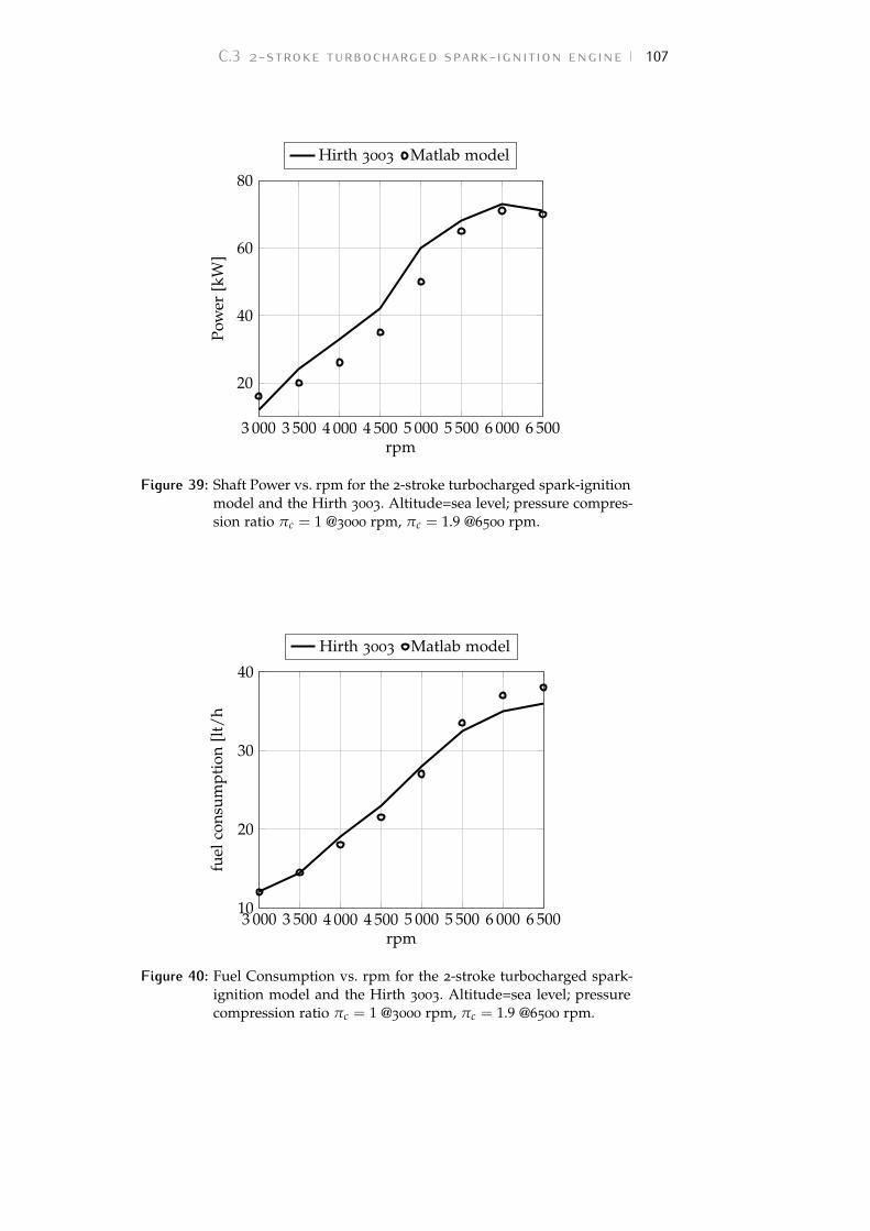
C.3 2-stroke turbocharged spark-ignition engine 107
3 000 3 500 4 000 4 500 5 000 5 500 6 000 6 500
20
40
60
80
rpm
Pow
er[k
W]
Hirth 3003 Matlab model
Figure 39: Shaft Power vs. rpm for the 2-stroke turbocharged spark-ignitionmodel and the Hirth 3003. Altitude=sea level; pressure compres-sion ratio πc = 1 @3000 rpm, πc = 1.9 @6500 rpm.
3 000 3 500 4 000 4 500 5 000 5 500 6 000 6 50010
20
30
40
rpm
fuel
cons
umpt
ion
[lt/
h
Hirth 3003 Matlab model
Figure 40: Fuel Consumption vs. rpm for the 2-stroke turbocharged spark-ignition model and the Hirth 3003. Altitude=sea level; pressurecompression ratio πc = 1 @3000 rpm, πc = 1.9 @6500 rpm.
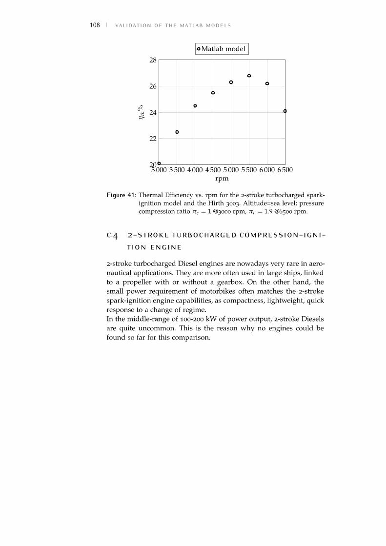
108 validation of the matlab models
3 000 3 500 4 000 4 500 5 000 5 500 6 000 6 50020
22
24
26
28
rpm
ηth
%
Matlab model
Figure 41: Thermal Efficiency vs. rpm for the 2-stroke turbocharged spark-ignition model and the Hirth 3003. Altitude=sea level; pressurecompression ratio πc = 1 @3000 rpm, πc = 1.9 @6500 rpm.
c.4 2-stroke turbocharged compression-igni-tion engine2-stroke turbocharged Diesel engines are nowadays very rare in aero-nautical applications. They are more often used in large ships, linkedto a propeller with or without a gearbox. On the other hand, thesmall power requirement of motorbikes often matches the 2-strokespark-ignition engine capabilities, as compactness, lightweight, quickresponse to a change of regime.In the middle-range of 100-200 kW of power output, 2-stroke Dieselsare quite uncommon. This is the reason why no engines could befound so far for this comparison.

colophonThis document was typeset using the typographical look-and-feelclassicthesis developed by André Miede. The style was inspiredby Robert Bringhurst’s seminal book on typography “The Elements ofTypographic Style”. classicthesis is available for both LATEX and LYX.
Final Version as of March 20, 2017 (classicthesis).