Embed Size (px)
Citation preview
Endogenous Treatment Effectsfor Count Data Models with Endogenous
Participation or Sample Selection
Massimilano Bratti & Alfonso Miranda
Institute of Education · University of London c©Bratti&Miranda (p. 1 of 27)
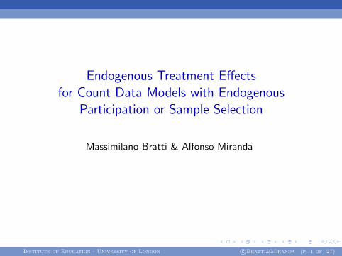
Sample selection vs ParticipationIn many fields of applied work researchers need to model a countdependent variable y that is only observed for a proportion of thesample (i.e., a sample selection problem) or that is defined only fora subset of the population (i.e., a participation problem)
Motivation Previous work The model Application Results Conclusions References
Sample selection vs ParticipationIn many fields of applied work researchers need to model a count dependentvariable y that is only observed for a proportion of the sample (i.e., asample selection problem) or that is defined only for a subset of thepopulation (i.e., a participation problem)
Note. Observed variables are written inside a square andunobserved variables are written inside a circle. S is a se-lection dummy and P is a participation dummy
Institute of Education · University of London c©Bratti & Miranda (p. 2 of 28)
Note. Observed variables are written inside a squareand unobserved variables are written inside a circle. Sis a selection dummy and P is a participation dummy
Institute of Education · University of London c©Bratti&Miranda (p. 2 of 27)
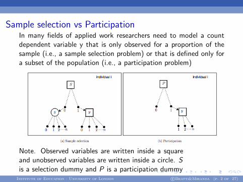
Particiapation + TreatmentOften the count dependent variable is, itself, function of a dichoto-mous variable that indicates a treatment condition T
Motivation Previous work The model Application Results Conclusions References
Particiapation + TreatmentOften the count dependent variable is, itself, function of a dichoto-mous variable that indicates a treatment condition T
Note. Solid arrows indicate functional relationships. x, z,and r are vectors of explanatory variables. ζ and ξ arerandom errors. β, γ, θ are vectors of coefficients. And δand ϕ are coefficients
Institute of Education · University of London c©Bratti & Miranda (p. 3 of 28)
Note. Solid arrows indicate functional relationships. x, z, and r arevectors of explanatory variables. ξ and ψ are random errors. β, γ,abd θ are vector of coefficients. And δ and ϕ are coefficients
Institute of Education · University of London c©Bratti&Miranda (p. 3 of 27)
Example
I Effect of physician advice on individual alcohol consumption(Kenkel et al. 2001)
Institute of Education · University of London c©Bratti&Miranda (p. 4 of 27)

The challenge
The participation (sample selection) and treatment dummies areboth likely to be endogenous. In the drinking example:
I Health ‘oriented’ individuals are more likely to to seek adviceand less likely to participate (drink), and abuse drinking givenparticipation
I Individuals who have been given advice against drinking areless likely to participate
I Physicians are less likely to give advise to individuals with lowlevels of consumption
Institute of Education · University of London c©Bratti&Miranda (p. 5 of 27)
The aim
We aim to develop methods to deal with an endogenous participa-tion (or a sample selection) problem together with an endogenoustreatment problem in a model for a count variable
The method should be able to deal with cases in which unobservedfactors affecting sample selection or participation are correlated withthose affecting exposure to the treatment and those relevant for theintensive margin of the activity of interest (smoking, drinking, etc.)
Institute of Education · University of London c©Bratti&Miranda (p. 6 of 27)
Previous workTo the best of our knowledge, there are models that are able toaddress only one of these issues at the time, or that address a similar– but not exactly the same – issue
I Endogenous participation (selection) and endogenoustreatment
I Terza et al. (2008) propose a two-step estimator for adependent variable observed in interval form to model sampleselection and endogenous treatment;
I Li and Trivedi (2009) use a Bayesian approach to estimate amodel for a continuous and non negative dependent variablewith endogenous participation and multivariate treatments
I Endogenous participation or endogenous treatmentI Greene 2009 (excellent review)
I Kenkel and Terza (2001), which will be described later in moredetails
Institute of Education · University of London c©Bratti&Miranda (p. 7 of 27)
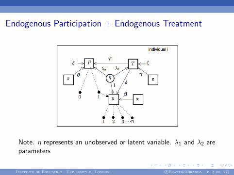
Endogenous Participation + Endogenous Treatment
Motivation Previous work The model Application Results Conclusions References
EPET-Poisson model
Endogenous Participation + Endogenous Treatment
Note. η represents an unobserved or latent variable. λ1 andλ2 are parameters.
Institute of Education · University of London c©Bratti & Miranda (p. 8 of 28)
Note. η represents an unobserved or latent variable. λ1 and λ2 areparameters
Institute of Education · University of London c©Bratti&Miranda (p. 8 of 27)
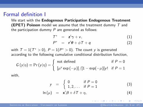
Formal definition IWe start with the Endogenous Participation Endogenous Treatment(EPET) Poisson model we assume that the treatment dummy T andthe participation dummy P are generated as follows:
T ∗ = z′γ + v , (1)
P∗ = r′θ + φT + q (2)
with T = 1(T ∗ > 0), P = 1(P∗ > 0). The count y is generatedaccording to the following cumulative conditional distribution function,
G (y |η) ≡ Pr (y |η) =
{not defined if P = 0
[µy exp (−µ)] /[1− exp(−µ)]y ! if P = 1
with,
y =
{0 if P = 01, 2, . . . if P = 1
(3)
ln (µ) = x′β + δT + η, (4)
Institute of Education · University of London c©Bratti&Miranda (p. 9 of 27)

Formal definition IIAn important feature of the EPET Poisson model is the y = 0 countis generated by a different data generating mechanism from y > 0counts. This is equivalent to say that the decisions
I To drink vs. not to drink
I # of drinks, given current drinking status
are different and should be modelled separately, although the twoprocesses may be correlated
Correlation between T , P and y is induced by imposing some struc-ture on the residuals of equations (1) and (2),
v = λ1η + ζq = λ2η + ξ,
(5)
Institute of Education · University of London c©Bratti&Miranda (p. 10 of 27)
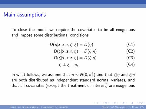
Main assumptions
To close the model we require the covariates to be all exogenousand impose some distributional conditions
D(η|x, z, r, ζ, ξ) = D(η) (C1)
D(ζ|x, z, r, η) = D(ζ|η) (C2)
D(ξ|x, z, r, η) = D(ξ|η) (C3)
ζ ⊥ ξ | η, (C4)
In what follows, we assume that η ∼ N(0, σ2η) and that ζ|η and ξ|η
are both distributed as independent standard normal variates, andthat all covariates (except the treatment of interest) are exogenous
Institute of Education · University of London c©Bratti&Miranda (p. 11 of 27)
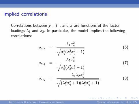
Implied correlations
Correlations between y , T , and S are functions of the factorloadings λ1 and λ2. In particular, the model implies the followingcorrelations:
ρη,v =λ1σ
2η√
σ2η(λ2
1σ2η + 1)
(6)
ρη,q =λ2σ
2η√
σ2η(λ2
2σ2η + 1)
(7)
ρv ,q =λ1λ2σ
2η√
(λ21σ
2η + 1)(λ2
2σ2η + 1)
. (8)
Institute of Education · University of London c©Bratti&Miranda (p. 12 of 27)
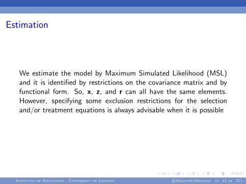
Estimation
We estimate the model by Maximum Simulated Likelihood (MSL)and it is identified by restrictions on the covariance matrix and byfunctional form. So, x, z, and r can all have the same elements.However, specifying some exclusion restrictions for the selectionand/or treatment equations is always advisable when it is possible
Institute of Education · University of London c©Bratti&Miranda (p. 13 of 27)
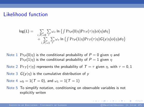
Likelihood function
log(L) =∑
i,Pi =0
∑τωτ ln
{∫PrP(0|η)PrT (τ |η)φ(η)dη
}
+∑
i,Pi =1
∑τωτ ln
{∫PrP(1|η)PrT (τ |η)G (y |η)φ(η)dη
}
Note 1 PrP(0|η) is the conditional probability of P = 0 given η andPrP(1|η) is the conditional probability of P = 1 given η
Note 2 PrT (τ |η) represents the probability of T = τ given η, with τ = 0, 1
Note 3 G (y |η) is the cumulative distribution of y
Note 4 ω0 = 1(T = 0), and ω1 = 1(T = 1)
Note 5 To simplify notation, conditioning on observable variables is notexplicitly writen
Institute of Education · University of London c©Bratti&Miranda (p. 14 of 27)
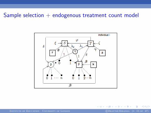
Sample selection + endogenous treatment count model
Motivation Previous work The model Application Results Conclusions References
SET-Poisson model
Sample selection + endogenous treatment count model
Institute of Education · University of London c©Bratti & Miranda (p. 16 of 28)
Institute of Education · University of London c©Bratti&Miranda (p. 15 of 27)

SET-PoissonIn the Sample Selection Endogenous Treatment (SET) Poissonmodel we assume that the treatment dummy T and the sampleselection dummy S are generated as follows:
T ∗ = z′γ + λ1η + ζ, (9)
S∗ = r′θ + ϕT + η + ξ (10)
with T = 1(T ∗ > 0), S = 1(S∗ > 0) and,
F (y |η) ≡ Pr (y |η) =
{not defined if S = 0
[µy exp (−µ)] /y ! if S = 1.(11)
y =
{missing if S = 00, 1, 2, . . . if S = 1,
(12)
ln (µ) = x′β + δT + η, (13)
Institute of Education · University of London c©Bratti&Miranda (p. 16 of 27)
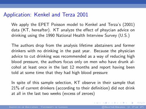
Application: Kenkel and Terza 2001
We apply the EPET Poisson model to Kenkel and Terza’s (2001)data (KT, hereafter). KT analyze the effect of phsycian advice ondrinking using the 1990 National Health Interview Survey (U.S.)
The authors drop from the analysis lifetime abstainers and formerdrinkers with no drinking in the past year. Because the physicianadvice to cut drinking was recommended as a way of reducing highblood pressure, the authors focus only on men who have drunk al-cohol at least once in the last 12 months and report having beentold at some time that they had high blood pressure
In spite of this sample selection, KT observe in their sample that21% of current drinkers (according to their definition) did not drinkat all in the last two weeks (excess of zeroes)
Institute of Education · University of London c©Bratti&Miranda (p. 17 of 27)
Application: Kenkel and Terza 2001Excess zeros:
I recent quitters or people who were actively trying to stopdrinking all together in the last 12 months
I individuals who drink only in very special occasions such asweddings, birthdays, or Christmas day (occasional drikers)
I ‘frequent’ drinkers who, by chance, did not drink any alcoholin the past two weeks; although this last scenario is less likely
Since KT compute drinking as ‘the product of self-reported drinkingfre- quency (the number of days in the past two weeks with anydrinking) and drinking intensity (the average number of drinks ona day with any drink- ing)’, (p. 171-172), the measure refers tothe last two weeks, a su?ciently long time-span. For this reason, weexpect the first two explanations above to be more relevant in thisspecific case
Institute of Education · University of London c©Bratti&Miranda (p. 18 of 27)

Application: Kenkel and Terza 2001
KT account for this excess zero by using a flexible functional formfor the conditional mean of drinking based on the inverse Box-Coxtransforma- tion. In contrast, here we account for it using a stan-dard Poisson model, but treating the zeros and the positive drinkingoutcomes as if they were generated by two separate DGPs.
Our idea is that the DGP for occasional drinkers or quitters shouldbe a different one from that ruling day-by-day drinking by frequentdrinkers
Institute of Education · University of London c©Bratti&Miranda (p. 19 of 27)
Results
We estimated several models:
I A Poisson model
I An Endogenous Treatment (ET) Poisson model (neglectingendogenous participation)
I An EPET model
In what follows all estimations by MSL use 1600 Halton draws toperform the integration. Re-estimating the models with 2000draws did not change significantly coe?cient or standard errors
Institute of Education · University of London c©Bratti&Miranda (p. 20 of 27)

Sample selection + endogenous treatment count model
30
Table 2 Marginal effects of physician advice on the number of drinks consumed in the last two weeksand on the probability of drinking
ET- EP- EPET-Poisson Probit Poisson Poisson Poisson
y(a) Pr(y>0)(b) y(a) Pr(y>0)(b) y>0(a) Pr(y>0)(b) y>0(a)
(1) (2) (3) (4) (5) (6) (7)
Physician advice (T ) 3.679*** 0.079*** -5.395*** 0.079*** 3.377*** -0.045 -4.072***(.558) (.017) (.386) (.017) (.557) (.049) (.864)
ρη,v 0.832*** 0.689***(.029) (.092)
ρη,q .082 0.378***(.141) (.088)
ρv,q 0.261***(.084)
σ2η 2.190*** 1.207*** 1.456***
(.069) (.023) (.099)
N.obs. 2,467 2,467 2,467 2,467 2,467Log-likelihood -32,263 -1,247 -10,184 -8,660 -10,062
Pr(y = 0)(c)
0.00 0.21 0.11 0.21 0.22BIC(d) 70,360 23,418 20,675 20,671
*** significant at 1%. Eicker-Huber-White robust standard errors in parentheses.(a) The marginal effect is computed for a discrete change in T (from 0 to 1) at the sample median of the dependent variable, in analogy to KT;
(b) The marginal effect is computed for a discrete change in T (from 0 to 1) at the sample mean of the other independent variables;
(c) Probability of the zero outcome predicted by the model.
(d) Bayesian information criterion. For the sake of comparability all BICs refer to a three-equation model. In the ET-Poisson the BIC refers to the ET-Poissonand the probit equation for exogenous participation; in the EP-Poisson the BIC refers to the EP-Poisson and the probit equation for exogenous treatment. TheBIC in columns (1)-(2) refers to the probit models for exogenous participation and exogenous treatment and the Poisson model with exogenous participation andexogenous treatment (including the zeros).
Note. y is the number of alcoholic drinks consumed in the last two weeks, Pr(y>0) the probability of drinking in the last two weeks, y>0 the number of alcoholic
drinks consumed in the last two weeks conditional on drinking and T a dichotomous indicator of individual treatment status. Estimation refers to the 1990
NHIS with the sample selection and covariates used in KT. ET, EP and EPET stand for Endogenous Treatment, Endogenous Participation and Endogenous
Participation Endogenous Treatment, respectively. ET-Poisson, EP-Poisson and EPET-Poisson models were estimated using MSL and 1, 600 Halton draws. The
joint Wald test statistic for ρy,T = ρy,P = ρT,P = 0 in the EPET-Poisson model, distributed as a χ2(3), is 57.904 (p-value=0.00).
Institute of Education · University of London c©Bratti&Miranda (p. 21 of 27)
Notes
I *** significant at 1%. Eicker-Huber-White robust standard errors in parentheses.
I (a) The marginal effect is computed for a discrete change in T (from 0 to 1) at the sample median of thedependent variable, in analogy to KT;
I (b) The marginal effect is computed for a discrete change in T (from 0 to 1) at the sample mean of theother independent variables;
I (c) Probability of the zero outcome predicted by the model.
I (d) Bayesian information criterion. For the sake of comparability all BICs refer to a three-equation model.In the ET-Poisson the BIC refers to the ET-Poisson and the probit equation for exogenous participation; inthe EP-Poisson the BIC refers to the EP-Poisson and the probit equation for exogenous treatment. TheBIC in columns (1)-(2) refers to the probit models for exogenous participation and exogenous treatmentand the Poisson model with exogenous participation and exogenous treatment (including the zeros).
I Note. y is the number of alcoholic drinks consumed in the last two weeks, Pr(y>0) the probability ofdrinking in the last two weeks, y>0 the number of alcoholic drinks consumed in the last two weeksconditional on drinking and T a dichotomous indicator of individual treatment status. Estimation refers tothe 1990 NHIS with the sample selection and covariates used in KT. ET, EP and EPET stand forEndogenous Treatment, Endogenous Participation and Endogenous Participation Endogenous Treatment,respectively. ET-Poisson, EP-Poisson and EPET-Poisson models were estimated using MSL and 1, 600Halton draws. The joint Wald test statistic for ρy,T = ρy,P = ρT,P = 0 in the EPET-Poisson model,
distributed as a χ2(3), is 57.904 (p-value=0.00).
Institute of Education · University of London c©Bratti&Miranda (p. 22 of 27)
Main findings
I Neglecting the potential endogeneity of the treatmentproduces wrongly signed estimates of the treatment effects
I Neglecting endogenous participation leads to an overestimateof the treatment effects
I The EPET Poisson model produces estimates of thetreatment effects that are in between those produced by theET Poisson model and the estimates by KT
Institute of Education · University of London c©Bratti&Miranda (p. 23 of 27)
Remark
The EPET Poisson model also allows the same covariates to havedifferent effects on the the intensive and the extensive drinking mar-gins
Institute of Education · University of London c©Bratti&Miranda (p. 24 of 27)

Conclusions
In this paper, we:
I Propose a model suitable for all cases in which an endogenoustreatment affects a count outcome variables, and in whichthere are endogenous participation or sample selection issues
I Show that accounting for the endogeneity of the treatmentstatus and endgenous participation issues is paramount toobtaining consistent estimates of treatment effects, using datafrom KT study of physician advice on drinking
In the future the are plans to make the model’s code available tothe general public through a Stata’s ado file
Institute of Education · University of London c©Bratti&Miranda (p. 25 of 27)
Thanks!
Institute of Education · University of London c©Bratti&Miranda (p. 26 of 27)
ReferencesI Bratti M. and Miranda A (2011). Endogenous treatment effects for count data
models with endogenous participation or sample selection. Health Economics 20(9): 1090–1109.
I Greene, W., 2009. Models for count data with endogenous participation.Empirical Economics 36, 133–173.
I Kenkel, D., Terza, J., 2001. The e?ect of physician advice on alcohol con-sumption: Count regression with an endogenous treatment e?ect. Journal ofApplied Econometrics 16, 165–184.
I Li, Q., Trivedi, P. K., 2009. Impact of prescription drug coverage on drugexpenditure of the elderly – evidence from a two-part model with endogeneity,mimeo.
I Riphahn, R., Wambach, A., Million, A., 2003. Incentive e?ects in the demandfor health care: A bivariate panel count data estimation. Journal of AppliedEconometrics 4, 387–405.
I Terza, J. V., Kenkel, D. S., Lin, T.-F., Sakata, S., 2008. Care-giver advice as apreventive measure for drinking during pregnancy: Zeros, categorical outcomeresponses, and endogeneity. Health Economics 17, 41–54.
I Windmaijer, F., Santos Silva, J., 1997. Endogeneity in count data models: Anapplication to demand for health care. Journal of Applied Econometrics 12,281–94.
Institute of Education · University of London c©Bratti&Miranda (p. 27 of 27)


![Effects of Endogenous Dopamine on Measures of [lsF]N ...€¦ · SYNAPSE 9~195-207 (1991) Effects of Endogenous Dopamine on Measures of [lsF]N-Methylspiroperidol Binding in the Basal](https://img.pdfslide.us/doc/110x75/5f0d4a847e708231d4399e2e/effects-of-endogenous-dopamine-on-measures-of-lsfn-synapse-9195-207-1991.jpg)