Embed Size (px)
Citation preview

Eliciting temptation and self-control through menu choices: a lab
experiment
⇤
Séverine Toussaert
†
February 11, 2016
Abstract
Unlike present-biased individuals, Gul and Pesendorfer (2001) agents may pay to restrict
choice sets despite expecting to resist temptation, thus eliminating self-control costs. I design
an experiment to identify these self-control types, where the temptation was to read a story dur-
ing a tedious task. The identification strategy relies on a two-step procedure. First, I measure
commitment demand by eliciting subjects’ preferences over menus, which did or did not allow
access to the story. I then implement their preferences using a random mechanism, allowing me
to observe subjects who faced the choice, yet preferred commitment. A quarter to a third of
subjects can be classified as self-control types according to their preferences. Of those facing
the choice, virtually all self-control types behaved as they anticipated and resisted temptation.
These findings suggest that policies restricting the availability of tempting options could have
much larger welfare benefits than predicted by present bias models.
JEL classification: C91, D03, D83, D99
Keywords: temptation; self-control; menu choice; curiosity; experiment
⇤I would like to thank my advisors David Cesarini and Guillaume Fréchette for their support and continuousfeedback in the development of this project. I also thank Anwar Ruff for teaching me how to program experimentsand Margaret Samahita for her assistance during the experimental sessions. Finally, I wish to thank Ned Augenblick,Marina Agranov, Andrew Caplin, Micael Castanheira, Mark Dean, Kfir Eliaz, Xavier Gabaix, Yves Le Yaouanq,Barton Lipman, Daniel Martin, Efe Ok, Pietro Ortoleva, Jacopo Perego, Giorgia Romagnoli, Ariel Rubinstein,Emanuel Vespa, Sevgi Yuksel and seminar participants at NYU and University of Michigan for their useful comments.
†New York University, Department of Economics. Contact: [email protected] or +1 646 610 9813. Website:http://cess.nyu.edu/sev/
1

1. Introduction
Models of dynamically inconsistent time preferences (Strotz [1956], Laibson [1997], O’Donoghue and
Rabin [1999]) are by far the most popular framework in the literature on self-control problems. A
central implication of these models is that present-biased agents may demand commitment devices
to constrain the choices of their future selves. As an alternative approach, Gul and Pesendorfer
(2001) (henceforth GP 2001) generate commitment demand by modeling agents whose preferences
not only depend on final consumption but also on the most tempting alternative in the choice set.
One key distinction between these theories pertains to the motives that drive a decision maker to
restrict his choice set. While a present-biased agent will choose to eliminate a temptation from his
choice set only if he expects to succumb to it, a GP agent may value commitment even if he expects
to resist temptation, because commitment eliminates the cost of exerting self-control. The present
paper takes a first step to quantify the importance of these “self-control types” who may prefer to
remove a temptation from their choice set, despite expecting not to succumb to it.
Assessing the prevalence of self-control types is important from a policy perspective: if unchosen
alternatives can affect welfare, then policies designed to reduce the availability of tempting options
could have strong welfare effects. To see this, consider the welfare implications of introducing
smoking bans in public spaces. Both of the above theories predict that current smokers who are
trying to quit could benefit from a ban; what GP 2001 further suggests is that a ban could also
increase the welfare of former smokers by alleviating the self-control costs of remaining smoke-free.
Welfare calculations that fail to account for these costs could therefore substantially underestimate
the welfare benefits of smoking bans. Ignoring self-control costs may not only bias our estimate
of the effect size of a given policy but also our assessment of the type of policy tools likely to be
most effective. If self-control is high so that tempted agents rarely succumb to temptation, then
price policies such as proportional taxes or subsidies will be ineffective, for their aim is to alter
consumption behavior.1 On the other hand, policies that impose a cap on consumption of the
tempting good may improve welfare even for those whose consumption would be below the cap in
the absence of restrictions.
While the above discussion illustrates the importance of measuring self-control costs, it also1See Krusell and Smith (2007, WP) who show in a dynamic general equilibrium model that proportional subsidies
on investment are a useful policy tool only if self-control is low and agents usually succumb to the temptation tooverconsume, as is the case of present-biased agents.
2

hightlights the empirical challenge pertaining to the identification of the population incurring these
costs: to identify self-control types, one not only needs to observe whether they would prefer to
restrict their choices, but also what they would do in a counterfactual world where no form of
commitment is available. However, with naturally occurring data, we rarely observe individuals
having a preference for a restricted choice set A and yet receiving a larger choice set B. To tackle
this empirical challenge, I design an experimental method that tests for the prevalence of self-control
types and implement it in a laboratory setting.
In the experiment, the potential temptation was to forego additional earnings to learn a sensa-
tional story while performing a tedious attention task for which subjects received payment. I adopt
a two-step procedure to identify subjects who suffer from self-control costs. First, using an incentive
compatible mechanism, I elicit subjects’ preference ordering over a set of menus, which either did
or did not allow access to the story during the task and classify subjects into types according to
their menu preferences. A self-control type is a subject who would strictly prefer to (i) remove the
temptation from his choice set instead of facing the choice; (ii) face the choice instead of receiving
the tempting option for sure, as he expects to resist it. Second, I implement subjects’ preferences
using a random implementation rule. This mechanism allows me to observe the behavior of subjects
who faced the choice, yet preferred commitment and to contrast perceived self-control with actual
self-control. Finally, I gather two types of auxiliary data to provide additional evidence in favor of
the GP model. First, I measure subjects’ beliefs about their anticipated choice in the absence of
commitment to study whether those classified as self-control types indeed expect to resist tempta-
tion. Second, I contrast the task performance of subjects who faced the choice with those who faced
commitment to study whether the mere exposure to learning opportunities entailed a self-control
cost in the form of a productivity loss.
Depending on how conservative one wants to be, I find that between 23% and 36% of subjects
can be classified as self-control types according to their menu preferences, a proportion which is 3
to 4 times higher than what would be observed if subjects had ordered the menus at random. This
is by far the most common preference pattern among those who preferred to restrict their access
to the story; in contrast, only 2.5% of subjects exhibit menu preferences consistent with standard
models of dynamic inconsistency. In line with the GP model, almost all self-control types predicted
that they would resist the temptation to learn the story in the absence of commitment. Finally,
perceived self-control, as measured by subjects’ menu preferences and anticipated choices, almost
entirely coincides with actual self-control when facing the choice: while 18% of subjects chose to
3

learn the story when offered the choice, all but one subject with self-control preferences succumbed
to the temptation to do so. At the same time, task performance in the full sample was lower in the
absence of commitment, which provides suggestive evidence that resisting learning opportunities
might have entailed a self-control cost.
To my knowledge, this is the first study specifically designed with the intention of identifying
self-control types and measuring their prevalence in a controlled setting. As such, the present
paper relates to a vast literature that explores the connections between self-control problems and
commitment demand, both in laboratory experiments (Houser et al. [2010], Augenblick et al. [2015])
and in field settings (Ashraf at al. [2006], Kaur et al. [2010], John [2015], Sadoff et al. [2014]).
This paper is also connected to a burgeoning literature studying commitment and flexibility through
menu choice. Dean and McNeill (2015) explore the relationship between preference uncertainty and
preference for larger choice sets by linking preferences over menus of work contracts to subsequent
choices of contracts; they find no evidence of preference for commitment in their setting. In the
context of a weight loss challenge, Toussaert (2014) studies participants’ preferences over lunch
reimbursement options differing in their food coverage and finds a strong demand for eliminating
unhealthy foods from the coverage; however, the actual food selections were not observed.
The remainder of this paper is organized as follows. Section 2 introduces the theoretical frame-
work on which the experiment is based. Section 3 outlines the experimental design and Section
4 presents the experimental results. Section 5 concludes. Additional results are reported in the
Appendix at the end of this paper as well as in an Online Appendix (OA).
2. Temptation and self-control through menu choices
The analysis of this paper is grounded in the theory of menu choice of Gul and Pesendorfer (2001),
which provides a framework for studying costly self-control. This section describes how temptation
and self-control are elicited in GP 2001, explains key distinctions and connections with other models
of temptation and discusses the restrictions imposed by the theory on choice behavior.
2.1 Costly self-control in GP 2001
GP 2001 consider a two-period expected utility model, t 2 {1, 2}. Their primitive is a preference
relation ⌫1 defined on a set M of menus (of lotteries). In Period 1, a decision maker (DM) chooses
among menus according to ⌫1, with the interpretation that in Period 2, he will make a choice from
4

the selected menu according to ⌫2. In addition to the usual assumptions,2 GP 2001 impose a new
behavioral axiom on ⌫1 called Set Betweenness, which states that for any two menus A and B,
A ⌫1 B implies A ⌫1 A [B ⌫1 B
This axiom allows to capture behaviorally the notions of temptation and self-control. To see how,
consider a simple choice situation with two options a (for apple) and b (for brownie) and assume
that the ex ante preferences of the DM are such that {a} �1 {b}. A standard DM (STD) evaluates
a menu by its best element(s) and is unaffected by the presence of dominated options, implying that
{a} ⇠1 {a, b} �1 {b}. On the other hand, a DM who is tempted by the brownie would prefer to
commit to a menu that excludes b than to be facing the choice between a and b in Period 2. In other
words, b is a temptation for a if {a} �1 {a, b}. In this model, there are two reasons why a tempted
DM may favor commitment to a. First, the DM may expect to give in to b if offered to choose
from {a, b}, thus assigning the same value to {b} and {a, b}. Alternatively, the DM may anticipate
that he will resist b when facing {a, b} by exerting self-control, which makes {a, b} more valuable
than {b}. In formal terms, say that (i) b is an overwhelming temptation if {a} �1 {a, b} ⇠1 {b} and
(ii) b is a resistible temptation if {a} �1 {a, b} �1 {b}. In the experiment, a DM with the menu
preferences {a} �1 {a, b} �1 {b} will be called self-control type. GP 2001 show that under their
axioms, ⌫1 admits the following self-control representation
V
GP
(A) := maxx2A [u(x) + v(x)]� max
y2Av(y)
The commitment utility u measures utility in the absence of temptation i.e. when committed to
a singleton choice. The temptation utility v measures the temptation value of an alternative and
maxy2Av(y)� v(x) is the self-control cost of choosing x over the most tempting alternative in A.3
In Period 2, the DM chooses as if he maximized the compromise utility u+ v.
2⌫1 is required to be a weak order, which satisfies the standard expected utility axioms of Continuity and In-dependence adapted to a menu choice setting. These technical axioms are not tested in this paper and are treatedas maintained assumptions. The requirement that ⌫1 be a weak order is also assumed away in the experiment, forsubjects are required to provide a full ranking (allowing for ties) of the alternatives, thus automatically satisfyingcompleteness and transitivity. See Section 3.2 for more details.
3To see why u is a commitment utility, let A = {a} and notice that V
GP
(A) = u(a). To see why v measurestemptation, notice that if u(a) > u(b) and v(b) > v(a) then V
GP
({a}) > V
GP
({a, b}) i.e. the agent is tempted by b.
5

2.2 Connections and differences with other theories
The GP model presents several distinguishing features, which guide the identification of self-control
types. First, commitment in the GP model can be rationalized through two channels: either by
the DM’s belief that he will give in to temptation or because commitment eliminates the cost of
exerting self-control. In contrast, standard models of dynamic inconsistency can only rationalize
the case of overwhelming temptation, {a} �1 {a, b} ⇠1 {b}.4 The reason is that the preferences
of a present-biased agent only depend on final consumption and not on the specific set from which
consumption is taken; as a result, commitment can only be valuable if the agent expects to deviate
from the ex ante optimal consumption path. As such, models of present bias can be understood as
a limit case of the GP model when the self-control cost becomes arbitrarily large, so that the agent
never exercises self-control.5
Secondly, although observing the preference ordering {a} �1 {a, b} �1 {b} is generally enough to
distinguish the GP model from standard models of dynamic inconsistency, this is only true under the
most common assumption that Period 2 choice is deterministic. To see this, suppose that the DM
is uncertain about his future temptation: with probability p, he expects to succumb to temptation
and select b, while with probability (1� p), he believes that he will face no temptation and choose
a. For such a DM, the preference ordering {a} �1 {a, b} �1 {b} does not reflect costly self-control;
rather, it is explained by a probability p 2 (0, 1) of indulgent behavior.6 Therefore, to be able to
distinguish between these two interpretations (costly self-control versus random indulgence), it is
necessary to enrich the dataset to include expectations about Period 2 choice from {a, b}: only a
DM who suffers from random indulgence will expect to give in with positive probability.
Third, Gul and Pesendorfer model a sophisticated agent who correctly anticipates the choice he
will make in Period 2 from the selected menu and chooses a menu in Period 1 accordingly. Formally,
say that a DM is sophisticated if A[{x} �1 A implies x �2 y for all y 2 A. In other words, if a DM4By standard, I mean models that assume a fixed present bias parameter and degenerate beliefs about the size of
this bias, the most common assumptions in this literature.5GP 2001 show that the limit case in which the agent never exercises self-control can be obtained in their
framework by relaxing continuity; in this case, the DM’s preferences have a Strotz representation V
S
(A) :=max
x2A
u(x) subject to v(x) � v(y) for all y 2 A. In words, the DM chooses in Period 2 as if he lexicographicallymaximized the temptation utility and then the commitment utility. Under specific functional-form assumptions,Krusell et al. (2010) show that the GP model nests the multiple-selves model of Laibson (1997), which correspondsto the specific case in which their temptation strength parameter � - governing the cost of self-control - tends toinfinity.
6This point has been formally addressed by Dekel and Lipman (2012), who show that any menu preference ⌫1
which admits a (possibly random) GP representation also has a random Strotz representation (see previous footnote),where the utility v is uncertain.
6

values the addition of an alternative x to menu A, it must be because he correctly anticipates that
he will choose x over any element of A in Period 2. It can be shown that sophistication is a necessary
condition for ⌫2 to comply with the above interpretation of ⌫1, that is, for ⌫2 to be represented
by the utility u + v (Kopylov [2012], Thm 2.2). As a consequence, the GP model cannot capture
the behavior of a (partially) naive agent for whom {a} ⌫1 {a, b} �1 {b} and yet b �2 a. In the
experiment, it will be useful to distinguish perceived self-control (identified by {a} �1 {a, b} �1 {b})
from actual self-control (identified by {a} �1 {a, b} �1 {b} and a �2 b). This will be done by first
eliciting subjects’ menu preferences and then contrasting these preferences with the actual choices
made from the flexible menu.
Finally, Set Betweenness imposes several restrictions on choice behavior, which preclude two
interesting phenomena. First, a DM who behaves according to the GP model cannot exhibit a strict
preference for flexibility (that is, {a, b} �1 {a}, {b}). As a result, the GP model cannot accommodate
the fact that an agent who feels uncertain about his future tastes may want to keep his options open,
an idea originally motivated by Kreps (1979). Secondly, Set Betweenness gives a special structure
to the form of temptation by excluding the possibility that {a} �1 {b} �1 {a, b}. Such a preference
profile could be motivated by the agent’s anticipated feeling of guilt if he chooses the tempting
option b from {a, b}, while he could have acted virtuously by selecting a. Such an interpretation
has been formalized by Kopylov (2012) who proposes a relaxation of the Set Betweenness axiom
allowing to capture guilt. These preferences (FLEX, GUILT ) will be incorporated in the taxonomy
of types presented in the results section, the prevalence of which will be assessed against the one of
self-control types.
3. Experimental design
The experiment was divided in two periods, followed by an exit survey. Period 1 comprised 5
sections (A-E) described below, pertaining to the elicitation of a potential temptation (Sections A
and B), of menu preferences (Sections C and D) and of beliefs about choices in Period 2 (Section
E). Details about the exit survey are provided at the end of this section, as well as a summary of
the structure of the experiment (Fig.1); see OA-E for the instructions.
7

3.1 Description of the tempting good
The first part of the experiment was devoted to the elicitation of a potential temptation. Generating
temptation in the lab poses several challenges. First, it appears difficult to find a good that is
tempting to a majority of subjects, that is, a good that subjects think they should not consume
and yet find enticing.7 Secondly, the tempting goods commonly considered in the literature such
as surfing the Internet (Houser et al. [2010], Bonein and Denant-Boemont [2015]) or watching an
entertaining TV show (Bucciol et al. [2013]) can be easily obtained outside the lab, which reduces
their immediate appeal. In this experiment, I exploit subjects’ curiosity and, in particular, the
human tendency to like gossiping and hearing gossip about others, which is virtually present in all
human societies (Dunbar [2004]).
The potential temptation was to forfeit money to learn a personal story from one subject in the
room, while performing a tedious task. In Section A, subjects were asked to describe an incredible
or strange life event that they personally experienced. As an aid, they were given three hypothetical
examples. Subjects were given 10 minutes to write their story by hand on a blank form and place
it back in an unnumbered envelope. The stories were then collected by an assistant would selected
the story she considered to be the most incredible and recorded it in the system (see OA-F for the
selected stories).8 Finally, subjects were informed that a new envelope containing a secret code
would be distributed in Period 2 and this code could potentially allow them to read the story on
their screen.
In Section B, subjects were introduced to the main task of Period 2. For a period of up to 60
minutes, subjects were instructed to focus on a four-digit number that was updated on their screen
every second.9 At random times, they received a prompt to enter the last number they saw and the
number was reinitialized after every prompt. All subjects were sent a total of 5 prompts and could
receive $2 per correct answer. After describing the task, subjects were told that two options could
be potentially available in Period 2 depending on their choices in later sections:7For instance, note that for chocolate to be a tempting good, it is not enough that most subjects find chocolate
appealing, they should also perceive that consuming chocolate should be avoided.8Notice that subjects’ curiosity for the selected story could have been due to 1) their eagerness to read about
the personal story of someone else in the room and/or 2) their desire to know whether the story was theirs. 70% ofsubjects declared to be at least somewhat interested in learning the story for one of these two motives, with the firstmotive being the primary source of curiosity (see OA-B).
9During the first session, Period 2 was announced to last exactly 60 minutes; however, given the boredom expe-rienced by most subjects and the overall length of the session, the duration of the task was reduced to 45 minutes.The other 5 sessions had the same task duration of 45 minutes with random prompts occurring at the same time; theonly difference was that subjects were told that the task could last “up to” 60 minutes. Since no major differences inbehavior were observed relative to Session 1, all sessions will be pooled in the data analysis.
8

“No Learning” (0): do the task without learning the story and receive payment for all 5 prompts.
“Learning” (1): learn the story during the task and receive payment for 4 of the 5 prompts selected
at random.
Regardless of the option, subjects worked on the task for the same duration and received feedback
about their performance and earnings only at the end of the experiment. To minimize communica-
tion opportunities after the experiment, subjects were told that they would be requested to leave
the lab one at a time; furthermore, no student could a priori know who learned the story in their
session. As a result, it was difficult for a subject to satisfy his curiosity for this specific piece of
information outside of the context of the experiment. Finally, subjects practiced with the task for
2 minutes and received feedback about their performance during that practice period.
3.2 Elicitation of menu preferences
To identify temptation and perceived self-control, Sections C & D elicited subjects’ preferences over
a list of three “menus”, one of which was assigned to them at the start of Period 2:
Menu “Pre-Select No Learning” {0}: eliminates the chance to learn the story in Period 2 and
pays for all 5 prompts; practically, the box where the secret code could be entered to access the
story was removed from the subject’s screen.
Menu “Pre-Select Learning” {1}: commits to learning the story in Period 2 and pays for only
4 of the 5 prompts; the story could be accessed at any time during the task but was automatically
displayed at the end if not displayed before.
Menu “Decide in Period 2” {0, 1}: offers the opportunity to decide during the attention task
whether and when to learn the story by entering the secret code.
The elicitation of subjects’ weak ordering ⌫1 over the set M = {{0}, {1}, {0, 1}} was performed in
two steps (Sections C & D). In Section C, subjects were asked to assign a rank number 1, 2 or 3
to the three menus presented in a list.10 To allow for the expression of indifferences, subjects could
assign the same rank number to two or all three menus. Before providing their ranking, subjects10To minimize order effects, subjects were randomly assigned to one of two list orders: l1 = ({0, 1}, {1}, {0}) or
l2 = ({1}, {0}, {0, 1}), meaning that the flexible menu was presented either at the top or at the bottom, and {0}never appeared at the top. Because options listed first are in general more likely to be assigned rank 1 than thoselisted last, this design feature should have if anything reduced the likelihood of observing temptation (understood asa strict preference for {0}). Ranking differences across the two lists were not found to be significant.
9

were told that they would be assigned a menu at the start of Period 2 based on the following
procedure:
1. With probability 1/2, a subject received {0, 1} regardless of his ranking.
2. With probability 1/2, a subject’s ranking was implemented stochastically such that the odds
of receiving a given menu were increasing in its ranking, as displayed in the following table:
Ranking of (X,Y ,Z) % chance of being drawn (%X
,%Y
,%Z
)(1,2,3) (50,30,20)(1,1,2) (40,40,20)(1,2,2) (50,25,25)(1,1,1) (33.3,33.3,33.3)
The above elicitation procedure has two important properties. First, it makes it incentive compatible
for a subject with a strict rank ordering �1 to report his true preferences. Secondly, because the
menu preferences are only implemented probabilistically, one can observe the behavior of subjects
who faced the flexibility of choice and yet preferred commitment. As a result, one can contrast
perceived self-control, as revealed by subjects’ rank ordering, with actual self-control when facing
the flexible menu.
So far this procedure however does not strictly incentivize subjects to report indifferences since
a DM who is indifferent between two menus would also take any probability distribution over these
menus.11 To disentangle indifferences from strict preferences, one needs to obtain a cardinal measure
of preferences. Such a measure was collected in Section D by asking subjects for their willingness
to pay (WTP ) to replace their second choice with their top choice and their last choice with their
second choice. In case a subject was indifferent between two menus, one of them was selected to
be the replaceable option. Subjects were randomly assigned within a session to express their WTP
either in terms of money or in terms of time via a multiple price list mechanism:12
- For the $ WTP , subjects made 8 decisions between [their second (last) choice] and [their top
(second) choice - $X] where X = {0.01, 0.02, 0.05, 0.10, 0.20, 0.30, 0.40, 0.50}.
- For the time WTP , subjects made 8 decisions between [their second (last) choice] and [their top
(second) choice + N minutes on the attention task ] where N = {1, 2, 3, 4, 5, 6, 8, 10}.11Note that this statement is only true under the assumption that the DM satisfies the Independence Axiom (as is
assumed in the Gul and Pesendorfer model, although in a different form).12In the $ WTP condition, the money was taken from the subjects’ show-up fee of $10. In the time WTP condition,
subjects were asked to spend additional minutes on the attention task for no additional payment.
10

To enforce monotonicity, subjects were not allowed to make multiple switches between the two
options. If a subject’s ranking was implemented and their second (last) choice was drawn, then one
of the 8 decisions was chosen for implementation, thus ensuring incentive compatibility.
The purpose of contrasting willingness to pay for time versus money was to assess the extent to
which the expression of a strict preference (in particular, for commitment) might be sensitive to the
unit of payment. Indeed, so far very few studies have found that individuals are willing to pay even
the smallest amount of money for commitment.13 For instance, Augenblick et al. (2015) find that
while 59% of their subjects favor commitment when it is free, the demand is close to zero at a price
as low as $0.25. Although these findings could raise the concern that a demand for commitment
at a price of zero does not reveal a true preference for commitment, another interpretation is that
individuals think differently about money and time (Ellingsen and Johannesson [2009]) and would
have been more willing to pay in terms of their time. Testing for differences in the willingness to
pay across domains therefore offers a way to assess the robustness of the procedure used in this
paper to identify indifferences.
3.3 Elicitation of beliefs
Finally, Section E gathered data on subjects’ beliefs about their likelihood to learn the story in
Period 2 if offered {0, 1}. The measurement of these beliefs served two objectives. First, although
beliefs about ex post choice are generally not a primitive of models of menu preferences, they play
a central role in the interpretation of those models. A GP agent with the preference ordering
{0} �1 {0, 1} �1 {1} must expect to resist the temptation to read the story if offered {0, 1} (that
is, 0 �2 1), while a DM who suffers from random indulgence should expect to succumb some of
the time. Similarly, a “Krepsian” DM with a preference for flexibility {0, 1} �1 {0}, {1} must be
uncertain about his willingness to learn the story if offered {0, 1}. Therefore, gathering belief data
allows to gain further insights into the interpretation of subjects’ preference orderings.
A second reason to collect belief data is to obtain a measure of the gap between predicted and
actual behavior. So far, very few papers in the self-control literature have attempted to measure
sophistication, understood as the ability to predict one’s own behavior in the future. Yet, the
prediction that agents with self-control problems should demand commitment crucially relies on the
assumption of sophistication. It is therefore important to understand the degree to which subjects
mispredict their future behavior and how this might affect their menu preferences.13Two exceptions are Milkman et al. (2014) and Schilbach (2015).
11

The elicitation of individuals’ predictions about their future behavior however poses a method-
ological challenge. Indeed, any payment scheme designed to incentivize subjects to truthfully report
their beliefs will also incentivize changes in the behavior to be predicted. This point has been ac-
knowledged by Acland and Levy (2015) in one of the rare papers to propose an incentivized proce-
dure to elicit an individual’s beliefs about his future behavior.14 An alternative route for measuring
sophistication is through the use of an unincentivized survey instrument such as the one proposed
in Ameriks et al. (2007) and adopted by Wong (2008) and John (2015).
In this paper, I propose a third, incentivized, method to elicit an individual’s beliefs about his
future choices. The idea of the method is to instrument beliefs about oneself with beliefs about a
similar other. More precisely, each subject was asked to guess the future choice (Learning or No
Learning) of another participant in the room who provided the same ranking as them in Section
C. Provided there was such a participant and he could make a choice from {0, 1} in Period 2, a
subject received $2 for a correct guess and 0 otherwise. A priori, there are two reasons to believe
that incentivized beliefs about the future behavior of a similar other could be a strong predictor
of beliefs about one’s own behavior. First, if subjects interpret menu rankings in a way consistent
with theories of menu choice, then one should observe a higher proportion of Learning guesses for
rankings where {0, 1} �1 {0} and/or {0, 1} ⇠1 {1} relative to rankings where {0, 1} �1 {1} and/or
{0, 1} ⇠1 {0}; therefore, the belief of a subject who conditions his guess on a ranking identical
to his own should be highly correlated with what he expects his future choice to be. Secondly,
there is large evidence in economics and psychology that beliefs about others are subjected to a
false consensus effect, which refers to an individual’s tendency to extrapolate from his own type the
behavior of others (Ross et al. [1977], Ellingsen et al. [2010], Butler et al. [2013], Rubinstein and
Salant [2015]). As a result, subjects are likely to form their guess regarding the other participant
assuming similarity on other - possibly unobservable - dimensions than the preference ordering.
To test the strength of the above instrument, subjects were also asked an unincentivized question
about their likelihood to learn the selected story in Period 2 if given the chance. Answers were
expressed on a five-point scale (very unlikely, quite unlikely, unsure, quite likely, very likely); thus
the structure of this question differed from the binary choice frame adopted for the incentivized14In their paper, the authors seek to measure predictions about future gym attendance by eliciting subjects’
willingness to pay for a coupon that pays contingent on attending the gym. With this mechanism, a sophisticatedindividual with self-control problems may have an incentive to overstate his willingness to pay for the coupon asa commitment device to attend the gym more often than initially expected, thus providing a biased estimate ofexpected gym attendance. See also Augenblick and Rabin (2015) who use accuracy payments to elicit beliefs aboutfuture task completion.
12

question. This should have minimized the chances of observing a mechanical correlation between
answers simply due to subjects’ exposure to identically-framed questions.15
3.4 Exit survey
At the end of the session, subjects replied to a short survey designed to better understand (i) their
ranking of the menus, and (ii) their interest for the story. In addition, the survey gathered some
basic demographic and academic information (gender, major, GPA) and subjects were evaluated on
three psychometric scales designed to measure self-control and trait curiosity. A description of the
exit survey variables as well as summary statistics are presented in OA-B.3 and -E.
Figure 1: Timeline of the Experiment
storyselection
taskdescription
| {z }Period 1(40 min)
menuranking
beliefelicitation
attentiontask
| {z }Period 2(45 min)
exitsurvey
4. Results
In this section, I present results using data from 6 sessions conducted at the Center for Experimental
Social Science (CESS) of New York University with a total of 120 subjects recruited from the student
population. Including a $10 show-up fee, average earnings were $18.70 for a little less than two hours.
The first part of this section studies perceived self-control by analyzing the distribution of menu
preferences elicited in Period 1 through the initial rank ordering procedure and subsequent WTP
decisions, and by relating these preferences to subjects’ beliefs about Period 2 choice. The second
part turns to actual self-control by confronting subjects’ menu preferences and beliefs to their actual
choices in Period 2, and by studying task performance under commitment versus flexibility.15At the end of Section E, subjects were also asked questions about their personal interest for the story; see OA-B.
13

4.1 Perceived self-control: menu preferences
4.1.1 Initial rank orderings
Using data from the rank assignments performed in Section C, I classified subjects into menu types,
the distribution of which is presented in Table 1. In principle, subjects could have ranked the three
menus {0}, {1} and {0, 1} in 13 different ways.16 In actuality, 90% of the subjects can be grouped
in one of 7 menu types. As a benchmark, the observed frequencies of menu types are contrasted
with the frequencies that would be expected if subjects picked a rank ordering at random.
Table 1: Main preference orderings
Preference ordering menu type % subjects (N) random benchmark p-value
{0} �1 {0, 1} �1 {1} SSB�0 35.8% (43) 7.7% < 0.001{1} �1 {0, 1} �1 {0} SSB�1 4.2% (5) 7.7% 0.171
{0, 1} �1 {0} �1 {1} FLEX�0 20.8% (25) 7.7% < 0.001{0, 1} �1 {1} �1 {0} FLEX�1 7.5% (9) 7.7% 1.000{0, 1} �1 {1} ⇠1 {0} FLEX�0_1 5.8% (7) 7.7% 0.605
{0, 1} ⇠1 {0} �1 {1} STD�0 9.2% (11) 7.7% 0.494
{0} �1 {1} �1 {0, 1} GUILT 6.7% (8) 7.7% 0.863
other ordering 10.0% (12) 46.1% < 0.001
Total 100% (120) 100%
Notes: The reported p-values correspond to the result of a two-sided binomial test that the observed frequency isequal to the benchmark frequency of selecting one of the 13 rank orderings at random. Option 0 (resp. 1) refers toNo Learning (resp. Learning).
The first two types ranked {0, 1} strictly in between the other two menus and are labelled SSB�i
,
for Strict Set Betweenness with singleton i 2 {0, 1} ranked first. Consistent with the intuition that
learning the story is the source of temptation in this experiment, 90% of subjects who satisfy Strict
Set Betweenness are of type SSB�0. This self-control type is also the most represented category,
with a proportion more than 4 times larger than what would be observed in a random sample
(35.8% versus 7.7%; p < 0.001). The second category of types denoted FLEX�i
corresponds to the
subjects who expressed a strict preference for {0, 1} with i 2 {0, 1, 0_1} as their second best choice.16In addition to the indifference ordering (1,1,1), there are 6 permutations of the ranks (1,2,3), 3 permutations of
(1,1,2) and 3 permutations of (1,2,2).
14

Relative to the benchmark of random choice, only the proportion of FLEX�0 is significantly higher
than what would be expected by chance (20.8% versus 7.7%; p < 0.001). The last two categories
corresponding to the standard DM with no temptation to learn, STD�0, and the flexibility-averse
type GUILT represent a small fraction of the sample. Interestingly, the rank ordering capturing
temptation with no self-control {0} �1 {0, 1} ⇠1 {1} (included in the “other ordering” category) is
underrepresented in this sample (2.5%; p = 0.026 against benchmark). In this respect, standard
models of present-biased preferences - which can only rationalize the ordering {0} �1 {0, 1} ⇠1 {1}
but not {0} �1 {0, 1} �1 {1} - have a low explanatory power in this environment.
4.1.2 Refinement of menu rankings through WTP decisions
The above classification may overestimate the proportion of subjects with a strict preference ordering
as it is solely based on the initial ranking procedure, which does not strictly incentivize subjects to
truthfully report an indifference. To obtain a lower bound estimate on the proportion of self-control
types, I now examine WTP decisions for replacing the second (last) choice in the ranking with the
top (second) choice.
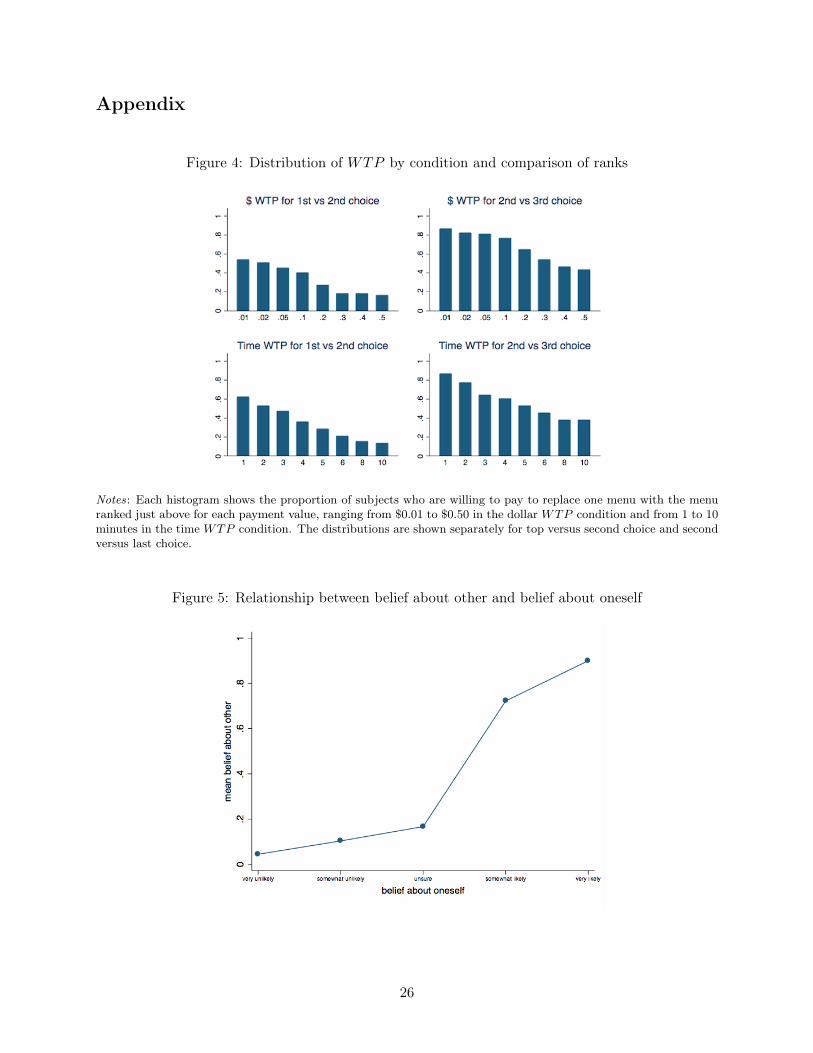
In total, 67 (53) subjects were assigned to the $ (time) WTP condition. No significant differ-
ences were observed across conditions: subjects had a positive WTP in 70% (75%) of the menu
comparisons in the money (time) condition (F -stat = 0.52; p = 0.472); the average switching point
in the list of 8 decisions was 4.01 for money and 3.69 for time (F -stat = 0.56; p = 0.456). Appendix
Fig.4 shows the full distribution of WTP decisions by condition and by comparison of ranks; differ-
ences appear to be quite marginal across conditions. For the rest of the analysis, I therefore convert
the time WTP into a $ WTP in order to evaluate decisions on a single scale. For each of the 7
major preference orderings, Table 2 shows the average WTP to replace one menu with a (weakly)
better ranked menu, as well as the percentage of subjects who had a positive WTP.
Overall, there is a high degree of consistency between subjects’ initial ordering (�1 or ⇠1) and
subsequent WTP (> 0 or = 0), which are coherent with each other in more than 70% of the cases.
First, 62% (87%) of subjects who ranked their top (second) choice strictly above their second (last)
choice also had a strictly positive WTP. For all types except FLEX�0, a majority of subjects
were willing to pay for an option they strictly ranked higher. In particular, 58% of the self-control
types of Table 1 were willing to pay to receive {0} instead of {0, 1}; furthermore, their WTP for
commitment is increasing in their level of curiosity for the story (see OA-B.1). Secondly, as would be
expected from subjects who are indifferent, those who gave the same rank to their top (bottom) two
15

options had a significantly lower WTP than subjects with a strict preference for their top (second
best) option (p = 0.005 for top and p = 0.074 for bottom on a two-sided t-test).17
Table 2: Distribution of WTP by rank ordering
top choice versus second choice second choice versus last choice
average WTP % with WTP > 0 average WTP % with WTP > 0
Preference ordering (all) (freq.) (all) (freq.)
{0} �1 {0, 1} �1 {1} $0.14 58.1% (25/43) $0.31 88.4% (38/43){1} �1 {0, 1} �1 {0} $0.30 80.0% (4/5) $0.38 80.0% (4/5)
{0, 1} �1 {0} �1 {1} $0.07 40.0% (10/25) $0.28 96.0% (24/25){0, 1} �1 {1} �1 {0} $0.23 88.9% (8/9) $0.11 88.9% (8/9){0, 1} �1 {1} ⇠1 {0} $0.10 57.1% (4/7) $0.25 85.7% (6/7)
{0, 1} ⇠1 {0} �1 {1} $0.06 27.3% (3/11) $0.37 81.8% (9/11){0} �1 {1} �1 {0, 1} $0.25 100.0% (8/8) $0.20 62.5% (5/8)
Strict ranking $0.15 62.4% (63/101) $0.28 87.0% (94/108)Indifference $0.05 31.6% (6/19) $0.17 83.3% (10/12)
Notes: Average WTP computed as subjects’ mean WTP pooling dollar and time conditions; the time WTP wasconverted into dollars according to the following formula: ˜
WTP= 0.01 (=0.50) if WTP
t
=1 (=10) and ˜WTP= 0.01
+ 0.5( t�110�1 ) if WTP
t
2 {2, 3, 4, 5, 6, 8}. “Strict ranking” refers to subjects who assigned rank 1 and 2 (resp. 2 and 3)to their top (bottom) two choices, while “Indifference” refers to those who gave rank 1 (2) to their top (bottom) twochoices. Option 0 (resp. 1) refers to No Learning (resp. Learning).
Table 3 presents an alternative classification, which accounts for subjects’ WTP decisions by
replacing �1 with ⇠1 whenever WTP = 0 and ⇠1 with �1 whenever WTP > 0. The fraction
of subjects with temptation and self-control preferences SSB�0 drops to 23.3% (relative to 35.8%
in Table 1), but remains about 3 times higher than what would be observed in a random sample.
The standard DM with no temptation to learn, STD�0, is now the most represented category (30%
of the sample), while the proportion of subjects with a preference for flexibility is divided by two.
In particular, the category FLEX�0_1 almost disappears from the sample and is replaced in the17However, 10 of the 12 subjects who gave the same rank to their bottom two options reported a positive WTP
for one of the options. This high percentage is mostly due to subjects with menu type {0, 1} �1 {0} ⇠1 {1} whomight have expressed their indecisiveness (rather than an indifference) by assigning the same rank to {0} and {1}.Some comments from these subjects give substance to this interpretation:- “I was undecided so I ranked to make my decision later.” (Session 3, id 31)- “I had put Decide in period 2 first so that I could have some choice and effect on which menu I would receive. Iranked the other two options both as 2 because I was unsure at the time of which menu I wanted.” (Session 3, id 40)
16

table by subjects classified as indifferent (IND). However, besides STD�0 and SSB�0, no other
menu type is present in a proportion significantly higher than what would be obtained by chance.
Finally, as with the initial classification, the rank ordering capturing temptation with no self-control
{0} �1 {0, 1} ⇠1 {1} remains underrepresented (2.5%; p = 0.026 against benchmark).18
Table 3: Alternative classification accounting for WTP choices
Preference ordering menu type % subjects (N) random benchmark p-value
{0} �1 {0, 1} �1 {1} SSB�0 23.3% (28) 7.7% < 0.001{1} �1 {0, 1} �1 {0} SSB�1 4.2% (5) 7.7% 0.171
{0, 1} �1 {0} �1 {1} FLEX�0 10.8% (13) 7.7% 0.226{0, 1} �1 {1} �1 {0} FLEX�1 5.8% (7) 7.7% 0.605
{0, 1} ⇠1 {0} �1 {1} STD�0 30.0% (36) 7.7% < 0.001
{0} �1 {1} �1 {0, 1} GUILT 8.3% (10) 7.7% 0.732
{0} ⇠1 {1} ⇠1 {0, 1} IND 9.2% (11) 7.7% 0.494
other ordering 8.3% (10) 46.1% < 0.001
Total 100% (120)
Notes: The reported p-values correspond to the result of a two-sided binomial test that the observed frequency isequal to the benchmark frequency of selecting one of the 13 rank orderings at random. Option 0 (resp. 1) refers toNo Learning (resp. Learning).
The next findings will be presented for the full sample and for both types of classifications
(based on the initial ranking and based on WTP ). It is indeed important to note that although it
was not strictly incentive compatible for subjects to truthfully report an indifference with the initial
rank ordering procedure, it was nevertheless a weakly dominant strategy; furthermore, it remains
to understand how one should interpret a zero WTP , for instance if specific dimensions of the
elicitation procedure such as the unit of payment or the range of the WTP affect WTP behavior.19
18OA-A.2 presents the distribution of types for two alternative classifications. The first one excludes the 16 subjectswho assigned the same rank to two menus and yet were willing to pay for one over the other, i.e. (⇠1, WTP > 0),since this behavior can be regarded as anomalous if subjects’ preferences are complete and respect monotonicity inmoney. The second classification excludes the 60 subjects who presented some inconsistency between their initial rankordering and their WTP behavior i.e. subjects for whom either (⇠1, WTP > 0) or ( �1, WTP = 0) at least once;since the incentive structure a priori allowed for ( �1, WTP = 0), this is a much stricter requirement. Nonetheless,the previous findings are robust to these alternative classifications with respectively 24.0% and 41.7% of subjectsclassified as self-control types, percentages which are significantly higher than what would be observed by chance.
19Although one might question the informational content of a demand for commitment at a price of 0, Augenblicket al. (2015) find that subjects who prefer commitment over flexibility when both are free are more likely to exhibit
17

4.1.3 Link between menu preferences and beliefs about Period 2 behavior
Another way to refine the interpretation of the preference orderings elicited in this experiment is to
study subjects’ beliefs about their likelihood of learning the story if offered menu {0, 1} in Period 2.
Remember that beliefs about Period 2 behavior were measured in two ways by asking subjects to:
(i) guess the Period 2 choice of someone with the same rank ordering as them (incentivized); (ii)
report their own subjective likelihood on a 5-item scale (very unlikely, somewhat unlikely, unsure,
somewhat likely, very likely - unincentivized).
As shown in the Appendix (Figure 5 & Table 6), subjects’ answers between the two questions are
highly correlated. Excluding those who reported being unsure, close to 90% (91/102) of the subjects
made guesses (Learning or No Learning) consistent with their own subjective likelihood of learning
(likely or unlikely). For each menu type of the original classification, Table 4 shows the proportion
of subjects who expected Learning to be chosen in Period 2, both for the incentivized and the
unincentivized measure; a similar table is presented in the Appendix for the alternative classification
based on WTP (see Table 7). As a benchmark, the third column reports the distribution of
Period 2 choices inferred from ⌫1 under the assumptions of Sophistication (S ) and No Preference
Reversals (NPR). To define these notions in a general (possibly stochastic) environment, denote
by �
x
the DM’s propensity to choose x from {0, 1} in Period 2, that is �
x
= P {x 2 c({0, 1},⌫2)}
where c(A,⌫2) := {x 2 A |x ⌫2 y, 8y 2 A}. Then Sophistication means that {x, y} �1 {y} implies
�
x
> 0, with the additional restriction that �
x
= 1 in a deterministic world such as the one of Gul
and Pesendorfer (2001).20 In other words, a DM who strictly values the addition of an option to a
menu must choose this option at least some of the time. In addition, say that the DM exhibits No
Preference Reversals between Period 1 & 2 if {x} �1 {y} implies �
x
> �
y
, which is equivalent to
{x} �1 {y} implies x �2 y in a deterministic setting.
Subjects’ beliefs are overall consistent with the restrictions imposed by Sophistication and No
Preference Reversals. Almost all SSB�0 subjects expected to choose not to read the story in Period
2, while the opposite is true of SSB�1 subjects. As such, the finding that virtually no SSB�0 type
expected to succumb to the temptation to learn the story provides support for the interpretation
of {0} �1 {0, 1} �1 {1} as reflecting costly self-control rather than random indulgence (see Section
2.2). Secondly, for all FLEX types, the fraction of subjects who expected not to learn the story
present bias in effort.20This condition is also referred to as Consequentialism in the model of Ahn and Sarver (2013), which connects
the DM’s desire for flexibility to his preference uncertainty.
18
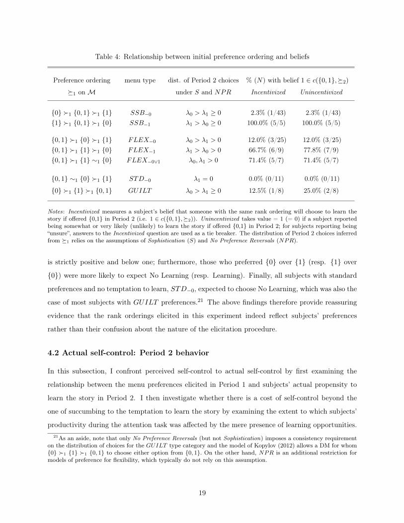
Table 4: Relationship between initial preference ordering and beliefs
Preference ordering menu type dist. of Period 2 choices % (N) with belief 1 2 c({0, 1},⌫2)
⌫1 on M under S and NPR Incentivized Unincentivized
{0} �1 {0, 1} �1 {1} SSB�0 �0 > �1 � 0 2.3% (1/43) 2.3% (1/43){1} �1 {0, 1} �1 {0} SSB�1 �1 > �0 � 0 100.0% (5/5) 100.0% (5/5)
{0, 1} �1 {0} �1 {1} FLEX�0 �0 > �1 > 0 12.0% (3/25) 12.0% (3/25){0, 1} �1 {1} �1 {0} FLEX�1 �1 > �0 > 0 66.7% (6/9) 77.8% (7/9){0, 1} �1 {1} ⇠1 {0} FLEX�0_1 �0,�1 > 0 71.4% (5/7) 71.4% (5/7)
{0, 1} ⇠1 {0} �1 {1} STD�0 �1 = 0 0.0% (0/11) 0.0% (0/11)
{0} �1 {1} �1 {0, 1} GUILT �0 > �1 � 0 12.5% (1/8) 25.0% (2/8)
Notes: Incentivized measures a subject’s belief that someone with the same rank ordering will choose to learn thestory if offered {0,1} in Period 2 (i.e. 1 2 c({0, 1},⌫2)). Unincentivized takes value = 1 (= 0) if a subject reportedbeing somewhat or very likely (unlikely) to learn the story if offered {0,1} in Period 2; for subjects reporting being“unsure”, answers to the Incentivized question are used as a tie breaker. The distribution of Period 2 choices inferredfrom ⌫1 relies on the assumptions of Sophistication (S) and No Preference Reversals (NPR).
is strictly positive and below one; furthermore, those who preferred {0} over {1} (resp. {1} over
{0}) were more likely to expect No Learning (resp. Learning). Finally, all subjects with standard
preferences and no temptation to learn, STD�0, expected to choose No Learning, which was also the
case of most subjects with GUILT preferences.21 The above findings therefore provide reassuring
evidence that the rank orderings elicited in this experiment indeed reflect subjects’ preferences
rather than their confusion about the nature of the elicitation procedure.
4.2 Actual self-control: Period 2 behavior
In this subsection, I confront perceived self-control to actual self-control by first examining the
relationship between the menu preferences elicited in Period 1 and subjects’ actual propensity to
learn the story in Period 2. I then investigate whether there is a cost of self-control beyond the
one of succumbing to the temptation to learn the story by examining the extent to which subjects’
productivity during the attention task was affected by the mere presence of learning opportunities.21As an aside, note that only No Preference Reversals (but not Sophistication) imposes a consistency requirement
on the distribution of choices for the GUILT type category and the model of Kopylov (2012) allows a DM for whom{0} �1 {1} �1 {0, 1} to choose either option from {0, 1}. On the other hand, NPR is an additional restriction formodels of preference for flexibility, which typically do not rely on this assumption.
19

4.2.1 Link between menu preferences and propensity to learn in Period 2
Out of the 120 subjects, 87 were asked to make a choice from the flexible menu {0, 1}; of the
remaining subjects, 29 received menu {0}, which removed all learning opportunities, while the last
4 subjects were assigned to learn the story for sure by receiving menu {1}. The analysis of this
subsection focuses on the 87 subjects who were offered to make a choice from {0, 1}.
Overall, 18.4% (16/87) of the subjects assigned {0, 1} chose to read the story at some point
during the attention task, with some heterogeneity in the timing of learning (see OA-C for learning
dynamics). For both of the classifications presented earlier, Figure 2 shows the proportion of subjects
who chose to learn the story during the task as a function of their menu preferences; as a benchmark,
actual learning is contrasted with subjects’ expectations of learning.
Figure 2: Learning expectations (incentivized) versus actual learning by menu type
Notes: “fraction who expected Learning” refers to the proportion of subjects who guessed that someone with the samerank ordering as them would choose to learn the story if offered {0,1}; patterns are very similar for the unincentivizedbelief measure (see OA Fig.10). Means were computed for each menu type using the classifications presented in Table1 (for top panel) and Table 3 (for bottom panel). See OA-D.2 for the number of observations in each menu typecategory (N � 4 in each bin).
As is immediately apparent from the figure, there is a lot of heterogeneity in the propensity to
learn the story across types and this observed heterogeneity is fairly consistent with what would be
expected under the restrictions of Sophistication and No Preference Reversals (see column 3 Table
20

4). In line with No Preference Reversals, subjects with preference {1} �1 {0} (such as SSB�1 and
FLEX�1) were significantly more likely to choose Learning than those with preference {0} �1 {1}
(such as SSB�0 and FLEX�0), although No Learning remained the most popular option even
among the former category.22 Of the 7 menu types, only FLEX�1 violates No Preference Reversals
(i.e. {1} �1 {0} implies �1 > �0), with a significantly higher proportion of subjects who chose not
to learn the story, while only STD�0 shows a minor departure from Sophistication, with a strictly
positive fraction of subjects who chose to learn the story. Importantly, the fraction of subjects with
self-control preferences who read the story is almost zero: of the 27 (16) subjects classified as SSB�0
in the initial (WTP ) classification, only one subject chose to learn. The pattern of behavior of the
SSB�0 subjects is also very consistent with their ex ante beliefs about their propensity to learn the
story. In other words, perceived self-control almost entirely translated into actual self-control, as
would be expected under Sophistication.
This unique combination of data on menu preferences, beliefs about Period 2 behavior and actual
Period 2 behavior provides a way to disentangle the theory of costly self-control of GP 2001 from
other theories of temptation. In the next table, I contrast the data with the predictions made by four
classes of temptation models under the assumption of sophisticated behavior. To make comparisons,
I look at the subset of 54 subjects who ex ante preferred not to learn the story but expressed being
tempted by it (i.e. for whom {0} �1 {1} and {0} �1 {0, 1}); among them, 35 made a choice
from {0, 1} in Period 2.23 The first class of models corresponds to standard models of dynamic
inconsistency with no uncertainty (Strotz [1956], Laibson [1997], O’Donoghue and Rabin [1999]).
As discussed in Section 2.2, present-biased agents who are sophisticated will choose to restrict their
choice set if and only if they expect to succumb to temptation. The next two classes are deterministic
models of costly self-control à la Gul and Pesendorfer (2001) and models of random indulgence in
which temptation is uncertain so that the DM only succumbs with probability p (Bénabou and
Pycia [2002], Chatterjee and Krishna [2009], Eliaz and Spiegler [2006], Duflo et al. [2011]). As
explained in Section 2.2, both classes of models can rationalize the ordering {0} �1 {0, 1} �1 {1},
but models of random of indulgence also predict a strictly positive probability of giving in. Finally,
the model of Kopylov (2012), which nests GP 2001 as a special case, can rationalize a form of
temptation induced by guilt or fear of making the wrong choice (see OA-D.3).22For the classification based on the initial rank ordering, 40.0% of subjects with preference {1} �1 {0} chose
to learn compared to 9.4% of those with preference {0} �1 {1} (t-stat = 2.25, p = 0.039). For the alternativeclassification based on WTP , the corresponding numbers are 42.9% and 13.8% (t-stat = 2.02, p = 0.061).
23Results are presented for the classification based on the initial rank ordering; the corresponding results for theWTP classification can be found in OA-D.3 (Table 11).
21

Table 5: Explanatory power of existing temptation models
Temptation model menu preferences expected propensity actual propensityto learn �1 to learn ⇢1
Dynamic Inconsistency {0} �1 {0, 1} ⇠1 {1} �1 = 1 ⇢1 = 1
(Strotz preferences)
Costly Self-Control {0} �1 {0, 1} �1 {1} �1 = 0 ⇢1 = 0
(GP 2001)
Random Indulgence {0} �1 {0, 1} �1 {1} �1 2 (0, 1) ⇢1 2 (0, 1)
(Stochastic Dual-Self models)
Temptation with Guilt {0} �1 {1} �1 {0, 1} �1 2 {0, 1} ⇢1 2 {0, 1}(Kopylov 2012)
Observed {0} �1 {0, 1} �1 {1} �1 = 0.04 ⇢1 = 0.09
for 79.6% (43/54) (2/54) (3/35)
Notes: Predictions and findings for the set of 54 subjects for whom {0} �1 {1} and {0} �1 {0, 1} according to theinitial rank ordering classification. Observed frequency �1 = 0.04 corresponds to the proportion of tempted subjectswho predicted that someone with the same ranking would learn the story and ⇢1 = 0.09 is the fraction of temptedsubjects who indeed learned the story.
As can be seen from the table, the only two theories consistent with the data as a whole are
those of costly self-control and random indulgence. However, for the latter to rationalize observed
behavior, the (perceived) probability of indulgence would have to be extremely low. In particular,
as previously shown, among the set of subjects with menu preferences {0} �1 {0, 1} �1 {1}, this
probability would have to be very close to zero (see Table 4 & Figure 2), thus making temptation
uncertainty a less compelling rationalization than costly self-control. The next findings provide
further evidence in favor of the theory of costly self-control.
4.2.2 Is there a cost of self-control?
Even though relatively few subjects end up learning the story, the GP model suggests that resisting
temptation may involve psychic costs, despite remaining silent about the nature of those costs. One
indirect way to test for the presence of self-control costs is to measure their impact on productivity.
Indeed, if self-control has to be exercised in order to avoid thinking about the possibility to learn
the story and entirely focus on the task, then subjects’ task performance should be higher when
22

all learning opportunities are removed. In other words, subjects should have a higher productivity
when assigned the commitment menu {0} rather than the flexible menu {0, 1}. Figure 3 shows
the percentage of subjects with a perfect score of 5 correct answers (left panel) and the average
number of correct answers (right panel) depending on the menu assigned (see OA-C.2 for additional
information on the distribution of productivities).
Figure 3: Productivity and menu assignment
Notes: % with perfect score refers to the percentage of subjects who provided a correct answer for each of the 5prompts received during the attention task. N = 87 (resp. N = 29) for those assigned {0,1} (resp. {0}).
Subjects assigned {0} were almost 20 percentage points more likely to obtain a perfect score
than those who faced {0, 1} (p = 0.037, one-sided t-test); furthermore, they gave 0.4 more correct
answers on average (p = 0.048, one-sided t-test). However, Figure 3 does not present a purely
experimental comparison since assignment to {0} or {0, 1} is exogenous only conditional on the
initial rank ordering and WTP choices made by a subject, which influence his ex ante odds of
receiving a given menu. Table 8 in the Appendix presents the results of regressions that control
for the odds of being assigned each menu given a subject’s rank ordering and WTP decisions. The
above findings are robust to the inclusion of these controls in the full sample.24 Although these24On the other hand, the effect of being assigned {0, 1} instead of {0} is not significant on the subsample of
SSB�0 types, although the effect size is comparable to the one of the full sample; there is also no differential impactof exposure to {0, 1} for SSB�0 types relative to the other types (regression results in subsamples available uponrequest). At the same time, attention levels during the task appear to have been differentially impacted only forSSB�0 types, who report higher levels of distraction when exposed to {0, 1} rather than {0}; see OA-B.2.
23

results should be interpreted with caution, they appear to be consistent with a large literature in
psychology, which proposes that willpower is a limited resource and shows that prior acts of self-
restraint such as resisting tempting food may lead to a subsequent breakdown of self-control on
cognitively challenging tasks (Baumeister et al. [1998], Vohs and Heatherton [2000], Baumeister
and Vohs [2003]).
5. Conclusion
In this paper, I propose a new experimental method designed to identify and document costly self-
control. This method is grounded in the theory of Gul and Pesendorfer (2001), which captures the
notions of temptation and self-control through the decision maker’s preferences over a set of menus.
Contrary to the more popular model of present bias, which can only rationalize overwhelming
temptation, GP 2001 suggests that there may be hidden costs to resisting tempting alternatives,
even if those alternatives are resisted eventually.
To measure the prevalence of self-control types, I conduct a laboratory experiment in which
subjects faced the temptation to forfeit money in order to learn a sensational story while performing
a mundane task. The identification strategy relies on a two-step procedure. First, I elicit subjects’
preferences over a set of menus, which either did or did not allow access to the story during the
task. Second, I implement subjects’ menu preferences using a probabilistic implementation rule.
This mechanism allows me to observe the behavior of subjects who faced the flexibility of choice,
yet preferred commitment and to contrast perceived self-control with actual self-control. With
this rich dataset containing menu preferences, beliefs about ex post choice and realized ex post
choice, I can assess the explanatory power of the GP model relative to other temptation models.
To my knowledge, this is the first experimental design allowing to disentangle various theories of
temptation.
In this specific setting, between a quarter and a third of subjects can be classified as self-control
types according to their menu preferences, a proportion which is 3 to 4 times higher than what
would be observed if subjects had picked a rank ordering at random. Consistent with their menu
preferences, almost all self-control types predicted that they would resist the temptation to learn the
story in the absence of commitment. Furthermore, perceived self-control, as measured by subjects’
menu preferences and anticipated choices, almost entirely coincides with actual self-control when
facing the choice: while 18% of subjects read the story when offered the choice, all but one subject
24

with self-control preferences succumbed to the temptation. Finally, although relatively few subjects
chose to learn the story, the mere presence of learning opportunities seems to have negatively
impacted productivity in the whole sample.
These results are obviously specific to the particular environment considered in this paper and
may not extend to different settings. In this specific environment, subjects faced relatively little
uncertainty since the attention task was straightforward and all decisions (Period 1 & 2) occurred
within a single session. These features of the experiment could explain why demand for flexibility was
relatively low and subjects correctly anticipated that they would resist temptation. An important
area of future work is therefore to understand how the prevalence of self-control types may vary
across decision environments.
Yet, if they generalized to other settings, these findings would have important implications for the
design of policies aiming to reduce the welfare costs of temptation. Although not every customer
ends up purchasing the unhealthy snacks readily available at cashier counters, the above results
suggest that there are hidden costs to resisting those environmental cues, with potential collateral
damages such as a reduced focus on some other tasks. As a consequence, customers’ welfare could
greatly increase if those tempting options were removed from immediate sight.
25
Appendix
Figure 4: Distribution of WTP by condition and comparison of ranks
Notes: Each histogram shows the proportion of subjects who are willing to pay to replace one menu with the menuranked just above for each payment value, ranging from $0.01 to $0.50 in the dollar WTP condition and from 1 to 10minutes in the time WTP condition. The distributions are shown separately for top versus second choice and secondversus last choice.
Figure 5: Relationship between belief about other and belief about oneself
26
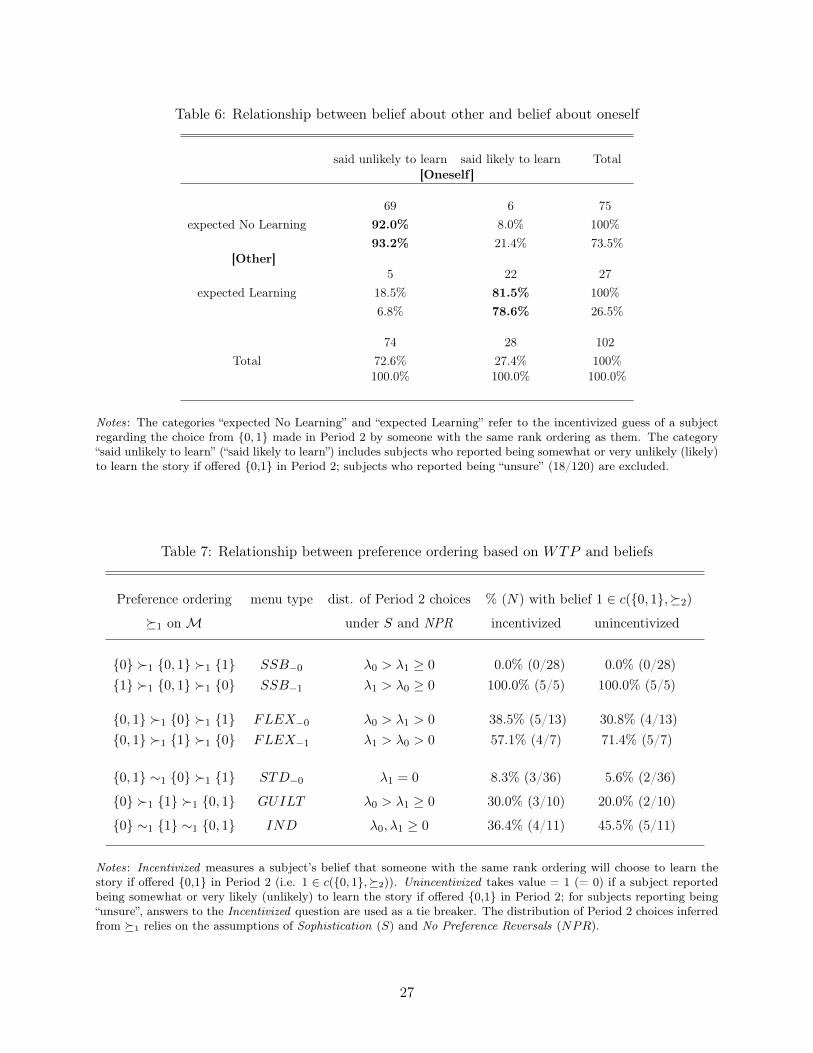
Table 6: Relationship between belief about other and belief about oneself
said unlikely to learn said likely to learn Total[Oneself ]
69 6 75expected No Learning 92.0% 8.0% 100%
93.2% 21.4% 73.5%[Other]
5 22 27expected Learning 18.5% 81.5% 100%
6.8% 78.6% 26.5%
74 28 102Total 72.6% 27.4% 100%
100.0% 100.0% 100.0%
Notes: The categories “expected No Learning” and “expected Learning” refer to the incentivized guess of a subjectregarding the choice from {0, 1} made in Period 2 by someone with the same rank ordering as them. The category“said unlikely to learn” (“said likely to learn”) includes subjects who reported being somewhat or very unlikely (likely)to learn the story if offered {0,1} in Period 2; subjects who reported being “unsure” (18/120) are excluded.
Table 7: Relationship between preference ordering based on WTP and beliefs
Preference ordering menu type dist. of Period 2 choices % (N) with belief 1 2 c({0, 1},⌫2)
⌫1 on M under S and NPR incentivized unincentivized
{0} �1 {0, 1} �1 {1} SSB�0 �0 > �1 � 0 0.0% (0/28) 0.0% (0/28){1} �1 {0, 1} �1 {0} SSB�1 �1 > �0 � 0 100.0% (5/5) 100.0% (5/5)
{0, 1} �1 {0} �1 {1} FLEX�0 �0 > �1 > 0 38.5% (5/13) 30.8% (4/13){0, 1} �1 {1} �1 {0} FLEX�1 �1 > �0 > 0 57.1% (4/7) 71.4% (5/7)
{0, 1} ⇠1 {0} �1 {1} STD�0 �1 = 0 8.3% (3/36) 5.6% (2/36)
{0} �1 {1} �1 {0, 1} GUILT �0 > �1 � 0 30.0% (3/10) 20.0% (2/10)
{0} ⇠1 {1} ⇠1 {0, 1} IND �0,�1 � 0 36.4% (4/11) 45.5% (5/11)
Notes: Incentivized measures a subject’s belief that someone with the same rank ordering will choose to learn thestory if offered {0,1} in Period 2 (i.e. 1 2 c({0, 1},⌫2)). Unincentivized takes value = 1 (= 0) if a subject reportedbeing somewhat or very likely (unlikely) to learn the story if offered {0,1} in Period 2; for subjects reporting being“unsure”, answers to the Incentivized question are used as a tie breaker. The distribution of Period 2 choices inferredfrom ⌫1 relies on the assumptions of Sophistication (S) and No Preference Reversals (NPR).
27

Table 8: Effect of flexible menu on productivity
Received perfect score Number of correct answers
(1) (2) (3) (4)
assigned {0,1} -0.22** -0.19* -0.43* -0.39*(0.10) (0.11) (0.23) (0.23)
assigned {1} -0.34 -0.26 -0.70 -0.54(0.26) (0.26) (0.57) (0.57)
odds of {0} 1.30** 2.09*(0.55) (1.20)
odds of {0,1} 1.06* 2.12(0.61) (1.34)
Observations 120 120 120 120
Mean dependent variable 0.37 0.37 3.93 3.93
Notes: Columns (1) & (2) are linear probability models where the dependent variable Received perfect score is equalto 1 if the subject correctly answered all 5 prompts; probit models give almost identical results. Session fixed effectsincluded in all regressions. * and ** refer to p < 0.1 and < 0.05.
References
[1] Acland, Daniel. J. and Matthew Levy (2015), “Naiveté, Projection Bias, and Habit Formation
in Gym Attendance”, Management Science, 61(1): 146–160.
[2] Ahn, David and Todd Sarver (2013), “Preference for Flexibility and Random Choice”, Econo-
metrica, 81(1): 341–361.
[3] Ameriks, John, Andrew Caplin, John Leahy and Tom Tyler (2007), “Measuring self-control
problems”, American Economic Review, 97: 966–972.
[4] Ashraf, Nava, Dean Karlan, and Wesley Yin (2006), “Tying Odysseus to the Mast: Evidence
from a Commitment Savings Product in the Philippines,” Quarterly Journal of Economics,
121(1): 635–672.
[5] Augenblick, Ned, Muriel Niederle, and Charles Sprenger (2015), “Working over Time: Dynamic
Inconsistency in Real Effort Tasks,” Quarterly Journal of Economics, 130(3): 1067–1115.
[6] Augenblick, Ned and Matthew Rabin (2015), “An Experiment on Time Preference and Mispre-
diction in Unpleasant Tasks”, working paper.
28

[7] Baumeister, Roy, Ellen Bratslavsky, Mark Muraven and Dianne Tice (1998), Journal of Per-
sonality and Social Psychology, 74(5): 1252-1265.
[8] Baumeister, Roy and Kathleen Vohs (2003), “Willpower, Choice, and Self-Control” in Loewen-
stein, George, Daniel Read and Roy F. Baumeister, eds. Time and Decision. New York: Russell
Sage Foundation.
[9] Bénabou, Roland and Marek Pycia (2002), “Dynamic Inconsistency and Self-Control: A Plan-
ner–Doer Interpretation,” Economic Letters, 77, 419–424.
[10] Bonein, Aurélie and Laurent Denant-Boemont (2015), “Self-Control, Commitment and Peer
Pressure: A Laboratory Experiment,” Experimental Economics, forthcoming.
[11] Bucciol, Alessandro, Daniel Houser and Marco Piovesan (2013), “Temptation at Work,” PLoS
ONE, 8(1): 1–5.
[12] Butler, Jeffrey, Paola Giuliano and Luigi Guiso (2015), “Trust, Values and False Consensus”,
International Economic Review, 56 (3): 889-915.
[13] Chatterjee, Kalyan and R. Vijay Krishna (2009), “A “Dual Self” Representation for Stochastic
Temptation”, American Economic Journal: Microeconomics, 1(2): 148-67.
[14] Dean, Mark and John McNeill (2015), “Preference for Flexibility and Random Choice: an
Experimental Analysis”, working paper.
[15] Dekel, Eddie and Barton Lipman (2012), “Costly Self-Control and Random Self-Indulgence”,
Econometrica, 80(3): 1271–1302.
[16] DeYoung, Colin, Jordan Peterson and Lena Quilty (2007), “Between Facets and Domains: 10
Aspects of the Big Five”, Journal of Personality and Social Psychology, 93(5): 880–896.
[17] Duflo, Esther, Michael Kremer and Jonathan Robinson (2011), “Nudging Farmers to Use Fer-
tilizer: Evidence from Kenya,” American Economic Review, 101(6): 2350–2390.
[18] Dunbar, Robin (2004), “Gossip in Evolutionary Perspective”, Review of General Psychology,
8(2): 100–110.
[19] Eliaz, Kfir and Ran Spiegler (2006), “Contracting with Diversely Naive Agents,” Review of
Economic Studies, 72, 689–714.
29

[20] Ellingsen, Tore and Magnus Johannesson (2009), “Time Is Not Money”, Journal of Economic
Behavior and Organization, 72(1): 96–102.
[21] Ellingsen, Tore, Magnus Johannesson, Sigve Tjøtta and Gaute Torsvik (2010), “Testing Guilt
Aversion”, Games and Economic Behavior, 68(1): 95–107.
[22] Giné, Xavier, Dean Karlan, and Jonathan Zinman (2010), “Put Your Money Where Your Butt
Is: A Commitment Contract for Smoking Cessation,” American Economic Journal: Applied
Economics, 2(4): 213–35.
[23] Gul, Faruk and Wolfgang Pesendorfer (2001), “Temptation and Self-Control,” Econometrica,
69(6): 1403–1435.
[24] Houser, Daniel, Daniel Schunk, Joachim Winter and Erte Xiao (2010), “Temptation and Com-
mitment in the Laboratory”, working paper.
[25] John, Anett (2015), “When Commitment Fails - Evidence from a Regular Saver Product in the
Philippines,” EOPP Discussion Papers 55, London School of Economics.
[26] Kopylov, Igor (2012), “Perfectionism and Choice,” Econometrica, 80(5): 1819–1843.
[27] Kreps, David (1979), “A Representation Theorem for Preference for Flexibility”, Econometrica,
47: 565–576.
[28] Krusell, Per, Burhanettin Kuruşçu and Anthony A. Smith Jr. (2010), “Temptation and Taxa-
tion”, Econometrica, 78(6), 2063–2084.
[29] Krusell, Per, Burhanettin Kuruşçu and Anthony A. Smith Jr. (2007), “Temptation and Taxa-
tion”, working paper, June 2007.
[30] Laibson, David (1997), “Golden Eggs and Hyperbolic Discounting,” Quarterly Journal of Eco-
nomics, 112(2): 443–477.
[31] Lipman, Barton and Wolfgang Pesendorfer (2013), “Temptation,” in Acemoglu, Arellano, and
Dekel, eds., Advances in Economics and Econometrics: Tenth World Congress, Volume 1,
Cambridge University Press.
[32] Litman, Jordan and Charles Spielberger (2003), “Measuring Epistemic Curiosity and Its Diver-
sive and Specific Components”, Journal of Personality Assessment, 80(1): 75–86.
30

[33] Litman, Jordan and Tiffany Jimerson (2004), “The Measurement of Curiosity As a Feeling of
Deprivation”, Journal of Personality Assessment, 82(2): 147–157
[34] Milkman, Katherine, Julia Minson, and Kevin Volpp (2014), “Holding the Hunger Games
Hostage at the Gym: An Evaluation of Temptation Bundling,” Management Science, 60(2):
283–299.
[35] O’Donoghue, Ted and Matthew Rabin (1999), “Doing it Now or Later,” American Economic
Review, 89(1): 103–124.
[36] Ross, Lee, David Greene, and Pamela House (1977), “The False Consensus Phenomenon: An
Attributional Bias in Self-Perception and Social Perception Processes”, Journal of Experimental
Social Psychology, 13(3): 279–301.
[37] Rubinstein, Ariel and Yuval Salant (2015), “ “Isn’t everyone like me?” On the presence of
self-similarity in strategic interactions”, working paper.
[38] Sadoff, Sally, Anya Samek and Charles Sprenger (2015), “Dynamic Inconsistency in Food
Choice: Experimental Evidence from a Food Desert”, working paper.
[39] Schilbach, Frank (2015), “Alcohol and Self-Control: A Field Experiment in India”, working
paper.
[40] Strotz, Robert H. (1956), “Myopia and Inconsistency in Dynamic Utility Maximization,” Review
of Economic Studies, 23: 165–180.
[41] Toussaert, Séverine (2014), “Connecting commitment to self-control: evidence from a field
experiment with participants in a weight loss challenge”, working paper.
[42] Vohs, Kathleen and Todd Heatherton (2000), “Self-Regulatory Failure: A Resource-Depletion
Approach,” Psychological Science, 11: 249-254.
[43] Wong, Wei-Kang (2008), “How much time-inconsistency is there and does it matter? Evidence
on self-awareness, size, and effects”, Journal of Economic Behavior and Organization, 68, Issues
3–4: 645–656.
31