Embed Size (px)
Citation preview

ELECTRONIC DESIGN AUTOMATION FOR AN ENERGY-EFFICIENT COARSE-GRAIN RECONFIGURABLE FABRIC ARCHITECTURE
by
Justin Nathanial Stander
BS, University of Pittsburgh, 2005
Submitted to the Graduate Faculty of
the School of Engineering in partial fulfillment
of the requirements for the degree of
Master of Science
University of Pittsburgh
2007

ii
UNIVERSITY OF PITTSBURGH
SCHOOL OF ENGINEERING
This thesis was presented
by
Justin Nathanial Stander
It was defended on
July 5th, 2007
and approved by
Jun Yang, Assistant Professor, Departmental of Electrical and Computer Engineering
Tom Cain, Professor, Departmental of Electrical and Computer Engineering
Thesis Advisor: Alex K. Jones, Assistant Professor, Departmental of Electrical and Computer
Engineering

iii
Copyright © by Justin Nathanial Stander
2007

iv
In the past those looking to accelerate computationally intensive applications through hardware
implementations have had relatively few target platforms to choose from, each with wildly
opposing benefits and drawbacks. The SuperCISC Energy-Efficient Coarse-Grain
Reconfigurable Fabric provides an ultra-low power alternative to field-programmable gate array
(FPGA) devices and application specific integrated circuits (ASICs). The proposed Fabric
combines the reconfigurable nature and manageable Computer-Aided Design (CAD) flow of
FPGAs with power and energy characteristic similar to those of an ASIC.
This thesis establishes the design flow and explores issues central to the design space
exploration of the SuperCISC Reconfigurable Fabric Project. The Fabric Interconnect Model
specification facilitates rapid design space exploration for a range of Fabric Models. Significant
effort was put into the development of the Heuristic Mapper which automates the problem of
programming the Fabric to perform the desired hardware function. Coupled with additional
automation the Mapper allows for conversion of C-code specified application kernels into Fabric
Configurations. The FIMFabricPrinter automates the verification, simulation, statistics
gathering, and visualization of these Fabric Configurations. Results show the Fabric achieving
power improvements of 68X to 369X, and energy improvements of 38X to 127X over the same
benchmarks performed on an FPGA device.
ELECTRONIC DESIGN AUTOMATION FOR AN ENERGY-EFFICIENT COARSE-GRAIN RECONFIGURABLE FABRIC ARCHITECTURE
Justin Nathanial Stander, M.S.
University of Pittsburgh, 2007

v
TABLE OF CONTENTS
PREFACE.................................................................................................................................. XIII
1.0 INTRODUCTION ......................................................................................................... 1
2.0 RELATED WORK & BACKGROUND....................................................................... 7
2.1 COARSE GRAIN FABRIC ARCHITECTURES................................................. 7
2.2 SUPERCISC ARCHITECTURE........................................................................... 9
2.2.1 SuperCISC Automated Flow ........................................................................ 10
2.2.2 Example Hardware Function ........................................................................ 11
3.0 HEURISTIC BASED FABRIC MAPPER .................................................................. 17
3.1 PREPROCESSING.............................................................................................. 19
3.2 ROW ASSIGNMENTS....................................................................................... 22
3.3 COLUMN ASSIGNMENTS............................................................................... 27
3.3.1 Initial Heuristic Column Assignment ........................................................... 30
3.3.2 Refining the Heuristic ................................................................................... 35
3.3.3 Optimizing Child Dependency: Potential Linked Placement Values ........... 35
3.3.4 Optimizing Child Dependency: Potential Child Placement Values ............. 36
3.3.5 Dealing with unary operations ...................................................................... 37
3.3.6 Picking Next Operation to Map .................................................................... 37
3.3.7 Force System................................................................................................. 38

vi
3.3.8 Grandchild Dependency................................................................................ 39
3.3.9 Centering....................................................................................................... 40
3.4 FINAL HEURISTIC............................................................................................ 41
3.5 MAPPING REPRESENTATION ....................................................................... 43
3.6 MAPPING TO DEDICATED PASSGATES...................................................... 43
4.0 FABRIC INTERCONNECT MODEL (FIM).............................................................. 44
4.1 EXTENSIBLE MARKUP LANGUAGE (XML) ............................................... 44
4.2 FIM DEFINED .................................................................................................... 45
4.3 SVG VISUALIZATION ..................................................................................... 50
4.4 FIM VERIFICATION ......................................................................................... 51
4.5 FIM FRONT-END INTERFACE........................................................................ 53
5.0 VERIFICATION AND CONFIGURATION .............................................................. 54
5.1 PARAMETERS AND INPUTS .......................................................................... 54
5.2 VERIFICATION AGAINST FIM....................................................................... 56
5.3 DYNAMICALLY DETERMINING MULTIPLEXER CONTROL SIGNALS 56
5.4 BUILDING CONFIGURATION FILES ............................................................ 57
5.5 GENERATING STATISTICS ........................................................................... 58
5.6 GENERATING VISUALIZATION.................................................................... 58
6.0 PERFORMANCE RESULTS...................................................................................... 60
6.1 FABRIC INTERCONNECT MODELS.............................................................. 61
6.1.1 8:1-based Fabric Models............................................................................... 61
6.1.2 4:1-based Fabric Models............................................................................... 62
6.1.3 3553:1-based Fabric Models......................................................................... 64

vii
6.2 BENCHMARK KERNELS................................................................................. 64
6.3 SOLUTION IMPROVEMENT DURING DEVELOPMENT OF HEURISTIC 66
6.4 COMPARING MAPPING TECHNIQUES ........................................................ 68
6.4.1 Runtime Comparison .................................................................................... 69
6.4.2 Mapping Size Comparison............................................................................ 70
6.4.3 Power / Energy Comparisons........................................................................ 70
6.4.4 Delay Comparison ........................................................................................ 73
6.4.5 Analysis......................................................................................................... 75
6.5 HEURISTIC MAPPER RESULTS ON A VARIETY OF FABRIC MODELS. 75
6.5.1 Integrated Constants Results......................................................................... 76
6.5.2 Dedicated Passgates Results ......................................................................... 78
6.6 COMPARING FABRIC VS CURRENT HARDWARE TECHNOLOGIES..... 80
6.7 COMPARING HEURISTIC AGAINST AS SOON AS POSSIBLE ................. 82
7.0 CONCLUSION............................................................................................................ 84
7.1 FUTURE DIRECTIONS..................................................................................... 85
7.1.1 Global Lookahead Information..................................................................... 86
7.1.2 Global Lookahead Heuristic For First Row Mapping .................................. 86
7.1.3 Handling Heterogeneous Fabric Models ...................................................... 87
APPENDIX A. FABRIC INTERCONNECT MODEL FILES.................................................... 89
APPENDIX B. XML SCHEMA FOR FABRIC INTERCONNECT MODEL ........................... 99
BIBLIOGRAPHY....................................................................................................................... 102

viii
LIST OF TABLES
1: The Complete FIM specification: Elements and Attributes. .................................................... 48
2: Benchmark sizes ....................................................................................................................... 66
3: Heuristic Mapper Versions Summary....................................................................................... 67
4: Heuristic Versions: Processing time & added rows for 5:1-based Standard FIM. ................... 67
5: CPU Runtime (seconds) of each mapper for 3553:1, 4:1, 5:1 & 8:1 standard FIMs. .............. 69
6: Rows added by each mapper for 3553:1, 4:1, 5:1 & 8:1 standard FIMs. ................................. 70
7: Power (mW) of fabric mappings for 3553:1, 4:1, 5:1, & 8:1 standard FIMs across methods. 71
8: Energy (pJ) of fabric mapping for 3553:1, 4:1, 5:1, & 8:1 standard FIMs across methods. .... 71
9: Total delay (ns) of mappings when implemented onto the Fabric. .......................................... 74
10: FIM variations, each could be coupled with any level of interconnect (8:1, 5:1, etc)............ 76
11: Rows added to solve 8:1, 5:1, and 3553:1 Std & IC FIMs using Heuristic Mapper. ............ 77
12: Rows added to solve 8:1, 6:1, and 5:1 Standard & Dedicated Passgate FIMs ....................... 79
13: Power (mW) usage of benchmark implementations on ASIC, Fabric, FPGA, and XScale. .. 81
14: Energy (pJ) usage of benchmark implementations on ASIC, Fabric, FPGA, and XScale..... 81
15: Energy (pJ) comparison ASAP Schedule Solutions VS. Heuristic Mapper Solutions........... 83

ix
LIST OF FIGURES
1: Amdahl's Law for total speedup of an application. .................................................................... 2
2: High-Level Fabric Model. .......................................................................................................... 3
3: Multiplexer based interconnect stripe......................................................................................... 4
4: Design space exploration flow of the fabric model. ................................................................... 5
5: SuperCISC Architecture ........................................................................................................... 10
6: SuperCISC Hardware Function Generation Flow. ................................................................... 11
7: Sobel Edge Detection Hardware Function C Source Code. ..................................................... 11
8: Sobel CDFG showing Control Flow and Basic Blocks............................................................ 12
9: Sobel Super Data Flow Graph. ................................................................................................. 14
10: VHDL for 32 bit subtract found in Sobel SDFG. ................................................................... 15
11: Entity and port declarations for Sobel SDFG. ........................................................................ 16
12: Overall Heuristic Mapper Flow. ............................................................................................. 18
13: Before/After Replacing converts and negate operations in an SDFG. ................................... 19
14: Before/After Integrating constant values into SDFG operations............................................ 20
15: SDFG with ALAP annotations. .............................................................................................. 21
16: Before/After Row alignment state of Heuristic Mapper......................................................... 24
17: Pseudocode for row-alignment section of Heuristic Mapper. ................................................ 26
18: Example Parent Dependency Window construction assuming 4:1 based interconnect. ........ 28

x
19: Example of Child Dependency Window (CDW) construction. ............................................. 29
20: Example Functional Unit Desirability (FUD) construction.................................................... 30
21: Initial Heuristic column placement pseudocode..................................................................... 32
22: Before/After Dynamically delaying an operation during mapping. ....................................... 34
23: Example of finding Potential Linked Placement (PLP) Values. ............................................ 36
24: Example of Building the Grandchild Dependency Window (GDW). .................................... 40
25: Final Heuristic Column Assignments Pseudocode................................................................. 42
26: A short CD catalogue written using XML.............................................................................. 45
27: FIM Code for an ALU Definition........................................................................................... 46
28: FIM Pattern Section for a standard 8:1 multiplexer based model. ......................................... 47
29: FIM Pattern Code for a 50% Dedicated Passgates, half 8:1 & half 4:1 interconnect............. 49
30: Portion of a rendered SVG file for FIM shown in Figure 20. ................................................ 50
31: XML Schema Definition (XSD) for Catalogue of CDs XML file shown in Figure 26. ........ 52
32: FIM Fabric Printer Parameters. .............................................................................................. 55
33: Equation to determine output rows when using outputmux fabric feature............................. 55
34: Example of control signal generation using 4:1 multiplexer. ................................................. 57
35 : SVG representation of Sobel mapping on 8:1-based FIM..................................................... 59
36: Visualization of 8:1-based Interconnect. ................................................................................ 61
37: SVG Visualization of 4:1-based Interconnect. ....................................................................... 62
38: SVG Visualization of 5:1-based Interconnect. ....................................................................... 63
39: SVG Visualization of 6:1-based Interconnect. ....................................................................... 63
40: SVG Visualization of 3553:1-based Interconnect. ................................................................. 64
41: Energy Comparison of 8:1 standard FIM across mappers...................................................... 72

xi
42: Energy Comparison of 5:1 standard FIM across mappers...................................................... 73
43: Comparing Average runtime for each Mapper/FIM combination......................................... 74
44: Energy Comparison between Standard and Integrated Constant FIMs.................................. 78
45: Energy Comparison between 8:1, 5:1, Standard and Dedicated Passgates FIMs................... 79
46: Energy Comparison between hardware technologies............................................................. 82

xii
LIST OF ACRONYMS
1. ALAP As Late as possible
2. ALU Arithmetic Logic Unit
3. ASIC Application Specific Integrated Circuit
4. BB Basic Block
5. CDFG Control Data Flow Graph
6. CISC Complex Instruction Set Computing
7. CP Constraint Programming
8. DP Dedicated Passgates
9. FIM Fabric Interconnect Model
10. FPGA Field Programmable Gate Array
11. FTU Fabric Topological Unit
12. FUD Functional Unit Desirability
13. IC Integrated Constants
14. MILP Mixed Integer Linear Program
15. SDFG Super Data Flow Graph
16. SVG Scalable Vector Graphics
17. VHDL VHSIC Hardware Description Language
18. XML Extensible Markup Language

xiii
PREFACE
I would like to express my appreciation of the hard work and efforts of all the present and past
members of the SuperCISC and Fabric research teams especially Josh Lucas, Josh Fazekas,
Gayatri Mehta, Colin Ihrig, Mustafa Baz, and Professor Brady Hunsaker. Many thanks go to my
advisor Dr. Alex Jones for his continued support over the last few years. I would also like to
thank Dr. Tom Cain and Dr. Jun Yang for serving on my master’s thesis committee.

1
1.0 INTRODUCTION
In order to utilize a reconfigurable device such as a Coarse-Grain reconfigurable Fabric a method
must be devised in order to configure the device to perform a desired application. Additionally
in order for this method to allow for variations and changes to the Fabric architecture it must be
extensible and parameterizable. This thesis addresses this problem through the introduction of a
C to Fabric design flow featuring a Heuristic Mapper which incorporates a method of Fabric
Modeling to handle different Fabric variants as well as a set of visualization, verification, and
testing support tools.
Contributions:
1. Heuristic Mapper for solving Fabric Configuration
2. Fabric Interconnect Model (FIM) facilitating rapid design space exploration
3. Visualization & Verification of Fabric Mappings
4. Support for simulation and power/performance analysis of Fabric hardware
In recent years system and application developers have realized large speedups with the
use of processors equipped with application specific auxiliary hardware. In order to pursue this
type of solution the application must first be broken down into hardware and software portions.
By placing into hardware the sections of the application which take up a large portion of overall
execution time a significant overall performance increase can be realized. Typically in these
types of applications a small portion of computationally intensive code (10% of the code) uses

2
up a large portion of the execution time (90% of time). The relationship between speedup of a
hardware portion in relation to the overall performance improvement is best represented by
Amdahl’s law (shown in Figure 1).
Speedup =
P: Portion of overall time spent in accelerated portion.
S: Speedup of accelerated portion.
Figure 1: Amdahl's Law for total speedup of an application.
Those looking to accelerate computationally intensive applications through hardware
implementations have had relatively few target platforms to choose from, each with wildly
opposing benefits and drawbacks. Modern day Application Specific Integrated Circuits (ASICs)
possess excellent power and performance characteristics. However they still invoke a large up-
front fabrication and development cost (non-recurring engineering cost) for each new chip
designed. In addition they require complex and expensive Computer Aided Design (CAD) tools
as well as long manufacturing times. Meanwhile solutions using highly flexible Field-
Programmable Gate Array (FPGA) devices are both fast and easy to develop. While highly
reprogrammable and able to support a wide variety of applications, FPGAs suffer from relatively
poor power and energy characteristics, making this route infeasible for many potential uses.

3
This thesis will demonstrate that a third way, specifically a reconfigurable low power
coarse-grain “Fabric” solution is both possible and competitive against FPGA and ASIC
implementations. While possessing the ease of development found in the FPGA world, the
Fabric uses dramatically less power, putting it close to the power and energy characteristics of an
ASIC solution. In particular this thesis will focus on the problems which arise from targeting
such a device and specifically the problem of finding a valid fabric configuration (“Mapping”)
which programs the device to perform a desired program.
Figure 2: High-Level Fabric Model.

4
A high level diagram of an ALU-homogeneous version of the Fabric is shown in Figure
2. Each fabric row consists of a number of Functional Units, each able to perform a set of
operations on their inputs. Most often these Functional Units are Arithmetic & Logic Units
(ALUs), although whether the fabric is homogeneous or a mix of ALUs with different
capabilities (heterogeneous) and units dedicated to specific functionality (ex: dedicated
passgates) is a decision to be determined by extensive design space exploration. In between each
fabric row lies a layer of multiplexer based interconnect (Figure 3) which determines the possible
connections that can be made between adjacent fabric rows. In order to program the Fabric a set
of control signals for each functional unit and interconnect multiplexer must be set properly
(fabric configuration).
Figure 3: Multiplexer based interconnect stripe.
In order to implement actual hardware functions onto the Fabric an automated Heuristic
“Mapper” was developed. The Heuristic Mapper creates a fabric configuration which performs
the desired hardware function by finding a valid placement of all operations which allows the
interconnect system to connect operations correctly. The Heuristic Mapper uses a two-tiered

5
top-down approach wherein operations are first assigned into fabric rows in a row-alignment
stage before the heuristic determines the fabric location to place each operation in during the
column-assignment stage. A detailed explanation of the heuristic and workings of the mapper
are found in Section 3.0 .
Figure 4 shows the design space exploration flow used for the Fabric. To facilitate
design space exploration and to provide a unified fabric description the Fabric Interconnect
Model (FIM) specification was developed. Designed with maximum versatility in mind the
model contains all information needed to describe any particular fabric model. Primarily this
consists of a full description of each Functional Unit as well as the interconnect stripe found
between each fabric row. A support library and other tools (such as visualization) were then
developed so that the FIM could be used by the entire suite of Fabric CAD tools. A full
description of the FIM is found in Section 4.0 .
Figure 4: Design space exploration flow of the fabric model.

6
After determining a valid mapping the proper control signals must be generated in order
to test and simulate the mapping. In order to avoid human-errors and automate the process a
verification tool, the FimFabricPrinter software application was developed. In addition to
generating the fabric configuration files for simulation the Printer also can verify a mapping
against the FIM file, this ensures that the Mapper is properly obeying the constraints of the
Fabric Model. Other features include creation of mapping visualization and verification files
which can be used during simulation to ensure the Fabric achieves the correct results. A full
description of the FimFabricPrinter tool is found in Section 5.0 .
Section 2.0 introduces related work and background information upon which this project
builds. Section 6.0 contains the results of running a set of benchmarks on a variety of Fabric
Models using the Heuristic Mapper as well as two alternative methods of mapping. A
comparison against ASIC and FPGA implementations is included. Lastly Section 8.0 discusses
potential future directions and provides a concluding summary of the project.

7
2.0 RELATED WORK & BACKGROUND
A short comparison between other coarse grain fabrics architectures and this project is included
to contrast the Fabric architecture against other projects in the same field of devices. A review of
material originally created for the SuperCISC architecture/compiler project[1,2] is included as
portions of the SuperCISC compiler flow have been incorporated into the C to Fabric design
flow discussed throughout this thesis. In particular this includes creation of Control and Data
Flow Graphs (CDFG), and a hardware predication method which allows for the creation of
“Super” Data Flow Graphs (SDFG).
2.1 COARSE GRAIN FABRIC ARCHITECTURES
Over the past several years, a tremendous amount of effort has been devoted to the area of
reconfigurable computing. Since fine-grained fabrics like FPGAs are not considered appropriate
for computationally intensive applications due to their poor power characteristics and significant
routing overhead, the area of reconfigurable computing stresses the development and use of
coarse-grained fabrics for computationally complex tasks. Many architectures have been
proposed and developed both in academia and industry during the last decade including
MATRIX, Garp, Chimaera, RaPiD, PipeRench, Elixent, XPP, and FPOA.

8
MATRIX (Multiple ALU architecture with Reconfigurable Interconnect eXperiment) [3]
is comprised of a two-dimensional array of identical 8-bit functional units with a configurable
network. Each functional unit consists of a 256x8-bit memory block, an 8-bit ALU and control
logic. The Garp [4], Chimaera [5] and SuperCISC [1] architectures combine a reconfigurable
computing device with a processor to perform hardware acceleration. RaPiD (Reconfigurable
Pipelined Datapath) [6,7], mainly intended for computation intensive applications, consists of a
linear array of application-specific function units. PipeRench [8,9] has a striped configuration and
is comprised of an interconnected network of configurable logic blocks and storage elements. It
consists of a set of physical pipeline stages called stripes and each stripe contains a set of
processing elements, register files and an interconnection network.
The Reconfigurable Algorithm Processor (RAP) from Elixent [10] is comprised of an
array of 4-bit ALUs and register/buffer blocks that can be cascaded to suit different data widths.
The ALUs are arranged in a chessboard-style array, alternating with adjacent switchboxes.
Pact XPP Technologies [11] proposed the XPP architecture which has a hierarchical
array of coarse-grained adaptive computing elements called Processing Array Elements (PAEs)
and a packet-oriented communication network. An XPP core is comprised of a rectangular array
of ALU-PAEs and RAM-PAEs with I/O.
MathStar [12] proposed Field Programmable Object Array (FPOA) which consists of a
2D array of Silicon Objects (SOs). Silicon Objects are 16-bit configurable machines such as
ALU, Multiply-Accumulate Unit or Register File. Both Silicon Object behavior and the
interconnection among Silicon Objects are field-programmable.
Unlike MATRIX whose basic functional unit consists of an 8-bit ALU and a SRAM, the
basic functional unit in the proposed Fabric (introduced in Section 1) is a coarse-grained ALU
9
having variable datawidth. There is no internal memory or storage element in the proposed
model. Unlike GARP and Chimaera the proposed Fabric uses an application domain tailored
hardware co-processor. Compared to RaPiD, which has small RAMs and registers to store data
and intermediate results, the proposed Fabric is purely combinational. The programmable
connections in the datapath interconnect in the proposed Fabric are modeled as multiplexers
somewhat similar to those in RaPiD. Unlike RAP who’s ALUs are arranged in a chessboard
style, the proposed fabric model has a striped configuration like that of PipeRench but without
register files. Compared to the XPP architecture which is comprised of a mixture of ALU-PAEs
and RAM-PAEs, the proposed fabric consists of only an array of ALUs with no memory
elements.
2.2 SUPERCISC ARCHITECTURE
The SuperCISC architecture[1] in Figure 5 shows a 4-way very long instruction word (VLIW)
core, surrounded by a series of hardware functions connected to the core via a shared register
file. The goal is to accelerate sections of code that use significant amounts of execution time by
converting these code sections into combinational hardware functions. In order to facilitate this
process an automated flow was developed which converts user designated C code sections into
synthesizable VHDL blocks, allowing them to be implemented as hardware functions.

10
Figure 5: SuperCISC Architecture
2.2.1 SuperCISC Automated Flow
Figure 6 shows the hardware function design flow that SuperCISC uses to create its hardware
functions. An application is first profiled to determine where hardware functions should be
created. After specifying each desired hardware block with pragma compiler directives the
SuperCISC compiler creates a Control-Data Flow Graph (CDFG) representation of each future
hardware block. A hardware predication pass is performed on each CDFG in order to create a

11
single large block of execution called a Super Data Flow Graph (SDFG). The Hardware
Generator then processes the SDFG into hardware components (synthesizable VHDL).
Figure 6: SuperCISC Hardware Function Generation Flow.
2.2.2 Example Hardware Function
We will consider the core C code for the relatively simple Sobel benchmark in Figure 7. The
SuperCISC compiler creates the Control-Data Flow graph shown in Figure 8 which contains all
basic blocks (BB) and the control flow of the specified section of code. Basic blocks represent
contiguous code segments found in the code. Each graph contains nodes for inputs, operations,
and outputs. Each edge connecting these nodes designates a data dependency. Output nodes
designated ‘eval’ are used to determine which basic block the control flows to next. Note that
even this simple benchmark requires nine basic blocks to implement due to the if/else statements.
#pragma HWstart //Begin Hardware e1 = x3-x0; e2 = 2*x4; e3 = 2*x1; e4 = x5-x2; e5 = e1+e2; e6 = e4-e3; gx = e5+e6; if(gx < 0) c = 0-gx; else c = gx; e1 = x2-x0;
e2 = 2*x7; e3 = 2*x6; e4 = x5-x3; e5 = e1+e2; e6 = e4-e3; gy = e5+e6; if(gy < 0) c += 0-gy; else c += gy; if(c > 255) c = 255; #pragma HWend //End hardware
Figure 7: Sobel Edge Detection Hardware Function C Source Code.

12
Figure 8: Sobel CDFG showing Control Flow and Basic Blocks.

13
In order to create a single contiguous hardware block the SuperCISC compiler uses
hardware predication to combine all basic blocks into one predicated block. Groups of basic
blocks can be combined into a fewer larger basic blocks with the additional of a number of
multiplexers. The multiplexers are used to determine which results are allowed to propagate
down the graph. The eval signals (found in BB 0, 3, 6) of each branched basic block are used as
the select inputs of these multiplexer. For example in the Sobel CDFG BB0 starts a branch
leading to BB1 and BB2. In order to predicate the branch a multiplexer is introduced which
takes for inputs the output node c from BB1 and the output node c from BB2. The eval signal
from BB0 drives the multiplexer select line, thus determining which result for c is allowed to
propagate down the graph. Figure 9 shows the predicated graph otherwise referred to as a Super
Data Flow Graph (SDFG).

14
Figure 9: Sobel Super Data Flow Graph.

15
In the final step the Super Data Flow Graph is converted into synthesizable VHSIC
Hardware Description Language (VHDL) code. Each operation found in the SDFG is
implemented using VHDL entity and architecture definitions. Figure 10 shows VHDL for the
dual 32 bit input subtract found in the Sobel SDFG. Next the main entity is defined by
converting each input/output node in the SDFG to an IN or OUT port as shown in Figure 11.
Afterward each operation node in the SDFG is instantiated inside the main entity and the SDFG
edges are examined to determine the proper port mapping to use. The Fabric Mapping Flow
utilizes the same creation flow of the SuperCISC hardware functions with the major exception of
requiring the Heurstic Mapper in order to handle the conversion from SDFG to Fabric Mapping.
entity subtract_32_32 is port ( signal A: IN signed(31 DOWNTO 0); signal B: IN signed(31 DOWNTO 0); signal C: OUT signed(31 DOWNTO 0) ); end subtract_32_32; architecture behavior of subtract_32_32 is begin process (A, B) begin C <= A - B; end process; end behavior;
Figure 10: VHDL for 32 bit subtract found in Sobel SDFG.

16
entity sobel is port ( signal x3: IN signed(31 DOWNTO 0); signal x0: IN signed(31 DOWNTO 0); signal x4: IN signed(31 DOWNTO 0); signal x1: IN signed(31 DOWNTO 0); signal x5: IN signed(31 DOWNTO 0); signal x2: IN signed(31 DOWNTO 0); signal c_out: OUT signed(31 DOWNTO 0); signal x7: IN signed(31 DOWNTO 0); signal x6: IN signed(31 DOWNTO 0) ); end sobel;
Figure 11: Entity and port declarations for Sobel SDFG.

17
3.0 HEURISTIC BASED FABRIC MAPPER
In order to utilize a reconfigurable device to accomplish any sort of application, a method for
configuring the device must be established. For this purpose a heuristic based automated
solution was developed. This solution processes a Super Data Flow Graph (SDFG)
representation of a software program (or more likely a key section of the program) and the Fabric
Interconnect Model (FIM) to create a valid fabric configuration which performs the functionality
of the SDFG this is accomplished by performing a top-down assignment of operations to
functional units within the Fabric. By examining the results (Section 6.0) as well as the instances
which performed poorly a number of refinements were added to the Mapper in order to improve
the performance (in terms of quality of solution). The final version of the Mapper produces
results up to 64% more energy efficient than what As-Soon-As-Possible (ASAP) mappings could
produce. The overall fabric flow is shown in Figure 12. Before Mapping can occur the SDFG is
preprocessed to remove operations not applicable to the Fabric. Optionally constant nodes can
then be integrated into the operations. Row Assignment introduces pass operations into the
graph and assigns an initial row number to each operation. Starting at the top row and working
down the column assignment stage uses the heuristic to determine which functional unit to assign
each operation to. Finally when all rows have been placed the valid mapping is written in the
form of a graph representation file and an ordering file.

18
Figure 12: Overall Heuristic Mapper Flow.

19
3.1 PREPROCESSING
The Heuristic Mapper takes an SDFG representation of a program to map to the Fabric.
However, as-is the SDFG cannot be directly mapped onto the Fabric. Some operations such as
“Convert”, which changes the sign and bit length of an operation of data, are not currently
applicable to the Fabric architecture. Other operations such as the ‘negate’ operation are not
always included in an ALU but can be implemented using other operations. For negate a constant
zero and a subtract operation can be used instead of a true negate. The first stage of
preprocessing checks the Fabric for each operation found in the SDFG, removes unnecessary
operations, and replaces some operations with equivalent operations found in the functional
units. Figure 13 shows an example with converts and a negate operation. The Convert
operations are removed and the edges leading into them are connected to the edges leading out.
The negate operation is replaced by the subtract and constant zero nodes.
Figure 13: Before/After Replacing converts and negate operations in an SDFG.

20
The next stage deals with the constant values found in the SDFG. For the standard case
all constant inputs with the same value are combined into one node. The idea behind this is to
make it so that only one copy of a constant value is passed around the Fabric, thus reducing the
size of the graph (typically making the problem easier to solve). The Heuristic Mapper also
supports the Integrated Constant hardware feature which allows for preloading constant values
into functional units, removing the need to pass and route the constant value down to the
functional unit performing the operation. When mapping to a Fabric with this feature, the SDFG
is checked for operation nodes that have a constant value for an input. The edge connecting the
constant value node is removed and the value is incorporated into the operation node. Figure 14
shows an example of this process.
Figure 14: Before/After Integrating constant values into SDFG operations.

21
Finally the SDFG is annotated with information necessary for the Mapper this consists of
building a fan-out list for each node as well as determining the As-Late-As-Possible (ALAP)
scheduled row for each operation. The ALAP scheduled row is the last row in the Fabric where
the operation could be mapped into without having to increase the critical path of the mapping.
These values are based on the length of the critical path through the SDFG with nodes directly
above output nodes receiving the value of the critical path. This process continues upwards
through each edge until hitting an input node along each (upstream) path. For each level the
process moves the assigned value is reduced by one. ALAP (see Figure 15) is used to
dynamically determine the Slack of operations during mapping. Slack refers to the number of
rows an operation can potentially be delayed without increasing the overall height of the
mapping. Slack is used as a criterion for determining row assignment as well as choosing the
next operation to place in the heuristic.
Figure 15: SDFG with ALAP annotations.

22
3.2 ROW ASSIGNMENTS
The next stage of the Heuristic Mapper divides the SDFG into rows of operations. The initial
row assignment of each operation is determined by the row it would place into in an As-soon-as-
possible (ASAP) scheduling of the SDFG. That is operations are placed into the earliest row they
could conceivable be mapped to (ignoring interconnect related issues). Then, starting at the top
row and working to the bottom, the fanout of each operation is checked against the maximum
fanout and passgates are added to locations where there is an edge between nodes that cuts across
multiple rows. The pass operation (AKA passgate) simply passes its input to its output.
Reducing fan-out is necessary in cases when the fan-out of a node exceeds the number of
connections that the Fabric Model being used can support. This is particularly prominent when a
constant value needs to be passed down to a large number of operations which all occur in
parallel. When this occurs some of the child operations of the constant are delayed to later fabric
rows. To delay these operations, first a pass operation is added as a child node, then operations
are moved from under the fan-out exceeding operation to under the pass operation. In order to
determine which operations should be delayed, the child nodes are sorted into a list with the
lowest fan-in, lowest fan-out, and highest slack possessing operation at the front. This order was
chosen in order to pick the operation whose delay would have the least overall effect on the
graph. As long as the delayed operation has some amount of slack ( >0 ), then the critical path
(and therefore mapping height) will remain unchanged. Figure 16 shows an example of this
process, here the constant value 5 must be passed down to operations in later rows. As this
constant value is used by five operations in parallel, the >> and <<operations were delayed to the
next row down. Delaying a node with zero slack increases the height of the solution, the critical
path, and causes a re-evaluation of each nodes’ ALAP row value. The Heuristic Mapper tries to

23
minimize the number of delays (especially row adding delays) because typically smaller
solutions (smaller height and fewer operations) require a smaller Fabric device and use less
power and energy.

24
(Before)
(After)
Figure 16: Before/After Row alignment state of Heuristic Mapper.

25
Currently the Mapper requires that the parents of each operation appear in the row of
functional units directly above the operation. Pass operations are added to allow inputs to be
passed down to where they are needed in the Fabric. Since these passgates are not inherently
required by the application that is being mapped they can be moved, removed, and added to
accommodate dynamically delaying operations performed in the column assignment portion of
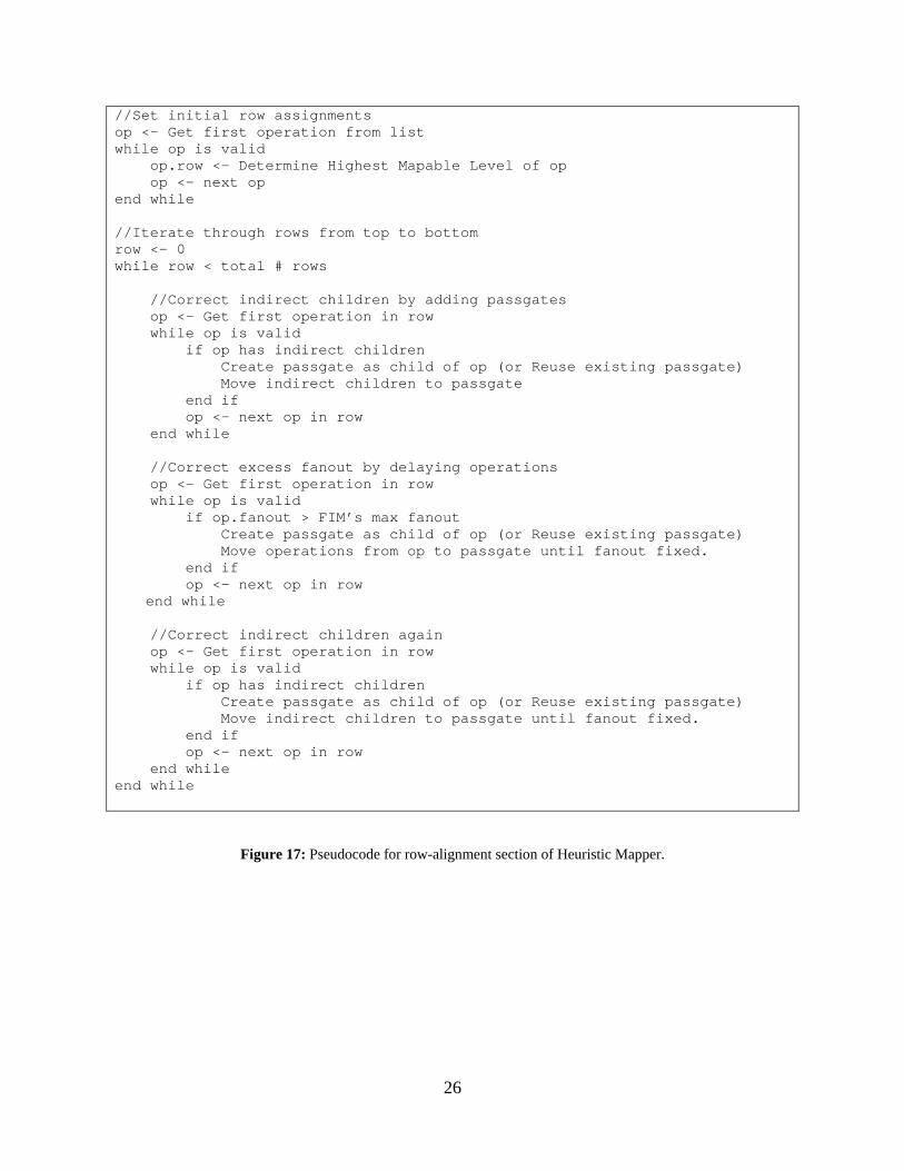
the mapper. Figure 17 shows pseudocode for the entire row-assignment portion of the Heuristic
Mapper. When iterating through the rows, the passgate correcting section is performed twice in
order to ensure that operations that were delayed in the fanout correction section are still
connected to all of their parents (the parents must be available in or passed to the row directly
above them).
26
//Set initial row assignments op <- Get first operation from list while op is valid op.row <- Determine Highest Mapable Level of op op <- next op end while //Iterate through rows from top to bottom row <- 0 while row < total # rows //Correct indirect children by adding passgates op <- Get first operation in row while op is valid if op has indirect children Create passgate as child of op (or Reuse existing passgate) Move indirect children to passgate end if op <- next op in row end while //Correct excess fanout by delaying operations op <- Get first operation in row while op is valid if op.fanout > FIM’s max fanout Create passgate as child of op (or Reuse existing passgate) Move operations from op to passgate until fanout fixed. end if op <- next op in row end while //Correct indirect children again op <- Get first operation in row while op is valid if op has indirect children Create passgate as child of op (or Reuse existing passgate) Move indirect children to passgate until fanout fixed. end if op <- next op in row end while end while
Figure 17: Pseudocode for row-alignment section of Heuristic Mapper.

27
3.3 COLUMN ASSIGNMENTS
Finally the operations are ready to be assigned to functional units available in the Fabric.
Beginning with the first row each operation in a row is placed into a valid location. In order to
perform column assignment, a number of factors are employed to determine the best location for
a given operation considering how this decision will impact the placement of other operations in
the current row as well as the children and grandchildren of the given operation. The initial three
factors used to build the mapper are the Parent Dependency, Child Dependency, and Functional
Unit Desirability factors. The Parent Dependency states that an operation must be mapped such
that each input (parent) connection can be routed using the fabric interconnect. Using the
locations of the (already placed) parents and the interconnect capabilities of the Fabric allows for
building of the Parent Dependency Window (PDW), which contains a list of all valid Functional
Unit locations that the operation could be placed in while meeting this dependency. Figure 18
shows an example of PDW construction. Each arrow shows a possible connection using the
Fabric’s interconnect. Given this interconnect a node with parents subtract in column 6 and
addition in column 8 can only be placed into ALUs 6 and 7. It should be noted that the parent
dependency window is the only requirement for assigning to a Functional Unit. The other factors
are used to improve the mapability of the other operations in the current row as well as
operations in later rows.
28
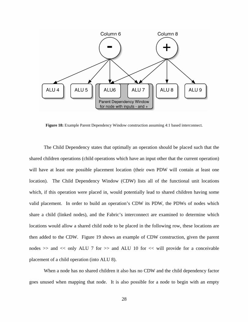
Figure 18: Example Parent Dependency Window construction assuming 4:1 based interconnect. The Child Dependency states that optimally an operation should be placed such that the
shared children operations (child operations which have an input other that the current operation)
will have at least one possible placement location (their own PDW will contain at least one
location). The Child Dependency Window (CDW) lists all of the functional unit locations
which, if this operation were placed in, would potentially lead to shared children having some
valid placement. In order to build an operation’s CDW its PDW, the PDWs of nodes which
share a child (linked nodes), and the Fabric’s interconnect are examined to determine which
locations would allow a shared child node to be placed in the following row, these locations are
then added to the CDW. Figure 19 shows an example of CDW construction, given the parent
nodes >> and << only ALU 7 for >> and ALU 10 for << will provide for a conceivable
placement of a child operation (into ALU 8).
When a node has no shared children it also has no CDW and the child dependency factor
goes unused when mapping that node. It is also possible for a node to begin with an empty

29
CDW (or a depleted CDW) if its PDW contains no locations that could satisfy the child
dependency.
Figure 19: Example of Child Dependency Window (CDW) construction.
The functional unit desirability (FUD) is often used as a tiebreaker during mapping when
locations are otherwise equal. FUD indicates the number of unplaced operations which contain
the given location in their PDW. In other words, how many operations “desire” to be placed into
the given location. Figure 20 shows the FUD construction using a few theoretical PDWs, ALU 0
is only found in the PDW of node >> which gives ALU0 a FUD value of 1. ALU 2 has the
highest FUD value at 3 as it is desired by the >>, mux, and << operations.

30
Figure 20: Example Functional Unit Desirability (FUD) construction.
3.3.1 Initial Heuristic Column Assignment
The initial heuristic relies only on the parent dependency, child dependency, and functional unit
desirability factors. Figure 21 shows the pseudocode for the initial heuristic column mapping of
a single row. Before mapping a row the child and parent dependency windows for each
operation are generated and the desirability of each functional unit is determined. Each
dependency window and desirability value is updated as functional units are filled by operation
placement. When a location is filled it is removed from the PDW and CDW of all operations
and the FUD values for all other locations in the mapped operation’s PDW are reduced
appropriately. In order to pick which operation to place, the remaining unmapped operations are
sorted such that the operation with the smallest PDW, smallest CDW, and least slack is at the
front of the list. The next operation list is resorted after each placement. This is partially
necessary such that the mapper will immediately deal with operations with a PDW of size zero or

31
a PDW of size one, both important (special) cases. In the PDW of size zero case, all the valid
locations the operation could be placed in have either been used or the parents of the operation
were mapped such that there would be no valid placement for the operation. In either case the
operation will be delayed until the next fabric row where the mapper will again try to place the
operation.

32
Create unsorted list of all operations in the given row op <- Get first operation from unsorted list while op is valid Generate PDW from location of parents/interconnect Add to desirability values op <- next op end while op <- Get first operation from unsorted list while op is valid Generate CDW from PDW and PDW of connected nodes op <- next op end while while unmapped ops > 0 Sort list of unmapped ops by PDW, CDW, slack op <- front of sorted list(smallest PDW, smallest CDW, least slack) Remove op from list of operations if PDW.size == 0 if Op is unary Exit Mapper, return UnMapable Code else Delay operation to next row if op.slack == 0 Increase high of problem graph Fix ALAP row for all unassigned nodes Search downstream of operation for passgates Absorb passgates Unassign everything in current row Restart Mapping current row end if else if PDW.size == 1 Place op in PDW's only location Update PDW,CDW,Desirability values. else //PDW.size > 1 if CDW.size == 1 Place op in CDW's only location Update PDW,CDW,Desirability values else if CDW.size > 1 Place op in CDW location with lowest desirability Update PDW,CDW,Desirability values else //no CDW, or CDW.size == 0 Place op in PDW location with lowest desirability Update PDW,CDW,Desirability values end if end while
Figure 21: Initial Heuristic column placement pseudocode.

33
Dynamically delaying an operation pushes it down to the next row and reconnects the
input edges using passgates (possibly new passgates). When pushing down an operation with
slack we know that there is a number of passgates that appear in later rows before the operation
is needed by the critical path. In order to correct the graph, after delaying an operation the
mapper will push the children of the given operation down (and then push their children, etc)
until encountering a passgate along each child-branch. The passgates (one along each branch of
children) are then absorbed and the graph is properly reconnected. If the operation has no slack
then no such passgates exist and an additional row will be added to the graph at the bottom
before the operation is delayed and passgates are absorbed. Figure 22 shows an example of
dynamically delaying an operation. The non-unary multiply operation is delayed to the next row,
two new pass operations are then added to fill the gap between the delayed node and its parents,
the subtract operation is then delayed to the next row and its pass operation child is absorbed
(removed).

34
Figure 22: Before/After Dynamically delaying an operation during mapping.
After delaying a node there may (and probably will) be new passgate operations that must
be mapped to the current row. In order to properly place them, the column assignment for the
current row restarts with all operations unassigned. However, in the case that the operation to
delay is a unary operation, then delaying would not fix the problem, instead the heuristic aborts
mapping. This is one of several issues that were remedied in later versions of the heuristic
(explained in the next sections).
Operations with only a single location in their PDW are placed in that location. When
the operation has more than one PDW location, the heuristic picks the location that has the
lowest desirability value and is also found in the CDW (assuming the CDW exists and has

35
nonzero size). Although the initial heuristic does well for several benchmarks, when using
highly connected Fabric Models, performance degrades quickly when the connectivity is reduced
and certain benchmarks become unsolvable.
3.3.2 Refining the Heuristic
In order to improve the results of the Heuristic Mapper a number of additional factors were
added to the heuristic. These changes were aimed at improving the placement of operations to
facilitate the eventual mapping of descendent operations. A priority node queue was added to
deal with the unmapable unary operations problem. To make the heuristic feasible for solutions
with less connectivity, an additional level of lookahead was implemented adding a Grandchild
dependency and associated grandchild dependency window (GDW). The following sections
examine each of these changes.
3.3.3 Optimizing Child Dependency: Potential Linked Placement Values
Although the initial algorithm uses the CDW to narrow the number of locations to consider, it
treats all locations in the CDW as equally good to use. In general that is not the case. While all
CDW locations theoretically allow each child operation to be placed, the ability to place them is
also tied to the placement of linked operations (“shared parents”). In order to increase the
likelihood that the child nodes will be mapped, the CDW concept is expanded to include a
Potential Linked Placement (PLP) value. The PLP value of each child dependency window
location is found by considering (for each child) the number of PDW locations of linked
operations that could be used while allowing the child operation(s) to be placed, assuming that
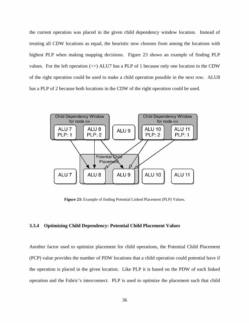
36
the current operation was placed in the given child dependency window location. Instead of
treating all CDW locations as equal, the heuristic now chooses from among the locations with
highest PLP when making mapping decisions. Figure 23 shows an example of finding PLP
values. For the left operation (>>) ALU7 has a PLP of 1 because only one location in the CDW
of the right operation could be used to make a child operation possible in the next row. ALU8
has a PLP of 2 because both locations in the CDW of the right operation could be used.
Figure 23: Example of finding Potential Linked Placement (PLP) Values.
3.3.4 Optimizing Child Dependency: Potential Child Placement Values
Another factor used to optimize placement for child operations, the Potential Child Placement
(PCP) value provides the number of PDW locations that a child operation could potential have if
the operation is placed in the given location. Like PLP it is based on the PDW of each linked
operation and the Fabric’s interconnect. PLP is used to optimize the placement such that child

37
operations can be mapped while PCP optimizes the placement to increase the mapping flexibility
of the child operation. Practically PCP is used to break ties where multiple locations have the
same PLP value.
3.3.5 Dealing with unary operations
In the initial heuristic, unary operations which run out of PDW locations before being placed will
cause the mapper to abort. Two changes were made to facilitate mapping unary operations.
First, when encountering a unary node with an empty PDW, the mapper attempts to “create” an
open spot that would allow the unary operation to be placed. The operations in each of the
locations in the unary node’s original PDW (before any operations in the current row were
mapped) are checked to see if any of them could move to an alternative position. If at least one
of them can, then the mapper reassigns a movable operation and places the unary operation in the
vacated spot. Otherwise the unary operation is placed into a priority node queue before
unassigning all operations in the current row and restarting column assignment. The column
assignment code was then modified so that priority nodes are mapped befefore non-priority
nodes. The priority queue can grow as additional hard to place unary operations are found.
However, if a priority node is found to be unmapable after given priority status the mapper is
forced to abort. Fortunately in practice this occurs rarely.
3.3.6 Picking Next Operation to Map
In the initial heuristic, choosing an operation to map relied primarily on the size of each
operation’s PDW. The revised version incorporates the priority node queue as well as resorting

38
the list to map highly connected nodes sooner. Priority nodes are placed before non-priority
nodes with the most recently prioritized nodes handled first. These nodes remain in the priority
queue until the current row is successfully mapped. This is done so that all the difficult unary
operations can be mapped if possible. After all priority nodes are placed, the nodes with PDW of
size 0 and 1 are handled in the original sort order (smallest PDW, smallest CDW, least slack
first). Following the special cases, the mapper resorts the list of unassigned operations. This
time the node with the smallest CDW (when considering only the CDW locations with maximum
PLP value), most linked nodes (nodes which share a child), most 2nd level linked nodes (share a
grandchild), and lowest slack is placed first in the list. Nodes without a CDW are placed at the
end of the list and, therefore, mapped last. This ordering optimizes the placement of the highly
connected nodes, which makes it easier to place their child operations in the next row.
3.3.7 Force System
The initial heuristic was unable to solve certain benchmarks within a reasonable fabric size due
to its inability to “converge” (i.e. bring to the point of making the shared children mapable)
problem nodes to map their shared children. In the case where two operations were far apart
from each other, they would also have empty CDWs. The mapper would place these nodes into
their PDW locations with lowest desirability. Often this would move the two operations further
apart instead of closer. Without a mechanism to ‘converge’ operations with shared children the
practical use of the heuristic was limited to small applications on highly connected fabrics. To
remedy this issue a system of forces is employed that assigns a force value to each location in the
PDW. The force system attempts to choose the location that can potentially satisfy the most
child operations, and it is optimized to prefer locations that provide linked nodes with as many

39
valid placements as possible. However, the system only performs its full logic when at least one
linked node can converge within the next two rows (2 row lookahead). If additional rows will be
required, then the system simply tries to move the linked nodes as close together as possible.
3.3.8 Grandchild Dependency
The initial heuristic was seriously limited by its effectively single row of lookahead. Operations
that needed to “converge” in two rows could be placed on opposite ends of the Fabric making it
impossible to pull the parent operations close enough to map a child operation without delaying
the child until a later row. To improve the overall quality of the mappings (reduce delays and
height), the second level of lookahead was added which gives the mapper one row to bring
operations that share a grandchild into positions that make the grandchild potentially mapable
(before having to delay operations). The grandchild dependency states that optimally an
operation should be placed such that the shared grandchildren operations could have at least one
possible placement location (their PDWs will contain at least one location). The Grandchild
Dependency Window is constructed in a similar manner as the CDW. Figure 24 shows an
example of GDW construction for two nodes with a shared child node. For the left node both
locations (4 and 5) could be used to reach a potential shared grandchild node, for the right node
only ALU10 and ALU11 could be used to reach the potential grandchild placement.
Nodes with no shared grandchildren simply have no GDW. Each location in a GDW also
has a Potential Linked Placement (PLP) value (similar to the CDW counterpart) that is used to
narrow the selection when the GDW holds multiple locations.

40
Figure 24: Example of Building the Grandchild Dependency Window (GDW).
3.3.9 Centering
One unintended result of using lowest functional unit desirability to determine placement is that
typically this pushes operations away from the center of the Fabric, which in general is the most
connected section and has functional units with high desirability values. Even after revising the
heuristic with many of the features already discussed the problem still existed as operations
(especially pass operations) with no CDW and GDW were forced to the outer edges of the
Fabric. The further out these operations were placed the longer it would take to converging them
with the nodes they shared children with. To alleviate this problem Distance From Center (DFC)
was added as a tiebreaker in several cases and a passgate centering procedure was executed after
each row had been completely mapped. Passgate centering moves non-linked passgate
operations into empty functional units closer to the fabric center which brings them closer to the
nodes which they will eventually need to converge with.

41
3.4 FINAL HEURISTIC
Figure 25 shows pseudocode for the final version which incorporates all of the described changes
into the heuristic. The method for using the heuristic on different Fabric Models is explained in
the next Section (4) with results examined in Section 6 and ideas for future improvements
presented in Section 7.
// Build PDW, CDW, Functional unit desirability\ Create unsorted list of all operations in the given row Generate PDW for each operation Determine functional unit desirability (FUD) values Generate CDW and PLP values for each operation Generate GDW and PLP values for each operation while unmapped ops > 0 if NOT (priority nodes all mapped) op <- next high priority node else Sort list of unmapped ops by PDW, CDW, slack op <- front of sorted list(smallest PDW, smallest CDW, least slack) Remove op from list of unmapped operations if PDW.size == 0 if Op is unary Attempt to create open spot if success Place into vacated spot else if op is a priority node Quit mapper else Make op high priority Restart Mapping current row end if end if else Delay operation to next row if op.slack == 0 Increase height of problem graph Fix ALAP row for all nodes Absorb passgates ‘downgraph’ Restart Mapping of current row end if else if PDW.size == 1 Place op in PDW's only location

42
else //PDW.size > 1 Resort operations list for highest connect node op <- front of list if CDW.size == 0 Choose location with force system else if CDW.size == 1 Choose only location in CDW else if CDW.size > 1 if GDW.size == 0 Choose location with highest PLP, highest PCP,
highest force value, lowest FUD else if GDW.size == 1 Choose only location in GDW else if GDW.size > 1
Choose location with highest GDW PLP value, highest PCP, lowest FUD, lowest DTC
else if No shared grandchildren Choose location with highest PLP, lowest FUD, highest PCP, lowest DTC
end if else if no shared children and no grandchildren Choose location with lowest desirability else if shared grandchildren if GDW.size == 0 Choose locations with force system else if GDW.size == 1 Choose only location in GDW else //GDW.size > 1
Choose location with highest GDW PLP, lowest FUD, lowest DTC
end if end if end if end while
Figure 25: Final Heuristic Column Assignments Pseudocode.

43
3.5 MAPPING REPRESENTATION
After the Heuristic Mapper has successfully mapped each row using the heuristic, the generated
mapping is recorded into a pair of files labeled the Order and Mapped Graph files. The Mapped
Graph holds the final form of the SDFG graph (including passgates) written in the DOT[13]
graph description language. The Order file lists the column assignment of each operation in the
graph. Together these files are used to represent a mapping that can be processed by the
software tools in the rest of the design flow.
3.6 MAPPING TO DEDICATED PASSGATES
During design space exploration, a set of Fabric Models that employ a mix of ALUs and
Dedicated Pass Units were tested to determine their performance (power/energy) characteristics
(Section 6.0). In order to perform mapping to a Fabric model with the dedicated passgates
feature, the column-assignment heuristic simply checks to see if a dedicated passgate is available
when mapping pass operations. Effectively this adds a dedicated passgate preference when
dealing with passgate operations. When generating the PDW for each non-pass operation, the
dedicated passgate locations are left out which prevents the heuristic from placing non-passgates
into dedicated passgate units. Although the current version can support these mixed ALU/DP
Fabric Models, further modifications will be needed to support more elaborate heterogeneous
models (Section 7).

44
4.0 FABRIC INTERCONNECT MODEL (FIM)
In order to facilitate creation of the design space exploration toolset a fabric model description
format was created. Built using extensible markup language (XML), the fabric interconnect
model (FIM) format specifies functional units used within the Fabric as well as the placement of
functional units and the interconnect between them. FIM allows for rapid writing and testing of
new fabric models and can be written directly by a user. In addition tools to support using the
FIM format were developed including verification, visualization and a programming interface.
4.1 EXTENSIBLE MARKUP LANGUAGE (XML)
Extensible Markup Language is an open-standard general-purpose markup language created by
the World Wide Web Consortium (W3C)[14]. XML provides a user and computer readable
format for holding data with the goal of utilization across multiple systems and applications.
Unlike languages such as HTML or VHDL, XML (syntax) tags do not come predefined. For the
most part the syntax (elements, attributes, and their properties ) of each XML file is specified by
the format designer. A major advantage to using XML is the large amount of support code
available allowing easy reading, writing, interpreting, and verification. Figure 26 shows an
example XML file which contains a short CD catalogue. CATALOGUE is the root element and

45
contains the type attribute as well as one or more <CD> elements. Each CD contains child
elements for TITLE, ARTIST, COUNTRY, PRICE, and YEAR.
<?xml version="1.0" encoding="utf-8"?> <CATALOGUE type="music"> <CD> <TITLE>But seriously</TITLE> <ARTIST>Phil Collins</ARTIST> <COUNTRY>USA</COUNTRY> <COMPANY>Atlantic / Wea</COMPANY> <PRICE currency="us">11.98</PRICE> <YEAR>1989</YEAR> </CD> </CATALOGUE>
Figure 26: A short CD catalogue written using XML.
4.2 FIM DEFINED
The FIM format was designed with the goal of creating a relatively simple method for the design
space exploration team to specify a fabric model. Each type of functional unit used in the Fabric
is defined using the FTU (Fabric Topological Unit) definition element <ftudefine>. All
operations a functional unit can perform are listed within an <ftudefine> using the operation
element <op>. In the proposed Fabric architecture, functional units are also required to have the
ability to perform a NoOp operation so that they can be turned off when not in use, the opcode
for this functionally is included as an attribute to <ftudefine>. The FIM specification can be
easily expanded to provide additional information about the fabric model.
One particular hardware feature which was added after the initial development is the
Integrated Constant (IC) feature (explained in detail in Section 6.0). The FIM specification was
expanded to add support for enabling/disabling of the Integrated Constants feature to functional

46
unit definition (<ftudefine>) elements using the attribute useic. The FIM code which specifies a
commonly used ALU is shown in Figure 27. This example indicates that the functional unit type
with name “alu0” can perform 18 operations in total; the opcode of each is defined using the
code attribute of each op element.
<ftudefine name="alu0" noop="10111" useic="false"> <op code="00001"> + </op> <op code="00010"> - </op> <op code="00011"> * </op> <op code="10011"> == </op> <op code="00111"> ^ </op> <op code="01110"> > </op> <op code="10000"> >= </op> <op code="01111"> < </op> <op code="10001"> <= </op> <op code="10010"> != </op> <op code="00100"> & </op> <op code="00101"> | </op> <op code="01001"> << </op> <op code="01011"> >> </op> <op code="00000"> pass </op> <op code="10100" order="reverse"> pass </op> <op code="11111"> mux </op> <op code="01000"> ! </op> </ftudefine>
Figure 27: FIM Code for an ALU Definition. The placement of functional units and interconnect is described using a series of tags
which create the pattern that represents a Fabric’s layout. Once defined the pattern can be used to
model a Fabric of any given height and width. The FIM Pattern description of an 8:1
multiplexer-based interconnect model is shown in Figure 28. The interconnect portion is
described using the <operand> and <range> tags. <range> describes the relative distances to the
left and right of the functional unit that could be reached for a particular operand. For example
<operand number=”0”> <range left = “-3” right = “4”/> </operand> gives operand zero access to

47
the outputs of the functional units in positions -3, -2, -1, +0, +1, +2, +3, and +4 relative to the
current functional unit’s position.
<rowpattern repeat="forever"> <row> <ftupattern repeat="forever"> <FTU type="alu0"> <operand number="0"> <range left ="-3" right ="4"/> </operand> <operand number="1"> <range left ="-3" right ="4"/> </operand> <operand number="2"> <range left ="-3" right ="4"/> </operand> </FTU> </ftupattern> </row> </rowpattern>
Figure 28: FIM Pattern Section for a standard 8:1 multiplexer based model. The elements (tags) and attributes that makeup the FIM file format are described in Table
1. The inclusion of the rowpattern and ftupattern elements allow for the creation of nearly any
conceivable configuration of functional units and interconnect. Consider Figure 29, in this
model odd numbered rows use 8:1 multiplexer-based interconnect while even numbered rows
use 4:1 multiplexer-based interconnect. In addition dedicated passgates (functional units that
only perform the pass operation) are used for the even half of the functional units and arithmetic
and logical units (ALUs) are used for the odd half. The FIM pattern code begins with a
rowpattern element with attribute repeat set to forever, this states that the rows described within
this rowpattern should be used to fill up the remaining rows of the Fabric Model(in this case all
of them). The first row element contains a single group of functional units which also is repeated
forever, meaning that the functional and topological (connectivity) definitions (FTUs) contained

48
within the pattern should be used to fill up all columns of the Fabric. The first FTU uses the alu0
functional unit, which is defined elsewhere in the same FIM file. All three operands are
connected to inputs -3, -2, -1, 0, +1, +2, +3, and +4 (8:1 multiplexer) via the operand and range
elements. The next FTU uses the pass type and only connects a single operand. Similarly the
second row element contains the ftupattern, FTU, operand, and range elements to describe an
alu0/pass pattern which connects each operand to inputs -1, 0, +1, and +2 (4:1 multiplexer).
Table 1: The Complete FIM specification: Elements and Attributes.
Element: Attributes: Description: FIM Root Element, can contain multiple ftudefine and rowpattern elements
ftudefine Defines a functional unit used in this fabric, can contain multiple op elements
name Name used to reference this definition noop Control Signal for NoOp operation (required)
useic Enable/Disable the Integrated Constant Hardware feature for this functional unit (disabled by default)
op Defines an operation the current functional unit can perform code Control Signal for this operation
reversed Designates the operation uses operand 1 as its first input and operand 0 as its second input (optional)
rowpattern A pattern made up of rows of functional units with interconnect. Contain 1 or more row elements
repeat Number of times the rowpattern should be repeated with "forever" designating unlimited repeating up to the height of the fabric.
row Represents a single row of a rowpattern, consists of 1 or more ftupatterns
ftupattern Defines a pattern of functional units in the current row
repeat Number of times the ftupattern should be repeated with "forever" designating unlimited repeating up to the width of the fabric
FTU Places a particular functional unit into an ftupattern; contains interconnect for one to three operand elements.
type The functional unit's type, should match the name attribute of one of the ftudefine elements
operand Defines interconnect of a particular operand of the current functional unit number Designates which operand is being described range Defines the relative range of locations reachable by the current operand left Range to the left right Range to the right

49
<rowpattern repeat="forever"> <row> <ftupattern repeat="forever"> <FTU type="alu0"><!-- 8:1 ALU --> <operand number="0"> <range left ="-3" right ="4"/> </operand> <operand number="1"> <range left ="-3" right ="4"/> </operand> <operand number="2"> <range left ="-3" right ="4"/> </operand> </FTU> <FTU type="pass"><!--8:1 Dedicated Pass--> <operand number="0"> <range left ="-3" right ="4"/> </operand> </FTU> </ftupattern> </row> <row> <ftupattern repeat="forever"> <FTU type="alu0"><!-- 4:1 ALU --> <operand number="0"> <range left ="-1" right ="2"/> </operand> <operand number="1"> <range left ="-1" right ="2"/> </operand> <operand number="2"> <range left ="-1" right ="2"/> </operand> </FTU><!-- 4:1 Dedicated Pass --> <FTU type="pass" commutative="true"> <operand number="0"> <range left ="-1" right ="2"/> </operand> </FTU> </ftupattern> </row> </rowpattern>
Figure 29: FIM Pattern Code for a 50% Dedicated Passgates, half 8:1 & half 4:1 interconnect.

50
4.3 SVG VISUALIZATION
In order to visualize fabric models software was developed to interpret a FIM file and produce a
Scalable Vector Graphics (SVG) representation. SVG is an XML-based method for defining
two-dimensional vector-based graphics [15]. Benefits of SVG include: optimized rendering for
all devices, support by a variety of applications (web browsers, image processors, etc), and
scaling to any size without loss of quality. Figure 30 shows a portion of a rendered SVG file for
the FIM file specified in Figure 29. Different colors are used to represent each column making it
possible to examine highly connected FIMs. Each functional unit lists its row / column location
within the Fabric, and below each input connection to a functional unit lists the operands which
have access to that particular input. For example R1C0 shows that operands 0, 1, and 2 have
access to R0C0, R0C1, and R0C2. For dedicated passgates (ex: R1C1) the inputs are all listed as
connecting to operand ‘P’ which is used to designate that the dedicated passgate is able to pass
any of the inputs through to the output.
Figure 30: Portion of a rendered SVG file for FIM shown in Figure 20.

51
4.4 FIM VERIFICATION
A number of methods exist which allow for the verification of XML files against a structural
definition. The most commonly used methods include Document Type Declarations
(DTDs)[16], RELAX NG[17], and XML Schema[18]. XML Schema provides an XML-based
method of describing the elements and attributes, the relationships between elements, and the
range of values allowed for content used for each element/attribute which fully describes what
could be written in an XML document. Figure 31 shows the XML Schema which describes the
format of the CD catalogue from Figure 26. Each XML element usable in the FIM is defined as
a complex or simple type which defines the type of data, attributes, and elements contained
within the element. The first defined element is CATALOGUE which contains only a sequence
of CD elements as well as having the required attribute type. The CD element type is defined as
a sequence containing the TITLE, ARTIST, COUNTRY, COMPANY, PRICE, and YEAR
elements. The first four can contain only string data, PRICE contains a currency value, and
YEAR uses the year datatype.

52
<?xml version="1.0" encoding="utf-8" ?> <xs:schema targetNamespace="http://cds.org/SimpleSchema.xsd" elementFormDefault="qualified" xmlns="http://cds.org/XMLSchema.xsd" xmlns:xs="http://www.w3.org/2001/XMLSchema"> <xs:element name="CATALOGUE"> <xs:complexType> <xs:sequence> <xs:element name="CD" maxOccurs="unbounded" type="CDType"/> </xs:sequence> <xs:attribute name="type" use="required" type="xs:string"/> </xs:complexType> </xs:element> <xs:complexType name="CDType"> <xs:sequence> <xs:element name="TITLE" type="xs:string"/> <xs:element name="ARTIST" type="xs:string"/> <xs:element name="COUNTRY" type="xs:string"/> <xs:element name="COMPANY" type="xs:string"/> <xs:element name="PRICE"> <xs:complexType> <xs:simpleContent> <xs:extension base="xs:decimal"> <xs:attribute name="currency" type="xs:string"/> </xs:extension> </xs:simpleContent> </xs:complexType> </xs:element> <xs:element name="YEAR" type="xs:gYear"/> </xs:sequence> </xs:complexType> </xs:schema>
Figure 31: XML Schema Definition (XSD) for Catalogue of CDs XML file shown in Figure 26. Numerous tools and XML engines support verifying XML files against an XML Schema
Definition (XSD). Software was created using Microsoft’s XML Core Services (MSXML)
Software development kit (SDK) [19] that verifies any XML file against any XML Schema
(XSD). The program was specifically used to provide verification of each FIM file created for
design space exploration against the FIM XSD. Additionally the FIM XSD can be used by XML
writing applications such as XMLSpy[20], XML Notepad[21], and Visual Studio[22] to shorten

53
the development time of FIM files by providing features such as code completion and visually
showing code which doesn’t meet the XSD specification.
4.5 FIM FRONT-END INTERFACE
A single FIM reader and FIM “front-end” object were developed to provide a single unified
interface that can be queried for information that any component of the Fabric CAD and design
space exploration tools may require. The FIM front-end takes as inputs the target fabric height
and width and a valid FIM file. The front-end then interprets the FIM’s pattern elements in order
to fill an internal fabric representation with functional units and interconnect. Relative range
values are interpreted and translated into absolute positions within the Fabric. The FIM front-
end object supports the ability to examine fan-ins, fan-outs, configuration signals, programmable
operations, and hardware features at any location in the Fabric. As new hardware features are
added they are first supported by the reader / front-end object, afterwards “back-end” tools such
as the Fabric Mapper can check for these features with simple query functions.

54
5.0 VERIFICATION AND CONFIGURATION
In order to test the results of a fabric mapper and generate the control signals needed for
configuring Fabric hardware, the FIM Fabric Printer tool was developed. The FIMFabricPrinter
analyzes a FIM to determine the length and number of all control signals needed for fabric
programming. The Printer then generates the set of control signals to configure the given fabric
in the form of Modelsim “do” files which allows for simulation and power analysis. To verify
that the mapping is valid each functional unit placement and use of interconnect is checked
against the capabilities of the FIM. In addition the Printer creates a visualization of the fabric
configured with the given mapping and generates statistics related to functional unit and
interconnect usage. When provided with input and results data, the tool can also generate a
verification file for use during hardware simulation to verify that the hardware is configured
properly and the simulation results are reliable.
5.1 PARAMETERS AND INPUTS
The Printer takes for input the Order and Mapped Graph files represent a mapping, a FIM format
file, and optionally an input/output data file. In addition a number of parameters are used to
customize the outputs (shown in Figure 32). The height and width of the target Fabric are
required by the FIM interpreter (FIM Front-End) to create a Fabric Model needed for the Printer.

55
Datasets and Verification Limit determine the number of input and output datasets which are
placed into .do files used for running simulations. Filltype and Output Mux Cardinality are used
to designate where and how the output values can be extracted from the Fabric. The output rows
are determined by the equation shown in Figure 33. Without this feature outputs must be passed
all the way to the last row of functional units in the Fabric. With the passgate Filltype, functional
units below the mapped operation that generates each result are programmed as passgates so that
the output results are available from the last row. The NoOp setting ignores the issue of
retrieving results completely and programs everything below the used portion of the Fabric as
NoOps.
Parameter Description Benchmark name Base name to use for all output file
Columns Width of target Fabric Rows Height of target Fabric
Datasets Number of input sets to place into result files
Verification limit Limits the number of input datasets used to the number of output datasets available
Fill type Output muxes, Passgates, or NoOps used to fill the bottom of the Fabric
Output mux cardinality Designates Cardinality to use for output mux feature (if enabled)
Figure 32: FIM Fabric Printer Parameters.
For i = 0 to k-1
⎡ ⎤)1/()1( +−− khih
k: Output multiplexer cardinality h: Fabric height
Figure 33: Equation to determine output rows when using outputmux fabric feature.

56
5.2 VERIFICATION AGAINST FIM
The FIMFabricPrinter reads the Order and Mapped Graph files and builds an internal mapping
representation using a matrix of operations and NoOps. Traversing the matrix, the Printer checks
each operation against the location’s functional unit to ensure it can be performed. The input
connection of each operand is then checked against the Fabric’s interconnect to ensure that a
connection between the two functional units is legitimate. Any error encountered during
verification will prevent the Printer from generating the configuration and output files. All
mapping errors are logged to aid in debugging incorrect mappings and mappers.
5.3 DYNAMICALLY DETERMINING MULTIPLEXER CONTROL SIGNALS
A key feature of the Fabric design space exploration flow is the ability to rapidly test a variety of
fabric models. Although the functional units used in a Fabric must be fully described in the FIM
model, including specifying the control signals to produce each operation the functional unit can
perform, the interconnect portion is described only by giving the range of inputs that it can
support. Determining the actual control signals for this interconnect has been automated by the
design flow to reduce the time to test alternative FIMs.
To determine the length of each multiplexer control signal, the number of inputs is
rounded up to the nearest standard multiplexer size (2:1, 4:1, 8:1, etc). Next each connection
(relative values given by <range> FIM elements) is assigned a binary value control signal
beginning with the leftmost connection receiving the greatest value and moving rightward.
Values range from (in decimal) 12 −n down to 0, n being the number of bits needed to control

57
the multiplexer. Figure 34 shows an example of input select control signal generation for a 4:1
mutliplexer. Relative range value -2 is assigned to the highest available binary value ‘11’, then
proceeding to the right each relative range value is assigned to the next highest binary value.
<range left ="-2" right ="1"/>
Figure 34: Example of control signal generation using 4:1 multiplexer.
5.4 BUILDING CONFIGURATION FILES
The Printer writes the control signals for each functional unit and interconnect multiplexer to a
series of ModelSim script files used for simulation. Each fabric row is controlled using a pair of
do files; one each for functional units and interconnect. The Printer begins at the first row of the
mapping matrix and processes each operation and NoOp from left to right. For each position the
operation control signal is retrieved from the parameterized fabric model and placed into the
corresponding row’s do file. Afterward multiplexer control signals are found for each operand by
performing a look up into the dynamically generated control signals. The first row will also

58
contain the number of input datasets used (as per the parameter) written in the form of force
commands which set the inputs to the functional units (with integrated constants). In addition a
verification (.vf) file is generated if results data is available. The file can be compared against
simulation results to verify that the fabric configuration and simulation model are correct.
5.5 GENERATING STATISTICS
While traversing the mapping matrix the Printer records functional unit and interconnect usage
statistics. For each row the Printer tracks the number of non-pass operations, passgate
operations, and NoOps. In addition it determines and records the minimum multiplexer needed
to implement each connection between operations (each usage of interconnect). These statistics
have proven helpful in the design space exploration process and provide guidance on which
alternative FIMs to pursue.
5.6 GENERATING VISUALIZATION
FIMFabricPrinter produces a Scalable Vector Graphics (SVG) file which provides a
visualization of the parameterized Fabric configured with the given mapping. As shown in
Figure 35 the SVG displays the mapped function of each position in the Fabric as well as the
input and output nodes of the mapped SDFG. The utilized interconnect is shown as lines between
functional units. Unused functional units are set to NoOps and are displayed as grey boxes.

59
Figure 35 : SVG representation of Sobel mapping on 8:1-based FIM.

60
6.0 PERFORMANCE RESULTS
In this section we will employ five metrics of performance: Mapping Height, Mapper Runtime,
Power, Energy, and Delay. In order to judge the performance of the Heuristic Mapper we
compare the mappings produced by the heuristic against those produced by two alternative
methods, a Mixed Integer Linear Program Mapper and a Constraint Program Mapper, using all
five metrics. These comparisons were performed using the 8:1, 5:1, 4:1, and 3553:1 fabric
interconnect models. In order to understand the progression of the Heuristic Mapper we will also
compare the mapping sizes of the Initial, Advanced, and Final versions using the 5:1 FIM. The
results of running the Heuristic Mapper on a variety of FIMs are also included. Finally the 8:1
results will be compared against FPGA and ASIC implementations to determine how the Fabric
compares against these hardware alternatives.
To perform power/energy comparisons the appropriate fabric configuration files were
generated for each combination of Mapper and FIM. For each combination the minimum size
(width/height) needed to implement all seven benchmarks was used to create an Application
Specific Fabric (ASF)1. Each ASF was implemented in parameterized VHDL and synthesized
using 160nm OKI standard cell ASIC process. Synthesis was executed using Design Compiler
1Team member Gayatri Mehta handled creation, simulation, & power/energy profiling of the hardware
fabric models.

61
and power was estimated using PrimePower; both tools from Synopsys [23]. PrimePower is
considered to provide power estimations within approximately 10% accuracy of a Spice
simulation of the circuit [24].
6.1 FABRIC INTERCONNECT MODELS
6.1.1 8:1-based Fabric Models
The 8:1-based Fabric Models employ 8:1 multiplexers to build each stripe of interconnect
between rows of Functional Units. Therefore each operation has a maximum fan-in of eight and
a maximum fanout of eight. The 8:1-based Fabric Models employed by this thesis pull from
inputs in the column positions -3, -2, -1, +0, +1, +2, +3, and +4 relative to the position of any
given Functional Unit. A portion of the rendered SVG representation of this type of Fabric
Model is shown in Figure 36. Notice that each operand of each functional unit can connect to
any of the eight inputs.
Figure 36: Visualization of 8:1-based Interconnect.

62
6.1.2 4:1-based Fabric Models
The 4:1-based Fabric Models employ 4:1 multiplexers to build each stripe of interconnect.
Figure 37 shows a portion of the rendered SVG representation of this Model. Each operation has
a maximum fan-in of four and a maximum fan-out of four. Each of the multiplexers used for the
ALU operands pulls from locations -1, +0, +1, and +2 relative to the position of any given
Fucntional Unit.
Figure 37: SVG Visualization of 4:1-based Interconnect. The 5:1 Fabric Interconnect Model also builds stripes of interconnect using a 4:1
multiplexers. Figure 38 shows a portion of the rendered SVG representation of this model.
Notice that the first operand (labeled 0) pulls from relative locations -2, -1, +0, and +1 while the
other operands (1 and 2) are unchanged from the 4:1 Models. Through this one minor change a
maximum fan-in and fan-out of five can be achieved with only a minor change in hardware (the
additional wiring to connect the extra input). As shall be seen, the increased connectivity allows
the Heuristic Mapper to generate considerable improved mappings.
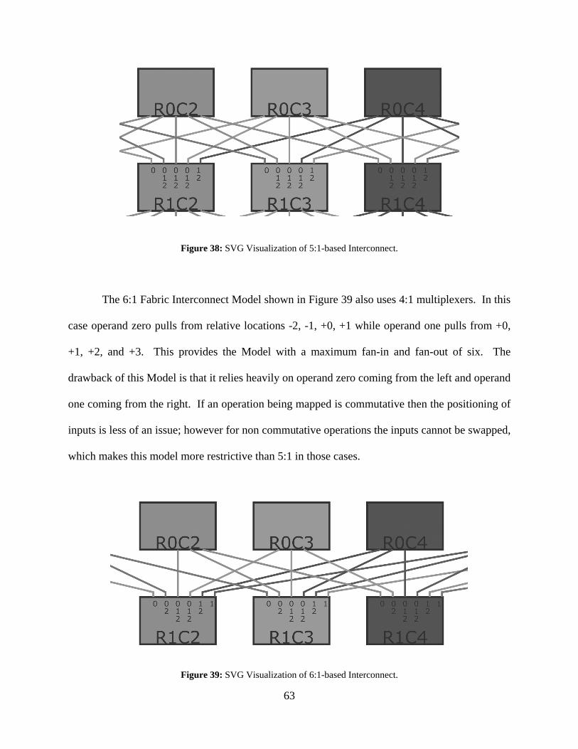
63
Figure 38: SVG Visualization of 5:1-based Interconnect. The 6:1 Fabric Interconnect Model shown in Figure 39 also uses 4:1 multiplexers. In this
case operand zero pulls from relative locations -2, -1, +0, +1 while operand one pulls from +0,
+1, +2, and +3. This provides the Model with a maximum fan-in and fan-out of six. The
drawback of this Model is that it relies heavily on operand zero coming from the left and operand
one coming from the right. If an operation being mapped is commutative then the positioning of
inputs is less of an issue; however for non commutative operations the inputs cannot be swapped,
which makes this model more restrictive than 5:1 in those cases.
Figure 39: SVG Visualization of 6:1-based Interconnect.

64
6.1.3 3553:1-based Fabric Models
The 3553 Fabric Models employ a mixture of 2:1 and 4:1 multiplexers. Figure 39 shows a
portion of the rendered SVG representation of this model. Every first and fourth Functional Unit
in the Fabric is connected to its operands using three 2:1-multiplexers, they are configured such
that operand 0 connects to relative locations -1 and +0, while operands 1 and 2 are connected to
operands +0 and +1. This gives these locations a maximum fan-in and fan-out of 3. Every
second and third location uses the 5:1 configuration already described.
Figure 40: SVG Visualization of 3553:1-based Interconnect.
6.2 BENCHMARK KERNELS
For the current stage of Fabric development, a set of seven benchmark kernels from image and
signal processing algorithms was employed for testing of the Fabric design flow. All of these
benchmarks except Laplace and Sobel are part of the Mediabench suite [25]. Laplace and Sobel
were created using commonly available source code.

65
Adpcm Encoder and Decoder: An Adaptive Differential Pulse Code Modulation,
ADPCM is employed in audio and video compression algorithms including video
conferencing and Voice over IP [26].
GSM: The core channel encoding kernel used in wireless communications for digital
mobile phones. GSM-based services are used by more than 2 billion people across the
world making it the most popular cell phone standard [27].
Idct Column and Row: Column-wise and row-wise decompositions of a two-dimensional
inverse discrete cosine transformation (DCT) that was extracted from the MPEG II
decoder. MPEG II is the video compression algorithm commonly used to decode DVD
video[28].
Laplace: An algorithm to find the edges between features in an image. The Laplace edge
detection technique calculates these edges by computing the 2nd derivative in two
directions of 5 x 5 blocks of pixels.
Sobel: Another edge detection algorithm. The Sobel edge detection technique calculates
these edges by computing the gradient in two directions of 3 x 3 blocks of pixels.
As we can see from Table 2, idctcol and idctrow are the largest benchmarks in terms of
actual operations; in addition they also have the highest density values. Density here meaning:
(total number of operations + passgates) / height. All benchmarks become “thinner” and less
dense when Integrated Constants(IC) are used in the Fabric. In general we find that less dense
benchmarks are easier to map meaning that the Heuristic Mapper is more likely to find a near
optimal solution.

66
Table 2: Benchmark sizes
ASAP Regular Constants(RC)
ASAP Integrated Constants(IC) ASAP
#operations #passgates Width Density #passgates Width Density Heightadpcm_decoder 29 79 16 8.31 48 11 5.92 13 adpcm_encoder 36 130 17 10.38 77 12 7.06 16 GSM 28 129 14 8.72 63 9 5.06 18 idctcol 61 88 20 12.42 44 11 8.75 12 idctrow 52 57 17 10.9 34 11 8.6 10 Laplace 29 17 15 5.75 4 13 4.13 8 Sobel 24 18 10 4.67 7 8 3.44 9
6.3 SOLUTION IMPROVEMENT DURING DEVELOPMENT OF HEURISTIC
The motivation behind heuristic improvement was primarily the desire to find decent mappings
for 5:1 and other limited interconnect FIMs. Table 3 shows the differences between three distinct
versions of the heuristic. Table 4 shows the results of running the heuristic with each version.
Using 5:1 FIM the initial mapper was only able to solve 5 out of 7 benchmarks; this was
remedied by the Force system mechanic added into the revised version. In order to further
improve the results a second level of lookahead was added into the final version. Additionally
time to map is significantly reduced in post-initial versions, although it should be noted that no
version was optimized for runtime.

67
Table 3: Heuristic Mapper Versions Summary.
Initial Version: Basic Rule (PDW)
One level of lookahead (CDW).
ALU Desirability: Used for tiebreaking. Revised Version: Optimized for future child placement (Potential Connectivity).
“Force” system to converge problematic operations so that they
could be solved.
Row & Passgate Centering Final Version: Two levels of lookahead added to all logic (GDW, Forces).
Priority Operations
Support for some heterogeneous fabrics (Dedicated Passgates)
Table 4: Heuristic Versions: Processing time & added rows for 5:1-based Standard FIM.
Initial Revised Final
Time to Map (s) Added rows
Time to Map (s) Added rows
Time to Map (s) Added rows
Adpcm_decoder 9 11 3 0 4 0 Adpcm_encoder 79 13 16 2 10 2 GSM 18 3 1 1 3 1 Idctcol 37 no solution 11 12 8 6 Idctrow 15 no solution 4 6 6 3 Laplace < 1 0 < 1 0 1 0 Sobel 1 1 < 1 1 1 0

68
6.4 COMPARING MAPPING TECHNIQUES
Currently there exist two alternative methods of solving the Fabric Mapping problem, the first
being a Mixed Integer Linear Program (MILP) 2. In the MILP solution a set of object functions
and constraints are used to define the mapping problem. A MILP solver then searches for a
solution which correctly minimizes the objective value while meeting all the constraints. In our
case the objective function is to minimize the number of edges (fabric interconnect links) that are
infeasible with the given FIM. In order to find a valid mapping, the MILP solver must find a
solution with objective value equal to zero, so that there are no “infeasible” connections. The
constraints ensure that only each operation occupies one position, operations are placed in the
correct row, and that each position is used by only one operation.
Unlike the Heuristic Mapper this solution will only find an “optimal’ result, meaning a
result where all operations are mapped into the row they are found in a row-aligned SDFG. The
MILP solution lacks the ability to “push” operations down to later rows. ILOG’s CPLEX 9.0
was employed to execute the MILP solver [29].
The second alternative method employs Constraint Programming and a heuristic
approach to create a valid mapping3. In Constraint Programming a set of relations between
variables are described using constraints. In addition a distribution strategy is included to
determine how the search space is explored. Much like the MILP Solution, constraints are used
2 The MILP Mapper was developed by team member Mustafa Baz.
3 The Constraint Programming Mapper was developed by Fabric team member Professor Brady Hunsaker
of the Industrial Engineering Department.

69
to define the mapping problem. The Constraint Program was implemented in the open-source
Mozart/Oz environment [30].
Similarly to MILP the CP is unable to dynamically “push” operations down to later rows,
however by adding additional automation we are able to add additional rows of pass operations
to the CP’s row-aligned input, these additional rows add a degree of flexibility allowing
additional benchmarks to be solved.
6.4.1 Runtime Comparison
Table 5 lists runtime numbers found by running each mapper on a Pentium IV 3.0 GHz machine.
Dashes indicate that no valid mapping could be found. MILP consumes significantly more time
compared to the CP and heuristic solutions. In general runtime increases as the connectivity
decreases.
Table 5: CPU Runtime (seconds) of each mapper for 3553:1, 4:1, 5:1 & 8:1 standard FIMs.
3553:1 Standard
FIM 4:1 Standard FIM 5:1 Standard FIM 8:1 Standard FIM MILP CP H MILP CP H MILP CP H MILP CP H Adpcm_decoder 539 1 7 539 1 7 960 2 4 155 1 < 1 Adpcm_encoder - - 64 - 86 16 2746 277 10 306 1 4 GSM - 25 48 2613 1 4 1801 2 3 514 1 < 1 Idctcol - - 25 - 307 19 7587 7 8 894 10 1 Idctrow - 512 8 - 512 8 2049 36 6 460 1 < 1 Laplace 181 23 2 181 23 2 46 47 1 13 27 < 1 Sobel - - 1 104 < 1 1 33 1 1 37 < 1 < 1

70
6.4.2 Mapping Size Comparison
In Table 6 we see that the 8:1 mapping is a relatively easy problem for each mapper, while the
5:1 model requires the heuristic and CP to add up to 6 rows. At 4:1 the MILP is no longer able
to solve all the benchmarks, and at 3553 the CP begins to fail as well.
Table 6: Rows added by each mapper for 3553:1, 4:1, 5:1 & 8:1 standard FIMs.
3553:1 Standard
FIM 4:1 Standard FIM 5:1 Standard FIM 8:1 Standard FIM MILP CP H MILP CP H MILP CP H MILP CP H Adpcm_decoder 0 0 8 0 0 2 0 0 0 0 0 0 Adpcm_encoder - - 14 - 3 4 0 7 2 0 0 0 GSM - 0 4 0 0 3 0 0 1 0 0 0 Idctcol - - 16 - 4 15 0 0 6 0 0 0 Idctrow - 12 9 - 3 8 0 1 3 0 0 0 Laplace 0 1 1 0 2 0 0 1 0 0 1 0 Sobel - - 1 0 0 0 0 0 0 0 0 0
6.4.3 Power / Energy Comparisons
Table 7 and 8 show the power and energy usage of each FIM / Mapper combination where all
seven benchmarks are mapable. Looking at the 8:1 results shown in Figure 41, each mapper
produced similar energy numbers ( <10% variance ) with the heuristic performing slightly better
overall.

71
Table 7: Power (mW) of fabric mappings for 3553:1, 4:1, 5:1, & 8:1 standard FIMs across methods.
3553:1 Std FIM
4:1 Std FIM 5:1 Std FIM 8:1 Std FIM
H CP H MILP CP H MILP CP H Adpcm_decoder 3.4 2.9 2.7 2.9 2.7 2.7 3.52 3.38 3.5 Adpcm_encoder 20.2 18.5 15.4 17.4 17.7 18.0 20.68 19.84 20.08 GSM 16.2 19.6 17.6 19.6 19.4 19.3 22.19 22.27 21.45 Idctcol 35.3 31.9 38.9 28.9 27.2 33.4 31.87 31.95 29.09 Idctrow 40.1 40.7 47.2 31.8 31.2 39.4 25.74 36.57 36.22 Laplace 3.0 4.8 3.1 4.0 4.4 3.9 4.42 5.03 4.3 Sobel 3.5 5.0 3.5 5.0 5.0 4.7 5.68 5.81 5.65
Table 8: Energy (pJ) of fabric mapping for 3553:1, 4:1, 5:1, & 8:1 standard FIMs across methods.
3553:1 Std
FIM 4:1 Std FIM 5:1 Std FIM 8:1 Std FIM H CP H MILP CP H MILP CP H Adpcm_decoder 175 113 137 107 100 105 151 145 151 Adpcm_encoder 1068 738 785 662 672 722 910 873 884 GSM 937 880 986 843 832 868 1110 1114 1073 Idctcol 2259 1624 2412 1415 1334 1704 1753 1757 1600 Idctrow 2445 1955 2785 1464 1436 1889 1858 1902 1883 Laplace 146 172 147 137 150 139 172 196 168 Sobel 183 193 175 188 185 181 244 250 243
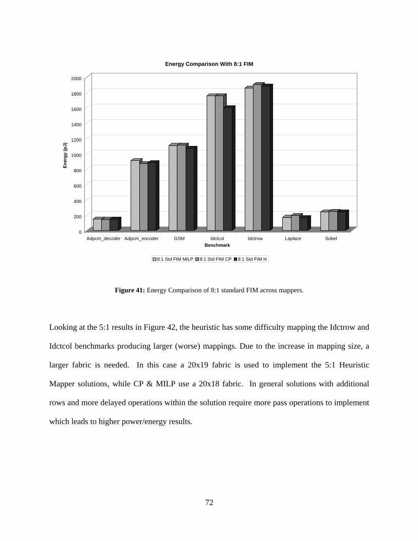
72
0
200
400
600
800
1000
1200
1400
1600
1800
2000
Ener
gy (p
J)
Adpcm_decoder Adpcm_encoder GSM Idctcol Idctrow Laplace SobelBenchmark
Energy Comparison With 8:1 FIM
8:1 Std FIM MILP 8:1 Std FIM CP 8:1 Std FIM H
Figure 41: Energy Comparison of 8:1 standard FIM across mappers. Looking at the 5:1 results in Figure 42, the heuristic has some difficulty mapping the Idctrow and
Idctcol benchmarks producing larger (worse) mappings. Due to the increase in mapping size, a
larger fabric is needed. In this case a 20x19 fabric is used to implement the 5:1 Heuristic
Mapper solutions, while CP & MILP use a 20x18 fabric. In general solutions with additional
rows and more delayed operations within the solution require more pass operations to implement
which leads to higher power/energy results.

73
0
200
400
600
800
1000
1200
1400
1600
1800
2000
Ener
gy (p
J)
Adpcm_decoder Adpcm_encoder GSM Idctcol Idctrow Laplace SobelBenchmarks
Energy Comparison WIth 5:1 FIM
5:1 Std FIM MILP 5:1 Std FIM CP 5:1 Std FIM H
Figure 42: Energy Comparison of 5:1 standard FIM across mappers.
6.4.4 Delay Comparison
Table 9 shows the time to execute (delay) of each mapping when implemented on the Fabric.
Figure 43 shows the average delay for each mapper/FIM combination. For 8:1 the delay of all
mappings is almost identical. For 5:1 & 4:1 the heuristic solutions perform slightly worse. Only
the heuristic is able to solve all the benchmarks for 3553:1, however these mappings are
particularly large and thus produce longer delays.
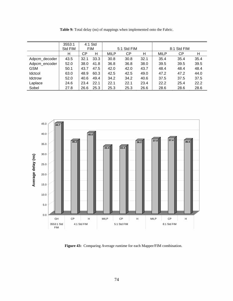
74
Table 9: Total delay (ns) of mappings when implemented onto the Fabric.
3553:1 Std FIM
4:1 Std FIM 5:1 Std FIM 8:1 Std FIM
H CP H MILP CP H MILP CP H Adpcm_decoder 43.5 32.1 33.3 30.8 30.8 32.1 35.4 35.4 35.4 Adpcm_encoder 52.0 38.0 41.8 36.8 36.8 38.0 39.5 39.5 39.5 GSM 50.1 43.7 47.5 42.0 42.0 43.7 48.4 48.4 48.4 Idctcol 63.0 48.9 60.3 42.5 42.5 49.0 47.2 47.2 44.0 Idctrow 52.0 40.6 49.4 34.2 34.2 40.6 37.5 37.5 37.5 Laplace 24.6 23.4 22.1 22.1 22.1 23.4 22.2 25.4 22.2 Sobel 27.8 26.6 25.3 25.3 25.3 26.6 28.6 28.6 28.6
44.7
36.2
40.0
33.4 33.4
36.2 37.0 37.4 36.5
0.0
5.0
10.0
15.0
20.0
25.0
30.0
35.0
40.0
45.0
Ave
rage
del
ay (n
s)
GH CP H MILP CP H MILP CP H
3553:1 StdFIM
4:1 Std FIM 5:1 Std FIM 8:1 Std FIM
Figure 43: Comparing Average runtime for each Mapper/FIM combination.

75
6.4.5 Analysis
From the mapping results we can see that both 4:1 and 3553:1 FIMs are significantly harder to
map for, while 8:1 and 5:1 are relatively easier for the mappers to handle. Due to the nature of
each mapper, MILP and CP tend to find closer to optimal (no rows added) solutions, while the
heuristic is willing to delay operations into lower rows. This property also allows the heuristic to
solve even the tough 3553:1 and 4:1 cases. However, at that point, the quality of the solutions
becomes so poor that the use of these FIMs becomes questionable.
Comparing the mappers using 8:1 we can see that while each mapping’s power / energy
results are relatively similar, the MILP takes 13X to 894X as much processing (mapping) time as
the Heuristic Mapper. Clearly there is an implicit tradeoff made for each of these mappers. The
Heuristic Mapper is designed to find any valid mapping, while MILP and CP spend significant
time exploring possible solutions in order to come up with an optimal solution. In addition we
can see that additional improvements to the heuristic will be required if the 4:1 and 3553:1 FIMs
are going to be used over the 5:1 and 8:1 solutions.
6.5 HEURISTIC MAPPER RESULTS ON A VARIETY OF FABRIC MODELS
After finding the poor performance of all mappers on “less connected” FIMs (those using smaller
multiplexer sizes) the Heuristic Mapper was used to explore mapping on alternative FIM models
described in Table 10.

76
Table 10: FIM variations, each could be coupled with any level of interconnect (8:1, 5:1, etc).
Standard (std): Identical ALUs for all positions.
All inputs must be passed down from the top of the Fabric.
Integrated Constants (IC):
Identical ALUs for all positions.
Constant inputs preloaded instead of passing down.
Dedicated Passgates (DP):
Dedicated passgates used for some portion of fabric (50%, 33%, etc)
All inputs must be passed down from the top of the fabric.
The goal of Integrated Constants (IC) is to reduce the complexity of the mapping
problems by loading certain constant inputs (inputs which remain constant across all iterations of
a particular benchmark) into latches located inside each ALU.
The goal of Dedicated Passgates (DP) is to reduce the area/power/energy of the Fabric by
replacing some percentage of ALUs in each row with dedicated passgate units (DPU). In
addition to being much smaller, these dedicated passgates use less power and energy than
standard ALUs.
6.5.1 Integrated Constants Results
Table 11 shows the number of rows that were added for the heuristic to find a solution for each
benchmark using the 8:1, 5:1 and 3553:1 FIMs with and without Integrated Constants. By
removing constant inputs from the SDFG, the problem size is significantly reduced (see Table 2),
resulting in smaller solutions. The energy results shown in Figure 44 present a mixed picture.
There is a power and energy cost to pay for the additional hardware required to handle constant

77
preloading. In smaller benchmarks (decoder, laplace, sobel), the additional hardware is not worth
the cost because these problems are already comparatively easy to map. In the larger benchmarks
(idctrow, idctcol, gsm), the benefits significantly outweigh the costs. The decision to use
Integrated Constants (IC) or Regular Constants (RC) should be determined by considering the
size of all the benchmarks a user wanted the Fabric to perform.
Table 11: Rows added to solve 8:1, 5:1, and 3553:1 Std & IC FIMs using Heuristic Mapper.
8:1 Std 8:1 IC 5:1 Std 5:1 IC 3553:1 Std 3553:1 IC Adpcm_decoder 0 0 0 1 8 4 Adpcm_encoder 0 0 2 1 14 5 GSM 0 0 1 0 4 0 Idctcol 0 0 6 0 16 4 Idctrow 0 0 3 4 9 8 Laplace 0 0 0 0 1 1 Sobel 0 0 0 0 1 2
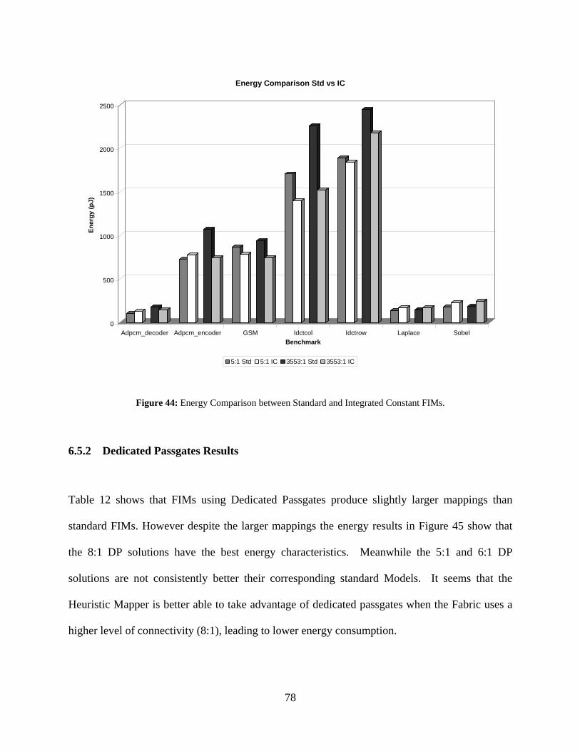
78
0
500
1000
1500
2000
2500
Ener
gy (p
J)
Adpcm_decoder Adpcm_encoder GSM Idctcol Idctrow Laplace SobelBenchmark
Energy Comparison Std vs IC
5:1 Std 5:1 IC 3553:1 Std 3553:1 IC
Figure 44: Energy Comparison between Standard and Integrated Constant FIMs.
6.5.2 Dedicated Passgates Results
Table 12 shows that FIMs using Dedicated Passgates produce slightly larger mappings than
standard FIMs. However despite the larger mappings the energy results in Figure 45 show that
the 8:1 DP solutions have the best energy characteristics. Meanwhile the 5:1 and 6:1 DP
solutions are not consistently better their corresponding standard Models. It seems that the
Heuristic Mapper is better able to take advantage of dedicated passgates when the Fabric uses a
higher level of connectivity (8:1), leading to lower energy consumption.

79
Table 12: Rows added to solve 8:1, 6:1, and 5:1 Standard & Dedicated Passgate FIMs
8:1 6:1 5:1
Std 50% DP
33% DP Std 50% DP 33% DP Std
50% DP
33% DP
Adpcm_decoder 0 0 0 1 1 0 0 1 1 Adpcm_encoder 0 1 0 2 4 2 2 2 2 GSM 0 0 0 0 0 1 1 1 0 Idctcol 0 2 1 5 6 6 6 7 6 Idctrow 0 1 0 3 4 5 3 4 4 Laplace 0 2 1 1 2 1 0 3 1 Sobel 0 0 0 0 1 0 0 2 0
0
200
400
600
800
1000
1200
1400
1600
1800
2000
Ener
gy (p
J)
Adpcm_decoder Adpcm_encoder GSM Idctcol Idctrow Laplace Sobel
Energy Comparison Standard VS Dedicated Passgates
8:1 Std 8:1, 50% DP 8:1, 33% DP6:1 Std 6:1, 50% DP 6:1 33% DP5:1 Std 5:1, 50% DP 5:1, 33% DP
Figure 45: Energy Comparison between 8:1, 5:1, Standard and Dedicated Passgates FIMs.

80
6.6 COMPARING FABRIC VS CURRENT HARDWARE TECHNOLOGIES
Now we will consider how well the Fabric meets the stated goal of providing an FPGA
replacement while providing ASIC like power/energy results. Figure 46 shows a comparison
between custom ASIC implementations of the benchmarks, fabric implementations using the 8:1
50% DP FIM, FPGA implementations using a Xilinx Virtex 2P, and running each benchmark in
software on an Intel XScale 733 MHz processor. Table 13 shows the power results for each
implementation, while Table 14 provides the energy results. To determine the FPGA results,
delay was computed using post place-and-route simulations in ModelSim and these were used to
estimate power using Xilinx Xpower. XScale processor results were found using the XTREM
[31] SimpleScalar ARM simulator.
While the ASIC implementation receives the best energy scores, overall in terms of
power and energy performs the Fabric far outclasses the FPGA and XScale implementations.
Power improvements over the Virtex-2P ranged from 68X to 369X and energy improvements
from 38X to 127X. Compared to the XScale the Fabric used 7X to 92X less power and 87X to
1199X less energy.
The Fabric comes close to matching the power characteristics of a custom
implementation, at worst the Fabric uses 3X the power and 13X as much energy as
corresponding ASIC implementations. The power and energy difference between the Fabric and
direct ASIC implementations are primary due to the configurable interconnect found in the
Fabric implementation, which is significantly more complex than the dedicated routing used in
each custom ASIC implementation. Another portion of the difference comes from the increased
power and delay inherent in using configurable functional units over single purpose units.

81
Table 13: Power (mW) usage of benchmark implementations on ASIC, Fabric, FPGA, and XScale.
ASIC
(0.16um) Fabric (8:1, 50% DP)
(0.16 um) Virtex-2P (0.13um)
XScale 733 MHz (0.18um)
Adpcm_decoder 0.802 2.28 842.01 195.84 Adpcm_encoder 4.99 14.6 1085.19 194.81 GSM 6.97 15.4 1049.01 198.68 Idctcol 16.13 24.6 4277.55 218.36 Idctrow 16.47 30.7 4258.87 215.82 Laplace 4.21 4.6 903.38 382.12 Sobel 5.088 4.11 1122.5 378.19
Table 14: Energy (pJ) usage of benchmark implementations on ASIC, Fabric, FPGA, and XScale.
ASIC
(0.16um) Fabric (8:1, 50% DP) (0.16
um) Virtex-2P (0.13um)
XScale 733 MHz (0.18um)
Adpcm_decoder 7.218 98 10946 117557 Adpcm_encoder 79.84 642 24959 152020 GSM 139.4 770 34617 67763 Idctcol 354.86 1353 136882 336626 Idctrow 329.4 1596 127766 139562 Laplace 42.1 156 13551 177017 Sobel 61.056 177 22450 109800

82
1
10
100
1000
10000
100000
1000000
Ener
gy (p
J)
Adpcm_decoder Adpcm_encoder GSM Idctcol Idctrow Laplace SobelBenchmark
Energy Comparison Between Hardware Technologies
ASIC (0.16um) Fabric (8:1, 50% DP) (0.16 um)Virtex-2P (0.13um) Xscale (0.18um)
Figure 46: Energy Comparison between hardware technologies
6.7 COMPARING HEURISTIC AGAINST AS SOON AS POSSIBLE
During the course of developing the Fabric design flow, the ability to generate an As Soon As
Possible mapping of an SDFG was added to the design flow path. The ASAP mappings can
potentially be used as actual fabric mappings for a high connectivity homogeneous fabric. The
power / energy results of running these ASAP mappings can be used as a baseline to compare
new FIMs. Table 15 shows an energy comparison between a 32:1-based FIM used to implement
the ASAP mappings and the most (power / energy) efficient mappings the Heuristic Mapper

83
could generate (8:1, 50% dedicated passgates). By employing the Heuristic Mapper the energy
usage can be reduced by a significant amount (32% to 64%) from the simplistic ASAP approach.
Table 15: Energy (pJ) comparison ASAP Schedule Solutions VS. Heuristic Mapper Solutions.
32:1 using
ASAP 8:1, 50% DP using Heuristic Mapper
Times improvement % reduction
Adpcm_decoder 274 98 2.79 64.22% Adpcm_encoder 1535.04 642 2.39 58.15% GSM 1533.3 770 1.99 49.78% Idctcol 2712.5 1353 2.00 50.12% Idctrow 4045.8 1596 2.53 60.54% Laplace 232.76 156 1.49 32.81% Sobel 325.115 177 1.84 45.64%

84
7.0 CONCLUSION
The electronic design automation suite presented by this thesis provides a complete C to Fabric
design flow for the Coarse-Grain Reconfigurable Fabric target platform. This suite allows for
rapid design space exploration of the Fabric device during Research and Development while also
providing the basis for a full CAD toolset to be used with the device. Each of the contributions
of this thesis assist in accomplishing these overarching goals.
Heuristic Mapper: Handles the central problem of configuring the Fabric to perform a given
functionality. Very fast, expandable, and capable of solving the mapping problem for a
wide range of Fabric Models.
Fabric Interconnect Model (FIM): Facilitates rapid testing of Fabric Models by providing
the mechanism for configuring the Heuristic and overall Fabric EDA suite to target a
specific Fabric Models. Eliminates the need to reprogram Heuristic for every Fabric Model.
FimFabricPrinter: Provides quality assurance of the Fabric Mappings at an early stage
through visualization and verification of Fabric Mappings. Integrates support for simulation
and power/performance analysis of Fabric hardware through generation of set of Modelsim
script (“.do”) files facilitating the simulation of the Fabric device configured with any given
Mapping.

85
The results of comparing Fabric implementations against FPGA, ASIC, and embedded
processor demonstrates that the Reconfigurable Coarse-grain Fabric can function as a viable
FPGA or ASIC alternative for system and system-on-a-chip designers interested in a low power
reconfigurable solution for accelerating application kernels. Even with a perfect Mapper and
fully optimized Fabric it will not be possible to match the power, energy, and performance
characteristics of a full custom ASIC implementation. This is partly due to the overhead of using
multiplexer based connectivity in the Fabric as opposed to the direct routing found in ASIC
implementations. The usage of reconfigurable ALUs also increases the size of the device
leading to increased wire length and increased power and reduced performance. These factors
cannot be eliminated but they can be minimized through careful design space exploration of the
Fabric and development of capable Mapping techniques to efficiently configure the Fabric.
7.1 FUTURE DIRECTIONS
While the Heuristic Mapper performs admirably for 8:1-based Fabric Models, its capabilities
seem to scale poorly as the amount of connectivity decreases. This is made obvious by the poor
performance of particular 5:1 and 3553:1 based models. A number of approaches could be
considered to remedy this issue, however it is the author’s opinion that the most promising
modifications lie in the area of incorporation elements of Global Lookahead. In addition further
modifications should be considered in order to better target heterogeneous Fabric Models using
the heuristic.

86
7.1.1 Global Lookahead Information
While the Heuristic Mapper performs well for the group of medium sized benchmarks analyzed
in the results section, and typically does well for Fabric Models with high connectivity (such as
8:1-based models), when the connectivity is reduced (5:1, 355:1, etc) or benchmark sizes
increases significantly, the quality of the mapping generated degrades. Particularly the Heuristic
Mapper shows problems when mapping SDFGs where a number of inputs are passed down
though several fabric rows before being used with another operation. The passed value may be a
non-constant input or a value which is calculated early in the Fabric but then unused for several
rows. In these cases the passgates which carry the value will be pushed away from the center of
the Fabric, typically this will move the operation away from the operations that it eventually
shares children with. As the fabric width increases or the connectivity decreases, the two rows of
lookahead prove to be insufficient because the number of columns which need to be crossed to
put the nodes into position requires the child operations to be delayed.
Fixing this problem will require the heuristic to integrate global lookahead information.
Instead of looking at the nodes that share children in the next two rows, the heuristic should
consider all convergences in the next several rows or potentially the entire graph. Depending on
the amount of connectivity (8:1, 4:1, etc), the heuristic can determine when to begin pushing
linked nodes together such that their shared children will be mapable without repeated delays.
7.1.2 Global Lookahead Heuristic For First Row Mapping
To complete the transformation to a global lookahead heuristic, the first row of the Fabric should
be placed using a lookahead specialized heuristic. The goal of the first row heuristic should be to

87
map the top row such that the distance between each operation is dependent on the row in which
the operations share a child operation. Operations which share a child in the next few rows
should be mapped close together to avoid delays, while operations that share a child in a later
row can be mapped near enough for the modified heuristic to bring them together soon enough
such that their child operations are mapable with a minimal amount of delay. This improvement
would eliminate the common problem where nodes that converge three rows from the top are
mapped on opposite ends of the Fabric. This heuristic will be in effect planning out every
convergence in the graph. By adding global lookahead elements, the heuristic can expect to
reduce the number of dynamic delays, the number of passgates needed, and the height of the
mapping. By reducing the size of the mapping these changes should lead to further power and
energy improvement over the current mappings.
7.1.3 Handling Heterogeneous Fabric Models
The Heuristic Mapper was designed upon the basic idea that in a homogenous fabric only the
distance between nodes prevents their child operations from being mapable. Therefore, when a
child node is found to be unmapable, the heuristic will simply delay the node and try to push the
introduced passgates as close together as possible such that eventually the child node will be
mapable. In heterogeneous fabric models there exists the additional problem of having no
functional unit within range that can execute the child operation. The changes that would be
required to optimize mapping to heterogeneous fabrics are more difficult to generalize.
However, there are a few modifications which would benefit the heuristic when mapping to any
heterogeneous fabric.

88
The first modification would alter the parent dependency window building procedure
such that locations which cannot perform an operation are not added into the window. This
functionality is already partly implemented to support dedicated passgates. Another change
would modify the behavior in all cases where the child operation is unmapable. Although the
parents should still be pushed closer together they also need to be pushed in the direction of a
location in some later row that can perform the child operations. The CDW and GDW
generation logic could also be modified to incorporate information on each functional unit’s
capabilities when considering the potential locations for child operations. These changes should
improve the quality of mapping when using fabric models with multiple types of functional
units.

89
APPENDIX A
FABRIC INTERCONNECT MODEL FILES
A.1 FIM FOR 8:1-BASED, 50% DEDICATED PASSGATES FABRIC
<?xml version="1.0" encoding="utf-8"?> <!--This XML file defines a 8 to 1 Interconnect pattern --> <FIM xmlns="http://composers.ee.pitt.edu/FIM.xsd" xmlns:xsi="http://www.w3.org/2001/XMLSchema-instance" xsi:schemaLocation="http://composers.ee.pitt.edu/FIM.xsd FIM.xsd"> <!-- This is for the standard alu we've been working with--> <ftudefine name="alu0" noop="10111" useic="false"> <op code="00001"> + </op> <!-- non-comm subtract --> <op code="00010"> - </op> <op code="00011"> * </op> <op code="10011"> == </op> <op code="00111"> ^ </op> <op code="01110"> > </op> <op code="10000"> >= </op> <op code="01111"> < </op> <op code="10001"> <= </op> <op code="10010"> != </op> <op code="00100"> & </op> <op code="00101"> | </op> <op code="01001"> << </op> <op code="01011"> >> </op> <op code="00000"> pass </op> <op code="10100" order="reverse"> pass </op> <op code="11111"> mux </op> <op code="01000"> ! </op> </ftudefine>

90
<!-- 8:1 passgate --> <ftudefine name="pass" noop="0" useic="false"> <op code="1" order="std">pass</op> </ftudefine> <rowpattern repeat="forever"> <row> <ftupattern repeat="forever"> <!-- 8:1 ALU --> <FTU type="alu0"> <operand number="0"> <range left ="-3" right ="4"/> </operand> <operand number="1"> <range left ="-3" right ="4"/> </operand> <operand number="2"> <range left ="-3" right ="4"/> </operand> </FTU> <!-- 8:1 Dedicated Pass --> <FTU type="pass"> <operand number="0"> <range left ="-3" right ="4"/> </operand> </FTU> </ftupattern> </row> </rowpattern> </FIM>

91
A.2 FIM ROWPATTERN FOR 8:1-BASED, 33% DEDICATED PASSGATES FABRIC
<rowpattern repeat="forever"> <row> <ftupattern repeat="forever"> <!-- 8:1 ALU --> <FTU type="alu0"> <operand number="0"> <range left ="-3" right ="4"/> </operand> <operand number="1"> <range left ="-3" right ="4"/> </operand> <operand number="2"> <range left ="-3" right ="4"/> </operand> </FTU> <!-- 8:1 ALU --> <FTU type="alu0"> <operand number="0"> <range left ="-3" right ="4"/> </operand> <operand number="1"> <range left ="-3" right ="4"/> </operand> <operand number="2"> <range left ="-3" right ="4"/> </operand> </FTU> <!-- 8:1 Dedicated Pass --> <FTU type="pass"> <operand number="0"> <range left ="-3" right ="4"/> </operand> </FTU> </ftupattern> </row> </rowpattern>

92
A.3 FIM ROWPATTERN FOR 8:1-BASED STANDARD FABRIC
<rowpattern repeat="forever"> <row> <ftupattern repeat="forever"> <FTU type="alu0"> <operand number="0"> <range left ="-3" right ="4"/> </operand> <operand number="1"> <range left ="-3" right ="4"/> </operand> <operand number="2"> <range left ="-3" right ="4"/> </operand> </FTU> </ftupattern> </row>
</rowpattern>

93
A.4 FIM ROWPATTERN FOR 5:1-BASED 50% DEDICATED PASSGATES FABRIC
<rowpattern repeat="forever"> <row> <ftupattern repeat="forever"> <FTU type="alu0"> <operand number="0"> <range left ="-2" right ="1"/> </operand> <operand number="1"> <range left ="-1" right ="2"/> </operand> <operand number="2"> <range left ="-1" right ="2"/> </operand> </FTU> <!-- 8:1 Pass, made from 2 4:1 inputs --> <FTU type="pass" commutative="true"> <operand number="0"> <range left ="-3" right ="0"/> </operand> <operand number="1"> <range left ="1" right ="4"/> </operand> </FTU> </ftupattern> </row> </rowpattern>

94
A.5 FIM ROWPATTERN FOR 5:1-BASED 33% DEDICATED PASSGATES
<rowpattern repeat="forever"> <row> <ftupattern repeat="forever"> <FTU type="alu0"> <operand number="0"> <range left ="-2" right ="1"/> </operand> <operand number="1"> <range left ="-1" right ="2"/> </operand> <operand number="2"> <range left ="-1" right ="2"/> </operand> </FTU> <FTU type="alu0"> <operand number="0"> <range left ="-2" right ="1"/> </operand> <operand number="1"> <range left ="-1" right ="2"/> </operand> <operand number="2"> <range left ="-1" right ="2"/> </operand> </FTU> <!-- 8:1 Pass, made from 2 4:1 inputs --> <FTU type="pass" commutative="true"> <operand number="0"> <range left ="-3" right ="0"/> </operand> <operand number="1"> <range left ="1" right ="4"/> </operand> </FTU> </ftupattern> </row> </rowpattern>
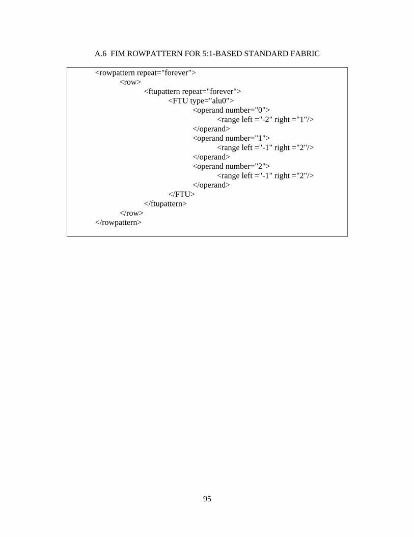
95
A.6 FIM ROWPATTERN FOR 5:1-BASED STANDARD FABRIC
<rowpattern repeat="forever"> <row> <ftupattern repeat="forever"> <FTU type="alu0"> <operand number="0"> <range left ="-2" right ="1"/> </operand> <operand number="1"> <range left ="-1" right ="2"/> </operand> <operand number="2"> <range left ="-1" right ="2"/> </operand> </FTU> </ftupattern> </row> </rowpattern>

96
A.7 FIM ROWPATTERN FOR 4:1-BASED STANDARD FABRIC
<rowpattern repeat="forever"> <row> <ftupattern repeat="forever"> <FTU type="alu0"> <operand number="0"> <range left ="-1" right ="2"/> </operand> <operand number="1"> <range left ="-1" right ="2"/> </operand> <operand number="2"> <range left ="-1" right ="2"/> </operand> </FTU> </ftupattern> </row> </rowpattern>

97
A.8 FIM ROWPATTERN FOR 3553:1-BASED STANDARD FABRIC
<rowpattern repeat="forever"> <row> <ftupattern repeat="forever"> <!-- 3:1 --> <FTU type="alu0"> <operand number="0"> <range left ="-1" right ="0"/> </operand> <operand number="1"> <range left ="0" right ="1"/> </operand> <operand number="2"> <range left ="0" right ="1"/> </operand> </FTU> <!-- A 5:1 --> <FTU type ="alu0"> <operand number="0"> <range left ="-2" right ="1"/> </operand> <operand number="1"> <range left ="-1" right ="2"/> </operand> <operand number="2"> <range left ="-1" right ="2"/> </operand> </FTU> <!-- A 5:1 --> <FTU type ="alu0"> <operand number="0"> <range left ="-2" right ="1"/> </operand> <operand number="1"> <range left ="-1" right ="2"/> </operand> <operand number="2"> <range left ="-1" right ="2"/> </operand> </FTU> <!-- 3:1 --> <FTU type="alu0"> <operand number="0"> <range left ="-1" right ="0"/> </operand>

98
<operand number="1"> <range left ="0" right ="1"/> </operand> <operand number="2"> <range left ="0" right ="1"/> </operand> </FTU> </ftupattern> </row>
</rowpattern>

99
APPENDIX B
XML SCHEMA FOR FABRIC INTERCONNECT MODEL
<?xml version="1.0" encoding="utf-8" ?> <xs:schema targetNamespace="http://composers.ee.pitt.edu/FIM.xsd" elementFormDefault="qualified" xmlns="http://composers.ee.pitt.edu/FIM.xsd" xmlns:xs="http://www.w3.org/2001/XMLSchema"> <!-- FIM is the root node, it consists of 1 or more rowpattern elements--> <xs:element name="FIM"> <xs:complexType> <xs:sequence> <xs:element name="ftudefine" maxOccurs="unbounded" type="FTUDefineType"/> <xs:element name="rowpattern" maxOccurs="unbounded" type="RowPatternType"/> </xs:sequence> </xs:complexType> </xs:element> <!-- The FTUDefineType consists of 1 or more Op elements and requires a name attribute--> <xs:complexType name="FTUDefineType"> <xs:sequence> <xs:element name="op" type="OpType" maxOccurs="unbounded"/> </xs:sequence> <xs:attribute name="name" use="required"/> <xs:attribute name="noop" use="required"/> <xs:attribute name="useic" use="optional" default="true"> <xs:simpleType> <xs:restriction base="xs:string"> <xs:enumeration value="false"/> <xs:enumeration value="true"/>

100
</xs:restriction> </xs:simpleType> </xs:attribute> </xs:complexType> <!-- The OpType consists provides an op and the corresponding opcode optionally it can designate if this is a "reversed" op using the order attribute--> <xs:complexType name="OpType" mixed="true"> <xs:attribute name="code" use="required"/> <xs:attribute name="order" use="optional" default="std"> <xs:simpleType> <xs:restriction base="xs:string"> <xs:enumeration value="std"/> <xs:enumeration value="reverse"/> </xs:restriction> </xs:simpleType> </xs:attribute> </xs:complexType> <!-- The RowPatternType consists of 1 or more row elements , and can have the repeat attribute--> <xs:complexType name="RowPatternType" > <xs:sequence> <xs:element name="row" type="RowType" maxOccurs="unbounded"/> </xs:sequence> <xs:attribute name="repeat" type="xs:string" default="1" use="optional"/> </xs:complexType> <!-- A RowType repesents a single row, consists of 1 or more ftupattern elements--> <xs:complexType name="RowType" > <xs:sequence> <xs:element name="ftupattern" maxOccurs="unbounded" type="FTUPatternType"/> </xs:sequence> </xs:complexType> <!-- FTUPatternType consists of 1 or more FTUs, has the optional attribute repeat--> <xs:complexType name="FTUPatternType" > <xs:sequence> <xs:element name="FTU" maxOccurs="unbounded" type="FTUType"/> </xs:sequence> <xs:attribute name="repeat" default="1" type="xs:string" use="optional"/> </xs:complexType>

101
<!-- FTUType consists of 1 to 3 operands , has required type field, has optional commutative attribute FTU means Fabric Topological Unit --> <xs:complexType name="FTUType"> <xs:sequence> <xs:element name="operand" maxOccurs="3" type="OperandType"/> </xs:sequence> <xs:attribute name="commutative" type="xs:boolean" use="optional" default="false"/> <xs:attribute name="type" type="xs:string" use="required"/> </xs:complexType> <!-- OperandType consists of 1 or more range elements, and the required attribute "number"--> <xs:complexType name="OperandType"> <xs:sequence> <xs:element name="range" maxOccurs="unbounded" type="RangeType"/> </xs:sequence> <xs:attribute name="number" type="xs:unsignedInt" use="required"/> </xs:complexType> <!-- RangeType consists of only the attributes: left, and right, which give the "ranges"--> <xs:complexType name="RangeType"> <xs:attribute name="left" type="xs:int"/> <xs:attribute name="right" type="xs:int"/> </xs:complexType> </xs:schema>

102
BIBLIOGRAPHY
[1] A. K. Jones, R. Hoare, D. Kusic, J. Fazekas, and J. Foster, An FPGA-based VLIW Processor
with Custom Hardware Execution, in Proc. of the ACM International Symposium on Field-Programmable Gate Arrays (FPGA) 2005, pp. 107-117.
[2] A. K. Jones, R. Hoare, D. Kusic, J. Fazekas, G. Mehta, and J. Foster, A VLIW Processor with Hardware Functions: Increasing Performance While Reducing Power, IEEE Transactions on Circuits and Systems II, Vol. 53, No. 11, November 2006, pp. 1250-1254.
[3] E. Mirsky and A. Dehon, “Matrix: A reconfigurable computing architecture with configurable instruction distribution and deployable resources,” in Proceedings of the IEEE Workshop on FPGAs for Custom Computing Machines, April 1996.
[4] J. R. Hauser and J. Wawrzynek, “Garp: A MIPS processor with a reconfigurable coprocessor,” in IEEE Symposium on FPGAs for Custom Computing Machines, K. L. Pocek and J. Arnold, Eds. Los Alamitos, CA: IEEE Computer Society Press, 1997, pp. 12–21. [Online]. Available: citeseer.nj.nec.com/hauser97garp.html
[5] S. Hauck, T. W. Fry, M. M. Hosler, and J. P. Kao, “The chimaera reconfigurable functional unit,” in IEEE Symposium on FPGAs for Custom Computing Machines(FCCM), 1997, pp. 87–96.
[6] C. Ebeling, D. C. Cronquist, and P. Franklin, “Rapid - reconfigurable pipelined datapath,” in the 6th International Workshop on Field-Programmable Logic and Applications, 1996.
[7] C. E. et al., “Mapping applications to the rapid configurable architecture,” in Proc. of the IEEE Symposium on FPGAs for Custom Computing Machines, 1997.
[8] B. Levine and H. Schmit, “Piperench: Power & performance evaluation of a programmable pipelined datapath,” presented at Hot Chips 14, Palo Alto, CA, August 2002.
[9] H. Schmit, D. Whelihan, A. Tsai, M. Moe, B. Levine, and R. R. Taylor, “Piperench: A virtualized programmable datapath in 0.18 micron technolog,” in Proceedings of the IEEE Custom Integrated Circuits Conference, 2002.
[10] Elixent, “The reconfigurable algorithm processor,” http://www.elixent.com/
103
[11] PACT-XPP, “Xpp-lib core overview,” http://www.pactcorp.com/
[12]MathStar, “Field programmable object array architecture”, http://www.mathstar.com/literature.html.
[13] DOT Language http://en.wikipedia.org/wiki/DOT_language
[14] World Wide Web Consortium. http://www.w3.org/XML/
[15] Scalable Vector Graphics Working Group. http://www.w3.org/Graphics/SVG/
[16] Document Type Definition. http://en.wikipedia.org/wiki/Document_Type_Definition
[17] RELAX NG http://relaxng.org/
[18] W3C XML Schema http://www.w3.org/XML/Schema
[19] XML Developer Center. http://msdn2.microsoft.com/en-us/xml/default.aspx
[20] XMLSpy - XML editor for modeling, editing, transforming, & debugging XML technologies http://www.altova.com/
[21] XML Notepad 2007 http://msdn2.microsoft.com/en-us/xml/default.aspx
[22] Microsoft Visual Studio – http://msdn.microsoft.com/vstudio
[23] Synopsys Inc., “Design compiler and primepower manual,” http://www.synopsys.com
[24] R. Georing, “Synopsys launches power tool,” EETimes, May 2000.
[25] Lee, C., Potkonjak, M., Magione-Smith, W. K., 1997. Mediabench: A tool for evaluating and synthesizing multimedia and communications systems. Proceedings of the International Symposium on Microarchitecture.
[26] Adaptive Differential Pulse Code Modulation http://www.everything2.com/index.pl?node_id=1377999
[27] Global System for Mobile Communications. http://en.wikipedia.org/wiki/Global_System_for_Mobile_Communications
[28] MPEG-2. http://en.wikipedia.org/wiki/Mpeg_2
[29] ILOG CPLEX. http://www.ilog.com/products/cplex/

104
[30] Roy, P. V. (Ed.), 2005. Multiparadigm Programming inMozart/Oz, Second International
Conference, MOZ 2004, Charleroi, Belgium, October 7-8, 2004, Revised Selected and Invited Papers. Vol. 3389 of Lecture Notes in Computer Science. Springer.
[31] C. Gilberto, M. Martonosi, J. Peng, R. Ju, and G. Lueh, “XTREM: A power simulator for the Intel XScale core,” in Proc. ACM LCTES, 2004.