Embed Size (px)
Citation preview
ELECTRON TRANSPORT AT THE NANOSCALE
Lecture Notes, preliminary version
Geert Brocks
December 2005

ii

Chapter 1
Electron transport in one dimension
This chapter gives a simple introduction to scattering problems in one dimension and theirrelation to the conductance of one-dimensional systems at the level of introductory quantummechanics. Purely one-dimensional systems are of limited practical use, but their simplicityallows one to introduce the basic physics using simple mathematics only. Sec. 1.1 recapitulatesthe concept of a quantum current, as defined in introductory quantum mechanics. The Landauerformula expresses the electronic conductance or resistance of a system as a scattering problem.1
A naive derivation is given in Sec. 1.2.2 Sec. 1.3 introduces some elementary folklore ofscattering theory, the transfer matrix and the scattering matrix, using the ubiquitous squarebarrier potential as an example. Techniques to solve scattering problems for any one-dimensionalpotential are introduced in Sec. 1.4. These will be generalized to three-dimensional problems inthe next chapter. In particular I focus on so-called “mode matching”, which is the most accessibletechnique. I discuss its relation to the “Green function” and the “embedding” techniques,two other currently used methods. The techniques are illustrated by a simple model, whichconsists of a straightforward discretization of the one-dimensional Hamiltonian.3 This model ismathematically equivalent to a simple tight-binding model of a quantum wire of atoms, as isshown in Sec. 1.5.4
1.1 Quantum currents
1.1.1 Probability currents
The probability current J(x, t)
J(x, t) =ih
2m
µΨ∂Ψ
∂x
∗−Ψ∗∂Ψ
∂x
¶(1.1)
is defined such that
dPab(t)
dt= J(a, t)− J(b, t) (1.2)
1It is also called the Landauer-Buttiker formalism. The first idea to relate the conductance of a small systemto its scattering matrix comes from Landauer. Buttiker made a generalization to multi-terminal devices, whichhave more than two electrodes.
2Secs. 1.1 and 1.2 are adaptations from my lecture notes for the introductory bachelor course in quantummechanics.
3The model is didactical and not designed to be the most efficient way to solve this scattering problem. Themath is easy, however, and the general ideas can be applied to more complicated systems.
4Secs. 1.3-1.5 consist of elements of lecture notes I am writing for a master course.
1
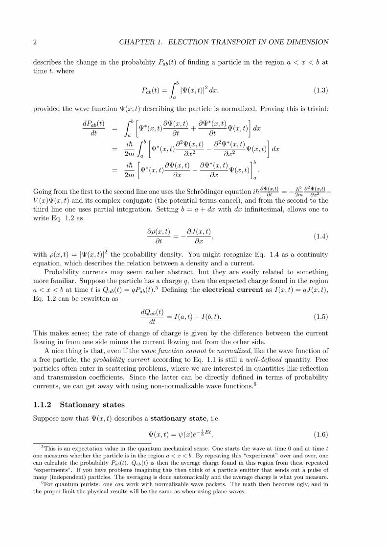
2 CHAPTER 1. ELECTRON TRANSPORT IN ONE DIMENSION
describes the change in the probability Pab(t) of finding a particle in the region a < x < b attime t, where
Pab(t) =
Z b
a|Ψ(x, t)|2 dx, (1.3)
provided the wave function Ψ(x, t) describing the particle is normalized. Proving this is trivial:
dPab(t)
dt=
Z b
a
·Ψ∗(x, t)
∂Ψ(x, t)
∂t+
∂Ψ∗(x, t)∂t
Ψ(x, t)
¸dx
=ih
2m
Z b
a
·Ψ∗(x, t)
∂2Ψ(x, t)
∂x2− ∂2Ψ∗(x, t)
∂x2Ψ(x, t)
¸dx
=ih
2m
·Ψ∗(x, t)
∂Ψ(x, t)
∂x− ∂Ψ∗(x, t)
∂xΨ(x, t)
¸ba
.
Going from the first to the second line one uses the Schrodinger equation ih∂Ψ(x,t)∂t = − h2
2m∂2Ψ(x,t)
∂x2+
V (x)Ψ(x, t) and its complex conjugate (the potential terms cancel), and from the second to thethird line one uses partial integration. Setting b = a + dx with dx infinitesimal, allows one towrite Eq. 1.2 as
∂ρ(x, t)
∂t= −∂J(x, t)
∂x, (1.4)
with ρ(x, t) = |Ψ(x, t)|2 the probability density. You might recognize Eq. 1.4 as a continuityequation, which describes the relation between a density and a current.
Probability currents may seem rather abstract, but they are easily related to somethingmore familiar. Suppose the particle has a charge q, then the expected charge found in the regiona < x < b at time t is Qab(t) = qPab(t).
5 Defining the electrical current as I(x, t) = qJ(x, t),Eq. 1.2 can be rewritten as
dQab(t)
dt= I(a, t)− I(b, t). (1.5)
This makes sense; the rate of change of charge is given by the difference between the currentflowing in from one side minus the current flowing out from the other side.
A nice thing is that, even if the wave function cannot be normalized, like the wave function ofa free particle, the probability current according to Eq. 1.1 is still a well-defined quantity. Freeparticles often enter in scattering problems, where we are interested in quantities like reflectionand transmission coefficients. Since the latter can be directly defined in terms of probabilitycurrents, we can get away with using non-normalizable wave functions.6
1.1.2 Stationary states
Suppose now that Ψ(x, t) describes a stationary state, i.e.
Ψ(x, t) = ψ(x)e−ihEt. (1.6)
5This is an expectation value in the quantum mechanical sense. One starts the wave at time 0 and at time tone measures whether the particle is in the region a < x < b. By repeating this “experiment” over and over, onecan calculate the probability Pab(t). Qab(t) is then the average charge found in this region from these repeated“experiments”. If you have problems imagining this then think of a particle emitter that sends out a pulse ofmany (independent) particles. The averaging is done automatically and the average charge is what you measure.
6For quantum purists: one can work with normalizable wave packets. The math then becomes ugly, and inthe proper limit the physical results will be the same as when using plane waves.
1.1. QUANTUM CURRENTS 3
Then one finds from Eq. 1.3
dPab(t)
dt= 0
and from Eqs. 1.2 and 1.1
J(x, t) = J = constant. (1.7)
The probability current is constant, i.e. independent of position and time.For example, consider a free particle with the wave function
ψ(x) = A eikx. (1.8)
From Eq. 1.3 we calculate
Pab = |A|2 (b− a). (1.9)
Since Pab is the probability of finding the particle in the interval between x = a and x = b, i.e.an interval of length b− a, we can interpret |A|2 as the probability density per unit length. Itis also called the particle density7
ρ = |A|2 . (1.10)
The probability current is easily calculated from its definition, Eq. 1.1
J =hk
m|A|2 = hk
mρ. (1.11)
According to de Broglie’s relation p = hk is the momentum of the particle and
v =hk
m=p
m(1.12)
is then the velocity of the particle. The electrical current is given by
I = qJ = qvρ, (1.13)
which is the usual definition of an electrical current, namely charge×velocity×density. For thewave function of Eq. 1.8 both velocity and density are constant, so the wave function describesa uniform current. Suppose q > 0; then if k > 0 the current flows to the right, if k < 0, thecurrent flows to the left. From now on we assume that k > 0.
Now let’s go to the more complicated wave function
ψ(x) = Aeikx +Be−ikx, (1.14)
with A,B constants. The associated probability current is
J =hk
m|A|2 − hk
m|B|2 , (1.15)
which is interpreted as a right going current minus a left going current. In a scattering problemone would interpret the first term on the right handside of Eq. 1.14 as the incident wave andthe second term as the reflected wave. Eq. 1.15 is then interpreted as the difference betweenincident and reflected currents
J = Jin − JR. (1.16)
4 CHAPTER 1. ELECTRON TRANSPORT IN ONE DIMENSION
Lik xAe- Lik xBe
Rik xFe
( )V x
x
left region right regionmiddle region
Lik xAe- Lik xBe
Rik xFe
( )V x
x
left region right regionmiddle region
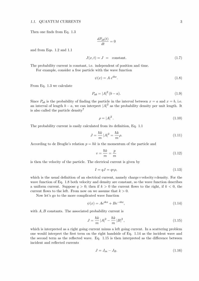
Figure 1.1: Cartoon representing a general one-dimenssional scattering problem. In the leftregion the potential is a constant V (x) = VL, in the middle region the potential V (x) can beanything, and in the right region the potential is a constant V (x) = VR. The middle region iscalled the scattering region. The left and right regions are called the left and right leads.In the left lead we have an incoming wave AeikLx and a reflected wave Be−ikLx and in the rightlead we have a transmitted wave FeikRx.
The reflection coefficient R is defined as the ratio between reflected and incident currents
R =JRJin
=|B|2|A|2 . (1.17)
Consider the scattering problem shown in Fig. 1.1. In the left region we assume that thepotential is constant V (x) = VL, in the middle region the potential can have any shape V (x),and in the right region the potential is again constant V (x) = VR. The solution in the left regionis given by Eq. 1.14 with k replaced by kL
kL =
p2m(E − VL)
h. (1.18)
The solution in the right region is given by the transmitted wave
ψ(x) = FeikRx ; x in right region, (1.19)
with
kR =
p2m(E − VR)
h. (1.20)
One can calculate the transmitted current as
JT =hkRm
|F |2 . (1.21)
The transmission coefficient T is defined as the ratio between transmitted and incident currents
T =JTJin
=vRvL
|F |2|A|2 , (1.22)
7Using a beam of N particles in which each particle is independent of the others and is described by the wavefunction of Eq. 1.8, the particle density is N |A|2, which is the number of particles to be found per unit length.
1.2. QUANTUM CONDUCTANCE 5
using Eq. 1.12.
From the fact that the current has to be independent of position everywhere, see Eq. 1.7, itfollows from Eqs. 1.16 and 1.21 that
Jin − JR = JT ⇔Jin = JR + JT . (1.23)
This relation expresses the conservation of current, or: “current in = current out” (reflectedplus transmitted). No matter how weird the potential in the middle region is, the current goinginto it has to be equal to the total current coming out of it. No particles magically appear ordisappear in the middle region. From the definitions of Eqs. 1.17 and 1.22 it is shown that Eq.1.23 is equivalent to
1 = R+ T, (1.24)
i.e. the reflection and transmission coefficients add up to 1. Since these coefficients denote theprobabilities that a particle is reflected or transmitted, this simply states that particles are eitherreflected or transmitted.
1.2 Quantum conductance
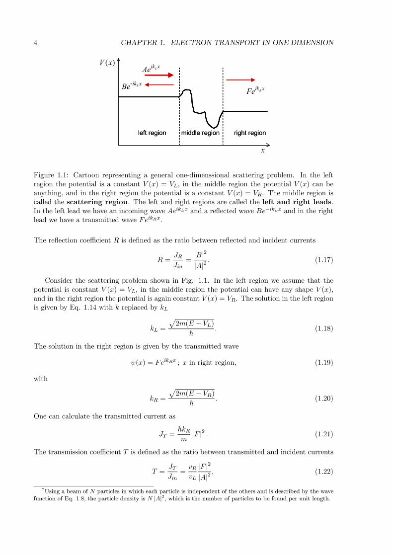
1.2.1 Tunnel junction
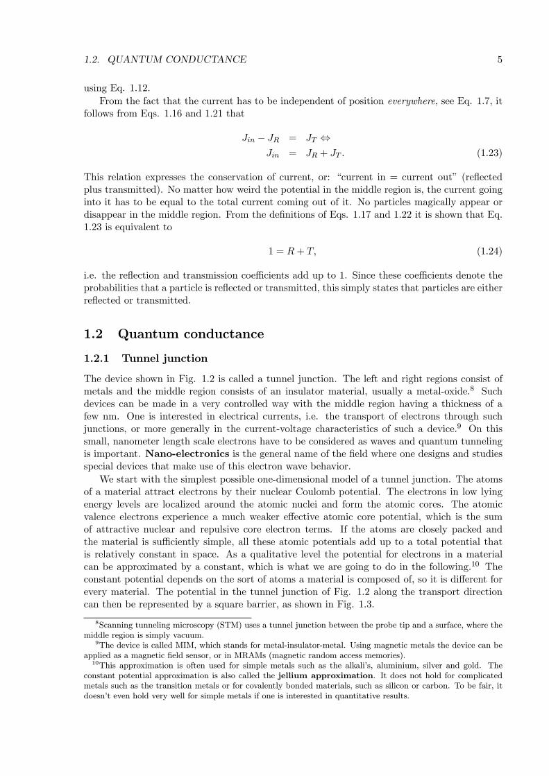
The device shown in Fig. 1.2 is called a tunnel junction. The left and right regions consist ofmetals and the middle region consists of an insulator material, usually a metal-oxide.8 Suchdevices can be made in a very controlled way with the middle region having a thickness of afew nm. One is interested in electrical currents, i.e. the transport of electrons through suchjunctions, or more generally in the current-voltage characteristics of such a device.9 On thissmall, nanometer length scale electrons have to be considered as waves and quantum tunnelingis important. Nano-electronics is the general name of the field where one designs and studiesspecial devices that make use of this electron wave behavior.
We start with the simplest possible one-dimensional model of a tunnel junction. The atomsof a material attract electrons by their nuclear Coulomb potential. The electrons in low lyingenergy levels are localized around the atomic nuclei and form the atomic cores. The atomicvalence electrons experience a much weaker effective atomic core potential, which is the sumof attractive nuclear and repulsive core electron terms. If the atoms are closely packed andthe material is sufficiently simple, all these atomic potentials add up to a total potential thatis relatively constant in space. As a qualitative level the potential for electrons in a materialcan be approximated by a constant, which is what we are going to do in the following.10 Theconstant potential depends on the sort of atoms a material is composed of, so it is different forevery material. The potential in the tunnel junction of Fig. 1.2 along the transport directioncan then be represented by a square barrier, as shown in Fig. 1.3.
8Scanning tunneling microscopy (STM) uses a tunnel junction between the probe tip and a surface, where themiddle region is simply vacuum.
9The device is called MIM, which stands for metal-insulator-metal. Using magnetic metals the device can beapplied as a magnetic field sensor, or in MRAMs (magnetic random access memories).10This approximation is often used for simple metals such as the alkali’s, aluminium, silver and gold. The
constant potential approximation is also called the jellium approximation. It does not hold for complicatedmetals such as the transition metals or for covalently bonded materials, such as silicon or carbon. To be fair, itdoesn’t even hold very well for simple metals if one is interested in quantitative results.
6 CHAPTER 1. ELECTRON TRANSPORT IN ONE DIMENSION
incoming wave
transmitted wavereflected wave
left region right regionmiddleregion
incoming wave
transmitted wavereflected wave
left region right regionmiddleregion
Figure 1.2: Schematic representation of a tunnel junction. The yellow balls represent atomsof a metal, the blue balls represent atoms of an insulator. The left and right regions stretchmacroscopically far into the left and right, respectively. The electron waves in the metal arereflected or transmitted by the insulator in the middle region
ikxAe
-ikxBeikxFe
( )V x
x
left region right regionmiddle region
ikxAe
-ikxBeikxFe
( )V x
x
left region right regionmiddle region
Figure 1.3: Simple approximation of the potential along the transport direction of a tunneljunction, see Fig. 1.2. In the metal (left and right regions) the potential is constant, V (x) = V1.In the insulator the potential is also constant, V (x) = V0, where V0 > V1. The incoming,reflected and transmitted waves are given by Aeikx, Be−ikx and Feikx.
1.2. QUANTUM CONDUCTANCE 7
( )V x
x
left region right regionmiddle region
1V
0V
0 − ∆V V
1 − ∆V V
( )V x
x
left region right regionmiddle region
1V
0V
0 − ∆V V
1 − ∆V V
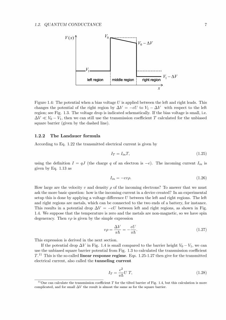
Figure 1.4: The potential when a bias voltage U is applied between the left and right leads. Thischanges the potential of the right region by ∆V = −eU to V1 − ∆V with respect to the leftregion; see Fig. 1.3. The voltage drop is indicated schematically. If the bias voltage is small, i.e.∆V ¿ V0 − V1, then we can still use the transmission coefficient T calculated for the unbiasedsquare barrier (given by the dashed line).
1.2.2 The Landauer formula
According to Eq. 1.22 the transmitted electrical current is given by
IT = IinT, (1.25)
using the definition I = qJ (the charge q of an electron is −e). The incoming current Iin isgiven by Eq. 1.13 as
Iin = −evρ. (1.26)
How large are the velocity v and density ρ of the incoming electrons? To answer that we mustask the more basic question: how is the incoming current in a device created? In an experimentalsetup this is done by applying a voltage difference U between the left and right regions. The leftand right regions are metals, which can be connected to the two ends of a battery, for instance.This results in a potential drop ∆V = −eU between left and right regions, as shown in Fig.1.4. We suppose that the temperature is zero and the metals are non-magnetic, so we have spindegeneracy. Then vρ is given by the simple expression
vρ =∆V
πh= −eU
πh. (1.27)
This expression is derived in the next section.
If the potential drop ∆V in Fig. 1.4 is small compared to the barrier height V0−V1, we canuse the unbiased square barrier potential from Fig. 1.3 to calculated the transmission coefficientT .11 This is the so-called linear response regime. Eqs. 1.25-1.27 then give for the transmittedelectrical current, also called the tunneling current
IT =e2
πhU T, (1.28)
11One can calculate the transmission coefficient T for the tilted barrier of Fig. 1.4, but this calculation is morecomplicated, and for small ∆V the result is almost the same as for the square barrier.
8 CHAPTER 1. ELECTRON TRANSPORT IN ONE DIMENSION
which is a remarkably simple expression! If we define the conductance G as current dividedby voltage, we get
G = ITU=e2
πhT. (1.29)
Since T is just a dimensionless number between 0 and 1, e2/πh has the dimension of conductance.It is the fundamental quantum of conductance; its value is e2/πh ≈ 7.75× 10⁻⁵ Ω−1.12
Eq. 1.29 is called the Landauer formula; it plays a central role in nano-electronics.13 Asit stands here, it is valid for a one-dimensional, spin degenerate system at low voltage and atnot too high a temperature, but it can be generalized.
1.2.3 Simple derivation of the Landauer formula
I will give a very simple derivation of Eq. 1.27. We have to do a little bit of solid state physics,but I use only simple introductory quantum mechanics language. Spin degeneracy means thateach energy level can be filled with two electrons. The non spin degenerate case is relevant formagnetic materials. I let you work out that case yourself.
The Pauli exclusion principle and the Fermi energy
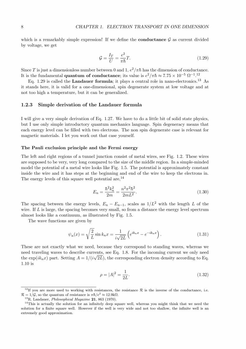
The left and right regions of a tunnel junction consist of metal wires, see Fig. 1.2. These wiresare supposed to be very, very long compared to the size of the middle region. In a simple-mindedmodel the potential of a metal wire looks like Fig. 1.5. The potential is approximately constantinside the wire and it has steps at the beginning and end of the wire to keep the electrons in.The energy levels of this square well potential are,14
En =h2k2n2m
=n2π2h2
2mL2. (1.30)
The spacing between the energy levels, En − En−1, scales as 1/L2 with the length L of thewire. If L is large, the spacing becomes very small, so from a distance the energy level spectrumalmost looks like a continuum, as illustrated by Fig. 1.5.
The wave functions are given by
ψn(x) =
r2
Lsin knx =
1
i√2L
³eiknx − e−iknx
´. (1.31)
These are not exactly what we need, because they correspond to standing waves, whereas weneed traveling waves to describe currents, see Eq. 1.8. For the incoming current we only needthe exp(iknx) part. Setting A = 1/(i
√2L), the corresponding electron density according to Eq.
1.10 is
ρ = |A|2 = 1
2L. (1.32)
12If you are more used to working with resistances, the resistance R is the inverse of the conductance, i.e.R = 1/G, so the quantum of resistance is πh/e2 ≈ 12.9kΩ.13R. Landauer, Philosophical Magazine 21, 863 (1970).14This is actually the solution for an infinitely deep square well, whereas you might think that we need the
solution for a finite square well. However if the well is very wide and not too shallow, the infinite well is anextremely good approximation.
1.2. QUANTUM CONDUCTANCE 9
( )V x
x
FE
2L
2−L
( )V x
x
FE
2L
2−L
Figure 1.5: Schematic drawing of the potential and the energy levels of a long wire. The points−L/2 and L/2 mark the beginning and the end of the wire. The spacing between the energylevels is so small that the energy spectrum almost looks like a continuum. EF marks the Fermienergy, i.e. the highest level that is occupied in the ground state by an electron.
The wire is full of electrons since each of the atoms in the wire brings at least one electronwith it. Filling the energy levels according to the Pauli principle, and having N electrons intotal, the highest occupied level is EN
2. The highest occupied level in the ground state is called
the Fermi energy or EF .15
Incoming and tunnel currents
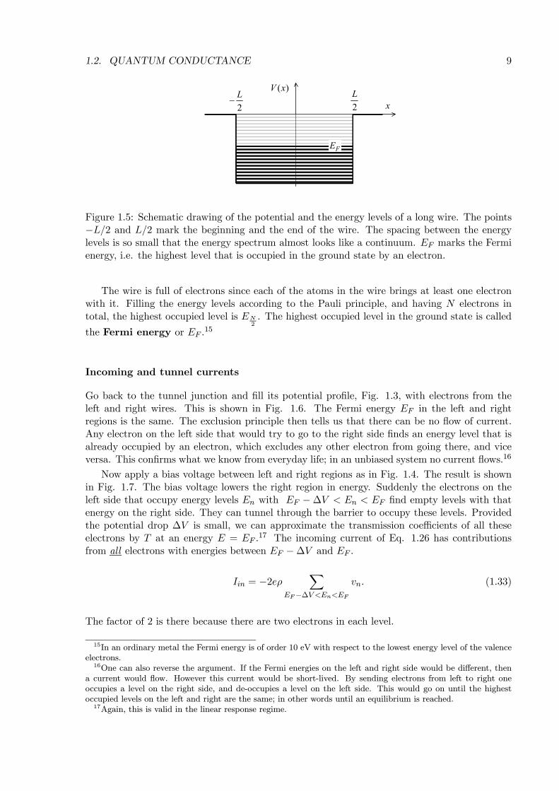
Go back to the tunnel junction and fill its potential profile, Fig. 1.3, with electrons from theleft and right wires. This is shown in Fig. 1.6. The Fermi energy EF in the left and rightregions is the same. The exclusion principle then tells us that there can be no flow of current.Any electron on the left side that would try to go to the right side finds an energy level that isalready occupied by an electron, which excludes any other electron from going there, and viceversa. This confirms what we know from everyday life; in an unbiased system no current flows.16
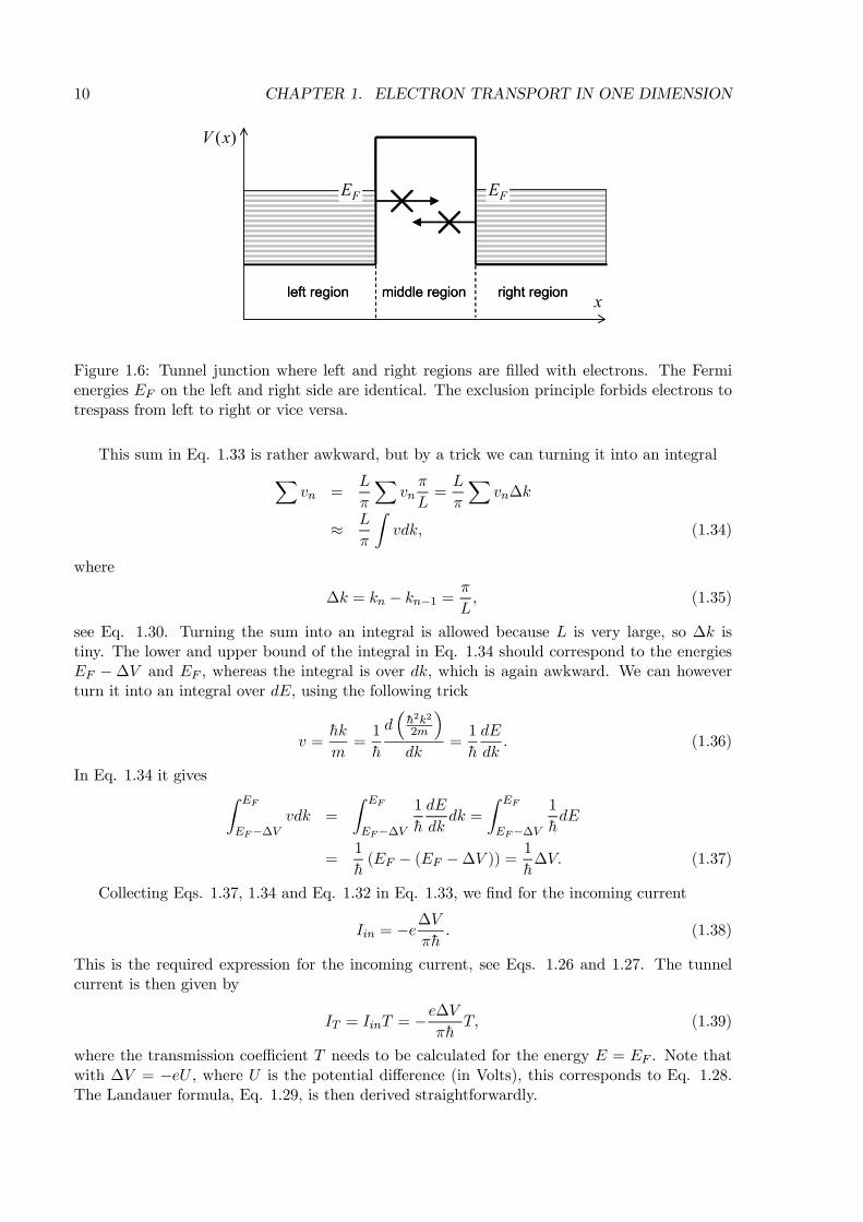
Now apply a bias voltage between left and right regions as in Fig. 1.4. The result is shownin Fig. 1.7. The bias voltage lowers the right region in energy. Suddenly the electrons on theleft side that occupy energy levels En with EF −∆V < En < EF find empty levels with thatenergy on the right side. They can tunnel through the barrier to occupy these levels. Providedthe potential drop ∆V is small, we can approximate the transmission coefficients of all theseelectrons by T at an energy E = EF .
17 The incoming current of Eq. 1.26 has contributionsfrom all electrons with energies between EF −∆V and EF .
Iin = −2eρX
EF−∆V <En<EFvn. (1.33)
The factor of 2 is there because there are two electrons in each level.
15In an ordinary metal the Fermi energy is of order 10 eV with respect to the lowest energy level of the valenceelectrons.16One can also reverse the argument. If the Fermi energies on the left and right side would be different, then
a current would flow. However this current would be short-lived. By sending electrons from left to right oneoccupies a level on the right side, and de-occupies a level on the left side. This would go on until the highestoccupied levels on the left and right are the same; in other words until an equilibrium is reached.17Again, this is valid in the linear response regime.
10 CHAPTER 1. ELECTRON TRANSPORT IN ONE DIMENSION
( )V x
xleft region right regionmiddle region
FEFE
( )V x
xleft region right regionmiddle region
FEFE
Figure 1.6: Tunnel junction where left and right regions are filled with electrons. The Fermienergies EF on the left and right side are identical. The exclusion principle forbids electrons totrespass from left to right or vice versa.
This sum in Eq. 1.33 is rather awkward, but by a trick we can turning it into an integralXvn =
L
π
Xvn
π
L=L
π
Xvn∆k
≈ L
π
Zvdk, (1.34)
where
∆k = kn − kn−1 = π
L, (1.35)
see Eq. 1.30. Turning the sum into an integral is allowed because L is very large, so ∆k istiny. The lower and upper bound of the integral in Eq. 1.34 should correspond to the energiesEF −∆V and EF , whereas the integral is over dk, which is again awkward. We can howeverturn it into an integral over dE, using the following trick
v =hk
m=1
h
d³h2k2
2m
´dk
=1
h
dE
dk. (1.36)
In Eq. 1.34 it gives Z EF
EF−∆Vvdk =
Z EF
EF−∆V1
h
dE
dkdk =
Z EF
EF−∆V1
hdE
=1
h(EF − (EF −∆V )) = 1
h∆V. (1.37)
Collecting Eqs. 1.37, 1.34 and Eq. 1.32 in Eq. 1.33, we find for the incoming current
Iin = −e∆Vπh
. (1.38)
This is the required expression for the incoming current, see Eqs. 1.26 and 1.27. The tunnelcurrent is then given by
IT = IinT = −e∆Vπh
T, (1.39)
where the transmission coefficient T needs to be calculated for the energy E = EF . Note thatwith ∆V = −eU , where U is the potential difference (in Volts), this corresponds to Eq. 1.28.The Landauer formula, Eq. 1.29, is then derived straightforwardly.
1.3. TRANSFER AND SCATTERING MATRICES 11
( )V x
xleft region right regionmiddle region
0V
0 − ∆V V
FE− ∆FE V
( )V x
xleft region right regionmiddle region
0V
0 − ∆V V
FE− ∆FE V
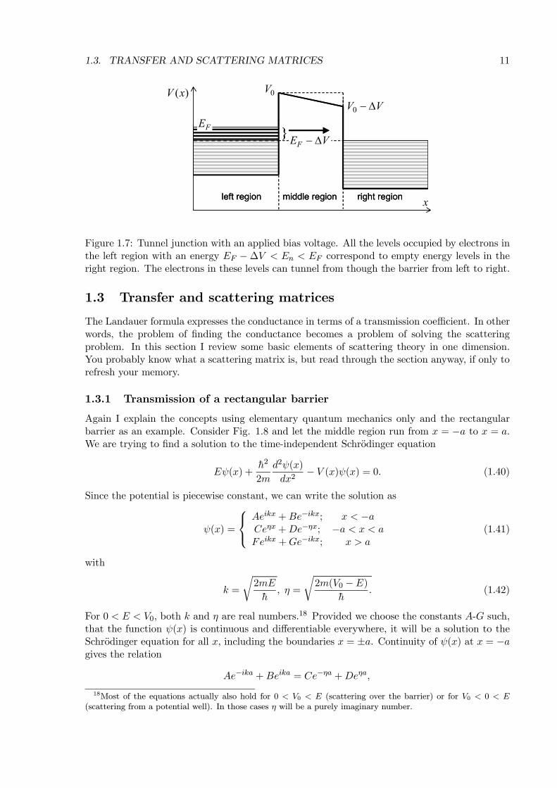
Figure 1.7: Tunnel junction with an applied bias voltage. All the levels occupied by electrons inthe left region with an energy EF −∆V < En < EF correspond to empty energy levels in theright region. The electrons in these levels can tunnel from though the barrier from left to right.
1.3 Transfer and scattering matrices
The Landauer formula expresses the conductance in terms of a transmission coefficient. In otherwords, the problem of finding the conductance becomes a problem of solving the scatteringproblem. In this section I review some basic elements of scattering theory in one dimension.You probably know what a scattering matrix is, but read through the section anyway, if only torefresh your memory.
1.3.1 Transmission of a rectangular barrier
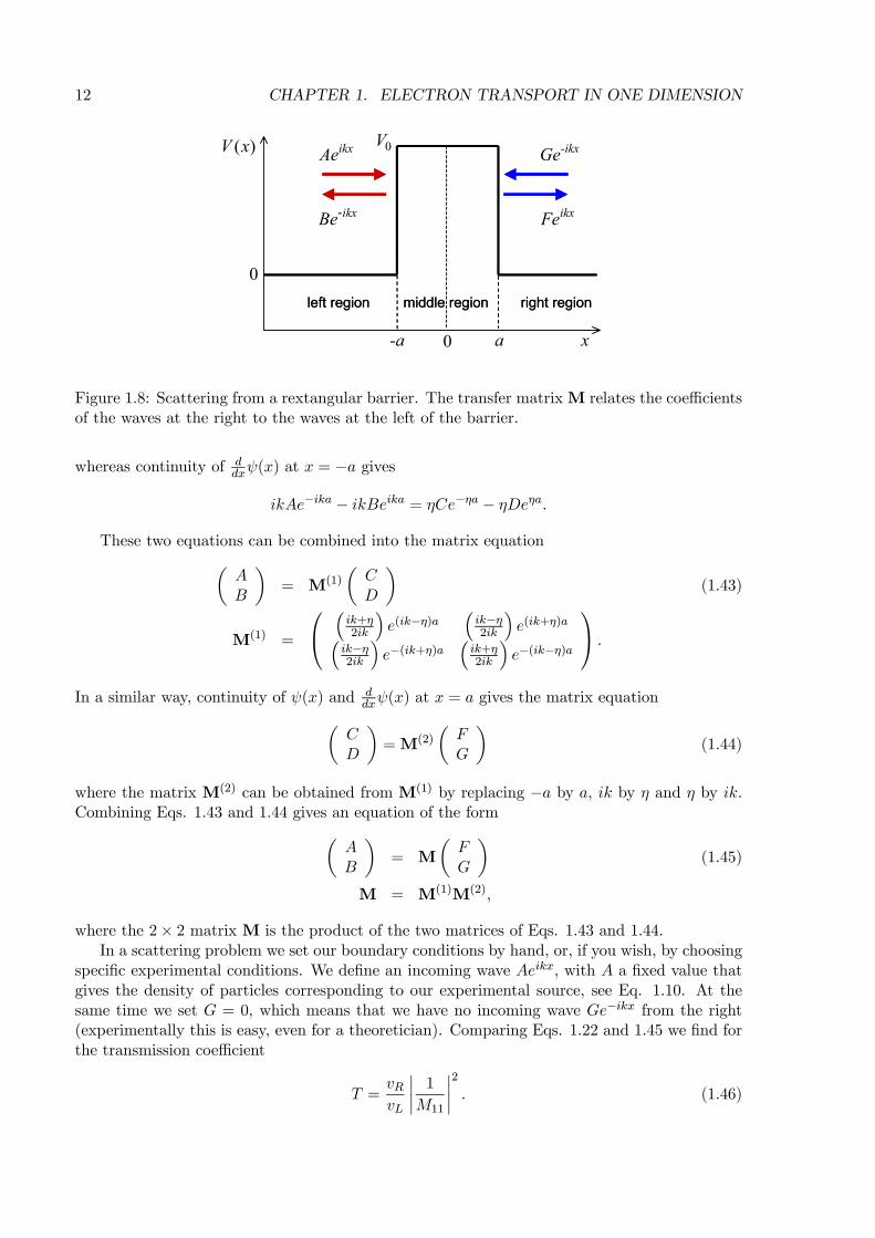
Again I explain the concepts using elementary quantum mechanics only and the rectangularbarrier as an example. Consider Fig. 1.8 and let the middle region run from x = −a to x = a.We are trying to find a solution to the time-independent Schrodinger equation
Eψ(x) +h2
2m
d2ψ(x)
dx2− V (x)ψ(x) = 0. (1.40)
Since the potential is piecewise constant, we can write the solution as
ψ(x) =
Aeikx +Be−ikx; x < −aCeηx +De−ηx; −a < x < aFeikx +Ge−ikx; x > a
(1.41)
with
k =
r2mE
h, η =
r2m(V0 −E)
h. (1.42)
For 0 < E < V0, both k and η are real numbers.18 Provided we choose the constants A-G such,that the function ψ(x) is continuous and differentiable everywhere, it will be a solution to theSchrodinger equation for all x, including the boundaries x = ±a. Continuity of ψ(x) at x = −agives the relation
Ae−ika +Beika = Ce−ηa +Deηa,18Most of the equations actually also hold for 0 < V0 < E (scattering over the barrier) or for V0 < 0 < E
(scattering from a potential well). In those cases η will be a purely imaginary number.
12 CHAPTER 1. ELECTRON TRANSPORT IN ONE DIMENSION
ikxAe
-ikxBe ikxFe
( )V x
x
left region right regionmiddle region
-ikxGe
a-a 0
0
0VikxAe
-ikxBe ikxFe
( )V x
x
left region right regionmiddle region
-ikxGe
a-a 0
0
0V
Figure 1.8: Scattering from a rextangular barrier. The transfer matrixM relates the coefficientsof the waves at the right to the waves at the left of the barrier.
whereas continuity of ddxψ(x) at x = −a gives
ikAe−ika − ikBeika = ηCe−ηa − ηDeηa.
These two equations can be combined into the matrix equationµAB
¶= M(1)
µCD
¶(1.43)
M(1) =
³ik+η2ik
´e(ik−η)a
³ik−η2ik
´e(ik+η)a³
ik−η2ik
´e−(ik+η)a
³ik+η2ik
´e−(ik−η)a
.In a similar way, continuity of ψ(x) and d
dxψ(x) at x = a gives the matrix equationµCD
¶=M(2)
µFG
¶(1.44)
where the matrix M(2) can be obtained from M(1) by replacing −a by a, ik by η and η by ik.Combining Eqs. 1.43 and 1.44 gives an equation of the formµ
AB
¶= M
µFG
¶(1.45)
M = M(1)M(2),
where the 2× 2 matrix M is the product of the two matrices of Eqs. 1.43 and 1.44.In a scattering problem we set our boundary conditions by hand, or, if you wish, by choosing
specific experimental conditions. We define an incoming wave Aeikx, with A a fixed value thatgives the density of particles corresponding to our experimental source, see Eq. 1.10. At thesame time we set G = 0, which means that we have no incoming wave Ge−ikx from the right(experimentally this is easy, even for a theoretician). Comparing Eqs. 1.22 and 1.45 we find forthe transmission coefficient
T =vRvL
¯1
M11
¯2. (1.46)

1.3. TRANSFER AND SCATTERING MATRICES 13
Lik xAe- Lik xBe
Rik xFe
( )V x
x
left region right region
1x ix Nx
potential barrier
Lik xAe- Lik xBe
Rik xFe
( )V x
x
left region right region
1x ix Nx
potential barrier
Figure 1.9: Approximating a barrier of any shape by a series of steps. The transfer matrix Mis given byM =M1M1 · · ·MN .
Since the potential is symmetric, we actually have vR = vL here, but we let the more generalform of Eq. 1.46 stand for later. It is a simple exercise to work out the matrix element M11 andshow that one obtains the usual textbook expression for the transmission coefficient
T =
·1 +
µk2 + η2
2kη
¶sinh2(2ηa)
¸−1. (1.47)
Comparing Eqs. 1.17 and 1.45 gives the reflection coefficient as
R =|M21|2|M11|2
. (1.48)
1.3.2 Transmission of a general barrier
The algorithm formulated in the previous section can be extended in order to describe thetransmission through a barrier of a more general shape. The matrix M as in Eq. 1.45 is calledthe transfer matrix. It relates the modes in the right region to the modes in the left region.Once we know the transfer matrix, we can calculate the reflection and transmission coefficients,see Eqs. 1.48 and 1.46. For a single step in the potential, the transfer matrices are given byEqs. 1.43 and 1.44 for a step up and a step down, respectively. Since the square barrier can beviewed as a step up (at x = −a), followed by step down (at x = a), its transfer matrix is simplya product of the transfer matrices of the individual steps, as is expressed by Eq. 1.45. The ideacan be applied to a potential of any shape, approximating the potential by a series of steps, asis illustrated in Fig. 1.9.
The transfer matrixM is given by the product of the transfer matrices of each step
M =M1M1 · · ·MN , (1.49)
where each Mi can be calculated by defining
ηi =
p2m [V (xi)−E]
h, (1.50)
and using a properly modified Eq. 1.43 or Eq. 1.44. I leave the details up to you. In essence thisis the transfer matrix algorithm. It is used quite frequently in numerical calculations solving
14 CHAPTER 1. ELECTRON TRANSPORT IN ONE DIMENSION
scattering problems in various branches of physics; quantum mechanics, optics, acoustics, etc..Obviously it is best suited for layered materials, i.e. systems that consist of layers of differentmaterials stacked on top of one another. If the ηi get large, which is for high barriers and/orlow energies, one might get into numerical problems because of the exponentials in Eqs. 1.43and 1.44. There are some special tricks to handle these, but I won’t go into details here. Forsystems described in terms of real atoms, the techniques discussed in the following sections arebetter suited.
1.3.3 The scattering or S matrix
The transfer matrix M is closely related to an elementary concept in scattering theory, calledthe scattering matrix. Whereas the transfer matrix relates the modes on the right to the modeson the left, the scattering matrix relates outgoing modes to incoming modes. For the exampleshown in Fig. 1.8, the modes that are coming into the barrier are Aeikx (from the left) andGe−ikx (from the right) and the modes that are going out from the barrier are Be−ikx (to theleft) and Feikx (to the right). The scattering matrix is defined by the relationµ
BF
¶= S0
µAG
¶. (1.51)
Comparison to Eq. 1.45 gives for its matrix elements
S011 =M21
M11; S012 =M22 −M21
M12
M11;
S021 =1
M11; S022 = −
M12
M11. (1.52)
I have put a “prime” on S0 because the scattering matrix S as it ordinarily used is defined as
S11 = S011; S12 =rvLvRS012;
S21 =
rvRvLS021; S22 = S
022. (1.53)
The reason for introducing the√v factors is because one wants the scattering matrix S to
reflect a basic conservation law, namely the conservation of current. In a stationary problemthe current going out must be the same as the current coming in, since otherwise one would getan accumulation or depletion of particles, as discussed Sec. 1.1.
Jout = Jin ⇒vL |B|2 + vR |F |2 = vL |A|2 + vR |G|2 ⇒°°°°µ √vLB√
vRF
¶°°°°2 =
°°°°µ √vLA√vRG
¶°°°°2 . (1.54)
From Eqs. 1.51 and 1.53 it is easily shown that this holds only if
S†S = SS† = 1. (1.55)
In other words, conservation of current means that the scattering matrix is unitary.It is custom to write the scattering matrix as
S =
µr t0
t r0
¶. (1.56)
1.4. MODE MATCHING 15
Lik xAe- Lik xBe
Rik xFe
( )V x
x
left region right region
1x ix Nx0x N+1x
potential barrier
∆
Lik xAe- Lik xBe
Rik xFe
( )V x
x
left region right region
1x ix Nx0x N+1x
potential barrier
∆
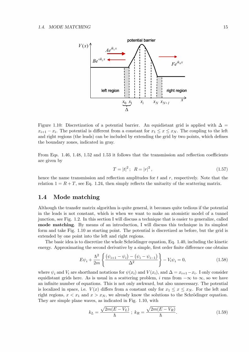
Figure 1.10: Discretization of a potential barrier. An equidistant grid is applied with ∆ =xi+1 − xi. The potential is different from a constant for x1 ≤ x ≤ xN . The coupling to the leftand right regions (the leads) can be included by extending the grid by two points, which definesthe boundary zones, indicated in gray.
From Eqs. 1.46, 1.48, 1.52 and 1.53 it follows that the transmission and reflection coefficientsare given by
T = |t|2 ; R = |r|2 , (1.57)
hence the name transmission and reflection amplitudes for t and r, respectively. Note that therelation 1 = R+ T , see Eq. 1.24, then simply reflects the unitarity of the scattering matrix.
1.4 Mode matching
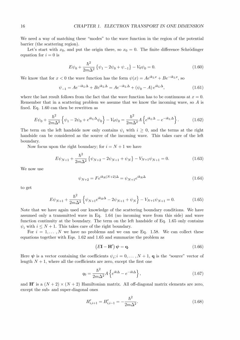
Although the transfer matrix algorithm is quite general, it becomes quite tedious if the potentialin the leads is not constant, which is when we want to make an atomistic model of a tunneljunction, see Fig. 1.2. In this section I will discuss a technique that is easier to generalize, calledmode matching. By means of an introduction, I will discuss this technique in its simplestform and take Fig. 1.10 as starting point. The potential is discretized as before, but the grid isextended by one point into the left and right regions.
The basic idea is to discretize the whole Schrodinger equation, Eq. 1.40, including the kineticenergy. Approximating the second derivative by a simple, first order finite difference one obtains
Eψi +h2
2m
(¡ψi+1 − ψi
¢− ¡ψi − ψi−1¢
∆2
)− Viψi = 0, (1.58)
where ψi and Vi are shorthand notations for ψ(xi) and V (xi), and ∆ = xi+1−xi. I only considerequidistant grids here. As is usual in a scattering problem, i runs from −∞ to ∞, so we havean infinite number of equations. This is not only awkward, but also unnecessary. The potentialis localized in space, i.e. V (x) differs from a constant only for x1 ≤ x ≤ xN . For the left andright regions, x < x1 and x > xN , we already know the solutions to the Schrodinger equation.They are simple plane waves, as indicated in Fig. 1.10, with
kL =
p2m(E − VL)
h; kR =
p2m(E − VR)
h. (1.59)
16 CHAPTER 1. ELECTRON TRANSPORT IN ONE DIMENSION
We need a way of matching these “modes” to the wave function in the region of the potentialbarrier (the scattering region).
Let’s start with x0, and put the origin there, so x0 = 0. The finite difference Schrodingerequation for i = 0 is
Eψ0 +h2
2m∆2©ψ1 − 2ψ0 + ψ−1
ª− V0ψ0 = 0. (1.60)
We know that for x < 0 the wave function has the form ψ(x) = AeikLx +Be−ikLx, so
ψ−1 = Ae−ikL∆ +BeikL∆ = Ae−ikL∆ + (ψ0 −A) eikL∆, (1.61)
where the last result follows from the fact that the wave function has to be continuous at x = 0.Remember that in a scattering problem we assume that we know the incoming wave, so A isfixed. Eq. 1.60 can then be rewritten as
Eψ0 +h2
2m∆2
nψ1 − 2ψ0 + eikL∆ψ0
o− V0ψ0 =
h2
2m∆2AneikL∆ − e−ikL∆
o. (1.62)
The term on the left handside now only contains ψi with i ≥ 0, and the terms at the righthandside can be considered as the source of the incoming wave. This takes care of the leftboundary.
Now focus upon the right boundary; for i = N + 1 we have
EψN+1 +h2
2m∆2©ψN+2 − 2ψN+1 + ψN
ª− VN+1ψN+1 = 0. (1.63)
We now use
ψN+2 = FeikR(N+2)∆ = ψN+1e
ikR∆ (1.64)
to get
EψN+1 +h2
2m∆2
nψN+1e
ikR∆ − 2ψN+1 + ψN
o− VN+1ψN+1 = 0. (1.65)
Note that we have again used our knowledge of the scattering boundary conditions. We haveassumed only a transmitted wave in Eq. 1.64 (no incoming wave from this side) and wavefunction continuity at the boundary. The term on the left handside of Eq. 1.65 only containsψi with i ≤ N + 1. This takes care of the right boundary.
For i = 1, . . . , N we have no problems and we can use Eq. 1.58. We can collect theseequations together with Eqs. 1.62 and 1.65 and summarize the problem as¡
EI−H0¢ψ = q. (1.66)
Here ψ is a vector containing the coefficients ψi; i = 0, . . . , N + 1, q is the “source” vector oflength N + 1, where all the coefficients are zero, except the first one
q0 =h2
2m∆2Aneik∆ − e−ik∆
o, (1.67)
and H0 is a (N + 2) × (N + 2) Hamiltonian matrix. All off-diagonal matrix elements are zero,except the sub- and super-diagonal ones
H 0i,i+1 = H
0i,i−1 = −
h2
2m∆2. (1.68)
1.4. MODE MATCHING 17
All diagonal matrix elements are identical to that of the original finite difference Hamiltonian
H 0i,i = −
h2
m∆2+ Vi, (1.69)
except the first and the last one, which are modified to
H 00,0 = − h2
m∆2+ V0 +ΣL(E),
H 0N+1,N+1 = − h2
m∆2+ VN+1 +ΣR(E). (1.70)
with
ΣL(E) = − h2
2m∆2eikL∆,
ΣR(E) = − h2
2m∆2eikR∆. (1.71)
The quantities ΣL/R(E) are called the self-energies of the left and right leads.19 They take
care of the proper coupling of the potential barrier to the outer regions, and contain all theinformation we require about the outer regions. The self-energy depends upon the energy of theincoming and scattered waves, see Eq. 1.59. Note that, while Eq. 1.58 represents an infinitedimensional problem, by introducing the self-energy (and the source), we have reduced it to afinite, N +2 dimensional problem, Eq. 1.66. That can be solved using standard algorithmsfor solving linear equations.20
Once you have solved Eq. 1.66, the only thing remaining is to extract the transmission andreflection amplitudes. The transmission amplitude is simply given by the wave function at theright side of the barrier, normalized to the incoming wave, and normalized with the velocities(to attain a unitary scattering matrix, see Eq. 1.53)
t =
rvRvL
ψN+1A
. (1.72)
The reflection amplitude is similarly determined from the wave function on the left side minusthe incoming wave, normalized to the incoming wave
r =ψ0 −AA
. (1.73)
Some care should be taken in determining the velocities. Since we have discretized theSchrodinger equation, it is consistent to discretize the expression for the current, Eq. 1.1, in asimilar way
J =ih
2m
µψi
ψ∗i+1 − ψ∗i∆
− ψ∗iψi+1 − ψi∆
¶. (1.74)
This should actually give a position independent result, since we are considering a stationaryproblem. For a simple plane wave Aeikx this expression gives
J =ih |A|22m∆
³e−ik∆ − eik∆
´,
19a somewhat unfortunate term descending from Green function folklore.20In this case it is particularly simple, since the matrix is tridiagonal.

18 CHAPTER 1. ELECTRON TRANSPORT IN ONE DIMENSION
and comparison to Eqs. 1.11 and 1.12 gives
v =ih
2m∆
³e−ik∆ − eik∆
´. (1.75)
Note that the continuum limit lim∆→0 of this expression gives Eq. 1.12.The source term, Eq. 1.67, can then be simplified to
q0 =ihA
∆vL. (1.76)
In addition, from Eqs. 1.75 and 1.71 one can relate the velocity to the self-energy
vL/R = −2∆
hImΣL/R(E). (1.77)
1.4.1 Green function expressions
Using Green functions the mode matching results can be put into a very compact, albeit some-what obscure, form. Define a matrix
G(E)=¡EI−H0¢−1 . (1.78)
It is called a Green-function matrix. Note that it has a dimension N +2, as has the modifiedHamiltonian matrix H0. One can also define the infinite dimensional retarded Green-functionmatrix related to the original infinite dimensional Hamiltonian
Gr(E)= [(E + iη)I−H]−1 , (1.79)
where η is (real, positive) infinitesimal. The advanced Green-function matrix is defined as21
Ga(E) = [Gr(E)]† . (1.80)
For z a complex number in the lower half plane, the matrix elements of G and Gr in thescattering region are identical.
Gi,j(z) = Gri,j(z) ; i, j = 0, . . . , N + 1 (1.81)
A proof of this can be found in the literature. Note that the modified Hamiltonian matrix H0
is non-Hermitian, essentially because the self-energy Σ is not real, see Eqs. 1.70 and 1.71. Onecan show that the eigenvalues of H0 are not real and lie in the upper half complex plane. Thus,G(E) is a well-defined quantity for real energies E (unlike Gr). It has the retarded boundarycondition build into it and one does not need the +iη trick.22
The definition of G allows us to write,
ψN+1 = GN+1,0(E)q0, (1.82)
21Since E is an eigenvalue of H, EI − H is singular and its inverse does not exist for real energies E.Adding/subtracting an imaginary iη avoids the singularities. In textbooks on scattering theory it is shown thatthis has a physical meaning. Gr can be used to construct the retarded wave function, which consists of a wavecoming in from the source to the target, and waves scattered out from the target. This is the physical solution.Ga gives the reverse, i.e. waves scattered into the target, plus waves going into the source. This is unphysical,but can sometimes be useful in formal mathematical manipulations. After having constructed the wave function,the linit limη→0 can be taken, so η only serves as an intermediate to reflect the boundary conditions.22Mathematicians would callG(E) an analytical continuation ofGr(E). All the poles of G(E) are in the upper
half plane, which makes it analytical on the real axis, and a retarded form.
1.4. MODE MATCHING 19
see Eq. 1.66. Eqs. 1.72, 1.76 and 1.82 then lead to a compact expression for the transmissionamplitude
t =ih
∆
√vRvL GN+1,0(E). (1.83)
An expression of this type is called a Fisher-Lee expression. It relates matrix elements of thescattering matrix to matrix elements of the Green function.
For Green function junkies, we can even make it fancier and write, using Eq. 1.77
t = 2ip− ImΣR GN+1,0(E)
p− ImΣL. (1.84)
This allows the transmission coefficient to be written as
T = t∗t = 4(ImΣR)GrN+1,0(ImΣL)Ga0,N+1 (1.85)
with all quantities evaluated at the fixed energy E. This expression is known as the Caroliexpression.
Introducing a Green function to tackle this simple one-dimensional problem is like using asledgehammer to crack a nut. Green functions expressions can however be modified to includemultiple dimensions, a large bias voltage, interactions with vibrations and/or between electrons,etc., where they give compact (though not necessarily practical) expressions. In case of a largebias voltage, the Caroli expression is also known as theNEGF expression, where NEGF standsfor non-equilibrium Green function.23
1.4.2 The embedding potential
If you prefer differential equations over linear algebra, we can take the continuum limit of Eq.1.66, i.e. lim∆→0. It is tricky, but straightforward to obtain
Eψ(x) +h2
2m
µd2ψ(x)
dx2+ δ(x)
dψ(x)
dx− δ(x− a)dψ(x)
dx
¶(1.86)
−V (x)ψ(x)− δ(x)ΣL(E) + δ(x− a)ΣR(E)ψ(x) = ihvLAδ(x),
where I have put the left boundary at x = 0 and the right boundary at x = a. The Σ’s have theform
ΣL/R(E) = −ihvL/R
2. (1.87)
The term on the right handside of Eq. 1.86 describes the source term, which only exists at theleft boundary. On the left handside there are δ-function terms that only exists at the boundariesof the barrier with the outside regions. They take care of the coupling to the outside region.The d
dx terms in the kinetic energy ensure a continuous derivative across the boundaries. Thepotential term between is called the embedding potential. The formalism is known in theliterature as the embedding formalism.24 The differential equation needs to be solved for ψ(x),but only over the finite domain 0 ≤ x ≤ a. The coupling to the outside regions is taken careof by the boundary terms. Eqs. 1.72 and 1.73 give the transmission and reflection amplitudeswith ψ(a) replacing ψN+1 and ψ(0) replacing ψ0.
23This is in contrast to the linear response regime, where the Green functions are ordinary, i.e. equilibriumGreen functions.24Be careful however, as in different fields the phrase “embedding” is attached to different things.

20 CHAPTER 1. ELECTRON TRANSPORT IN ONE DIMENSION
Alternatively, one may use Green function expressions also in this case. Define the Greenfunction G(x, x0, E) as the solution of the equation³
E − bH 0´G(x, x0, E) = δ(x− x0), (1.88)
where bH 0 is the operator of Eq. 1.86 including all potential and boundary terms. One can provethat G(x, x0, E) corresponds to the usual retarded Green function Gr for 0 ≤ x, x0 ≤ a.25 Thecontinuum equivalents of Eqs. 1.82-1.85 are
ψ(a) = G(a, 0, E)ihvLA,
t = ih√vRvL G(a, 0, E) = 2i
p− ImΣR G(a, 0, E)
p− ImΣL,
T = 4 ImΣRGr(a, 0, E) ImΣLG
a(0, a, E). (1.89)
I prefer linear algebra over differential equations and I don’t have experience with the embed-ding formalism, so it won’t be discussed further. It has been proven however that the formalismcan be extended into a practical method for calculating transport through small systems, in-cluding all atomic details.
1.5 Tight-binding
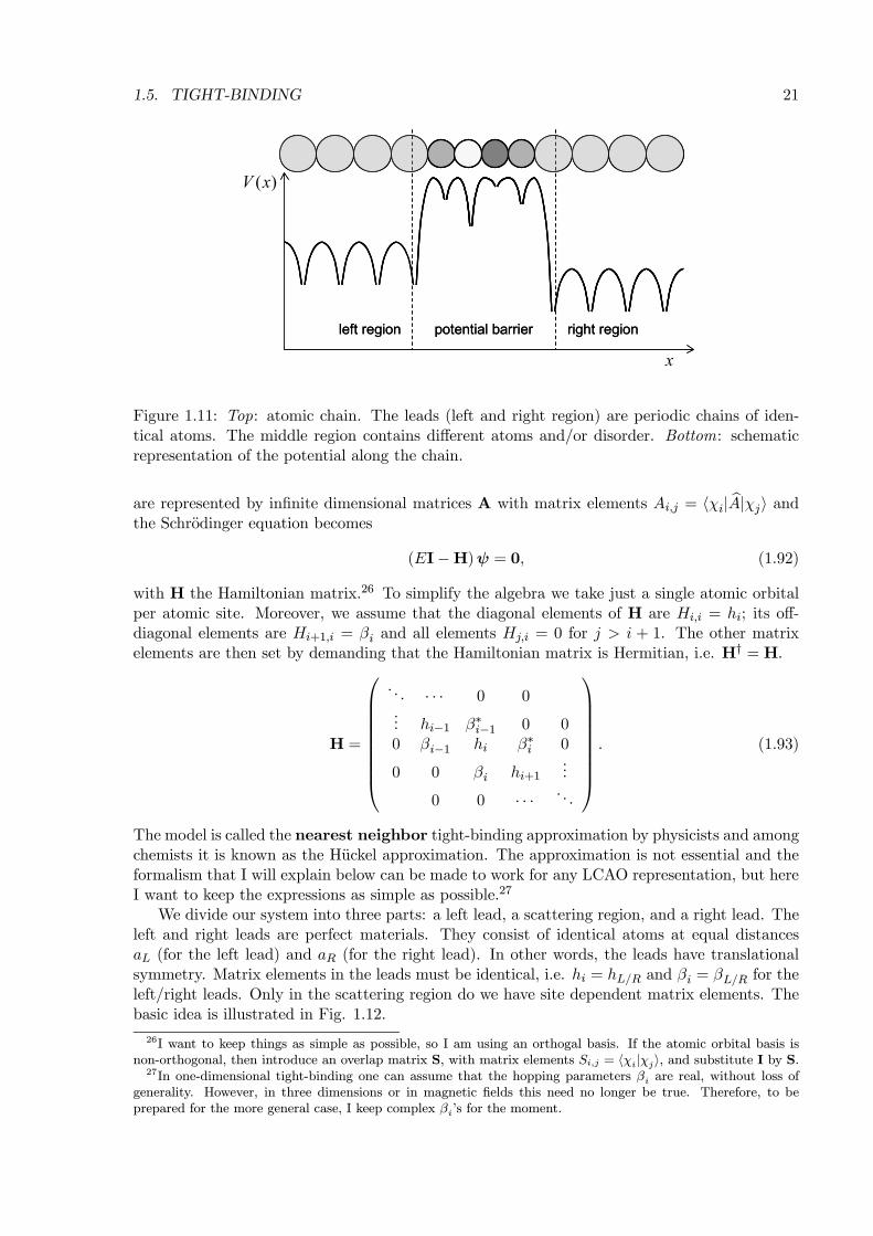
In previous sections we have analyzed one-dimensional scattering problems starting from po-tentials and wave functions as functions of a continuous coordinate. We have discretized thisrepresentation to show how the scattering problem can be solved in a practical way. This ap-proach is natural if the potential variation is confined to the scattering region and outside thisregion the potential is constant. The incoming, reflected and transmitted waves are then simplyplane waves. With the tunnel junction in mind, see Fig. 1.2, we would like to consider thesituation in which the whole space is filled with atoms of one kind or another. In one dimensionthis gives an atomic wire, with atomic potentials everywhere along the wire, as is illustrated inFig. 1.11.
The usual approach is to construct a representation on a basis of atomic orbitals, i.e. expandthe wave functions in fixed atomic orbitals χi(x)
ψ(x) =Xi
ciχi(x−Xi), (1.90)
where Xi denote the positions of the atoms. In chemistry this is known as the LCAO represen-tation (linear combination of atomic orbitals), in physics it is usually called the tight-bindingrepresentation. The wave function is represented by the column vector of the coefficients
ψ =
...ci−1cici+1...
. (1.91)
Since we want to solve a scattering problem, the atomic orbitals should cover all of (one-dimensional) space, so the vector has an infinite dimension, i.e. i = −∞, . . . ,∞. Operators bA25Gr(x, x0, E) is defined by
³E + iη − bH´Gr(x, x0, E) = δ(x−x0), for−∞ ≤ x, x0 ≤ ∞, with bH the Hamiltonian
without the boundary terms.
1.5. TIGHT-BINDING 21
( )V x
x
left region right regionpotential barrier
( )V x
x
left region right regionpotential barrier
Figure 1.11: Top: atomic chain. The leads (left and right region) are periodic chains of iden-tical atoms. The middle region contains different atoms and/or disorder. Bottom: schematicrepresentation of the potential along the chain.
are represented by infinite dimensional matrices A with matrix elements Ai,j = hχi| bA|χji andthe Schrodinger equation becomes
(EI−H)ψ = 0, (1.92)
with H the Hamiltonian matrix.26 To simplify the algebra we take just a single atomic orbitalper atomic site. Moreover, we assume that the diagonal elements of H are Hi,i = hi; its off-diagonal elements are Hi+1,i = βi and all elements Hj,i = 0 for j > i + 1. The other matrixelements are then set by demanding that the Hamiltonian matrix is Hermitian, i.e. H† = H.
H =
. . . · · · 0 0... hi−1 β∗i−1 0 00 βi−1 hi β∗i 0
0 0 βi hi+1...
0 0 · · · . . .
. (1.93)
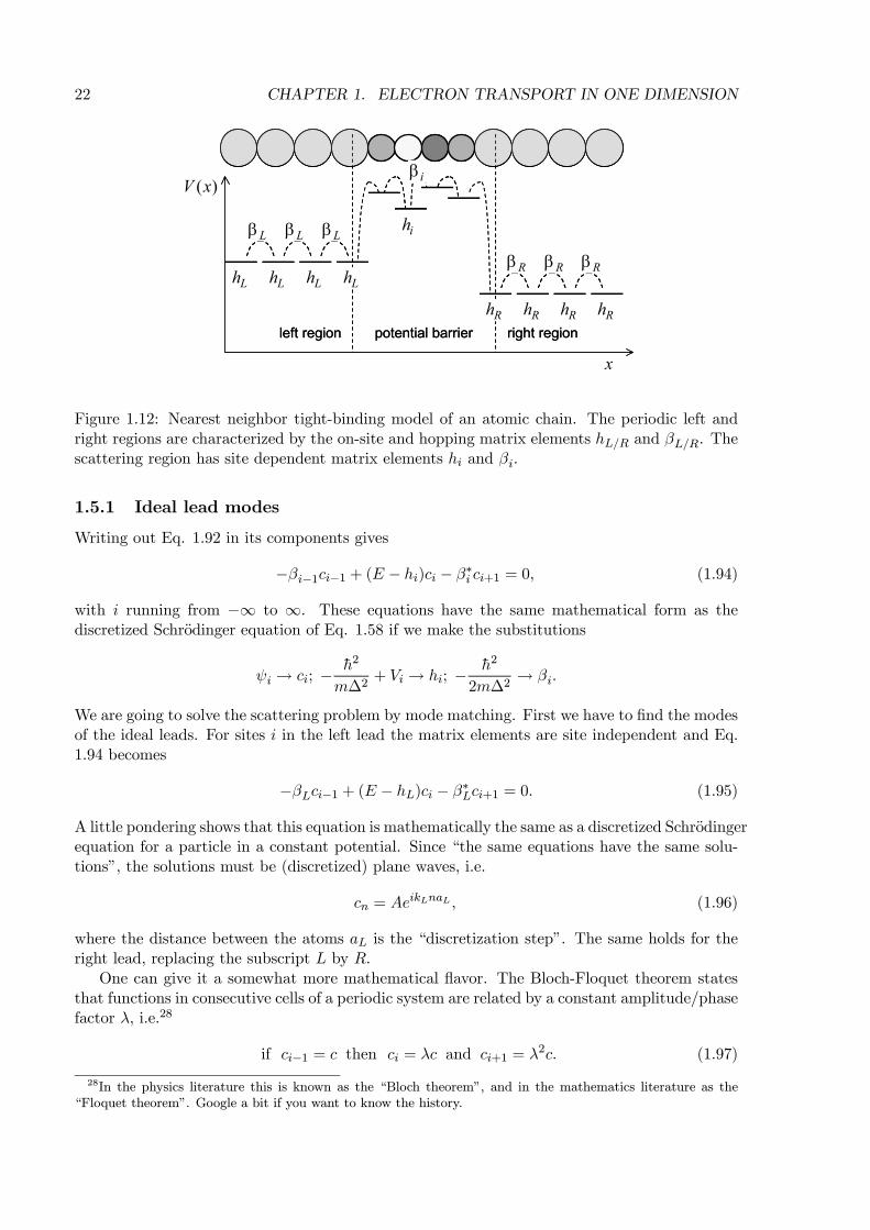
The model is called the nearest neighbor tight-binding approximation by physicists and amongchemists it is known as the Huckel approximation. The approximation is not essential and theformalism that I will explain below can be made to work for any LCAO representation, but hereI want to keep the expressions as simple as possible.27
We divide our system into three parts: a left lead, a scattering region, and a right lead. Theleft and right leads are perfect materials. They consist of identical atoms at equal distancesaL (for the left lead) and aR (for the right lead). In other words, the leads have translationalsymmetry. Matrix elements in the leads must be identical, i.e. hi = hL/R and βi = βL/R for theleft/right leads. Only in the scattering region do we have site dependent matrix elements. Thebasic idea is illustrated in Fig. 1.12.
26I want to keep things as simple as possible, so I am using an orthogal basis. If the atomic orbital basis isnon-orthogonal, then introduce an overlap matrix S, with matrix elements Si,j = hχi|χji, and substitute I by S.27In one-dimensional tight-binding one can assume that the hopping parameters βi are real, without loss of
generality. However, in three dimensions or in magnetic fields this need no longer be true. Therefore, to beprepared for the more general case, I keep complex βi’s for the moment.
22 CHAPTER 1. ELECTRON TRANSPORT IN ONE DIMENSION
( )V x
x
left region right regionpotential barrier
Lh Lh Lh Lh
Rh Rh Rh Rh
ihLβ Lβ Lβ
Rβ Rβ Rβ
iβ( )V x
x
left region right regionpotential barrier
Lh Lh Lh Lh
Rh Rh Rh Rh
ihLβ Lβ Lβ
Rβ Rβ Rβ
iβ
Figure 1.12: Nearest neighbor tight-binding model of an atomic chain. The periodic left andright regions are characterized by the on-site and hopping matrix elements hL/R and βL/R. Thescattering region has site dependent matrix elements hi and βi.
1.5.1 Ideal lead modes
Writing out Eq. 1.92 in its components gives
−βi−1ci−1 + (E − hi)ci − β∗i ci+1 = 0, (1.94)
with i running from −∞ to ∞. These equations have the same mathematical form as thediscretized Schrodinger equation of Eq. 1.58 if we make the substitutions
ψi → ci; − h2
m∆2+ Vi → hi; − h2
2m∆2→ βi.
We are going to solve the scattering problem by mode matching. First we have to find the modesof the ideal leads. For sites i in the left lead the matrix elements are site independent and Eq.1.94 becomes
−βLci−1 + (E − hL)ci − β∗Lci+1 = 0. (1.95)
A little pondering shows that this equation is mathematically the same as a discretized Schrodingerequation for a particle in a constant potential. Since “the same equations have the same solu-tions”, the solutions must be (discretized) plane waves, i.e.
cn = AeikLnaL , (1.96)
where the distance between the atoms aL is the “discretization step”. The same holds for theright lead, replacing the subscript L by R.
One can give it a somewhat more mathematical flavor. The Bloch-Floquet theorem statesthat functions in consecutive cells of a periodic system are related by a constant amplitude/phasefactor λ, i.e.28
if ci−1 = c then ci = λc and ci+1 = λ2c. (1.97)
28In the physics literature this is known as the “Bloch theorem”, and in the mathematics literature as the“Floquet theorem”. Google a bit if you want to know the history.
1.5. TIGHT-BINDING 23
Now is the time where we simplifying things a little bit by choosing β real,29 so Eq. 1.95 becomes
−β + (E − h)λ− βλ2 = 0⇒ (1.98)
λ =E − h2β
±"µE − h2β
¶2− 1# 12
,
where you can add the subscript L/R for the left and right leads. The roots λ can be given a
more familiar form. For¯E−h2β
¯≤ 1 we define a wave number k by30
cos(ka) =E − h2β
, (1.99)
which leads to the simple form
λ± = e±ika. (1.100)
λ± is called the Bloch factor. Using Eq. 1.97 recursively, i.e. cn = λnc0, then leads to Eq.1.96, with A = c0, as expected. It describes propagating waves, where λ+ describes a wavepropagating to the right, and λ− a wave propagating to the left.
For¯E−h2β
¯> 1 one can define κ by
cosh(κa) =
¯E − h2β
¯, (1.101)
and obtain
λ± = +e∓κa ifE − h2β
> 1;
λ± = −e∓κa ifE − h2β
< −1. (1.102)
Both these cases describe states that decay either to the right or to the left. These are calledevanescent states. They are not acceptable as solutions to the one-dimensional Schrodingerequation because one cannot normalize them (not even in the wave packet sense). However, wewill have a use for them later on in three-dimensional problems.
1.5.2 Mode matching
We have the modes of the ideal leads, so we can match them to the scattering region, where thematrix elements hi and βi in Eq. 1.94 are site dependent. We assume that the scattering regionis localized in space, so i runs from 1 to N . The procedure we have used to solve the discretizedSchrodinger problem in Sec. 1.4 can be copied with only some small modifications. Using Eq.1.100, Eqs. 1.61 and 1.64 read
c−1 = Aλ−1L,+ +Bλ−1L,− = Aλ
−1L,+ + (c0 −A)λ−1L,−; (1.103)
cN+2 = cN+1λR,+.
29which is always possible in one-dimensional systems, provided one has spin degeneracy and time-inversionsymmetry, which we have here.30You may recognize E(k) = h+2β cos ka as the dispersion relation describing an electronic band in the nearest
neighbor tight-binding model.
24 CHAPTER 1. ELECTRON TRANSPORT IN ONE DIMENSION
The convention is to write ci+n = λnci, where n is an integer (positive or negative), and let the± indicate waves propagating to the left and right, respectively.31 These relations can be usedto substitute Eq. 1.92 by ¡
EI−H0¢ψ = q, (1.104)
similar to Eq. 1.66. ψ is a finite dimensional vector that contains the coefficients ci in thescattering region plus those of the two boundaries, i.e. i = 0, . . . ,N + 1. q is the “source”vector of length N + 2, whose coefficients are zero, except the first one
q0 = βLAnλ−1L,− − λ−1L,+
o. (1.105)
H0 is a finite (N+2)× (N+2) Hamiltonian matrix. All its matrix elements are identical to thatof the original Hamiltonian matrix, Eq. 1.93, except for the first and the last diagonal element,which are modified to
H 00,0 = h0 +ΣL(E);
H 0N+1,N+1 = hN+1 +ΣR(E), (1.106)
with
ΣL(E) = βLλ−1L,−;
ΣR(E) = βRλR,+. (1.107)
These self-energies contain all the information concerning the coupling of the scattering regionto the leads. As before, they are complex and energy dependent through Eqs. 1.99 and 1.100.
We have substituted an infinite dimensional problem, Eq. 1.92, by a finite dimensional one,Eq. 1.104!! 32 Mathematically Eq. 1.104 is the same as Eq. 1.66. Again “the same equationshave the same solutions”, so according to Eq. 1.72, the transmission amplitude becomes
t =
rvRvL
cN+1A
(1.108)
with, as in Eq. 1.77, the velocities given by
vL/R = −2aL/Rh
ImΣL/R(E). (1.109)
In addition, the Green function expressions given in Sec. 1.4.1 remain valid.
31In the one-dimensional case, one always has λ+ = 1/λ−. In the three-dimensional case, this relation does notnecessarily hold. That’s why it is important to keep separate track of the powers of λ and the ± indices.32For those of you who have some background in this, you might suspect that the technique we are using here
has something to do with a technique known as partitioning. This suspicion is appropriate. Partitioning isusually applied to operators and, in particular, to Green functions. I am applying it to wave functions here.
Chapter 2
Electron transport in threedimensions
In this chapter I want to upgrade the discussion of the previous chapter to problems in three di-mensions. The tunnel junction of Fig. 1.2, for instance, is clearly not a strictly one-dimensionaldevice. In Sec. 2.1 we will generalize Landauer’s formula for the conductance to three dimen-sions. I will do this in steps of increasing complexity, i.e. start with plane waves and squarebarriers, as in the one-dimensional (1D) case, and end with atomistic three-dimensional (3D)devices. The techniques that are introduced should allow us to study transport at the nanoscalein any small system. In a tunnel junction the dimension of the device across the junction (de-termined by the thickness of the insulator layer) is usually much smaller that the dimensionsparallel to the metal insulator interfaces. The modeling then becomes easier if one assumes thelatter dimensions to be infinite and one uses translation symmetry along the interfaces. Thelatter requires doing a bit of solid state physics. Another “device” is shown in Fig. 2.8 below. Itconsists of a mono-atomic wire sandwiched between two electrodes. Such wires have been madeof gold atoms, for instance. Clearly the wire is finite in all three dimensions and the electrodesare infinite. Our modeling must be able to cope both with finite and with infinite dimensions.
As in the previous chapter, Landauer’s formula expresses the conductance in terms of thetransmission of incoming electron waves. In three dimensions the transmission amplitudes con-stitute a matrix, the transmission matrix, whose calculation is our primary task. Practicalalgorithms are explained in Sec. 2.2. In particular, the mode matching techniques of Sec. 1.4are generalized to 3D. Since in 3D the derivations of the expressions become quite lengthy andtechnical, I won’t give all details. They can be found in the literature.
2.1 Landauer in 3D
2.1.1 Conductance of model interfaces
We start with a generalization of the square barrier potential of Fig. 1.3. A two-dimensionalexample is shown in Fig. 2.1. The potential V (x, y) is separable; the barrier is in the x-directionand the potential is independent of y. The straightforward extension to three dimensions is apotential that is independent of y and z. Such a potential landscape is a simple model for a thinlayer of an insulator sandwiched between two metals, i.e. a tunnel junction.
The Schrodinger equation
Eψ(r) +h2
2m∇2ψ(r)− V (r)ψ(r) = 0 (2.1)
25

26 CHAPTER 2. ELECTRON TRANSPORT IN THREE DIMENSIONS
iAe ⋅k r
iBe ⋅- k r
iFe ⋅k r
(V x, y)
x
left region right regionmiddle regiony
iAe ⋅k r
iBe ⋅- k r
iFe ⋅k r
(V x, y)
x
left region right regionmiddle regiony
Figure 2.1: A square barrier in two dimensions. In the left and right regions the potential isconstant, V (x, y) = V1. In the middle region the potential is also constant, V (x, y) = V0, whereV0 > V1. The incoming, reflected and transmitted waves are given by Ae
ik·r, Beik0·r and Feik·r,see Fig. 2.2.
is separable in Cartesian coordinates·E +
½h2
2m
d2
dx2− V (x)
¾+h2
2m
d2
dy2+h2
2m
d2
dz2
¸ψ(x, y, z) = 0,
and its solutions can be written as
ψ(x, y, z) = φ(x)eikyyeikzz = φ(x)eikk·r; kk =
0kykz
, (2.2)
where eikk·r describes a free particle in the direction parallel to the barrier. The function φ(x)is the solution of the one-dimensional scattering problem·
Ex +
½h2
2m
d2
dx2− V (x)
¾¸φ(x) = 0, (2.3)
with the energy
Ex = E −h2k2k2m
.. (2.4)
Note that kk is a good quantum number1, which together with the energy E fixes the wavefunction. We say that kk defines a mode of the system.
A view of the scattering geometry in the¡kx,kk
¢plane is given in Fig. 2.2. In the left and
right regions the wave function is
ψkk(r) =
Aheik·r + rkk(E)e
ik0·ri; r in left region
Ahtkk(E)e
ik·ri; r in right region
(2.5)
1a set of two quantum numbers, actually.
2.1. LANDAUER IN 3D 27
left region right regionmiddle regionk
k'k
k ||
k || k ||
xk
xk− xkleft region right regionmiddle region
k
k'k
k ||k ||
k ||k || k ||k ||
xk
xk− xk
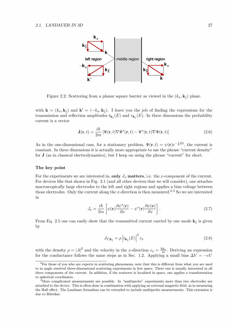
Figure 2.2: Scattering from a planar square barrier as viewed in the (kx,kk) plane.
with k = (kx,kk) and k0 = (−kx,kk). I leave you the job of finding the expressions for thetransmission and reflection amplitudes tkk(E) and rkk(E). In three dimensions the probabilitycurrent is a vector
J(r, t) =ih
2m[Ψ(r, t)∇Ψ∗(r, t)−Ψ∗(r, t)∇Ψ(r, t)] (2.6)
As in the one-dimensional case, for a stationary problem, Ψ(r, t) = ψ(r)e−ihEt, the current is
constant. In three dimensions it is actually more appropriate to use the phrase “current density”for J (as in classical electrodynamics), but I keep on using the phrase “current” for short.
The key point
For the experiments we are interested in, only Jx matters, i.e. the x-component of the current.For devices like that shown in Fig. 2.1 (and all other devices that we will consider), one attachesmacroscopically large electrodes to the left and right regions and applies a bias voltage betweenthose electrodes. Only the current along the x-direction is then measured.2,3 So we are interestedin
Jx =ih
2m
·ψ(r)
∂ψ∗(r)∂x
− ψ∗(r)∂ψ(r)
∂x
¸. (2.7)
From Eq. 2.5 one can easily show that the transmitted current carried by one mode kk is givenby
JT,kk = ρ¯tkk(E)
¯2vx (2.8)
with the density ρ = |A|2 and the velocity in the x-direction vx = hkxm . Deriving an expression
for the conductance follows the same steps as in Sec. 1.2. Applying a small bias ∆V = −eU2For those of you who are experts in scattering phenomena, note that this is different from what you are used
to in angle resolved three-dimensional scattering experiments in free space. There one is usually interested in allthree components of the current. In addition, if the scatterer is localized in space, one applies a transformationto spherical coordinates.
3More complicated measurements are possible. In “multiprobe” experiments more than two electrodes areattached to the device. This is often done in combination with applying an external magnetic field, as in measuringthe Hall effect. The Landauer formalism can be extended to include multiprobe measurements. This extension isdue to Buttiker.
28 CHAPTER 2. ELECTRON TRANSPORT IN THREE DIMENSIONS
between left and right regions, the transmitted current is carried by all modes that have anenergy Ek in the range from EF −∆V to EF , see Fig. 1.7.
JT = 2ρX
EF−∆V <Ek<EF
¯tkk(E)
¯2vx, (2.9)
where the factor 2 accounts for the degeneracy. We can use the same tricks as in Sec. 1.2.Using states that are normalized in a 3D, we have ρ = 1
2L3; compare to Eq. 1.32.4 We writeP
EF−∆V <Ek<EF =Pkk
Pkx, where one has to sum only over those states that have their
energy in the indicated interval. ConvertPkxinto a one-dimensional integral, use vx =
1hdExdkx,
and assume that tkk(E) is independent of the energy in the small energy range ∆V . The algebrais
JT =1
L3
Xkk
Xkx
¯tkk(E)
¯2vx =
1
L3
Xkk
L
π
Z ¯tkk(E)
¯2vxdkx
=1
L21
π
Xkk
Z ¯tkk(E)
¯2 1h
dExdkx
dkx =1
L21
πh
Xkk
Z EF−h2k2k2m
EF−∆V−h2k2k2m
¯¯tkk(Ex + h
2k2k2m
)
¯¯2
dEx
=1
L2∆V
πh
Xkk
¯tkk(EF )
¯2. (2.10)
The transmitted current is IT =RJT · dS = JTL2 and the conductance G = IT/U is then given
by
G = e2
πh
Xkk
¯tkk(EF )
¯2=e2
πhT (EF ). (2.11)
The expression is the Landauer formula, see Eq. 1.29, with the total transmission T expressedas a sum over the transmissions of the individual modes kk. One has to sum over the kk thatcontribute to the transmission at the Fermi energy EF .
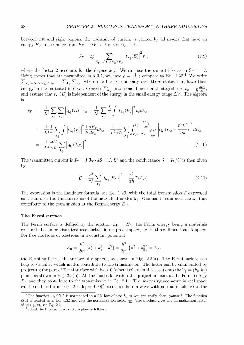
The Fermi surface
The Fermi surface is defined by the relation Ek = EF , the Fermi energy being a materialsconstant. It can be visualized as a surface in reciprocal space, i.e. in three-dimensional k-space.For free electrons or electrons in a constant potential
Ek =h2
2m
¡k2x + k
2y + k
2z
¢=h2
2m
³k2x + k
2k´= EF .
the Fermi surface is the surface of a sphere, as shown in Fig. 2.3(a). The Fermi surface canhelp to visualize which modes contribute to the transmission. The latter can be enumerated byprojecting the part of Fermi surface with kx > 0 (a hemisphere in this case) onto the kk = (ky, kz)plane, as shown in Fig. 2.3(b). All the modes kk within this projection exist at the Fermi energyEF and they contribute to the transmission in Eq. 2.11. The scattering geometry in real spacecan be deduced from Fig. 2.2. kk = (0, 0)5 corresponds to a wave with normal incidence to the
4The function 1L2eikk·r is normalized in a 2D box of size L, as you can easily check yourself. The function
φ(x) is treated as in Eq. 1.32 and gets the normalization factor 12L. The product gives the normalization factor
of ψ(x, y, z), see Eq. 2.2.5called the Γ-point in solid state physics folklore.
2.1. LANDAUER IN 3D 29
xk
yk
zk= FE Ek
yk
zk
yk
zk
(a) (b) (c)xk
yk
zk
yk
zk= FE Ek
yk
zk
yk
zk
yk
zk
yk
zk
yk
zk
(a) (b) (c)
Figure 2.3: (a) The Fermi surface, as defined by Ek = EF , of electrons in a constant potentialis a sphere. (b) The projection of the surface in the kk = (ky, kz) plane. The shaded area
denotes all the kk modes that contribute to the transmission at EF . (c) The transmission¯tkk
¯2as function of kk. Red indicates a high transmission and blue a low transmission. The highesttransmission is for kk = (0, 0). It decreases to 0 towards the edge of the circle.
barrier. The larger kk =¯kk¯, the more glancing the incidence of the corresponding wave. At
the edge of the circle in Fig. 2.3(b) one has h2
2mk2k = EF , so kx = 0, and the corresponding wave
propagates parallel to the barrier.For a simple square barrier one can easily calculate the transmission. If the Fermi energy is
less than the barrier height, the transmission of a single mode is given by¯tkk(EF )
¯2= T1D(Ex) = T1D(EF −
h2k2k2m
), (2.12)
with T1D given by Eqs. 1.47 and 1.42. The result is visualized in Fig. 2.3(c). Since T1D is amonotonically increasing function of the energy, the maximal transmission is for kk = (0, 0), i.e.for normal incidence. The transmission decreases monotonically with increasing kk, i.e. withthe angle of incidence, until it is zero for parallel incidence. Such a simple Fermi surface and asimple transmission are typical for free electrons. For real materials both the Fermi surface andthe transmission are much more complex. I will come back to in Sec. 2.1.4.
2.1.2 Conductance of model wires: the ballistic conductance
The way we have derived Eq. 2.11 means it can easily be generalized to any system whoseHamiltonian is separable in an x-term and a yz-term. For instance, the wave functions of thewire shown in Fig. 2.4 can be written as
ψ(x, r⊥) = φ(x)ηn(r⊥), (2.13)
where n is a set of two quantum numbers labeling the modes; see Eq. 2.2. The conductance ofthis quantum wire can be expressed as the sum of the transmissions of the individual modes
G = e2
πh
Xn
|tn(EF )|2 . (2.14)
Suppose we are dealing with an ideal wire in which all the modes are fully transmitted.6
6which is the definition of an ideal wire.
30 CHAPTER 2. ELECTRON TRANSPORT IN THREE DIMENSIONS
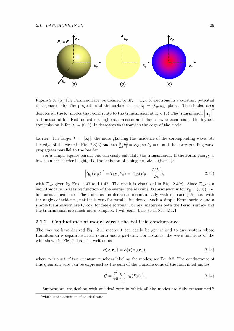
x
r⊥
x
r⊥r⊥
Figure 2.4: A simple (quantum) wire.
The transmission is maximal, i.e. |tn(EF )|2 = 1 for each mode n, and the conductance is
Gbal = e2
πhM(EF ), (2.15)
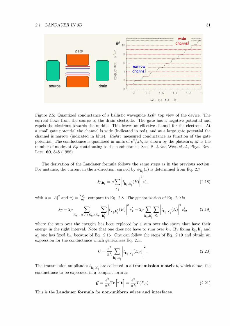
where M(EF ) is the number of modes at the Fermi energy, supported by the wire. Gbal is calledthe ballistic conductance. The number of modes at fixed energy in a wire of finite crosssection is finite. So even for a perfect wire the conductance is finite!! If the cross section ismacroscopically large, the number of modes is very large. Measuring the ballistic conductanceexperimentally is then impossible. A real wire always contains impurities and imperfections (lat-tice defects, grain boundaries, impurity atoms, etc.), and scattering at these defects dominatesthe conductance. However, thin and small wires can be made without any defects. Note that,since the number of modes is an integer, the conductance of Eq. 2.15 is quantized.
A very clear example of quantized conductance is presented by the experiment of van Weeset al. on the quantum conductance of a channel in a two-dimensional electron gas (2DEG). A2DEG is formed at an interface between two well-chosen semiconductors. Putting electrodes ontop of the 2DEG it is possible do define a one-dimensional channel (the “wire”) by a suitableelectrostatic potential profile, as illustrated in Fig. 2.5. The width of the channel determinesthe number of modes at the Fermi energyM(EF ). Upon widening the channel, which is done bymaking the gate less repulsive for electrons, the number of modes increases and the conductanceincreases. However, it increases in steps of e
2
πh . This is demonstrated by the experimental results,shown in Fig. 2.5.
2.1.3 Conductance of combined interfaces and wires
In the real world interfaces nor wires are infinite. This leads to Hamiltonians that are notseparable in an x-term and a yz-term. A two-dimensional example is shown in Fig. 2.6, whichrepresents a canyon through a 2D square barrier. It is a simple model for a finite wire connectedto two electrodes (the left and right regions). An incoming wave Aeik·r with k = (kx,kk) can bescattered into any other wave Ceik
0·r with k0 = (k0x,k0k) provided the energy is conserved, i.e.
h2(k2x + k2k)
2m= E =
h2(k02x + k02k )
2m. (2.16)
The idea is shown in Fig. 2.7. The wave function of Eq. 2.5 is generalized to
ψkk(r) =
A
·eik·r +
Pk00krkk,k
00k(E)eik
00 ·r¸; r in left region
A
·Pk0ktkk,k
0k(E)eik
0·r¸; r in right region
(2.17)
where k0 labels the transmitted waves, i.e. k0x > 0, and k00 labels the reflected waves, i.e. k00x < 0,
all at the same energy. The reflection and transmission amplitudes rkk,k00kand t
kk,k0kindicate
the probability amplitudes of scattering from a mode kk to a mode k00k or k
0k.
2.1. LANDAUER IN 3D 31
Figure 2.5: Quantized conductance of a ballistic waveguide Left: top view of the device. Thecurrent flows from the source to the drain electrode. The gate has a negative potential andrepels the electrons towards the middle. This leaves an effective channel for the electrons. Ata small gate potential the channel is wide (indicated in red), and at a large gate potential thechannel is narrow (indicated in blue). Right: measured conductance as function of the gatepotential. The conductance is quantized in units of e2/πh, as shown by the plateau’s; M is thenumber of modes at EF contributing to the conductance. See: B. J. van Wees et al., Phys. Rev.Lett. 60, 848 (1988).
The derivation of the Landauer formula follows the same steps as in the previous section.For instance, the current in the x-direction, carried by ψkk(r) is determined from Eq. 2.7
JT,kk = ρXk0k
¯tkk,k
0k(E)
¯2v0x, (2.18)
with ρ = |A|2 and v0x = hk0xm ; compare to Eq. 2.8. The generalization of Eq. 2.9 is
JT = 2ρX
EF−∆V <Ek<EF
Xk0k
¯tkk,k
0k(E)
¯2v0x = 2ρ
Xkk,k
0k
Xk0x
¯tkk,k
0k(E)
¯2v0x, (2.19)
where the sum over the energies has been replaced by a sum over the states that have theirenergy in the right interval. Note that one does not have to sum over kx. By fixing kk,k
0k and
k0x one has fixed kx, because of Eq. 2.16. One can follow the steps of Eq. 2.10 and obtain anexpression for the conductance which generalizes Eq. 2.11
G = e2
πh
Xkk,k
0k
¯tkk,k
0k(EF )
¯2. (2.20)
The transmission amplitudes tkk,k0kare collected in a transmission matrix t, which allows the
conductance to be expressed in a compact form as
G = e2
πhTrht†ti=e2
πhT (EF ). (2.21)
This is the Landauer formula for non-uniform wires and interfaces.
32 CHAPTER 2. ELECTRON TRANSPORT IN THREE DIMENSIONS
iAe ⋅k r
iBe ⋅''k r
iFe ⋅'k r
(V x, y)
x
left region right regionmiddle regiony
iAe ⋅k r
iBe ⋅''k r
iFe ⋅'k r
(V x, y)
x
left region right regionmiddle regiony
Figure 2.6: A simple model for a wire connected to two electrodes (the left and right regions)as a canyon through a square barrier. The incoming wave Aeik·r can be reflected to any waveBeik
00·r or transmitted to any wave Feik0·r, provided the energy is conserved.
left region
right regionmiddle region
k
'k
"k
k ||
"k ||
'k ||
xk
"xk
'xkleft region
right regionmiddle region
k
'k
"k
k ||k ||
"k ||
'k ||
xk
"xk
'xk
Figure 2.7: Scattering from a finite wire between two electrodes as viewed in the¡kx,kk
¢plane.
Only one of the possible reflected³k00x,k00k
´waves and one of the transmitted
³k0x,k0k
´waves are
indicated.
2.1.4 Conductance of atomistic wires and interfaces
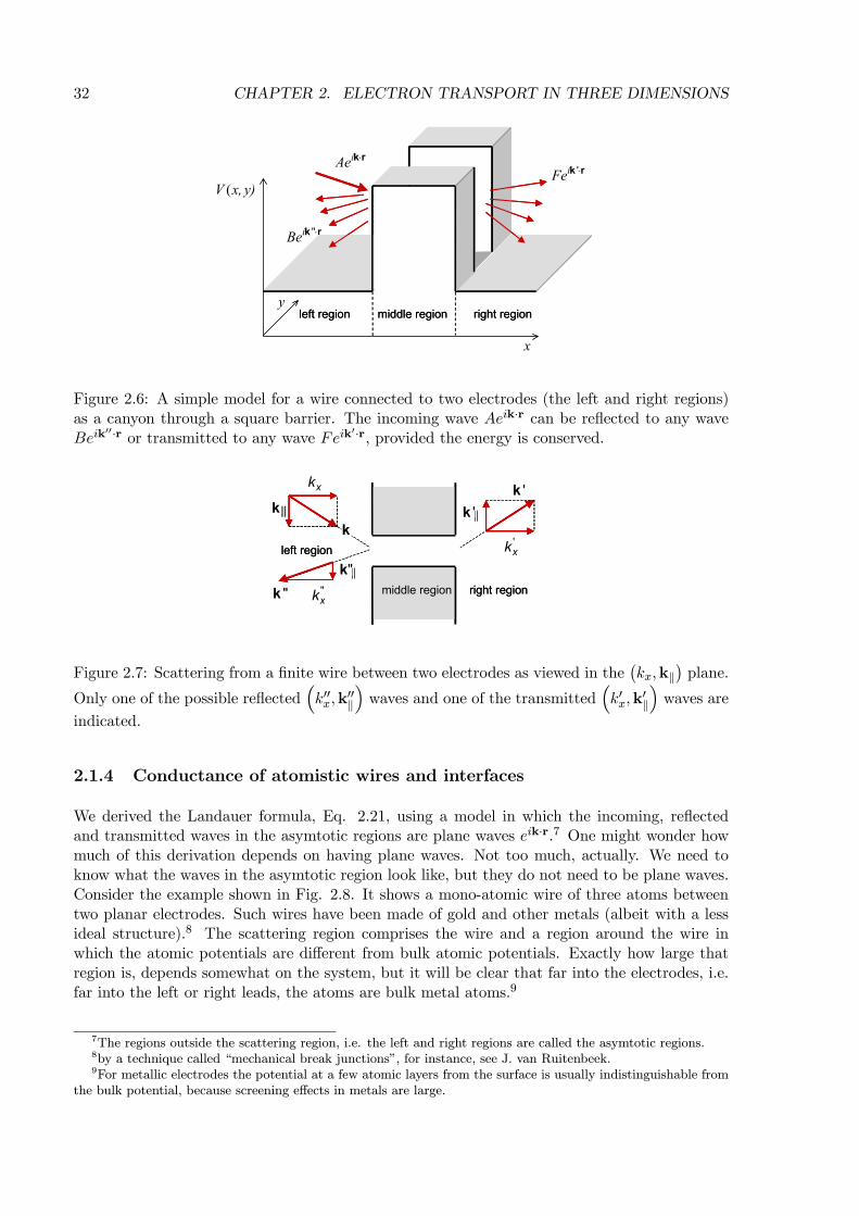
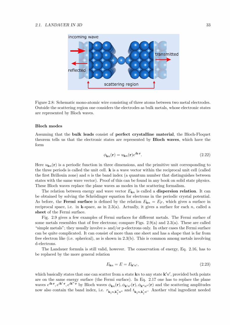
We derived the Landauer formula, Eq. 2.21, using a model in which the incoming, reflectedand transmitted waves in the asymtotic regions are plane waves eik·r.7 One might wonder howmuch of this derivation depends on having plane waves. Not too much, actually. We need toknow what the waves in the asymtotic region look like, but they do not need to be plane waves.Consider the example shown in Fig. 2.8. It shows a mono-atomic wire of three atoms betweentwo planar electrodes. Such wires have been made of gold and other metals (albeit with a lessideal structure).8 The scattering region comprises the wire and a region around the wire inwhich the atomic potentials are different from bulk atomic potentials. Exactly how large thatregion is, depends somewhat on the system, but it will be clear that far into the electrodes, i.e.far into the left or right leads, the atoms are bulk metal atoms.9
7The regions outside the scattering region, i.e. the left and right regions are called the asymtotic regions.8by a technique called “mechanical break junctions”, for instance, see J. van Ruitenbeek.9For metallic electrodes the potential at a few atomic layers from the surface is usually indistinguishable from
the bulk potential, because screening effects in metals are large.
2.1. LANDAUER IN 3D 33
Figure 2.8: Schematic mono-atomic wire consisting of three atoms between two metal electrodes.Outside the scattering region one considers the electrodes as bulk metals, whose electronic statesare represented by Bloch waves.
Bloch modes
Assuming that the bulk leads consist of perfect crystalline material, the Bloch-Floquettheorem tells us that the electronic states are represented by Bloch waves, which have theform
φkn(r) = ukn(r)eik·r. (2.22)
Here ukn(r) is a periodic function in three dimensions, and the primitive unit corresponding tothe three periods is called the unit cell. k is a wave vector within the reciprocal unit cell (calledthe first Brillouin zone) and n is the band index (a quantum number that distinguishes betweenstates with the same wave vector). Proof of this can be found in any book on solid state physics.These Bloch waves replace the plane waves as modes in the scattering formalism.
The relation between energy and wave vector Ekn is called a dispersion relation. It canbe obtained by solving the Schrodinger equation for electrons in the periodic crystal potential.As before, the Fermi surface is defined by the relation Ekn = EF , which gives a surface inreciprocal space, i.e. in k-space, as in 2.3(a). Actually, it gives a surface for each n, called asheet of the Fermi surface.
Fig. 2.9 gives a few examples of Fermi surfaces for different metals. The Fermi surface ofsome metals resembles that of free electrons; compare Figs. 2.9(a) and 2.3(a). These are called“simple metals”; they usually involve s- and/or p-electrons only. In other cases the Fermi surfacecan be quite complicated. It can consist of more than one sheet and has a shape that is far fromfree electron like (i.e. spherical), as is shown in 2.3(b). This is common among metals involvingd-electrons.
The Landauer formula is still valid, however. The conservation of energy, Eq. 2.16, has tobe replaced by the more general relation
Ekn = E = Ek0n0 , (2.23)
which basically states that one can scatter from a state kn to any state k0n0, provided both pointsare on the same energy surface (the Fermi surface). In Eq. 2.17 one has to replace the planewaves eik·r, eik0·r, eik00·r by Bloch waves φkn(r),φk0n0(r),φk00n00(r) and the scattering amplitudesnow also contain the band index, i.e. rkkn,k
00k n
00 and tkkn,k0kn
0 . Another vital ingredient needed

34 CHAPTER 2. ELECTRON TRANSPORT IN THREE DIMENSIONS
xk
yk
zk
=1 FE Ek
(a) (b)
=1 FE Ek =2 FE Ek =3 FE Ek
xk
yk
zk
=1 FE Ek
(a) (b)
=1 FE Ek =2 FE Ek =3 FE Ek
Figure 2.9: (a) The Fermi surface of Cu (copper). The wireframe indicates the first Brillouinzone (the reciprocal unit cell). The Fermi surface is almost spherical with a few holes punchedthrough it. In Cu there is only one s-like band crossing the Fermi energy, which gives rise toone sheet. (b) The Fermi surface of fcc Co (Cobalt) for the minority spin electrons. Co is aferromagnetic material. Only one s-like majority spin band crosses the Fermi energy, whichgives rise to a Fermi surface for majority spin electrons that resembles that of Cu. Three d-likeminority spin bands cross the Fermi energy, giving rise to three sheets of the Fermi surface thatare far from spherical, as is shown here.
is an expression for the velocity v0x. In solid state textbooks it is shown that the Bloch velocityis given by
v0x =1
h
∂Ek0n0
∂k0x. (2.24)
A little pondering shows that this is just the relation we need to complete the derivation of theLandauer formula.
G = e2
πh
Xkkn,k
0kn
0
¯tkkn,k
0kn
0(EF )
¯2=e2
πhTrht†ti. (2.25)
An example: the conductance of an interface between copper and cobalt
Does it matter whether one takes real metals with Bloch modes as electrodes, or jellium metals,where the modes are plane waves? As an example that it does matter I will discuss the con-ductance of a simple interface between the metals copper (Cu) and cobalt (Co). Bulk Cu hasa fcc (face centered cubic) close packed structure. Its (111) surface is close packed and it formsthe crystal termination with the lowest surface energy. Bulk Co has the hcp (hexagonally closepacked) structure. However if one deposits a thin layer of Co on Cu(111), then Co assumes afcc structure with the lattice parameter of Cu. So the (111) interface between Cu and Co hasa simple structure. So far we have considered spin degenerate systems, i.e. spin-up electronsare described by the same wave functions as spin-down electrons. This hold for Cu, which is anon-magnetic material. It does not hold for Co, which is a magnetic material, and both spinshave different wave functions. In addition the number of spin-up electrons is not equal to thenumber of spin-down electrons (which is why the material is magnetic). The obvious namesmajority spin and minority spin are used.

2.1. LANDAUER IN 3D 35
The Landauer formula can be generalized to include the spin states explicitly in a straight-forward manner
G = e2
2πh
Xkknσ,k
0kn
0σ0
¯tkknσ,k
0kn
0σ0(EF )
¯2, (2.26)
where σ,σ0 = −12 , 12 . In absence of spin-orbit coupling the scattering potential does not flip thespin and the transmission matrix is diagonal in the spin t
kknσ,k0kn
0σ0 = tkknσ,k0kn
0σδσσ0 . This is
accurate for (magnetic) 3d transition metals and lighter elements.One can use the same procedure as in Fig. 2.3 to visualize the transmission. The Fermi
surfaces of Cu and of the minority spin of Co are given in Fig. 2.9. The Fermi surface of themajority spin of Co resembles that of Cu. One has to project these surfaces onto the kk plane,i.e. along the transport direction, which is the (111) direction in this case. In Fig. 2.9(a) (111)is the direction pointing from the origin to the center of a hexagon. The projection of the Fermisurface of Cu is shown in Fig. 2.10(a). The projected Fermi surface for the majority spin of Cois shown in Fig. 2.10(b). As stated, it is quite similar to that of Cu. The Fermi surface for theminority spin of Co is much more complicated, as shown in Fig. 2.9 (b). Projecting all threesheets in the (111) direction on top of one another gives the result shown in Fig. 2.10(c).
For a perfect crystalline interface kk is a good quantum number and the transmission matrixis diagonal in kk (as well as in σ) t
kknσ,k0kn
0σ0 = tkknσ,kkn0σδkkk0kδσσ0 . For the majority spin¯
tkk1σ,kk1σ
¯2describes the transmission from the state kk1σ on the projected Fermi surface of
Cu (indicated by a black dot in Fig. 2.10(a)) to a state kk1σ on the projected majority spinFermi surface of Co (indicated by a black dot in Fig. 2.10(b)).10 The calculated transmission¯tkk1σ,kk1σ
¯2is shown in Fig. 2.10(d) in the kk plane. The transmission is a number between
0 and 1. Obviously the state kk1σ has to exist on the Cu Fermi surface; otherwise one has noelectrons to start with. Around kk = (0, 0) the Cu Fermi surface has a “hole” where there areno states, which is indicated in white in 2.10(a) and (d). Then the state kk1σ has to exist on theCo Fermi surface; otherwise there is no state to transport the electrons to and the transmissionis 0. These are the blue area’s in Fig. 2.10(d). The remaining area is almost entirely red, whichmeans that there the transmission is close to 1.
Fig. 2.10(e) shows the calculated transmissionP3n0=1
¯tkk1σ,kkn0σ
¯2between the minority spin
modes of Cu and Co. As one can observe, the transmission pattern is much more complicatedthan in the majority spin case with a fine-grained variation of the transmission between 0 and1. Now compare Figs. 2.10(d) and (e) to Fig. 2.3 (c). It represents the difference between usingreal metals and using jellium.11
Integrating over the area shown in Fig. 2.10(d) gives the majority spin conductance; the
calculated number is Gmaj = e2
2πh0.73. Integrating over the area shown in Fig. 2.10(e) gives
the minority spin conductance Gmin = e2
2πh0.66. The difference in the conductance between themajority and the minority spin modes is 10%. One can enlarge this difference by making amultilayer of alternating Cu and Co layers since such a multilayer then contains many Cu/Cointerfaces. The majority/minority difference in the conductance essentially gives the so-calledGMR (giant magneto-resistance) effect that is measured in such multilayers.12
10n = 1 and n0 = 1, since both Fermi surfaces have only one sheet.11Jellium also does not give magnetism at these electronic densities, but I don’t want to make a list of what’s
wrong with jellium.12The GMR effect is used to make sensitive sensors for magnetic fields, which are used in the heads of magnetic
hard drives. It contributed to the rapid development in hard disks to the >102 Gb disks we have today.

36 CHAPTER 2. ELECTRON TRANSPORT IN THREE DIMENSIONS
Figure 2.10: (a) Fermi surface of Cu projected in the (111) direction on the kk plane. (b) Fermisurface of the majority spin of Co projected on the same plane. (c) The three sheets of the Fermisurface of the minority spin of Co projected in the same plane. Blue, green and red indicatearea’s where 1,2 and 3 states are projected onto the same kk point. (d) The transmission acrossa (111) interface between the Cu and the majority spin in Co, as a function of kk. The colorscale indicates the transmission from 0 (blue) to 1 (red). (e) As (d), but for the transmissionbetween Cu and the minority spin of Co. The white area’s indicate where there are no states inCu.
2.2 Calculating the transmission
As will be clear by now, the key quantity for calculating the conductance is the transmissionmatrix t. This is quite a bit more complicated than in the one-dimensional case, but in principleall the techniques discussed in Secs. 1.4 and 1.5 can be extended to calculate transmissionmatrices in three dimensions for systems containing real atoms. Since the tight-binding examplegiven in Sec. 1.5 is chemically the most intuitive, I use this and focus upon the mode matchingtechnique.
The principal idea is to divide your system into layers of atoms, normal to the transportdirection. One chooses the layers to be sufficiently thick such that the Hamiltonian matrix onlycontains matrix elements that either couple atoms within one layer, or atoms that are in nearest
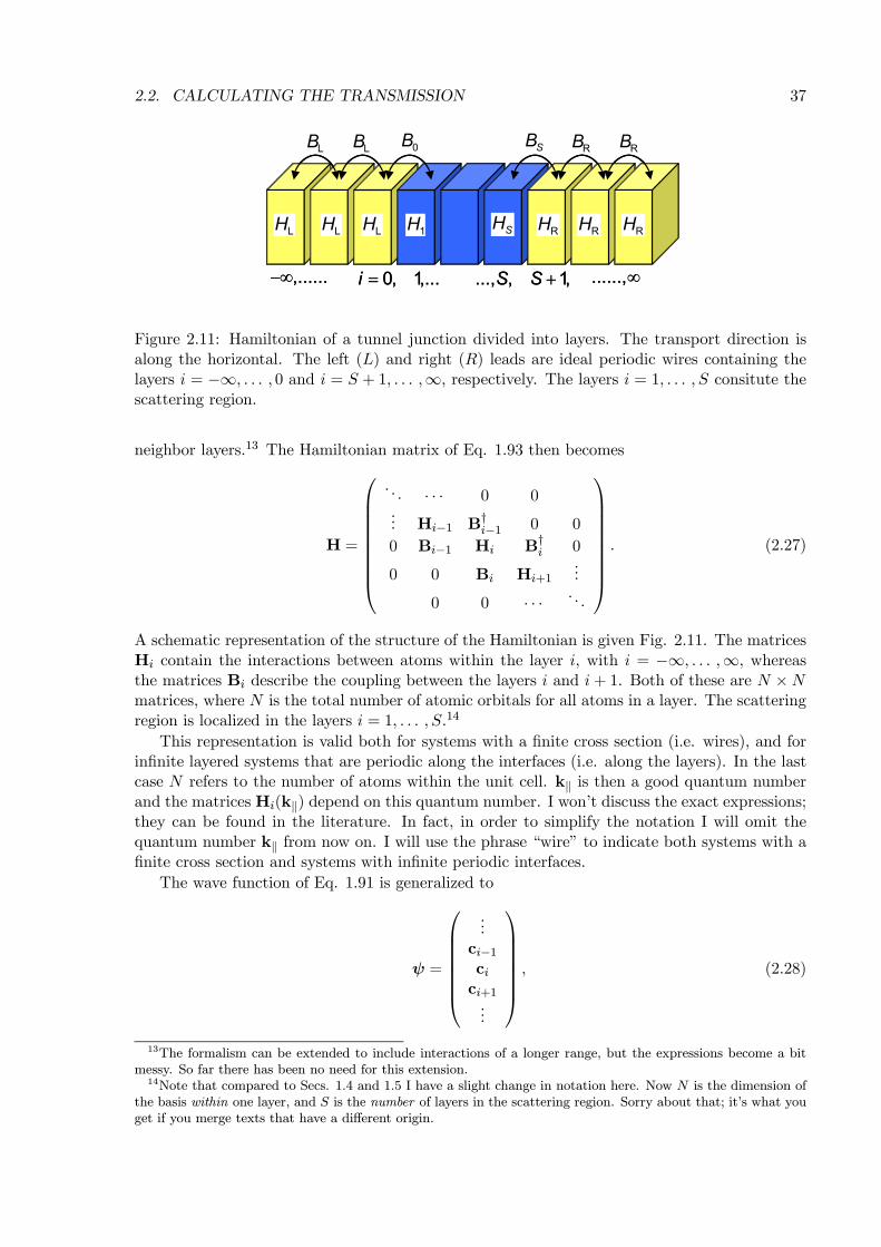
2.2. CALCULATING THE TRANSMISSION 37
......,∞,......−∞ 0, 1,...i = ..., , 1,S S +
LH LH LH RH RH RH1H SH
LB LB RB RB0B SB
......,∞,......−∞ 0, 1,...i = ..., , 1,S S +
LH LH LH RH RH RH1H SH
LB LB RB RB0B SB
Figure 2.11: Hamiltonian of a tunnel junction divided into layers. The transport direction isalong the horizontal. The left (L) and right (R) leads are ideal periodic wires containing thelayers i = −∞, . . . , 0 and i = S + 1, . . . ,∞, respectively. The layers i = 1, . . . , S consitute thescattering region.
neighbor layers.13 The Hamiltonian matrix of Eq. 1.93 then becomes
H =
. . . · · · 0 0... Hi−1 B†i−1 0 0
0 Bi−1 Hi B†i 0
0 0 Bi Hi+1...
0 0 · · · . . .
. (2.27)
A schematic representation of the structure of the Hamiltonian is given Fig. 2.11. The matricesHi contain the interactions between atoms within the layer i, with i = −∞, . . . ,∞, whereasthe matrices Bi describe the coupling between the layers i and i+ 1. Both of these are N ×Nmatrices, where N is the total number of atomic orbitals for all atoms in a layer. The scatteringregion is localized in the layers i = 1, . . . , S.14
This representation is valid both for systems with a finite cross section (i.e. wires), and forinfinite layered systems that are periodic along the interfaces (i.e. along the layers). In the lastcase N refers to the number of atoms within the unit cell. kk is then a good quantum numberand the matrices Hi(kk) depend on this quantum number. I won’t discuss the exact expressions;they can be found in the literature. In fact, in order to simplify the notation I will omit thequantum number kk from now on. I will use the phrase “wire” to indicate both systems with afinite cross section and systems with infinite periodic interfaces.
The wave function of Eq. 1.91 is generalized to
ψ =
...ci−1cici+1...
, (2.28)
13The formalism can be extended to include interactions of a longer range, but the expressions become a bitmessy. So far there has been no need for this extension.14Note that compared to Secs. 1.4 and 1.5 I have a slight change in notation here. Now N is the dimension of
the basis within one layer, and S is the number of layers in the scattering region. Sorry about that; it’s what youget if you merge texts that have a different origin.
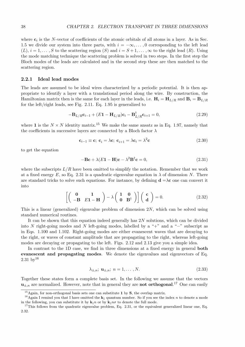
38 CHAPTER 2. ELECTRON TRANSPORT IN THREE DIMENSIONS
where ci is the N -vector of coefficients of the atomic orbitals of all atoms in a layer. As in Sec.1.5 we divide our system into three parts, with i = −∞, . . . , 0 corresponding to the left lead(L), i = 1, . . . , S to the scattering region (S) and i = S +1, . . . ,∞ to the right lead (R). Usingthe mode matching technique the scattering problem is solved in two steps. In the first step theBloch modes of the leads are calculated and in the second step these are then matched to thescattering region.
2.2.1 Ideal lead modes
The leads are assumed to be ideal wires characterized by a periodic potential. It is then ap-propriate to identify a layer with a translational period along the wire. By construction, theHamiltonian matrix then is the same for each layer in the leads, i.e. Hi =HL/R and Bi = BL/Rfor the left/right leads, see Fig. 2.11. Eq. 1.95 is generalized to
−BL/Rci−1 + (E1−HL/R)ci −B†L/Rci+1 = 0, (2.29)
where 1 is the N ×N identity matrix.15 We make the same ansatz as in Eq. 1.97, namely thatthe coefficients in successive layers are connected by a Bloch factor λ
ci−1 ≡ c; ci = λc; ci+1 = λci = λ2c (2.30)
to get the equation
−Bc+ λ(E1−H)c− λ2B†c = 0, (2.31)
where the subscripts L/R have been omitted to simplify the notation. Remember that we workat a fixed energy E, so Eq. 2.31 is a quadratic eigenvalue equation in λ of dimension N . Thereare standard tricks to solve such equations. For instance, by defining d =λc one can convert itinto ·µ
0 1−B E1−H
¶− λ
µ1 00 B†
¶¸µcd
¶= 0. (2.32)
This is a linear (generalized) eigenvalue problem of dimension 2N , which can be solved usingstandard numerical routines.
It can be shown that this equation indeed generally has 2N solutions, which can be dividedinto N right-going modes and N left-going modes, labelled by a “+” and a “−” subscript asin Eqs. 1.100 and 1.102. Right-going modes are either evanescent waves that are decaying tothe right, or waves of constant amplitude that are propagating to the right, whereas left-goingmodes are decaying or propagating to the left. Figs. 2.12 and 2.13 give you a simple idea.
In contrast to the 1D case, we find in three dimensions at a fixed energy in general bothevanescent and propagating modes. We denote the eigenvalues and eigenvectors of Eq.2.31 by16
λ±,n; u±,n; n = 1, . . . , N. (2.33)
Together these states form a complete basis set. In the following we assume that the vectorsu±,n are normalized. However, note that in general they are not orthogonal.17 One can easily15Again, for non-orthogonal basis sets one can substitute 1 by S, the overlap matrix.16Again I remind you that I have omitted the kk quantum number. So if you see the index n to denote a mode
in the following, you can substitute it by kkn or by kknσ to denote the full mode.17This follows from the quadratic eigenvalue problem, Eq. 2.31, or the equivalent generalized linear one, Eq.
2.32.
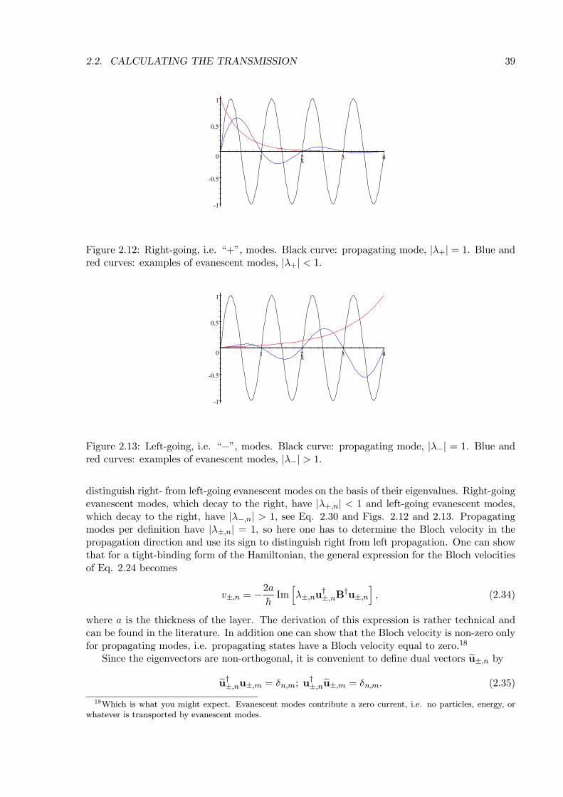
2.2. CALCULATING THE TRANSMISSION 39
-1
-0.5
0
0.5
1
1 2 3 4x
Figure 2.12: Right-going, i.e. “+”, modes. Black curve: propagating mode, |λ+| = 1. Blue andred curves: examples of evanescent modes, |λ+| < 1.
-1
-0.5
0
0.5
1
1 2 3 4x
Figure 2.13: Left-going, i.e. “−”, modes. Black curve: propagating mode, |λ−| = 1. Blue andred curves: examples of evanescent modes, |λ−| > 1.
distinguish right- from left-going evanescent modes on the basis of their eigenvalues. Right-goingevanescent modes, which decay to the right, have |λ+,n| < 1 and left-going evanescent modes,which decay to the right, have |λ−,n| > 1, see Eq. 2.30 and Figs. 2.12 and 2.13. Propagatingmodes per definition have |λ±,n| = 1, so here one has to determine the Bloch velocity in thepropagation direction and use its sign to distinguish right from left propagation. One can showthat for a tight-binding form of the Hamiltonian, the general expression for the Bloch velocitiesof Eq. 2.24 becomes
v±,n = −2ahImhλ±,nu†±,nB
†u±,ni, (2.34)
where a is the thickness of the layer. The derivation of this expression is rather technical andcan be found in the literature. In addition one can show that the Bloch velocity is non-zero onlyfor propagating modes, i.e. propagating states have a Bloch velocity equal to zero.18
Since the eigenvectors are non-orthogonal, it is convenient to define dual vectors eu±,n byeu†±,nu±,m = δn,m; u
†±,neu±,m = δn,m. (2.35)
18Which is what you might expect. Evanescent modes contribute a zero current, i.e. no particles, energy, orwhatever is transported by evanescent modes.
40 CHAPTER 2. ELECTRON TRANSPORT IN THREE DIMENSIONS
Any wave function in the leads can be expressed as a linear combination of the lead modes. Thiscan be done in a very compact way by defining the two N ×N Bloch matrices for right- andleft-going modes
F± =NXn=1
λ±,nu±,neu†±,n. (2.36)
These are the generalizations of the Bloch factors of the one-dimensional case, see Eqs. 1.100and 1.102. Note that one can easily construct powers of Bloch matrices
Fi± =NXn=1
λi±,nu±,neu†±,n. (2.37)
This is valid for any integer i, due to Eq. 2.35. A general solution in the leads can now beexpressed as a recursion relation
ci = c+,i + c−,i = Fi−j+ c+,j +Fi−j− c−,j . (2.38)
In a scattering problem one usually fixes the coefficients in one layer using boundary conditions.By using Eq. 2.38 one can then determine the solution in all the layers of the leads.
2.2.2 Mode matching
One can use these recursion relations to set up a set of equations that properly match the leadsto the scattering region. The scattering region is defined by the layers i = 1, . . . , S, see Fig.2.11. Immediately left of the scattering regions one has the recursion relation
c−1 = F−1L,+c+,0 +F−1L,−c−,0.
Writing c−,0 = c0 − c+,0 one gets
c−1 =hF−1L,+ −F−1L,−
ic+,0 +F
−1L,−c0. (2.39)
The scattering boundary condition is introduced in the following way. The vector c+,0 is treatedas the source, i.e. as the incoming wave from the left lead, e.g. a specific (propagating) modeof the left lead.
c+,0 = uL,+,m. (2.40)
Immediately right of the scattering region one has
cS+2 = FR,+c+,S+1 +FR,−c−,S+1.
Here the scattering boundary condition states that we have no incoming wave from the rightlead, i.e. c−,S+1 = 0, so
cS+2 = FR,+cS+1. (2.41)
The relations Eqs. 2.39 and 2.41 can now be used to “simplify” the tight-binding equations
−Bici−1 + (E1−Hi)ci −B†ici+1 = 0. (2.42)
2.2. CALCULATING THE TRANSMISSION 41
Ordinarily i runs from −∞ to ∞, but for i = 0 we can write
−BLc−1 + (E1−HL)c0 −B†1c1 = 0⇔(E1−HL −BLF−1L,−)c0 −B†1c1 = BL
hF−1L,+ −F−1L,−
iuL,+,m. (2.43)
Likewise one can write for i = S + 1
−BScS + (E1−HR)cS+1 −B†RcS+2 = 0⇔−BScS + (E1−HR −B†RFR,+)cS+1 = 0. (2.44)
Eq. 2.42, for i = 1, . . . , S, and Eqs. 2.43 and 2.44 can be collected into
(E1−H0)ψ = QL,+,m, (2.45)
with
H0 =
HL +ΣL(E) B†1 0 0 0
B1. . . B†i−1 0 0
0 Bi−1 Hi B†i 0
0 0 Bi. . . B†S
0 0 0 BS HR +ΣR(E)
, (2.46)
and
ψ =
c0...ci...
cS+1
; QL,+,m =
BL
hF−1L,+ −F−1L,−
iuL,+,m
...0...0
. (2.47)
The quantities
ΣL(E) = BLF−1L,−;
ΣR(E) = B†RFR,+, (2.48)
are called the self-energies of the left and right leads, respectively, just as in Eq. 1.107. Theycontain all the information about the coupling of the scattering region to the leads, as well as theinformation about the scattering boundary conditions. Note that the self-energies depend uponthe energy E, since are expressed in the Bloch matrices and thus in the lead modes and thelatter have been determined at a fixed energy E. Moreover, the self-energies are non-Hermitian,which makes the HamiltonianH0 non-Hermitian.19 An important observation is that Eq. 2.45has a finite dimension!20
Eq. 2.45 represents a set of linear equations of dimension (S + 2)×N . These can be solvedusing the common techniques, e.g. Gaussian elimination (or LU decomposition, as it is also
19This is logical if you know your quantum mechanics. A particle in the scattering region has a finite probabilityto leak into the leads, i.e. to disappear from the scattering region. In other words, the particle has a finite lifetime.This can only be expressed by non-Hermitian “Hamiltonians”, as Hermitian ones would only give real energies
and time factors e−ihEt yielding constant probabilities, i.e. infinite lifetimes.
20If you suspect that the “partitioning technique” is behind this, you are right.
42 CHAPTER 2. ELECTRON TRANSPORT IN THREE DIMENSIONS
known), followed by back substitution. Since the matrix H0 has a block tridiagonal form (theblocks being of dimension N), one can make use of this special form to make the Gaussianelimination algorithm efficient. The details can be found in the literature. Transmissionmatrix elements are obtained by expanding the wave function in the right lead into modes21
cS+1 =NXn−1
uR,+,nt0n,m ⇒ t0n,m = eu†R,+,ncS+1 (2.49)
and normalize them with the velocities to ensure a unitary scattering matrix, see Eqs. 1.53 and1.72.
tn,m =
rvL,+,mvR,+,n
eu†R,+,ncS+1 (2.50)
The velocities are calculated from Eq. 2.34.By letting m in Eqs. 2.40 and 2.47 run over all (propagating) modes uL,+,m of the left lead,
all transmission matrix elements can be obtained. This sounds actually more complicated thanit is. Gaussian elimination (LU decomposition) is the most time consuming algorithmic stepin solving the linear equations of Eq. 2.45. This step however is independent of QL,+,m. Thelatter only enters in the second algorithmic step, i.e. back substitution, which is much cheaperand is performed for each QL,+,m. Moreover, the back substitution step does not have to becomplete, since only the coefficients cS+1 are needed to calculate the transmission.
22
Although the mode matching formalism allows for calculating t0n,m matrix elements accordingto Eq. 2.49 between all states n and m, i.e. propagating states and evanescent states, onlypropagating states contribute to the transmission. In this sense it is allowed to restrict n andm to the propagating states only. This does not mean that one can throw out the evanescentstates altogether, though. One needs to include them in properly matching the scattering regionto the leads, cf. Eq. 2.48. In other words, the Bloch matrices, Eq. 2.37, need to be constructedfrom all N modes, propagating and evanescent.23 Both of them are needed for a complete basis.
2.2.3 Green function expressions
For those of you who cannot live without Green functions, I can give you the Landauer formalismexpressed in Green functions. The derivations are rather technical, so I will skip most of them.You can find them in the literature. With respect to the Hamiltonian matrix of Eq. 2.46 a finiteGreen function matrix can be defined as
G(E) = (E1−H0)−1. (2.51)
It can be calculated by matrix inversion using essentially the same block Gaussian eliminationscheme as in solving the set of linear equations, Eq. 2.45. The matrix H0 is non-Hermitian; itseigenvalues are not real, so the Green function matrix can be evaluated for real energies.24
With respect to the original infinite Hamiltonian H of Eq. 2.27 one can define the usualretarded (infinite) Green function matrix
Gr(E) = [(E + iη)1−H]−1 , (2.52)
21Again, replace n by kkn or kknσ, when appropriate.22However, if one wants to have the full wave function ψ or calculate the reflection coefficients, the back
transformation has to be complete. It is not expensive, though (compared to the Gaussian elimination step).23Only the full set forms a complete basis.24The exceptions are truly bound states ofH0. These occur at real energies, at which the Green function matrix
thus has poles. However, these occur outside the energy range that is of interest for scattering. At bound stateenergies only evanescent modes exist in the leads, so this situation is easily identified in practice.
2.2. CALCULATING THE TRANSMISSION 43
where one needs the infinitesimal η to avoid the poles on the real axis. The advanced Greenfunction Ga(E) can be obtained from Eq. 1.80. One can show that for layers in the scatteringregion one has
Gi,j(E) = Gri,j(E); i, j = 0, . . . , S + 1. (2.53)
if one properly takes the limη→0. In terms of the Green function, the wave function in thescattering region can be written as
ψ =G(E) QL,+,m, (2.54)
and from Eq. 2.49 one obtains
tn,m =
rvL,+,mvR,+,n
eu†R,+,n GS+1,0(E) QL,+,m. (2.55)
After some manipulation one can obtain a Fisher-Lee expression that generalizes the 1Dexpression of Eq. 1.83
tn,m = ih
rvR,+,nvL,+,m
aLaReu†R,+,n GS+1,0(E) eu0L,+,m. (2.56)
The notation is a bit messy due to the fact the modes uL/R,+,m/n are not orthogonal; see Sec.
2.2.1. If they were orthogonal, then the expression would simply contain u†R,+,nGS+1,0(E)uL,+,m.This indicates that the transmission amplitude from mode uL,+,m in the left lead to mode uR,+,nin the right lead is determined by the Green function matrix that brings you from layer i = 0to layer i = S + 1, i.e. across the scattering region. Proper orthogonalization of the modesleads to expressions for eu†R,+,n and eu0L,+,m. The details are a bit messy and can be found in theliterature. The Bloch velocities vL/R,+,m/n serve to make scattering matrix unitary, as before.Since vL/R,+,m/n 6= 0 only for propagating states, Eq. 2.56 expresses explicitly that the trans-mission is zero whenever n or m describes an evanescent mode. The layer thicknesses aL/R arejust normalization factors, since our modes are normalized within a layer.
After some algebra the Green function expressions we obtained in the one-dimensional casecan be generalized to three dimensions. The velocity of Eq. 1.77 becomes a velocity matrix
VL/R = −2aL/R
hImΣL/R. (2.57)
It is a diagonal matrix of dimension N (the total number of modes). The diagonal matrixelements are the mode velocities vL/R,±,n of Eq. 2.34. Since vL/R,±,n = 0 for evanescent states,this means that in general the velocity matrices are singular. The transmission amplitudes ofEq. 2.56 can be assembled in a transmission matrix t, which using the velocity matrices can beexpressed as
t = 2ip− ImΣR GS+1,0(E)
p− ImΣL. (2.58)
Note that this generalizes Eq. 1.84. Finally, the total transmission can be expressed as
T = Trht†ti= 4Tr
£ImΣR G
rS+1,0(E) ImΣL G
a0,S+1(E)
¤(2.59)
which generalizes Eq. 1.85. This is known as the Caroli expression or the NEGF expres-sion.25
25NEGF = non-equilibrium Green function. In the linear response regime one can use equilirium Green func-tions, however, which is what we are doing here.


![Theory of Electron, Phonon and Spin Transport in Nanoscale ... · kinetic theory of quantum transport [15], scattering theory [16] and master equation approach [17]. In this paper,](https://img.pdfslide.us/doc/110x75/5fc76cdd99a943642b6a3adb/theory-of-electron-phonon-and-spin-transport-in-nanoscale-kinetic-theory-of.jpg)