Embed Size (px)
Citation preview
DePaul University DePaul University
Via Sapientiae Via Sapientiae
College of Science and Health Theses and Dissertations College of Science and Health
Summer 8-22-2021
ANALYZING NANOSCALE THERMAL TRANSPORT USING TIME-ANALYZING NANOSCALE THERMAL TRANSPORT USING TIME-
RESOLVED X-RAY DIFFRACTION RESOLVED X-RAY DIFFRACTION
James Grammich DePaul University, [email protected]
Follow this and additional works at: https://via.library.depaul.edu/csh_etd
Part of the Physics Commons
Recommended Citation Recommended Citation Grammich, James, "ANALYZING NANOSCALE THERMAL TRANSPORT USING TIME-RESOLVED X-RAY DIFFRACTION" (2021). College of Science and Health Theses and Dissertations. 387. https://via.library.depaul.edu/csh_etd/387
This Thesis is brought to you for free and open access by the College of Science and Health at Via Sapientiae. It has been accepted for inclusion in College of Science and Health Theses and Dissertations by an authorized administrator of Via Sapientiae. For more information, please contact [email protected].
ANALYZING NANOSCALE THERMAL TRANSPORT USINGTIME-RESOLVED X-RAY DIFFRACTION
A Thesis
Presented in
Partial Fulfillment of the
Requirements for the Degree of
MASTER OF SCIENCE
2 0 2 1
BY
James Grammich
PHYSICS DEPARTMENT
College of Science and Health
DePaul University
Chicago, Illinois
2
ACKNOWLEDGEMENTS
I would like to thank Dr. Eric Landahl for being my advisor during my timehere at DePaul. In addition to helping me with this project, Dr. Landahl hashelped me to become a better scientist. Additionally, I would also like to thankDr. Bernhard Beck-Winchatz and Dr. Gabriela Gonzalez Aviles for serving on mythesis committee.
The initial version of the TRXD code was written by former DePaul Physicsgraduate student Dr. G. Jackson Williams (now at Lawrence Livermore NationalLaboratory), and further developed by Dr. Landahl. Initial tests of the code wereconducted by DePaul Physics undergraduate students Danielle Leppert-Simenauerand Sinead Humphrey. Data analyzed in this experiment was taken by DePaulPhysics undergraduate students Grace Longbons and Timothy Holmes, along withDr. Landahl, Dr. Don Walko (Argonne National Laboratory), Dr. WonHyuk Jo(now at DESY), and Dr. Sooheyong Lee (KRISS). Samples were provided by KRISS.
Benchmarking of TRXD in this study was performed using program GID SL atSergey Stepanov’s X-Ray Server, https://x-server.gmca.aps.anl.gov .
Use of the Advanced Photon Source was supported by the U.S. Department ofEnergy, Basic Energy Sciences, Office of Science, under Contract No. DE-AC02-06CH11357.
I would like to thank everyone at the DePaul Physics department. You have allhelped me grow tremendously, and made my time here immensely enjoyable.
Lastly, I want to thank all of my family and friends outside of DePaul who haveprovided me with support and encouragement these past few years.
3
TABLE OF CONTENTS
LIST OF FIGURES . . . . . . . . . . . . . . . . . . . . . . . . . . . . 4
LIST OF TABLES . . . . . . . . . . . . . . . . . . . . . . . . . . . . . 9
ABSTRACT . . . . . . . . . . . . . . . . . . . . . . . . . . . . . . . . . 10
CHAPTER 1 Introduction . . . . . . . . . . . . . . . . . . . . . . . . 111.1 Thesis motivation . . . . . . . . . . . . . . . . . . . . . . . . . . . . . 111.2 Classical theory of heat transport . . . . . . . . . . . . . . . . . . . . 13
1.2.1 Overview . . . . . . . . . . . . . . . . . . . . . . . . . . . . . 131.2.2 Solving the diffusion equation . . . . . . . . . . . . . . . . . . 151.2.3 Example of the classical heat conduction result . . . . . . . . 17
1.3 Nanoscale thermal transport and the phonon mean free path . . . . . 18
CHAPTER 2 Benchmarking diffraction calculations . . . . . . . . 222.1 Chapter introduction . . . . . . . . . . . . . . . . . . . . . . . . . . . 222.2 X-ray diffraction as a temperature probe . . . . . . . . . . . . . . . . 222.3 Dynamical diffraction . . . . . . . . . . . . . . . . . . . . . . . . . . . 232.4 Dynamical diffraction calculations . . . . . . . . . . . . . . . . . . . . 242.5 Code benchmarking . . . . . . . . . . . . . . . . . . . . . . . . . . . . 25
CHAPTER 3 Comparison to experiment . . . . . . . . . . . . . . . 303.1 Chapter introduction . . . . . . . . . . . . . . . . . . . . . . . . . . . 303.2 Time-resolved x-ray diffraction experiment . . . . . . . . . . . . . . . 303.3 Data reduction . . . . . . . . . . . . . . . . . . . . . . . . . . . . . . 333.4 Convolution with instrument resolution . . . . . . . . . . . . . . . . . 43
CHAPTER 4 Agreement and discrepancy with classical theory . . 464.1 Observed behavior . . . . . . . . . . . . . . . . . . . . . . . . . . . . 50
CHAPTER 5 Discussion, summary, and outlook . . . . . . . . . . . 645.1 New information on nanoscale thermal transport . . . . . . . . . . . . 645.2 Thesis summary . . . . . . . . . . . . . . . . . . . . . . . . . . . . . . 645.3 Outlook . . . . . . . . . . . . . . . . . . . . . . . . . . . . . . . . . . 66
APPENDIX A MATLAB codes . . . . . . . . . . . . . . . . . . . . . 67
4
LIST OF FIGURES
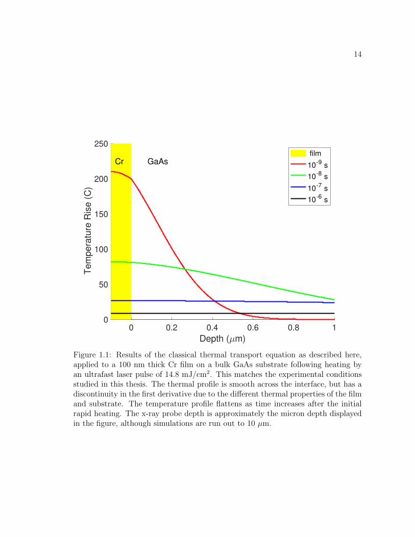
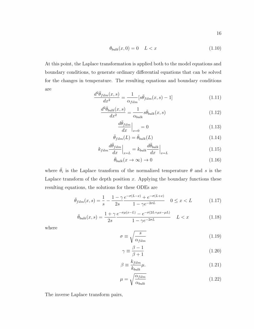
1.1 Results of the classical thermal transport equation as described here,applied to a 100 nm thick Cr film on a bulk GaAs substrate followingheating by an ultrafast laser pulse of 14.8 mJ/cm2. This matches theexperimental conditions studied in this thesis. The thermal profileis smooth across the interface, but has a discontinuity in the firstderivative due to the different thermal properties of the film and sub-strate. The temperature profile flattens as time increases after theinitial rapid heating. The x-ray probe depth is approximately themicron depth displayed in the figure, although simulations are runout to 10 µm. . . . . . . . . . . . . . . . . . . . . . . . . . . . . . . 14
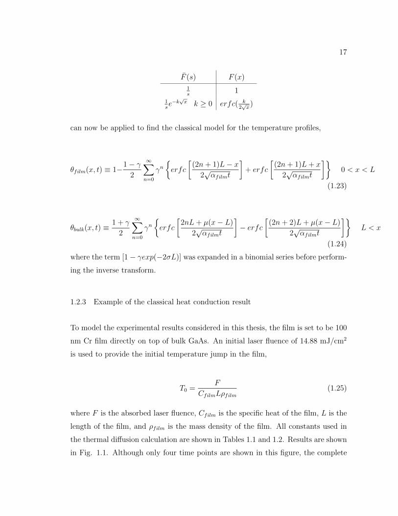
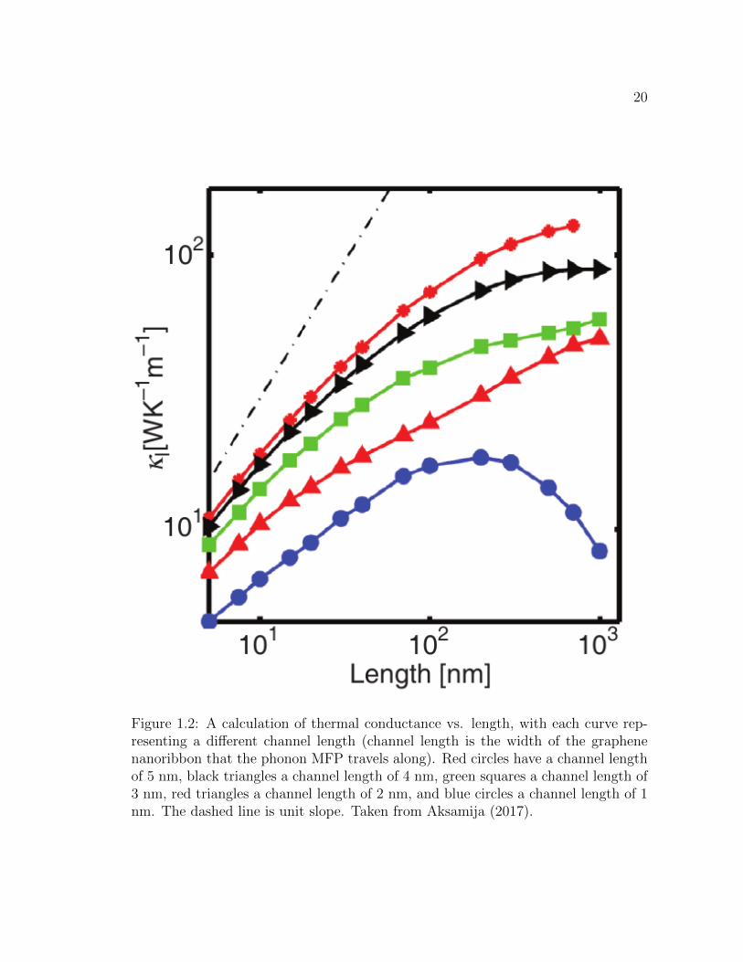
1.2 A calculation of thermal conductance vs. length, with each curverepresenting a different channel length (channel length is the widthof the graphene nanoribbon that the phonon MFP travels along).Red circles have a channel length of 5 nm, black triangles a channellength of 4 nm, green squares a channel length of 3 nm, red trianglesa channel length of 2 nm, and blue circles a channel length of 1 nm.The dashed line is unit slope. Taken from Aksamija (2017). . . . . . . 20
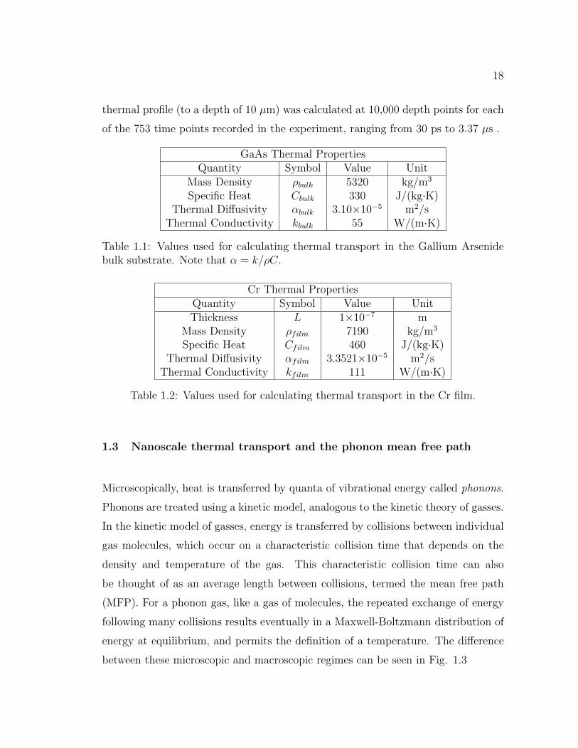
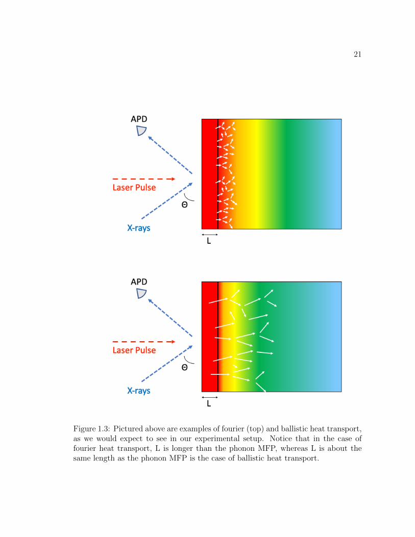
1.3 Pictured above are examples of fourier (top) and ballistic heat trans-port, as we would expect to see in our experimental setup. Noticethat in the case of fourier heat transport, L is longer than the phononMFP, whereas L is about the same length as the phonon MFP is thecase of ballistic heat transport. . . . . . . . . . . . . . . . . . . . . . 21
2.1 Data analysis and modelling procedure. We begin by putting our in-formation into TRXD (timepoints, angular ranges for rocking curvecalculations, material constants, and laser fluence), which producesstrain profiles that are used in turn to find the rocking curves ex-pected from the classical model. Next the centroids are compared tothe rocking curve data collected before time zero, which is used to de-termine the average temperature change using the thermal expansioncoefficient. . . . . . . . . . . . . . . . . . . . . . . . . . . . . . . . . . 25
2.2 Linear scale comparison ofTRXD and GID SL for a test case of 0.01%uniform strain over the first 2 µm of depth in GaAs [004] reflectionat 10 keV. The unstrained crystal result is shown for reference. . . . . 27
LIST OF FIGURES – Continued
5
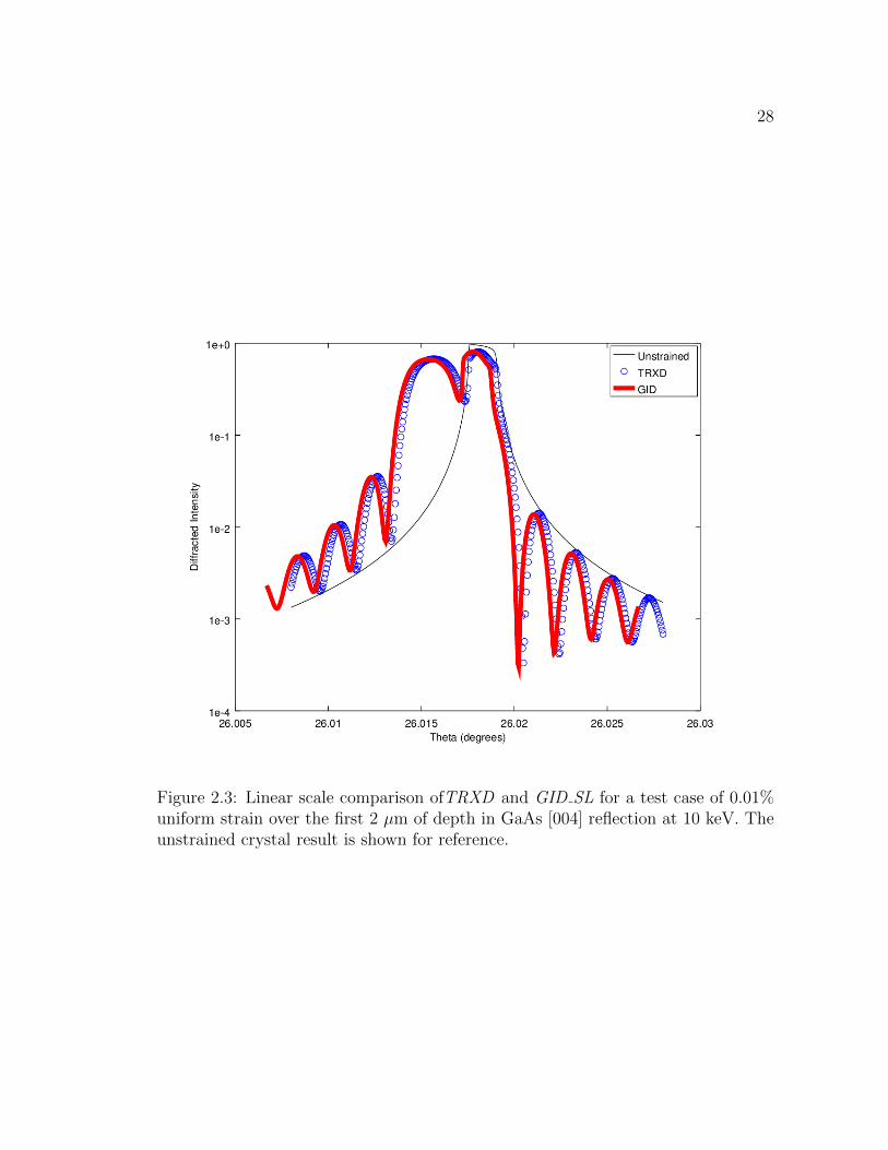
2.3 Linear scale comparison ofTRXD and GID SL for a test case of 0.01%uniform strain over the first 2 µm of depth in GaAs [004] reflectionat 10 keV. The unstrained crystal result is shown for reference. . . . . 28
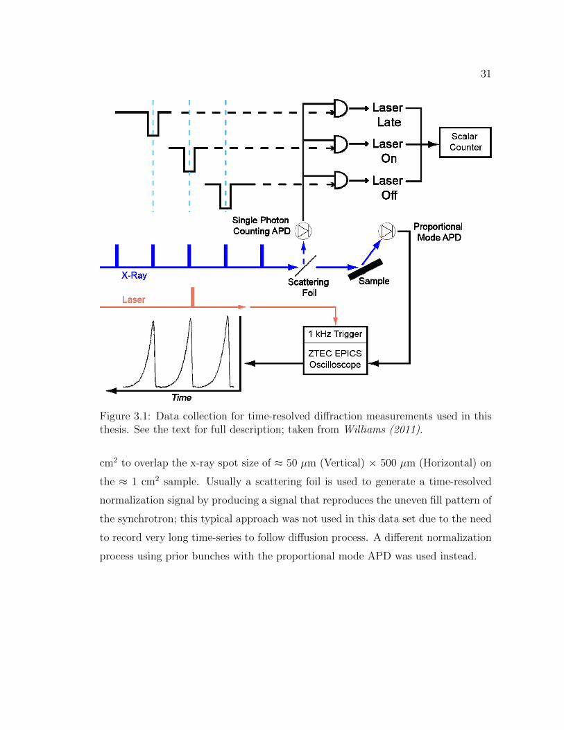
3.1 Data collection for time-resolved diffraction measurements used inthis thesis. See the text for full description; taken from Williams(2011). . . . . . . . . . . . . . . . . . . . . . . . . . . . . . . . . . . . 31
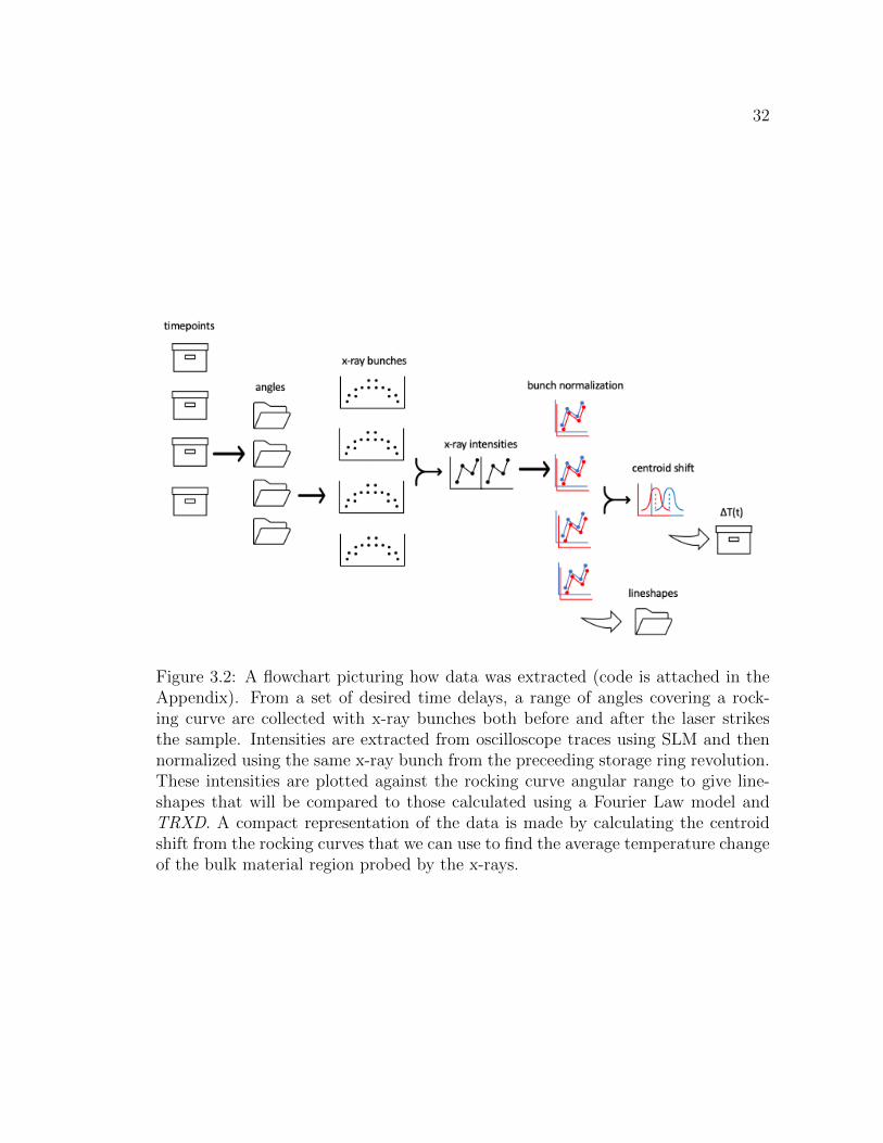
3.2 A flowchart picturing how data was extracted (code is attached inthe Appendix). From a set of desired time delays, a range of anglescovering a rocking curve are collected with x-ray bunches both beforeand after the laser strikes the sample. Intensities are extracted fromoscilloscope traces using SLM and then normalized using the samex-ray bunch from the preceeding storage ring revolution. These in-tensities are plotted against the rocking curve angular range to givelineshapes that will be compared to those calculated using a FourierLaw model and TRXD. A compact representation of the data is madeby calculating the centroid shift from the rocking curves that we canuse to find the average temperature change of the bulk material regionprobed by the x-rays. . . . . . . . . . . . . . . . . . . . . . . . . . . . 32
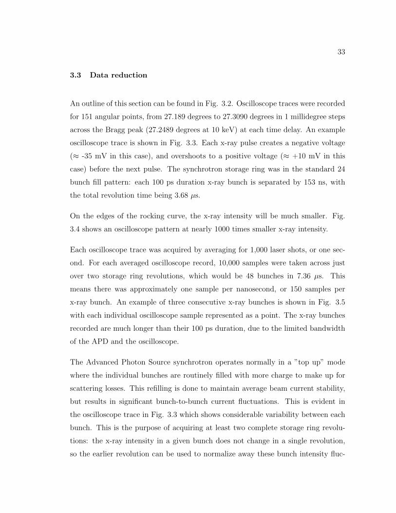
3.3 Avalanche Photodiode (APD) detector response to just over two stor-age ring rotations (the data was taken twice - once with and oncewithout the laser heating our sample) in the standard 24 bunch op-erating mode. This data was recorded following diffraction from alaser-excited sample, near the peak of the Bragg diffraction peak. . . 34
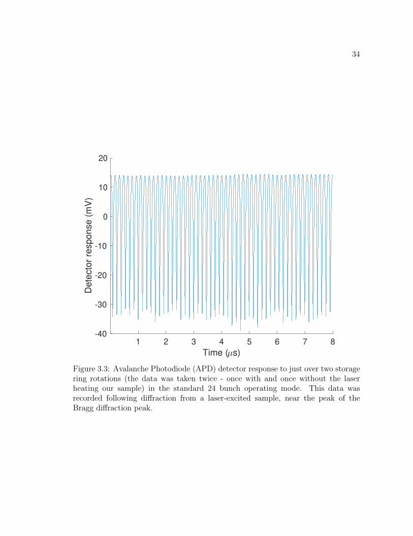
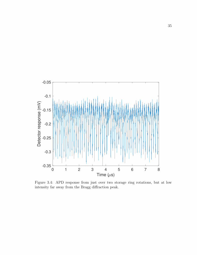
3.4 APD response from just over two storage ring rotations, but at lowintensity far away from the Bragg diffraction peak. . . . . . . . . . . 35
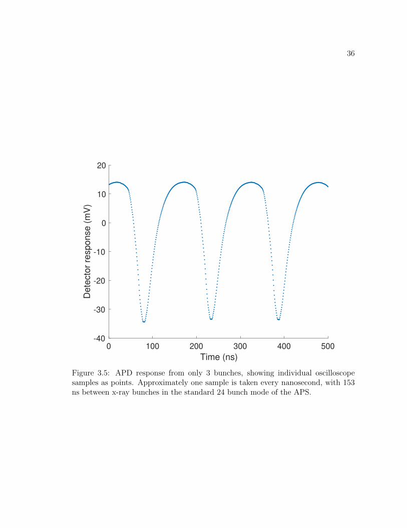
3.5 APD response from only 3 bunches, showing individual oscilloscopesamples as points. Approximately one sample is taken every nanosec-ond, with 153 ns between x-ray bunches in the standard 24 bunchmode of the APS. . . . . . . . . . . . . . . . . . . . . . . . . . . . . . 36
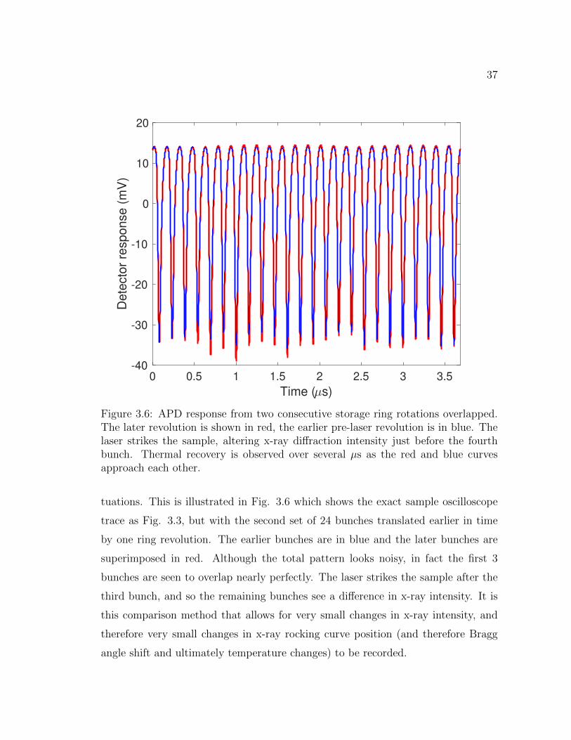
3.6 APD response from two consecutive storage ring rotations over-lapped. The later revolution is shown in red, the earlier pre-laserrevolution is in blue. The laser strikes the sample, altering x-raydiffraction intensity just before the fourth bunch. Thermal recoveryis observed over several µs as the red and blue curves approach eachother. . . . . . . . . . . . . . . . . . . . . . . . . . . . . . . . . . . . 37
LIST OF FIGURES – Continued
6
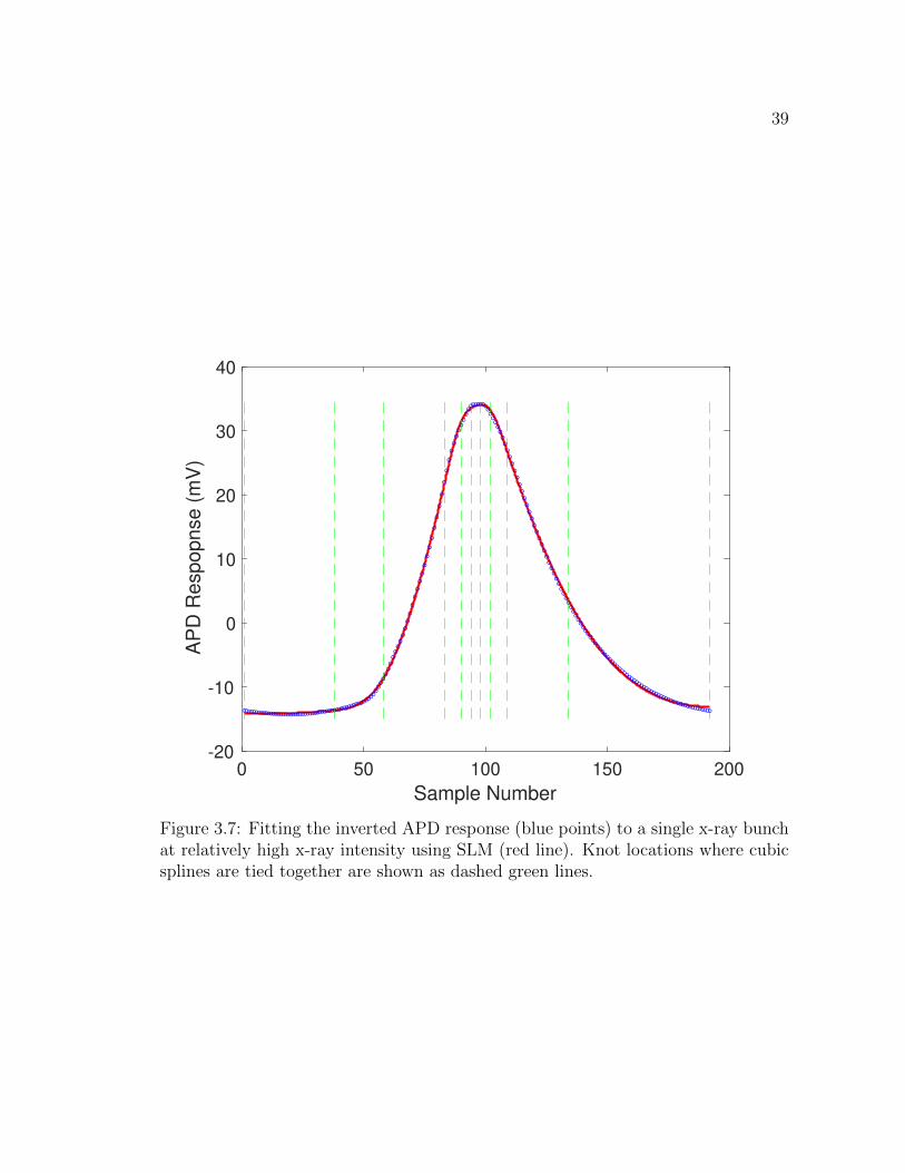
3.7 Fitting the inverted APD response (blue points) to a single x-raybunch at relatively high x-ray intensity using SLM (red line). Knotlocations where cubic splines are tied together are shown as dashedgreen lines. . . . . . . . . . . . . . . . . . . . . . . . . . . . . . . . . 39
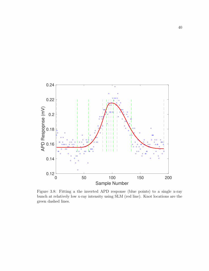
3.8 Fitting a the inverted APD response (blue points) to a single x-raybunch at relatively low x-ray intensity using SLM (red line). Knotlocations are the green dashed lines. . . . . . . . . . . . . . . . . . . 40
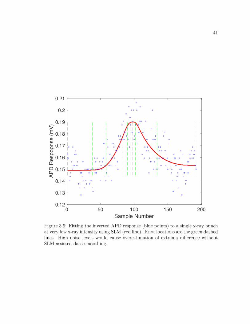
3.9 Fitting the inverted APD response (blue points) to a single x-raybunch at very low x-ray intensity using SLM (red line). Knot loca-tions are the green dashed lines. High noise levels would cause over-estimation of extrema difference without SLM-assisted data smoothing. 41
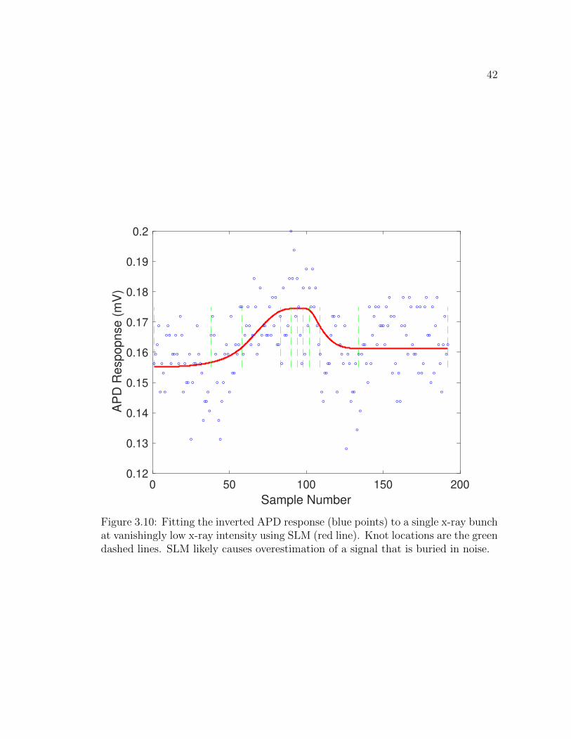
3.10 Fitting the inverted APD response (blue points) to a single x-raybunch at vanishingly low x-ray intensity using SLM (red line). Knotlocations are the green dashed lines. SLM likely causes overestimationof a signal that is buried in noise. . . . . . . . . . . . . . . . . . . . . 42
3.11 TRXD unstrained rocking curve theoretical calculation (dashed line),the Voigt profile instrument resolution function (dotted line), and thetheoretical calculation convolved with the instrument resolution (solidline) compared with unstrained [400] GaAs rocking curve measure-ment at 10 keV (circles). . . . . . . . . . . . . . . . . . . . . . . . . . 45
4.1 Classical thermal film model rocking curve centroids (calculated usingTRXD, black line) and data (red circles) for a 14.88 mJ/cm2 absorbedlaser fluence on 100 nm thick Cr deposited on bulk GaAs at 10 keV.The top figure is linear in time, the lower figure is on a logarithmictime scale. The inset in the top figure shows data and model neart = 0. Temperature shifts are calculated from centroid shifts usingEq. 2.3. . . . . . . . . . . . . . . . . . . . . . . . . . . . . . . . . . . 47
LIST OF FIGURES – Continued
7
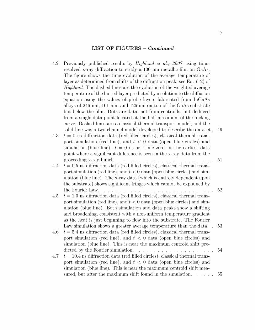
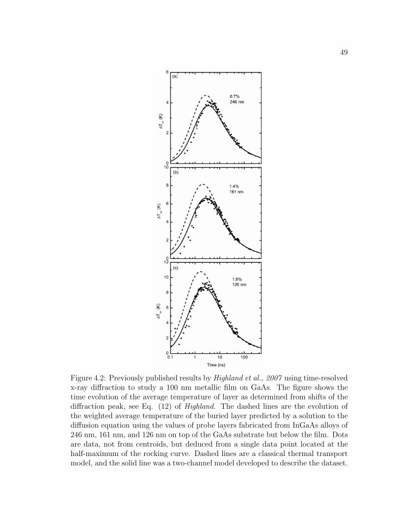
4.2 Previously published results by Highland et al., 2007 using time-resolved x-ray diffraction to study a 100 nm metallic film on GaAs.The figure shows the time evolution of the average temperature oflayer as determined from shifts of the diffraction peak, see Eq. (12) ofHighland. The dashed lines are the evolution of the weighted averagetemperature of the buried layer predicted by a solution to the diffusionequation using the values of probe layers fabricated from InGaAsalloys of 246 nm, 161 nm, and 126 nm on top of the GaAs substratebut below the film. Dots are data, not from centroids, but deducedfrom a single data point located at the half-maximum of the rockingcurve. Dashed lines are a classical thermal transport model, and thesolid line was a two-channel model developed to describe the dataset. 49
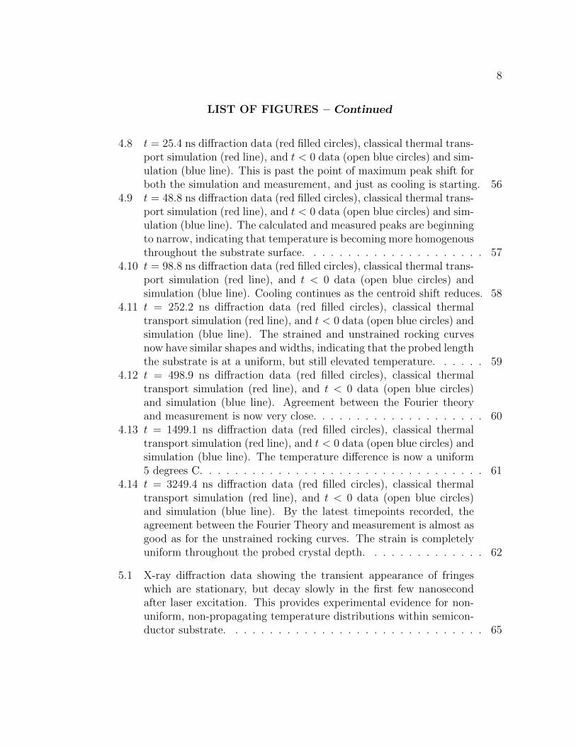
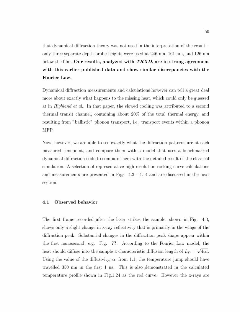
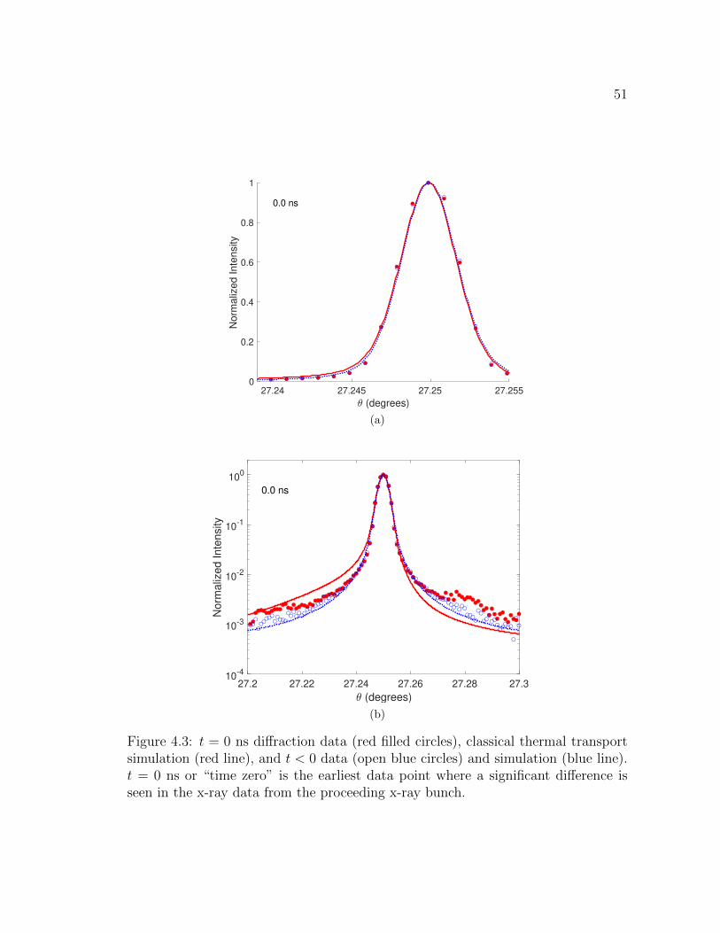
4.3 t = 0 ns diffraction data (red filled circles), classical thermal trans-port simulation (red line), and t < 0 data (open blue circles) andsimulation (blue line). t = 0 ns or “time zero” is the earliest datapoint where a significant difference is seen in the x-ray data from theproceeding x-ray bunch. . . . . . . . . . . . . . . . . . . . . . . . . . 51
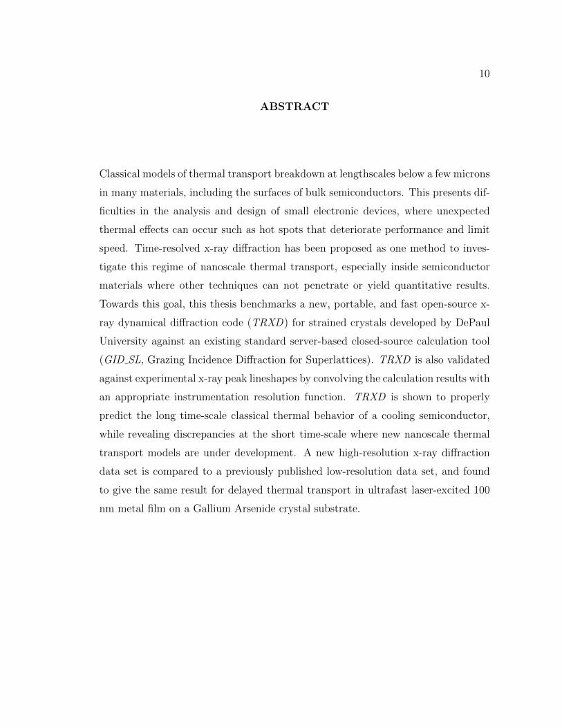
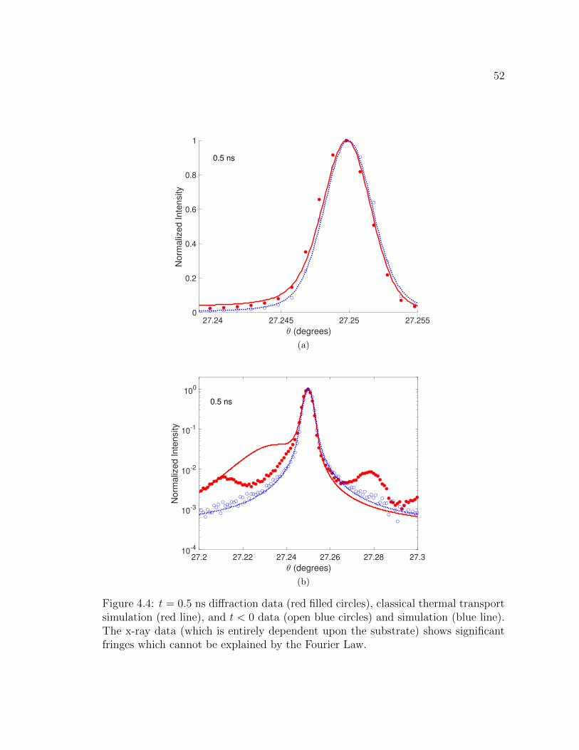
4.4 t = 0.5 ns diffraction data (red filled circles), classical thermal trans-port simulation (red line), and t < 0 data (open blue circles) and sim-ulation (blue line). The x-ray data (which is entirely dependent uponthe substrate) shows significant fringes which cannot be explained bythe Fourier Law. . . . . . . . . . . . . . . . . . . . . . . . . . . . . . 52
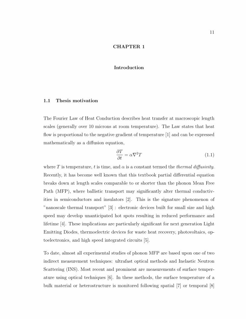
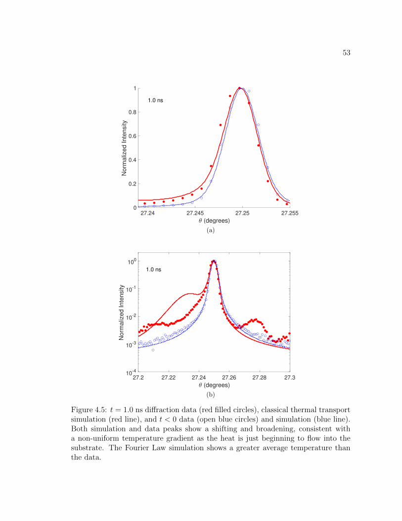
4.5 t = 1.0 ns diffraction data (red filled circles), classical thermal trans-port simulation (red line), and t < 0 data (open blue circles) and sim-ulation (blue line). Both simulation and data peaks show a shiftingand broadening, consistent with a non-uniform temperature gradientas the heat is just beginning to flow into the substrate. The FourierLaw simulation shows a greater average temperature than the data. . 53
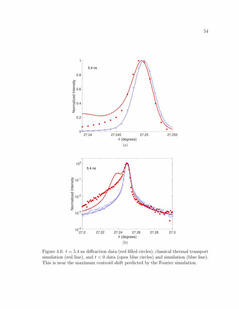
4.6 t = 5.4 ns diffraction data (red filled circles), classical thermal trans-port simulation (red line), and t < 0 data (open blue circles) andsimulation (blue line). This is near the maximum centroid shift pre-dicted by the Fourier simulation. . . . . . . . . . . . . . . . . . . . . 54
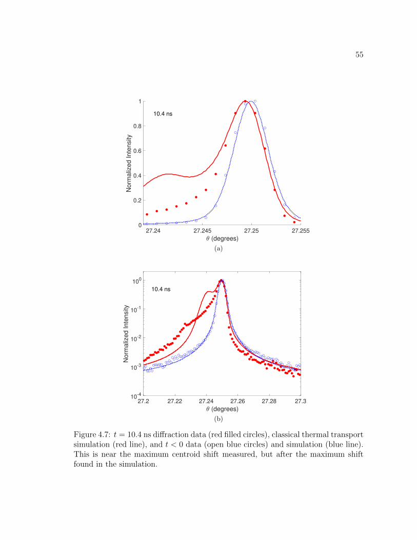
4.7 t = 10.4 ns diffraction data (red filled circles), classical thermal trans-port simulation (red line), and t < 0 data (open blue circles) andsimulation (blue line). This is near the maximum centroid shift mea-sured, but after the maximum shift found in the simulation. . . . . . 55
LIST OF FIGURES – Continued
8
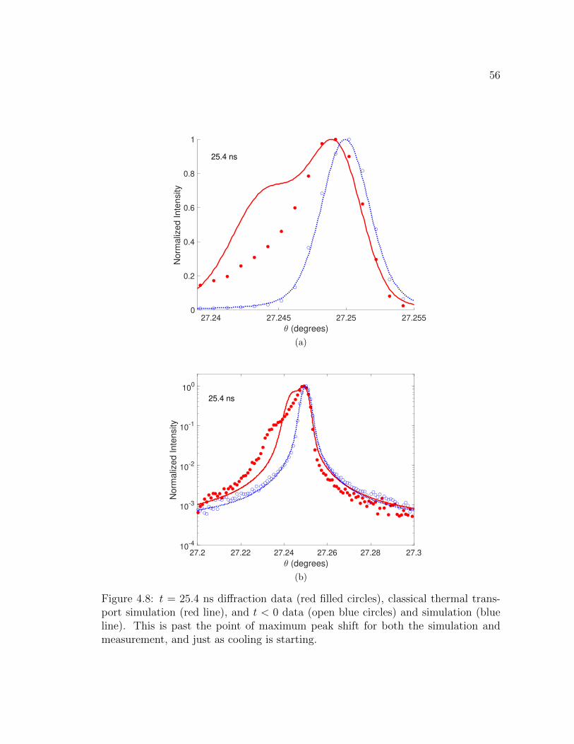
4.8 t = 25.4 ns diffraction data (red filled circles), classical thermal trans-port simulation (red line), and t < 0 data (open blue circles) and sim-ulation (blue line). This is past the point of maximum peak shift forboth the simulation and measurement, and just as cooling is starting. 56
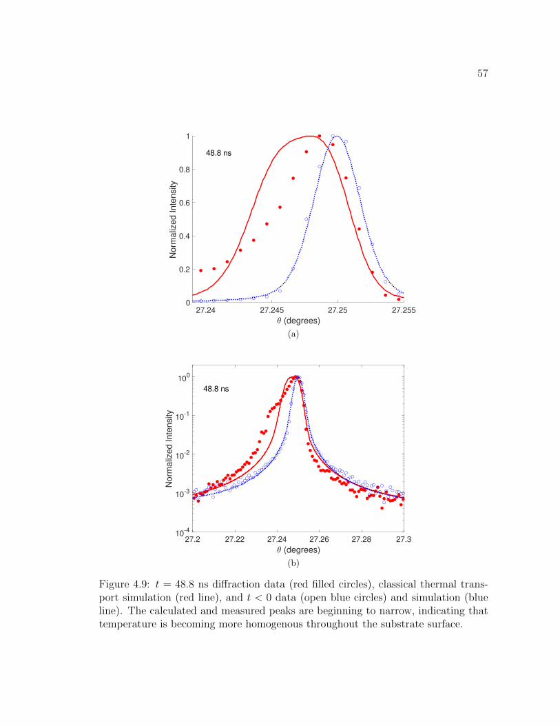
4.9 t = 48.8 ns diffraction data (red filled circles), classical thermal trans-port simulation (red line), and t < 0 data (open blue circles) and sim-ulation (blue line). The calculated and measured peaks are beginningto narrow, indicating that temperature is becoming more homogenousthroughout the substrate surface. . . . . . . . . . . . . . . . . . . . . 57
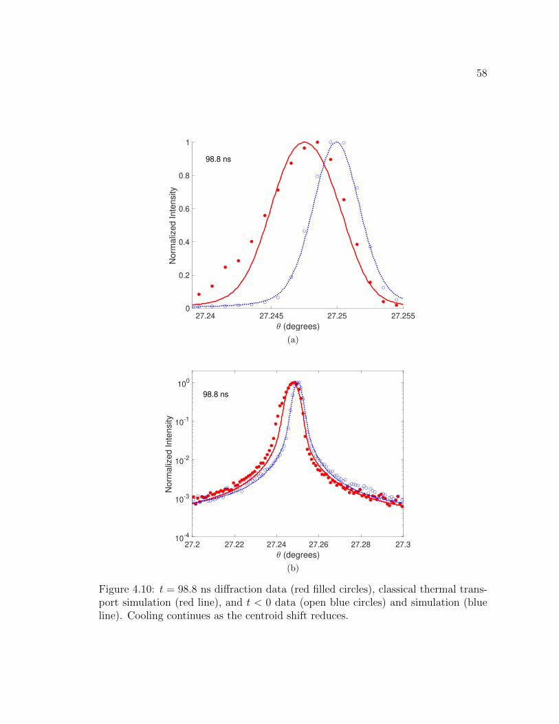
4.10 t = 98.8 ns diffraction data (red filled circles), classical thermal trans-port simulation (red line), and t < 0 data (open blue circles) andsimulation (blue line). Cooling continues as the centroid shift reduces. 58
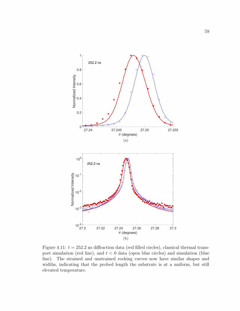
4.11 t = 252.2 ns diffraction data (red filled circles), classical thermaltransport simulation (red line), and t < 0 data (open blue circles) andsimulation (blue line). The strained and unstrained rocking curvesnow have similar shapes and widths, indicating that the probed lengththe substrate is at a uniform, but still elevated temperature. . . . . . 59
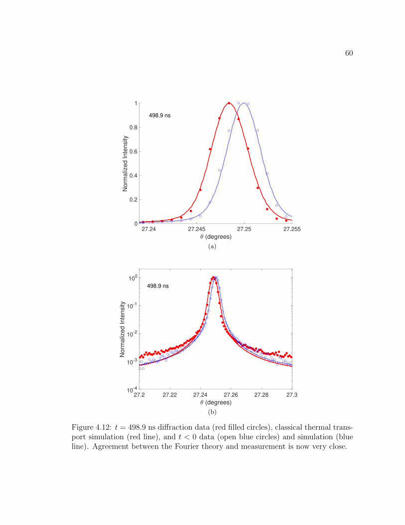
4.12 t = 498.9 ns diffraction data (red filled circles), classical thermaltransport simulation (red line), and t < 0 data (open blue circles)and simulation (blue line). Agreement between the Fourier theoryand measurement is now very close. . . . . . . . . . . . . . . . . . . . 60
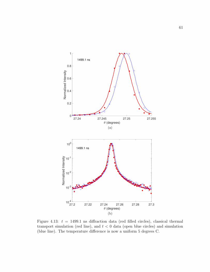
4.13 t = 1499.1 ns diffraction data (red filled circles), classical thermaltransport simulation (red line), and t < 0 data (open blue circles) andsimulation (blue line). The temperature difference is now a uniform5 degrees C. . . . . . . . . . . . . . . . . . . . . . . . . . . . . . . . . 61
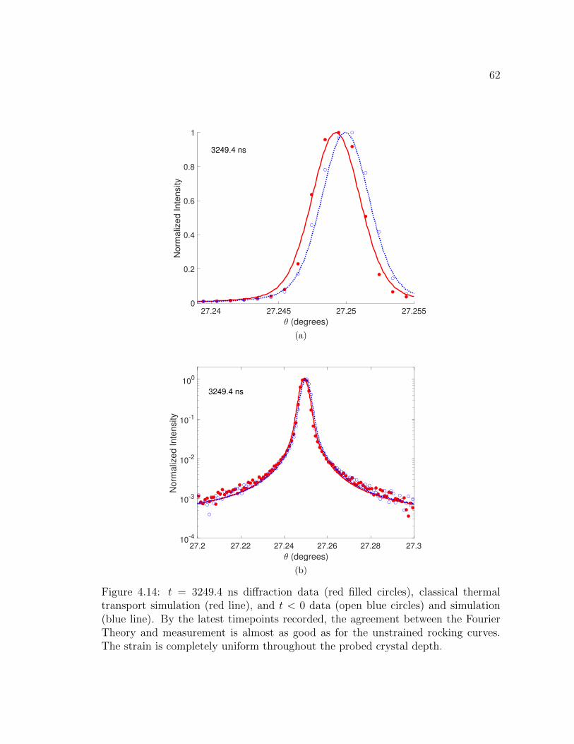
4.14 t = 3249.4 ns diffraction data (red filled circles), classical thermaltransport simulation (red line), and t < 0 data (open blue circles)and simulation (blue line). By the latest timepoints recorded, theagreement between the Fourier Theory and measurement is almost asgood as for the unstrained rocking curves. The strain is completelyuniform throughout the probed crystal depth. . . . . . . . . . . . . . 62
5.1 X-ray diffraction data showing the transient appearance of fringeswhich are stationary, but decay slowly in the first few nanosecondafter laser excitation. This provides experimental evidence for non-uniform, non-propagating temperature distributions within semicon-ductor substrate. . . . . . . . . . . . . . . . . . . . . . . . . . . . . . 65

9
LIST OF TABLES
1.1 Values used for calculating thermal transport in the Gallium Arsenidebulk substrate. Note that α = k/ρC. . . . . . . . . . . . . . . . . . . 18
1.2 Values used for calculating thermal transport in the Cr film. . . . . . 18
10
ABSTRACT
Classical models of thermal transport breakdown at lengthscales below a few microns
in many materials, including the surfaces of bulk semiconductors. This presents dif-
ficulties in the analysis and design of small electronic devices, where unexpected
thermal effects can occur such as hot spots that deteriorate performance and limit
speed. Time-resolved x-ray diffraction has been proposed as one method to inves-
tigate this regime of nanoscale thermal transport, especially inside semiconductor
materials where other techniques can not penetrate or yield quantitative results.
Towards this goal, this thesis benchmarks a new, portable, and fast open-source x-
ray dynamical diffraction code (TRXD) for strained crystals developed by DePaul
University against an existing standard server-based closed-source calculation tool
(GID SL, Grazing Incidence Diffraction for Superlattices). TRXD is also validated
against experimental x-ray peak lineshapes by convolving the calculation results with
an appropriate instrumentation resolution function. TRXD is shown to properly
predict the long time-scale classical thermal behavior of a cooling semiconductor,
while revealing discrepancies at the short time-scale where new nanoscale thermal
transport models are under development. A new high-resolution x-ray diffraction
data set is compared to a previously published low-resolution data set, and found
to give the same result for delayed thermal transport in ultrafast laser-excited 100
nm metal film on a Gallium Arsenide crystal substrate.
11
CHAPTER 1
Introduction
1.1 Thesis motivation
The Fourier Law of Heat Conduction describes heat transfer at macroscopic length
scales (generally over 10 microns at room temperature). The Law states that heat
flow is proportional to the negative gradient of temperature [1] and can be expressed
mathematically as a diffusion equation,
∂T
∂t= α∇2T (1.1)
where T is temperature, t is time, and α is a constant termed the thermal diffusivity.
Recently, it has become well known that this textbook partial differential equation
breaks down at length scales comparable to or shorter than the phonon Mean Free
Path (MFP), where ballistic transport may significantly alter thermal conductiv-
ities in semiconductors and insulators [2]. This is the signature phenomenon of
”nanoscale thermal transport” [3] : electronic devices built for small size and high
speed may develop unanticipated hot spots resulting in reduced performance and
lifetime [4]. These implications are particularly significant for next generation Light
Emitting Diodes, thermoelectric devices for waste heat recovery, photovoltaics, op-
toelectronics, and high speed integrated circuits [5].
To date, almost all experimental studies of phonon MFP are based upon one of two
indirect measurement techniques: ultrafast optical methods and Inelastic Neutron
Scattering (INS). Most recent and prominent are measurements of surface temper-
ature using optical techniques [6]. In these methods, the surface temperature of a
bulk material or heterostructure is monitored following spatial [7] or temporal [8]
12
modulation of surface heating (usually with a short-pulse later). The bulk behavior
is then inferred from the surface temperature evolution. The time-dependent sur-
face temperature has been found to change depending upon modulation frequency;
the thermal conductivity value is seen to increase monotonically as the modula-
tion wavelength increases past the phonon mean free path. This ”accumulation”
method of phonon MFP spectroscopy has yielded several insights. For instance,
low-frequency phonons carry thermal energy very long distances, but rely on scat-
tering with high-frequency phonons to locally equilibrate [9]. Thus, details of the
phonon density of states (DOS) may have significant impact on the phonon lifetime,
and thereby the MFP and conductivity. This has brought about a renewed interest
in INS for phonon dispersion and lifetime measurements [10].
There are several limitations implicit in these methods. First, the optical tech-
niques only allow surface temperature to be measured. Deviations from the depth-
dependent temperature profile are presumed, but have not been verified. Second,
the exploration of transport across defects has been extremely limited, since the
accumulation techniques are not very sensitive to sub-surface modifications which
affect mostly high-frequency phonons which cannot be clearly isolated from the “ac-
cumulated” spectra. Third, the major technological issue associated with nanoscale
thermal transport are buried interfaces, which are all but invisible to optical tech-
niques. In 2007, a research team including Prof. David Cahill (UIUC) and Dr.
Eric Landahl (now at DePaul University) participated in an early attempt to ob-
serve ballistic transport using Time-Resolved X-Ray Diffraction (TRXD) at APS
7ID [11]. Their approach was to construct a depth-dependent temperature probe
by burying layers at different depths within metal-coated semiconductor samples.
The buried layers acted as thermometers at different locations, and using kinemati-
cal diffraction they were able to show a significant discrepancy in both heat transit
time and maximum temperature between the Fourier Law and the buried layer data,
and proposed that a multi-channel model of phonon conductivity was needed. A
related paper [12] showed it was possible to use TRXD to watch thermal transport
13
across a buried interface and measure the thermal (or ”Kapitza”) resistance.
X-ray techniques have made no significant contribution to nanoscale thermal trans-
port since this time. However, recent improvements in TRXD techniques [13] and
detectors [14] present the possibility of employing sophisticated analysis [15, 16, 17]
to reliably reconstruct transient 3D stress profiles beneath the surface of a laser-
excited semiconductor [18]. Based on these advances, a recent experimental effort
was led by DePaul University to measure temperature as a function of depth and
position (i.e., T (t, z)) using TRXD to directly validate transport models, with the
ultimate experimental goal to extract the phonon MFP spectra directly. This the-
sis presents the initial analysis of this dataset.
1.2 Classical theory of heat transport
1.2.1 Overview
The specific problem considered here is the one-dimensional calculation of heat
transport from an ultrafast (sub-picosecond) laser excited metal film into a sub-
strate, as illustrated in Fig. 1.1. This problem is considered both because it is
experimentally realizable, and also because it is an idealized abstraction to many
situations found inside compact electronic devices in which metal electrodes layered
onto crystalline semiconductors are rapidly heated by fast switching currents (e.g.
Field Effect Transistors). First, the incident laser rapidly (≈ 1 ps) raises the tem-
perature of the film uniformly because metal has many free electrons to distribute
energy quickly. The film has been deposited on top of a bulk material, which is
initially at a uniform colder temperature near room temperature. The specific ex-
periment that is considered here is a 100 nm thick chromium film sputtered on top
of a bulk crystalline Gallium Arsenide wafer. The wafer is 500 µm thick, has a (100)
surface orientation, and an area of approximately 1 cm2.
14
0 0.2 0.4 0.6 0.8 1
Depth ( m)
0
50
100
150
200
250
Te
mp
era
ture
Ris
e (
C)
Cr GaAs film
10-9
s
10-8
s
10-7
s
10-6
s
Figure 1.1: Results of the classical thermal transport equation as described here,applied to a 100 nm thick Cr film on a bulk GaAs substrate following heating byan ultrafast laser pulse of 14.8 mJ/cm2. This matches the experimental conditionsstudied in this thesis. The thermal profile is smooth across the interface, but has adiscontinuity in the first derivative due to the different thermal properties of the filmand substrate. The temperature profile flattens as time increases after the initialrapid heating. The x-ray probe depth is approximately the micron depth displayedin the figure, although simulations are run out to 10 µm.
15
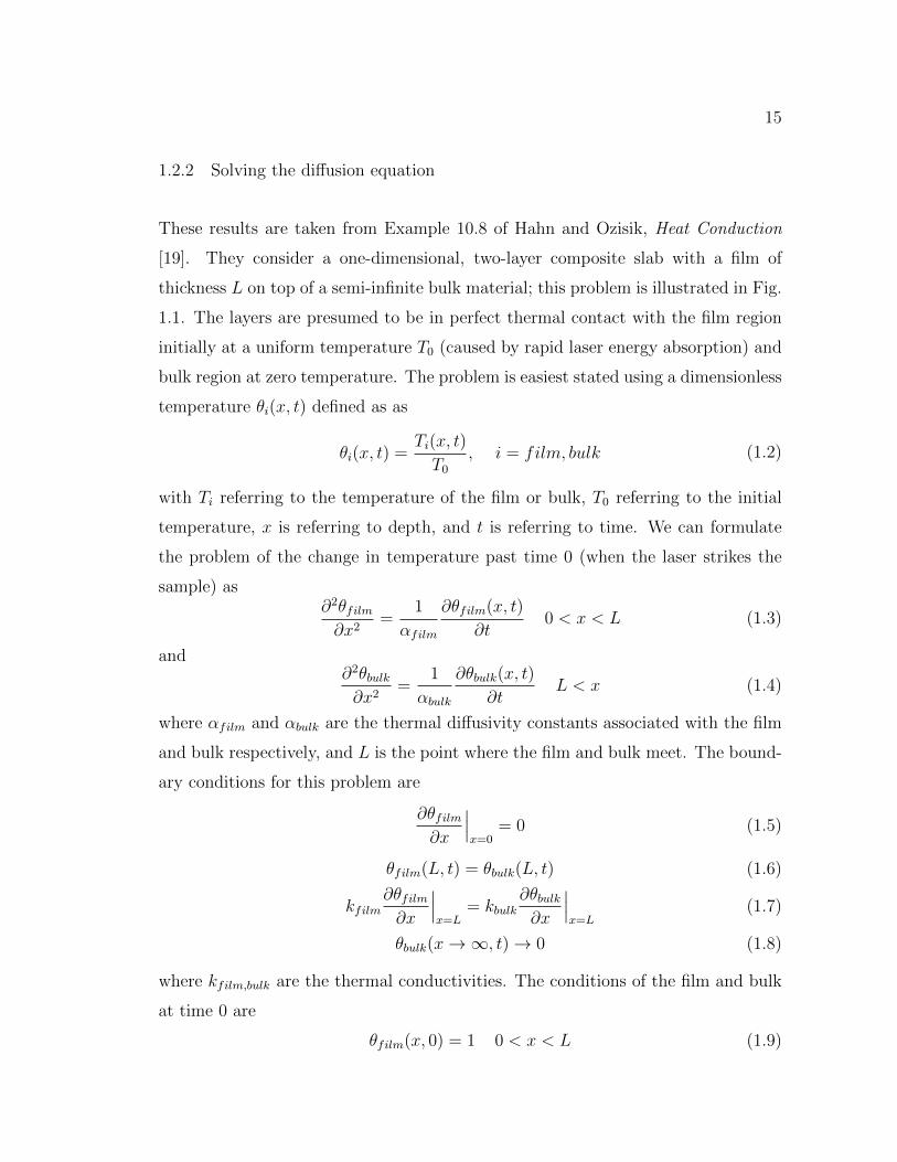
1.2.2 Solving the diffusion equation
These results are taken from Example 10.8 of Hahn and Ozisik, Heat Conduction
[19]. They consider a one-dimensional, two-layer composite slab with a film of
thickness L on top of a semi-infinite bulk material; this problem is illustrated in Fig.
1.1. The layers are presumed to be in perfect thermal contact with the film region
initially at a uniform temperature T0 (caused by rapid laser energy absorption) and
bulk region at zero temperature. The problem is easiest stated using a dimensionless
temperature θi(x, t) defined as as
θi(x, t) =Ti(x, t)
T0
, i = film, bulk (1.2)
with Ti referring to the temperature of the film or bulk, T0 referring to the initial
temperature, x is referring to depth, and t is referring to time. We can formulate
the problem of the change in temperature past time 0 (when the laser strikes the
sample) as∂2θfilm∂x2
=1
αfilm
∂θfilm(x, t)
∂t0 < x < L (1.3)
and∂2θbulk∂x2
=1
αbulk
∂θbulk(x, t)
∂tL < x (1.4)
where αfilm and αbulk are the thermal diffusivity constants associated with the film
and bulk respectively, and L is the point where the film and bulk meet. The bound-
ary conditions for this problem are
∂θfilm∂x
∣∣∣x=0
= 0 (1.5)
θfilm(L, t) = θbulk(L, t) (1.6)
kfilm∂θfilm∂x
∣∣∣x=L
= kbulk∂θbulk∂x
∣∣∣x=L
(1.7)
θbulk(x→∞, t)→ 0 (1.8)
where kfilm,bulk are the thermal conductivities. The conditions of the film and bulk
at time 0 are
θfilm(x, 0) = 1 0 < x < L (1.9)
16
θbulk(x, 0) = 0 L < x (1.10)
At this point, the Laplace transformation is applied both to the model equations and
boundary conditions, to generate ordinary differential equations that can be solved
for the changes in temperature. The resulting equations and boundary conditions
ared2θfilm(x, s)
dx2=
1
αfilm[sθfilm(x, s)− 1] (1.11)
d2θbulk(x, s)
dx2=
1
αbulksθbulk(x, s) (1.12)
dθfilmdx
∣∣∣x=0
= 0 (1.13)
θfilm(L) = θbulk(L) (1.14)
kfilmdθfilmdx
∣∣∣x=L
= kbulkdθbulkdx
∣∣∣x=L
(1.15)
θbulk(x→∞)→ 0 (1.16)
where θi is the Laplace transform of the normalized temperature θ and s is the
Laplace transform of the depth position x. Applying the boundary functions these
resulting equations, the solutions for these ODEs are
θfilm(x, s) =1
s− 1− γ
2s
e−σ(L−x) + e−σ(L+x)
1− γe−2σL0 ≤ x < L (1.17)
θbulk(x, s) =1 + γ
2s
e−σµ(x−L) − e−σ(2L+µx−µL)
1− γe−2σLL < x (1.18)
where
σ ≡√
s
αfilm(1.19)
γ ≡ β − 1
β + 1(1.20)
β ≡ kfilmkbulk
µ. (1.21)
µ =
√αfilmαbulk
(1.22)
The inverse Laplace transform pairs,
17
F (s) F (x)
1s
1
1se−k√x k ≥ 0 erfc( k
2√x)
can now be applied to find the classical model for the temperature profiles,
θfilm(x, t) ≡ 1−1− γ2
∞∑n=0
γn{erfc
[(2n+ 1)L− x
2√αfilmt
]+ erfc
[(2n+ 1)L+ x
2√αfilmt
]}0 < x < L
(1.23)
θbulk(x, t) ≡1 + γ
2
∞∑n=0
γn{erfc
[2nL+ µ(x− L)
2√αfilmt
]− erfc
[(2n+ 2)L+ µ(x− L)
2√αfilmt
]}L < x
(1.24)
where the term [1− γexp(−2σL)] was expanded in a binomial series before perform-
ing the inverse transform.
1.2.3 Example of the classical heat conduction result
To model the experimental results considered in this thesis, the film is set to be 100
nm Cr film directly on top of bulk GaAs. An initial laser fluence of 14.88 mJ/cm2
is used to provide the initial temperature jump in the film,
T0 =F
CfilmLρfilm(1.25)
where F is the absorbed laser fluence, Cfilm is the specific heat of the film, L is the
length of the film, and ρfilm is the mass density of the film. All constants used in
the thermal diffusion calculation are shown in Tables 1.1 and 1.2. Results are shown
in Fig. 1.1. Although only four time points are shown in this figure, the complete
18
thermal profile (to a depth of 10 µm) was calculated at 10,000 depth points for each
of the 753 time points recorded in the experiment, ranging from 30 ps to 3.37 µs .
GaAs Thermal PropertiesQuantity Symbol Value Unit
Mass Density ρbulk 5320 kg/m3
Specific Heat Cbulk 330 J/(kg·K)Thermal Diffusivity αbulk 3.10×10⁻⁵ m2/s
Thermal Conductivity kbulk 55 W/(m·K)
Table 1.1: Values used for calculating thermal transport in the Gallium Arsenidebulk substrate. Note that α = k/ρC.
Cr Thermal PropertiesQuantity Symbol Value UnitThickness L 1×10⁻⁷ m
Mass Density ρfilm 7190 kg/m3
Specific Heat Cfilm 460 J/(kg·K)Thermal Diffusivity αfilm 3.3521×10⁻⁵ m2/s
Thermal Conductivity kfilm 111 W/(m·K)
Table 1.2: Values used for calculating thermal transport in the Cr film.
1.3 Nanoscale thermal transport and the phonon mean free path
Microscopically, heat is transferred by quanta of vibrational energy called phonons.
Phonons are treated using a kinetic model, analogous to the kinetic theory of gasses.
In the kinetic model of gasses, energy is transferred by collisions between individual
gas molecules, which occur on a characteristic collision time that depends on the
density and temperature of the gas. This characteristic collision time can also
be thought of as an average length between collisions, termed the mean free path
(MFP). For a phonon gas, like a gas of molecules, the repeated exchange of energy
following many collisions results eventually in a Maxwell-Boltzmann distribution of
energy at equilibrium, and permits the definition of a temperature. The difference
between these microscopic and macroscopic regimes can be seen in Fig. 1.3
19
Intuitively, heat is transferred faster by phonons that have larger MFPs. The
Maxwell-Boltzmann distribution implies that there is an broad spectrum of phonon
energies at finite temperature. Intuitively, the longer MFP phonons should conduct
heat faster (longer MFPs means heat will travel farther before coming to a stop).
Constraining a new phonon population to have a restricted energy spectrum might
therefore be expected to alter thermal conductivity. In the experiment studied in
this thesis, this restriction of phonon spectrum is accomplished by heating only a
thin metal film, thereby limiting the production of long wavelength (and therefore
low energy and large MFP) phonons, since the film cannot support vibrational modes
(phonons) that are larger than its physical size.
Considerable theoretical efforts have been undertaken to understand how restricting
the available thermal transport channels by limiting phonon spectra alters thermal
conductivity [3]. One example calculation [20] is shown in Fig. 1.2, which shows
longer phonon scattering lengths are required to reach thermal conductivities ap-
proaching bulk values.
To date, none of this depth dependence has been directly observed; the ultimate
goal of this work is to perform temperature depth profile measurements to compare
with those given in Fig. 1.1 and eventually more sophisticated models that can
account for finite size effects, such as the Lattice Boltzmann Model [2].
20
Figure 1.2: A calculation of thermal conductance vs. length, with each curve rep-resenting a different channel length (channel length is the width of the graphenenanoribbon that the phonon MFP travels along). Red circles have a channel lengthof 5 nm, black triangles a channel length of 4 nm, green squares a channel length of3 nm, red triangles a channel length of 2 nm, and blue circles a channel length of 1nm. The dashed line is unit slope. Taken from Aksamija (2017).
21
Figure 1.3: Pictured above are examples of fourier (top) and ballistic heat transport,as we would expect to see in our experimental setup. Notice that in the case offourier heat transport, L is longer than the phonon MFP, whereas L is about thesame length as the phonon MFP is the case of ballistic heat transport.
22
CHAPTER 2
Benchmarking diffraction calculations
2.1 Chapter introduction
The first major project of this thesis was checking a new x-ray diffraction calcula-
tion program (TRXD) against an existing set of tools (GID SL). Tracking thermal
transport throughout a crystal requires making not just a single, high-resolution
recording of an x-ray diffraction pattern, but instead recording an entire sequence
of such patterns. For phenomena such as thermal transport which cover many orders
of magnitude in time (ps to µs), a large number of individual diffraction patterns
must be analyzed in order to stitch together a stop-frame animation of the tempera-
ture profile evolution. This requires a new, efficient, program;TRXD was developed
by DePaul University for this purpose. Here I explain the purpose ofTRXD and
benchmark its results against a standard software package, GID SL.
2.2 X-ray diffraction as a temperature probe
When x-rays of wavelength λ are incident upon a crystal with lattice spacing d,
significant x-ray reflected intensity is found only when the incident angle Θ with
respect to the lattice planes satisfy the condition
nλ = dsin(Θ) (2.1)
where n is the order number of the diffraction peak. This is known as the Bragg Law
of Diffraction. Taking the differential of Bragg’s Law yields a method for measuring
23
small relative changes in lattice spacing ∆d/d, or strain,
∆d
d= −∆Θcot (ΘB) (2.2)
where ∆Θ is a small angular shift away from the Bragg angle ΘB that exactly
satisfies Bragg’s Law. For materials with a linear thermal expansion coefficient αt,
the change in position of a diffraction peaks may be used to calculate a temperature
change ∆T ,
∆T = −∆Θ
αtcot (ΘB) . (2.3)
2.3 Dynamical diffraction
Bragg’s Law is a consequence of Kinematic diffraction theory, which is the appro-
priate method applied when dealing with a small, short range order crystal that
is imperfect. In the kinematic approximation, each cell in the crystal is treated as
being independent, the x-rays are treated as plane waves, and the diffracted electric
field amplitude can be found from
Ediff = EiF∑L
e2πiG·AL , (2.4)
where Ediff is the diffracted wave, Ei is the incident wave, F is the structure vector,
G is the reciprocal lattice vector, A is a unit vector, and L refers to each individual
unit cell. In one dimension, the condition for maximum diffracted electric field
reduces to Bragg’s Law. Within the kinematic approximation, the amplitude of the
diffracted electric field can be decreased as a result of photoelectric absorption.
Calculating diffraction from crystals that are larger and more uniform (or ”perfect”)
requires the use of a more involved theory called dynamical diffraction. Crucially,
dynamical diffraction does not make the assumption that all of the cells in our crystal
are independent. When we use the Darwin-Prins model of dynamical diffraction
[21], there is a range of angles where the reflected intensity is relatively close to the
incident intensity, and the diffraction peaks are no longer delta-functions near ΘB.
24
This relative reflection may be angularly asymmetric. The finite width is due to the
extinction effect, in which dynamical diffraction theory predicts that near strong
reflections, electric field is reduced as energy is reflected outwards rapidly as the
beam penetrates into a material. This results in a reduced number of crystal periods
and limits the exactness with which lattice spacing can be precisely determined
by measurement at one point. Despite this complexity, however, careful analysis
of the diffraction peak lineshape can be used to extract depth-dependent lattice
information, since the diffracted electric field varies throughout the crystal up to
this extinction depth.
2.4 Dynamical diffraction calculations
A standard way of calculating x-ray diffraction peak lineshapes from strained crys-
tals in the dynamical diffraction regime is using the GID SL codes [22, 23]. Unfor-
tunately these are closed-source, server-based programs that do not lend themselves
to solving thousands of diffraction peaks for each sample studied, as required by
time-resolved studies. Furthermore, the ”SL” designation indicates that original
development was for ”superlattices”, or periodic arrangements of strained crystals
that are fabricated, rather than for smooth strain profiles generated by temperature
gradients.
To meet this need, DePaul University began the development of an open-source,
efficient, portable software package namedTRXD that is maintained in a public
depository and is written in the MATLAB programming language [24]. It uses an
alternative algorithm to the one used by GID SL, first described in [15], but with
an adaptive step size in depth that allows the code to handle rapidly changing
strain profiles while retaining computational accuracy. The underlying calculations
are written in matrix form and are vectorized by treating each ∆Θ individually.
Additional computational efficiency is found by using logical array operations to
perform square root operations in the complex plane. An outline of how TRXD
25
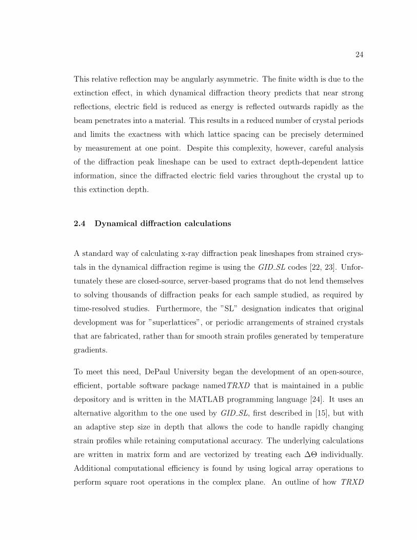
Figure 2.1: Data analysis and modelling procedure. We begin by putting our in-formation into TRXD (timepoints, angular ranges for rocking curve calculations,material constants, and laser fluence), which produces strain profiles that are usedin turn to find the rocking curves expected from the classical model. Next thecentroids are compared to the rocking curve data collected before time zero, whichis used to determine the average temperature change using the thermal expansioncoefficient.
works can be found in Fig. 2.1
2.5 Code benchmarking
Several different comparisons were made between TRXD and GID SL, both for
bulk GaAs with the same reflection order and at the same x-ray energy of 10 keV
used in experiments. The output of each code was formatted as a rocking curve,
or the result that would be obtained as a perfect crystal is slowly rocked along
Θ near the Bragg diffraction peak, while the peak of the total diffracted intensity
was recorded as a function of angle. Benchmarks included unstrained GaAs, or
∆d/d = 0 everywhere, and various uniform strain levels, or ∆d/d = constant. Both
26
codes were run independently, and the results manually imported and overlapped.
No disagreement was found for GaAs at 10 keV, or for the similar semiconductors
Ge, Se, or InSb also used in the larger study at this x-ray energy.
To pull down results from the GID SL server efficiently, a script was written in
MatLAB (see Appendix) that could take an arbitrary depth-dependent strain profile,
such as one generated by the classical thermal diffusion model demonstrated in Fig.
1.1, and break it down into small strain layers for GID SL to calculate. Although
helpful in getting the codes to behave similarly, it proved to be very time-intensive
for the server since a large number of discrete strain points are needed to recapitulate
the smooth strain profile calculated by application of the Fourier Law.
Instead, a different approach was taken: to see if TRXD ’s adaptative step size
technique could handle the abrupt change of a single sharp buried strain level,
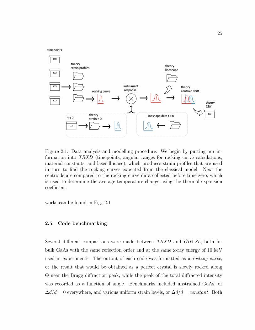
a situation that GID SL was designed to handle. Fig 2.2 shows the result of a
calculation of a strain step-function where ∆d/d = 10−4 over the first 2 µm of the
surface, with the remainder of the bulk crystal unstained. The unstrained rocking
curve is shown for reference, and was identical for both curves. TRXD shows the
overall rocking curve slightly shifted, an effect which is not understood, but which
does not concern us as the shift is small enough to be negligible. The shape however
is otherwise identical. Fig. 2.3 shows the same result, but on a logarithmic intensity
scale.
In addition to quantitative agreement, the results agree with expectations. The
unstrained rocking curve calculation peaks near the calculated Bragg angle of 26.02
degrees, with an intensity just below unity due to a small amount of photoelectric
absorption. The curve is narrow, with an intrinsic width near one millidegree. In
the strained crystal curves, the largest peak is due to the same unstrained substrate,
which is present within the x-ray probe depth of a few microns. This peak is only
slightly distorted, but reduced in intensity. The large secondary peak shifted to
smaller angles corresponds to a positive strain. The peak separation agrees with
27
Figure 2.2: Linear scale comparison ofTRXD and GID SL for a test case of 0.01%uniform strain over the first 2 µm of depth in GaAs [004] reflection at 10 keV. Theunstrained crystal result is shown for reference.
28
Figure 2.3: Linear scale comparison ofTRXD and GID SL for a test case of 0.01%uniform strain over the first 2 µm of depth in GaAs [004] reflection at 10 keV. Theunstrained crystal result is shown for reference.
29
the differential form of Bragg’s Law. Finally, the fringes (more clearly visible in the
logarithmic plot) are due to interferences between the two distinctly strained layers,
with their periodicity given by the strain within our 2 µm depth of our GaAs.
This level of agreement between the new, DePaul-developed TRXD and the widely
used code GID SL demonstrate thatTRXD can be used for analysis of x-ray rocking
curves for the [004] reflection in GaAs at 10 keV.
30
CHAPTER 3
Comparison to experiment
3.1 Chapter introduction
The second major project of this thesis was comparing rocking curves calculated
by the new software TRXD with experimental data. This chapter reviews how the
data was collected, describes the data reduction process, and demonstrates the use
of a Voigt profile to match the angular resolution of experiments with the dynamical
diffraction simulation for comparison.
3.2 Time-resolved x-ray diffraction experiment
Data was collected prior to when I joined the research group by members of Dr.
Landahl’s research group and collaborators, using beamline 7ID of the Advanced
Photon Source at Argonne National Laboratory. Details of the data collection ap-
proach are shown in Fig. 3.1, taken from [14]. Monochromatic 10 keV synchrotron
X-rays (blue) pass through a scattering foil on their way to a sample which is rocked
in small steps across a small angular range near a Bragg peak. The proportional
mode Avalanche Photodiode (APD) collects all x-rays from the diffraction curve,
and has its signal averaged and recorded by an oscilloscope. The x-rays are pro-
duced in 100 ps long bunches separated by 153 ns, and synchronized to an external
50 fs amplified laser pulse (red) that has a pulse repetition frequency of 1 kHz. The
laser triggers the oscilloscope acquisition, which averages for 1000 laser shots before
saving an APD trace. The timing delay between the laser and x-rays can be arbi-
trarily adjusted. The laser also strikes the sample (not shown), focused to ≈ 0.1
31
Figure 3.1: Data collection for time-resolved diffraction measurements used in thisthesis. See the text for full description; taken from Williams (2011).
cm2 to overlap the x-ray spot size of ≈ 50 µm (Vertical) × 500 µm (Horizontal) on
the ≈ 1 cm2 sample. Usually a scattering foil is used to generate a time-resolved
normalization signal by producing a signal that reproduces the uneven fill pattern of
the synchrotron; this typical approach was not used in this data set due to the need
to record very long time-series to follow diffusion process. A different normalization
process using prior bunches with the proportional mode APD was used instead.
32
Figure 3.2: A flowchart picturing how data was extracted (code is attached in theAppendix). From a set of desired time delays, a range of angles covering a rock-ing curve are collected with x-ray bunches both before and after the laser strikesthe sample. Intensities are extracted from oscilloscope traces using SLM and thennormalized using the same x-ray bunch from the preceeding storage ring revolution.These intensities are plotted against the rocking curve angular range to give line-shapes that will be compared to those calculated using a Fourier Law model andTRXD. A compact representation of the data is made by calculating the centroidshift from the rocking curves that we can use to find the average temperature changeof the bulk material region probed by the x-rays.
33
3.3 Data reduction
An outline of this section can be found in Fig. 3.2. Oscilloscope traces were recorded
for 151 angular points, from 27.189 degrees to 27.3090 degrees in 1 millidegree steps
across the Bragg peak (27.2489 degrees at 10 keV) at each time delay. An example
oscilloscope trace is shown in Fig. 3.3. Each x-ray pulse creates a negative voltage
(≈ -35 mV in this case), and overshoots to a positive voltage (≈ +10 mV in this
case) before the next pulse. The synchrotron storage ring was in the standard 24
bunch fill pattern: each 100 ps duration x-ray bunch is separated by 153 ns, with
the total revolution time being 3.68 µs.
On the edges of the rocking curve, the x-ray intensity will be much smaller. Fig.
3.4 shows an oscilloscope pattern at nearly 1000 times smaller x-ray intensity.
Each oscilloscope trace was acquired by averaging for 1,000 laser shots, or one sec-
ond. For each averaged oscilloscope record, 10,000 samples were taken across just
over two storage ring revolutions, which would be 48 bunches in 7.36 µs. This
means there was approximately one sample per nanosecond, or 150 samples per
x-ray bunch. An example of three consecutive x-ray bunches is shown in Fig. 3.5
with each individual oscilloscope sample represented as a point. The x-ray bunches
recorded are much longer than their 100 ps duration, due to the limited bandwidth
of the APD and the oscilloscope.
The Advanced Photon Source synchrotron operates normally in a ”top up” mode
where the individual bunches are routinely filled with more charge to make up for
scattering losses. This refilling is done to maintain average beam current stability,
but results in significant bunch-to-bunch current fluctuations. This is evident in
the oscilloscope trace in Fig. 3.3 which shows considerable variability between each
bunch. This is the purpose of acquiring at least two complete storage ring revolu-
tions: the x-ray intensity in a given bunch does not change in a single revolution,
so the earlier revolution can be used to normalize away these bunch intensity fluc-
34
1 2 3 4 5 6 7 8
Time ( s)
-40
-30
-20
-10
0
10
20
De
tecto
r re
sp
on
se
(m
V)
Figure 3.3: Avalanche Photodiode (APD) detector response to just over two storagering rotations (the data was taken twice - once with and once without the laserheating our sample) in the standard 24 bunch operating mode. This data wasrecorded following diffraction from a laser-excited sample, near the peak of theBragg diffraction peak.
35
0 1 2 3 4 5 6 7 8
Time ( s)
-0.35
-0.3
-0.25
-0.2
-0.15
-0.1
-0.05
De
tecto
r re
sp
on
se
(m
V)
Figure 3.4: APD response from just over two storage ring rotations, but at lowintensity far away from the Bragg diffraction peak.
36
0 100 200 300 400 500
Time (ns)
-40
-30
-20
-10
0
10
20
De
tecto
r re
sp
on
se
(m
V)
Figure 3.5: APD response from only 3 bunches, showing individual oscilloscopesamples as points. Approximately one sample is taken every nanosecond, with 153ns between x-ray bunches in the standard 24 bunch mode of the APS.
37
0 0.5 1 1.5 2 2.5 3 3.5
Time ( s)
-40
-30
-20
-10
0
10
20D
ete
cto
r re
sp
on
se
(m
V)
Figure 3.6: APD response from two consecutive storage ring rotations overlapped.The later revolution is shown in red, the earlier pre-laser revolution is in blue. Thelaser strikes the sample, altering x-ray diffraction intensity just before the fourthbunch. Thermal recovery is observed over several µs as the red and blue curvesapproach each other.
tuations. This is illustrated in Fig. 3.6 which shows the exact sample oscilloscope
trace as Fig. 3.3, but with the second set of 24 bunches translated earlier in time
by one ring revolution. The earlier bunches are in blue and the later bunches are
superimposed in red. Although the total pattern looks noisy, in fact the first 3
bunches are seen to overlap nearly perfectly. The laser strikes the sample after the
third bunch, and so the remaining bunches see a difference in x-ray intensity. It is
this comparison method that allows for very small changes in x-ray intensity, and
therefore very small changes in x-ray rocking curve position (and therefore Bragg
angle shift and ultimately temperature changes) to be recorded.
38
The next data reduction step is extracting an x-ray intensity from the trace of each
bunch. The APD pulses are created by charges generated by the absorption of x-rays
in the detector, which is then amplified via both internal processes (avalanching)
and external electronic high-speed amplifiers. Therefore, with a fixed time response,
either measuring the pulse height or area under each curve should give a measure-
ment of x-ray intensity. The changing overshoot (recovery) of the proportional mode
detector makes this difficult. Therefore the research group has been developing a
new analysis method based on Shape Language Modeling (SLM), demonstrated in
Figs. 3.7-3.10. Note that the inverse of the raw data shown previously has been
taken in these plots for clarity (so that each x-ray bunch now goes up with intensity).
SLM uses constrained piecewise continuous cubic spline interpolation to model ar-
bitrarily shaped data, and is available as a MatLAB package [25]. As shown in Fig.
3.7 for higher x-ray intensity data samples (blue circles), ”knot” locations (vertical
green dashed lines) are chosen as fixed locations where the cubic splines are joined.
Additional constraints are applied in this SLM, such as requiring monotonic rising
behavior before the peak and falling behavior following the peak. The SLM curve
(red line) therefore provides an appropriately smoothed empirical fit to the data,
allowing the minimum and maximum peak height to be extracted while using the
entire sample set across the peak.
The utility of this approach is demonstrated in Fig. 3.8, which is from an x-ray
bunch recorded at a lower intensity region of the rocking curve. Selecting just the
minimum and maximum of the data in this region is sensitive to noise at these low
signal levels, and subtracting the extrema would result in an overestimate of x-ray
intensity. Fig. 3.9 shows the ability of SLM to extract x-ray intensities that are
only 40 µV in height, implying that a dynamic range of over 3 orders of magnitude
can be obtained in this time-resolved measurement when compared with Fig. 3.7.
Finally, Fig. 3.10 shows that the SLM data extraction method can begin to fail
when the intensity gets low enough, with the x-ray intensity likely over-estimating
differences between a peak and signal that may not actually exist.
39
0 50 100 150 200
Sample Number
-20
-10
0
10
20
30
40
AP
D R
esp
op
nse
(m
V)
Figure 3.7: Fitting the inverted APD response (blue points) to a single x-ray bunchat relatively high x-ray intensity using SLM (red line). Knot locations where cubicsplines are tied together are shown as dashed green lines.
40
0 50 100 150 200
Sample Number
0.12
0.14
0.16
0.18
0.2
0.22
0.24
AP
D R
esp
op
nse
(m
V)
Figure 3.8: Fitting a the inverted APD response (blue points) to a single x-raybunch at relatively low x-ray intensity using SLM (red line). Knot locations are thegreen dashed lines.
41
0 50 100 150 200
Sample Number
0.12
0.13
0.14
0.15
0.16
0.17
0.18
0.19
0.2
0.21
AP
D R
esp
op
nse
(m
V)
Figure 3.9: Fitting the inverted APD response (blue points) to a single x-ray bunchat very low x-ray intensity using SLM (red line). Knot locations are the green dashedlines. High noise levels would cause overestimation of extrema difference withoutSLM-assisted data smoothing.
42
0 50 100 150 200
Sample Number
0.12
0.13
0.14
0.15
0.16
0.17
0.18
0.19
0.2
AP
D R
esp
op
nse
(m
V)
Figure 3.10: Fitting the inverted APD response (blue points) to a single x-ray bunchat vanishingly low x-ray intensity using SLM (red line). Knot locations are the greendashed lines. SLM likely causes overestimation of a signal that is buried in noise.
43
3.4 Convolution with instrument resolution
The dynamical diffraction peak shapes calculated using either TRXD or GID SL
represent an ideal experimental situation where the incident x-ray beam has no
energy spread or angular spread, and the unstrained GaAs substrate is truly perfect.
All of these effects add blurring to the rocking curves. To account for the loss
in resolution, each calculated rocking curve is convolved with a normalized Voigt
profile,
Imeas(Θ) =
∫ ∞−∞
V (Θ′)Icalc(Θ−Θ′)dΘ′ + I0 (3.1)
where Icalc(Θ) is the calculated rocking curve intensity from TRXD, I0 is a constant
offset to compensate for the overestimation of extremely small signals due to SLM
as described in Fig. 3.10, and Imeas(Θ) is the anticipated measured rocking curve
following convolution with the instrument response function described as a Voigt
curve V ,
V (Θ) =
∫ ∞−∞
G(Θ′)L(Θ−Θ′)dΘ′ (3.2)
which is itself a convolution of a Lorentzian lineshape,
L(Θ) =γ
π (Θ2 + γ2)(3.3)
with a Gaussian lineshape,
G(Θ) =e−Θ2/(2σ2)
σ√
2π. (3.4)
The Lorentzian width, γ, Gaussian width, σ, and fixed offset, I0 are all free parame-
ters chosen to overlap the calculations for unstrained data with the measurement of
the unstrained crystal sample, taken from the x-ray bunch before the laser strikes the
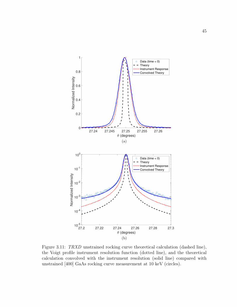
sample, i.e. when t < 0. The success of the Voigt profile in matching the experiment
to the data is shown in Fig. 3.11, and is subsequently applied to all other strained
rocking curves, prior to intensity normalization. A best fit to data was found with
γ = 0.35 mdeg, σ = 1.45 mdeg, and I0 = 0.5% of the maximum intensity. These
are reasonable values given that the angular step size taken in the experiment was
44
only 1.0 mdeg, corresponding to the smallest angular step size that could be repeat-
ably performed by the diffraction instrument. A function for efficiently convolving
rocking curves with this instrument response is included in the Appendix. Future
work may include modifying the Voigt profile with an asymmetric Lorentzian profile
to better match the data. The success of TRXD in modeling unstrained x-ray
diffraction data for this experiment indicates that study of thermal transport using
the same data reduction and instrument resolution methods should be valid.
45
27.24 27.245 27.25 27.255 27.26
(degrees)
0
0.2
0.4
0.6
0.8
1
No
rma
lize
d I
nte
nsity
Data (time < 0)
Theory
Instrument Response
Convolved Theory
(a)
27.2 27.22 27.24 27.26 27.28 27.3
(degrees)
10-5
10-4
10-3
10-2
10-1
100
No
rma
lize
d I
nte
nsity
Data (time < 0)
Theory
Instrument Response
Convolved Theory
(b)
Figure 3.11: TRXD unstrained rocking curve theoretical calculation (dashed line),the Voigt profile instrument resolution function (dotted line), and the theoreticalcalculation convolved with the instrument resolution (solid line) compared withunstrained [400] GaAs rocking curve measurement at 10 keV (circles).
46
CHAPTER 4
Agreement and discrepancy with classical theory
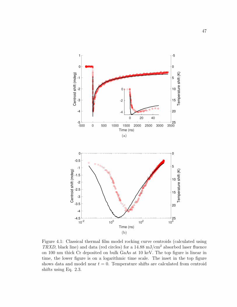
The centroid of the diffraction peaks at each measured time delay was determined
for both the classical thermal film model and the data, and subtracted from the
measured centroid of the unstrained crystal (Bragg diffraction peak). A single free
parameter, the absorbed laser fluence, was adjusted to match experiment
with data. The results of the calculation are shown overlapped with the data in
Fig 4.1. Data is collected before the laser strikes the sample (when t < 0) as a
control, and is found to have zero shift from the unstrained measurements.
The behavior seen in Fig. 4.1 can mostly, but not entirely be explained by the
classical thermal film model of Eq. 1.24. The first few tens of ps cannot be accurately
observed, due to the x-ray bunch duration of 100 ps which would blur out the earliest
and fastest movement of heat into the substrate. Although the temperature at the
film/substrate interface is initially very high, as seen at 1 ns in Fig. 1.1, it has
not diffused very far into the substrate and therefore only a small fraction of the x-
rays within the penetration depth experience a diffraction peak shift, so the average
centroid shift at first is small. This increases rapidly as the heat continues to flow
into the x-ray probe depth, shifting the peak to lower angles in agreement with Eq.
2.3. After about 10 ns, the peak average lattice expansion is reached as the heat
begins to flow out of the x-ray probe depth, and the surface of the crystal begins
to slowly cool. The first several microns of the substrate have nearly reached the
original temperature by 3.5 µs, when data collection ends. The crystal will have
completely recovered before the next laser pulse re-heats the sample in 1 ms.
The theoretical curves show a very similar cooling rate past 100 ns. The small differ-
47
-500 0 500 1000 1500 2000 2500 3000 3500
Time (ns)
-5
-4
-3
-2
-1
0
1
Ce
ntr
oid
sh
ift
(md
eg
)
-5
0
5
10
15
20
25
Te
mp
era
ture
sh
ift
(K)
0 20 40
-4
-2
0
(a)
10-2
100
102
104
Time (ns)
-4.5
-4
-3.5
-3
-2.5
-2
-1.5
-1
-0.5
0
Ce
ntr
oid
sh
ift
(md
eg
)
0
5
10
15
20
25
Te
mp
era
ture
sh
ift
(K)
(b)
Figure 4.1: Classical thermal film model rocking curve centroids (calculated usingTRXD, black line) and data (red circles) for a 14.88 mJ/cm2 absorbed laser fluenceon 100 nm thick Cr deposited on bulk GaAs at 10 keV. The top figure is linear intime, the lower figure is on a logarithmic time scale. The inset in the top figureshows data and model near t = 0. Temperature shifts are calculated from centroidshifts using Eq. 2.3.
48
ences observed may be due to the neglect of other thermal dissipation mechanisms
not included in the model, such as lateral heat conduction (only a 1D model is
used), or radiative heat off the surface. Unsurprisingly, the classical Fourier Law of
heat transfer is found to qualitatively and quantitatively describe the data at long
timescales, or when the heat has already spread over a macroscopic distance. The
values of thermal conductivity for GaAs are well established, and this measurement
is in agreement.
There is significant disagreement however at times below 100 ns. First, in order
to match the long-timescale cooling, the maximum laser fluence had to be raised
about 20% over value needed to reach the peak lattice displacement observed. This
is most clear in the logarithmic time (lower) plot in Fig. 4.1, which shows a measured
maximum negative centroid shift of -4 mdeg, but a corresponding simulation value
of -4.5 mdeg. Second, the maximum angular shift occurs significantly earlier for the
model than for the data. This is also clear from the inset in the upper figure, which
shows a difference of close to 10 ns between theory and experiment.
This data, along with confidence in the TRXD simulation tool gained
from the earlier chapters of this thesis, provides clear evidence for the
central hypothesis of nanoscale thermal transport described in the first
chapter: that heat conducts slower at short distances than in bulk materi-
als. It takes longer to transmit from the 100 nm thick Cr film into the substrate than
would be expected by classical theory, but after a few ns it behaves as predicted by
Fourier the half-millimeter thick GaAs substrate. This observation confirms quanti-
tatively the one made by the research group in 2007. Their main result is duplicated
in Fig. 4.2 [11].
Notably, the heat impulses also arrive later in the data than in the simulation for
the 2007 result, and also require a similarly higher laser fluence to match the peak
position. This is remarkable given that the entire rocking curve shape was estimated
from a single data point taken at the half-maximum of the diffraction curve, and
49
Figure 4.2: Previously published results by Highland et al., 2007 using time-resolvedx-ray diffraction to study a 100 nm metallic film on GaAs. The figure shows thetime evolution of the average temperature of layer as determined from shifts of thediffraction peak, see Eq. (12) of Highland. The dashed lines are the evolution ofthe weighted average temperature of the buried layer predicted by a solution to thediffusion equation using the values of probe layers fabricated from InGaAs alloys of246 nm, 161 nm, and 126 nm on top of the GaAs substrate but below the film. Dotsare data, not from centroids, but deduced from a single data point located at thehalf-maximum of the rocking curve. Dashed lines are a classical thermal transportmodel, and the solid line was a two-channel model developed to describe the dataset.
50
that dynamical diffraction theory was not used in the interpretation of the result –
only three separate depth probe heights were used at 246 nm, 161 nm, and 126 nm
below the film. Our results, analyzed with TRXD, are in strong agreement
with this earlier published data and show similar discrepancies with the
Fourier Law.
Dynamical diffraction measurements and calculations however can tell a great deal
more about exactly what happens to the missing heat, which could only be guessed
at in Highland et al.. In that paper, the slowed cooling was attributed to a second
thermal transit channel, containing about 20% of the total thermal energy, and
resulting from ”ballistic” phonon transport, i.e. transport events within a phonon
MFP.
Now, however, we are able to see exactly what the diffraction patterns are at each
measured timepoint, and compare them with a model that uses a benchmarked
dynamical diffraction code to compare them with the detailed result of the classical
simulation. A selection of representative high resolution rocking curve calculations
and measurements are presented in Figs. 4.3 - 4.14 and are discussed in the next
section.
4.1 Observed behavior
The first frame recorded after the laser strikes the sample, shown in Fig. 4.3,
shows only a slight change in x-ray reflectivity that is primarily in the wings of the
diffraction peak. Substantial changes in the diffraction peak shape appear within
the first nanosecond, e.g. Fig. ??. According to the Fourier Law model, the
heat should diffuse into the sample a characteristic diffusion length of LD =√
4αt.
Using the value of the diffusivity, α, from 1.1, the temperature jump should have
travelled 350 nm in the first 1 ns. This is also demonstrated in the calculated
temperature profile shown in Fig.1.24 as the red curve. However the x-rays are
51
27.24 27.245 27.25 27.255
(degrees)
0
0.2
0.4
0.6
0.8
1
Norm
aliz
ed Inte
nsity
0.0 ns
(a)
27.2 27.22 27.24 27.26 27.28 27.3
(degrees)
10-4
10-3
10-2
10-1
100
No
rma
lize
d I
nte
nsity
0.0 ns
(b)
Figure 4.3: t = 0 ns diffraction data (red filled circles), classical thermal transportsimulation (red line), and t < 0 data (open blue circles) and simulation (blue line).t = 0 ns or “time zero” is the earliest data point where a significant difference isseen in the x-ray data from the proceeding x-ray bunch.
52
27.24 27.245 27.25 27.255
(degrees)
0
0.2
0.4
0.6
0.8
1
No
rma
lize
d I
nte
nsity
0.5 ns
(a)
27.2 27.22 27.24 27.26 27.28 27.3
(degrees)
10-4
10-3
10-2
10-1
100
No
rma
lize
d I
nte
nsity
0.5 ns
(b)
Figure 4.4: t = 0.5 ns diffraction data (red filled circles), classical thermal transportsimulation (red line), and t < 0 data (open blue circles) and simulation (blue line).The x-ray data (which is entirely dependent upon the substrate) shows significantfringes which cannot be explained by the Fourier Law.
53
27.24 27.245 27.25 27.255
(degrees)
0
0.2
0.4
0.6
0.8
1
No
rma
lize
d I
nte
nsity
1.0 ns
(a)
27.2 27.22 27.24 27.26 27.28 27.3
(degrees)
10-4
10-3
10-2
10-1
100
No
rma
lize
d I
nte
nsity
1.0 ns
(b)
Figure 4.5: t = 1.0 ns diffraction data (red filled circles), classical thermal transportsimulation (red line), and t < 0 data (open blue circles) and simulation (blue line).Both simulation and data peaks show a shifting and broadening, consistent witha non-uniform temperature gradient as the heat is just beginning to flow into thesubstrate. The Fourier Law simulation shows a greater average temperature thanthe data.
54
27.24 27.245 27.25 27.255
(degrees)
0
0.2
0.4
0.6
0.8
1
No
rma
lize
d I
nte
nsity
5.4 ns
(a)
27.2 27.22 27.24 27.26 27.28 27.3
(degrees)
10-4
10-3
10-2
10-1
100
No
rma
lize
d I
nte
nsity
5.4 ns
(b)
Figure 4.6: t = 5.4 ns diffraction data (red filled circles), classical thermal transportsimulation (red line), and t < 0 data (open blue circles) and simulation (blue line).This is near the maximum centroid shift predicted by the Fourier simulation.
55
27.24 27.245 27.25 27.255
(degrees)
0
0.2
0.4
0.6
0.8
1
No
rma
lize
d I
nte
nsity
10.4 ns
(a)
27.2 27.22 27.24 27.26 27.28 27.3
(degrees)
10-4
10-3
10-2
10-1
100
No
rma
lize
d I
nte
nsity
10.4 ns
(b)
Figure 4.7: t = 10.4 ns diffraction data (red filled circles), classical thermal transportsimulation (red line), and t < 0 data (open blue circles) and simulation (blue line).This is near the maximum centroid shift measured, but after the maximum shiftfound in the simulation.
56
27.24 27.245 27.25 27.255
(degrees)
0
0.2
0.4
0.6
0.8
1
No
rma
lize
d I
nte
nsity
25.4 ns
(a)
27.2 27.22 27.24 27.26 27.28 27.3
(degrees)
10-4
10-3
10-2
10-1
100
No
rma
lize
d I
nte
nsity
25.4 ns
(b)
Figure 4.8: t = 25.4 ns diffraction data (red filled circles), classical thermal trans-port simulation (red line), and t < 0 data (open blue circles) and simulation (blueline). This is past the point of maximum peak shift for both the simulation andmeasurement, and just as cooling is starting.
57
27.24 27.245 27.25 27.255
(degrees)
0
0.2
0.4
0.6
0.8
1
No
rma
lize
d I
nte
nsity
48.8 ns
(a)
27.2 27.22 27.24 27.26 27.28 27.3
(degrees)
10-4
10-3
10-2
10-1
100
No
rma
lize
d I
nte
nsity
48.8 ns
(b)
Figure 4.9: t = 48.8 ns diffraction data (red filled circles), classical thermal trans-port simulation (red line), and t < 0 data (open blue circles) and simulation (blueline). The calculated and measured peaks are beginning to narrow, indicating thattemperature is becoming more homogenous throughout the substrate surface.
58
27.24 27.245 27.25 27.255
(degrees)
0
0.2
0.4
0.6
0.8
1
No
rma
lize
d I
nte
nsity
98.8 ns
(a)
27.2 27.22 27.24 27.26 27.28 27.3
(degrees)
10-4
10-3
10-2
10-1
100
No
rma
lize
d I
nte
nsity
98.8 ns
(b)
Figure 4.10: t = 98.8 ns diffraction data (red filled circles), classical thermal trans-port simulation (red line), and t < 0 data (open blue circles) and simulation (blueline). Cooling continues as the centroid shift reduces.
59
27.24 27.245 27.25 27.255
(degrees)
0
0.2
0.4
0.6
0.8
1
No
rma
lize
d I
nte
nsity
252.2 ns
(a)
27.2 27.22 27.24 27.26 27.28 27.3
(degrees)
10-4
10-3
10-2
10-1
100
No
rma
lize
d I
nte
nsity
252.2 ns
(b)
Figure 4.11: t = 252.2 ns diffraction data (red filled circles), classical thermal trans-port simulation (red line), and t < 0 data (open blue circles) and simulation (blueline). The strained and unstrained rocking curves now have similar shapes andwidths, indicating that the probed length the substrate is at a uniform, but stillelevated temperature.
60
27.24 27.245 27.25 27.255
(degrees)
0
0.2
0.4
0.6
0.8
1
No
rma
lize
d I
nte
nsity
498.9 ns
(a)
27.2 27.22 27.24 27.26 27.28 27.3
(degrees)
10-4
10-3
10-2
10-1
100
No
rma
lize
d I
nte
nsity
498.9 ns
(b)
Figure 4.12: t = 498.9 ns diffraction data (red filled circles), classical thermal trans-port simulation (red line), and t < 0 data (open blue circles) and simulation (blueline). Agreement between the Fourier theory and measurement is now very close.
61
27.24 27.245 27.25 27.255
(degrees)
0
0.2
0.4
0.6
0.8
1
No
rma
lize
d I
nte
nsity
1499.1 ns
(a)
27.2 27.22 27.24 27.26 27.28 27.3
(degrees)
10-4
10-3
10-2
10-1
100
No
rma
lize
d I
nte
nsity
1499.1 ns
(b)
Figure 4.13: t = 1499.1 ns diffraction data (red filled circles), classical thermaltransport simulation (red line), and t < 0 data (open blue circles) and simulation(blue line). The temperature difference is now a uniform 5 degrees C.
62
27.24 27.245 27.25 27.255
(degrees)
0
0.2
0.4
0.6
0.8
1
No
rma
lize
d I
nte
nsity
3249.4 ns
(a)
27.2 27.22 27.24 27.26 27.28 27.3
(degrees)
10-4
10-3
10-2
10-1
100
No
rma
lize
d I
nte
nsity
3249.4 ns
(b)
Figure 4.14: t = 3249.4 ns diffraction data (red filled circles), classical thermaltransport simulation (red line), and t < 0 data (open blue circles) and simulation(blue line). By the latest timepoints recorded, the agreement between the FourierTheory and measurement is almost as good as for the unstrained rocking curves.The strain is completely uniform throughout the probed crystal depth.
63
probing an extinction depth of over 2000 nm, meaning that only one fifth of probed
volume is strained. Therefore, the Fourier Law would predict a strong double-peaked
curve, corresponding two a thin strained layer near the surface and then the larger
underlying bulk volume which remains unaffected at these times. When these early
strain profiles are converted into diffraction peak shapes by TRXD, they do indeed
show a double-peak which slowly merges with the main peak as time continues. By
25 ns, the Fourier Law predicts a single, significantly broadened peak as the strain
continuously decreases all the way out to the x-ray extinction depth of 1.7 µm. This
is seen in the simulation curves of Figs. 4.4 - 4.8.
However, the actual measured diffraction peaks completely disagree with calculation,
indicating the the Fourier Law does not properly predict the shape of the temper-
ature profile at t < 25 ns. Instead, the data initially shows symmetric fringes, im-
plying both an expansion and a compression of GaAs. This previously undiscovered
behavior is discussed in the next chapter. Given the disagreement about diffraction
peak shape, it is no surprise that the calculated centroid peak shifts and average
temperature of the GaAs as seen in Fig. 4.1 also disagrees with measurement at
these times.
Once the heat impulse has travelled throughout the probe depth, we see that the
Fourier Law begins to behave more qualitatively like the abservations. The merged,
broadened peak begins to narrow beginning at 100 ns (Fig. 4.10) as the strain profiles
become uniform over the entire probed volume. By 1500 ns the laser-excited crystal
has the same diffraction peak width as the initially unstrained crystal (Fig. 4.13,
indicating a uniform but elevated tempearture that is also in quantitative agreement
with the Fourier Law prediction. The experiment is now well within the regime of
Fourier Law validity, as cooling of the probed volume continues via classical thermal
diffusion as the heat flows into the unmeasured crystal bulk (Fig. 4.14. The crystal
wafer is 500 µm thick, implying that it would take over 1 ms for heat to reach the
rear side of the wafer. By this time, the next pulse of the 1 kHz repetition rate laser
has hit the front surface with the metallic film, repeating the experiment.
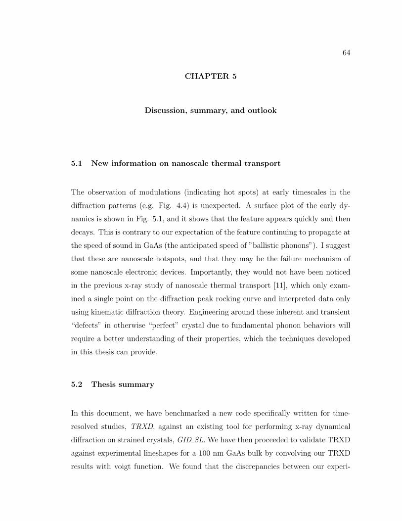
64
CHAPTER 5
Discussion, summary, and outlook
5.1 New information on nanoscale thermal transport
The observation of modulations (indicating hot spots) at early timescales in the
diffraction patterns (e.g. Fig. 4.4) is unexpected. A surface plot of the early dy-
namics is shown in Fig. 5.1, and it shows that the feature appears quickly and then
decays. This is contrary to our expectation of the feature continuing to propagate at
the speed of sound in GaAs (the anticipated speed of ”ballistic phonons”). I suggest
that these are nanoscale hotspots, and that they may be the failure mechanism of
some nanoscale electronic devices. Importantly, they would not have been noticed
in the previous x-ray study of nanoscale thermal transport [11], which only exam-
ined a single point on the diffraction peak rocking curve and interpreted data only
using kinematic diffraction theory. Engineering around these inherent and transient
“defects” in otherwise “perfect” crystal due to fundamental phonon behaviors will
require a better understanding of their properties, which the techniques developed
in this thesis can provide.
5.2 Thesis summary
In this document, we have benchmarked a new code specifically written for time-
resolved studies, TRXD, against an existing tool for performing x-ray dynamical
diffraction on strained crystals, GID SL. We have then proceeded to validate TRXD
against experimental lineshapes for a 100 nm GaAs bulk by convolving our TRXD
results with voigt function. We found that the discrepancies between our experi-
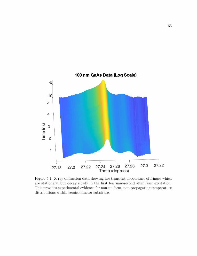
65
Figure 5.1: X-ray diffraction data showing the transient appearance of fringes whichare stationary, but decay slowly in the first few nanosecond after laser excitation.This provides experimental evidence for non-uniform, non-propagating temperaturedistributions within semiconductor substrate.
66
mental results and Fourier Theory matched those of earlier work, suggesting heat
transfers slower at short times and distances. Additionally, the data set we used
contains the first structural data showing the appearance of non-uniform strain in
a previously uniform crystal due to nanoscale thermal transport.
5.3 Outlook
Going forward, there are several ways this research can be improved or expanded
upon. First, the data set used contains experimental data for lineshapes other
than our 100 nm GaAs bulk with chromium film - TRXD should be tested against
this additional data. This includes 100 nm, 200 nm, and 400 nm Cr films on not
just GaAs, but also the bulk semiconductor materials InSb, Ge, and Si. Next,
general methods for inverting dynamical diffraction data to calculate strain profiles
(and therefore temperature profiles) should be implemented using TRXD, e.g. [16]
and [17]. Additionally, the most recent theoretical models for nanoscale thermal
transport, e.g. Lattice Boltzmann Models [2], should be tested against these new
validated data sets and diffraction calculations. Finally, we will seek to determine
the exact temperature depth profile and extract the phonon mean free path spectra
directly from structure.
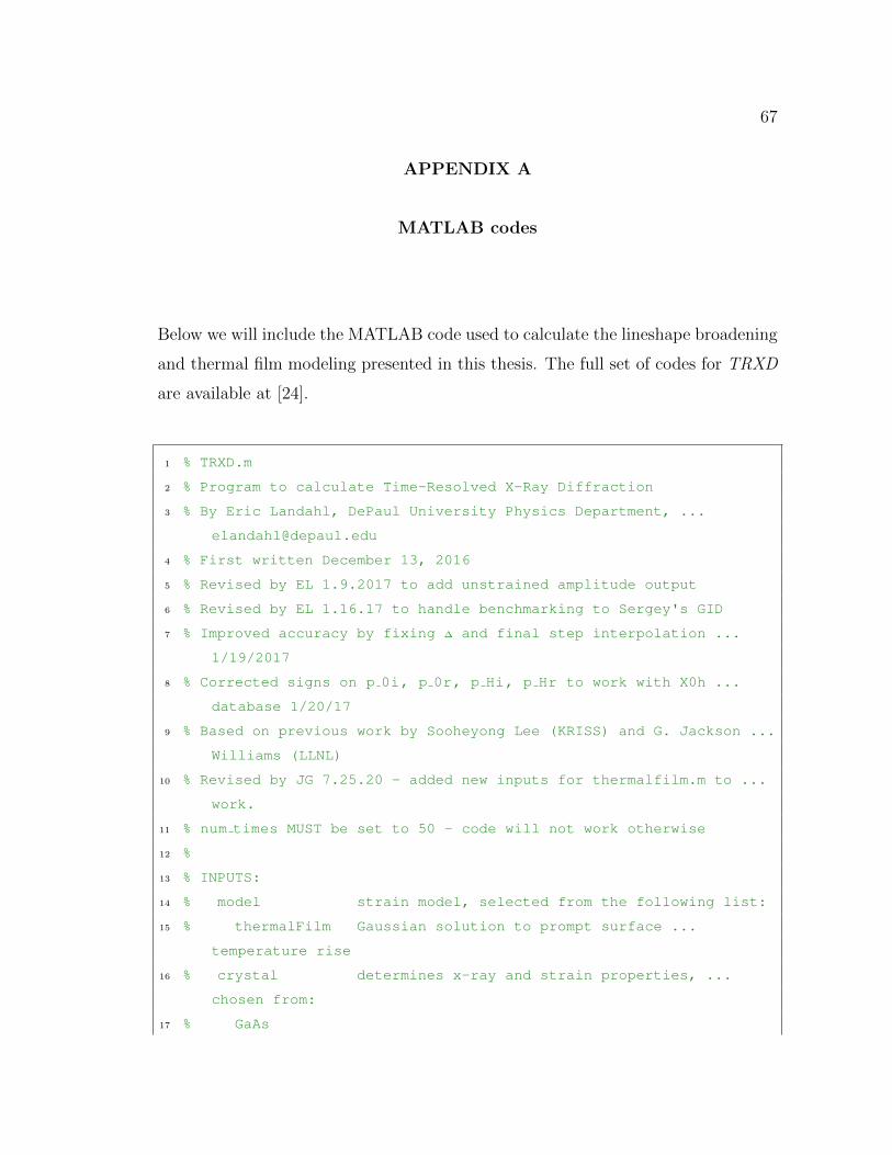
67
APPENDIX A
MATLAB codes
Below we will include the MATLAB code used to calculate the lineshape broadening
and thermal film modeling presented in this thesis. The full set of codes for TRXD
are available at [24].
1 % TRXD.m
2 % Program to calculate Time-Resolved X-Ray Diffraction
3 % By Eric Landahl, DePaul University Physics Department, ...
4 % First written December 13, 2016
5 % Revised by EL 1.9.2017 to add unstrained amplitude output
6 % Revised by EL 1.16.17 to handle benchmarking to Sergey's GID
7 % Improved accuracy by fixing ∆ and final step interpolation ...
1/19/2017
8 % Corrected signs on p 0i, p 0r, p Hi, p Hr to work with X0h ...
database 1/20/17
9 % Based on previous work by Sooheyong Lee (KRISS) and G. Jackson ...
Williams (LLNL)
10 % Revised by JG 7.25.20 - added new inputs for thermalfilm.m to ...
work.
11 % num times MUST be set to 50 - code will not work otherwise
12 %
13 % INPUTS:
14 % model strain model, selected from the following list:
15 % thermalFilm Gaussian solution to prompt surface ...
temperature rise
16 % crystal determines x-ray and strain properties, ...
chosen from:
17 % GaAs
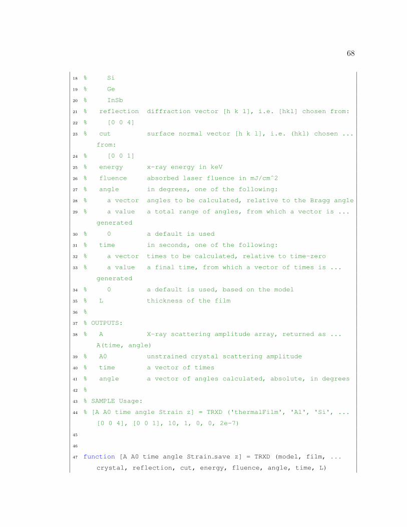
68
18 % Si
19 % Ge
20 % InSb
21 % reflection diffraction vector [h k l], i.e. [hkl] chosen from:
22 % [0 0 4]
23 % cut surface normal vector [h k l], i.e. (hkl) chosen ...
from:
24 % [0 0 1]
25 % energy x-ray energy in keV
26 % fluence absorbed laser fluence in mJ/cmˆ2
27 % angle in degrees, one of the following:
28 % a vector angles to be calculated, relative to the Bragg angle
29 % a value a total range of angles, from which a vector is ...
generated
30 % 0 a default is used
31 % time in seconds, one of the following:
32 % a vector times to be calculated, relative to time-zero
33 % a value a final time, from which a vector of times is ...
generated
34 % 0 a default is used, based on the model
35 % L thickness of the film
36 %
37 % OUTPUTS:
38 % A X-ray scattering amplitude array, returned as ...
A(time, angle)
39 % A0 unstrained crystal scattering amplitude
40 % time a vector of times
41 % angle a vector of angles calculated, absolute, in degrees
42 %
43 % SAMPLE Usage:
44 % [A A0 time angle Strain z] = TRXD ('thermalFilm', 'Al', 'Si', ...
[0 0 4], [0 0 1], 10, 1, 0, 0, 2e-7)
45
46
47 function [A A0 time angle Strain save z] = TRXD (model, film, ...
crystal, reflection, cut, energy, fluence, angle, time, L)
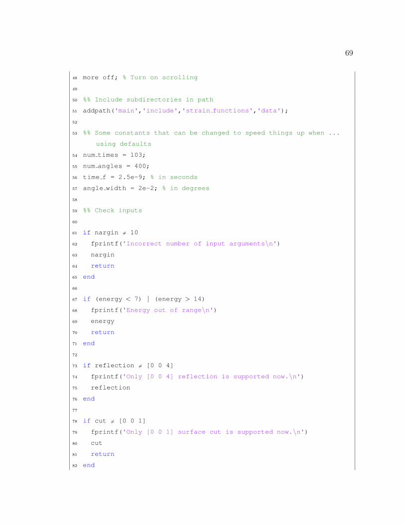
69
48 more off; % Turn on scrolling
49
50 %% Include subdirectories in path
51 addpath('main','include','strain functions','data');
52
53 %% Some constants that can be changed to speed things up when ...
using defaults
54 num times = 103;
55 num angles = 400;
56 time f = 2.5e-9; % in seconds
57 angle width = 2e-2; % in degrees
58
59 %% Check inputs
60
61 if nargin 6= 10
62 fprintf('Incorrect number of input arguments\n')63 nargin
64 return
65 end
66
67 if (energy < 7) | (energy > 14)
68 fprintf('Energy out of range\n')69 energy
70 return
71 end
72
73 if reflection 6= [0 0 4]
74 fprintf('Only [0 0 4] reflection is supported now.\n')75 reflection
76 end
77
78 if cut 6= [0 0 1]
79 fprintf('Only [0 0 1] surface cut is supported now.\n')80 cut
81 return
82 end
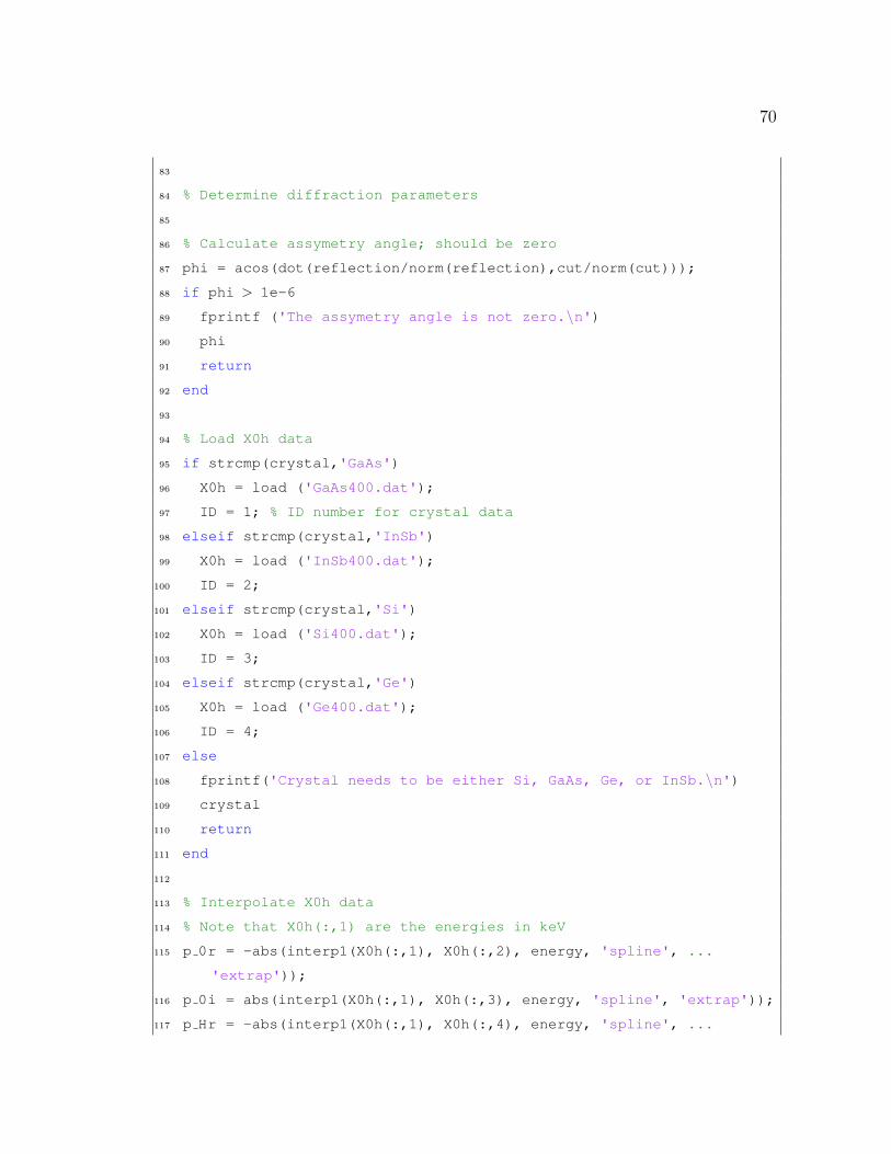
70
83
84 % Determine diffraction parameters
85
86 % Calculate assymetry angle; should be zero
87 phi = acos(dot(reflection/norm(reflection),cut/norm(cut)));
88 if phi > 1e-6
89 fprintf ('The assymetry angle is not zero.\n')90 phi
91 return
92 end
93
94 % Load X0h data
95 if strcmp(crystal,'GaAs')
96 X0h = load ('GaAs400.dat');
97 ID = 1; % ID number for crystal data
98 elseif strcmp(crystal,'InSb')
99 X0h = load ('InSb400.dat');
100 ID = 2;
101 elseif strcmp(crystal,'Si')
102 X0h = load ('Si400.dat');
103 ID = 3;
104 elseif strcmp(crystal,'Ge')
105 X0h = load ('Ge400.dat');
106 ID = 4;
107 else
108 fprintf('Crystal needs to be either Si, GaAs, Ge, or InSb.\n')109 crystal
110 return
111 end
112
113 % Interpolate X0h data
114 % Note that X0h(:,1) are the energies in keV
115 p 0r = -abs(interp1(X0h(:,1), X0h(:,2), energy, 'spline', ...
'extrap'));
116 p 0i = abs(interp1(X0h(:,1), X0h(:,3), energy, 'spline', 'extrap'));
117 p Hr = -abs(interp1(X0h(:,1), X0h(:,4), energy, 'spline', ...
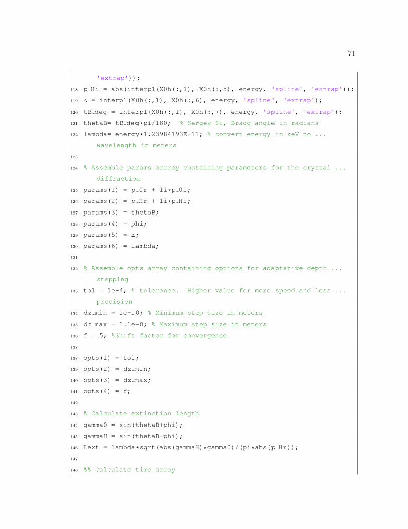
71
'extrap'));
118 p Hi = abs(interp1(X0h(:,1), X0h(:,5), energy, 'spline', 'extrap'));
119 ∆ = interp1(X0h(:,1), X0h(:,6), energy, 'spline', 'extrap');
120 tB deg = interp1(X0h(:,1), X0h(:,7), energy, 'spline', 'extrap');
121 thetaB= tB deg*pi/180; % Sergey Si, Bragg angle in radians
122 lambda= energy*1.23984193E-11; % convert energy in keV to ...
wavelength in meters
123
124 % Assemble params arrray containing parameters for the crystal ...
diffraction
125 params(1) = p 0r + 1i*p 0i;
126 params(2) = p Hr + 1i*p Hi;
127 params(3) = thetaB;
128 params(4) = phi;
129 params(5) = ∆;
130 params(6) = lambda;
131
132 % Assemble opts array containing options for adaptative depth ...
stepping
133 tol = 1e-4; % tolerance. Higher value for more speed and less ...
precision
134 dz min = 1e-10; % Minimum step size in meters
135 dz max = 1.1e-8; % Maximum step size in meters
136 f = 5; %Shift factor for convergence
137
138 opts(1) = tol;
139 opts(2) = dz min;
140 opts(3) = dz max;
141 opts(4) = f;
142
143 % Calculate extinction length
144 gamma0 = sin(thetaB+phi);
145 gammaH = sin(thetaB-phi);
146 Lext = lambda*sqrt(abs(gammaH)*gamma0)/(pi*abs(p Hr));
147
148 %% Calculate time array
72
149 if time == 0
150 time = time f; % set default maximum time delay to default
151 end
152 if (length(time)==1)
153 dt =time; % save for external file function
154 time = time/num times:time/num times:time;
155 end
156
157 %% Calculate angular array
158 if (angle == 0)
159 angle = angle width; % set default angular width to 10 mdeg
160 end
161 if (length(angle)==1)
162 angle = (0:angle/num angles:angle)-0.9*angle/2;
163 end
164
165 angle = thetaB + angle*pi/180; % Convert angle to radians and ...
add Bragg Angle
166
167 if strcmp(model,'thermalFilm')
168 [longitudinal trans sheer time out z] = thermalFilm (film, ...
crystal, fluence, time, 5.1*Lext, L);
169 elseif strcmp(model,'strainFile')
170 z = load('depth file.txt');
171 time out = load('time file.txt');
172 longitudinal = load('strain file.txt');
173 trans = 0*longitudinal;
174 sheer = 0*longitudinal;
175 elseif strcmp(model,'strainFile1D') % strains just at one time
176 z = load('depth file.txt');
177 time file = load('time file.txt');
178 time out = time file(fluence); % No time specified, just ...
strain at one time
179 all strain = load('strain file.txt');
180 longitudinal = all strain(floor(fluence),:); % load only one ...
column
73
181 trans = 0*longitudinal;
182 sheer = 0*longitudinal;
183 time=time out;
184 elseif strcmp(model,'benchmark')
185 clear time;
186 time = 1;
187 time out = 1;
188 dz = 5.1*Lext/10000; % 10,000 depth points out to 5.1*Lext
189 z = dz*(1:10000);
190 trans = 0.*z; % no transverse strain
191 sheer = 0.*z; % no sheer strain
192 %longitudinal = 0.*z;
193 longitudinal = 1e-4 * (z≤2e-6); % Simple strain model
194 else
195 fprintf('Not a valid model\n')196 return
197 end
198
199 % Need to add a single timepoint test for comparisson with ...
Sergey's GID
200 % Otherwise seems to work 12/28/16 EL
201
202 for m = 1: length(time)
203 fprintf('Evaluating rocking curve at %e s.\n',time out(m))
204 if time(m) == time out(m) % if the time doesn't need to be ...
remeshed
205 st1(m,:) = longitudinal(m,:);
206 st2(m,:) = trans(m,:);
207 st3(m,:) = sheer(m,:);
208 else % remesh time if necessary
209 st1(m,:) = interp1(time out,longitudinal,time(m), 'spline', ...
'extrap');
210 st2(m,:) = interp1(time out,trans,time(m), 'spline', 'extrap');
211 st3(m,:) = interp1(time out,sheer,time(m), 'spline', 'extrap');
212 end
213 Strain in = [st1(m,:)' st2(m,:)' st3(m,:)']; % Evaluate strain ...
74
at each time
214 [X X0 err Steps Strain out] = WieAdapt (Strain in, z, angle, ...
opts, params);
215 A0 = X0.*conj(X0); % Unstrained crystal intensity
216 A(m,:) = X.*conj(X); % Intensity Amplitude
217 Strain save(m,:,:) = Strain out(:,:);
218 % x = 1:10000;
219 % strainsave = sprintf('strain%d.png',m);
220 %
221 % figure
222 % plot(x, Strain out(:,:))
223 % saveas(gcf,strainsave)
224 end
225
226 if strcmp(model,'benchmark')
227 % Keep angle in absolute radians
228 angle = (angle)*180/pi; % Convert angle back to degrees ...
relative to Bragg
229 else
230 angle = (angle)*180/pi; % Convert angle back to degrees ...
relative to Bragg
231 end
232
233 figure
234 plot(angle,A)
235 xlabel('Angle')
236 ylabel('Intensity')
237
238 % rang1 = (-60:0.3:60);
239 % rang2 = (-60:0.2308:60.2308);
240 % rang3 = (-60:1:60);
241 %
242 % phi = rang1 * (pi/360);
243 %
244 % res = exp( -(phi.ˆ2)/(den));
245 %
75
246 % convol = conv(A,res);
247 %
248 % plot(rang3,rocking/max(rocking))
249 % hold on
250 % plot(rang2,convol)
251 % xlabel('Angle')
252 % ylabel('Normalized Intensity')
253 % legend('Experimental','Theoretical')
254
255
256 % T = [angle; A0];
257 %
258 % fileID = fopen('tabledata.txt','w');
259 % fprintf(fileID,'%6s %12s\n','angle','intensity');260 % fprintf(fileID,'%6.2f %12.8f\n',T);261 % fclose(fileID);
262
263 %hold on
264
265 %plot(Output.Angle,Output.Intensity)
1 %This script will run a loop comparing the theoretical and ...
experimental
2 %rocking curves obtained from TRXD.
3 %
4 %
5 %
6 %
7 %Variables
8 % n The number of iterations we want to run the script for
9 % RoCur The experimental rocking curve data we are ...
interested in
10 % control The TRXD results for the data we are interested in
11 % Ang The angles for our experimental rocking curve data
12 % std The denominator for the exponential in the gaussian
76
13 % Time The time table for our experimental rocking curve data
14 % a The asymmetry factor for the asymmetrical lorentzian
15
16 function TRXDloop(n,RoCur,Ang,std,a,model, film, crystal, ...
reflection, cut, energy, fluence, angle, time, L, ...
gaussianwidth, lorentzianwidth, offset)
17 %run TRXD
18 [A A0 time angle Strain save z] = TRXD (model, film, ...
crystal, reflection, cut, energy, fluence, angle, time, L);
19
20 %surfacedata = [];
21
22 %this for loop allows the comparison function to be run as ...
many times
23 %as needed without having to manually change inputs multiple ...
times
24
25
26 for c = 1:n
27 %create the save names for the plots
28 svnmlin = sprintf('lintimestamp%d.png',c);
29 svnmlog = sprintf('logtimestamp%d.png',c);
30
31 %the comparison function
32 [convol] = ...
comparison(RoCur(:,c),A(c,:),std,svnmlin,svnmlog,Ang(1,c),Ang(121,c),Ang(:,c),time(1,c),a);
33
34 %surfacedata(n,:) = convol;
35
36 end
37
38 %figure
39 %surf(surfacedata,'edgecolor','none')
40
41 end
42
77
43
44 function [convol] = ...
comparison(rocur,control,den,linname,logname,rangb,range,ang,time,a)
45
46 %convert sample data tables to arrays
47 beginning = table2array(rangb);
48 finish = table2array(range);
49 rocking = table2array(rocur);
50 angles = table2array(ang);
51
52
53
54 %create ranges based off of angles for the sample. rang is for ...
plotting
55 %the resolution function, rangconvol is for plotting the convolution
56 rang = (beginning:0.3:finish);
57 rangconvol = (beginning:0.15:finish);
58
59 %convert range of angles to radians
60 phi = rang * (pi/180);
61
62 %laser resolution function
63 %res = exp( -(phi.ˆ2)/(den));
64 % gamma = (2*60)./(1 + exp(a*phi));
65 % res = (2./(pi*gamma))./(1 + 4*(phi./gamma).ˆ2);
66
67
68
69 %convolve theoretical rocking curve with function used to test laser
70 %resolution
71 convol = conv(control,res);
72
73
74
75 %for troubleshooting - most common error so far seems to be ...
lengths not
78
76 %matching
77
78 % convol/max(convol)
79 % res/max(res)
80 % control/max(control)
81
82 % length(rangconvol)
83 % length(convol)
84 % length(res)
85
86 % length(rocking)
87 % length(angles)
88
89 %create and save linear figure comparing theoretical and ...
experimental
90 %rocking curves
91
92 % figure
93 % plot(rang,res)
94
95 figure
96 plot(angles,rocking/max(rocking))
97 hold on
98 plot((rangconvol-5.55),convol/max(convol))
99 %xlim([-5 5])
100 xlabel('Angle')
101 ylabel('Normalized Intensity')
102 legend('Experimental','Theoretical')
103 title(['Timestamp ', num2str(time), ' seconds'])
104 saveas(gcf,linname)
105
106 %create and save logarithmic figure comparing theoretical and ...
experimental
107 %rocking curves
108 figure
109 semilogy(angles,rocking/max(rocking))
79
110 hold on
111 semilogy((rangconvol-5.55),convol/max(convol))
112 %xlim([-5 5])
113 ylim([1e-3 1])
114 xlabel('Angle')
115 ylabel('Normalized Intensity')
116 legend('Experimental','Theoretical')
117 title(['Timestamp ', num2str(time), ' seconds'])
118 saveas(gcf,logname)
119
120 end
1 function [temperature strain] = shift2temp(thetaShift, ...
thetaBragg, crystal);
2 % determine average temperature shift from average Bragg peak shift
3 % Eric Landahl, June 25, 2021
4 % INPUTS
5 % thetaShift Bragg angle shift IN DEGREES
6 % thetaBragg Bragg angle OM DEGREES
7 % crystal String of crystal abbreviation, e.g. 'Si'
8 % OUTPUT
9 % temperature Average temperature change in deg K
10 % strain unitless, ∆-d / d (d is lattice spacing)
11 % REQUIRES
12 % sampledata
13 % EXAMPLE USAGE
14 % [temperature strain] = shift2temp(-1e-3,27.24,'GaAs')
15 % should return 5.9 deg K temperature increase, stain of ...
3.4e-5
16 % OTHER USAGE
17 % Calculate strain/temperature to check thermal expasion ...
coef. alpha t
18 % ex: strain/temperature = 5.73e-6 1/K for example above
19
20 % Convert to radians
80
21 thetaShift = thetaShift*pi/180;
22 thetaBragg = thetaBragg*pi/180;
23
24 sampledata % load material properties
25 ID = find(strcmp({sample.name}, crystal)==1);
26 alpha t = sample(ID).thermalExpansion.val; % 1/K
27
28 strain = - thetaShift * cot(thetaBragg);
29 temperature = strain/alpha t;
1 %JimmyFigs.m
2 % Making extra figures for J. Grammich MS Thesis
3 % E. Landahl, 6-25-21
4 %
5 % REQUIRES
6 % dataLoader.m must have already been run to save workspace ...
of data and
7 % simulations
8 % shift2temp.m needed to calculate temperature shifts from ...
angle shifts
9 %
10 clear all;
11 close all;
12 load('GaAs 100nm data.mat'); % Load entire workspace
13
14 %% . OLD STUFF, IGNORE
15 % blur = 72;
16 % A = smoothdata(AA,2,'gaussian',blur); % Convolve with ...
experimental angular resolution
17 % A0 = smoothdata(AA0,'gaussian',blur);
18
19 %theta0 = theta0 - 0.0005; % Account for shift between theory ...
and data
20
21 clear A
81
22 clear A0
23
24 f = AA0; % unstrained simulation result
25 gamma = 0.00035; % Cauchy width of instrument in degrees
26 sigma = 0.00145; % Gaussian width of instrument in degrees
27 g1 = (1/(sigma*sqrt(2*pi)))*exp(-0.5*(dtheta./sigma).ˆ2); % Gaussian
28 g2 = (gamma/pi)./(dtheta.ˆ2 + gammaˆ2); % Cauchy / Lorentzian
29 g = conv(g1,g2,'same'); % Voigt
30 g = g/max(g);
31 h = conv(f,g,'same'); % to compare to measurement
32 h = h + .005; % add offset
33 h = h/max(h);
34 g1 = (1/(sigma*sqrt(2*pi)))*exp(-0.5*(dtheta./sigma).ˆ2); % Gaussian
35 g2 = (gamma/pi)./(dtheta.ˆ2 + gammaˆ2); % Cauchy / Lorentzian
36 g = conv(g1,g2,'same'); % Voigt
37 g = g/max(g);
38 h = conv(f,g,'same'); % to compare to measurement
39 h = h + .005; % add offset
40 h = h/max(h);
41
42 A0 = h;
43
44 for j = 1: length(newTime)
45 f = AA(j,:);
46 g1 = (1/(sigma*sqrt(2*pi)))*exp(-0.5*(dtheta./sigma).ˆ2); % ...
Gaussian
47 g2 = (gamma/pi)./(dtheta.ˆ2 + gammaˆ2); % Cauchy / Lorentzian
48 g = conv(g1,g2,'same'); % Voigt
49 g = g/max(g);
50 h = conv(f,g,'same'); % to compare to measurement
51 h = h + .005; % add offset
52 h = h/max(h);
53 A(j,:) = h;
54 end
55
56 %theta0 = theta0-.0005;
82
57
58 %% Centroid shifts from calculations
59 center0 = centroid(dtheta,A0); %A0 is calculated unstrained ...
rocking curve
60 for i = 1:length(newTime)
61 centerShiftCalc(i) = 1000*(centroid(dtheta,A(i,:))-center0);
62 end
63
64 %% This figure just shows the calculation results
65 figure(3);clf;hold on
66 plot(newTime,centerShiftCalc,'-')
67 xlabel('Time (ns)')
68 ylabel('Cetroid Shift Calculated (mdeg)')
69 %title('GaAs with 100 nm Cr coating')
70 legend(gca,'off')
71 ax = gca;
72 ax.FontSize = 16;
73 hold off;
74
75 %% Add calcs to linear centroid shift plot
76 % figure(1);hold on
77 % plot(newTime,centerShiftCalc,'.r','LineWidth',2)
78 % saveas(1,['¬/Documents/Jimmy/figures/LinSim+Data.png'])79 % saveas(1,['¬/Documents/Jimmy/figures/LinSim+Data.fig'])80 % saveas(1,['¬/Documents/Jimmy/figures/LinSim+Data.eps'])81 % hold off
82 %
83 % %% Add calcs to log centroid shift plot
84 % figure(2);hold on
85 % semilogx(newTime,centerShiftCalc,'.r','LineWidth',2)
86 % saveas(2,['¬/Documents/Jimmy/figures/LogSim+Data.png'])87 % saveas(2,['¬/Documents/Jimmy/figures/LogSim+Data.fig'])88 % saveas(2,['¬/Documents/Jimmy/figures/LogSim+Data.eps'])89 % hold off
90
91 %% Simulation surface plots
83
92 figure(6);clf; hold on;
93 surf(dtheta+theta0,newTime,A);
94 shading interp;
95 ylim([0 max(timePos)]);
96 xlim([27.239 27.255])
97 xlabel('Theta (degrees)')
98 ylabel('Time (ns)')
99 title('100 nm Cr film on GaAs Simulation')
100 ax = gca; ax.FontSize=16;
101 saveas(6,['¬/Documents/Jimmy/figures/LinSim.png'])102 saveas(6,['¬/Documents/Jimmy/figures/LinSim.fig'])103 saveas(6,['¬/Documents/Jimmy/figures/LinSim.eps'])104 hold off
105
106 figure(7);clf; hold on;
107 surf(dtheta+theta0,newTime,log(A));
108 ylim([0.048 5]); shading interp;
109 xlabel('Theta (degrees)')
110 ylabel('Time (ns)')
111 title('100 nm GaAs Simulation (Log Scale)')
112 ax = gca; ax.FontSize=16;
113 saveas(7,['¬/Documents/Jimmy/figures/LogSim.png'])114 saveas(7,['¬/Documents/Jimmy/figures/LogSim.fig'])115 saveas(7,['¬/Documents/Jimmy/figures/LogSim.eps'])116 hold off
117
118 %% Plots at particular timepoints
119 % Hint: k = find(abs(timePos-5) < 0.05 to find index k near 5 ns
120
121 k0 = 1; % Before time zero
122 timek0 = newTime(k0);
123 % figure(8);clf;hold on
124 % plot(theta,On(k0,:)/max(On(k0,:)),'bo')
125 % plot(dtheta+theta0,A0/max(A0),':b')
126 % text(27.24,.9,[num2str(timek0,'%.1f') ' ns'],'FontSize',16)
127 % xlabel('\theta (degrees)')
84
128 % ylabel('Normalized Intensity')
129 % xlim([27.239 27.255])
130 % ax = gca; ax.FontSize=16;
131 % saveas(8,['¬/Documents/Jimmy/figures/Unstrained LinRock.png'])
132 % saveas(8,['¬/Documents/Jimmy/figures/Unstrained LinRock.eps'])
133 % saveas(8,['¬/Documents/Jimmy/figures/Unstrained LinRock.fig'])
134 % hold off;
135 % figure(9);clf;
136 % semilogy(theta,On(k0,:)/max(On(k0,:)),'bo');hold on;
137 % semilogy(dtheta+theta0,A0/max(A0),':b')
138 % text(27.19,.5,[num2str(timek0,'%.1f') ' ns'],'FontSize',16)
139 % xlabel('\theta (degrees)')
140 % ylabel('Normalized Intensity')
141 % ax = gca; ax.FontSize=16;
142 % saveas(9,['¬/Documents/Jimmy/figures/Unstrained LogRock.png'])
143 % saveas(9,['¬/Documents/Jimmy/figures/Unstrained LogRock.eps'])
144 % saveas(9,['¬/Documents/Jimmy/figures/Unstrained LogRock.fig'])
145 % hold off;
146
147 k05 = 10; % 0.5 ns;
148 k1 = 21; % 1 ns
149 k5 = 64; % 5 ns
150 k10 = 71; % 10 ns
151 k25 = 92; %25 ns
152 k50 = 104; % 50 ns
153 k100 = 124; % 100 ns
154 k250 = 163; % 250 ns
155 k500 = 209; % 500 ns
156 k750 = 258; % 750 ns
157 k1000 = 305; % 1 us
158 k1250 = 351; % 1.25 us
159 k1500 = 399; % 1.5 us
160 k1750 = 446; %1.75 us
161 k2000 = 493; % 2 us
162 k2250 = 541; % 2.25 us
163 k2500 = 588; % 2.5 us
85
164 k2750 = 636; % 2.75 us
165 k3000 = 683; % 3 us
166 k3250 = 729; % 3.25 us
167
168
169 k = [k0 k05 k1 k5 k10 k25 k50 k100 k250 k500 k750 k1000 k1250 ...
k1500 k1750 k2000 k2250 k2500 k2750 k3000 k3250];
170 timek = newTime(k);
171 is = 118; % index shifter for data vs simulation
172 thetaBmp = -0.001;
173 for i = 1:length(k)
174 figure(7+i);clf;hold on;
175 plot(theta+theta0-thetaBmp-centerOff(k(i)+is),On(k(i)+is,:)/max(On(k(i)+is,:)),'ro','MarkerFaceColor','r')
176 plot(theta+theta0-thetaBmp-centerOff(k(i)+is),Off(k(i)+is,:)/max(Off(k(i)+is,:)),'bo')
177 plot(dtheta+theta0,A(k(i),:)/max(A(k(i),:)),'-r','LineWidth',2)
178 plot(dtheta+theta0,A0/max(A0),':b','LineWidth',2)
179 text(27.24,.9,[num2str(newTime(k(i)),'%.1f') ' ...
ns'],'FontSize',16)
180 xlabel('\theta (degrees)')
181 ylabel('Normalized Intensity')
182 xlim([27.239 27.255]);
183 ax = gca; ax.FontSize=16;
184 saveas(7+i,['¬/Documents/Jimmy/figures/' ...
num2str(timek(i),'%.1f') 'ns ''LinRock.png'])
185 saveas(7+i,['¬/Documents/Jimmy/figures/' ...
num2str(timek(i),'%.1f') 'ns ''LinRock.eps'])
186 saveas(7+i,['¬/Documents/Jimmy/figures/' ...
num2str(timek(i),'%.1f') 'ns ''LinRock.fig'])
187 end
188
189
190
191 for i = 1:length(k)
192 figure(29+i);clf;
193 semilogy(theta+theta0-thetaBmp-centerOff(k(i)+is),On(k(i)+is,:)/max(On(k(i)+is,:)),'ro','MarkerFaceColor','r');hold ...
on;
86
194 semilogy(theta+theta0-thetaBmp-centerOff(k(i)+is),Off(k(i)+is,:)/max(Off(k(i)+is,:)),'bo');
195 semilogy(dtheta+theta0,A(k(i),:)/max(A(k(i),:)),'-r','LineWidth',2)
196 semilogy(dtheta+theta0,A0/max(A0),':b','LineWidth',2)
197 text(27.205,.5,[num2str(newTime(k(i)),'%.1f') ' ...
ns'],'FontSize',16)
198 xlabel('\theta (degrees)')
199 ylabel('Normalized Intensity')
200 xlim([27.2 27.3]);
201 ylim([1e-4 2]);
202 ax = gca; ax.FontSize=16;
203 saveas(29+i,['¬/Documents/Jimmy/figures/' ...
num2str(timek(i),'%.1f') 'ns ''LogRock.png'])
204 saveas(29+i,['¬/Documents/Jimmy/figures/' ...
num2str(timek(i),'%.1f') 'ns ''LogRock.eps'])
205 saveas(29+i,['¬/Documents/Jimmy/figures/' ...
num2str(timek(i),'%.1f') 'ns ''LogRock.fig'])
206 end
207
208
209 %% Surface plots
210 figure(4);clf; hold on;
211 surf(theta,timePos,OnPos);
212 shading interp;
213 ylim([0 max(timePos)])
214 xlim([27.239 27.255])
215 xlabel('Theta (degrees)')
216 ylabel('Time (ns)')
217 title('100 nm Cr film on GaAs Data')
218 ax = gca; ax.FontSize=16;
219 hold off
220
221 figure(5);clf; hold on;
222 surf(theta,timePos,log(OnPos)); caxis([-11 -2.7]);
223 zlim([-11 -2.7]); ylim([0.048 5]); shading interp;
224 xlabel('Theta (degrees)')
225 ylabel('Time (ns)')
87
226 title('100 nm GaAs Data (Log Scale)')
227 ax = gca; ax.FontSize=16;
228 hold off
229
230
231 temperature = shift2temp(centerShift/1000, theta0, 'GaAs');
232
233 %% Linear Plot
234 figure(1); clf; hold on;
235 yyaxis left
236 h1 = plot(time,centerShift,'ro')
237 h2 = plot(newTime,centerShiftCalc,'-k','LineWidth',2)
238 xlabel('Time (ns)')
239 ylabel('Centroid shift (mdeg)')
240 yyaxis right
241 h3 =plot(time,temperature,'Marker','none','LineStyle','none')
242 ax = gca;
243 ax.YDir = 'reverse'
244 ylabel('Temperature shift (K)')
245 ax.YAxis(1).Color = 'k';
246 ax.YAxis(2).Color = 'k';
247 ax.FontSize = 16;
248
249 % Inset
250 bx = axes('Position',[.5 .2 .3 .3])
251 hold on;
252 plot(time,centerShift,'ro')
253 plot(newTime,centerShiftCalc,'-k','LineWidth',2)
254 xlim([-10 50]);
255 bx.FontSize = 16;
256 bx.TickLength = [0.02 0.02];
257 bx.LineWidth = 1;
258
259 hold off
260
261 %% Log Plot
88
262 figure(2); clf;
263 yyaxis left
264 h1 = semilogx(time,centerShift,'ro');
265 hold on;
266 h2 = semilogx(newTime,centerShiftCalc,'-k','LineWidth',2)
267 xlabel('Time (ns)')
268 ylabel('Centroid shift (mdeg)')
269 yyaxis right
270 h3 = ...
semilogx(time,temperature,'Marker','none','LineStyle','none')
271 ax = gca;
272 ax.YDir = 'reverse'
273 ylabel('Temperature shift (K)')
274 ax.YAxis(1).Color = 'k';
275 ax.YAxis(2).Color = 'k';
276 ax.FontSize = 16;
277 hold off
278
279
280 %% Plots for trouble shooting (not saved)
281 %
282 % is = 119; % index shifter for data vs simulation
283 %
284 % for i = 1:length(newTime)
285 % k(i)=i;
286 % figure(200);clf;hold on;
287 % ...
plot(theta+theta0-thetaBmp-centerOff(k(i)+is),On(k(i)+is,:)/max(On(k(i)+is,:)),'ro','MarkerFaceColor','r')
288 % ...
plot(theta+theta0-thetaBmp-centerOff(k(i)+is),Off(k(i)+is,:)/max(Off(k(i)+is,:)),'bo')
289 % plot(dtheta+theta0,A(k(i),:)/max(A(k(i),:)),'-r')
290 % plot(dtheta+theta0,A0/max(A0),':b')
291 % text(27.24,.9,[num2str(newTime(k(i)),'%.1f') ' ...
ns'],'FontSize',16)
292 % xlabel('\theta (degrees)')
293 % ylabel('Normalized Intensity')
89
294 % xlim([27.239 27.255])
295 % ax = gca; ax.FontSize=16;
296 % title(num2str(centerShift(i)));
297 % hold off;
298 %
299 % figure(201);clf;
300 % ...
semilogy(theta+theta0-thetaBmp-centerOff(k(i)+is),On(k(i)+is,:)/max(On(k(i)+is,:)),'ro','MarkerFaceColor','r');hold ...
on;
301 % ...
semilogy(theta+theta0-thetaBmp-centerOff(k(i)+is),Off(k(i)+is,:)/max(Off(k(i)+is,:)),'bo');
302 % semilogy(dtheta+theta0,A(k(i),:)/max(A(k(i),:)),'-r')
303 % semilogy(dtheta+theta0,A0/max(A0),':b')
304 % text(27.19,.5,[num2str(newTime(k(i)),'%.1f') ' ...
ns'],'FontSize',16)
305 % xlabel('\theta (degrees)')
306 % ylabel('Normalized Intensity')
307 % ax = gca; ax.FontSize=16;
308 % title(num2str(centerShift(i)));
309 % hold off;
310 % i
311 % jnk = input('Press Enter to Continue')
312 % end
313 %
90
REFERENCES
[1] Jean Baptiste Joseph Baron Fourier. The analytical theory of heat. The Uni-
versity Press, 1878.
[2] Timothy S Fisher. Thermal energy at the nanoscale, volume 3. World Scientific
Publishing Company, 2013.
[3] David G Cahill, Paul V Braun, Gang Chen, David R Clarke, Shanhui Fan,
Kenneth E Goodson, Pawel Keblinski, William P King, Gerald D Mahan, Arun
Majumdar, et al. Nanoscale thermal transport. ii. 2003–2012. Applied physics
reviews, 1(1):011305, 2014.
[4] Keith T Regner, Justin P Freedman, and Jonathan A Malen. Advances in
studying phonon mean free path dependent contributions to thermal conduc-
tivity. Nanoscale and Microscale Thermophysical Engineering, 19(3):183–205,
2015.
[5] Li Shi, Chris Dames, Jennifer R Lukes, Pramod Reddy, John Duda, David G
Cahill, Jaeho Lee, Amy Marconnet, Kenneth E Goodson, Je-Hyeong Bahk,
et al. Evaluating broader impacts of nanoscale thermal transport research.
Nanoscale and Microscale Thermophysical Engineering, 19(2):127–165, 2015.
[6] RB Wilson, Brent A Apgar, Lane W Martin, and David G Cahill. Ther-
moreflectance of metal transducers for optical pump-probe studies of thermal
properties. Optics express, 20(27):28829–28838, 2012.
[7] Austin J Minnich, Jeremiah A Johnson, Aaron Jerome Schmidt, Keivan Esfar-
jani, Mildred Spiewak Dresselhaus, Keith A Nelson, and Gang Chen. Thermal
conductivity spectroscopy technique to measure phonon mean free paths. Phys-
ical review letters, 107(9):095901, 2011.
91
[8] Keith T Regner, Daniel P Sellan, Zonghui Su, Cristina H Amon, Alan JH
McGaughey, and Jonathan A Malen. Broadband phonon mean free path con-
tributions to thermal conductivity measured using frequency domain thermore-
flectance. Nature communications, 4(1):1–7, 2013.
[9] Ashok T Ramu and Yanbao Ma. An enhanced fourier law derivable from the
boltzmann transport equation and a sample application in determining the
mean-free path of nondiffusive phonon modes. Journal of Applied Physics,
116(9):093501, 2014.
[10] CW Li, Olle Hellman, Jie Ma, AF May, HB Cao, X Chen, AD Christianson,
G Ehlers, DJ Singh, BC Sales, et al. Phonon self-energy and origin of anomalous
neutron scattering spectra in snte and pbte thermoelectrics. Physical review
letters, 112(17):175501, 2014.
[11] M Highland, BC Gundrum, Yee Kan Koh, Robert S Averback, David G Cahill,
VC Elarde, JJ Coleman, DA Walko, and EC Landahl. Ballistic-phonon heat
conduction at the nanoscale as revealed by time-resolved x-ray diffraction and
time-domain thermoreflectance. Physical Review B, 76(7):075337, 2007.
[12] Yu-Miin Sheu, M Trigo, YJ Chien, C Uher, DA Arms, ER Peterson, DA Walko,
EC Landahl, J Chen, S Ghimire, et al. Kapitza conductance of bi/sapphire
interface studied by depth-and time-resolved x-ray diffraction. Solid state com-
munications, 151(11):826–829, 2011.
[13] G Jackson Williams, Sooheyong Lee, Donald A Walko, Michael A Watson,
Wonhuyk Jo, Dong Ryeol Lee, and Eric C Landahl. Direct measurements of
multi-photon induced nonlinear lattice dynamics in semiconductors via time-
resolved x-ray scattering. Scientific reports, 6(1):1–10, 2016.
[14] G Jackson Williams, Michael A Watson, Dohn A Arms, Timothy M Mooney,
Donald A Walko, and Eric C Landahl. Epics oscilloscope for time-resolved data
acquisition. Nuclear Instruments and Methods in Physics Research Section A:
92
Accelerators, Spectrometers, Detectors and Associated Equipment, 649(1):84–
86, 2011.
[15] CR Wie, TA t Tombrello, and T Vreeland Jr. Dynamical x-ray diffraction
from nonuniform crystalline films: Application to x-ray rocking curve analysis.
Journal of applied physics, 59(11):3743–3746, 1986.
[16] Sergei G Podorov, G Holzer, E Forster, and NN Faleev. Semidynamical solu-
tion of the inverse problem of x-ray bragg diffraction on multilayered crystals.
physica status solidi (a), 169(1):9–16, 1998.
[17] AA Stepanov. Fourier-coefficient method of x-ray rocking-curve interpretation.
Journal of applied crystallography, 27(1):7–12, 1994.
[18] Sooheyong Lee, G Jackson Williams, Maria I Campana, Donald A Walko, and
Eric C Landahl. Picosecond x-ray strain rosette reveals direct laser excitation
of coherent transverse acoustic phonons. Scientific reports, 6(1):1–7, 2016.
[19] David W Hahn and M Necati Ozisik. Heat conduction. John Wiley & Sons,
2012.
[20] Zlatan Aksamija. Nanophononics: Thermal Generation, Transport, and Con-
version at the Nanoscale. CRC Press, 2017.
[21] Bertram Eugene Warren. X-ray Diffraction. Courier Corporation, 1990.
[22] Sergey A Stepanov. X-ray server: an online resource for simulations of x-ray
diffraction and scattering. In Advances in Computational Methods for X-Ray
and Neutron Optics, volume 5536, pages 16–26. International Society for Optics
and Photonics, 2004.
[23] Sergey A Stepanov. X-ray server, 2004. Available at https://x-
server.gmca.aps.anl.gov.
[24] Eric C Landahl. Time-resolved x-ray diffraction, 2008. Available at
https://github.com/elandahl/dynamical-diffraction.
93
[25] John D’Errico. Slm - shape language modeling, 2017. Available
at https://www.mathworks.com/matlabcentral/fileexchange/24443-slm-shape-
language-modeling.