Embed Size (px)
Citation preview
Electromagnetic Response for High-Frequency Gravitational Waves in the GHz to THz Band∗
Fang-Yu Li†, Meng-Xi Tang††, and Dong-Ping Shi†††
† Department of Physics, Chongqing University, Chongqing 400044, China,
E-mail: [email protected]
†† Department of Physics, Zhongshan University, Guangzhou 510275, China,
E-mail: [email protected]
††† Department of Physics, Chongqing University, Chongqing 400044, China,
E-mail: [email protected]
ABSTRACT
We consider the electromagnetic (EM) response of a Gaussian beam passing through a static
magnetic field to be the high-frequency gravitational waves (HFGW) as generated by several devices
discussed at this conference. It is found that under the synchroresonance condition, the first-order
perturbative EM power fluxes will contain a “left circular wave” and a “right circular wave” around the
symmetrical axis of the Gaussian beam. However, the perturbative effects produced by the states of +
polarization and × polarization of the GW have a different physical behavior. For the HFGW of
(which corresponds to the power flux density ) to ,
(which corresponds to the power flux density ) expected by the HFGW
generators described at this conference, the corresponding perturbative photon fluxes passing through a
surface region of 10 would be expected to be 10 . They are the orders of
magnitude of the perturbative photon flux we estimated using typical laboratory parameters that could
lead to the development of sensitive HFGW receivers. Moreover, we will also discuss the relative
background noise problems and the possibility of displaying the HFGW. A laboratory test bed for
juxtaposed HFGW generators and our detecting scheme is explored and discussed.
300−=3 , 1g GHz hν =
2810h −=
6 2~ 10 W m− −⋅
3 2W m−⋅
4 110 s− −
1.3g THzν =
~ 10
3 1s −2 2m−
∗ Invited talk at the first international conference on High-Frequency Gravitational Waves, Paper-03-108, May 2003, The MITRE Corporation, McLean, Virginia, USA.
1
I INTRODUCTION
In recent years, since suggestion of a serried of new theoretical models and physical ideas [1, 2,
3], and fast development of relative technology (such as nanotechnology, ultra-fast science,
high-temperature superconductors, ultra-strong laser physics, high energy laboratory astrophysics, etc.,
[4-9]), these results offered new possibilities for laboratory generation and detection of high-frequency
gravitational waves (HFGW).
In this paper we shall study the electromagnetic (EM) response to the HFGW in the GHz-THz
band. Our EM detecting system is a Gaussian beam passing through a static magnetic field. Here we
consider it since there are following reasons: (1) Unlike the EM response to the gravitational waves
(GW’s) by an ideal plane EM wave, the Gaussian beam is a realized EM wave beam satisfying physical
boundary conditions, and because of the special property of the Gaussian function of the beam, whether
the GHz band or the THz region, the EM response has good space accumulation effect. (2) In recent
years, strong and ultra-strong lasers and microwave beams have been generated [6-8] under the
laboratory conditions, and many of the beams are often expressed as the Gaussian-type or the
quasi-Gaussian-type, and they usually have good monochromaticity in the GHz to THz band. (3) The
EM response in the GHz to THz band means that the dimensions of the EM detecting system may be
reduced to the typical laboratory size (e.g., magnitude of meter). (4) The GHz and THz band are just
typical frequency regions expected by the HFGW generators described at this conference (see relevant
references in this conference). (5) The Gaussian beam propagating through a static magnetic field is an
open system; in this case the EM perturbation might have more direct displaying effect. Therefore, the
EM response of the Gaussian beam and other means discussed at this conference have a good
complementarity.
II THE ELECTROMAGNETIC DETECTING SYSTEM: A GAUSSIAN BEAM PASSING
THROUGH A STATIC MAGNETIC FIELD.
It is well known that in flat spacetime (i.e., when the GW’s are absent) usual form of the
fundamental Gaussian beam is given by [10]
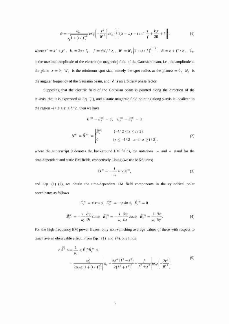
( )
210
22exp exp tan ,
21 /e
e ek rr zi k z t
W fz f
ψψ ω −
Rδ = − − − + + +
(1)
where , , , 2 2r x y= + 2 2 /e ek π λ= 20 / ef Wπ λ= ( )
1/220 1 /W W z f = + , ,
is the maximal amplitude of the electric (or magnetic) field of the Gaussian beam, i.e., the amplitude at
the plane , is the minimum spot size, namely the spot radius at the plane z , is
the angular frequency of the Gaussian beam, and is an arbitrary phase factor.
2 /R z f z= +
0=
0ψ
e0z = W0 ω
δ
Supposing that the electric field of the Gaussian beam is pointed along the direction of the
-axis, that it is expressed as Eq. (1), and a static magnetic field pointing along y-axis is localized in
the region− ≤ , then we have
x
/2 /2l z l≤
( ) ( ) ( ) ( )0 0 0 0, 0x y zE E E Eψ= = = = ,
/2 , (2) ( ) ( )0 0ˆ ,B B=
( ) ( )
( )0ˆ /2 /2
0 /2 and
yB l z l
z l z l
− ≤ ≤= ≤− ≥
where the superscript 0 denotes the background EM fields, the notations and ^ stand for the
time-dependent and static EM fields, respectively. Using (we use MKS units)
∼
( ) ( )0 ,e
iω
= − ∇×B 0E
0
(3)
and Eqs. (1) (2), we obtain the time-dependent EM field components in the cylindrical polar
coordinates as follows
( ) ( ) ( )0 0cos , sin , 0,r zE E Eφψ φ ψ φ= = − =
( ) ( ) ( )0 0 0sin , cos , .r ze e
i iB B B
z zφψ ψφ φ
ω ω∂ ∂= − = − =∂ ∂ e
iyψ
ω∂∂
(4)
For the high-frequency EM power fluxes, only non-vanishing average values of these with respect to
time have an observable effect. From Eqs. (1) and (4), one finds
( )( ) ( )
( )( )( )
00 0
0
2 2 22 20
2 2 2 22 2 20
1
2exp ,2 1 / 2
zx y
ee
e
S E B
k r f z f rkf z Wz f f z
µ
ψµ ω
< >= < >
− = + − − + + +
(5)
3
( )( ) ( )
( ) ( )
00 0
0
2 2 20
22 20
1
sin 2exp ,2 1 / /
rz
e
e
S E B
k r rWz f z f z
φµψ φ
µ ω
< >= < >
= − + +
(6)
( )( ) ( )
( )( ) ( )
00 0
02 20
22 20
1
sin 2 2exp ,4 1 / /
r z
e
e
S E B
k r rWz f z f z
φ
µψ φ
µ ω
< >= − < >
= − + +
(7)
where represent the average values of the axial, radial and tangential
EM power flux densities, respectively, the angular brackets denote the average values with respect to
time. We can see from Eqs. (5)-(7) that , and
and | in the region near the minimum spot. Thus the propagation
direction of the Gaussian beam is exactly parallel to the z-axis only in the plane . In the region
of , because of nonvanishing and , the Gaussian beam will be asymptotically
spread as increases.
( ) ( ) ( )00 0
,z rS S and S φ< > < > < >
( )0 0
| | | |z rS S< >( )0
S φ< >
0
| |z
( ) ( )00
0 0 0rz zS S φ= =< > =< > ≡
>( )0
S φ< >
( ) ( )0 0
0 mz z
zS S=< > =< >
0z =
ax
|
3GHzν = 1.3THzν =
( )
< >
z ≠( )0
rS<
III THE ELECTROMAGNETIC RESPONSE FOR THE HIGH-FREQUENCY
GRAVITATIONAL WAVES OF AND g g
A The perturbation solutions satisfying boundary conditions
The EM response to the weak GW fields can be described by Maxwell equations in curved
spacetime, i.e.,
( ) 01
,gg g F Jg x
µα νβ µαβν µ∂ − =
− ∂ (8)
(9) [ ], 0,Fµν α =
and
(10) ( ) ( )0 ,F F Fµν µν µν= + 1
h (11) ,gµν µν µνη= +
4
where and represent the background EM field tensor and the first-order perturbation to
in the presence of the GW, respectively, and | | for the nonvanshing ) and
; is Lorentz metric, h is first-order perturbation to in the presence of the GW. For
the EM response in the vacuum, because it has neither the real four-dimensional electric current nor the
equivalent electric current caused by the energy dissipation, such as Ohimic losses in the cavity EM
response or the dielectric losses, so that in Eq. (8).
( )0Fµν
µνη
( )1Fµν
( )0Fµν
( )1Fµν
( ) ( )1 |F Fµν µν<<
µνη
0 | (0Fµν
µν
0J µ =
Strictly speaking, the GW’s produced by the laboratory generators with finite size are non-plane
waves, this property will cause certain difficulty to solve Eqs. (8), (9) and to estimate received the GW
energy for the receiver. Fortunately, as we will show that for the HFGW in the GHz to THz band, the
above difficulty can be overcome and the HFGW can be seen the quasi-plane waves in the wave zone.
For the HFGW produced by the generators with finite size, the first-order perturbation to
flat-spacetime at the optimal radiative direction can be written as
( ) ( )0 0
exp exp ,xx yy g gA A
h h h ik x i k z tz z z z
αα ω⊕
= = − = = − + +
( ) (0 0
exp exp ,xy yx g giA iA
h h h ik x i k z tz z z z
αα ω⊗ ) = = = = − + +
(12)
here we suppose that the optimal radiative direction is pointed along the positive z-axis, is the
typical distance between the center of the Gaussian beam and the generators, and the HFGW is circular
polarized. Obviously, if the dimensions of the receiver and the wavelength are much less than the
distance , the small deviation for the propagating direction of the HFGW from the -axis in the
receiver region will be negligible. Moreover, if the effective interacting region of the Gaussian beam
with the HFGW is localized in ( l ), then we have
0z
gλ
0z z
0 0 0z l z z l− ≤ ≤ + 0 0z0 <<
0 0 0 0 0
.A A
z l z l z≈ ≈
− +A (13)
From Eq. (12), the first- and second-order derivations to z in Eqs.(8) and (9) can be given by
( )
( ) ( )200
exp exp ,gik Ah A ik x i k xz z zz z
α αα α
⊕∂ = − + ∂ ++
( )
( )( )
( ) ( )22
3 2200 0
22 exp exp exp .g gi k A k Ah A ik x i k x i k xz zz z z z
α αα α
⊕∂z
αα
=− − − ∂ ++ + (14)
Setting , , and , one finds 0 3z m= 0 0.3l m= 3g GHzν =
5
( ) ( )
22
3 200 0
22| |:| |:| | 1 : 1.99 10 : 1.88 10 ,g gk A k AAz zz z z z
≈ × ×++ +
4 (15)
putting , , and , we have 0 3z m= 0 0.3l m= 1.3g THzν =
( ) ( )
24
3 200 0
22| |:| |:| | 1 : 8.71 10 : 3.54 10 .g gk A k AAz zz z z z
≈ × ×++ +
9 (16)
Clearly, the state of polarization h of the HFGW has the same property as Eqs.(15) and (16).
Therefore, whether the 3GHz HFGW or 1.3THz HFGW, we have [see Eqs.(14)-(16)]
× ⊗
( )
( ) ( )0
0
| | | | | exp |
| exp | | exp |,
gk Ah hik x
z z z zA ik x A ik x
z z z z
αα
α αα α
⊕ ⊗
⊕
∂ ∂= ≈
∂ ∂ +∂ ∂= =
+ ∂ ∂
( )
( ) ( )
22 2
2 202 2
2 20
| | | | | exp |
| exp | | exp
gk Ah hik x
z z z zA ik x A ik x
z z z z
αα
α αα α
⊕ ⊗
⊕
∂ ∂= ≈
∂ ∂ +∂ ∂ = = + ∂ ∂
|, (17)
where
( 0 0 0 0 0 00 0
,A A
A A z l z z l l zz z z⊕ ⊗= = ≈ − ≤ ≤ + <<+ ), . (18)
Eq. (17) shows that the HFGW in the effectively receiver region can be treated the quasi-plane GW’s.
Under the circumstances, Eq. (12) can be rewritten as
( )exp ,xx yy g gh h h A i k z tω⊕ ⊕ = = − = −
(exp .xy yx g gh h h iA i k z tω⊗ ⊗ ) = = = − (19)
This is just usual form of the GW in the TT gauge. Eq. (19) can be viewed as the approximation
expression of the plane wave.
In our EM system, in order to find the first-order perturbationF , it is necessary to solve Eqs. (8)
and (9) by substituting Eqs.(1), (2), (4) and (19) into them, this is often also quite difficult, even if Eq.
(12) and (19) can be seen the form of the plane wave. However, as shown in Refs. [11, 12], the
amplitude ratio of the first-order perturbation EM fields produced by the direct interaction of the GW
with the EM wave (Gaussian beam) and the static magnetic field is approximatelyhB . In our
case, we have chosen B T , i.e., their ratio is only or less. Thus the former
( )1µν
( ) ( )0 ˆ/hB 0
T( ) ( )0 3 0ˆ10 , 10B−≤ ∼ 410−
6
can be neglected. In other words, the contribution of the Gaussian beam is mainly expressed as the
coherent synchroresonance (i.e., ) of it with the first-order perturbation generated by
the direct interaction of the HFGW with the static field . In this case, the process of solving Eqs.
(8) and (9)can be greatly simplified. Under these circumstances, we obtain the pure perturbative EM
fields [the real part of the perturbation solutions of Eqs. (8) and (9)] in the laboratory frame of
references as follows [13]:
eω ω=
0
( )E c
( )B F
( )0ˆ,l B =
g( )1Fµν
( )0yB
( )102c
( )1 113B F=
( )/2gk c z l+ ( )gt ( ),tω12
−
( )/2gk z + ( )t ( ),tω+
( )/2gk c z + ( )t ( tω−
( )/2gk z l= + ( )gt ( ),gt12
−
(0) 0=
(1) 12
= (gcl
(1)
2= n(gl
(1) 12
= s(gcl
(1) 12
=
l =
s(g k
(a) Region I ( z l ): ( )0ˆ/2, B≤− =
( ) ( )1 1 101 0,x yF E F= = = =
(20) ( ) ( )1 132 0.x y= = =
(b) Region II (− ≤ ): /2 /2l z ≤ ( )0yB
( ) ( )1 01 ˆ sin2x y gE A B k z ω⊕=− − ( ) ( )0ˆ sin siny g gA B c k z⊕
( ) ( )1 01 ˆ sin2y y gB A B l k z ω⊕= − − g
( ) ( )01 ˆ sin sin2 y g gA B k z⊕ (21)
( ) ( )1 01 ˆ cos2y y gE A B l k z ω⊗=− − g
( ) ( ) )01 ˆ sin cos ,2 y g gA B c k z⊗
( ) ( )1 01 ˆ cos2x y gB A B k z ω⊗ − ( ) ( )0ˆ sin cosy gA B k z ω⊗ (22)
(c) Region III ( l , B ): 0/2 z≤ ≤ l ˆ
(0)ˆ sin ),x y gE A B k k z ω⊕− − gt
(0)1 ˆ si ),y y gB A B k k z ω⊕− (23) gt−
(0)ˆ co ),y y gE A B k k z ω⊗− − gt
(0)ˆ co ).x y gB A B k l z ω⊗ − (24) gt
and
( n is integer), (25) gnλ
where is also the size of the effective region in which the second-order perturbative EM power 0l
7
fluxes, such as (1) (1)
0
1( )x yE B
µ, (1) (1)
0
1( y xE B
µ) , keep a plane wave form. It is easily to show that the
perturbative EM fields, Eqs.(20)-(24), satisfy the boundary conditions (the continuity conditions):
( )
( ) ( ) ( )(1) (1) (1) (1)
2 2 2,I II II IIIl l lz z z
F F F Fµν µν µν µν− −= = == =
2.
lz= (26)
Since the weakness of the interaction of the GW’s with the EM fields, we shall focus our attention on
the first-order perturbative power fluxes produced by the coherent synchroresonance of the above
perturbative EM fields with the background Gaussian beam.
B The first-order perturbative EM power fluxes
In the following we shall consider only the first-order tangential perturbative power flux density
( )1
(1) (0) (1) (0) (1) (0)
0 0 0
1 1 1( ) ( )cos ( )sinr z x z y zS E B E B E Bφ φµ µ µ
= − = − − .φ
g
(27)
As we have pointed out above, that for the high-frequency perturbative power fluxes, only
nonvanishing average values of them with respect to time have observable effect. It is easily seen from
Eqs.(1), (4) and (21)-(24), that average values of Eq.(27) with respect to time, vanish in whole
frequency range of , In other words, only under the synchroresonance condition of ,
has nonvanishing average value with respect to time. Introducing Eqs.(1), (4) and (21)-(24) into
(27), and setting , in Eq.(1) (this is always possible), we obtain
eω ω≠
/2δ π=
e gω ω=
( )1
S φ
( ) ( ) ( )1 1 1
,e g e g e g
S S Sφ φ φω ω ω ω ω ω⊕ ⊗= =
= +=
(28)
where
( )1
(1) (0)
0
1 cos ,e g
x zS E Bφω ω
φµ⊕ =
= − (29)
( )1
(1) (0)
0
1 sin .e g
y zS E Bφω ω
φµ⊗ =
= − (30)
( )1
e gS φ
ω ω⊕ = and
( )1
e gS φ
ω ω⊗ = represent the average values of the first-order tangential perturbative power
8
flux density generated by the states of + polarization and × polarization of the HFGW, Eq.(19),
respectively. Using Eqs.(1), (4), (20)-(24) and the boundary conditions, Eqs. (25) and (26), one finds
0.=
an
f
k z
−
−
)c
n
2
2
an
gk rR
)s
s
co)
an
z
(a) Region I ( z l ), /2≤
(31) ( ) ( )1 1
e g e gS Sφ φ
ω ω ω ω⊕ ⊗== =
(b) Region II (− ≤ ), /2 /2l z l≤
( ) (0) 210 1
2 1/2 20
(0) 20 1
2 2 3/ 20 0
(0)0
2 1/2 20
ˆ ( /2)cos t
8 [1 ( / ) ] ( ) 2
ˆ ( /2)sin tan
4 [1 ( / ) ] 2ˆ
sin(8 [1 ( / ) ] ( )
e g
y g g
y g
yg
A B k r z l k rzSz f z f z f R
A B r z l k rzW z f R
A B rz f z f z
φω ω
ψµ
ψµ
ψµ
⊕⊕ =
⊕ −
⊕
+ = − + + + + +
−+ +
21
(0) 20 1
2 2 3/20 0
2
2
os tan2
ˆsin( )si tan
4 [1 ( / ) ] 2
exp( )sin(2 ),
gg
y gg g
g
k rzk z
f R
A B r k rzk z k zk W z f f R
rW
ψµ
φ
−
⊕ −
− −
− − +
× −
(32)
−
( ) (0)10 1
2 1/2 20
(0) 20 1
2 2 3/20 0
(0)0
2 1/2 20
ˆ ( /2)sin tan
4 [1 ( / ) ] ( )
ˆ ( /2)cos t
2 [1 ( / ) ] 2ˆ
sin(4 [1 ( / ) ] ( )
e g
y g
y g
yg
A B k r z l zSz f z f z f
A B r z l k r zW z f R f
A B rk z
z f z f z
φω ω
ψµ
ψµ
ψµ
⊗ −⊗ =
⊗ −
⊗
+ = − + + + + − +
++ +
21
(0) 20 1
2 2 3/20 0
22
2
in tan2
ˆsin( )co tan
2 [1 ( / ) ] 2
exp( )sin .
gg
y gg g
g
k rzk z
f R
A B r k rzk z k zk W z f f R
rW
ψµ
φ
−
⊗ −
− +
+ − + +
× −
(33)
(c) Region III ( l ), 0/2 z≤ ≤ l
( )
( )
(0) 210 1
2 1/2 20
(0) 20 1
2 2 3 /20 0
2
2
ˆs tan
8 [1 ( / ) ] ( 2
ˆsin t
4 [1 ( / ) ] 2
exp( )sin 2 ,
e g
y g g
y
A B k lr k rzS
z f z f f R
A B lr k rzW z f f R
rW
φω ω
ψµ
ψµ
φ
⊕ −⊕ =
⊕ −
= − + + + − +
× −
(34) g
9
( ) (0) 210 1
2 1/2 20
(0) 2 20 1 2
2 2 3/2 20 0
ˆsin tan
4 [1 ( / ) ] ( ) 2
ˆcos tan exp( )sin .
2 [1 ( / ) ] 2
e g
y g g
y g
A B k l k r zS
z f z f z R f
A B lr k r z rW z f R f W
φω ω
ψµ
ψφ
µ
⊗ −⊗ =
⊗ −
= − + + + − − +
(35)
Eqs. (32)-(35) show that because there are nonvanishing ( )1
e gS φ
ω ω⊕ = (which depends on the +
polarization state of the HFGW) and ( )1
e gS φ
ω ω⊗ = (which depends on the × polarization state of the
HFGW), the first-order tangential perturbative power fluxes are expressed as the “left circular wave”
and “right circular wave” in the cylindrical polar coordinates, which around the symmetrical axis of the
Gaussian beam, but ( )1
e gS φ
ω ω⊕ =and
( )1
e gS φ
ω ω⊗ =have a different physical behavior. By comparing Eqs.
(32)-(35) with Eqs. (5)-(7), we can see that: (a) ( )1
e gS φ
ω ω⊕ =and
( )0
S φ have the same angular
distribution factor sin(2 )φ , thus ( )1
e gS φ
ω ω⊕ =will be swamped by the background power flux
( )0
S φ .
Namely, in this case ( )1
S φ⊕
e gω ω= has no observable effect. (b) The angular distribution factor of
( )1
e gS φ
ω ω⊗ =is , which is different from that of 2sin φ
( )0
S φ . Therefore, ( )1φ⊗
3 /π
e gS
ω ω=, in principle, has an
observable effect. In particular, at the surfaces φ π and , /2= 2( )0
0S φ ≡ , while
( ) ( )1 1
|S S== max|
g
φω ω⊗ =
| |e g e
φω ω⊗ , this is satisfactory (although
( )0rS and
( )1
e gS φ
ω ω⊗ =have the same
angular distribution factor , the propagating direction of 2sin φ( )0
rS is perpendicular to that of
( )1
e gS φ
ω ω⊗ =, thus
( )0rS (including
( )0zS ) has no contribution in the pure tangential direction).
Figure 1 gives the distribution of ( )1
e gS φ
ω ω⊕ =at the plane /2
2 gnz l λ= = (n is integer) in the
cylindrical polar coordinates. Figure 2 gives the distribution of ( )1
e gS φ
ω ω⊗ =at the plane in the
cylindrical polar coordinates.
0z =
10
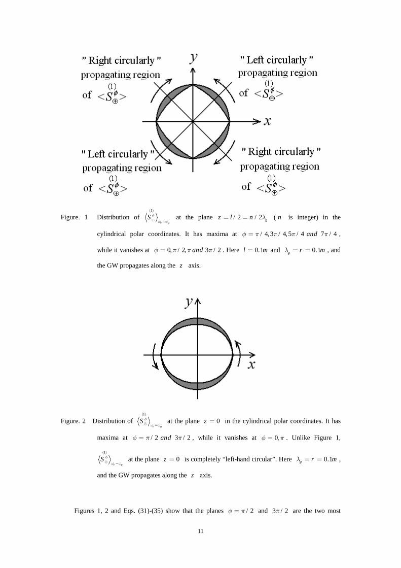
Figure. 1 Distribution of ( )1
e gS φ
ω ω⊕ =
0,φ π=
at the plane z l ( n is integer) in the
cylindrical polar coordinates. It has maxima at ,
while it vanishes at . Here and , and
the GW propagates along the axis.
/2 /2 gn λ= =
/4,φ π=
/2π 0.1l m=
3 ,5 / 4 7 /4andπ π
0.1g r mλ = =
/4π
/2, 3andπ
z
Figure. 2 Distribution of ( )1
e gS φ
ω ω⊗ =
/2=
at the plane in the cylindrical polar coordinates. It has
maxima at φ π , while it vanishes at φ . Unlike Figure 1,
0z =
3 /2and π 0,= π
( )1
e gS φ
ω ω⊗ = at the plane is completely “left-hand circular”. Here ,
and the GW propagates along the axis.
0z =
z
0.1g r mλ = =
Figures 1, 2 and Eqs. (31)-(35) show that the planes and 3 / are the two most /2φ π= 2π
11
interesting regions, in which ( ) ( )10
0e g
S Sφ φω ω⊕ =
= ≡ , but where ( ) ( )1 1
max|e g e g
S Sφ φω ω ω ω⊗ ⊗= =
=| | . This
means that any nonvanishing tangential EM power flux passing through the above surfaces will express
a pure EM perturbation produced by the HFGW.
|
C Numerical estimations
If we describe the perturbation in the quantum language (photon flux), the corresponding
perturbative photon flux n caused byφ
( )1
e gS φ
ω ω⊗ = at the surface (we note that /2φ π=
( )1
e gS φ
ω ω⊗ =is the unique nonvanishing power flux density passing through the surface) can be given
by
( )
( )0 0
1
1
, 20 / 2
1 ,e g
e g
w l
e e l
un S dzdr
φω ω φ
φ ω ω φ πω ω⊗ =
⊗ = =−
= = ∫ ∫ (36)
where ( ) ( )0 01 1
, 20 /2
e g e g
w l
l
u S dzdrφ φω ω ω ω φ π⊗ ⊗= = =
−
= ∫ ∫
/2φ π=
is the perturbative power flux passing through the
surface , is the Planck constant.
1. The electromagnetic response to the 3GH HFGW
In order to give reasonable estimation, we choose the achievable values of the EM parameters in
the present experiments: (1) , and 10 , respectively, the power of the Gaussian
beam. If the spot radius W of the Gaussian beam is limited in , then the power can be
estimated as
510P W=
0
310 W W
0.1m
( )0z
×
GH
0
0
W= ∫
1− 1.31
30 3gν =
02z rdπ=
3 110 Vm−
(0)ˆ 30yB =
z
P S [see Eq. (5)], the values of will be ,
and , respectively. The above power is well within the current
technology condition [6-8]. (2) , the strength of the background static magnetic field, this
is also achievable strength of a stationary magnetic field under the present experimental condition [14].
(3) , . Substituting Eqs. (33), (35) and the above parameters into Eq. (36), and
r 0ψ5 11.31 10 Vm−×
41.31 10 Vm×
10A −⊗ =
T
12
setting , , we obtain n s and
, respectively (see Table I). If the integration region of the radial coordinate in Eq. (36)
is moved to W r (where W m , ), in the same way, the corresponding
perturbative photon flux n can be estimated as
0 0.1W l m= =
10s−
0 ≤ ≤
0 0.3l =
0 0
m 3 14.75 10 ,φ−= ×
2m
2 14.75 10 s−×
r4.75 1×
r 0.1= 0 0.r =
φ′
( )0 0
0
1
/ 2e g
r l
e w l
S φω ω⊗
−∫ ∫
nφ′ <
0W
A
3 1s− 4.
( )
, / 24.dzdr
π≈
nφ′
( )g Hzν
1nφ ω′ = 46 10×
nφ n
φ= =
nφ
, and , respectively.
We can see that , but retains basically the same order of magnitude as , and because
then the “receiving surface” of the tangential photon flux has already moved to the region outside the
spot radius of the Gaussian beam, this result has more realistic meaning to distinguish and display
the perturbative photon flux.
2 146 10 s−× 4.46 110s−
nφ
×
φ′
P W( )1
( )e g
u Wφω ω⊗ =
φ ( )1− n sφ′n s
3010− 93 10× 510 200.95 10−× 4.75 310 4.46××3010−
3010−
93 10×93 10×
310 210.95 10−× 4.75220.95 10−× 4.
210 4.46×
10× 4.46
×
7510
nφ 0n ψ∝ ∝
110n s−
1.3THz
P
10
4.46nφ′ ≈ ×
eω =
φ′
4.75φ ≈ ×
P
nφ φ′(0)yn B∝
(0)yB
W
110 −
gω
1.3THz
Table I. The perturbative photon fluxes , , the power of the background Gaussian beam and
corresponding relevant parameters.
( )1−
(1) 310
(2) 210
(3) 10×
We emphasize that here , [see Eqs. (33)(35) and (36)], and at the same time,
, . Therefore, even if P is reduced to (this is already a very relaxed
requirement), we have still , (see Table I). Thus, if possible,
increasing (in this way the number of the background real photons does not change) has better
physical effect than increasing .
s
2. The electromagnetic response to the HFGW
According to the above discussions, it is easily to study the EM response to the HFGW.
Obviously, in this case the synchroresonance condition can be directly satisfied as long as
the frequency of the Gaussian beam is tuned to the . 1.3THz
13
In the same way, we list the power of the Gaussian beam, the perturbative power flux passing
through the surface (∼ ), the perturbative photon fluxes n , and the other
relevant parameters in Table II.
P
2m/2φ π= 210−φ nφ′
Table II. The perturbative photon fluxes , , the power of the background Gaussian beam and
corresponding relevant parameters.
nφ nφ′
A ( )g Hzν ( )P W ( )1
( )e g
u Wφω ω⊗ =
1( )n sφ− 1( )n sφ
−′
(1) 2810− 121.3 10× 510 181.46 10−× 31.69 10× 30.94 10×
(2) 2810− 121.3 10× 310 191.46 10−× 21.69 10× 20.94 10×
(3) 2810− 121.3 10× 10 201.46 10−× 1.69 10× 0.94 10×
-5 5 10 15 20 25 30zH×10−2mL250
500
750
1000
1250
1500
nφHs−1L
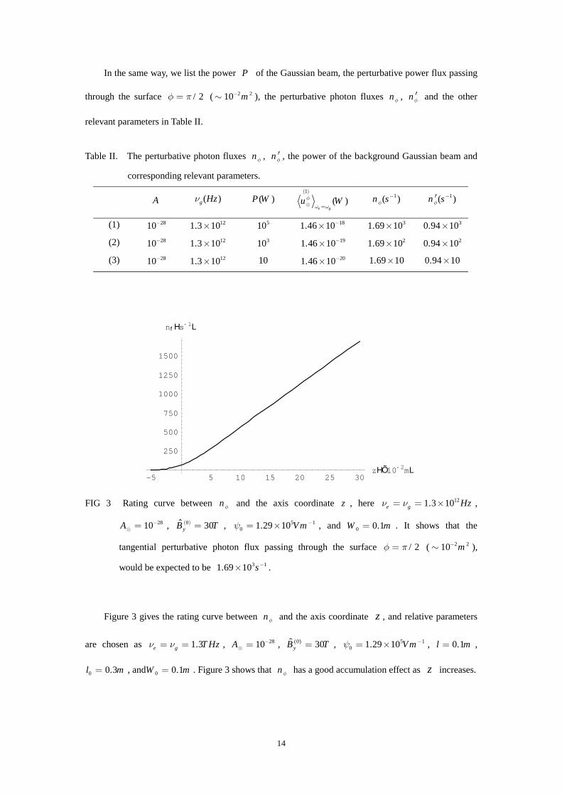
FIG 3 Rating curve between and the axis coordinate z , here ,
, , , and W . It shows that the
tangential perturbative photon flux passing through the surface φ π ( ∼ ),
would be expected to be .
nφ
1.69
121.3 10e g Hzν ν= = ×
1m
/2= 2 210 m−
2810A −⊗ =
( )0ˆ 30yB T= 50 1.29 10 Vmψ −= ×
3 110 s−×
10 0.=
Figure 3 gives the rating curve between and the axis coordinate nφ z , and relative parameters
are chosen as , , , , ,
, andW . Figure 3 shows that has a good accumulation effect as
1.3e g THzν ν= =
0 0.1m=
28−10A⊗ =(0)ˆ 30yB T=
φ
5 10 1. 10 Vmψ −29= × 0.1l m=
0 0.3l m= n z increases.
14

IV. NOISE ISSUES
Since in our EM system the response frequencies are much higher than ones of usual environment
noise sources (e.g., mechanical, seismic noise, etc.), the requirement of relevant conditions can be
further relaxed. Moreover, this EM system has the following advantages to reduce noise: (1) For the
possible external EM noise sources, the use of a Faraday cage or special fractal materials would be
very helpful. Once the EM system is isolated from the outside world by such means, the possible noise
sources would be the remaining thermal photons and self-background action. (2) Because of the
“random motion” of the remaining thermal photons and the highly directional propagated property of
the perturbative photon fluxes, the influence of such noise would be effectively suppressed in the local
regions. (3) Since the background photon fluxes vanish while the perturbative photon fluxes have
maxima in some special regions (e.g., the surfaces φ π and ), such that the
signal-to-noise ratio would be much larger than unity at these surfaces, although the background
photon fluxes are much greater than the perturbative photon fluxes in other regions. (4) Even if for the
mixed regions of the signal and the background action, because the self-background action would
decay as
/2= 3 /2φ π=
2
2
2exp rW
−
[see Eqs. (5)-(7)] while the signal (the perturbative photon fluxes) would decay
as 2
2
rW
−
W 4W
exp
3r =
[see Eqs. (34) and (35)], the signal-to-noise ratio may reach up to unity in the regions
of or , roughly. Of course, in such regions the signal will be reduced to a very small
value, but increasing background static field (if possible) may be a better way, because in this way the
number of the background real photons does not change. Besides, low-temperature vacuum operation
might effectively reduce the frequency of the remaining thermal photons and avoid dielectric
dissipation. Therefore, the crucial parameters for the noise problems are the selected perturbative
photon fluxes passing through the special surfaces and not the all background photons.
V A POSSIBLE JUXTAPOSED TEST SCHEME FOR THE ELECTROMAGNETIC
DETECTING SYSTEM AND THE HFGW GENERATORS
We shall consider the juxtaposed test scheme for our EM detecting system and 3GHz HFGW and
1.3THz HFGW generators.
Supposing that the EM detecting system is just laid at the optimal radiative direction, and the
15
HFGW in the wave zone can be seen as a quasi-plane GW (as we have pointed out in section III), then
the average power flux density of the HFGW of the × polarization state in the wave zone can be
estimated as
3 2
2 .32GWcS
Gωπ ⊗≈ A (37)
Thus the total power flux of the HFGW passing through the effective interaction region (cross
section) of the EM system will be
3 2
20( ) ( )
32GW GWcu S R A R
Gωπ ⊗= = 2
0 , (38)
where should be the same order of magnitude at least as the spot radius W of the Gaussian
beam.
0R 0
Using the first-order perturbative EM power flux (1)
e guφ
ω ω⊗ = and the effective power flux GWu
[see Eq.(38)] of the HFGW passing through the EM system, we can estimate “equivalent conversion
efficiency” of the HFGW to the perturbative EM power flux in our EM detecting system, which is
defined as
(1)
.e g
GW
u
u
φω ωη
⊗ == (39)
In Table III we list the “equivalent conversion efficiencies” for the 3GHz HFGW of
and the 1.3THz HFGW of h in the EM detection system, the power of the background
Gaussian beam is chosen as .
3010h −=
2810−=
10P W=
TABLE III The “equivalent conversion efficiencies” of the 3GHz HFGW, 1.3THz HFGW and the
corresponding relevant parameters.
A ( )g Hzν ( )GWu W (1)
( )e g
u Wφω ω⊗ =
η
(1) 3010− 93 10× 8~ 10− 22~ 10− 14~ 10−
(2) 2810− 121.3 10× ~ 10 20~ 10− 21~ 10−
Table III shows that the “equivalent conversion efficiency” of the 3GHz HFGW with
will be seven orders larger than that of the 1.3THz HFGW with , but the absolute value of
the perturbative EM power flux
3010h −=
2810h −=
(1)
e guφ
ω ω⊗ = produced by the latter will be two orders larger than that of
16

the former. Recently, Fontana and R. M. L. Baker, Jr. [5] proposed a more interesting scheme (F-B
scheme) in which it is possible to generate 1.3THz HFGW of 10 by the high-temperature
superconductor (HTSC) in the laboratory. If we assume further that whole such radiation power can be
almost concentrated in the optimal radiative direction, and a power flux density of can be
made in the EM detecting system, then corresponding amplitude order of the HFGW would be
. In Table IV we give the perturbative EM power fluxes and the corresponding perturbative
photon fluxes generated by the 1.3THz HFGW (F-B scheme) in our EM detecting system.
7W
710 Wm−2
2610−∼
n sφ−′
9.38×
1010−
TABLE IV The perturbative parameters produced by the 1.3THz FHGW generator (Fontana-Baker
scheme)
A ( )g Hzν ( )P W ( )1
( )e g
u Wφω ω⊗ =
1( )n sφ− 1( )
(1) 2610− 121.3 10× 510 161.46 10−× 51.69 10× 410
(2) 2610− 121.3 10× 310 171.46 10−× 41.69 10× 39.38 10×
(3) 2610− 121.3 10× 10 181.46 10−× 31.69 10× 29.38 10×
In particular, since n indicates the tangential perturbative photon flux passing through the
“receiving” surface (∼ ) outside the spot radius W of the Gaussian beam, and
even if is reduced to 10W, we have still (see scheme (3) in Table IV), our EM
system should be suitable to detect the 1.3THz HFGW expected by F-B scheme.
φ′
/2φ π= 2 210 m−0
P 3 110nφ−′ ≈ s
Recently, Chiao [1-3] proposed a quantum transducers scheme with very high conversion
efficiency for the HFGW and high-frequency EM waves. Under the extreme optimal condition, the
conversion efficiency of a dissipationless superconductor might approach unity. Of course, since the
noise and there exist unexplained residual microwave and far-infrared lost in the superconductors [1],
the actual conversion efficiency would be much less than unity. In order to improve effectively the
conversion efficiency, it is necessary to eliminate these microwave residual losses and to cool the
superconductor down extremely low temperatures, such as millikelvins. It is unclear yet that what is an
actual conversion efficiency for Chiao’s quantum superconductor transducers or others. We suppose
now that the power conversion efficiency of the 3GHz HFGW superconductor generators can reach up
to , and assume further that one tenth of the whole radiative power can be concentrated in the
effective receiver region of the EM detecting system. In this case we will be able to estimate the
17

quantitative relation between the input EM power in the HFGW generator and the “output”
power (i.e.,
emP
(1)
e guφ
ω ω⊗ =
( )GWP W
and , ) in the EM detecting system (see Table V). nφ
u W
nφ′
710−
510−
η
~ 10− /2
TABLE V The input power in the HFGW generator, the “output” power in the 3GHz HFGW
EM detector and relevant parameters.
3GHz
( )emP W 'η ( )GW A P (W) η (1)
e guφ
ω ω⊗ =(W)
1( )n sφ− 1'( )n sφ
−
410
1010−
610−
3010−
510 310
10
1310−
1410−
1510−
200.95 10−×210.95 10−×220.95 10−×
34.75 10× 24.75 10×
4.75 10×
34.46 10×24.46 10×
4.46 10×
610
1010−
410−
2910−
510 310
10
1410−
1510−
1610−
190.95 10−×200.95 10−×210.95 10−×
44.75 10× 34.75 10× 24.75 10×
44.46 10×34.46 10×24.46 10×
In Table V is the total input EM power in the 3GHz HFGW generator, is assumed the
power conversion efficiency from to in the superconducting generator, is the
effective HFGW power flux passing through to the EM detector, A is the dimensionless amplitude of
the HFGW, is the power of the Gaussian beam, is the “equivalent conversion efficiency” from
to
emP η ′
emP GWP GWu
P
GWu( )
ε
φω⊗
1
u= gω
in the EM detector, , are the corresponding perturbative photon fluxes. It
should be pointed out that in Table V only the power conversion efficiency η in the HFGW
generator is assumed, while other all calculations come out of the general theory of relativity of the
weak gravitational field and the electrodynamical equations in curved spacetime, and the chosen
parameters are well within the current technology conditions, or they are achievable values of the
present experimental possibilities.
nφ nφ′
′
We emphasize again that (1) since the highly directional propagated property of the perturbative
photon fluxes , and the “random motion” of the remained thermal photons, requirement for the
system’s temperature can be greatly relaxed. (2) and are unique nonvanishing photon fluxes
passing through the surface ( ) of φ π or . In this case any photon
measured from such photon fluxes at the above surfaces will be a signal of the EM perturbation
nφ nφ′
nφ
=
nφ′
2 2m 3 /2φ π=
18
produced by the HFGW in the GHz to THz band. (3) If we can find a very subtle means in which the
pure perturbative photon flux can be pumped out from our EM system, so that the perturbative and the
background photon fluxes can be completely separated, then the possibility of detecting the HFGW
would be greatly increased. More research into this subject remains to be done.
Acknowledgements
We are grateful to Dr. R. M. L. Baker, Jr. and Dr. P. A. Murad for their attention, helpful
suggestion to this manuscript and useful remarks.
This work is supported by the National Nature Science Foundation of China under Grants No.
10175096 and the Hubei Province Key Laboratory Foundation of Gravitational and Quantum Physics
under Grants No. GQ 0101.
References
[1] R. Y. Chiao (2002), gr-qc/0204012; gr-qc/0211078.
[2] A.. D. Speliotopuulos and R. Y. Chiao (2003), gr-qc/0302045.
[3] R. Y. Chiao and W. J. Fitelson (2003), gr-qc/0303089.
[4] R. M. L. Baker, Jr. (2003), “High-Frequency Gravitational Waves”, Max Plank Institute for
Astrophysics (MPA) Lecture, May.
[5] D. G. Fontana and R. M. L. Baker, Jr., (2003) “The High-Temperature Superconductor (HTSC)
Gravitational Laser (GASER)”. Paper HFGW-03-107 Gravitational-Wave Conference, The
MITRE Corporation, May 6-9.
[6] A. Modena et al. (1995), Nature (London) 337, 606.
[7] B. A. Remington et al. (1999), Science 284, 1488.
[8] M. Kushwah et al. (2002), Anode Modrlator Power Supplies For Continuous Duty 500KW
Klystrons (TH2103D) and 200KW Gyrotron (VGA8000A19), IEEE, Symposium on Fusion
Engineering. pp. 84-87.
[9] Fang-Yu Li and Meng-Xi Tang (2002), Int. J. Mod. Phys. D11, 1049.
[10] A. Yariv (1975), Quantum Electronics, 2nd ed. (Wiley, New York).
[11] Fand-Yu Li, Meng-Xi Tang, Jun Luo and Yi-Chuan. Li (2000), Phys. Rev. D 62, 044018.
[12] J. M. Condina et al. (1980), Phys. Rev. D 21, 2371.
[13] Fang-Yu Li, Meng-Xi Tang and Dong-Ping Shi (2003), “Electromagnetic Response of a Gaussian
Beam to High-Frequency Relic Gravitational Waves in Quintessential Inflationary Models”,
Chongqing University Report (2003); to be published in Phys. Rev. D67.
[14] G. Boebinger, A. Passner and J. Bevk (1995), Sci. Am. (Int. Ea) 272, 34.
19