Electromagnetic Generators for Portable Power Applications

by

Matthew Kurt Senesky

B.A. (Dartmouth College) 1998B.Eng. (Dartmouth College, Thayer School of Engineering) 1999

M.S. (University of California, Berkeley) 2003

A dissertation submitted in partial satisfaction of the

requirements for the degree of

Doctor of Philosophy

in

Engineering – Electrical Engineering and Computer Sciences

in the

GRADUATE DIVISION

of the

UNIVERSITY OF CALIFORNIA, BERKELEY

Committee in charge:Professor Seth R. Sanders, Chair

Professor Albert P. PisanoProfessor Dennis K. Lieu

Spring 2005

The dissertation of Matthew Kurt Senesky is approved:

Chair Date

Date

Date

University of California, Berkeley

Spring 2005

Electromagnetic Generators for Portable Power Applications

Copyright 2005

by

Matthew Kurt Senesky

1

Abstract

Electromagnetic Generators for Portable Power Applications

by

Matthew Kurt Senesky

Doctor of Philosophy in Engineering – Electrical Engineering and Computer

Sciences

University of California, Berkeley

Professor Seth R. Sanders, Chair

The power source that is common to almost all electrically powered portable devices

— the electrochemical battery — has failed to shrink at the same rate as circuits and

sensors. While this growing disparity has been partially mitigated by the decreas-

ing power requirements of many electronic circuits, the size and weight of portable

electronic devices are increasingly dominated by electrochemical batteries. An ob-

vious set of candidates for energy storage with higher levels of specific energy are

hydrocarbon fuels, long used in transportation applications for just this reason.

Several recent research efforts have sought to capitalize on the high specific energy

of chemical fuels through the use of MEMS engines or turbines paired with electrical

generators. Producing such a system to run efficiently on the milli- or microscale,

2

however, poses considerable challenges in thermal and fluid management, combustion

processes, and electromechanical energy conversion.

The contribution of the research presented in this dissertation is in the area of

electromechanical energy conversion. The design, construction and testing of an elec-

trical generator intended for interface with a MEMS–scale IC engine are presented.

The majority of the generator structure is built at the millimeter scale from discrete

parts, with only the rotor being microfabricated. We believe that this approach offers

superior performance as compared to purely microfabricated generators for power

outputs on the order of milliWatts and above, with only a modest penalty in mass

and volume.

Some of the design ideas from this millimeter scale generator are then extended

to the macro scale, with focus on a power range of tens to hundreds of Watts. The

application of interest is a generator for combustion-based portable power systems,

and hence power density is a key metric. However, there are an enormous number of

applications over a wide range of power levels — from implantable medical devices to

power tools to electric vehicle drives to wind power generation — that would benefit

from high-density motor or generator technology.

Professor Seth R. SandersDissertation Committee Chair

i

To my mother,

for passing her cleverness on to her children,

my father,

for teaching me the value of hard work through tireless example,

my sister,

for helping me to cope with the effects of cleverness and hard work,

and Debbie,

for seeing my qualities and ignoring my faults.

ii

Contents

List of Figures vi

List of Tables viii

1 Portable Power 1

1.1 Applications and Trends . . . . . . . . . . . . . . . . . . . . . . . . . 31.1.1 Consumer Electronics . . . . . . . . . . . . . . . . . . . . . . . 31.1.2 Military Applications . . . . . . . . . . . . . . . . . . . . . . . 41.1.3 Human Exoskeleton . . . . . . . . . . . . . . . . . . . . . . . . 51.1.4 Micro and Nano Air Vehicles . . . . . . . . . . . . . . . . . . . 51.1.5 Sensor Networks . . . . . . . . . . . . . . . . . . . . . . . . . 6

1.2 Technology . . . . . . . . . . . . . . . . . . . . . . . . . . . . . . . . 61.2.1 Energy Harvesting . . . . . . . . . . . . . . . . . . . . . . . . 61.2.2 Batteries . . . . . . . . . . . . . . . . . . . . . . . . . . . . . . 81.2.3 Fuel Cells . . . . . . . . . . . . . . . . . . . . . . . . . . . . . 91.2.4 Power MEMS . . . . . . . . . . . . . . . . . . . . . . . . . . . 12

1.3 The MEMS Rotary Engine Power System . . . . . . . . . . . . . . . 131.3.1 Concept . . . . . . . . . . . . . . . . . . . . . . . . . . . . . . 131.3.2 MEMS Wankel Engine . . . . . . . . . . . . . . . . . . . . . . 141.3.3 Generator . . . . . . . . . . . . . . . . . . . . . . . . . . . . . 141.3.4 Fluidic Systems . . . . . . . . . . . . . . . . . . . . . . . . . . 151.3.5 Packaging . . . . . . . . . . . . . . . . . . . . . . . . . . . . . 15

1.4 Scope of Research and Outline . . . . . . . . . . . . . . . . . . . . . . 16

2 Magnetic Properties of Materials 18

2.1 Material Properties . . . . . . . . . . . . . . . . . . . . . . . . . . . . 192.1.1 Soft Magnetic Materials . . . . . . . . . . . . . . . . . . . . . 222.1.2 Hard Magnetic Materials . . . . . . . . . . . . . . . . . . . . . 23

2.2 Temperature Effects . . . . . . . . . . . . . . . . . . . . . . . . . . . 282.3 Frequency Effects . . . . . . . . . . . . . . . . . . . . . . . . . . . . . 29

iii

2.3.1 Skin Effect at High Frequency . . . . . . . . . . . . . . . . . . 292.3.2 Losses in Soft Magnetic Materials . . . . . . . . . . . . . . . . 30

2.4 Magnetic Materials in MEMS . . . . . . . . . . . . . . . . . . . . . . 322.4.1 Fabrication Techniques . . . . . . . . . . . . . . . . . . . . . . 322.4.2 Soft Magnetic Materials for MEMS . . . . . . . . . . . . . . . 342.4.3 Hard Magnetic Materials for MEMS . . . . . . . . . . . . . . 35

3 Electric Machine Technology 38

3.1 Electric Machine Types . . . . . . . . . . . . . . . . . . . . . . . . . . 393.1.1 Reluctance . . . . . . . . . . . . . . . . . . . . . . . . . . . . 393.1.2 Electromagnetic Induction . . . . . . . . . . . . . . . . . . . 403.1.3 Permanent Magnet . . . . . . . . . . . . . . . . . . . . . . . . 413.1.4 Electrostatic . . . . . . . . . . . . . . . . . . . . . . . . . . . 42

3.2 Electric Machine Configurations . . . . . . . . . . . . . . . . . . . . . 423.2.1 Radial . . . . . . . . . . . . . . . . . . . . . . . . . . . . . . . 423.2.2 Axial . . . . . . . . . . . . . . . . . . . . . . . . . . . . . . . 433.2.3 Transverse . . . . . . . . . . . . . . . . . . . . . . . . . . . . 44

3.3 Scaling of Electromechanical Actuators . . . . . . . . . . . . . . . . . 453.3.1 Fundamental Limits . . . . . . . . . . . . . . . . . . . . . . . 453.3.2 Scaling of Electromagnetic Machines . . . . . . . . . . . . . . 473.3.3 Scaling Strategies . . . . . . . . . . . . . . . . . . . . . . . . 50

3.4 Survey of Small Electric Machines . . . . . . . . . . . . . . . . . . . . 513.4.1 Macro-Scale Machines . . . . . . . . . . . . . . . . . . . . . . 513.4.2 Microfabricated Machines . . . . . . . . . . . . . . . . . . . . 51

4 Analysis of Electromechanical Systems 54

4.1 Maxwell’s Equations . . . . . . . . . . . . . . . . . . . . . . . . . . . 554.1.1 Quasi-static Magnetic Equations . . . . . . . . . . . . . . . . 56

4.2 Magnetic Circuit Analysis . . . . . . . . . . . . . . . . . . . . . . . . 584.3 Energy Method Analysis . . . . . . . . . . . . . . . . . . . . . . . . . 60

4.3.1 Calculations Using the Energy Method . . . . . . . . . . . . . 614.3.2 Energy Versus Coenergy . . . . . . . . . . . . . . . . . . . . . 644.3.3 Treatment of Permanent Magnets . . . . . . . . . . . . . . . . 664.3.4 Treatment of Multiple Windings . . . . . . . . . . . . . . . . . 684.3.5 The Energy Method for Distributed Fields . . . . . . . . . . . 69

4.4 Finite Element Analysis . . . . . . . . . . . . . . . . . . . . . . . . . 714.4.1 Calculation of the Finite Element Solution . . . . . . . . . . . 724.4.2 Force Calculations . . . . . . . . . . . . . . . . . . . . . . . . 73

4.5 A Comparison of Various Analysis Methods . . . . . . . . . . . . . . 744.5.1 Field Quantities . . . . . . . . . . . . . . . . . . . . . . . . . . 754.5.2 Magnetic Circuit Analysis . . . . . . . . . . . . . . . . . . . . 774.5.3 Coenergy Calculation Via Fictitious Winding . . . . . . . . . 78

iv

4.5.4 Coenergy Calculation Via Equivalent Winding . . . . . . . . . 794.5.5 Coenergy Calculation Via Coenergy Density . . . . . . . . . . 794.5.6 Equivalence of Lumped Element and Field Calculation . . . . 80

5 Machine Design and Analysis — Millimeter Scale 83

5.1 Design . . . . . . . . . . . . . . . . . . . . . . . . . . . . . . . . . . . 835.2 Analysis . . . . . . . . . . . . . . . . . . . . . . . . . . . . . . . . . . 865.3 Construction . . . . . . . . . . . . . . . . . . . . . . . . . . . . . . . 935.4 Results . . . . . . . . . . . . . . . . . . . . . . . . . . . . . . . . . . . 97

5.4.1 Torque . . . . . . . . . . . . . . . . . . . . . . . . . . . . . . . 975.4.2 Open-Circuit Voltage and Power . . . . . . . . . . . . . . . . 100

6 Machine Design and Analysis — Centimeter Scale 103

6.1 Rationale . . . . . . . . . . . . . . . . . . . . . . . . . . . . . . . . . 1046.2 Design . . . . . . . . . . . . . . . . . . . . . . . . . . . . . . . . . . . 106

6.2.1 Stator . . . . . . . . . . . . . . . . . . . . . . . . . . . . . . . 1086.2.2 Rotor . . . . . . . . . . . . . . . . . . . . . . . . . . . . . . . 109

6.3 Analysis . . . . . . . . . . . . . . . . . . . . . . . . . . . . . . . . . . 1136.3.1 Lumped-Element Model . . . . . . . . . . . . . . . . . . . . . 1136.3.2 Monte Carlo Optimization . . . . . . . . . . . . . . . . . . . . 1166.3.3 Finite-Element Analysis . . . . . . . . . . . . . . . . . . . . . 121

7 Conclusions 127

7.1 Thoughts on Millimeter-Scale Design . . . . . . . . . . . . . . . . . . 1277.2 Thoughts on Centimeter-Scale Design . . . . . . . . . . . . . . . . . . 1297.3 Thoughts on Future Research Directions . . . . . . . . . . . . . . . . 130

7.3.1 Isotropic Materials . . . . . . . . . . . . . . . . . . . . . . . . 1317.3.2 Small Gap, Low Speed Machine . . . . . . . . . . . . . . . . . 1317.3.3 Materials and Manufacturing . . . . . . . . . . . . . . . . . . 132

Bibliography 134

A Equations 141

A.1 Magnetic Circuit Equations . . . . . . . . . . . . . . . . . . . . . . . 141A.2 Combining FEA Results at Varying Radius . . . . . . . . . . . . . . . 143A.3 Coenergy Density in Nonlinear Materials . . . . . . . . . . . . . . . . 144

B Material Data 147

C Simulation Code 151

C.1 Lumped Element Calculations . . . . . . . . . . . . . . . . . . . . . . 151C.2 Monte-Carlo Optimization . . . . . . . . . . . . . . . . . . . . . . . . 154C.3 Finite Element Analysis . . . . . . . . . . . . . . . . . . . . . . . . . 158

v

D Mechanical Drawings 168

D.1 Millimeter-Scale Generator Components . . . . . . . . . . . . . . . . 168

vi

List of Figures

1.1 Notebook computer and cellular handset usage . . . . . . . . . . . . . 4

2.1 Typical family of B-H loops . . . . . . . . . . . . . . . . . . . . . . . 202.2 Typical soft magnetic B-H characteristic . . . . . . . . . . . . . . . . 222.3 Typical hard magnetic B-H characteristic . . . . . . . . . . . . . . . . 242.4 Core loss density of silicon steel laminations and powdered iron . . . 32

3.1 Radial flux machine configuration . . . . . . . . . . . . . . . . . . . . 433.2 Axial flux machine configuration . . . . . . . . . . . . . . . . . . . . . 433.3 Transverse flux machine configuration . . . . . . . . . . . . . . . . . . 443.4 Paschen’s curve for electrostatic breakdown . . . . . . . . . . . . . . . 46

4.1 A simple magnetic circuit . . . . . . . . . . . . . . . . . . . . . . . . 584.2 Conceptual electromechanical actuator . . . . . . . . . . . . . . . . . 614.3 Relationship between flux, current, energy and coenergy . . . . . . . 654.4 Change in energy and coenergy resulting from a change in displacement 664.5 Test structure for electromagnetic analysis . . . . . . . . . . . . . . . 754.6 Graphical depiction of field quantities in test structure . . . . . . . . 764.7 Magnetic circuit model of test structure . . . . . . . . . . . . . . . . . 774.8 Graphical depiction of terminal quantities of test structure . . . . . . 814.9 Coenergy versus displacement of test structure . . . . . . . . . . . . . 824.10 Force versus displacement of test structure . . . . . . . . . . . . . . . 82

5.1 Millimeter-scale generator assembly . . . . . . . . . . . . . . . . . . . 845.2 Millimeter-scale generator schematic cross-section . . . . . . . . . . . 855.3 Microfabricated Wankel rotor . . . . . . . . . . . . . . . . . . . . . . 865.4 Magnetic circuit model of millimeter-scale generator . . . . . . . . . . 875.5 Simplified magnetic circuit model for millimeter-scale generator . . . 875.6 Pole area parameter definitions for magnetic circuit model . . . . . . 895.7 Length parameter definitions for magnetic circuit model . . . . . . . . 895.8 Axisymmetric finite element models of millimeter-scale generator . . . 93

vii

5.9 Millimeter-scale generator prototype . . . . . . . . . . . . . . . . . . 945.10 Powdered iron stator pole faces . . . . . . . . . . . . . . . . . . . . . 955.11 Laminated silicon steel center post . . . . . . . . . . . . . . . . . . . 955.12 Electroplated rotor . . . . . . . . . . . . . . . . . . . . . . . . . . . . 965.13 B-H characteristic of electroplated NiFe material . . . . . . . . . . . . 965.14 Laminated silicon steel toroid . . . . . . . . . . . . . . . . . . . . . . 975.15 Steel test rotor for millimeter-scale generator . . . . . . . . . . . . . . 975.16 Torque experiment setup . . . . . . . . . . . . . . . . . . . . . . . . . 985.17 Generator open circuit output voltage . . . . . . . . . . . . . . . . . . 1025.18 Generator average power output versus load resistance . . . . . . . . 102

6.1 Macro-scale generator design concept . . . . . . . . . . . . . . . . . . 1076.2 Macro-scale generator stator detail . . . . . . . . . . . . . . . . . . . 1086.3 Macro-scale generator pole face configuration . . . . . . . . . . . . . . 1086.4 Surface magnet rotor . . . . . . . . . . . . . . . . . . . . . . . . . . . 1116.5 Embedded magnet rotor . . . . . . . . . . . . . . . . . . . . . . . . . 1116.6 Back-to-back Halbach array rotor . . . . . . . . . . . . . . . . . . . . 1116.7 Gap flux density for surface magnet rotor . . . . . . . . . . . . . . . . 1116.8 Gap flux density for embedded magnet rotor . . . . . . . . . . . . . . 1116.9 Gap flux density for Halbach array rotor . . . . . . . . . . . . . . . . 1116.10 Conceptual magnetic structure of macro-scale generator . . . . . . . . 1146.11 Magnetic circuit model of macro-scale generator . . . . . . . . . . . . 1146.12 Monte Carlo optimization results for macro-scale generator . . . . . . 1196.13 Monte Carlo result for power output versus outer radius . . . . . . . 1206.14 Monte Carlo result for efficiency versus outer radius . . . . . . . . . . 1206.15 Finite-element model of macro-scale generator . . . . . . . . . . . . . 1246.16 Typical finite-element solution for macro-scale generator . . . . . . . 1246.17 Flux linkage versus rotor angle from magnetic circuit and FEA . . . . 1256.18 Coenergy versus rotor angle calculated from magnetic circuit and FEA 1256.19 Torque versus rotor angle, calculated with magnetic circuit and FEA 126

B.1 Magnetization curve for Arnon 5 material . . . . . . . . . . . . . . . 147B.2 Core loss for Arnon 5 material . . . . . . . . . . . . . . . . . . . . . . 148B.3 B-H loop for Micrometals -26 material . . . . . . . . . . . . . . . . . 149B.4 Permeability versus field intensity for Micrometals -26 material . . . . 150

viii

List of Tables

1.1 Various classes of sensor nodes . . . . . . . . . . . . . . . . . . . . . . 71.2 Primary battery data . . . . . . . . . . . . . . . . . . . . . . . . . . . 91.3 Secondary battery data . . . . . . . . . . . . . . . . . . . . . . . . . . 101.4 Chemical fuel data . . . . . . . . . . . . . . . . . . . . . . . . . . . . 13

2.1 Magnetic material designations . . . . . . . . . . . . . . . . . . . . . 192.2 Soft magnetic material properties . . . . . . . . . . . . . . . . . . . . 232.3 Hard magnetic material properties . . . . . . . . . . . . . . . . . . . . 272.4 Curie point of selected magnetic materials . . . . . . . . . . . . . . . 282.5 Skin depths of selected materials at 500 Hz . . . . . . . . . . . . . . . 30

3.1 Comparison of electric machine technologies . . . . . . . . . . . . . . 423.2 Specifications of selected off-the-shelf BLDC machines . . . . . . . . . 52

4.1 Comparison of electric and magnetic circuit quantities . . . . . . . . . 60

5.1 Experimental results for millimeter-scale generator . . . . . . . . . . . 101

6.1 Fixed values and parameter ranges for Monte Carlo optimization . . . 1176.2 Design values chosen from Monte Carlo optimization results . . . . . 1216.3 Machine performance calculated from magnetic circuit results . . . . 121

ix

Acknowledgments

I’d like to thank foremost Seth Sanders, for his patient guidance and instruction,

optimistic nature, and willingness to entertain new ideas. I’d also like to thank Al

Pisano, for developing the compelling idea behind the MEMS REPS project, for his

input to my research, and for his heroic efforts to secure funding for many hungry

students. Dave Walther contributed many insights to my efforts as well, both technical

and humorous. I’d like to thank all the other members of the MEMS REPS team,

particularly Aaron Knobloch, Debbie Jones, and Fabian Martinez for their work in

adapting the Wankel rotor to my magnetic demands. Finally, I’d like to thank my

friends and family, for their love and support.

1

Chapter 1

Portable Power

We have made progress in the manufacturing of small things. Moore’s law has

held, miraculously, since it was posed in 1965; the number of transistors that can fit

on a microchip doubles approximately every 12-18 months. Over the last 15-20 years,

the field of MEMS — microelectromechanical systems — has grown from a laboratory

curiosity into an area of intense research and commercial opportunity. We reap the

benefits of these and other technological advancements every day, with the use of

increasingly convenient, increasingly commonplace and increasingly small portable

electronic devices.

However, a bottleneck looms on the horizon. The power source that is common to

almost all electrically powered portable applications — the electrochemical battery

— has failed to shrink at the same rate as circuits and sensors. While this disparity

has been partially mitigated by the decreasing power requirements of many electronic

2

circuits, the size and weight of portable electronic devices are increasingly dominated

by electrochemical batteries.

For applications such as cellular telephones and laptop computers, the size of bat-

teries has thus far been a manageable problem. The robust sales of these devices attest

to the fact that consumers find them relatively convenient. By the same measure,

however, a huge commercial windfall is available to the inventor of a cost-effective

technology to improve on the energy storage capability of state of the art batteries. In

a competitive marketplace, portable electronic products with the increased run-time

or increased functionality provided by an improved power source will be extremely

attractive to consumers.

Beyond the consumer market, there exist a large number of applications for which

even the best batteries are unsatisfactory. These include the most demanding military

applications, for which relatively high power levels are expected over mission lengths

that far exceed consumer demands, and sensor networks, which draw low levels of

power but require extremely high energy storage densities to achieve truly ubiquitous

application.

The remainder of this chapter will present some of the more compelling applica-

tions of small-scale power sources, followed by an overview of proposed technology

solutions.

3

1.1 Applications and Trends

1.1.1 Consumer Electronics

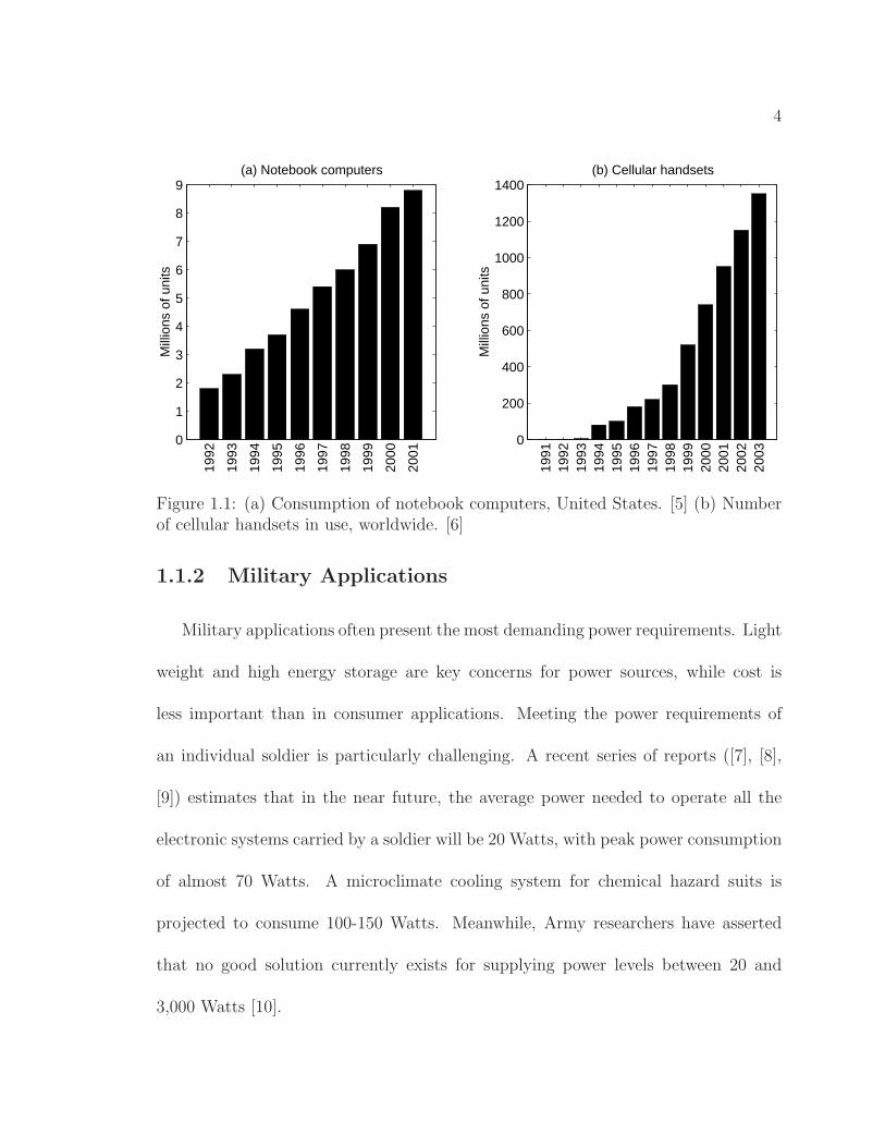
Cellular telephones and notebook computers have both experienced a boom in

popularity in the last decade. Between 1992 and 2001, sales of notebook computers

in the United States increased almost five-fold, reaching 8.8 million units in 2001

(Fig. 1.1a). Cellular telephones have shown an even more dramatic proliferation,

with units in use worldwide increasing from 1 million in 1991 to 1.35 billion in 2003

(Fig. 1.1b).

The power requirements of both notebook computers and cellular telephones are

currently met by lithium-ion (Li-Ion) batteries. A notebook computer in active oper-

ation can use power on the order of tens of Watts, while a cellular telephone in talk

mode may use on the order of a few Watts. The batteries in both devices are sized

so as to give the user about 4 hours of active operation.

For both types of device, the battery makes up a large fraction of the overall

mass, particularly for the smallest products. One of the smallest available cellular

phones, the Ericsson T66, has an overall mass of 59 grams, with a battery mass of

20 grams. Thus the battery represents more than one third of the total mass [1],[2].

A lightweight notebook computer, the Dell Latitude X300, has a mass of 1.32 kg,

to which the battery contributes 0.45 kg. Again the battery makes up just over one

third of the total mass [3],[4].

4

0

1

2

3

4

5

6

7

8

9(a) Notebook computers

Mill

ions

of u

nits

1992

1993

1994

1995

1996

1997

1998

1999

2000

2001

0

200

400

600

800

1000

1200

1400(b) Cellular handsets

Mill

ions

of u

nits

1991

19

92

1993

19

94

1995

19

96

1997

19

98

1999

20

00

2001

20

02

2003

Figure 1.1: (a) Consumption of notebook computers, United States. [5] (b) Numberof cellular handsets in use, worldwide. [6]

1.1.2 Military Applications

Military applications often present the most demanding power requirements. Light

weight and high energy storage are key concerns for power sources, while cost is

less important than in consumer applications. Meeting the power requirements of

an individual soldier is particularly challenging. A recent series of reports ([7], [8],

[9]) estimates that in the near future, the average power needed to operate all the

electronic systems carried by a soldier will be 20 Watts, with peak power consumption

of almost 70 Watts. A microclimate cooling system for chemical hazard suits is

projected to consume 100-150 Watts. Meanwhile, Army researchers have asserted

that no good solution currently exists for supplying power levels between 20 and

3,000 Watts [10].

5

1.1.3 Human Exoskeleton

Human exoskeletons are currently under investigation as a means of enhancing

the mechanical performance of the human body. By means of wearable mechanical

elements that supplement the force producing capability of the major muscle groups,

the user’s productivity could be enhanced in a warehouse or construction setting, or

in a military environment.

Researchers have estimated that the act of walking (4.5 mph), for a combined

exoskeleton and payload of 350 pounds, requires 310 Watts. If, in addition to walking,

a 100 lb. payload is lifted at 1 ft/s, power demand rises to 440 W. The act of running

(6.7 mph), again with an overall weight of 350 lbs. but with no lifting, is estimated

to consume 600 W in steady-state, with peak power requirements for rapid motions

reaching up to 2 kW [11].

1.1.4 Micro and Nano Air Vehicles

Several research efforts have recently created startlingly small flying vehicles.

Fixed wing [12], rotary wing [13], and flapping wing craft have all been demonstrated

with varying levels of success. It has been estimated that the minimum power re-

quired to keep a 50 gram MAV aloft is 600 mW [14]. The 80 gram fixed wing vehicle

described in [12] draws 4.35 W for propulsion, while the 12.3 gram rotary wing craft

in [13] draws 3.5 W.

6

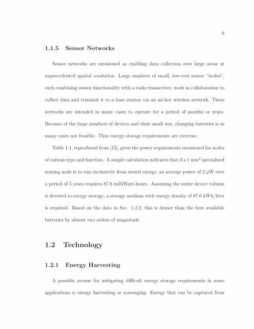
1.1.5 Sensor Networks

Sensor networks are envisioned as enabling data collection over large areas at

unprecedented spatial resolution. Large numbers of small, low-cost sensor “nodes”,

each combining sensor functionality with a radio transceiver, work in collaboration to

collect data and transmit it to a base station via an ad-hoc wireless network. These

networks are intended in many cases to operate for a period of months or years.

Because of the large numbers of devices and their small size, changing batteries is in

many cases not feasible. Thus energy storage requirements are extreme.

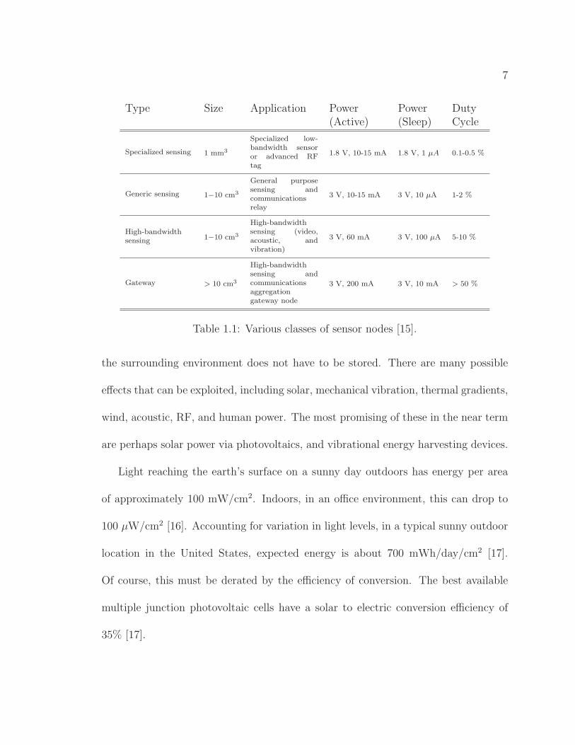
Table 1.1, reproduced from [15], gives the power requirements envisioned for nodes

of various type and function. A simple calculation indicates that if a 1 mm3 specialized

sensing node is to run exclusively from stored energy, an average power of 2 µW over

a period of 5 years requires 87.6 milliWatt-hours. Assuming the entire device volume

is devoted to energy storage, a storage medium with energy density of 87.6 kWh/liter

is required. Based on the data in Sec. 1.2.2, this is denser than the best available

batteries by almost two orders of magnitude.

1.2 Technology

1.2.1 Energy Harvesting

A possible avenue for mitigating difficult energy storage requirements in some

applications is energy harvesting or scavenging. Energy that can be captured from

7

Type Size Application Power Power Duty(Active) (Sleep) Cycle

Specialized sensing 1 mm3

Specialized low-bandwidth sensoror advanced RFtag

1.8 V, 10-15 mA 1.8 V, 1 µA 0.1-0.5 %

Generic sensing 1−10 cm3

General purposesensing andcommunicationsrelay

3 V, 10-15 mA 3 V, 10 µA 1-2 %

High-bandwidthsensing 1−10 cm3

High-bandwidthsensing (video,acoustic, andvibration)

3 V, 60 mA 3 V, 100 µA 5-10 %

Gateway > 10 cm3

High-bandwidthsensing andcommunicationsaggregationgateway node

3 V, 200 mA 3 V, 10 mA > 50 %

Table 1.1: Various classes of sensor nodes [15].

the surrounding environment does not have to be stored. There are many possible

effects that can be exploited, including solar, mechanical vibration, thermal gradients,

wind, acoustic, RF, and human power. The most promising of these in the near term

are perhaps solar power via photovoltaics, and vibrational energy harvesting devices.

Light reaching the earth’s surface on a sunny day outdoors has energy per area

of approximately 100 mW/cm2. Indoors, in an office environment, this can drop to

100 µW/cm2 [16]. Accounting for variation in light levels, in a typical sunny outdoor

location in the United States, expected energy is about 700 mWh/day/cm2 [17].

Of course, this must be derated by the efficiency of conversion. The best available

multiple junction photovoltaic cells have a solar to electric conversion efficiency of

35% [17].

8

Vibrational energy harvesting is typically accomplished with a proof mass mounted

on a spring element, coupled to an electromechanical transducer. Electromagnetic

[18], electrostatic [19], and piezoelectric [20] transducers have all been attempted.

The harvesting of vibrational energy is best suited to applications where the device

can be mounted to a rigid, vibrating body, and frequencies of vibration are well-

characterized. Uncertain placement, dissipative substrates, or frequencies far from

the device resonance can adversely affect performance.

1.2.2 Batteries

Electrochemical batteries are by far the dominant technology for portable power

applications. Of commercially available battery types, lithium–thionyl chloride (Li–

SOCl2) has the highest specific energy among primary batteries at present (660

Wh/kg), while lithium–sulfur (Li–S) leads among secondary batteries (370 Wh/kg)

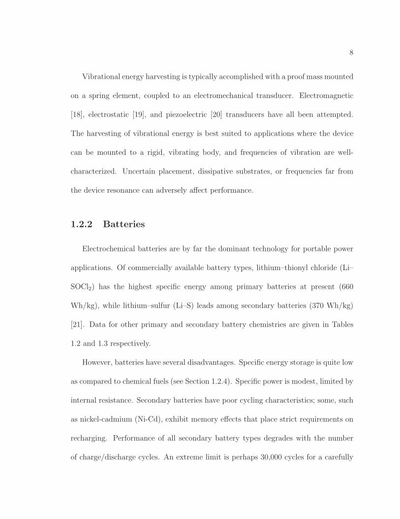
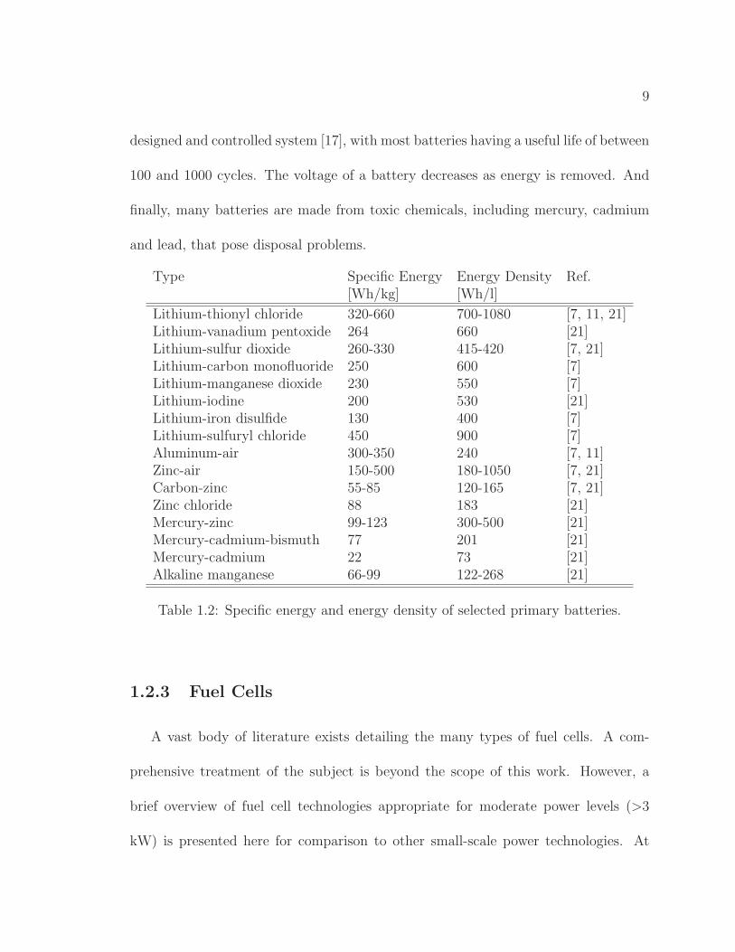
[21]. Data for other primary and secondary battery chemistries are given in Tables

1.2 and 1.3 respectively.

However, batteries have several disadvantages. Specific energy storage is quite low

as compared to chemical fuels (see Section 1.2.4). Specific power is modest, limited by

internal resistance. Secondary batteries have poor cycling characteristics; some, such

as nickel-cadmium (Ni-Cd), exhibit memory effects that place strict requirements on

recharging. Performance of all secondary battery types degrades with the number

of charge/discharge cycles. An extreme limit is perhaps 30,000 cycles for a carefully

9

designed and controlled system [17], with most batteries having a useful life of between

100 and 1000 cycles. The voltage of a battery decreases as energy is removed. And

finally, many batteries are made from toxic chemicals, including mercury, cadmium

and lead, that pose disposal problems.

Type Specific Energy Energy Density Ref.[Wh/kg] [Wh/l]

Lithium-thionyl chloride 320-660 700-1080 [7, 11, 21]Lithium-vanadium pentoxide 264 660 [21]Lithium-sulfur dioxide 260-330 415-420 [7, 21]Lithium-carbon monofluoride 250 600 [7]Lithium-manganese dioxide 230 550 [7]Lithium-iodine 200 530 [21]Lithium-iron disulfide 130 400 [7]Lithium-sulfuryl chloride 450 900 [7]Aluminum-air 300-350 240 [7, 11]Zinc-air 150-500 180-1050 [7, 21]Carbon-zinc 55-85 120-165 [7, 21]Zinc chloride 88 183 [21]Mercury-zinc 99-123 300-500 [21]Mercury-cadmium-bismuth 77 201 [21]Mercury-cadmium 22 73 [21]Alkaline manganese 66-99 122-268 [21]

Table 1.2: Specific energy and energy density of selected primary batteries.

1.2.3 Fuel Cells

A vast body of literature exists detailing the many types of fuel cells. A com-

prehensive treatment of the subject is beyond the scope of this work. However, a

brief overview of fuel cell technologies appropriate for moderate power levels (>3

kW) is presented here for comparison to other small-scale power technologies. At

10

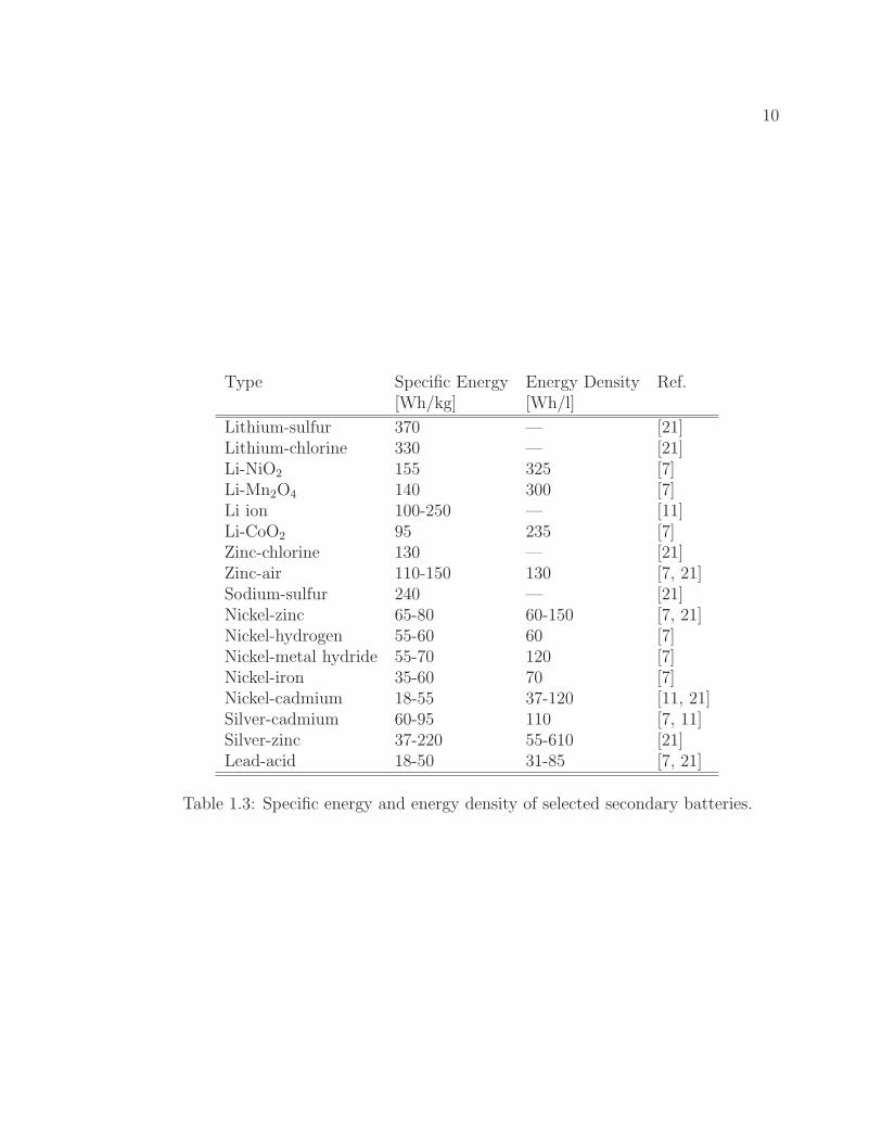
Type Specific Energy Energy Density Ref.[Wh/kg] [Wh/l]

Lithium-sulfur 370 — [21]Lithium-chlorine 330 — [21]Li-NiO2 155 325 [7]Li-Mn2O4 140 300 [7]Li ion 100-250 — [11]Li-CoO2 95 235 [7]Zinc-chlorine 130 — [21]Zinc-air 110-150 130 [7, 21]Sodium-sulfur 240 — [21]Nickel-zinc 65-80 60-150 [7, 21]Nickel-hydrogen 55-60 60 [7]Nickel-metal hydride 55-70 120 [7]Nickel-iron 35-60 70 [7]Nickel-cadmium 18-55 37-120 [11, 21]Silver-cadmium 60-95 110 [7, 11]Silver-zinc 37-220 55-610 [21]Lead-acid 18-50 31-85 [7, 21]

Table 1.3: Specific energy and energy density of selected secondary batteries.

11

present, proton exchange membrane fuel cells (PEMFCs), direct methanol fuel cells

(DMFCs), and formic acid fuel cells (FAFCs) are leading candidates for portable fuel

cell technology.

Polymer electrolyte membrane fuel cells oxidize pure hydrogen, and allow the

protons to pass through a membrane. The electrons pass through the load circuit,

delivering power. Because the protons recombine with oxygen at the other side of the

membrane, water is the only byproduct of the reaction. PEMFCs can reach efficiencies

of up to 60%, and specific power of approximately 1 kW/kg [9]. The technology has

yet to see widespread use, however, because of several drawbacks. The storage of

compressed hydrogen fuel presents the danger of explosion; the required containment

vessels significantly increase system mass. The fuel cell membrane can be poisoned

by small amounts of carbon monoxide (CO), requiring clean hydrogen sources. And

it is necessary to precisely regulate the amount of water in the system, adding to the

balance-of-plant (BOP).

Direct methanol fuel cells are similar to PEMFCs in construction, typically using

the same membrane and cathode catalyst. Methanol presents less danger than hy-

drogen of sudden explosion, and hence DMFCs do away with ponderous containment

vessels. However, a less efficient catalyst reaction reduces efficiency to approximately

40% [8]. Power density is modest at 0.2 W/kg [9]. DMFCs suffer from the same poi-

soning and water management problems as PEMFCs, with the additional problem

12

of methanol crossover — leakage of unreacted fuel across the membrane — which

further complicates the BOP and reduces practical efficiency.

A relatively recent development is the formic acid fuel cell [22]. Formic acid is

the toxin secreted by black ants; its high acidity is a drawback for use around human

operators. Further, formic acid has less than half the energy density of methanol

(see Table 1.4). FAFCs can operate with higher fuel concentrations than DMFCs

however, and can do so at ambient temperature. A FAFC has been presented ([23])

that achieves an area-wise power density of 110 mW/cm2.

1.2.4 Power MEMS

An obvious set of candidates for energy storage with higher levels of specific energy

are hydrocarbon fuels, long used in transportation applications for just this reason.

Gasoline, as shown in Table 1.4, has specific energy of 12.2 kWh/kg, roughly 18 times

that of Li–SOCl2 batteries and 33 times that of Li–S batteries; the more appropriate

comparison is with the primary technology however. Of course, chemical to thermal,

thermal to mechanical, and mechanical to electrical conversion efficiencies must be

taken into account in considering hydrocarbon fuels. However, a 10% overall conver-

sion efficiency still results in a higher specific energy than the best available primary

batteries.

Several recent research efforts have sought to capitalize on the high specific energy

of chemical fuels through the use of MEMS engines or turbines paired with electrical

13

generators [24], [25]. Producing such a system to run efficiently on the milli- or

microscale, however, poses considerable challenges in thermal and fluid management,

combustion processes, and electromechanical energy conversion.

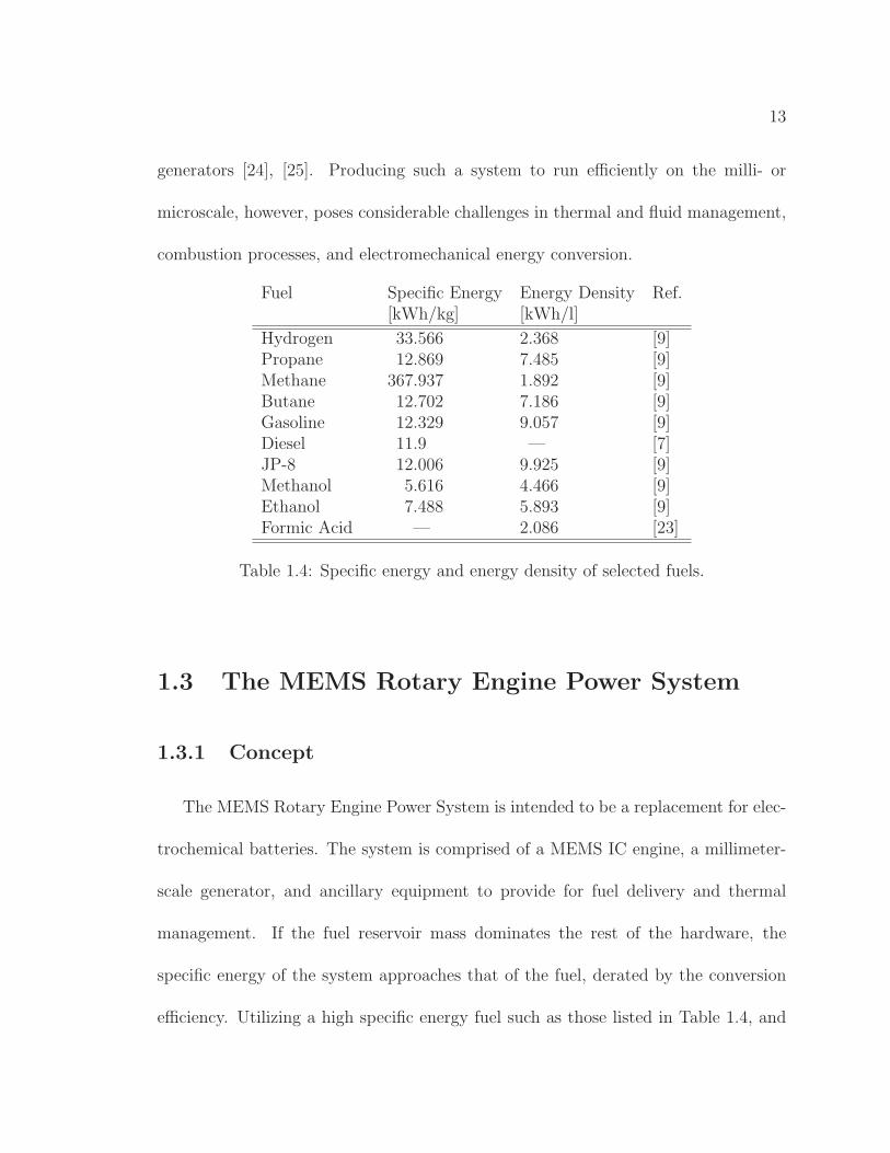
Fuel Specific Energy Energy Density Ref.[kWh/kg] [kWh/l]

Hydrogen 33.566 2.368 [9]Propane 12.869 7.485 [9]Methane 367.937 1.892 [9]Butane 12.702 7.186 [9]Gasoline 12.329 9.057 [9]Diesel 11.9 — [7]JP-8 12.006 9.925 [9]Methanol 5.616 4.466 [9]Ethanol 7.488 5.893 [9]Formic Acid — 2.086 [23]

Table 1.4: Specific energy and energy density of selected fuels.

1.3 The MEMS Rotary Engine Power System

1.3.1 Concept

The MEMS Rotary Engine Power System is intended to be a replacement for elec-

trochemical batteries. The system is comprised of a MEMS IC engine, a millimeter-

scale generator, and ancillary equipment to provide for fuel delivery and thermal

management. If the fuel reservoir mass dominates the rest of the hardware, the

specific energy of the system approaches that of the fuel, derated by the conversion

efficiency. Utilizing a high specific energy fuel such as those listed in Table 1.4, and

14

assuming moderate conversion efficiencies, the overall system mass can be smaller

than that of a battery of equivalent energy storage.

1.3.2 MEMS Wankel Engine

The IC engine to be used in the system is a microfabricated Wankel engine. The

Wankel engine has several advantages for such an application: it is inherently planar,

making it amenable to microfabrication; it is self-valving, reducing the number of

parts and complexity of the design; and like diesel engines, it can burn a wide range

of fuels. Sealing is a known problem of Wankel engines, and this problem can become

more severe at small scales as relative tolerances become worse.

The engine is fabricated with a deep reactive ion etch process [26, 27]; it consists

of a housing, shaft and rotor. The rotor is the most sophisticated component, having

electroplated nickel-iron poles [28], as well as integrated cantilever tip seals [29].

1.3.3 Generator

One of the contributions of the research presented in this dissertation is in the

design, construction and testing of an electrical generator intended for interface with

a MEMS–scale IC engine. The majority of the generator structure is built at the

millimeter scale from discrete parts, with only the rotor being microfabricated. We

believe that this approach offers superior performance as compared to purely micro-

15

fabricated generators for power outputs on the order of milliWatts and above, with

only a modest penalty in mass and volume.

The engine and generator are integrated into a single unit by mounting the genera-

tor stator to the silicon engine housing, and utilizing the engine rotor as the generator

rotor. This is achieved by electroplating nickel–iron (NiFe) poles into the rotor tips.

Integration of the engine and generator avoids shaft coupling between the two ma-

chines, simplifying assembly of the devices as well as improving sealing of the engine

housing and reducing unwanted heat flow out of the combustion chamber. It also,

however, places unique constraints on the generator design as detailed in Chapter 5.

1.3.4 Fluidic Systems

The delivery of fuel to the engine is a nontrivial problem. A precise fuel-air mixture

must flow to the combustion chamber under a wide range of operating conditions.

Further, the system that performs this function must use only a small fraction of

the engine output power. One possibility is to use the phase eruption of fuel in a

microchannel positioned to absorb waste heat from the engine. This approach is

explored in [30].

1.3.5 Packaging

As the dimensions of the engine shrink, its surface area to volume ratio increases,

and heat dissipates more quickly than at larger scales. In a cold engine, quenching

16

of the combustion flame can occur at the wall of the combustion chamber, causing

a loss of power. Thus, micro-scale engines need thermal insulation to maintain an

appropriate temperature, unlike macro-scale engines which need to be cooled.

The generator, however, experiences a decrease in performance as temperature

rises; soft magnetic permeability and saturation induction decrease, and hard mag-

netic residual flux density decreases. Hence a thermal package was created with the

goal of insulating the engine while providing cooling for the generator. This is ac-

complished through the use of aerogel insulation, which surrounds the engine housing

including the small gap between the housing and the generator stator. The stator,

meanwhile, is mounted directly to the metal package case, which allows heat to escape

to the outside.

1.4 Scope of Research and Outline

The remainder of this work concerns the design, construction and testing of electric

generators at two size scales. Both of these designs are intended for application as

part of an engine/generator set for use in portable power systems. Chapter 2 details

the magnetic materials that can be used in constructing an electric machine. The

properties of both soft and hard magnetic materials, as well as microscale fabrication

methods, are discussed. Chapter 3 gives an overview of the many possible machine

configurations that can be used, noting the advantages and drawbacks of each, and

providing relevant information on the state of the art where possible. Chapter 4

17

presents the equations governing quasi-static magnetic fields, and develops the theory

underlying the common methods of analysis for electromechanical devices. Chapter

5 describes the design, construction and testing of a millimeter scale generator with

several unique features. Chapter 6 describes the design methodology for a centimeter

scale generator and presents calculated results. Finally, Chapter 7 draws conclusions

from the results of the project, and suggests future promising avenues of research.

18

Chapter 2

Magnetic Properties of Materials

Electromechanical energy conversion can be performed with nothing more than

electrically conductive materials. Calculations of the mechanical forces experienced

by two parallel conducting wires are a staple of introductory physics classes. However,

the effectiveness and efficiency of motors, generators and other types of actuators can

be dramatically increased by the introduction of materials with favorable magnetic

properties. Much as a conductive wire confines electric fields and currents within

its volume, ferromagnetic materials can confine magnetic fields and fluxes, such that

they can be directed and concentrated in geometrically advantageous arrangements.

Just as every material has a conductivity (σ) that relates electric field to current

density and acts as a figure of merit for application as an electrical conductor, every

material also has a permeability (µ), which relates magnetic field to flux density and

serves as a figure of merit for magnetic applications. Based on the magnitude of their

19

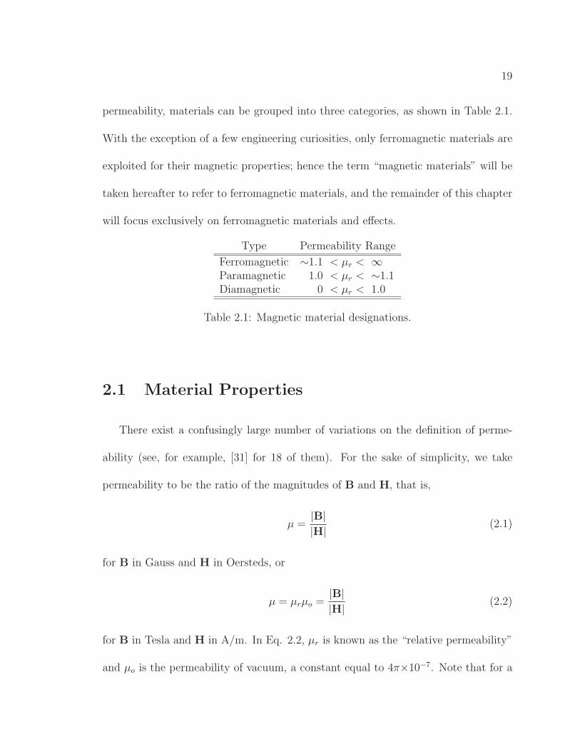
permeability, materials can be grouped into three categories, as shown in Table 2.1.

With the exception of a few engineering curiosities, only ferromagnetic materials are

exploited for their magnetic properties; hence the term “magnetic materials” will be

taken hereafter to refer to ferromagnetic materials, and the remainder of this chapter

will focus exclusively on ferromagnetic materials and effects.

Type Permeability Range

Ferromagnetic ∼1.1 < µr < ∞Paramagnetic 1.0 < µr < ∼1.1Diamagnetic 0 < µr < 1.0

Table 2.1: Magnetic material designations.

2.1 Material Properties

There exist a confusingly large number of variations on the definition of perme-

ability (see, for example, [31] for 18 of them). For the sake of simplicity, we take

permeability to be the ratio of the magnitudes of B and H, that is,

µ =|B||H| (2.1)

for B in Gauss and H in Oersteds, or

µ = µrµo =|B||H| (2.2)

for B in Tesla and H in A/m. In Eq. 2.2, µr is known as the “relative permeability”

and µo is the permeability of vacuum, a constant equal to 4π×10−7. Note that for a

20

given material, µ in Eq. 2.1 has the same value as µr in Eq. 2.2. Hereafter, only the

SI units of Tesla and A/m will be used. Note that for ferromagnetic materials, µr

depends strongly on the particular operating point; it is always prudent to determine

how a given permeability was calculated.

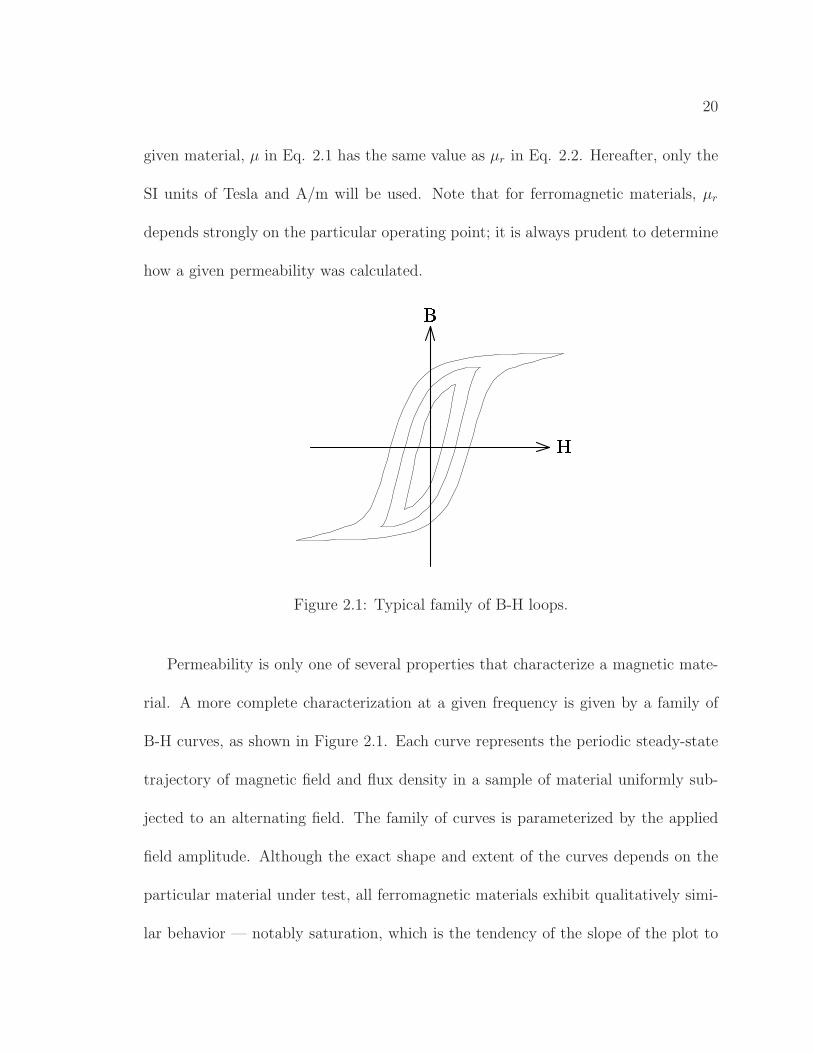
Figure 2.1: Typical family of B-H loops.

Permeability is only one of several properties that characterize a magnetic mate-

rial. A more complete characterization at a given frequency is given by a family of

B-H curves, as shown in Figure 2.1. Each curve represents the periodic steady-state

trajectory of magnetic field and flux density in a sample of material uniformly sub-

jected to an alternating field. The family of curves is parameterized by the applied

field amplitude. Although the exact shape and extent of the curves depends on the

particular material under test, all ferromagnetic materials exhibit qualitatively simi-

lar behavior — notably saturation, which is the tendency of the slope of the plot to

21

approach µo (i.e. µr=1) at high fields, and hysteresis, which is the multivalued nature

of the flux density for a given field.

The characteristic saturation and hysteresis of the ferromagnetic B-H loop are

the result of the material structure, in which atomic moments tend to self-align into

magnetic domains of relatively large extent (>0.1 µm [32]) in the absence of external

fields. The atomic moments within a domain are aligned, giving the domain a net

magnetization; however, the orientation of the magnetization from domain to domain

is random, resulting on average in a zero net magnetization for a given sample of

material. As the externally applied field is increased, initially domain boundaries

shift so as to increase the volume of the domains whose magnetization is parallel with

the applied field. This results in an increase in flux density. At higher levels of applied

field, domain magnetizations rotate to align with the field, increasing the flux density

further. However, at extremely high fields the great majority of domains are aligned,

and further increases in field fail to increase the flux beyond the increase expected

from vacuum. Thus the material saturates. The shifting of domain boundaries and

rotation of the domain magnetizations requires non-reversible work to be done by the

applied field. Hence the B-H loop must have a nonzero area equal to the net energy

required to traverse it; this is the origin of the hysteresis effect.

22

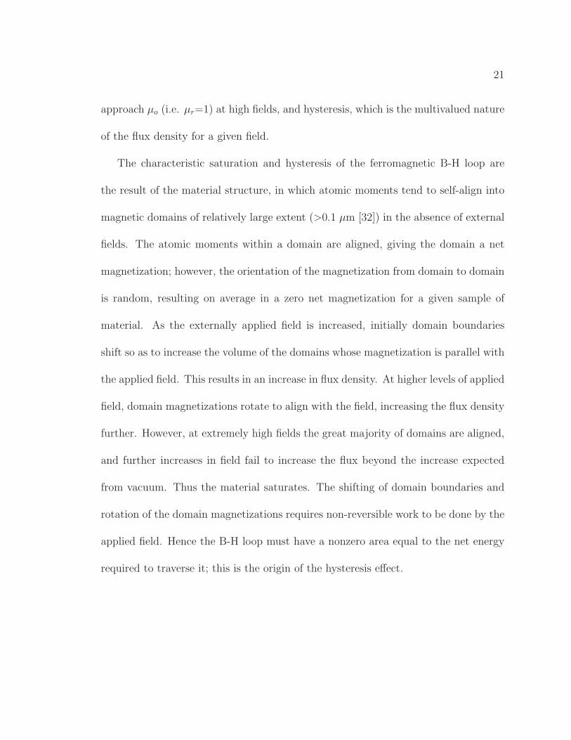
Figure 2.2: Typical B-H characteristic for soft magnetic material.

2.1.1 Soft Magnetic Materials

Soft magnetic materials are ferromagnetic materials with a narrow hysteresis char-

acteristic of the B-H loop, as shown in Fig. 2.2. The figure illustrates two critical

parameters for designing soft magnetic structures — the permeability and saturation

flux density or saturation induction. Given Equations 2.1 and 2.2, the permeability

appears as the slope of the plot. Saturation flux density (BSAT) is the value of flux

density at which the slope of the plot reaches µo, indicating that further field increases

will result in only the incremental flux increase expected from vacuum.

The analysis of magnetic structures is covered in Chapter 4; however brief remarks

on the implications of these quantities are offered here. Permeability determines the

ease with which magnetic flux can be induced to flow in a material. Because most

useful magnetic actuator designs incorporate an air gap with very low permeability,

23

permeability of a soft magnetic material is often of only secondary importance. Satu-

ration flux density, on the other hand, places a fundamental limit on the performance

of an electromechanical actuator (see Sec. 3.3.1). A low saturation value limits the

amount of stored energy, and hence limits the force or torque of an actuator. Typical

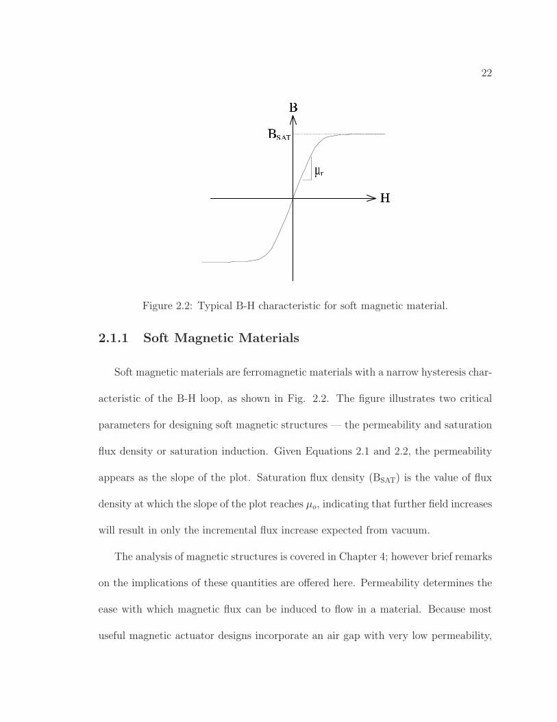
values for relative permeability and saturation flux density are given in Table 2.2.

Material µr BSAT (Tesla)

Fe 5000 2.158Co 245 1.787-1.875Ni 4800 0.608Ni80Fe20 840-7000 1.04Ni45Fe55 3500 1.62.75% Si Steel 5800 2.04

Table 2.2: Properties of selected soft magnetic materials [33].

2.1.2 Hard Magnetic Materials

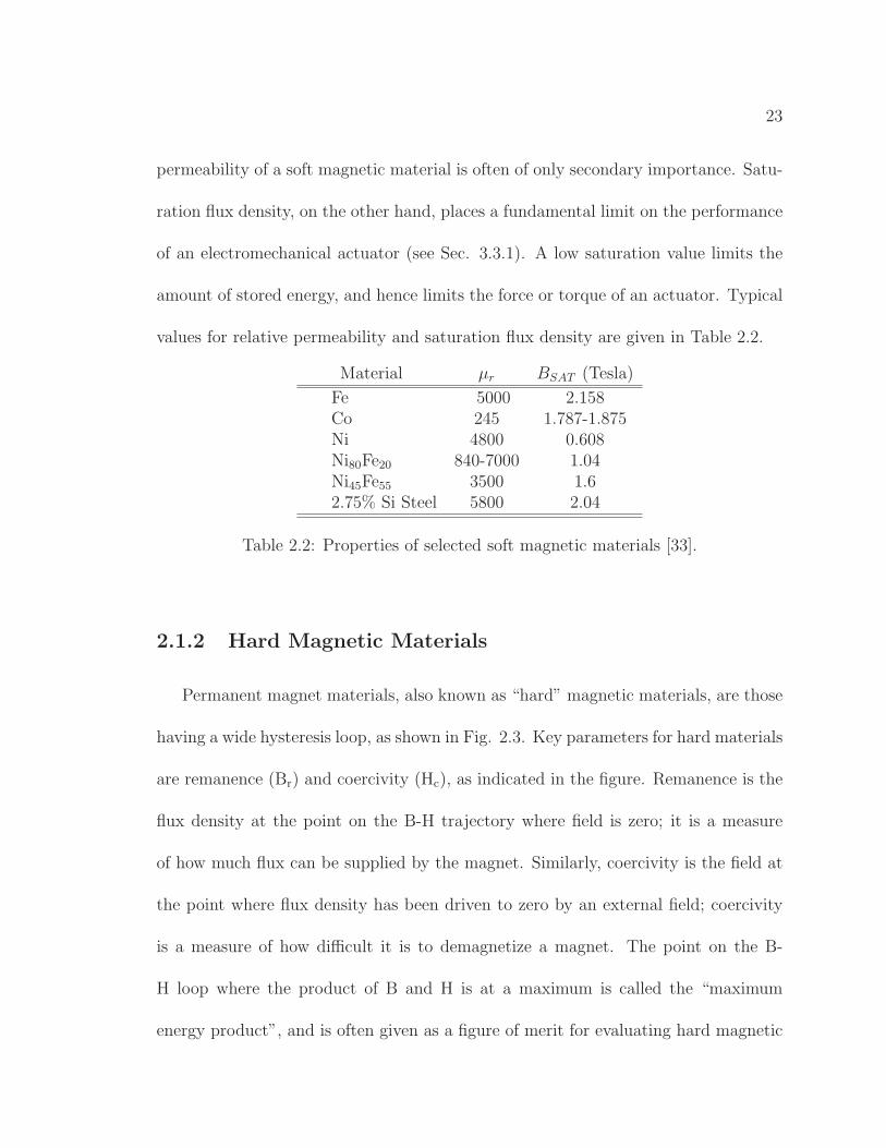
Permanent magnet materials, also known as “hard” magnetic materials, are those

having a wide hysteresis loop, as shown in Fig. 2.3. Key parameters for hard materials

are remanence (Br) and coercivity (Hc), as indicated in the figure. Remanence is the

flux density at the point on the B-H trajectory where field is zero; it is a measure

of how much flux can be supplied by the magnet. Similarly, coercivity is the field at

the point where flux density has been driven to zero by an external field; coercivity

is a measure of how difficult it is to demagnetize a magnet. The point on the B-

H loop where the product of B and H is at a maximum is called the “maximum

energy product”, and is often given as a figure of merit for evaluating hard magnetic

24

Figure 2.3: Typical B-H characteristic for hard magnetic material.

materials. Optimal designs use the magnet at or near its point of maximum energy

product.

Permanent magnets are useful because of the extremely large fields they can de-

velop in a small volume. For example, for a simple C-core with cross sectional di-

mensions of 1 cm by 1 cm and a 1 mm air gap, a magnet with Br = 0.7 and volume

of 1×10−6 m3 (i.e. a cube with 1 cm sides) can provide a uniform flux density of

0.636 Tesla in the gap. A copper winding that provides the same flux density in

the gap, operating with a current density of 10×106 A/m2 would have a volume of

approximately 2.03×10−6 m3 — a factor of two increase. Note also that unlike a

current-carrying conductor, the magnet does not dissipate power to provide field in

25

the gap. (Methods for calculation of fields due to permanent magnets are covered in

Chapter 4).

The magnetization of a permanent magnet is generally not intentionally changed

once it is assembled into an actuator. This can be a drawback, as in applications

where control over magnetic field is desired, or a useful feature, as in applications

where field is desired even when external power sources are unavailable.

There are numerous types of permanent magnet material; a detailed survey is be-

yond the scope of this work. The most commonly commonly used materials, however,

are alnico, ferrite, and the rare earth materials samarium cobalt and neodymium iron

boron.

Alnico is perhaps the oldest permanent magnet material still in widespread use, hav-

ing been discovered by Japanese researchers in 1931. It is capable of operating

at elevated temperatures, up to 520 C [34]. Alnico has high remanence, but

low coercivity, making it easy to demagnetize. Further, alnico’s demagnetiza-

tion curve is highly nonlinear, with the result that a freshly magnetized alnico

magnet can become partially demagnetized upon removal from the magnetizing

fixture. Thus to achieve the best performance, it may be necessary to magnetize

alnico magnets in place, only after a magnetic structure has been assembled. A

final consideration is the material’s brittleness. This makes machining difficult,

and increases the cost of parts that require close tolerances.

26

Ferrite magnets, also known as ceramic magnets, are alloys of Barium (Ba) or Stron-

tium (Sr) with ferrite (Fe2O3). The materials have a linear demagnetization

characteristic, and hence are easier to work with than alnico. This, and ferrites’

low cost make them the most common magnets for general purpose applications.

Samarium cobalt (SmCo), along with Neodymium, falls under the heading of “rare

earth” permanent magnet materials. Samarium cobalt is a high performance

material, having high remanence and coercivity, and a linear demagnetization

curve. It is expensive, however, owing to the high cost of the component Sm

and Co.

Neodymium iron boron (NdFeB) magnets are a relatively recent development,

becoming available in the early 1980s. Because Nd is more readily available

than Sm, they are less expensive than SmCo. Neodymium magnets currently

have the best magnetic properties at room temperature. However, the material

is sensitive to high temperatures, with a maximum operating temperature of

250 C. Neodymium magnets can also corrode if proper precautions are not

taken.

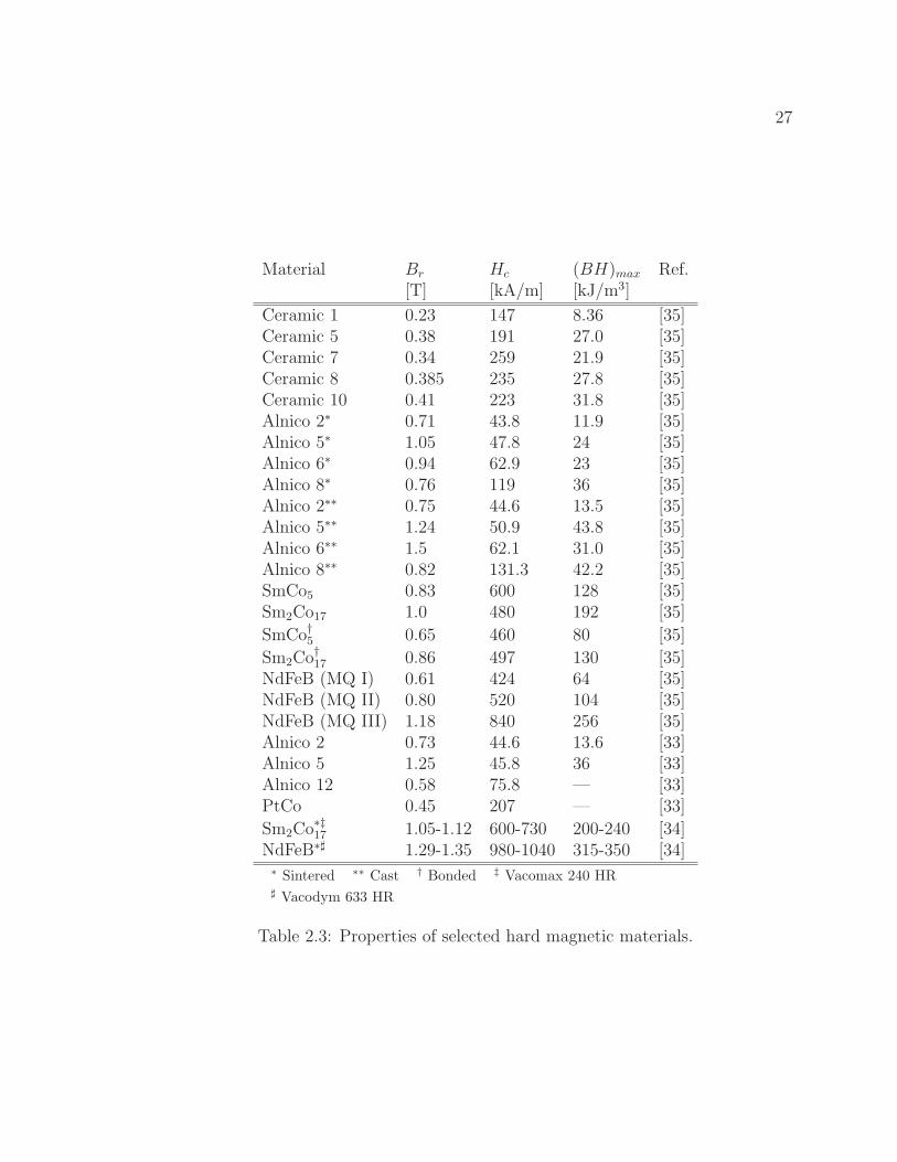
Table 2.3 summarizes the properties of these materials.

27

Material Br Hc (BH)max Ref.[T] [kA/m] [kJ/m3]

Ceramic 1 0.23 147 8.36 [35]Ceramic 5 0.38 191 27.0 [35]Ceramic 7 0.34 259 21.9 [35]Ceramic 8 0.385 235 27.8 [35]Ceramic 10 0.41 223 31.8 [35]Alnico 2∗ 0.71 43.8 11.9 [35]Alnico 5∗ 1.05 47.8 24 [35]Alnico 6∗ 0.94 62.9 23 [35]Alnico 8∗ 0.76 119 36 [35]Alnico 2∗∗ 0.75 44.6 13.5 [35]Alnico 5∗∗ 1.24 50.9 43.8 [35]Alnico 6∗∗ 1.5 62.1 31.0 [35]Alnico 8∗∗ 0.82 131.3 42.2 [35]SmCo5 0.83 600 128 [35]Sm2Co17 1.0 480 192 [35]

SmCo†5 0.65 460 80 [35]

Sm2Co†17 0.86 497 130 [35]NdFeB (MQ I) 0.61 424 64 [35]NdFeB (MQ II) 0.80 520 104 [35]NdFeB (MQ III) 1.18 840 256 [35]Alnico 2 0.73 44.6 13.6 [33]Alnico 5 1.25 45.8 36 [33]Alnico 12 0.58 75.8 — [33]PtCo 0.45 207 — [33]

Sm2Co∗‡17 1.05-1.12 600-730 200-240 [34]NdFeB∗♯ 1.29-1.35 980-1040 315-350 [34]∗ Sintered ∗∗ Cast † Bonded ‡ Vacomax 240 HR♯ Vacodym 633 HR

Table 2.3: Properties of selected hard magnetic materials.

28

2.2 Temperature Effects

All ferromagnetic materials experience a drop in saturation flux density as temper-

ature increases. This drop is gradual at first, becomes steep at higher temperatures,

and levels off again as the value approaches zero. The Curie point, or Curie temper-

ature, is the extrapolation of the steep part of the curve to zero saturation. Above

this temperature, saturation is effectively, if not identically, zero. Physically, when

temperature is below the Curie point, fields resulting from atomic moments cause an

ordered domain structure; above the Curie point thermal effects dominate, pushing

the structure towards disorder [32]. Table 2.4 gives Curie points for some common

soft magnetic materials.

Material Curie Point (C) Ref.

Fe 770 [33]Co 1130 [33]Ni 358 [33]Ni80Fe20 560† [33]Ni50Fe50 530† [33]2.75% Si Steel 760† [33]Alnico 5∗ 900 [35]Ceramic 10 450 [35]Sm2Co17 750 [35]NdFeB (MQIII) 312 [35]∗ Sintered † Approximate

Table 2.4: Curie point of selected magnetic materials.

29

2.3 Frequency Effects

The design of magnetic structures is treated extensively in Chapter 4. However,

the skin depth, a measure of the depth of penetration of an AC magnetic field, and

core loss, energy dissipated by AC fields, both depend on material properties as well as

operating point. Hence they appropriately fit into a discussion of material properties,

but must be considered in the context of design.

2.3.1 Skin Effect at High Frequency

The skin effect, with reference to magnetic fields, describes the tendency of alter-

nating magnetic fields in soft magnetic materials to achieve maximum value at the

surface of an object, while decreasing in amplitude towards the center. The layer of

high flux density forms a “skin” on the object. The skin effect is the result of circu-

lating eddy currents, which tend to cancel some of the field. In practice, if the skin

depth of a material at the desired operating frequency is smaller than the thickness

of the structure, quasi-static calculations will overestimate the amount of flux carried

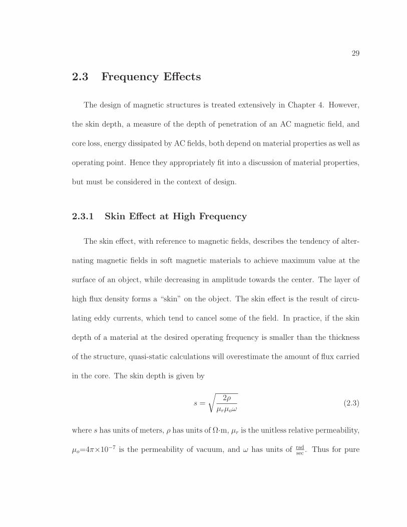
in the core. The skin depth is given by

s =

√

2ρ

µrµoω(2.3)

where s has units of meters, ρ has units of Ω·m, µr is the unitless relative permeability,

µo=4π×10−7 is the permeability of vacuum, and ω has units of radsec

. Thus for pure

30

iron (µr=5000, ρ=97×10−9 Ω·m) at 500 Hz (ω=3142 radsec

), Eq. 2.3 gives

s =

√

2 · 97×10−9

5000 · 4π×10−7 · 3142∼= 100×10−6 m (2.4)

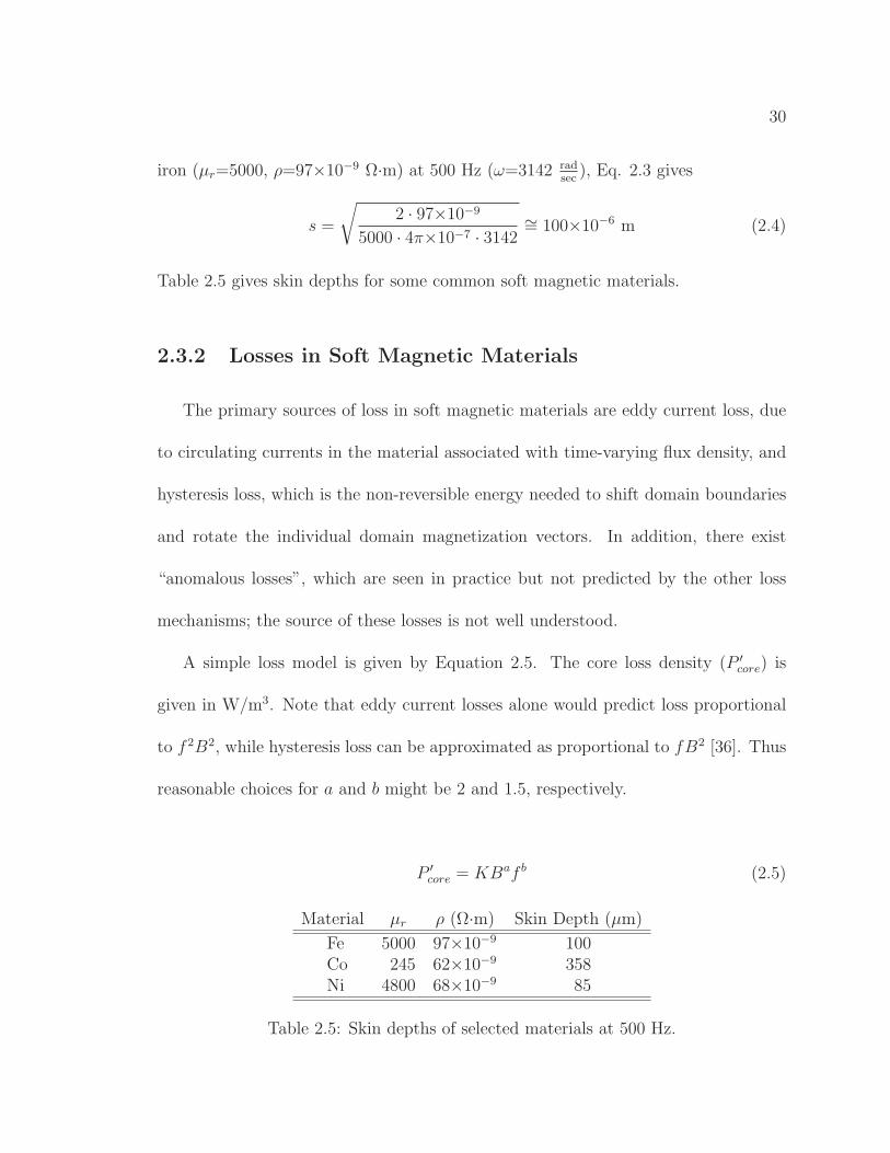
Table 2.5 gives skin depths for some common soft magnetic materials.

2.3.2 Losses in Soft Magnetic Materials

The primary sources of loss in soft magnetic materials are eddy current loss, due

to circulating currents in the material associated with time-varying flux density, and

hysteresis loss, which is the non-reversible energy needed to shift domain boundaries

and rotate the individual domain magnetization vectors. In addition, there exist

“anomalous losses”, which are seen in practice but not predicted by the other loss

mechanisms; the source of these losses is not well understood.

A simple loss model is given by Equation 2.5. The core loss density (P ′core) is

given in W/m3. Note that eddy current losses alone would predict loss proportional

to f 2B2, while hysteresis loss can be approximated as proportional to fB2 [36]. Thus

reasonable choices for a and b might be 2 and 1.5, respectively.

P ′core = KBaf b (2.5)

Material µr ρ (Ω·m) Skin Depth (µm)

Fe 5000 97×10−9 100Co 245 62×10−9 358Ni 4800 68×10−9 85

Table 2.5: Skin depths of selected materials at 500 Hz.

31

Several measures can be taken to mitigate core loss. From a design standpoint,

lower flux densities and lower frequencies should be used when feasible. Materials

having higher resistivities, such as ferrites, can reduce eddy current losses, while

those with narrow B-H loops can reduce hysteresis loss. Finally, composite materials

can be fashioned such that electrical insulation introduced into the magnetic structure

limits eddy current losses. Such low-loss materials include silicon-iron alloy (silicon

steel) formed into thin laminated layers, powdered iron (also known as SMC or soft

magnetic composite).

P ′core =

Kfa

B3 + bB2.3 + c

B1.65

+ df 2B2 (2.6)

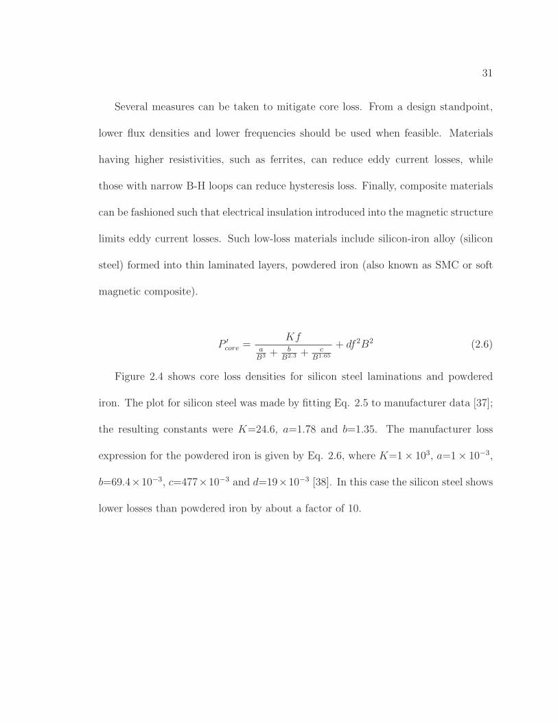
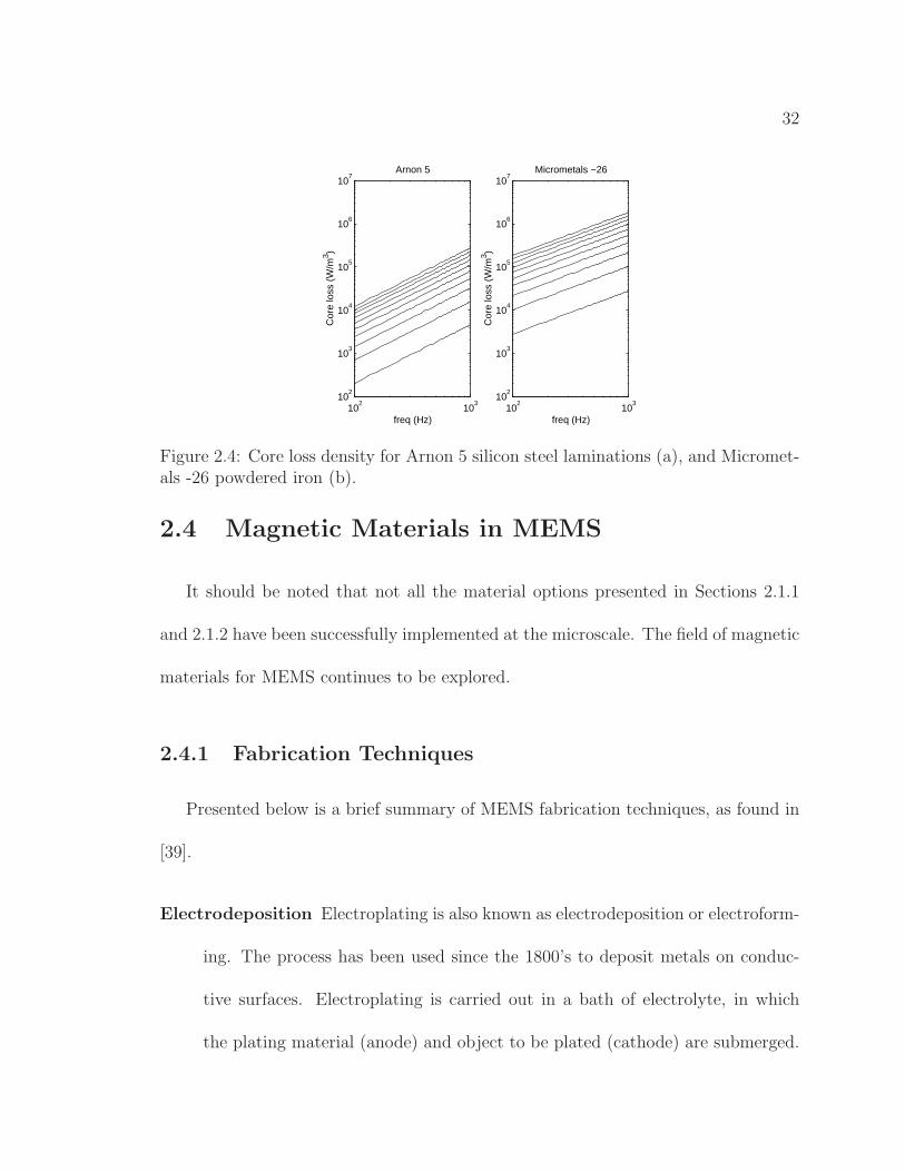
Figure 2.4 shows core loss densities for silicon steel laminations and powdered

iron. The plot for silicon steel was made by fitting Eq. 2.5 to manufacturer data [37];

the resulting constants were K=24.6, a=1.78 and b=1.35. The manufacturer loss

expression for the powdered iron is given by Eq. 2.6, where K=1× 103, a=1× 10−3,

b=69.4×10−3, c=477×10−3 and d=19×10−3 [38]. In this case the silicon steel shows

lower losses than powdered iron by about a factor of 10.

32

102

103

102

103

104

105

106

107

Arnon 5

freq (Hz)

Cor

e lo

ss (

W/m

3 )

102

103

102

103

104

105

106

107

Micrometals −26

freq (Hz)

Cor

e lo

ss (

W/m

3 )

Figure 2.4: Core loss density for Arnon 5 silicon steel laminations (a), and Micromet-als -26 powdered iron (b).

2.4 Magnetic Materials in MEMS

It should be noted that not all the material options presented in Sections 2.1.1

and 2.1.2 have been successfully implemented at the microscale. The field of magnetic

materials for MEMS continues to be explored.

2.4.1 Fabrication Techniques

Presented below is a brief summary of MEMS fabrication techniques, as found in

[39].

Electrodeposition Electroplating is also known as electrodeposition or electroform-

ing. The process has been used since the 1800’s to deposit metals on conduc-

tive surfaces. Electroplating is carried out in a bath of electrolyte, in which

the plating material (anode) and object to be plated (cathode) are submerged.

33

An electrical current carries ions from the anode to the cathode, creating a

conformal coating. If specific shapes are desired for the deposited structures,

electroplating can be performed in conjunction with a mold.

Sputtering Sputtering is often used for the deposition of metal films, although it is

also suitable for amorphous silicon, glass and piezoelectric materials. Although

there are several variations, the essential mechanism is the firing of ions at a

target made from the desired deposition material. Particles displaced from the

target are guided towards the wafer by electric and/or magnetic fields. Sputter-

ing gives good conformality (uniform feature coverage), and can be performed

at relatively low temperatures. A drawback is high stress in deposited films,

and difficulty of precisely controlling film stress.

Evaporation Evaporation is another thin-film deposition technique, in which a tar-

get is heated with an electrical current or electron beam. Vaporized target

material then condenses on the wafer. This is a directional process, which can

result in “shadowing” effects if the wafer is not rotated.

LIGA LIGA is a multistep process that combines lithography, plating and molding

(hence the German acronym Lithographie, Galvanoformung und Abformung).

Relatively thick, high aspect ratio metal structures can be formed with this

process. X-ray lithography is used, which makes LIGA expensive and somewhat

inconvenient.

34

Other Techniques Various other techniques such as screen printing and molding

can also be employed.

2.4.2 Soft Magnetic Materials for MEMS

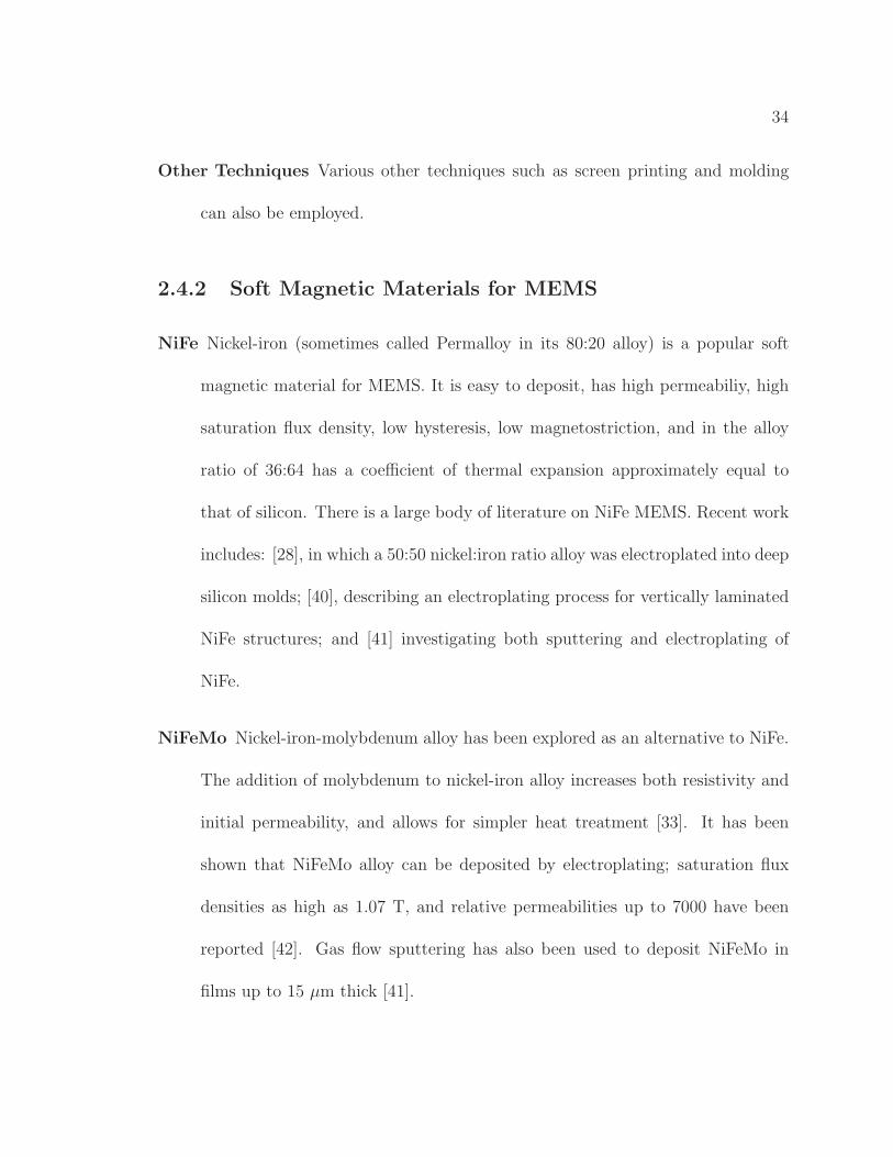
NiFe Nickel-iron (sometimes called Permalloy in its 80:20 alloy) is a popular soft

magnetic material for MEMS. It is easy to deposit, has high permeabiliy, high

saturation flux density, low hysteresis, low magnetostriction, and in the alloy

ratio of 36:64 has a coefficient of thermal expansion approximately equal to

that of silicon. There is a large body of literature on NiFe MEMS. Recent work

includes: [28], in which a 50:50 nickel:iron ratio alloy was electroplated into deep

silicon molds; [40], describing an electroplating process for vertically laminated

NiFe structures; and [41] investigating both sputtering and electroplating of

NiFe.

NiFeMo Nickel-iron-molybdenum alloy has been explored as an alternative to NiFe.

The addition of molybdenum to nickel-iron alloy increases both resistivity and

initial permeability, and allows for simpler heat treatment [33]. It has been

shown that NiFeMo alloy can be deposited by electroplating; saturation flux

densities as high as 1.07 T, and relative permeabilities up to 7000 have been

reported [42]. Gas flow sputtering has also been used to deposit NiFeMo in

films up to 15 µm thick [41].

35

CoFe- and CoNi- Alloys A large body of literature exists detailing magnetic ma-

terials that find application in the magnetic recording and data storage industry.

Although few MEMS applications have been reported, these alloys are nonethe-

less potential candidates for sensors and actuators: CoFeB; CoFeCr; CoFeP;

CoFeCu; CoNiFe; CoNiFeS; CoFeNiCr; CoFeSnP; and CoNiFeB [43].

2.4.3 Hard Magnetic Materials for MEMS

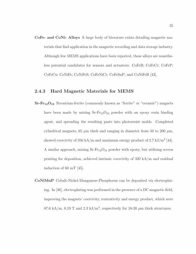
Sr-Fe12O19 Strontium-ferrite (commonly known as “ferrite” or “ceramic”) magnets

have been made by mixing Sr-Fe12O19 powder with an epoxy resin binding

agent, and spreading the resulting paste into photoresist molds. Completed

cylindrical magnets, 65 µm thick and ranging in diameter from 50 to 200 µm,

showed coercivity of 356 kA/m and maximum energy product of 2.7 kJ/m3 [44].

A similar approach, mixing Sr-Fe12O19 powder with epoxy, but utilizing screen

printing for deposition, achieved intrinsic coercivity of 320 kA/m and residual

induction of 60 mT [45].

CoNiMnP Cobalt-Nickel-Manganese-Phosphorus can be deposited via electroplat-

ing. In [46], electroplating was performed in the presence of a DC magnetic field,

improving the magnets’ coercivity, rententivity and energy product, which were

87.6 kA/m, 0.19 T and 2.3 kJ/m3, respectively for 18-20 µm thick structures.

36

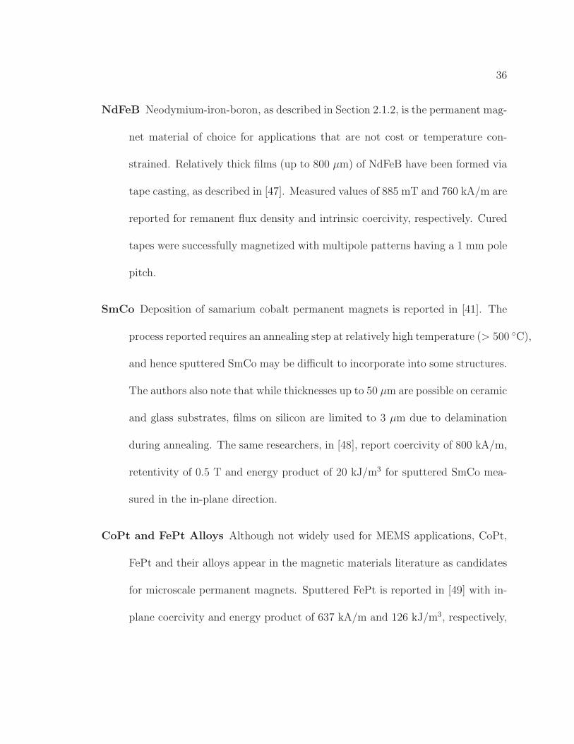
NdFeB Neodymium-iron-boron, as described in Section 2.1.2, is the permanent mag-

net material of choice for applications that are not cost or temperature con-

strained. Relatively thick films (up to 800 µm) of NdFeB have been formed via

tape casting, as described in [47]. Measured values of 885 mT and 760 kA/m are

reported for remanent flux density and intrinsic coercivity, respectively. Cured

tapes were successfully magnetized with multipole patterns having a 1 mm pole

pitch.

SmCo Deposition of samarium cobalt permanent magnets is reported in [41]. The

process reported requires an annealing step at relatively high temperature (> 500 C),

and hence sputtered SmCo may be difficult to incorporate into some structures.

The authors also note that while thicknesses up to 50 µm are possible on ceramic

and glass substrates, films on silicon are limited to 3 µm due to delamination

during annealing. The same researchers, in [48], report coercivity of 800 kA/m,

retentivity of 0.5 T and energy product of 20 kJ/m3 for sputtered SmCo mea-

sured in the in-plane direction.

CoPt and FePt Alloys Although not widely used for MEMS applications, CoPt,

FePt and their alloys appear in the magnetic materials literature as candidates

for microscale permanent magnets. Sputtered FePt is reported in [49] with in-

plane coercivity and energy product of 637 kA/m and 126 kJ/m3, respectively,

37

while electroplated CoPtW(P) and CoPtZn(P) having coercivity as high as 300

kA/m are reported in [50].

38

Chapter 3

Electric Machine Technology

This chapter attempts to provide an overview of electric machine technology. By

necessity the treatment is superficial and incomplete. It is worthwhile however, con-

sidering the nature of the reported research. The goal of the chapter is to document

technologies that are appropriate for portable electric power generation, and provide

information on the state of the art. In addition to serving as a basis for evaluation of

the designs presented in Chapters 5 and 6, this chapter may also be useful as a refer-

ence for the reader interested in selecting small electric motors or generators. Many

of the concepts here are extremely basic for the reader familiar with electric machines.

However, the information is included to aid in defining terms used throughout this

work, and to make the work accessible to as wide an audience as possible. While

reference will be made to basic results concerning the analysis of electromechanical

devices, detailed analysis is left for Chapter 4.

39

The focus here is on machines that may be considered for portable applications.

DC machines are neglected due to their poor reliability. Further, only rotary ma-

chines and primarily electromagnetic actuation are considered; machines making use

of electric fields make an appearance only at the micro scale. The first section intro-

duces the various means by which torque can be developed from magnetic and electric

fields. The second section presents different rotary machine configurations that can

make use of these torque-producing effects. The third section gives a scaling analysis

along with design implications for small-scale machines. The last section gives rel-

evant data on existing macro-scale and micro-scale machines, including commercial

devices as well as state of the art research examples.

3.1 Electric Machine Types

3.1.1 Reluctance

Reluctance is the simplest electromagnetic mechanism for producing a torque.

Reluctance forces are those that attract soft magnetic materials to a magnetic field.

Typically, a reluctance machine consists of a soft magnetic stator with wound con-

ductors, and a soft magnetic rotor. The rotor must have either saliency (non-uniform

shape) or anisotropy (non-uniform permeability), while the stator may be uniform,

salient, or anisotropic. When a winding is energized, torque acts to minimize the

40

reluctance of the magnetic circuit formed by the rotor and stator. By energizing

multiple windings in sequence, the rotor can be made to turn.

Several types of machine depend on reluctance effects to develop torque: syn-

chronous reluctance machines (SRMs); switched reluctance, variable reluctance or

“stepper” motors. The advantages of the reluctance machine are its robust construc-

tion, low cost, precise positioning capability, and ability to hold a static position.

3.1.2 Electromagnetic Induction

Induction machines typically have a soft magnetic stator and rotor separated by

a uniform air gap, a wound stator, and windings or other conductive material (e.g.

copper bars) in the rotor. Because the stator and rotor are coupled magnetically, AC

currents in the stator will excite currents in the rotor, much like in a transformer. The

interaction of the magnetic fluxes resulting from rotor and stator currents produces

torque. However, should the rotor speed rise to become synchronous with the stator

electrical frequency, the frequency of the stator excitation relative to the rotor is

zero, no current is excited in the rotor, and the machine loses torque. Thus induction

machines are inherently asynchronous — the rotor does not move in lock-step with

the stator frequency.

Induction machines are the most commonly used in industrial settings and in home

appliances because of their simplicity of operation and low cost. Because they are

open loop stable with a wide range of attraction, no sensors or closed-loop controls

41

are needed to run the machine for simple line-connected applications like fans and

pumps. And because the machine can start up and run from AC line power, no

semiconductor elements are needed for these applications. Induction machines are

less common in small-scale and portable applications, where power density is critical.

3.1.3 Permanent Magnet

As the name implies, permanent magnet machines employ hard magnetic ma-

terials, usually in the rotor. The interaction of the stator windings with the field

produced by the magnets gives rise to torque. Permanent magnet machines typically

have higher specific torque, specific power and efficiency than other types of machines

because of the high field provided by the magnets. Recall the example given in Section

2.1.2; compared to a winding providing the same field, permanent magnet excitation

requires less volume and mass, and does not carry the penalty of resistive power loss.

Permanent magnet machines fall into two main categories: permanent magnet

synchronous machines (PMSM); and brushless DC (BLDC). PMSMs are excited by

sinusoidal voltages, and often operate without direct sensing of position. BLDC

machines are excited by square-wave voltages, and feature electronic commutation,

in which feedback from position sensors (often hall effect sensors) determines the

correct phase excitation to be supplied by the inverter. Note that BLDC machines

are not true DC machines, but only appear so to the end user because they are

42

packaged with sensors and drive electronics that perform the function of traditional

mechanical brushes.

Type Self exciting Holding torque Synchronous Torque

Reluctance No Yes Yes LowInduction No No No ModeratePermanent Magnet Yes Yes Yes High

Table 3.1: Comparison of electric machine technologies.

3.1.4 Electrostatic

Due to both practical and fundamental limitations, electrostatic machines are not

competitive at the macro-scale. However, at extremely small size scales the technology

begins to look more attactive, as explained in Sec. 3.3.1. Thus many MEMS devices

utilize electrostatic actuation. Such devices will not be discussed in this work; the

reader is directed to the copious literature on MEMS actuators.

3.2 Electric Machine Configurations

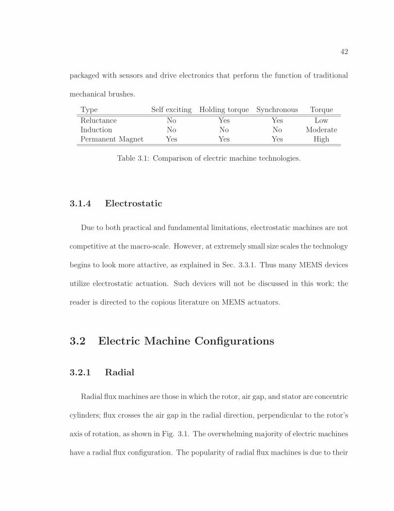
3.2.1 Radial

Radial flux machines are those in which the rotor, air gap, and stator are concentric

cylinders; flux crosses the air gap in the radial direction, perpendicular to the rotor’s

axis of rotation, as shown in Fig. 3.1. The overwhelming majority of electric machines

have a radial flux configuration. The popularity of radial flux machines is due to their

43

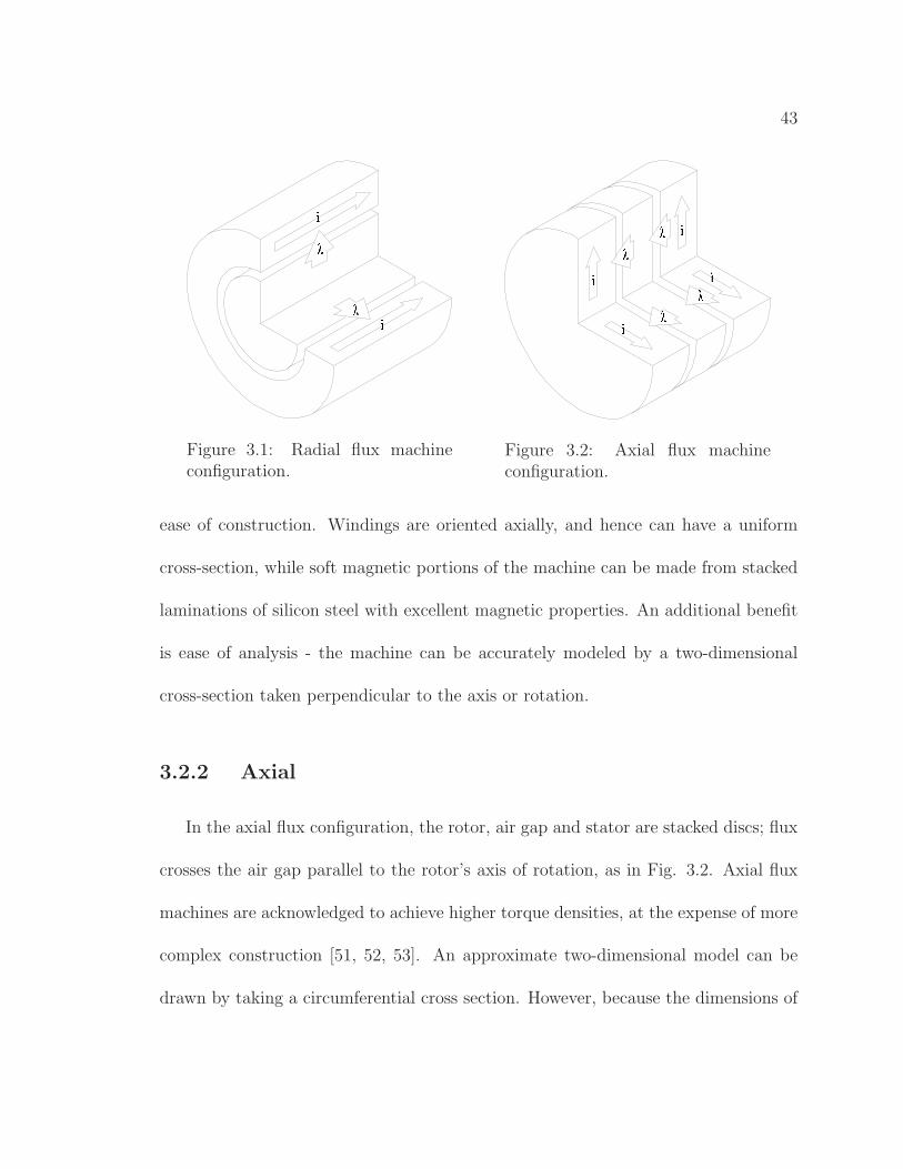
Figure 3.1: Radial flux machineconfiguration.

Figure 3.2: Axial flux machineconfiguration.

ease of construction. Windings are oriented axially, and hence can have a uniform

cross-section, while soft magnetic portions of the machine can be made from stacked

laminations of silicon steel with excellent magnetic properties. An additional benefit

is ease of analysis - the machine can be accurately modeled by a two-dimensional

cross-section taken perpendicular to the axis or rotation.

3.2.2 Axial

In the axial flux configuration, the rotor, air gap and stator are stacked discs; flux

crosses the air gap parallel to the rotor’s axis of rotation, as in Fig. 3.2. Axial flux

machines are acknowledged to achieve higher torque densities, at the expense of more

complex construction [51, 52, 53]. An approximate two-dimensional model can be

drawn by taking a circumferential cross section. However, because the dimensions of

44

the model depend on the particular radius chosen for the cross-section, the model is

not exact.

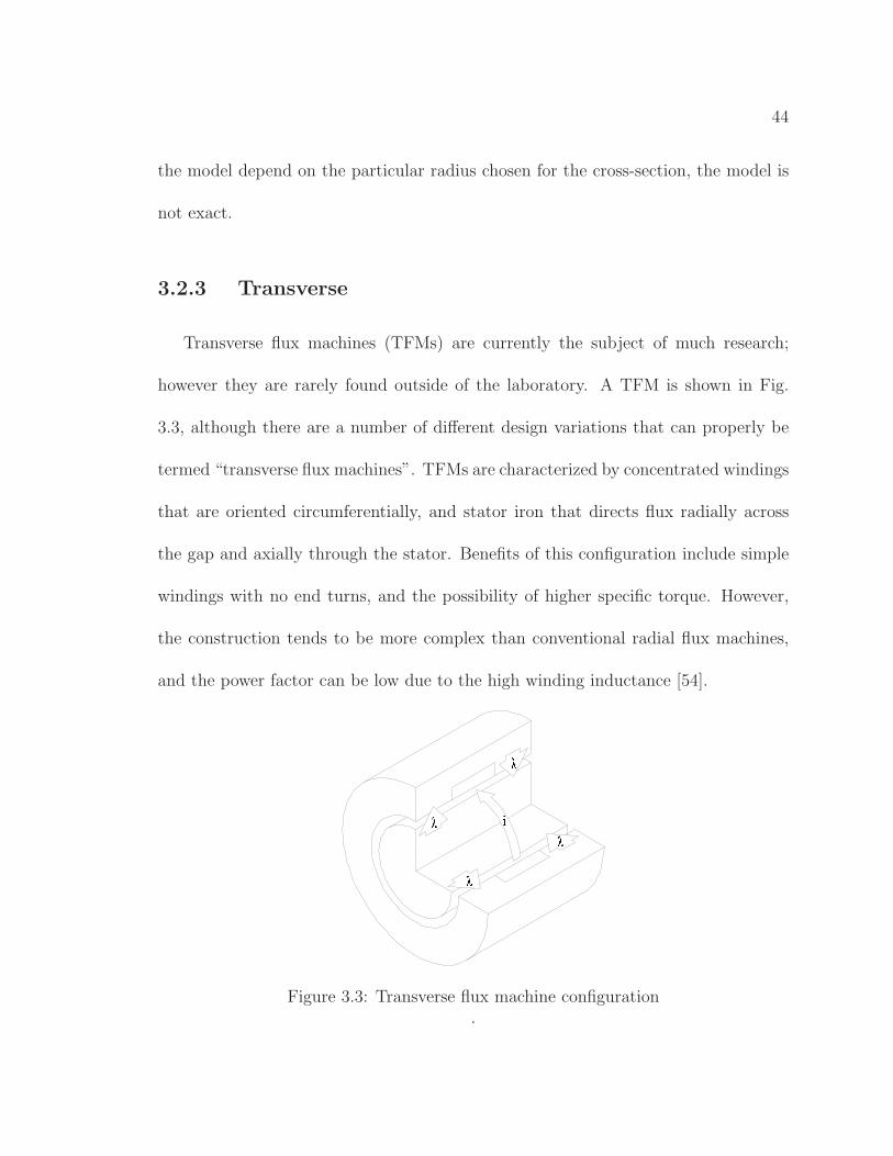
3.2.3 Transverse

Transverse flux machines (TFMs) are currently the subject of much research;

however they are rarely found outside of the laboratory. A TFM is shown in Fig.

3.3, although there are a number of different design variations that can properly be

termed “transverse flux machines”. TFMs are characterized by concentrated windings

that are oriented circumferentially, and stator iron that directs flux radially across

the gap and axially through the stator. Benefits of this configuration include simple

windings with no end turns, and the possibility of higher specific torque. However,

the construction tends to be more complex than conventional radial flux machines,

and the power factor can be low due to the high winding inductance [54].

Figure 3.3: Transverse flux machine configuration.

45

3.3 Scaling of Electromechanical Actuators

3.3.1 Fundamental Limits

There are fundamental limits to the amount of force or torque an electromagnetic

or electrostatic actuator can produce. As described in Chapter 4, force is developed

when the amount of stored energy in an electric or magnetic field changes with ac-

tuator displacement. Thus, in general, higher field intensities translate into larger

absolute changes in stored energy, and larger forces. The majority of energy storage

takes place in the gap (usually filled with air) that separates the stationary and mov-

ing portions of the actuator. So the highest field that can be established in an air

gap is a good figure of merit for the actuator.

For electrostatic actuators, the limitation on electric field is the electrostatic break-

down of the medium in the gap. When the field in the gap is too high (i.e. the voltage

across the gap is too high), a plasma arc will form, transferring all the charge from

high to low potential. With the field discharged, the actuator cannot produce force.

The field at which the arc forms depends on the medium as well as on pressure. The

empirical relation between electrostatic breakdown voltage and gap length is known

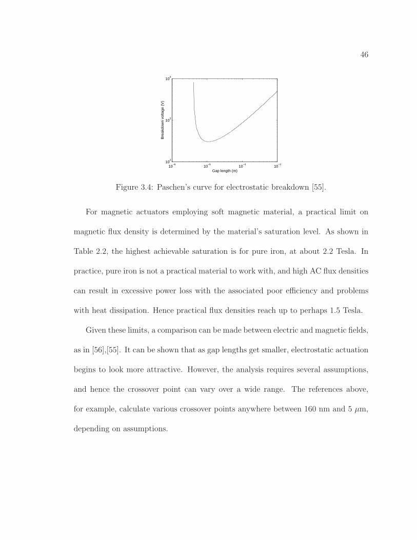
as the Paschen curve, shown in Fig. 3.4. It should be noted that to achieve the limits

of the Paschen curve, surfaces with high smoothness are required. Sharp points or

defects on the surface can cause localized field concentrations that cause breakdown

before the field limit is reached throughout the volume of the gap.

46

10−6

10−5

10−4

10−3

102

103

104

Gap length (m)

Bre

akdo

wn

volta

ge (

V)

Figure 3.4: Paschen’s curve for electrostatic breakdown [55].

For magnetic actuators employing soft magnetic material, a practical limit on

magnetic flux density is determined by the material’s saturation level. As shown in

Table 2.2, the highest achievable saturation is for pure iron, at about 2.2 Tesla. In

practice, pure iron is not a practical material to work with, and high AC flux densities

can result in excessive power loss with the associated poor efficiency and problems

with heat dissipation. Hence practical flux densities reach up to perhaps 1.5 Tesla.

Given these limits, a comparison can be made between electric and magnetic fields,

as in [56],[55]. It can be shown that as gap lengths get smaller, electrostatic actuation

begins to look more attractive. However, the analysis requires several assumptions,

and hence the crossover point can vary over a wide range. The references above,

for example, calculate various crossover points anywhere between 160 nm and 5 µm,

depending on assumptions.

47

3.3.2 Scaling of Electromagnetic Machines

The two critical specifications for an electric motor or generator in portable appli-

cations are specific power (i.e. power per mass), and efficiency. A machine with high

specific power contributes less mass to the application for a given power level, allow-

ing greater portability, greater functionality, or more energy storage (i.e. the saved

mass can be replaced by batteries, capacitors, or fuel). A high efficiency machine

increases run time for a given level of energy storage.

On the macro-scale, electric machines are often designed with specific power, ef-

ficiency, or a trade-off between the two in mind. Below, the effects of scaling down

a machine and their implications for design are examined. First some key quantities

are defined.

• Torque: The torque (τ) produced by a rotary electromagnetic actuator is pro-

portional to the product of the current (i) in the windings and the magnetic

flux (λ) linking those windings.

τ ∝ λi (3.1)

• Power: Both electrical power (Pe) and mechanical power (Pm) can be defined

as measures of energy transfer per time.

Pe = vi (3.2)

Pm = τω (3.3)

48

Here v indicates voltage and ω indicates angular speed of the shaft. Note that

voltage is given by the time derivative of flux. Thus for a two-pole machine

v = ddt

λ = ωλ. (3.4)

Substituting Eqs. 3.1 and 3.4 into Eq. 3.3, we see that for an ideal machine with

no losses, the average values of electrical and mechanical power are identical.

• Losses: There are three main sources of loss in electric machines: copper loss

(PCu); iron loss (PFe); and frictional loss (Pfr). Copper loss is simply power

dissipated by the resistance (R) of the windings

PCu = i2R. (3.5)

Iron loss, sometimes called core loss, is the result of time-varying magnetic

fields in the ferromagnetic materials that are used to constrain the flux in most

motors. Iron loss has a component due to eddy currents in the material, and

a component due to the hysteresis characteristic of the material’s BH loop.

Expressions for iron loss are usually obtained by fitting a curve to experimental

data, and are often quite complex (see Section 2.3.2 and Appendix B). For the

purposes of the scaling argument below however, core loss will be approximated

by

PFe ∝ ωB2 · volume. (3.6)

49

• Efficiency: The efficiency (η) of a machine is given by the fraction of input

power remaining after losses are subtracted. In motoring operation this implies

ηmot =Pmech

Pelec

(3.7)

while in generator operation

ηgen =Pelec

Pmech

. (3.8)

A scaling analysis proceeds from a thought experiment which begins with a macro-

size electric motor, and scales it down by a factor s (0 < s < 1) along each of the

three spatial dimensions, while holding the flux density (B), current density (J) and

speed (ω) constant.

Because λ = B · area and i = J · area, it can be seen from Eqs. 3.1 and 3.3 that

torque and power are both proportional to s4:

τ ∝ BJs4 (3.9)

P ∝ ωBJs4 (3.10)

The resistance of the motor windings is given by R = σ lengtharea

, and substituting into

Eq. 3.5 gives

PCu ∝ σJ2s3. (3.11)

From Eq. 5.3, iron loss is also proportional to volume:

PFe ∝ ωB2s3. (3.12)

50

Thus it can be seen that as s decreases, torque and power decrease rapidly. Further-

more, power density drops linearly

P

volume∝ ωBJs (3.13)

and efficiency drops as well

η ∝ 1 − σJ

ωBs− B

Js. (3.14)

3.3.3 Scaling Strategies

To maintain the levels of power density and efficiency associated with the macro-

scale as a machine is scaled down, scaling up of J and ω is warranted; B in most

designs is close to material saturation limits, and hence it is not reasonable to expect

that it can be scaled. Note that the thermal dissipation ability of windings is increased

as surface area becomes large relative to volume, and lower centrifugal forces and

higher mechanical resonances at small scale allow higher speeds.

A possible plan is to attempt to keep efficiency constant, by scaling J ∝ 1s

and

ω ∝ 1s2 , while holding B constant. Under this “constant efficiency” scheme, power

decreases only linearly, and specific power actually increases. Of course, as s becomes

very small, limitations arise from the viscous losses of the high-speed rotor as well as

higher order terms in the copper and iron loss.

51

3.4 Survey of Small Electric Machines

3.4.1 Macro-Scale Machines

A wide array of small machines exists for power levels in the tens to hundreds

of Watts. Rather than attempt to document this vast space, Tab. 3.2 is offered

to give a representative sample of high-performance permanent magnet machines.

These machines utilize high energy product magnets, and hence achieve impressive

specific power and power density. Further, the brushless design is low maintenance

and environmentally rugged. Any small machine proposed for portable power must

be measured against these machines.

3.4.2 Microfabricated Machines

Tiny rotational electric machines making use of microfabrication technology have

been described in the literature since at least the late 1980’s (see for example [59]). For

reasons explained in Section 3.3.1, the majority of these designs utilize electrostatic

forces for actuation. A review of such devices is beyond the scope of this work.

However, MEMS rotational actuators based on electromagnetic forces also appear

in the literature, and this section attempts to summarize a representative sample of

these.

Some of the earliest work is presented in [60], [61], [62]. The first paper describes

a two-pole, two-phase reluctance machine with a 400 µm diameter rotor that reached

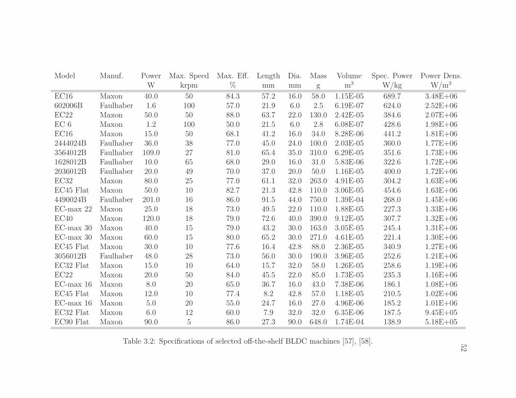
52

Model Manuf. Power Max. Speed Max. Eff. Length Dia. Mass Volume Spec. Power Power Dens.W krpm % mm mm g m3 W/kg W/m3

EC16 Maxon 40.0 50 84.3 57.2 16.0 58.0 1.15E-05 689.7 3.48E+06602006B Faulhaber 1.6 100 57.0 21.9 6.0 2.5 6.19E-07 624.0 2.52E+06EC22 Maxon 50.0 50 88.0 63.7 22.0 130.0 2.42E-05 384.6 2.07E+06EC 6 Maxon 1.2 100 50.0 21.5 6.0 2.8 6.08E-07 428.6 1.98E+06EC16 Maxon 15.0 50 68.1 41.2 16.0 34.0 8.28E-06 441.2 1.81E+062444024B Faulhaber 36.0 38 77.0 45.0 24.0 100.0 2.03E-05 360.0 1.77E+063564012B Faulhaber 109.0 27 81.0 65.4 35.0 310.0 6.29E-05 351.6 1.73E+061628012B Faulhaber 10.0 65 68.0 29.0 16.0 31.0 5.83E-06 322.6 1.72E+062036012B Faulhaber 20.0 49 70.0 37.0 20.0 50.0 1.16E-05 400.0 1.72E+06EC32 Maxon 80.0 25 77.0 61.1 32.0 263.0 4.91E-05 304.2 1.63E+06EC45 Flat Maxon 50.0 10 82.7 21.3 42.8 110.0 3.06E-05 454.6 1.63E+064490024B Faulhaber 201.0 16 86.0 91.5 44.0 750.0 1.39E-04 268.0 1.45E+06EC-max 22 Maxon 25.0 18 73.0 49.5 22.0 110.0 1.88E-05 227.3 1.33E+06EC40 Maxon 120.0 18 79.0 72.6 40.0 390.0 9.12E-05 307.7 1.32E+06EC-max 30 Maxon 40.0 15 79.0 43.2 30.0 163.0 3.05E-05 245.4 1.31E+06EC-max 30 Maxon 60.0 15 80.0 65.2 30.0 271.0 4.61E-05 221.4 1.30E+06EC45 Flat Maxon 30.0 10 77.6 16.4 42.8 88.0 2.36E-05 340.9 1.27E+063056012B Faulhaber 48.0 28 73.0 56.0 30.0 190.0 3.96E-05 252.6 1.21E+06EC32 Flat Maxon 15.0 10 64.0 15.7 32.0 58.0 1.26E-05 258.6 1.19E+06EC22 Maxon 20.0 50 84.0 45.5 22.0 85.0 1.73E-05 235.3 1.16E+06EC-max 16 Maxon 8.0 20 65.0 36.7 16.0 43.0 7.38E-06 186.1 1.08E+06EC45 Flat Maxon 12.0 10 77.4 8.2 42.8 57.0 1.18E-05 210.5 1.02E+06EC-max 16 Maxon 5.0 20 55.0 24.7 16.0 27.0 4.96E-06 185.2 1.01E+06EC32 Flat Maxon 6.0 12 60.0 7.9 32.0 32.0 6.35E-06 187.5 9.45E+05EC90 Flat Maxon 90.0 5 86.0 27.3 90.0 648.0 1.74E-04 138.9 5.18E+05

Table 3.2: Specifications of selected off-the-shelf BLDC machines [57], [58].

53

8 krpm with external magnetic excitation. The second paper represents a refinement

of the design, with a 3-phase variable reluctance machine having 6 stator poles and

4 rotor poles. The machine has integral windings for phase excitation as well as

photodiode rotor position sensors. Designs with 423 µm and 285 µm diameter rotors

achieved 12 krpm and 30 krpm, respectively. Neither of the first two papers give

estimates of machine torque or power. In the third paper, the design has evolved

to a 3-phase variable reluctance machine with a 50 tooth rotor which has diameter

of 1 mm. It is a hybrid MEMS-macro design, using hand-assembled wound coils for

excitation. The machine is coupled by a gear train to a MEMS dynamometer. A

maximum speed of 8 krpm, output torque of 0.3 µNm, and mechanical output power

of 20 µW are reported.

More recently, MEMS induction machines have been fabricated, as described in

[63], [64], [65]. Researchers at MIT have produced a microfabricated electromagnetic

induction motor with 8 mm diameter and 2 mm thickness. Experimentally demon-

strated torque of this machine is 1.2 uNm, although higher values are projected from

the data.

Researchers in Germany have produced a motor with 12.8 mm diameter and 1.4

mm thickness utilizing a combination of conventional techniques and microfabrication,

and have demonstrated a torque constant as high as 0.4 uNm/mA [66]. Another effort

there has microfabricated reluctance type linear stepper actuators with dimensions

of 8 mm by 1 mm [67], [68].

54

Chapter 4

Analysis of Electromechanical

Systems

This chapter is intended to provide the theoretical basis for the design and analy-

sis presented in Chapters 3, 5 and 6. The chapter begins by presenting Maxwell’s

equations for magnetic quasi-static fields, and explaining their significance. It is then

shown how, with the proper assumptions, the field equations can be rewritten to al-

low lumped-element analysis. The calculation of magnetic field quantities in simple

structures is presented as analogous to that of electrical quantities in electrical cir-

cuits. Provided with either lumped or distributed field calculations, a simple method

for the calculation of forces and torques can be derived from conservation of energy

assumptions. A brief overview is given of the finite-element method for magnetic field

55

solutions and its application to calculating forces and torques. Finally, the chapter

concludes with a detailed example of the various analyses.

The chapter does not address the analysis of electromechanical systems which

develop force from electrostatic fields. However, it can be shown that the analysis

given here does apply to such systems with a few minor changes. The chapter also

does not cover the Maxwell stress tensor, which can be used for force calculations;

the method is limited to distributed field solutions, and is not used for analysis in

any of the following chapters.

4.1 Maxwell’s Equations

In this section, the empirical results collectively known as Maxwell’s equations

are presented. The treatment is superficial, serving mainly as a basis for the devel-

opment of the lumped-element analysis presented in Section 4.2. For a more detailed

treatment of Maxwell’s equations as they relate to electromechanical interactions,

the interested reader is referred to [69] or the excellent appendices in [70]. Note also

that the quasi-static form of the equations is used below, in which some dynamic

effects (notably the displacement current in Ampere’s Law) are assumed to make

vanishingly small contributions over the frequency range of interest, and hence are

neglected. Throughout this chapter, H is magnetic field intensity, B is magnetic flux

density, J is current density, E is electric field intensity and n is an outward-pointing

normal vector, with boldface type indicating a vector quantity.

56

4.1.1 Quasi-static Magnetic Equations

Equation 4.1, also known as Ampere’s Law, relates magnetic field intensity and

electrical current density. Its practical implication is that a current-carrying wire acts

as a source of magnetic field. The contour C of the left-hand integral encloses the

surface S on the right, and hence the line integral of H traversing the contour is equal

to the area integral of current density passing through the surface.

∮

C

H · ~dℓ =

∫

S

J · n da (4.1)

If H can be constrained such that its value is constant and everywhere parallel to ~dℓ,

and the integral of the normal component of current density is defined as I, then 4.1

simplifies to

Hℓ = I (4.2)

where H and ℓ are scalar, and ℓ is the length of a path that encloses I.

Considering the right-hand side of Eq. 4.1, if S encloses a finite volume, Eq. 4.3

requires that the net current passing through S be zero. In other words, current flows

in a closed loop — there are no point sources or sinks of current. This can be thought

of as a general statement of the more familiar Kirchoff’s current law (KCL).

∮

S

J · n da = 0 (4.3)

Equation 4.4, also called Gauss’ Law, has the same form as Eq. 4.3, with magnetic

flux density substituted for current density. The implication is the same — magnetic

57

flux flows in closed loops, and Eq. 4.4 amounts to a version of KCL for magnetic flux.

∮

S

B · n da = 0 (4.4)

Finally, Eq. 4.5, known as Faraday’s Law, describes how changing magnetic flux

density induces an electric field. The time rate of change of the net flux through the

surface S is equal to the line integral of electric field along the contour C, where C

encloses S.∮

C

E · ~dℓ = − d

dt

∫

S

B · n da (4.5)

Equation 4.5 is often applied such that the C is coincident with a number of turns

(N) of conducting wire. The electric field is thus everywhere aligned with ~dℓ, and the

integral along the length of the wire gives the voltage across the two ends:

V =

∮

C

E · ~dℓ. (4.6)

Defining the flux through an open surface S as

Φ =

∮

S

B · nda, (4.7)

and flux linkage as

λ = NΦ, (4.8)

an expression for the voltage measured across the ends of the wire can be found by

substituting Eqs. 4.6-4.8 into 4.5:

V = − d

dtλ. (4.9)

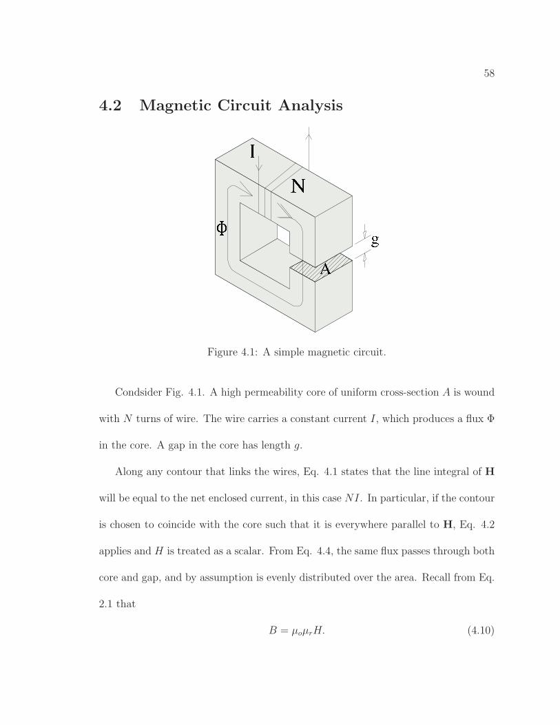
58

4.2 Magnetic Circuit Analysis

Figure 4.1: A simple magnetic circuit.

Condsider Fig. 4.1. A high permeability core of uniform cross-section A is wound

with N turns of wire. The wire carries a constant current I, which produces a flux Φ

in the core. A gap in the core has length g.

Along any contour that links the wires, Eq. 4.1 states that the line integral of H

will be equal to the net enclosed current, in this case NI. In particular, if the contour

is chosen to coincide with the core such that it is everywhere parallel to H, Eq. 4.2

applies and H is treated as a scalar. From Eq. 4.4, the same flux passes through both

core and gap, and by assumption is evenly distributed over the area. Recall from Eq.

2.1 that

B = µoµrH. (4.10)

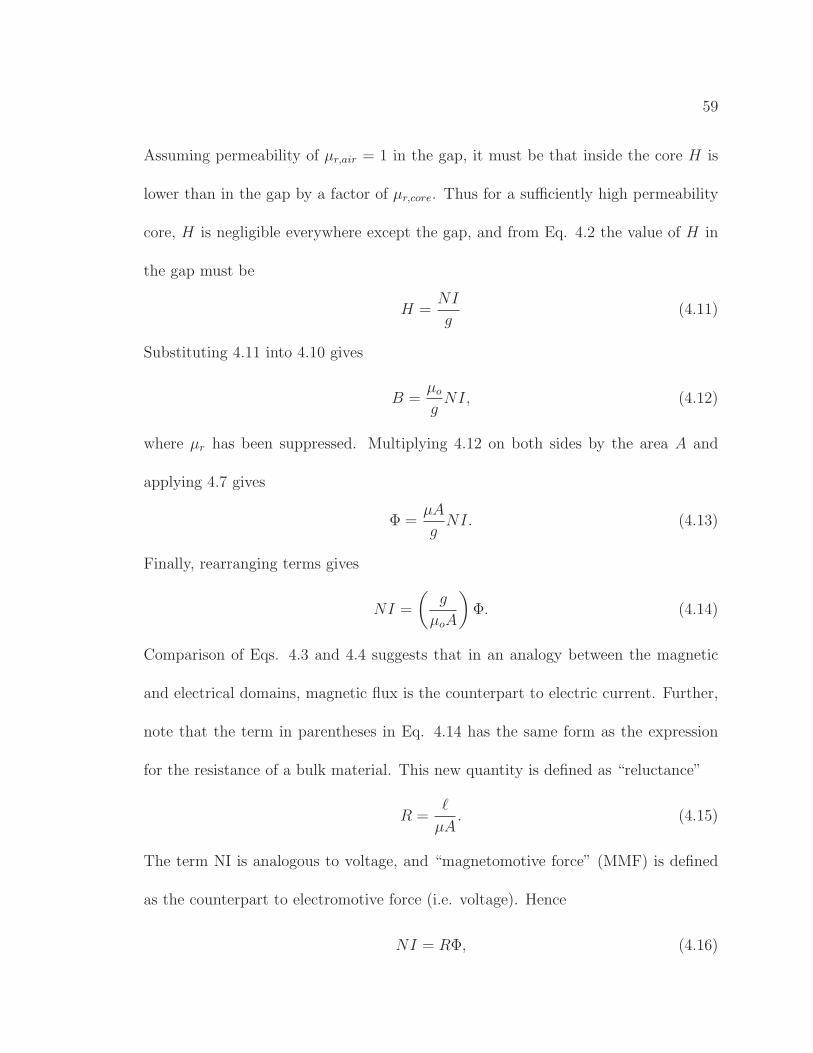
59

Assuming permeability of µr,air = 1 in the gap, it must be that inside the core H is

lower than in the gap by a factor of µr,core. Thus for a sufficiently high permeability

core, H is negligible everywhere except the gap, and from Eq. 4.2 the value of H in

the gap must be

H =NI

g(4.11)

Substituting 4.11 into 4.10 gives

B =µo

gNI, (4.12)

where µr has been suppressed. Multiplying 4.12 on both sides by the area A and

applying 4.7 gives

Φ =µA

gNI. (4.13)

Finally, rearranging terms gives

NI =

(

g

µoA

)

Φ. (4.14)

Comparison of Eqs. 4.3 and 4.4 suggests that in an analogy between the magnetic

and electrical domains, magnetic flux is the counterpart to electric current. Further,

note that the term in parentheses in Eq. 4.14 has the same form as the expression

for the resistance of a bulk material. This new quantity is defined as “reluctance”

R =ℓ

µA. (4.15)

The term NI is analogous to voltage, and “magnetomotive force” (MMF) is defined

as the counterpart to electromotive force (i.e. voltage). Hence

NI = RΦ, (4.16)

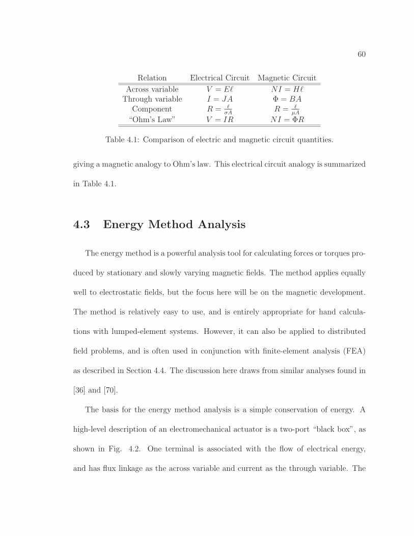
60

Relation Electrical Circuit Magnetic Circuit

Across variable V = Eℓ NI = HℓThrough variable I = JA Φ = BA

Component R = ℓσA

R = ℓµA

“Ohm’s Law” V = IR NI = ΦR

Table 4.1: Comparison of electric and magnetic circuit quantities.

giving a magnetic analogy to Ohm’s law. This electrical circuit analogy is summarized

in Table 4.1.

4.3 Energy Method Analysis

The energy method is a powerful analysis tool for calculating forces or torques pro-

duced by stationary and slowly varying magnetic fields. The method applies equally

well to electrostatic fields, but the focus here will be on the magnetic development.

The method is relatively easy to use, and is entirely appropriate for hand calcula-

tions with lumped-element systems. However, it can also be applied to distributed

field problems, and is often used in conjunction with finite-element analysis (FEA)

as described in Section 4.4. The discussion here draws from similar analyses found in

[36] and [70].

The basis for the energy method analysis is a simple conservation of energy. A

high-level description of an electromechanical actuator is a two-port “black box”, as

shown in Fig. 4.2. One terminal is associated with the flow of electrical energy,

and has flux linkage as the across variable and current as the through variable. The

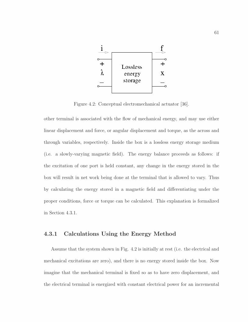
61

Figure 4.2: Conceptual electromechanical actuator [36].

other terminal is associated with the flow of mechanical energy, and may use either

linear displacement and force, or angular displacement and torque, as the across and

through variables, respectively. Inside the box is a lossless energy storage medium

(i.e. a slowly-varying magnetic field). The energy balance proceeds as follows: if

the excitation of one port is held constant, any change in the energy stored in the

box will result in net work being done at the terminal that is allowed to vary. Thus

by calculating the energy stored in a magnetic field and differentiating under the

proper conditions, force or torque can be calculated. This explanation is formalized

in Section 4.3.1.

4.3.1 Calculations Using the Energy Method

Assume that the system shown in Fig. 4.2 is initially at rest (i.e. the electrical and

mechanical excitations are zero), and there is no energy stored inside the box. Now

imagine that the mechanical terminal is fixed so as to have zero displacement, and

the electrical terminal is energized with constant electrical power for an incremental

62

time period dt. Since no mechanical work was done in this time, all of the energy

supplied to the terminal must have been stored inside the box. Thus an incremental

change in stored energy due to electrical excitation is given by

dWe = vidt, (4.17)

and substituting in Eq. 4.9 gives

dWe = (dλ

dt)idt = idλ. (4.18)

If λ is then held constant, and power fu (where f is force and u is velocity) is applied

to the mechanical terminal for incremental time dt, a similar incremental change in

stored energy will result. Noting that u = dxdt

, the incremental change in stored energy

due to mechanical excitation is

dWm = −fudt = −f(dx

dt)dt = −fdx. (4.19)

The total incremental change in stored energy is thus the sum of the electrical and

mechanical contributions,

dW = idλ − fdx. (4.20)

and total energy stored in the system for a given operating point (λo,xo) is given by

the integral

W =

∫ (λo,xo)

(0,0)

i(λ, x)dλ − f(λ, x)dx, (4.21)

where notation has changed slightly to indicate explicitly that i and f are functions

of λ and x.

63

Because the energy storage inside the black box is specified to be lossless, the

function W is uniquely defined for (λ, x) — i.e. W is a state, or potential, function.

Hence the value of W in Eq. 4.21 does not depend on the integration path between

the points (0,0) and (λo,xo). For mathematical simplicity, a convenient choice is a

path with two legs: zero flux linkage from x=0 to x=xo, implying zero force, and

constant displacement from λ=0 to λ=λo:

W (λo, xo) =

∫ xo

0

i(0, x)dλ − f(0, x)dx +

∫ λo

0

i(λ, xo)dλ − f(λ, xo)dx. (4.22)

Equation 4.22 can be interpreted as a zero force displacement (which contributes no

stored energy), followed by an increase in flux with displacement held constant (which

contributes energy from the electrical terminals only). Hence the first integral in Eq.

4.22 drops out entirely, and the second consists only of electrical quantities. Thus

W (λo, xo) =

∫ λo

0

i(λ, xo)dλ. (4.23)

Finally, note that an incremental change in energy can be written as

dW (λ, x) =∂W

∂λ

∣

∣

∣

∣

x=const

dλ +∂W

∂x

∣

∣

∣

∣

λ=const

dx, (4.24)

where it is critical that each partial derivative be taken with the other variable held

constant. Comparing Eqs. 4.20 and 4.24, it is clear that

i =∂W

∂λ

∣

∣

∣

∣

x=const

(4.25)

f = −∂W

∂x

∣

∣

∣

∣

λ=const

. (4.26)

Using Eq. 4.26, force can be determined from a change in stored energy.

64

4.3.2 Energy Versus Coenergy

The use of flux linkage as an independent variable is a significant drawback to the

energy method. Most engineers find it more natural to write down an expression for

flux linkage as a function of current rather than vice versa. More importantly, the

requirement that the partial derivative of Eq. 4.26 be taken with λ held constant

is particularly onerous; most finite-element analysis (FEA) problems are formulated

such that currents and material magnetization are held constant.

Fortunately, relief is available in the form of the “coenergy method”. Coenergy,

denoted Wc, can be thought of as a quantity that is equivalent, but not necessarily

equal, to energy. The strategy for using the coenergy to calculate force is identical to

that for energy, with the exception that current becomes the independent electrical

variable. This is accomplished via a Legendre transform, such that

Wc = λi − W. (4.27)

Figure 4.3 shows the graphical interpretation of the relationship between energy and

coenergy. On the plot of flux linkage versus current in the figure, energy is the area

W =∫

idλ as in Eq. 4.23, whereas coenergy is the area

Wc =

∫ io

0

λ(i, x)di. (4.28)

For a linear material, energy and coenergy are exactly equal, as shown by the areas

OAB and OBC, while for nonlinear materials the two quantities are not necessarily

equal as in ODE and OEF. Figure 4.4 shows the effect of a change in displacement on

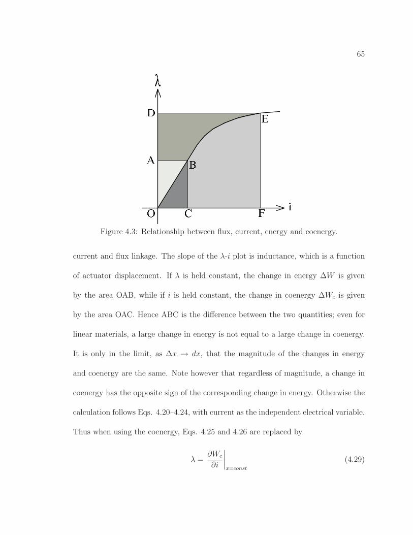
65

Figure 4.3: Relationship between flux, current, energy and coenergy.

current and flux linkage. The slope of the λ-i plot is inductance, which is a function

of actuator displacement. If λ is held constant, the change in energy ∆W is given

by the area OAB, while if i is held constant, the change in coenergy ∆Wc is given

by the area OAC. Hence ABC is the difference between the two quantities; even for

linear materials, a large change in energy is not equal to a large change in coenergy.

It is only in the limit, as ∆x → dx, that the magnitude of the changes in energy

and coenergy are the same. Note however that regardless of magnitude, a change in

coenergy has the opposite sign of the corresponding change in energy. Otherwise the

calculation follows Eqs. 4.20–4.24, with current as the independent electrical variable.

Thus when using the coenergy, Eqs. 4.25 and 4.26 are replaced by

λ =∂Wc

∂i

∣

∣

∣

∣

x=const

(4.29)

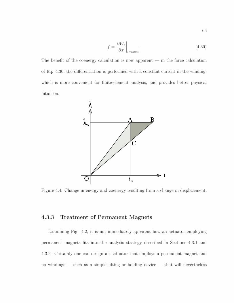
66

f =∂Wc

∂x

∣

∣

∣

∣

i=const

. (4.30)

The benefit of the coenergy calculation is now apparent — in the force calculation

of Eq. 4.30, the differentiation is performed with a constant current in the winding,

which is more convenient for finite-element analysis, and provides better physical

intuition.

Figure 4.4: Change in energy and coenergy resulting from a change in displacement.

4.3.3 Treatment of Permanent Magnets

Examining Fig. 4.2, it is not immediately apparent how an actuator employing

permanent magnets fits into the analysis strategy described in Sections 4.3.1 and

4.3.2. Certainly one can design an actuator that employs a permanent magnet and

no windings — such as a simple lifting or holding device — that will nevertheless

67

develop useful mechanical force. How does the analysis proceed when no external

currents are present?

There are two approaches to the lumped-element analysis. The first, presented in

[70], replaces the magnet with an “equivalent winding” and series reluctance. The

winding MMF is chosen to match that of the magnet

NI = Hcℓmag (4.31)

and the reluctance is determined by the magnet geometry and permeability

R =ℓmag

µrµoAmag

. (4.32)

For most permanent magnet materials, µr falls in the range of 1-10. Consequently,

the coenergy (or energy) within the permanent magnet material is significant, and its

change with displacement must be included in force calculations. With these changes,

analysis can proceed as described in Sec. 4.3.2.

An alternative method for dealing with permanent magnets with arguably more

intuitive appeal is presented in [36]. To allow the problem to fall into the mathematical

framework of Sections 4.3.1 and 4.3.2, a “fictitious” winding is added to the magnetic

circuit in series with the permanent magnet (rather than replacing it). In this way the

MMF of the winding can be chosen to exactly cancel that of the magnet (the value

can be obtained by negating Eq. 4.31). This allows for the zero-force displacement

required by the conceptual development, and introduces a current into the lumped-

element model. The integration in Eq. 4.28 is then carried out starting from a nonzero

68

negative current which ensures zero flux in the gap, to a final value of zero current

(which is the actual operating point of the real device, which has no winding in that

location). Equation 4.28 then becomes

Wc(0, xo) =

∫ i=0

i=−io

λ(i, x)di|x=xo. (4.33)

4.3.4 Treatment of Multiple Windings

It is common for electromechanical actuators to have two, three, or more in-

dependent phases to produce a more constant force or torque, and to ensure that

displacement occurs in the proper direction. These devices may also incorporate per-

manent magnets, adding a number of equivalent or fictitious windings in addition to

real windings. Hence for many applications, the energy or coenergy method analysis

must be extended to account for an arbitrary number of windings. The coenergy

method is developed below; the energy method is similar via the Legendre transform

described in Sec. 4.3.2.

Imagining the black box in Fig. 4.2 with n electrical terminals, an incremental

change in coenergy can be written as

dWc =n∑

k=1

λkdik + fdx (4.34)

69

and hence the coenergy is given as

Wc =

∫ i1=I1

i1=0

λ1(i1, i2=0, . . . , in=0)di1 + . . . (4.35)

+

∫ ik=Ik

ik=0

λk(i1=I1, . . . , ik−1=Ik−1, ik, ik−1=0, . . . , in=0)dik + . . .

+

∫ in=In

in=0

λn(i1=I1, . . . , in−1=In−1, in)din.

For linear systems,

λ1(i1, i2=0, . . . , in=0) = L11i1 (4.36)

λk(i1=I1, . . . , ik−1=Ik−1, ik, ik−1=0, . . . , in=0) = Lk1I1 + . . . + Lkk−1Ikk−1 + Lkkik

λn(i1=I1, . . . , in−1=In−1, in) = Ln1I1 + . . . + Lnn−1Inn−1 + Lnninn

and the integral 4.35 can be written succinctly as

Wc = 12ITLI (4.37)

where L is the inductance matrix whose elements satisfy λj = Ljkik and I is the

corresponding vector of winding currents. Equations 4.29 and 4.30 then apply as

before, where 4.29 is applied to each (λk, ik) pair, and I replaces i in 4.30.

4.3.5 The Energy Method for Distributed Fields

As stated earlier, the energy and coenergy methods can be applied to distributed

field systems as well as lumped element systems. The difference in the distributed

case is that the energy or coenergy is not computed from the terminal quantities λ

70

and i, but rather by computing an energy or coenergy density throughout space, and

integrating this density over the volume in question.

Once again the coenergy analysis will be used due to its greater utility for en-

gineering analysis. However, in theory the energy density could be used as well.

Coenergy density is defined as

W ′c =

∫ H

0

B · dH. (4.38)

Of course B in Eq. 4.38 is a function of H, and the particular function depends on the

material in which the fields are acting. For soft magnetic and nonmagnetic materials

B = µH, and thus

W ′c =

∫ H

0

µH · dH, (4.39)

where µ may be a function of H. For linear materials, i.e. those with constant µ, Eq.

4.39 integrates to

W ′c =

1

2µ|H|2. (4.40)

For hard magnetic materials, recall that

B = µH + Br, (4.41)

and thus

W ′c =

∫ H

0

(µH + Br) · dH. (4.42)

Again assuming a constant µ, Eq. 4.42 integrates to

W ′c =

1

2H2 + Br · H. (4.43)

71

From here, the coenergy can be calculated as

Wc =∑

k

∫

Vk

W ′c dVol, (4.44)

where the integration over each volume Vk in Eq. 4.44 is carried out using an expres-

sion for W ′c appropriate for the material occupying the volume (i.e. Eqs. 4.39, 4.40,

4.42, or 4.43). The resulting expression for Wc can be substituted into Eq. 4.30 to

find force.

4.4 Finite Element Analysis

Finite element analysis (FEA), sometimes referred to as the finite element method

(FEM), is a mathematical tool for obtaining approximate solutions to sophisticated

distributed field problems. (The solutions are approximate in a strict mathemati-

cal sense; in fact FEA is far more accurate than lumped-element techniques.) The

approach is to discretize the problem such that it is amenable to solution with a

computer. A detailed description of FEA is beyond the scope of this work — the

interested reader is referred to [71] or similar works. In this section, a brief overview

of the method is given, along with notes on its application to force calculations for

electromagnetic devices.

72

4.4.1 Calculation of the Finite Element Solution

Finite element analysis begins with the definition of a problem geometry and

boundary conditions, and the generation of a mesh. The geometry is the physical

shape of the device under consideration; material properties such as permeability,

and operating point information such as current density, are typically associated with

various regions of the geometry. Boundary conditions are of three types: “Dirichlet”,

in which the value of the solution vector is held constant; “Neumann”, in which the

derivative of the solution is set to zero; and “periodic” in which a fixed relationship

between two node solutions is specified. In magnetic field problems, the Dirichlet

condition forces magnetic flux lines parallel to the boundary, the Neumann condition

forces flux lines perpendicular to the boundary, and the periodic condition can be

used to model a single pole pair of a multi-pole machine by setting boundaries on

opposite sides of the geometry to be equal.

The mesh is the set of points (called nodes) within the volume of the geometry that

discretizes the problem. The nodes define the vertices of polygons — usually triangles

in 2–D, or tetrahedra in 3–D — which are called the elements. A shape function

is chosen to approximate the solution over the area (or volume) of each element.

Linear or quadratic functions of the spatial variables suffice for many problems. The

coefficients of this polynomial can then be determined in terms of the node values,

and hence a closed-form expression exists for the solution within each element.

73

A scalar expression for the difference between energy stored in the field (expressed

as the integral of H with respect to B) and energy delivered to the system (expressed

as the integral of J with respect to A) is developed for each element. The sum of

the value of this expression over all the elements is called an energy functional, and

for the exact field solution its value is zero. However, because the shape function

is in general only an approximation, the “best fit” solution is that which drives the

energy functional closest to zero. Hence the essence of finite element analysis is the

minimization of this functional.

The finite-element solution for magneto-quasistatic problems is given in terms of

the magnetic potential vector A. The flux density B can then be reconstructed from

the definition

B = ∇× A, (4.45)

and H then determined from Eq. 4.10 or Eq. 4.41 as appropriate.

4.4.2 Force Calculations

The strategy for force or torque calculation via FEA follows Sec. 4.3.5, with the

volume integral in Eq. 4.44 replaced by a summation over the elements:

Wc = ΣkW′c[k] · V ol[k]. (4.46)

For each displacement at which the force is to be determined, the finite-element

solution and coenergy must be calculated twice: once at a small negative perturbation

74

ǫ from the point of interest; and once at a small positive perturbation. The two

displacements and two coenergy values can then be used to approximate the force via

a numerical differential:

F (xo) =Wc(xo+ǫ) − Wc(xo−ǫ)

(xo+ǫ) − (xo−ǫ)=

∆Wc

2ǫ. (4.47)

The fact that two solutions must be calculated for each displacement, and that each

solution can require significant computation time (on the order of minutes to hours

with modest computing resources), limits the utility of FEA for design synthesis or

optimization, in which many solutions are desired quickly.

4.5 A Comparison of Various Analysis Methods

Here the analyses described in Secs. 4.2-4.4 are performed for a simple test struc-

ture. The purpose of this section is to provide practical detail to support the theoret-

ical calculations above, as well as to highlight some of the advantages and drawbacks

of the various methods.

The test structure is shown in Fig. 4.5. This is an extremely simple device in

which a permanent magnet and soft magnetic yoke apply force to a soft magnetic

sliding element which is constrained to move only in the horizontal direction. The

winding is a “fictitious winding”, as described in Sec. 4.3.3, which is not part of the

actuator structure but rather a conceptual tool that will be required for the analysis

in some of the sections below. The structure has uniform thickness, and uniform

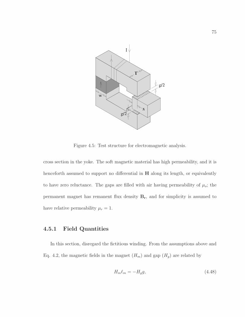
75

Figure 4.5: Test structure for electromagnetic analysis.

cross section in the yoke. The soft magnetic material has high permeability, and it is

henceforth assumed to support no differential in H along its length, or equivalently

to have zero reluctance. The gaps are filled with air having permeability of µo; the

permanent magnet has remanent flux density Br, and for simplicity is assumed to

have relative permeability µr = 1.

4.5.1 Field Quantities

In this section, disregard the fictitious winding. From the assumptions above and

Eq. 4.2, the magnetic fields in the magnet (Hm) and gap (Hg) are related by

Hmℓm = −Hgg, (4.48)

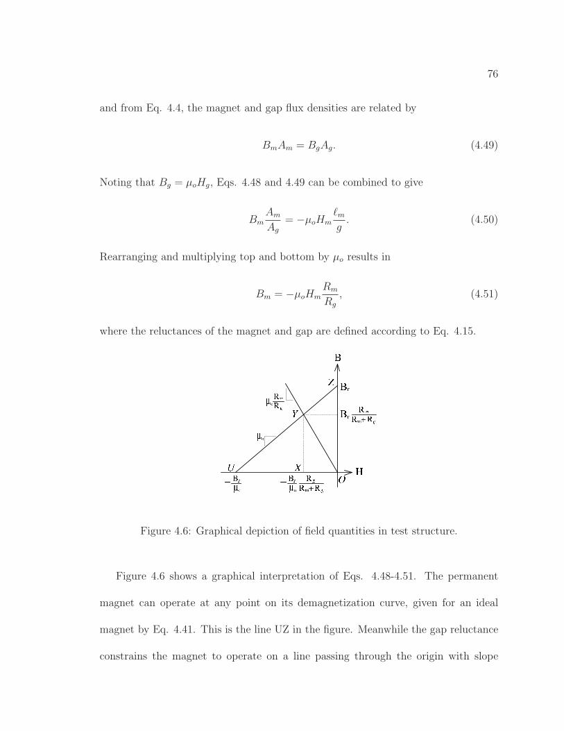
76

and from Eq. 4.4, the magnet and gap flux densities are related by

BmAm = BgAg. (4.49)

Noting that Bg = µoHg, Eqs. 4.48 and 4.49 can be combined to give

Bm

Am

Ag

= −µoHm

ℓm

g. (4.50)

Rearranging and multiplying top and bottom by µo results in

Bm = −µoHm

Rm

Rg

, (4.51)

where the reluctances of the magnet and gap are defined according to Eq. 4.15.

Figure 4.6: Graphical depiction of field quantities in test structure.

Figure 4.6 shows a graphical interpretation of Eqs. 4.48-4.51. The permanent

magnet can operate at any point on its demagnetization curve, given for an ideal

magnet by Eq. 4.41. This is the line UZ in the figure. Meanwhile the gap reluctance

constrains the magnet to operate on a line passing through the origin with slope

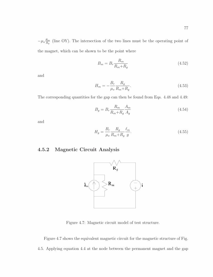
77

−µoRm

Rg(line OY). The intersection of the two lines must be the operating point of

the magnet, which can be shown to be the point where

Bm = Br

Rm

Rm+Rg

(4.52)

and

Hm = −Br

µo

Rg

Rm+Rg

. (4.53)

The corresponding quantities for the gap can then be found from Eqs. 4.48 and 4.49:

Bg = Br

Rm

Rm+Rg

Am

Ag

(4.54)

and

Hg =Br

µo

Rg

Rm+Rg

ℓm

g. (4.55)

4.5.2 Magnetic Circuit Analysis

Figure 4.7: Magnetic circuit model of test structure.

Figure 4.7 shows the equivalent magnetic circuit for the magnetic structure of Fig.

4.5. Applying equation 4.4 at the node between the permanent magnet and the gap

78

reluctance gives

λm = λo − λg (4.56)

where λo is the flux linkage corresponding to Br, λm is the leakage flux across the

magnet, and λg is the flux that crosses the gap. Summing MMFs around the loop

gives

λmRm − λgRg + i = 0. (4.57)

Substituting in Eq. 4.56 then gives the gap flux, in terms of the magnet remanent

flux and the current in the fictitious winding:

λg = λ0Rm

Rm+Rg

+ i1

Rm+Rg

(4.58)

4.5.3 Coenergy Calculation Via Fictitious Winding

To find the coenergy using the magnetic circuit model and the fictitious winding

method, Eq. 4.33 is applied. Recall that the integration of flux linkage with respect

to current is carried out from a starting current that ensures zero flux in the gap, in

this case io = −λoRm (by inspection of Eq. 4.58). Thus

Wc =

∫ 0

−λoRm

λg(i)di =

∫ 0

−λoRm

λ0Rm

Rm+Rg

+ i1

Rm+Rg

di, (4.59)

which evaluates to

Wc =1

2

(λoRm)2

Rm+Rg

. (4.60)

79

4.5.4 Coenergy Calculation Via Equivalent Winding

The alternative to the fictitious winding method, as discussed in Sec. 4.3.3, is

to simply replace the permanent magnet, for purposes of analysis, with a Thevenin

equivalent winding and series reluctance. In this case the fictitious winding is not

necessary. The Thevenin equivalent winding carries current i = λoRm, and the series

reluctance is simply Rm = ℓm

µoAm. The coenergy is calculated by integrating the flux

linking the equivalent winding with respect to current:

Wc =

∫ λoRm

0

λg(i)di =

∫ λoRm

0

i

Rm+Rg

di. (4.61)

Equation 4.61 evaluates, as expected, to

Wc =1

2

(λoRm)2

Rm+Rg

. (4.62)

4.5.5 Coenergy Calculation Via Coenergy Density

The coenergy can also be calculated by first finding the coenergy density in a

particular region, and then integrating over the volume of the region as discussed

in Sec. 4.3.5. In the case of a structure with permanent magnets, a large portion

of the coenergy can be contained within the magnet volume, and hence this volume

must be included in the calculation. Recalling Eq. 4.38, the coenergy density in the

permanent magnet can be found by substituting in Eq. 4.41:

W ′c,pm =

∫ Hm

0

(Br + µoH)dH = (Br · Hm) +1

2µo|Hm|2. (4.63)

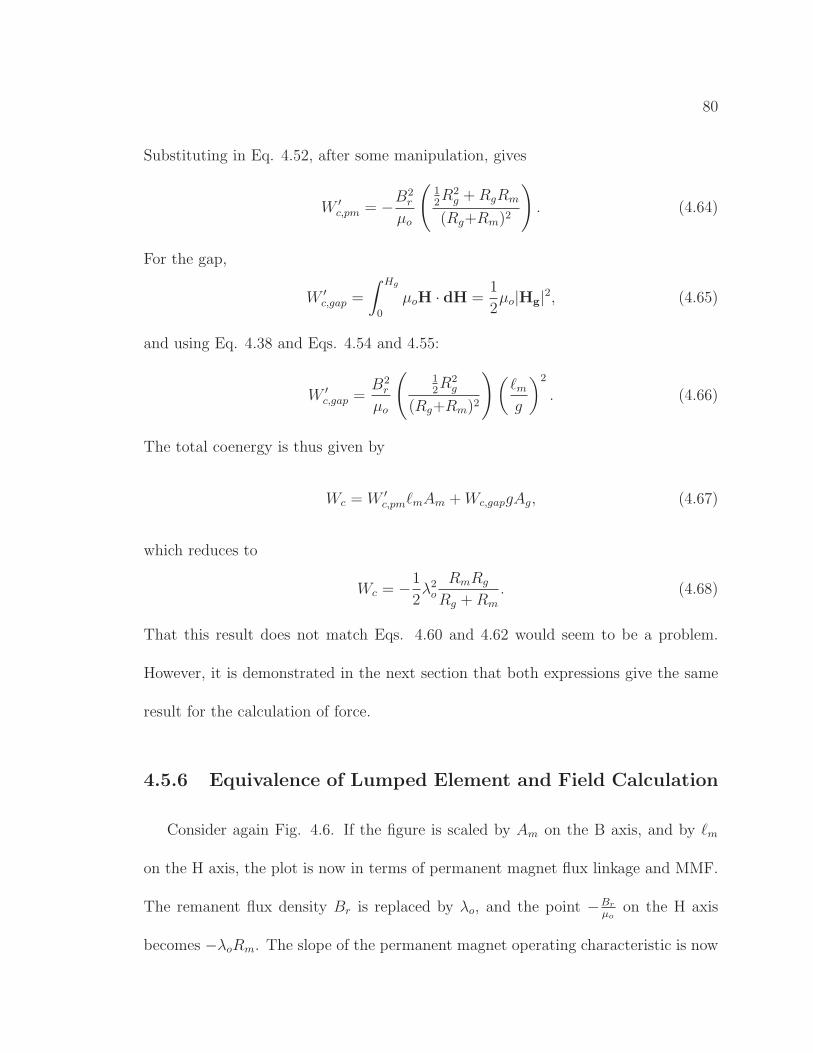
80

Substituting in Eq. 4.52, after some manipulation, gives

W ′c,pm = −B2

r

µo

(

12R2

g + RgRm

(Rg+Rm)2

)

. (4.64)

For the gap,

W ′c,gap =

∫ Hg

0

µoH · dH =1

2µo|Hg|2, (4.65)

and using Eq. 4.38 and Eqs. 4.54 and 4.55:

W ′c,gap =

B2r

µo

(

12R2

g

(Rg+Rm)2

)

(

ℓm

g

)2

. (4.66)

The total coenergy is thus given by

Wc = W ′c,pmℓmAm + Wc,gapgAg, (4.67)

which reduces to

Wc = −1

2λ2

o

RmRg

Rg + Rm

. (4.68)

That this result does not match Eqs. 4.60 and 4.62 would seem to be a problem.

However, it is demonstrated in the next section that both expressions give the same

result for the calculation of force.

4.5.6 Equivalence of Lumped Element and Field Calculation

Consider again Fig. 4.6. If the figure is scaled by Am on the B axis, and by ℓm

on the H axis, the plot is now in terms of permanent magnet flux linkage and MMF.

The remanent flux density Br is replaced by λo, and the point −Br

µoon the H axis

becomes −λoRm. The slope of the permanent magnet operating characteristic is now

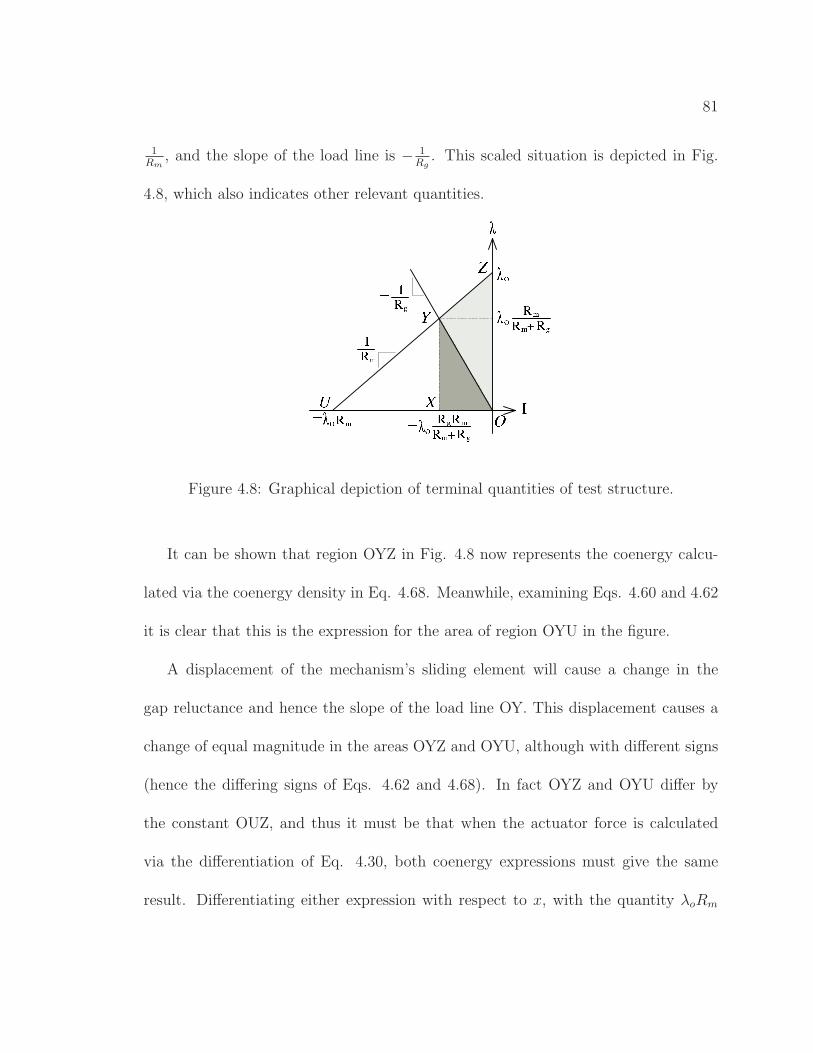
81

1Rm

, and the slope of the load line is − 1Rg

. This scaled situation is depicted in Fig.

4.8, which also indicates other relevant quantities.

Figure 4.8: Graphical depiction of terminal quantities of test structure.

It can be shown that region OYZ in Fig. 4.8 now represents the coenergy calcu-

lated via the coenergy density in Eq. 4.68. Meanwhile, examining Eqs. 4.60 and 4.62

it is clear that this is the expression for the area of region OYU in the figure.

A displacement of the mechanism’s sliding element will cause a change in the

gap reluctance and hence the slope of the load line OY. This displacement causes a

change of equal magnitude in the areas OYZ and OYU, although with different signs

(hence the differing signs of Eqs. 4.62 and 4.68). In fact OYZ and OYU differ by

the constant OUZ, and thus it must be that when the actuator force is calculated

via the differentiation of Eq. 4.30, both coenergy expressions must give the same

result. Differentiating either expression with respect to x, with the quantity λoRm

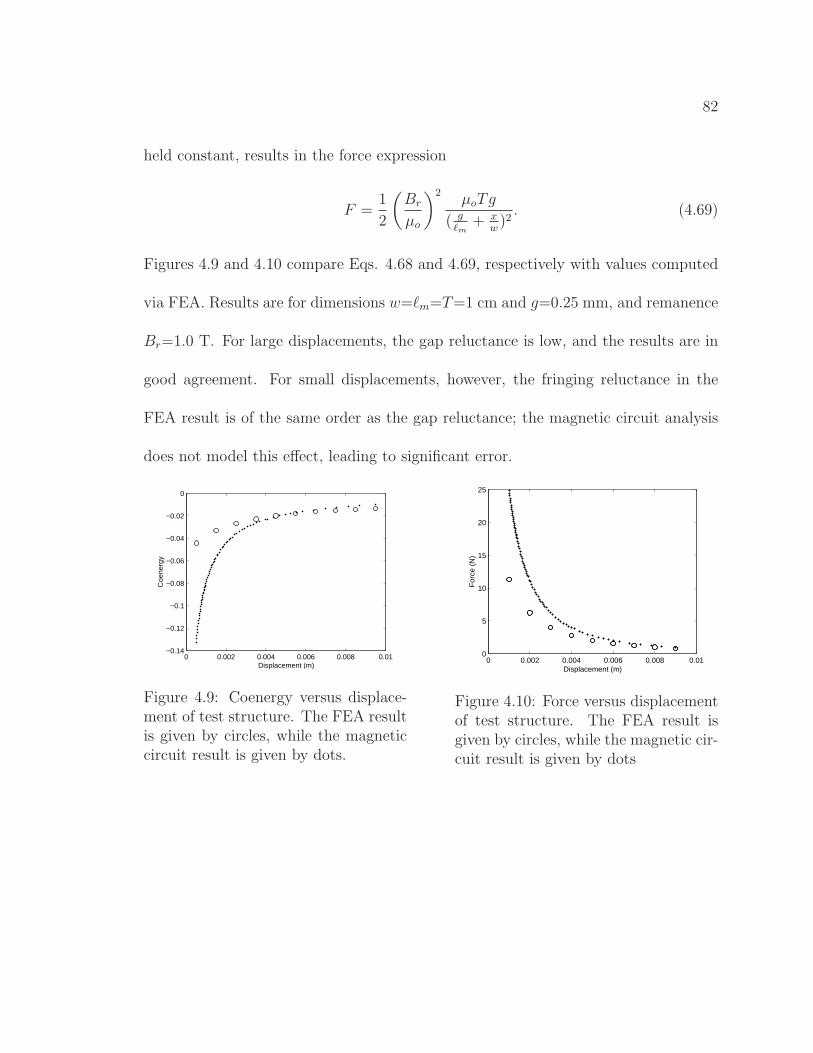
82

held constant, results in the force expression

F =1

2

(

Br

µo

)2µoTg

( gℓm

+ xw)2

. (4.69)

Figures 4.9 and 4.10 compare Eqs. 4.68 and 4.69, respectively with values computed

via FEA. Results are for dimensions w=ℓm=T=1 cm and g=0.25 mm, and remanence

Br=1.0 T. For large displacements, the gap reluctance is low, and the results are in

good agreement. For small displacements, however, the fringing reluctance in the

FEA result is of the same order as the gap reluctance; the magnetic circuit analysis

does not model this effect, leading to significant error.

0 0.002 0.004 0.006 0.008 0.01−0.14

−0.12

−0.1

−0.08

−0.06

−0.04

−0.02

0

Displacement (m)

Coe

nerg

y

Figure 4.9: Coenergy versus displace-ment of test structure. The FEA resultis given by circles, while the magneticcircuit result is given by dots.

0 0.002 0.004 0.006 0.008 0.010

5

10

15

20

25

Displacement (m)

For

ce (

N)

Figure 4.10: Force versus displacementof test structure. The FEA result isgiven by circles, while the magnetic cir-cuit result is given by dots

83

Chapter 5

Machine Design and Analysis —

Millimeter Scale

This chapter describes the design, construction and testing of a millimeter-scale

electromagnetic generator intended to be coupled to a MEMS internal combustion

engine. The novel configuration of the machine posed several challenges to analysis

which are described in Sec. 5.2. The machine’s configuration as well as its size —

small for the macro-scale, large for the micro-scale — introduced some construction

issues, as detailed in Sec. 5.3. Experimental results are presented in Sec. 5.4.

5.1 Design

The generator configuration shown in Figs. 5.1 and 5.2 was developed in response

to two major constraints: the unusual Wankel rotor geometry, which is not well

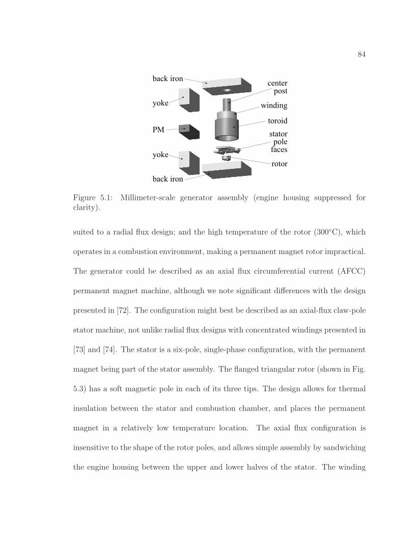
84

rotor

winding

PMstator

polefaces

back iron

back iron

centerpost

yoke

yoke

toroid

Figure 5.1: Millimeter-scale generator assembly (engine housing suppressed forclarity).

suited to a radial flux design; and the high temperature of the rotor (300C), which

operates in a combustion environment, making a permanent magnet rotor impractical.

The generator could be described as an axial flux circumferential current (AFCC)

permanent magnet machine, although we note significant differences with the design

presented in [72]. The configuration might best be described as an axial-flux claw-pole

stator machine, not unlike radial flux designs with concentrated windings presented in

[73] and [74]. The stator is a six-pole, single-phase configuration, with the permanent

magnet being part of the stator assembly. The flanged triangular rotor (shown in Fig.

5.3) has a soft magnetic pole in each of its three tips. The design allows for thermal

insulation between the stator and combustion chamber, and places the permanent

magnet in a relatively low temperature location. The axial flux configuration is

insensitive to the shape of the rotor poles, and allows simple assembly by sandwiching

the engine housing between the upper and lower halves of the stator. The winding

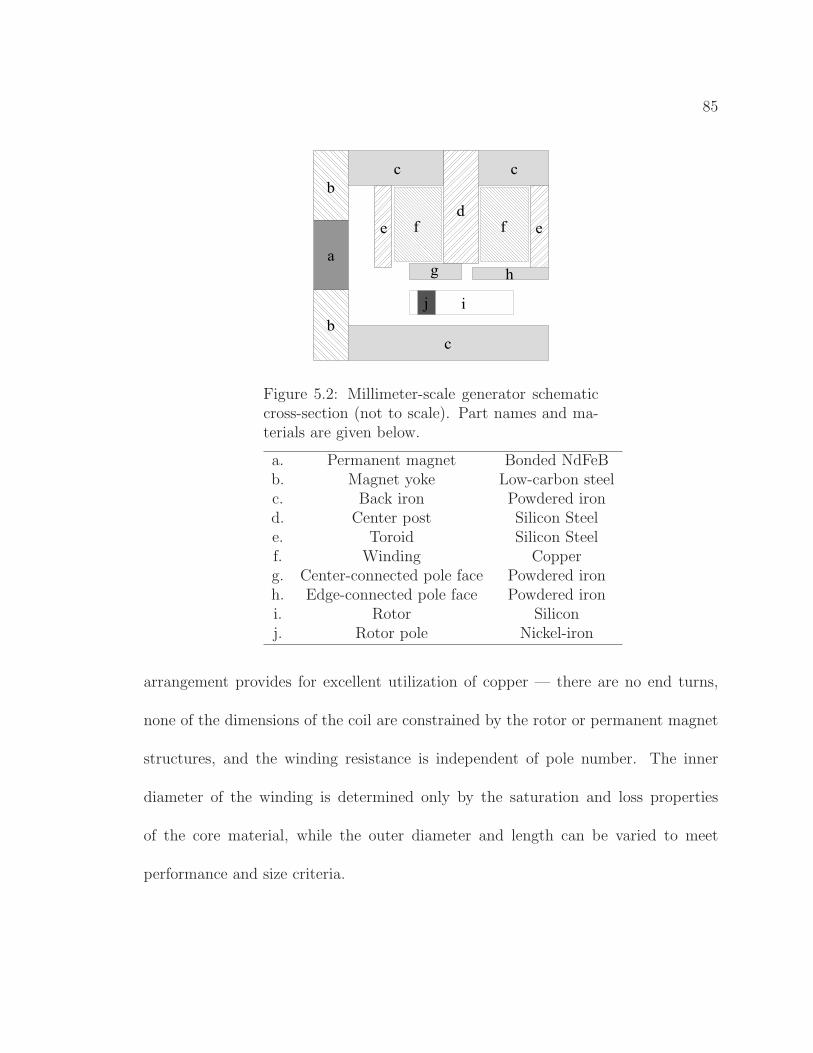
85

a

b

b

c c

c

de ef f

g h

ij

Figure 5.2: Millimeter-scale generator schematiccross-section (not to scale). Part names and ma-terials are given below.

a. Permanent magnet Bonded NdFeBb. Magnet yoke Low-carbon steelc. Back iron Powdered irond. Center post Silicon Steele. Toroid Silicon Steelf. Winding Copperg. Center-connected pole face Powdered ironh. Edge-connected pole face Powdered ironi. Rotor Siliconj. Rotor pole Nickel-iron

arrangement provides for excellent utilization of copper — there are no end turns,

none of the dimensions of the coil are constrained by the rotor or permanent magnet

structures, and the winding resistance is independent of pole number. The inner

diameter of the winding is determined only by the saturation and loss properties

of the core material, while the outer diameter and length can be varied to meet

performance and size criteria.

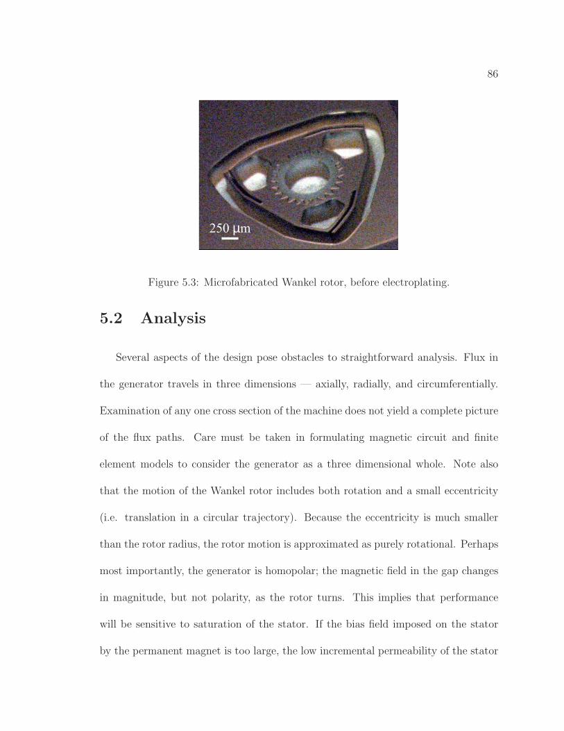
86

250 µm

Figure 5.3: Microfabricated Wankel rotor, before electroplating.

5.2 Analysis

Several aspects of the design pose obstacles to straightforward analysis. Flux in

the generator travels in three dimensions — axially, radially, and circumferentially.

Examination of any one cross section of the machine does not yield a complete picture

of the flux paths. Care must be taken in formulating magnetic circuit and finite

element models to consider the generator as a three dimensional whole. Note also

that the motion of the Wankel rotor includes both rotation and a small eccentricity

(i.e. translation in a circular trajectory). Because the eccentricity is much smaller

than the rotor radius, the rotor motion is approximated as purely rotational. Perhaps

most importantly, the generator is homopolar; the magnetic field in the gap changes

in magnitude, but not polarity, as the rotor turns. This implies that performance

will be sensitive to saturation of the stator. If the bias field imposed on the stator

by the permanent magnet is too large, the low incremental permeability of the stator

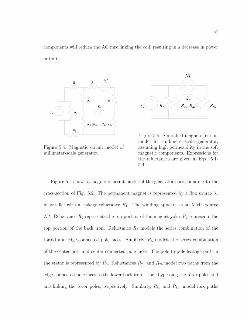
87

components will reduce the AC flux linking the coil, resulting in a decrease in power

output.

NI

R4

R6

R7a

R5

R10

R2

R9

R3

||R7b R8a||R8b

Figure 5.4: Magnetic circuit model ofmillimeter-scale generator.

NI

R7bR7a R8a R8bx

w

Figure 5.5: Simplified magnetic circuitmodel for millimeter-scale generator,assuming high permeability in the softmagnetic components. Expressions forthe reluctances are given in Eqs. 5.1-5.4

Figure 5.4 shows a magnetic circuit model of the generator corresponding to the

cross-section of Fig. 5.2. The permanent magnet is represented by a flux source λo

in parallel with a leakage reluctance R1. The winding appears as an MMF source

NI. Reluctance R2 represents the top portion of the magnet yoke; R3 represents the

top portion of the back iron. Reluctance R4 models the series combination of the

toroid and edge-connected pole faces. Similarly, R5 models the series combination

of the center post and center-connected pole faces. The pole to pole leakage path in

the stator is represented by R6. Reluctances R7a and R7b model two paths from the

edge-connected pole faces to the lower back iron — one bypassing the rotor poles and

one linking the rotor poles, respectively. Similarly, R8a and R8b, model flux paths

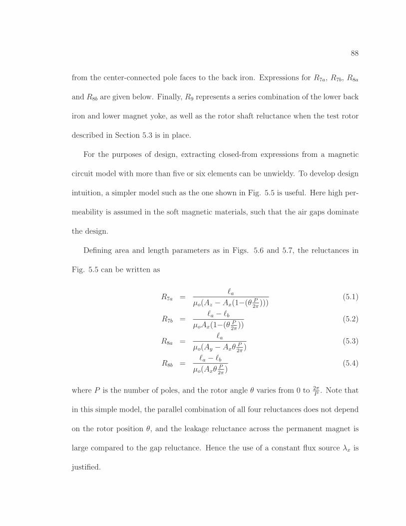
88

from the center-connected pole faces to the back iron. Expressions for R7a, R7b, R8a

and R8b are given below. Finally, R9 represents a series combination of the lower back

iron and lower magnet yoke, as well as the rotor shaft reluctance when the test rotor

described in Section 5.3 is in place.

For the purposes of design, extracting closed-from expressions from a magnetic

circuit model with more than five or six elements can be unwieldy. To develop design

intuition, a simpler model such as the one shown in Fig. 5.5 is useful. Here high per-

meability is assumed in the soft magnetic materials, such that the air gaps dominate

the design.

Defining area and length parameters as in Figs. 5.6 and 5.7, the reluctances in

Fig. 5.5 can be written as

R7a =ℓa

µo(Az − Ax(1−(θ P2π

)))(5.1)

R7b =ℓa − ℓb

µoAx(1−(θ P2π

))(5.2)

R8a =ℓa

µo(Ay − AxθP2π

)(5.3)

R8b =ℓa − ℓb

µo(AxθP2π

)(5.4)

where P is the number of poles, and the rotor angle θ varies from 0 to 2πP

. Note that

in this simple model, the parallel combination of all four reluctances does not depend

on the rotor position θ, and the leakage reluctance across the permanent magnet is

large compared to the gap reluctance. Hence the use of a constant flux source λx is

justified.

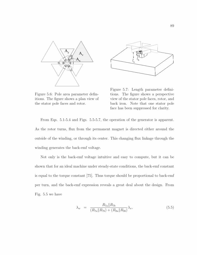
89

Az

Ax

Ay

Figure 5.6: Pole area parameter defin-itions. The figure shows a plan view ofthe stator pole faces and rotor.

la

lb

Figure 5.7: Length parameter defini-tions. The figure shows a perspectiveview of the stator pole faces, rotor, andback iron. Note that one stator poleface has been suppressed for clarity.

From Eqs. 5.1-5.4 and Figs. 5.5-5.7, the operation of the generator is apparent.

As the rotor turns, flux from the permanent magnet is directed either around the

outside of the winding, or through its center. This changing flux linkage through the

winding generates the back-emf voltage.

Not only is the back-emf voltage intuitive and easy to compute, but it can be

shown that for an ideal machine under steady-state conditions, the back-emf constant

is equal to the torque constant [75]. Thus torque should be proportional to back-emf

per turn, and the back-emf expression reveals a great deal about the design. From

Fig. 5.5 we have

λw =R7a‖R7b

(R7a‖R7b) + (R8a‖R8b)λx, (5.5)

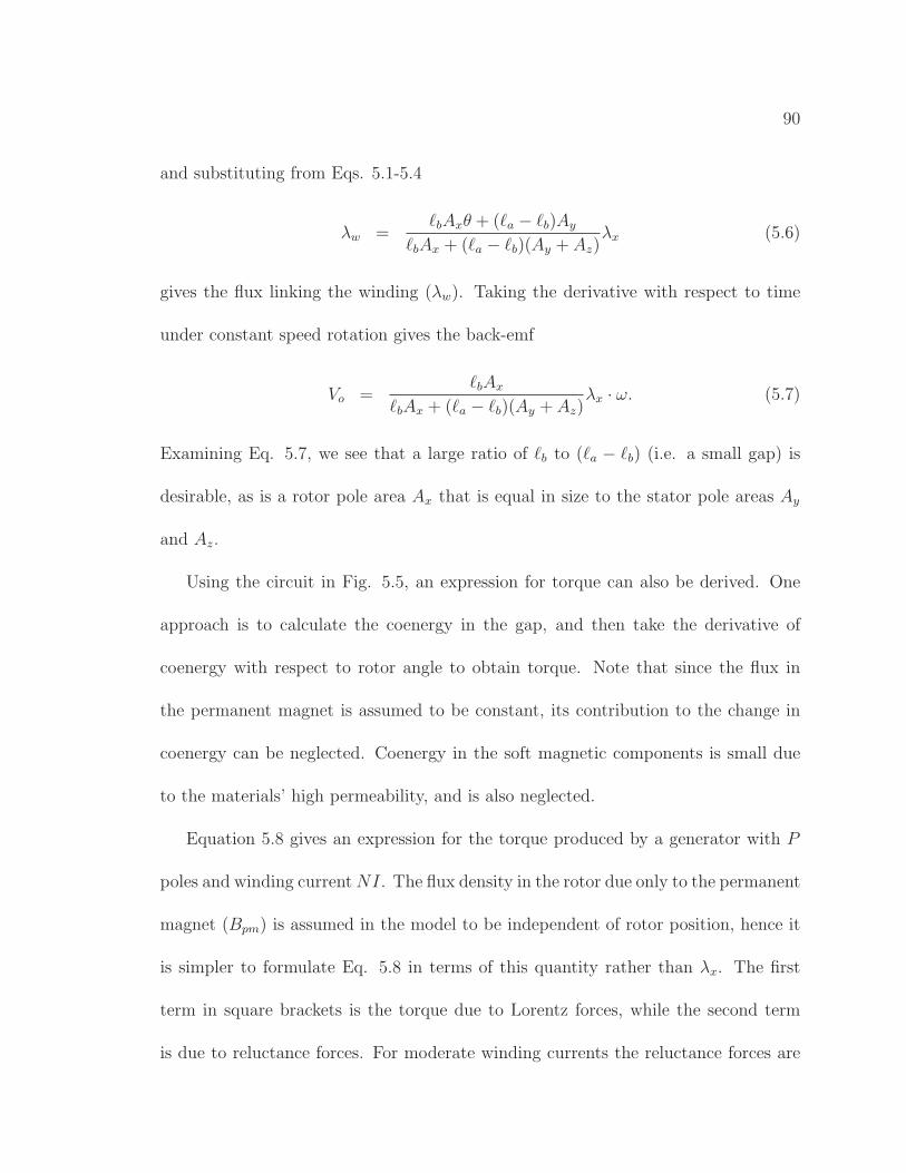
90

and substituting from Eqs. 5.1-5.4

λw =ℓbAxθ + (ℓa − ℓb)Ay

ℓbAx + (ℓa − ℓb)(Ay + Az)λx (5.6)

gives the flux linking the winding (λw). Taking the derivative with respect to time

under constant speed rotation gives the back-emf

Vo =ℓbAx

ℓbAx + (ℓa − ℓb)(Ay + Az)λx · ω. (5.7)

Examining Eq. 5.7, we see that a large ratio of ℓb to (ℓa − ℓb) (i.e. a small gap) is

desirable, as is a rotor pole area Ax that is equal in size to the stator pole areas Ay

and Az.

Using the circuit in Fig. 5.5, an expression for torque can also be derived. One

approach is to calculate the coenergy in the gap, and then take the derivative of

coenergy with respect to rotor angle to obtain torque. Note that since the flux in

the permanent magnet is assumed to be constant, its contribution to the change in

coenergy can be neglected. Coenergy in the soft magnetic components is small due

to the materials’ high permeability, and is also neglected.

Equation 5.8 gives an expression for the torque produced by a generator with P

poles and winding current NI. The flux density in the rotor due only to the permanent

magnet (Bpm) is assumed in the model to be independent of rotor position, hence it

is simpler to formulate Eq. 5.8 in terms of this quantity rather than λx. The first

term in square brackets is the torque due to Lorentz forces, while the second term

is due to reluctance forces. For moderate winding currents the reluctance forces are

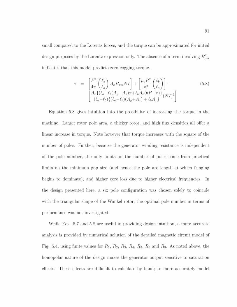
91

small compared to the Lorentz forces, and the torque can be approximated for initial

design purposes by the Lorentz expression only. The absence of a term involving B2pm

indicates that this model predicts zero cogging torque.

τ =

[

P 2

4π

(

ℓb

ℓa

)

AxBpmNI

]

+

[

µoP2

π2

(

ℓb

ℓa

)]

· (5.8)

[

Ax(ℓa−ℓb(Ay−Az)π+ℓbAx(θP−π)(ℓa−ℓb)(ℓa−ℓb)(Ay+Az) + ℓbAx

(NI)2

]

Equation 5.8 gives intuition into the possibility of increasing the torque in the

machine. Larger rotor pole area, a thicker rotor, and high flux densities all offer a

linear increase in torque. Note however that torque increases with the square of the

number of poles. Further, because the generator winding resistance is independent

of the pole number, the only limits on the number of poles come from practical

limits on the minimum gap size (and hence the pole arc length at which fringing

begins to dominate), and higher core loss due to higher electrical frequencies. In

the design presented here, a six pole configuration was chosen solely to coincide

with the triangular shape of the Wankel rotor; the optimal pole number in terms of

performance was not investigated.

While Eqs. 5.7 and 5.8 are useful in providing design intuition, a more accurate

analysis is provided by numerical solution of the detailed magnetic circuit model of

Fig. 5.4, using finite values for R1, R2, R3, R4, R5, R6 and R9. As noted above, the

homopolar nature of the design makes the generator output sensitive to saturation

effects. These effects are difficult to calculate by hand; to more accurately model

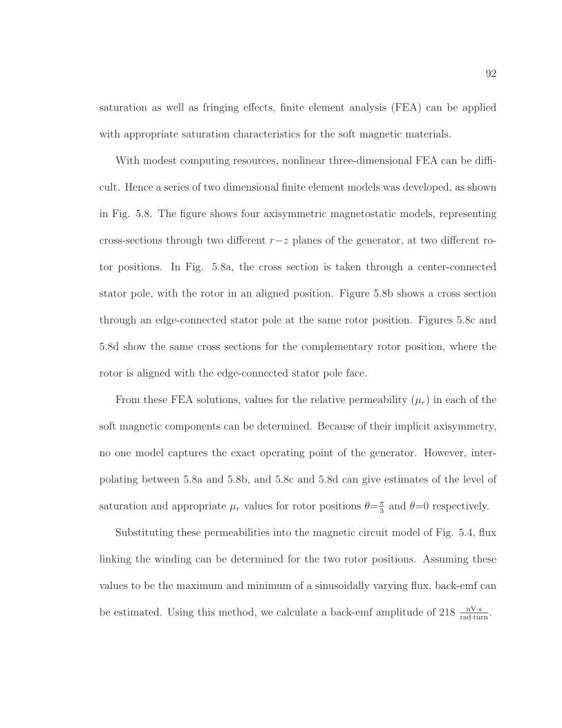
92

saturation as well as fringing effects, finite element analysis (FEA) can be applied

with appropriate saturation characteristics for the soft magnetic materials.

With modest computing resources, nonlinear three-dimensional FEA can be diffi-

cult. Hence a series of two dimensional finite element models was developed, as shown

in Fig. 5.8. The figure shows four axisymmetric magnetostatic models, representing

cross-sections through two different r−z planes of the generator, at two different ro-

tor positions. In Fig. 5.8a, the cross section is taken through a center-connected

stator pole, with the rotor in an aligned position. Figure 5.8b shows a cross section

through an edge-connected stator pole at the same rotor position. Figures 5.8c and

5.8d show the same cross sections for the complementary rotor position, where the

rotor is aligned with the edge-connected stator pole face.

From these FEA solutions, values for the relative permeability (µr) in each of the

soft magnetic components can be determined. Because of their implicit axisymmetry,

no one model captures the exact operating point of the generator. However, inter-

polating between 5.8a and 5.8b, and 5.8c and 5.8d can give estimates of the level of

saturation and appropriate µr values for rotor positions θ=π3

and θ=0 respectively.

Substituting these permeabilities into the magnetic circuit model of Fig. 5.4, flux

linking the winding can be determined for the two rotor positions. Assuming these

values to be the maximum and minimum of a sinusoidally varying flux, back-emf can

be estimated. Using this method, we calculate a back-emf amplitude of 218 nV·srad·turn

.

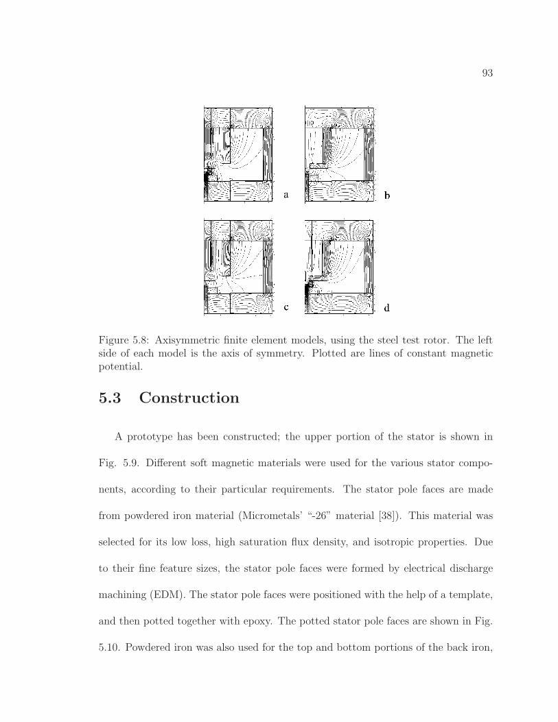
93

Figure 5.8: Axisymmetric finite element models, using the steel test rotor. The leftside of each model is the axis of symmetry. Plotted are lines of constant magneticpotential.

5.3 Construction

A prototype has been constructed; the upper portion of the stator is shown in

Fig. 5.9. Different soft magnetic materials were used for the various stator compo-

nents, according to their particular requirements. The stator pole faces are made

from powdered iron material (Micrometals’ “-26” material [38]). This material was

selected for its low loss, high saturation flux density, and isotropic properties. Due

to their fine feature sizes, the stator pole faces were formed by electrical discharge

machining (EDM). The stator pole faces were positioned with the help of a template,

and then potted together with epoxy. The potted stator pole faces are shown in Fig.

5.10. Powdered iron was also used for the top and bottom portions of the back iron,

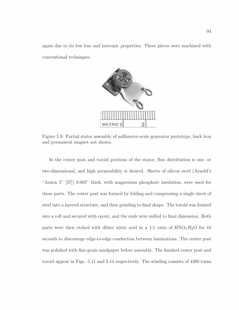
94

again due to its low loss and isotropic properties. These pieces were machined with

conventional techniques.

Figure 5.9: Partial stator assembly of millimeter-scale generator prototype, back ironand permanent magnet not shown.

In the center post and toroid portions of the stator, flux distribution is one- or

two-dimensional, and high permeability is desired. Sheets of silicon steel (Arnold’s

“Arnon 5” [37]) 0.005” thick, with magnesium phosphate insulation, were used for

these parts. The center post was formed by folding and compressing a single sheet of

steel into a layered structure, and then grinding to final shape. The toroid was formed

into a roll and secured with epoxy, and the ends were milled to final dimension. Both

parts were then etched with dilute nitric acid in a 1:1 ratio of HNO3:H2O for 10

seconds to discourage edge-to-edge conduction between laminations. The center post

was polished with fine-grain sandpaper before assembly. The finished center post and

toroid appear in Figs. 5.11 and 5.14 respectively. The winding consists of 4200 turns

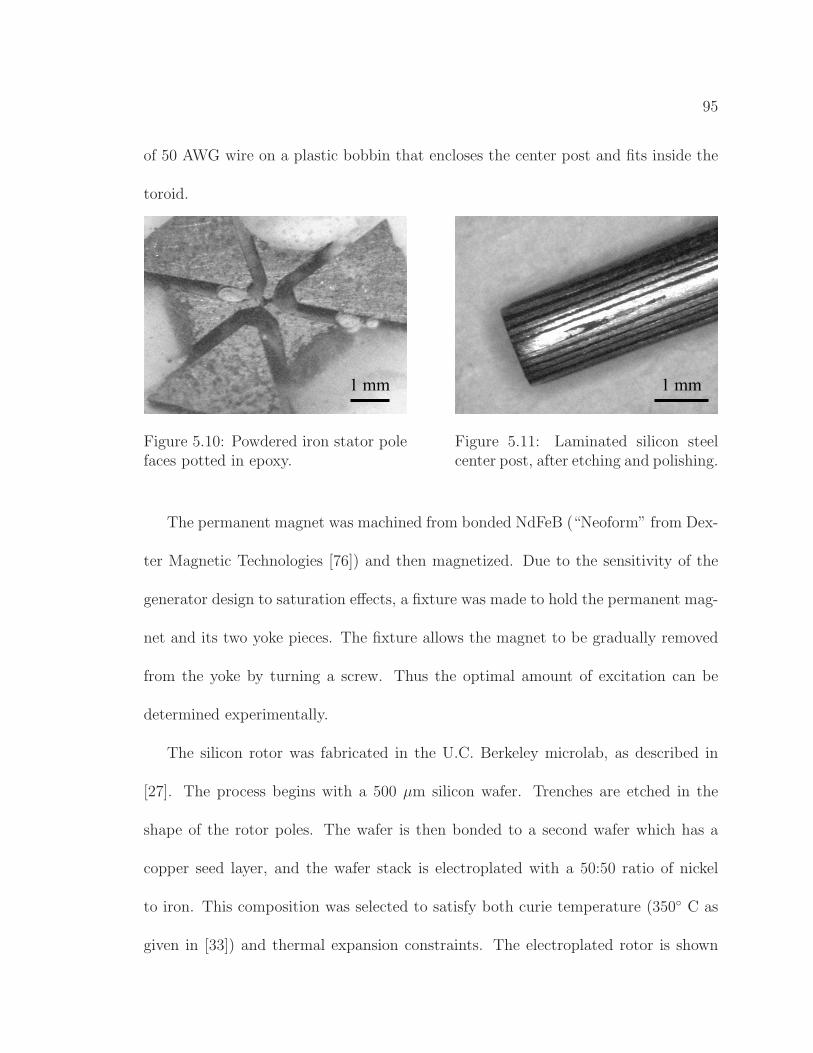
95

of 50 AWG wire on a plastic bobbin that encloses the center post and fits inside the

toroid.

1 mm

Figure 5.10: Powdered iron stator polefaces potted in epoxy.

1 mm

Figure 5.11: Laminated silicon steelcenter post, after etching and polishing.

The permanent magnet was machined from bonded NdFeB (“Neoform” from Dex-

ter Magnetic Technologies [76]) and then magnetized. Due to the sensitivity of the

generator design to saturation effects, a fixture was made to hold the permanent mag-

net and its two yoke pieces. The fixture allows the magnet to be gradually removed

from the yoke by turning a screw. Thus the optimal amount of excitation can be

determined experimentally.

The silicon rotor was fabricated in the U.C. Berkeley microlab, as described in

[27]. The process begins with a 500 µm silicon wafer. Trenches are etched in the

shape of the rotor poles. The wafer is then bonded to a second wafer which has a

copper seed layer, and the wafer stack is electroplated with a 50:50 ratio of nickel

to iron. This composition was selected to satisfy both curie temperature (350 C as

given in [33]) and thermal expansion constraints. The electroplated rotor is shown

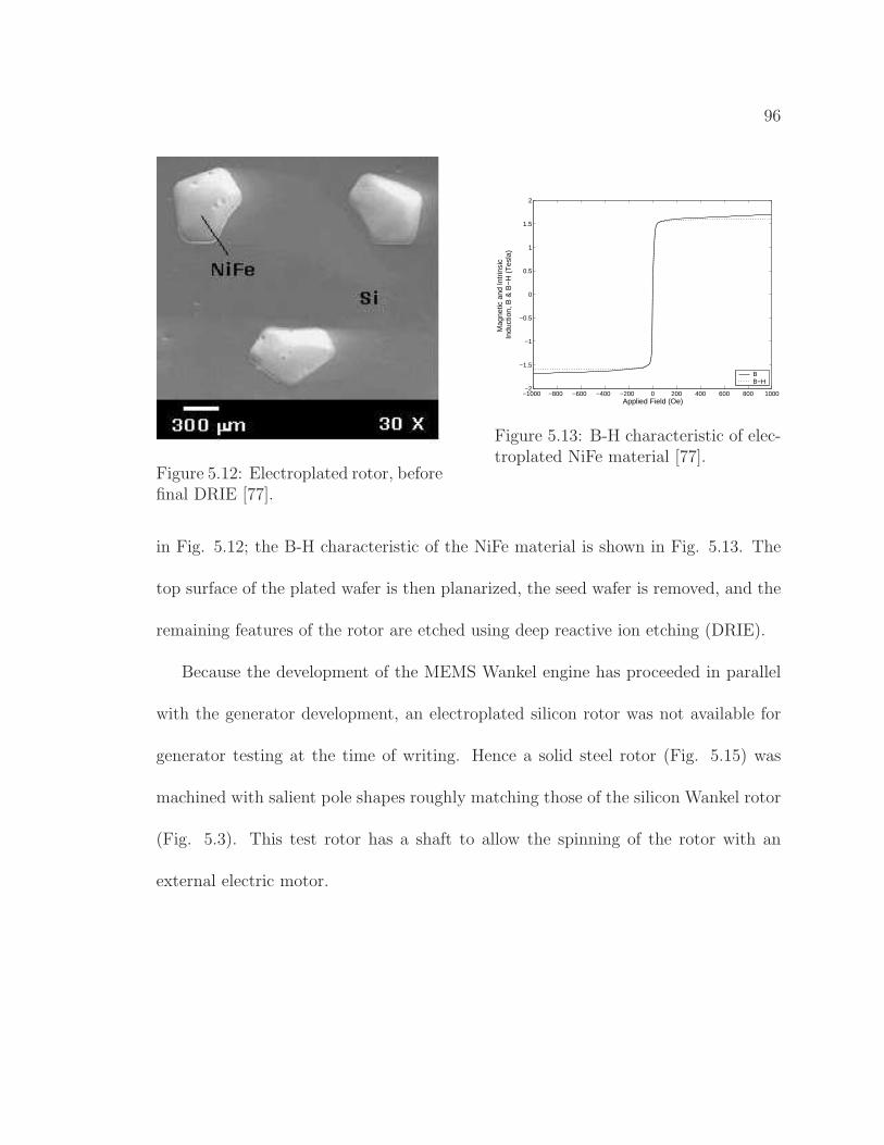
96

Figure 5.12: Electroplated rotor, beforefinal DRIE [77].

−1000 −800 −600 −400 −200 0 200 400 600 800 1000−2

−1.5

−1

−0.5

0

0.5

1

1.5

2

Applied Field (Oe)

Mag

netic

and

Intr

insi

c In

duct

ion,

B &

B−

H (

Tes

la)

B B−H

Figure 5.13: B-H characteristic of elec-troplated NiFe material [77].

in Fig. 5.12; the B-H characteristic of the NiFe material is shown in Fig. 5.13. The

top surface of the plated wafer is then planarized, the seed wafer is removed, and the

remaining features of the rotor are etched using deep reactive ion etching (DRIE).

Because the development of the MEMS Wankel engine has proceeded in parallel

with the generator development, an electroplated silicon rotor was not available for

generator testing at the time of writing. Hence a solid steel rotor (Fig. 5.15) was

machined with salient pole shapes roughly matching those of the silicon Wankel rotor

(Fig. 5.3). This test rotor has a shaft to allow the spinning of the rotor with an

external electric motor.

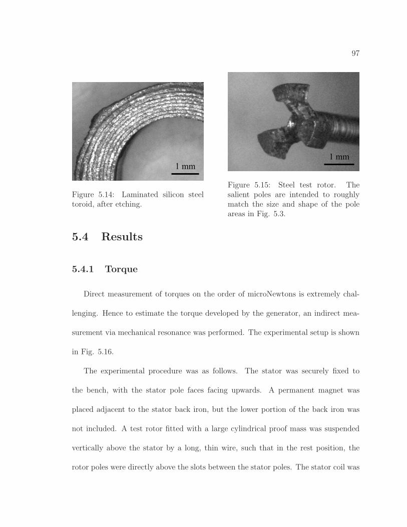
97

1 mm

Figure 5.14: Laminated silicon steeltoroid, after etching.

1 mm

Figure 5.15: Steel test rotor. Thesalient poles are intended to roughlymatch the size and shape of the poleareas in Fig. 5.3.

5.4 Results

5.4.1 Torque

Direct measurement of torques on the order of microNewtons is extremely chal-

lenging. Hence to estimate the torque developed by the generator, an indirect mea-

surement via mechanical resonance was performed. The experimental setup is shown

in Fig. 5.16.

The experimental procedure was as follows. The stator was securely fixed to

the bench, with the stator pole faces facing upwards. A permanent magnet was

placed adjacent to the stator back iron, but the lower portion of the back iron was

not included. A test rotor fitted with a large cylindrical proof mass was suspended

vertically above the stator by a long, thin wire, such that in the rest position, the

rotor poles were directly above the slots between the stator poles. The stator coil was

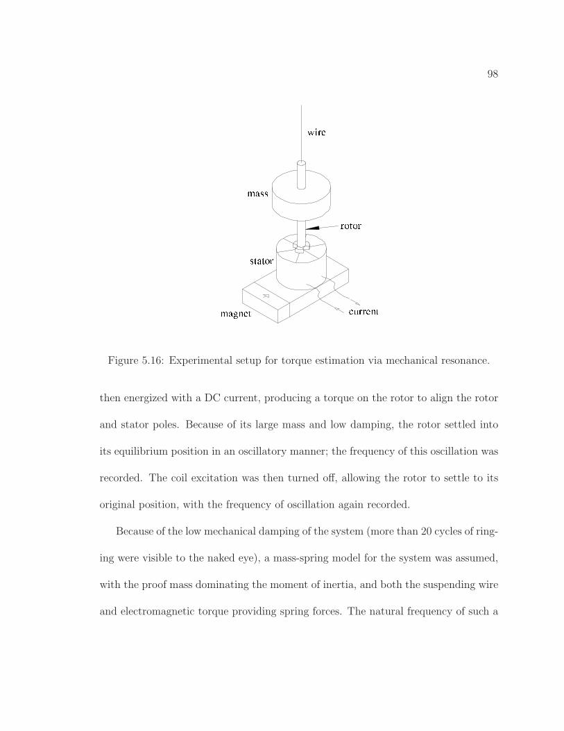
98

Figure 5.16: Experimental setup for torque estimation via mechanical resonance.

then energized with a DC current, producing a torque on the rotor to align the rotor

and stator poles. Because of its large mass and low damping, the rotor settled into

its equilibrium position in an oscillatory manner; the frequency of this oscillation was

recorded. The coil excitation was then turned off, allowing the rotor to settle to its

original position, with the frequency of oscillation again recorded.

Because of the low mechanical damping of the system (more than 20 cycles of ring-

ing were visible to the naked eye), a mass-spring model for the system was assumed,

with the proof mass dominating the moment of inertia, and both the suspending wire

and electromagnetic torque providing spring forces. The natural frequency of such a

99

system is given by

ωn =

√

K

J, (5.9)

where K is the rotational spring constant, and J is the rotational moment of inertia.

For the proof mass, J was calculated to be 24.45×10−9 kg·m2, and oscillation frequen-

cies of 8.55 rad/sec and 15.71 rad/sec were measured for the relaxed and energized

states, respectively. From Eq. 5.9, the calculated spring constants were 1.79×10−6

N·m/rad for the relaxed state, and 6.03×10−6 N·m/rad for the energized state.

The spring constant in the relaxed state is due only to the torsion of the wire,

whereas in the energized state the spring constant comes from both the wire and the

electromagnetic torque. Thus subtracting the two values gives the spring constant

due only to electromagnetic torque, equal to 4.24×10−6 N·m/rad. Assuming peak

torque occurs for the 6 pole generator at π6

rad, the peak torque can be calculated as

2.22×10−6 N·m. The current for this test was 100 mA, and hence the torque constant

for the machine was estimated to be 22.2×10−6 N·m/A. Note that the machine con-

figuration for this experiment was significantly different than that used in later tests,

in that the lower portion of the back iron was removed in order to allow the rotor to

spin freely. Further, due to stretching of the suspension wire, the gap length for the

torque experiment was not well characterized. Thus the torque constant calculated

here differs from the voltage constant calculated in Sec. 5.4.2.

100

5.4.2 Open-Circuit Voltage and Power

The assembled generator was mounted on a test stand that allows axial adjustment

of gap length and lateral adjustment of rotor position. After setting the gap length,

lateral position was manually adjusted for maximum back-emf. As described in Sec.

5.3, permanent magnet excitation was also manually adjusted to maximize back-

emf. Resistance and inductance measurements were then made with an LCR meter

at 120 Hz and 1 kHz. Measured and calculated values for the winding resistance

(Rw), winding inductance (Lw), back-emf constant (Kv), open-circuit voltage (Vo)

and maximum power output (Pout,max) are summarized in Table 5.1.

The nominal speed of operation for the MEMS Wankel engine is a shaft speed of

40 kRPM, corresponding to a rotor speed of 13.3 kRPM, and an electrical frequency

of 667 Hz. All the voltage and power measurements reported here were obtained

by spinning the steel test rotor with an external DC electric motor at 13.3 kRPM.

Because the motor was operated without speed control, variation in the electrical

frequency of about 2.5% was observed. In the following, the actual frequency of

measurements has been noted where appropriate.

Experimental data showing the open-circuit voltage waveform across the generator

terminals appears in Fig. 5.17. The output has a magnitude of approximately 2.63

V at 677 Hz. The subharmonic content is believed to be due to asymmetries in the

rotor which cause variations in the waveform once per shaft rotation, or every three

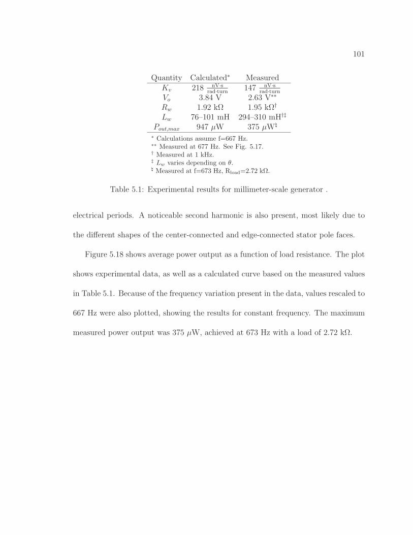
101

Quantity Calculated∗ MeasuredKv 218 nV·s

rad·turn147 nV·s

rad·turn

Vo 3.84 V 2.63 V∗∗

Rw 1.92 k٠1.95 kن

Lw 76–101 mH 294–310 mH†‡

Pout,max 947 µW 375 µW

∗ Calculations assume f=667 Hz.∗∗ Measured at 677 Hz. See Fig. 5.17.† Measured at 1 kHz.‡

Lw varies depending on θ. Measured at f=673 Hz, Rload=2.72 kΩ.

Table 5.1: Experimental results for millimeter-scale generator .

electrical periods. A noticeable second harmonic is also present, most likely due to

the different shapes of the center-connected and edge-connected stator pole faces.

Figure 5.18 shows average power output as a function of load resistance. The plot

shows experimental data, as well as a calculated curve based on the measured values

in Table 5.1. Because of the frequency variation present in the data, values rescaled to

667 Hz were also plotted, showing the results for constant frequency. The maximum

measured power output was 375 µW, achieved at 673 Hz with a load of 2.72 kΩ.

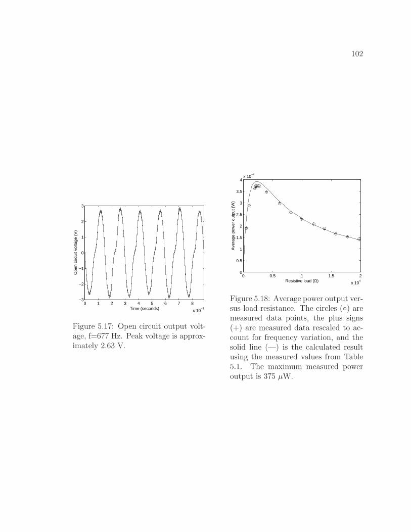
102

0 1 2 3 4 5 6 7 8

x 10−3

−3

−2

−1

0

1

2

3

Time (seconds)

Ope

n ci

rcui

t vol

tage

(V

)

Figure 5.17: Open circuit output volt-age, f=677 Hz. Peak voltage is approx-imately 2.63 V.

0 0.5 1 1.5 2

x 104

0

0.5

1

1.5

2

2.5

3

3.5

4x 10

−4

Resistive load (Ω)

Ave

rage

pow

er o

utpu

t (W

)

Figure 5.18: Average power output ver-sus load resistance. The circles () aremeasured data points, the plus signs(+) are measured data rescaled to ac-count for frequency variation, and thesolid line (—) is the calculated resultusing the measured values from Table5.1. The maximum measured poweroutput is 375 µW.

103

Chapter 6

Machine Design and Analysis —

Centimeter Scale

This chapter extends some of the design ideas of Chapter 5 to the macro scale,

with focus on a power range of tens to hundreds of Watts. As in Chapter 5, the

application of interest is a generator for combustion-based portable power systems,

and hence power density is a key metric. However, it should be noted that there

are an enormous number of applications over a wide range of power levels — from

implantable medical devices to power tools to electric vehicle drives to wind power

generation — that would benefit from high-density motor or generator technology.

The discussion in this chapter pertains to these applications as well, particularly cases

where speed is low, torque is high, and some torque ripple can be tolerated. The first

104

section offers comments on the potential benefits of axial flux machines of the design

under consideration.

6.1 Rationale

There is reason to expect that an axial flux machine having circumferential wind-

ings and a claw-pole stator structure offers the potential for performance improve-

ments over conventional radial flux machines. Enumerated here are several arguments

in favor of such a machine.

• It is generally agreed that axial flux machine configurations achieve higher

torque density than conventional radial-flux machine configurations. The study

in [51], for example, concluded that axial flux machines with radial stator wind-

ings are superior to radial flux designs in terms of power density, moment of

inertia, and iron weight, copper weight, and permanent magnet weight per vol-

ume. Researchers in [53], meanwhile, find that axial flux machines offer higher

specific torque than conventional designs.

One of the main drawbacks of axial flux machines is their poor use of copper.

Because the windings are oriented radially, the copper cross section is limited

by the inner diameter of the winding structure. Using the stator proposed in

Chapter 5 offers the possibility of an air gap geometry that is similar to many

slotted axial flux machine designs, but has dramatically improved winding area.

105

• The back-emf of an electric machine can be increased by increasing its pole

number while holding flux density and speed constant. Total flux linkage per

phase remains the same, while the higher pole number translates to a higher

electrical frequency, and hence a proportionally higher rate of change of flux

linkage and back-emf. However, dividing a conventionally wound stator into

a larger number of poles requires reducing the available winding area propor-

tionally with pole number, as well as increasing winding length proportionally.

Thus winding resistance increases as the square of the pole number. Consider a

rough estimate for the power capability of the machine, taken to be the power

delivered to a resistive load matched to the winding resistance, at speeds where

winding impedance is primarily resistive:

P =V 2

bemf

4R. (6.1)

It is clear that because back-emf voltage increases with pole number, and wind-

ing resistance increases as the square of the pole number, power remains con-

stant over pole number.

Note that the circumferential current configuration, in common with transverse

flux machines, has constant winding resistance as pole number changes. Thus

over some range of pole numbers, power output should scale linearly with pole

number. Of course at higher pole numbers core loss and loss in drive electronics

increase to unacceptable levels, small pole pitch relative to gap length reduces

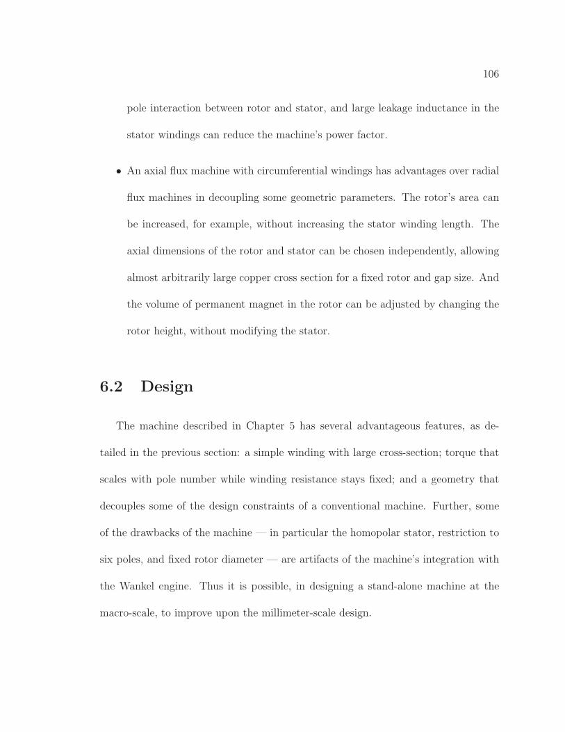
106

pole interaction between rotor and stator, and large leakage inductance in the

stator windings can reduce the machine’s power factor.

• An axial flux machine with circumferential windings has advantages over radial

flux machines in decoupling some geometric parameters. The rotor’s area can

be increased, for example, without increasing the stator winding length. The

axial dimensions of the rotor and stator can be chosen independently, allowing

almost arbitrarily large copper cross section for a fixed rotor and gap size. And

the volume of permanent magnet in the rotor can be adjusted by changing the

rotor height, without modifying the stator.

6.2 Design

The machine described in Chapter 5 has several advantageous features, as de-

tailed in the previous section: a simple winding with large cross-section; torque that

scales with pole number while winding resistance stays fixed; and a geometry that

decouples some of the design constraints of a conventional machine. Further, some

of the drawbacks of the machine — in particular the homopolar stator, restriction to

six poles, and fixed rotor diameter — are artifacts of the machine’s integration with

the Wankel engine. Thus it is possible, in designing a stand-alone machine at the

macro-scale, to improve upon the millimeter-scale design.

107

Figure 6.1: Macro-scale generator design concept.

Figure 6.1 shows a conceptual view of a possible macro-scale design. The combi-

nation of a fixed permanent magnet in the stator and soft magnetic poles in the rotor

has been replaced by a permanent magnet rotor. This allows for reversing rather than

homopolar flux in the stator structure, increasing the magnitude of AC flux linking

the winding by at least a factor of two, and eliminating the sensitivity of the output

to the permanent magnet excitation level. A second phase has also been added by

duplicating the stator structure on the other side of the rotor, with a rotation of

90 electrical degrees (i.e. one half pole pitch). In addition to increasing the power

output, adding a second phase provides smoother torque than a single-phase design,

allows control of rotation direction in motoring operation, and reduces the net axial

forces experienced by the rotor. And finally, a shaft is necessary as the rotor is no

longer supported by the housing as it was at the smaller scale.

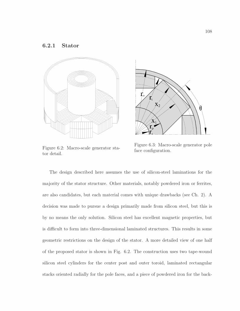
108

6.2.1 Stator

Figure 6.2: Macro-scale generator sta-tor detail.

Figure 6.3: Macro-scale generator poleface configuration.

The design described here assumes the use of silicon-steel laminations for the

majority of the stator structure. Other materials, notably powdered iron or ferrites,

are also candidates, but each material comes with unique drawbacks (see Ch. 2). A

decision was made to pursue a design primarily made from silicon steel, but this is

by no means the only solution. Silicon steel has excellent magnetic properties, but

is difficult to form into three-dimensional laminated structures. This results in some

geometric restrictions on the design of the stator. A more detailed view of one half

of the proposed stator is shown in Fig. 6.2. The construction uses two tape-wound

silicon steel cylinders for the center post and outer toroid, laminated rectangular

stacks oriented radially for the pole faces, and a piece of powdered iron for the back-

109

iron. The stator pole faces presented to the gap are rectangular, with wedge-shaped

slots between them; hence the slot width varies with radius. Furthermore, the poles

are only interdigitated over a fraction of their length, such that the active area (range

of radius shared by all pole faces) is limited. Figure 6.3 shows the stator pole faces

and their related dimensions. Equations 6.2-6.4 give the relations between the pole

face dimensions.

θ = 2πP

(6.2)

x1 = 2rp cos(

θ2

)

(6.3)

x2 = (r2t − r2

p sin2(θ))1

2 (6.4)

A significant change to the stator from the design in Ch. 5 is the introduction of

an axially oriented through-hole for the rotor shaft. This hole runs the length of the

stator center post, using area that would otherwise have been devoted to carrying

magnetic flux. Thus the outer diameter of the center post (and hence the inner

diameter of the winding) must increase somewhat.

6.2.2 Rotor

There are three main possibilities for the configuration of a permanent magnet

rotor: surface magnets; embedded magnets; and the Halbach array. (Some minor

variations on the first two can be found in [75].) A surface magnet rotor for an

axial flux machine is shown in Fig. 6.4. The structure is shown as a linear actuator,

110

but it can be considered as a circumferential slice of the machine in Fig. 6.1. The

magnets are oriented in the axial direction, with alternating polarity. Note that this

configuration requires no soft magnetic material in the rotor. Figure 6.5 shows an

embedded magnet design. The magnets are oriented with alternating polarity in

the circumferential direction, with soft magnetic pieces interposed to direct the flux

axially. Because the cross-sectional area of the magnets can be large compared to the

pole face area that the soft magnetic section presents to the gap, this is sometimes

called a “flux-concentrating” design. This structure can improve the performance of

low energy product magnets by utilizing a greater magnet area. The Halbach array

[78] orients a series of magnets such that flux cancels on one side of the array, and adds

on the other. For large numbers of segments per pole, with magnetization vectors

varying in orientation accordingly, the flux pattern on the additive side approaches

sinusoidal. Because of the one-sided nature of the field, two back-to-back arrays would

be used for a two-phase generator design, as shown in Fig. 6.6.

To compare the fields produced by these three configurations, a two-dimensional

finite-element analysis was performed for each using a generic slotless stator. For

the surface and embedded magnet rotors, the proportion of the rotor occupied by

permanent magnet was varied, while for the Halbach design magnet dimensions are

fixed. The flux density in the middle of the gap for these geometries is plotted for

each design in Figs. 6.7-6.9.

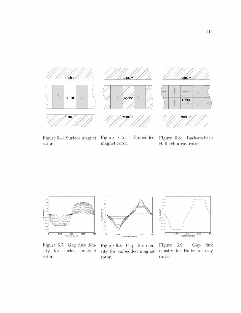
111

Figure 6.4: Surface magnetrotor.

Figure 6.5: Embeddedmagnet rotor.

Figure 6.6: Back-to-backHalbach array rotor.

0 0.005 0.01 0.015 0.02

−0.5

−0.4

−0.3

−0.2

−0.1

0

0.1

0.2

0.3

0.4

0.5

Position in gap (m)

Flu

x de

nsity

(T

)

Figure 6.7: Gap flux den-sity for surface magnetrotor.

0 0.005 0.01 0.015 0.02−1

−0.8

−0.6

−0.4

−0.2

0

0.2

0.4

0.6

0.8

1

Position in gap (m)

Flu

x de

nsity

(T

)

Figure 6.8: Gap flux den-sity for embedded magnetrotor.

0 0.005 0.01 0.015 0.02

−0.5

−0.4

−0.3

−0.2

−0.1

0

0.1

0.2

0.3

0.4

0.5

Position in gap (m)

Flu

x de

nsity

(T

)

Figure 6.9: Gap fluxdensity for Halbach arrayrotor.

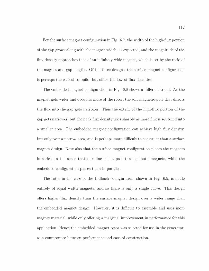
112

For the surface magnet configuration in Fig. 6.7, the width of the high-flux portion

of the gap grows along with the magnet width, as expected, and the magnitude of the

flux density approaches that of an infinitely wide magnet, which is set by the ratio of

the magnet and gap lengths. Of the three designs, the surface magnet configuration

is perhaps the easiest to build, but offers the lowest flux densities.

The embedded magnet configuration in Fig. 6.8 shows a different trend. As the

magnet gets wider and occupies more of the rotor, the soft magnetic pole that directs

the flux into the gap gets narrower. Thus the extent of the high-flux portion of the

gap gets narrower, but the peak flux density rises sharply as more flux is squeezed into

a smaller area. The embedded magnet configuration can achieve high flux density,

but only over a narrow area, and is perhaps more difficult to construct than a surface

magnet design. Note also that the surface magnet configuration places the magnets

in series, in the sense that flux lines must pass through both magnets, while the

embedded configuration places them in parallel.

The rotor in the case of the Halbach configuration, shown in Fig. 6.9, is made

entirely of equal width magnets, and so there is only a single curve. This design

offers higher flux density than the surface magnet design over a wider range than

the embedded magnet design. However, it is difficult to assemble and uses more

magnet material, while only offering a marginal improvement in performance for this

application. Hence the embedded magnet rotor was selected for use in the generator,

as a compromise between performance and ease of construction.

113

6.3 Analysis

This section applies the analysis techniques presented in Chapter 4 to the pro-

posed machine design. The approach is to begin with a lumped-element magnetic

circuit model as in Sec. 4.2, and then apply energy method type analysis to com-

pute torque as in Sec. 4.3. An optimization using Monte Carlo techniques is used to

choose machine dimensions. Finite-element analysis is also applied as in Sec. 4.4 as

a verification of the magnetic circuit analysis.

6.3.1 Lumped-Element Model

The magnetic structure that forms the basis of the lumped element modeling

is shown in Fig. 6.10. Note that although the figure has been “unwrapped” to a

linear rather than rotational actuator as well as “flattened” to a 2-D structure, it

is unchanged magnetically from a qualitative standpoint. The equivalent magnetic

circuit is shown in Fig. 6.11. Reluctances R1 through R8 represent the air gap

between various rotor and stator poles, Ry models the leakage path between adjacent

stator teeth, and Rz models soft magnetic reluctances in the stator. The permanent

magnet is modeled by an MMF source ipm and series reluctance Rv. Because of the

periodic nature of the structure, the two permanent magnets and four windings shown

in Fig. 6.10 can be represented in Fig. 6.11 by a single permanent magnet source

and one winding for each phase. Thus the circuit applies for any number of pole pairs

provided the component values are scaled appropriately.

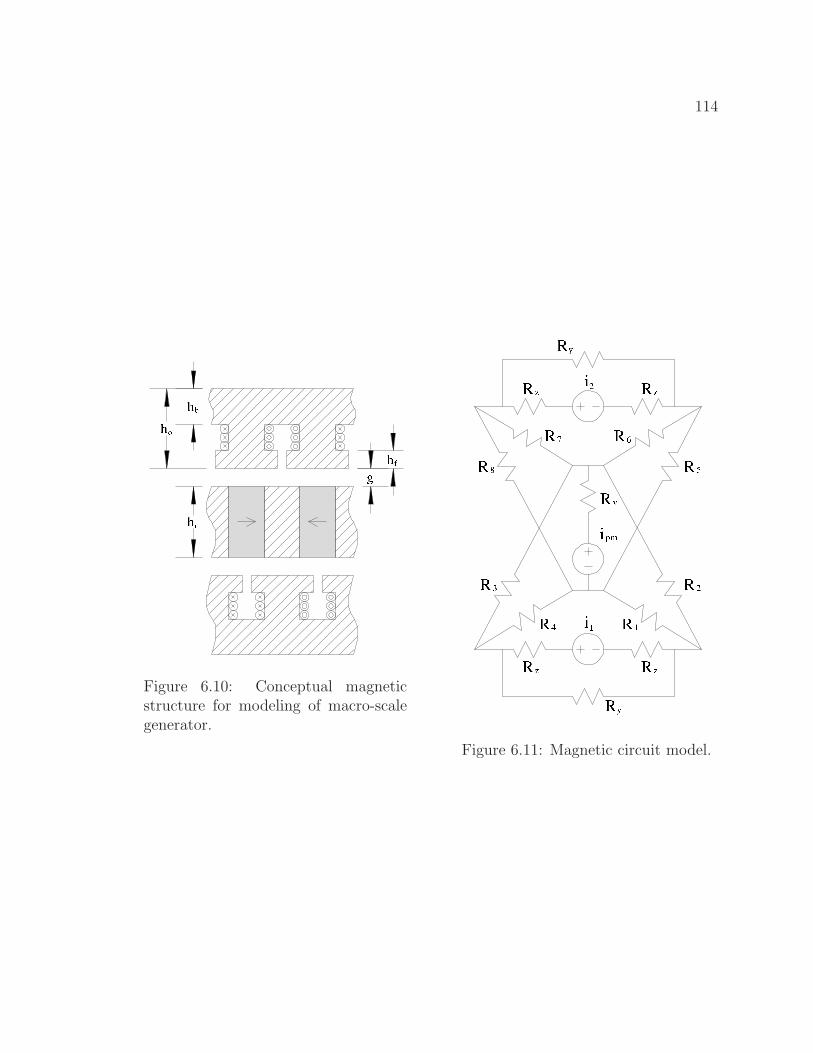
114

Figure 6.10: Conceptual magneticstructure for modeling of macro-scalegenerator.

Figure 6.11: Magnetic circuit model.

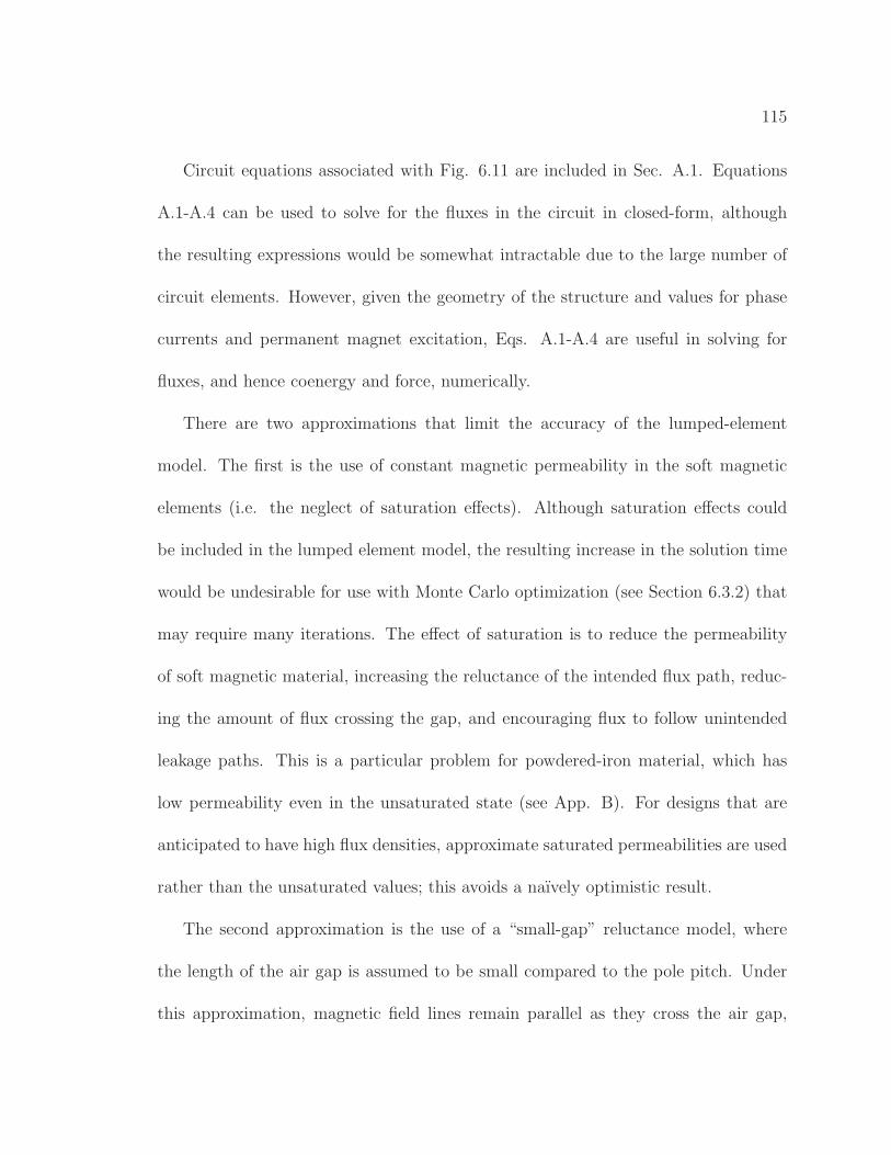
115

Circuit equations associated with Fig. 6.11 are included in Sec. A.1. Equations

A.1-A.4 can be used to solve for the fluxes in the circuit in closed-form, although

the resulting expressions would be somewhat intractable due to the large number of

circuit elements. However, given the geometry of the structure and values for phase

currents and permanent magnet excitation, Eqs. A.1-A.4 are useful in solving for

fluxes, and hence coenergy and force, numerically.

There are two approximations that limit the accuracy of the lumped-element

model. The first is the use of constant magnetic permeability in the soft magnetic

elements (i.e. the neglect of saturation effects). Although saturation effects could

be included in the lumped element model, the resulting increase in the solution time

would be undesirable for use with Monte Carlo optimization (see Section 6.3.2) that

may require many iterations. The effect of saturation is to reduce the permeability

of soft magnetic material, increasing the reluctance of the intended flux path, reduc-

ing the amount of flux crossing the gap, and encouraging flux to follow unintended

leakage paths. This is a particular problem for powdered-iron material, which has

low permeability even in the unsaturated state (see App. B). For designs that are

anticipated to have high flux densities, approximate saturated permeabilities are used

rather than the unsaturated values; this avoids a naıvely optimistic result.

The second approximation is the use of a “small-gap” reluctance model, where

the length of the air gap is assumed to be small compared to the pole pitch. Under

this approximation, magnetic field lines remain parallel as they cross the air gap,

116

and the gap reluctance is well characterized by the gap length and area. However,

for high numbers of poles, pole pitch begins to approach gap length, and the lumped

element model above ceases to be a good approximation. The accuracy of the lumped-

element model could be improved through the use of two-dimensional approximation

techniques such as those found in in [79] or [80], although the added complexity is

perhaps not worth the effort except for extremely simple magnetic structures.

6.3.2 Monte Carlo Optimization

A Monte Carlo method similar to the approach in [81, 82] was used to generate

a set of optimal designs for the lumped element model of Section 6.3.1. Under this

method, six design parameters are randomly chosen from a prespecified range: pole

number; overall radius; center post radius; pole face height; back-iron height; and

winding current. Overall volume, rotor height, shaft radius, and gap height are

held constant. These values are given in Tab. 6.1. The code then computes fluxes

and torque from the magnetic circuit model, and checks that the result is feasible

(i.e. does not have nonphysical dimensions and does not exceed saturation limits).

If a particular design is not feasible, it is discarded and another iteration begins.

Mechanical power is then estimated by taking the peak of the fundamental component

of the torque versus angular displacement curve, and multiplying by the mechanical

frequency in radians per second:

Pmech = max(|τ1|)ωmech. (6.5)

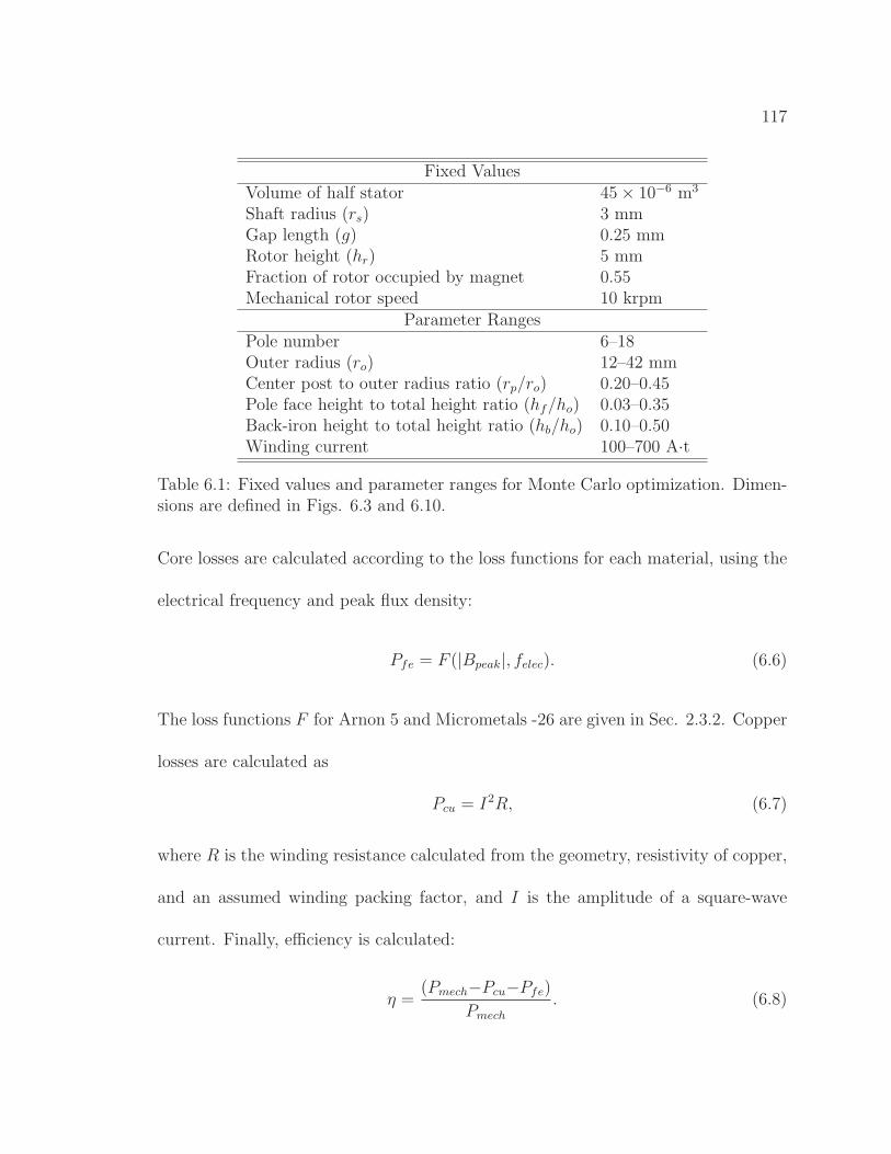
117

Fixed ValuesVolume of half stator 45 × 10−6 m3

Shaft radius (rs) 3 mmGap length (g) 0.25 mmRotor height (hr) 5 mmFraction of rotor occupied by magnet 0.55Mechanical rotor speed 10 krpm

Parameter RangesPole number 6–18Outer radius (ro) 12–42 mmCenter post to outer radius ratio (rp/ro) 0.20–0.45Pole face height to total height ratio (hf/ho) 0.03–0.35Back-iron height to total height ratio (hb/ho) 0.10–0.50Winding current 100–700 A·t

Table 6.1: Fixed values and parameter ranges for Monte Carlo optimization. Dimen-sions are defined in Figs. 6.3 and 6.10.

Core losses are calculated according to the loss functions for each material, using the

electrical frequency and peak flux density:

Pfe = F (|Bpeak|, felec). (6.6)

The loss functions F for Arnon 5 and Micrometals -26 are given in Sec. 2.3.2. Copper

losses are calculated as

Pcu = I2R, (6.7)

where R is the winding resistance calculated from the geometry, resistivity of copper,

and an assumed winding packing factor, and I is the amplitude of a square-wave

current. Finally, efficiency is calculated:

η =(Pmech−Pcu−Pfe)

Pmech

. (6.8)

118

Assuming a design has met the feasibility criteria, its power output and efficiency

are compared with a list of existing “good” designs that have been saved from previous

iterations. If the new design is worse than any individual existing design along both

the power output and efficiency axes, it is discarded. If the new design is superior to

all other designs along at least one of the two axes, it is saved. If the new design is

saved, any existing designs that are worse than the new design along both axes are

discarded.

In this way, over many iterations, a list of quasi-optimal designs is generated which

gives a near-maximum efficiency over a range of power output values, or equivalently

a near-maximum power output over a range of efficiency values. Figure 6.12 shows

a plot of the designs generated using the values in Tab. 6.1. Because the process is

random, designs are not truly optimal — there is a possibility that a design in the list

may be rendered obsolete by a future iteration. However with a sufficient number of

iterations the list can approach the truly optimum curve arbitrarily closely. Note that

not all the points in Fig. 6.12 represent practical continuous operating points. At high

power levels, the machine’s continuous operation may be limited by the dissipation of

heat generated by iron and copper loss. The points in the figure indicated by circles

are acceptable continuous operating points from a thermal point of view, having a

loss to surface area ratio of less than 3000 W/m2. A MATLAB script that performs

the optimization described above is included in Section C.2.

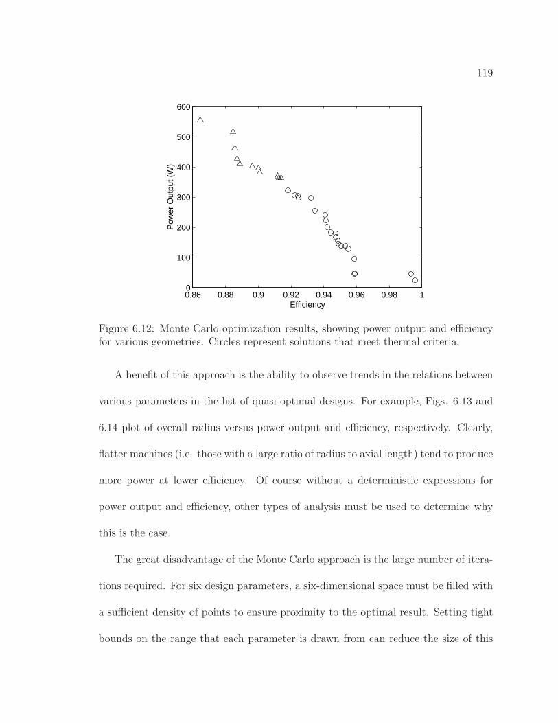
119

0.86 0.88 0.9 0.92 0.94 0.96 0.98 10

100

200

300

400

500

600

Efficiency

Pow

er O

utpu

t (W

)

Figure 6.12: Monte Carlo optimization results, showing power output and efficiencyfor various geometries. Circles represent solutions that meet thermal criteria.

A benefit of this approach is the ability to observe trends in the relations between

various parameters in the list of quasi-optimal designs. For example, Figs. 6.13 and

6.14 plot of overall radius versus power output and efficiency, respectively. Clearly,

flatter machines (i.e. those with a large ratio of radius to axial length) tend to produce

more power at lower efficiency. Of course without a deterministic expressions for

power output and efficiency, other types of analysis must be used to determine why

this is the case.

The great disadvantage of the Monte Carlo approach is the large number of itera-

tions required. For six design parameters, a six-dimensional space must be filled with

a sufficient density of points to ensure proximity to the optimal result. Setting tight

bounds on the range that each parameter is drawn from can reduce the size of this

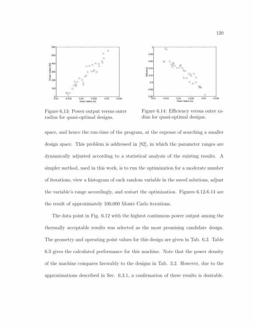
120

0.01 0.015 0.02 0.025 0.03 0.0350

100

200

300

400

500

600

Outer radius (m)

Pow

er o

utpu

t (W

)

Figure 6.13: Power output versus outerradius for quasi-optimal designs.

0.01 0.015 0.02 0.025 0.03 0.0350.86

0.88

0.9

0.92

0.94

0.96

0.98

1

Outer radius (m)

Effi

cien

cy

Figure 6.14: Efficiency versus outer ra-dius for quasi-optimal designs.

space, and hence the run-time of the program, at the expense of searching a smaller

design space. This problem is addressed in [82], in which the parameter ranges are

dynamically adjusted according to a statistical analysis of the existing results. A

simpler method, used in this work, is to run the optimization for a moderate number

of iterations, view a histogram of each random variable in the saved solutions, adjust

the variable’s range accordingly, and restart the optimization. Figures 6.12-6.14 are

the result of approximately 100,000 Monte Carlo iterations.

The data point in Fig. 6.12 with the highest continuous power output among the

thermally acceptable results was selected as the most promising candidate design.

The geometry and operating point values for this design are given in Tab. 6.2. Table

6.3 gives the calculated performance for this machine. Note that the power density

of the machine compares favorably to the designs in Tab. 3.2. However, due to the

approximations described in Sec. 6.3.1, a confirmation of these results is desirable.

121

P 10ro 25.1 mmrp 9.8 mmhf 4.0 mmhb 7.7 mmIw 405 A·t

Table 6.2: Design values chosen fromMonte Carlo optimization results.

Pout 323 WPcu 7.7 WPcore 21.1 Wη 0.92P ′ 3.2 × 106 W/m3

Table 6.3: Machine performance calcu-lated from magnetic circuit results.

Finite-element analysis can be employed for this purpose, as described in the next

section.

6.3.3 Finite-Element Analysis

Finite-element analysis, as described in Sec. 4.4, was applied to the two-dimensional

model shown in Fig. 6.15, which is qualitatively equivalent to Fig. 6.10. As in Fig.

6.10, this structure represents two poles of a circumferential cross-section of the ma-

chine taken at a particular radius. The commercial finite-element software package

FEMLAB was used to obtain the solution.

As compared to lumped-element analysis, finite-element analysis captures more

closely the effects of realistic field geometries. Further, the soft magnetic portions of

the model include the saturation effects described in Sec. 2.1. This is accomplished

by defining the magnetic permeability of these regions of the model with a saturating

function of flux density, given by

µr(B) =µr

C|B|2 + 1+ 1. (6.9)

122

For silicon steel µr=1000, while for powdered iron material µr=75; for both materials,

C=25. (Information on magnetic material properties can be found in App. B.)

The use of nonlinear materials complicates somewhat the calculation of coenergy

density within the material. Rather than a linear calculation based only on the (B,H)

operating point, the integral of Eq. 4.38 must be carried out over the particular B,H

trajectory taken to reach the operating point. Equation 6.9 defines this trajectory —

details of how the integration is carried out can be found in Sec. A.3.

A two-dimensional finite-element model was selected due to the extreme compu-

tational requirements a three-dimensional model would impose. The machine under

consideration, however, has features that are not uniform in the radial direction. For

example, a true circumferential cross-section of the machine at the radii of interest

has no pole teeth — only pole faces appear, because the vertical pole tooth structure

is confined to the radii of the center post and toroid. Magnetically, however, there

must be a low-permeability path in the two-dimensional model that allows the flux to

link the winding. This is handled by inserting a vertical member that has the same

reluctance as the true three dimensional path.

Consider a reluctance Ro = ℓo

µoµrAo, in which ℓo and Ao reflect the actual dimensions

of the machine, and µr the actual material’s relative permeability. Then suppose that

for the purposes of modeling the area must be scaled by a factor 0 < S < 1. Clearly,

to achieve the same reluctance, the permeability can be scaled by 1S. The length

could also be scaled, but it is desirable to maintain as much as possible of the original

123

geometry. For nonlinear materials, a further issue arises. Assume the reduced-area

model reluctance is to carry the same flux as its real-world counterpart. Because it

has a smaller area, its flux density will be higher, with the result that permeability

will begin to decrease earlier than it should. Hence the flux density must also be

corrected, by scaling B by a factor S. A rescaled version of Eq. 6.9, for a model with

area scaled by S, is thus

µr(B) =1

S

(

µr

C|SB|2 + 1+ 1

)

. (6.10)

Another three-dimensional feature of the geometry is the slot between stator poles.

As can be seen from Fig. 6.3, the width of the slot is a function of radius. To account

for this variation, a full torque versus displacement curve was calculated at each of

three different radii. A second-order polynomial was then fit to the results in the

radial direction, and integration carried out to attempt to capture more accurately

the torque over the useful range of radii. Details of this procedure can be found in

Sec. A.2.

A 2-D finite-element model was created for the candidate design, using the dimen-

sions and current in Tab. 6.2. Square wave currents were assumed, with all windings

carrying the same magnitude current. Figure 6.16 shows the FEA solution for the dis-

placement where the rotor is aligned with the stator. Qualitatively it is apparent from

the figure how the field differs from the lumped-element “small-gap” approximation.

A more quantitative comparison is given by Fig. 6.17, in which the flux linkage of one

phase winding is shown for both the lumped-element and finite-element models. The

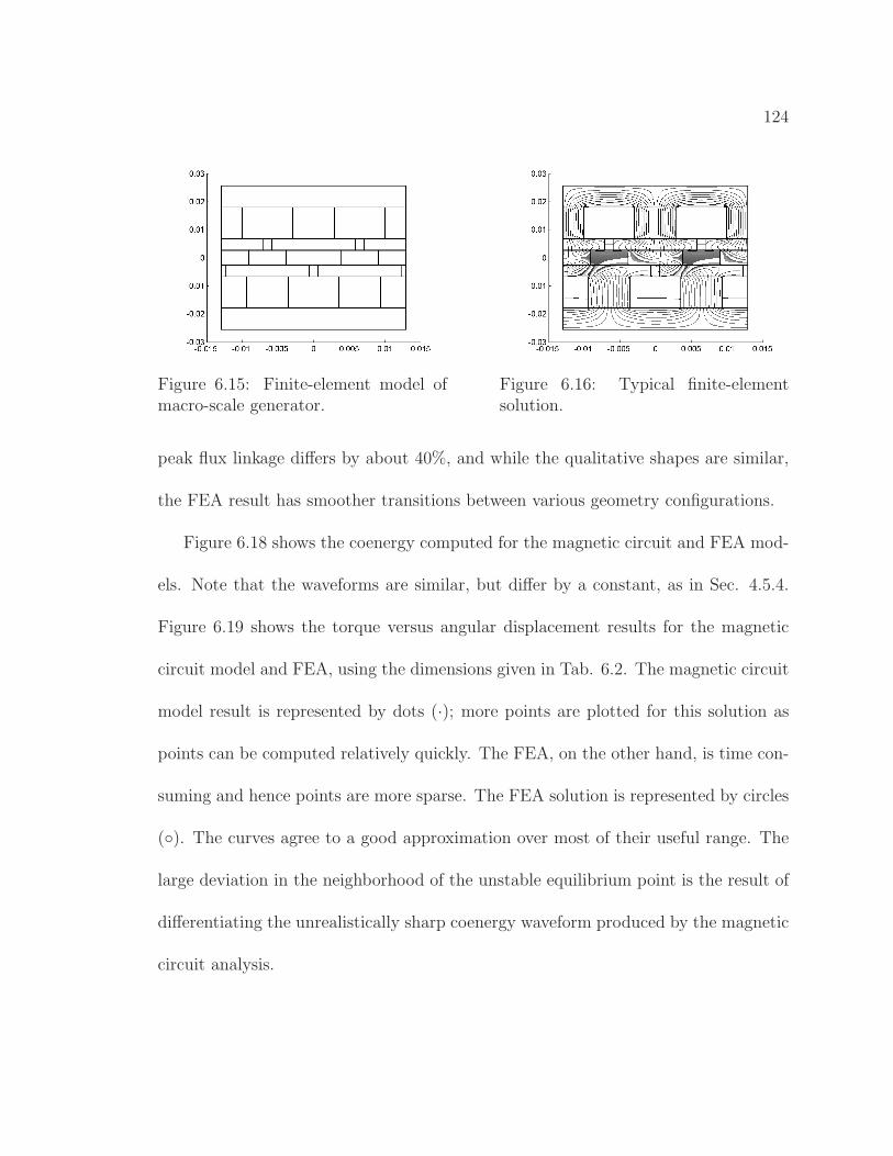
124

Figure 6.15: Finite-element model ofmacro-scale generator.

Figure 6.16: Typical finite-elementsolution.

peak flux linkage differs by about 40%, and while the qualitative shapes are similar,

the FEA result has smoother transitions between various geometry configurations.

Figure 6.18 shows the coenergy computed for the magnetic circuit and FEA mod-

els. Note that the waveforms are similar, but differ by a constant, as in Sec. 4.5.4.

Figure 6.19 shows the torque versus angular displacement results for the magnetic

circuit model and FEA, using the dimensions given in Tab. 6.2. The magnetic circuit

model result is represented by dots (·); more points are plotted for this solution as

points can be computed relatively quickly. The FEA, on the other hand, is time con-

suming and hence points are more sparse. The FEA solution is represented by circles

(). The curves agree to a good approximation over most of their useful range. The

large deviation in the neighborhood of the unstable equilibrium point is the result of

differentiating the unrealistically sharp coenergy waveform produced by the magnetic

circuit analysis.

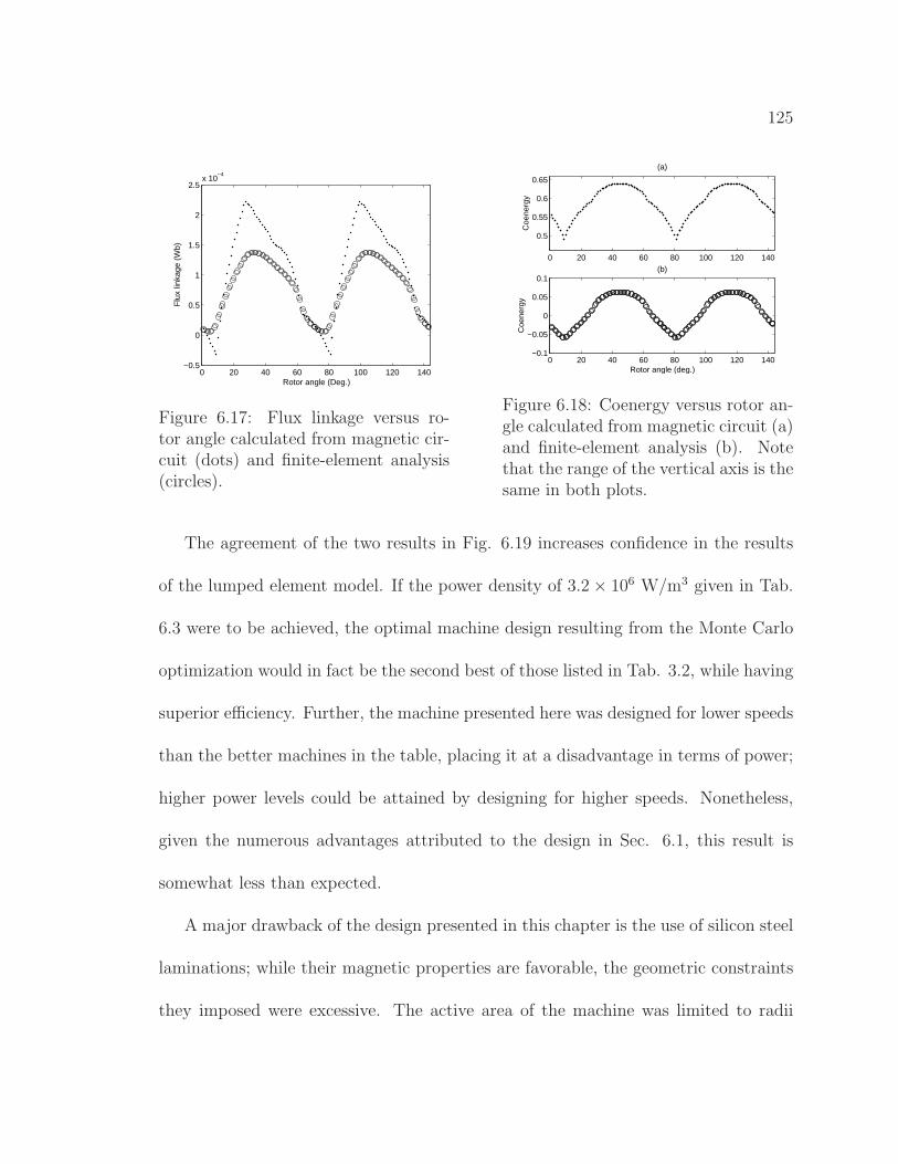
125

0 20 40 60 80 100 120 140−0.5

0

0.5

1

1.5

2

2.5x 10

−4

Rotor angle (Deg.)

Flu

x lin

kage

(W

b)

Figure 6.17: Flux linkage versus ro-tor angle calculated from magnetic cir-cuit (dots) and finite-element analysis(circles).

0 20 40 60 80 100 120 140

0.5

0.55

0.6

0.65

Coe

nerg

y

(a)

0 20 40 60 80 100 120 140−0.1

−0.05

0

0.05

0.1

Coe

nerg

y

Rotor angle (deg.)

(b)

Figure 6.18: Coenergy versus rotor an-gle calculated from magnetic circuit (a)and finite-element analysis (b). Notethat the range of the vertical axis is thesame in both plots.

The agreement of the two results in Fig. 6.19 increases confidence in the results

of the lumped element model. If the power density of 3.2 × 106 W/m3 given in Tab.

6.3 were to be achieved, the optimal machine design resulting from the Monte Carlo

optimization would in fact be the second best of those listed in Tab. 3.2, while having

superior efficiency. Further, the machine presented here was designed for lower speeds

than the better machines in the table, placing it at a disadvantage in terms of power;

higher power levels could be attained by designing for higher speeds. Nonetheless,

given the numerous advantages attributed to the design in Sec. 6.1, this result is

somewhat less than expected.

A major drawback of the design presented in this chapter is the use of silicon steel

laminations; while their magnetic properties are favorable, the geometric constraints

they imposed were excessive. The active area of the machine was limited to radii

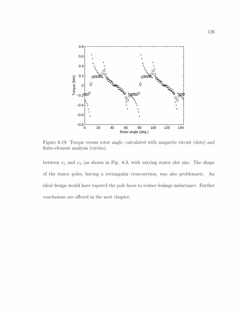
126

0 20 40 60 80 100 120 140−0.8

−0.6

−0.4

−0.2

0

0.2

0.4

0.6

0.8

Rotor angle (deg.)

Tor

que

(Nm

)

Figure 6.19: Torque versus rotor angle, calculated with magnetic circuit (dots) andfinite-element analysis (circles).

between x1 and x2 (as shown in Fig. 6.3, with varying stator slot size. The shape

of the stator poles, having a rectangular cross-section, was also problematic. An

ideal design would have tapered the pole faces to reduce leakage inductance. Further

conclusions are offered in the next chapter.

127

Chapter 7

Conclusions

Efficient and dense electromechanical energy conversion is a key component of

many proposed portable power systems. Further, applications for such systems are

numerous and growing. Two designs were presented for generators having axial flux

and circumferential windings. Although their size and application requirements dif-

fer somewhat, the two machines have many common elements. This chapter offers

reflections and conclusions drawn from these two design efforts, as well as an outline

for future research.

7.1 Thoughts on Millimeter-Scale Design

Because the millimeter-scale design was intended to interact with a planar MEMS

internal combustion engine, many design choices were guided by the engine configura-

tion. The integrated design of the engine and generator, while novel, was a limitation

128

on both devices. A permanent magnet rotor would have been the most appropriate

choice, but temperature constraints made this impractical. The simpler option of

soft magnetic poles nonetheless complicated the silicon rotor fabrication, while the

size and shape of the rotor constrained the soft magnetic material to a sub-optimal

configuration.

Although the two devices were never tested together, there was a potential mis-

match in sizing between the engine and generator in terms of power output. Inte-

gration again constrained the two designs, such that the calculated maximum input

power of the generator was less than the calculated output power of the engine [26].

Interestingly, the generator power ideally increases as the fourth power of a uniform

scaling factor (see Eq. 3.10), while the engine scales as the third power; in theory

there is an appropriate size where an integrated engine-generator design matches the

power of the two machines.

The homopolar flux configuration of the stator introduced two problems. The first

was large flux leakage in the non-aligned rotor position, which reduced the magnitude

of the AC flux linking the stator winding. The second was stator saturation, which

was experimentally demonstrated to reduce the power output of the machine. Thus

great care must be taken to find the optimal flux level. A design with a permanent

magnet rotor, such as in Ch. 6, has fully reversing flux, and hence should be able to

increase the AC flux linkage by at least of factor of two.

129

Machining of powdered iron proved to be problematic. The materials tested were

brittle and inhomogenous, resulting in frequent fractures when machining small parts.

Sharp tools, high cutting speeds, and sacrificial supporting jigs mitigate this problem

somewhat, but it may be preferable to have parts pressed from molds.

The powdered iron also proved to be undesirable magnetically. The low perme-

ability of the material required that key portions of the stator (i.e. the center post

and toroid, which carry the highest flux densities) be made from silicon steel.

7.2 Thoughts on Centimeter-Scale Design

The design process described in Chapter 6 is iterative, because none of the analyses

available are appropriate for the entire problem. Magnetic circuit techniques are fast

but make substantial approximations, while finite-element techniques can be more

accurate but are often too slow for use in optimization problems that require many

solution iterations. Thus the approach was to develop a first-pass optimal design

with magnetic circuit techniques, and use FEA to verify its performance and fine-

tune calculations.

The resulting machine is calculated to have 323 W maximum continuous power

output at just under 92% efficiency, with a power density of 3.2 × 106 W/m3. This

places the design among some of the better machines in Table 3.2. The design speed

was relatively low, indicating that further gains could be realized by designing for

130

higher speeds. On the other hand, the calculated performance, particularly core loss,

may prove to be optimistic; this can only be verified by experimentation.

An issue that is left unresolved is the true upper bound on the performance of such

a machine. Basic calculations indicate that torque should scale with pole number.

Of course, higher pole numbers demand higher electrical frequencies, and at a certain

point core losses will be excessive. There is also a practical limitation on pole number

imposed by the gap length — when the pole pitch becomes small, flux no longer

crosses the gap. It is not clear from the Monte Carlo result which of these effects is

primarily responsible for limiting the pole number of the optimal designs.

Nontheless, the factors that negatively impact performance are practical, not fun-

damental. Smaller gaps, low loss materials, and careful design to minimize winding

inductance could provide further performance increases. It is also possible that some

of the design ideas presented here could be useful in MEMS applications, where gaps

can be smaller, allowing larger numbers of poles. Microfabrication also offers different

material and fabrication choices, which may resolve the conflict between silicon steel

and powdered iron.

7.3 Thoughts on Future Research Directions

As noted in Chapter 6, the axial-flux circumferential current machine has potential

to improve on the power density of conventional machines. However, as was also

131

shown, obstacles exist that degrade the performance of the design. Suggestions for

future research are presented below.

7.3.1 Isotropic Materials

The use of silicon steel laminations for the design in Chapter 6, while providing

for good magnetic properties, may have introduced excessive limitations on geometry.

A larger effective stator pole area, for example, might be obtained through the use

of an isotropic material. Such a material would also allow the leakage between stator

poles to be minimized by tapering and otherwise shaping the poles. Indeed, with

isotropic materials, the design space becomes much larger, and more opportunities

arise for improved performance.

However, a larger design space also implies greater difficulty in finding an optimum

design. Further, available isotropic materials have poor magnetic properties. Thus

the greater losses and low permeability of powdered iron materials may offset the

advantages of its isotropic nature. A similar challenge comes from the low saturation

flux density of ferrite material.

7.3.2 Small Gap, Low Speed Machine

If the machine design is freed from the speed constraints of a particular application,

core loss no longer places a limit on pole number — the machine can simply be run

at a speed where core losses are acceptable, including DC if necessary. The design

132

problem is then that of maximizing torque rather than power, and the optimal pole

number and hence maximum torque is determined by the gap length. Hence the

challenge is mainly the mechanical issue of constructing a machine with an extremely

small gap.

The research effort would consist of optimization of the magnetic structure with

gap length as a parameter, such that the relationship between optimal pole number

and gap length is well characterized. This would be followed by careful thermal analy-

sis and mechanical design, perhaps utilizing novel machining and assembly techniques

to meet tight tolerances, or creating novel structures having compliance for thermal

expansion while still maintaining gap spacing.

7.3.3 Materials and Manufacturing

The material options that currently exist for complex three-dimensional magnetic

structures are poor. Isotropic materials such as powdered iron or ferrites carry penal-

ties in magnetic performance, while silicon steel laminations are difficult to form into

the required geometries.

There are several diverse avenues for addressing this problem. A straightforward

approach may be to examine hybrid structures, that make use of multiple types of

material depending on the particular requirements. This was done in both Ch. 5 and

Ch. 6, in which silicon steel was used for high-saturation components while powdered

iron was used in components that required isotropic properties.

133

An alternative approach might be to investigate methods of producing three-

dimensional structures from silicon steel laminations, utilizing complex cut and folded

shapes. Finally, a risky approach to the problem might attempt to produce better

magnetic materials, perhaps via novel electroplating processes. This would require

significant innovation, however, and may not be feasible on a large scale.

134

Bibliography

[1] (2005) Phonescoop. Database of mobile phone information. Phone Factor, LLC.[Online]. Available: http://www.phonescoop.com

[2] (2005) Cellphone battery warehouse. Product Catalog. Cellphone BatteryWarehouse, LLC. [Online]. Available: http://www.batteries4less.com

[3] (2005) Dell. Product Catalog. Dell, Inc. [Online]. Available:http://www.dell.com

[4] (2005) 4allbatteries.com. Product Catalog. 4 All Batteries. [Online]. Available:http://www.4allbatteries.com

[5] “Statistical review – business appliances,” Appliance, Gartner Group, 2004.

[6] J. Haughey, “Is technology adoption quickening?” Electronic Business, Interna-tional Telecom Union, p. 16, Aug. 2004.

[7] Committee on Electric Power for the Dismounted Soldier, “Energy–efficient tech-nologies for the dismounted soldier,” Technical report, National Research Coun-cil, 1997.

[8] P. Flynn et al , “Meeting the energy needs of future warriors,” Technical Report,National Research Council, 2004.

[9] N. Lewis et al , “Portable energy for the dismounted soldier,” Technical Report,The MITRE Corporation, 2003.

[10] A. Patil, “U.S. Army CERDEC fuel cell technology,” presented at Science at theLeading Edge (170th Annual Meeting of the AAAS). American Association forthe Advancement of Science, Feb. 2004.

[11] J. Jansen et al , “Exoskeleton for soldier enhancement systems feasibility study,”Technical report, Oak Ridge National Laboratory, 2000.

[12] J. Grasmeyer and M. Keennon, “Development of the black widow micro air vehi-cle,” presented at the 39th Aerospace Sciences Meeting and Exhibit. AmericanInstitute of Aeronautics and Astronautics, Inc., 2001, paper AIAA-2001-0127.

135

[13] (2004) Epson announces advanced model of the world’s lightest micro-flying robot. Press Release. Seiko Epson Corp. [Online]. Available:http://www.epson.co.jp/e/newsroom/news 2004 08 18.htm

[14] M. Woods, J. Henderson, and G. Lock, “Energy requirements for the flight ofmicro air vehicles,” The Aeronautical Journal, vol. 105, no. 1045, pp. 135–149,March 2001.

[15] J. Hill, M. Horton, R. Kling, and L. Krishnamurthy, “The platforms enablingwireless sensor networks,” Communications of the ACM, vol. 47, no. 6, pp. 41–6,June 2004.

[16] S. Roundy, D. Steingart, L. Frechette, P. Wright, and J. Rabaey, “Power sourcesfor wireless sensor networks,” in Wireless Sensor Networks, First EuropeanWorkshop. Springer-Verlag, 2004, pp. 1–17.

[17] P. Krein, “The power of forever: managing the ultimate in long-term energyneeds of spacecraft and other remote systems,” Power and energy seminar pre-sentation, University of Illinois at Urbana-Champaign, Oct. 2004.

[18] P. Glynne-Jones, M. Tudor, S. Beeby, and N. White, “An electromagnetic,vibration-powered generator for intelligent sensor systems,” Sensors and Acu-tators, A: Physical, vol. 110, no. 1-3, pp. 344–9, Feb. 2004.

[19] S. Roundy, P. Wright, and K. Pister, “Micro-electrostatic vibration-to-electricityconverters,” in 2002 AMSE International Mechanical Engineering Congress andExposition. ASME, Nov. 2002, pp. 487–96.

[20] S. Roundy, P. Wright, and J. Rabaey, “A study of low level vibrations as a powersource for wireless sensor nodes,” Computer Communications, vol. 26, no. 11, pp.1131–44.

[21] T. R. Crompton, Battery Reference Book. Reed Educational and ProfessionalPublishing, 2000.

[22] E. Jonietz, “Ant power packs,” Technology Review, Sept. 2004.

[23] Y. Zhu, S. Ha, and R. Masel, “High power density direct formic acid fuel cells,”Journal of Power Sources, vol. 130, no. 1-2, pp. 8–14, May 2004.

[24] A. C. Fernandez-Pello, “Micropower generation using combustion: issues andapproaches,” in Twenty-ninth International Symposium on Combustion, vol. 29.Proceedings of the Combustion Institute, 2002, pp. 883–98.

136

[25] A. H. Epstein et al , “Power MEMS and microengines,” in 1997 InternationalConference on Solid–State Sensors and Actuators (TRANSDUCERS ’97), vol. 2.IEEE, 1997, pp. 753–6.

[26] A. J. Knobloch, “Ultra–deep reactive ion etching for silicon wankel internal com-bustion engines,” Ph.D. dissertation, University of California, Berkeley, 2003.

[27] A. J. Knobloch, M. Wasilik, C. Fernandez-Pello, and A. P. Pisano, “Microinternal-combustion engine fabrication with 900 µm deep features via DRIE,”in 2003 ASME International Mechanical Engineering Congress, vol. 5. ASME,Nov. 2003, pp. 115–23.

[28] D. G. Jones and A. P. Pisano, “Fabrication of ultra thick ferromagnetic structuresin silicon,” in 2004 ASME International Mechanical Engineering Congress andExposition. ASME, 2004.

[29] F. C. Martinez, “Apex seal design for the MEMS rotary engine power system,”Master’s thesis, University of California, Berkeley, 2000.

[30] B. Haendler, “Liquid to vapor phase change in constant cross-section siliconmicrochannels,” Master’s thesis, University of California, Berkeley, 2003.

[31] R. Boll, ed., Soft Magnetic Materials : Fundamentals, Alloys, Properties, Prod-ucts, Applications. Heyden, 1979.

[32] R. C. O’Handley, Modern Magnetic Materials: Principles and Applications.John Wiley & Sons, Inc., 2000.

[33] R. M. Bozorth, Ferromagnetism. American Telephone and Telegraph Company,1978.

[34] J. F. Gieras and M. Wing, Permanent Magnet Motor Technology. MarcelDekker, Inc., 2002.

[35] E. P. Furlani, Permanent Magnet and Electromechanical Devices. AcademicPress, 2001.

[36] A. E. Fitzgerald, C. Kingsley, Jr., and S. Umans, Electric Machinery. McGraw–Hill, 1990.

[37] (2003) Precision rolled strip & foil. Product catalog. Arnold. [Online]. Available:http://www.arnoldmagnetics.com

[38] (2003) Iron powder cores for power conversion and line filter applications. Prod-uct catalog. Micrometals, Inc. [Online]. Available: http://www.micrometals.com

137

[39] N. Maluf, An Introduction to Microelectromechanical Systems Engineering.Artech House, Inc., 2000.

[40] D. P. Arnold, I. Zana, F. Cros, and M. G. Allen, “Vertically laminated mag-netic cores by electroplating ni-fe into micromachined si,” IEEE Transactions onMagnetics, vol. 40, no. 4, pp. 3060–62, July 2004.

[41] T. Budde, M. Fohse, B. Majjer, H. Luthje, G. Brauer, and H. H. Gatzen, “Aninvestigation on technologies to fabricate magnetic microcomponents for minia-turized actuator systems,” Microsystem Technologies, vol. 11, no. 1, pp. 78–84,February 2002.

[42] W. P. Taylor, M. Schneider, H. Baltes, and M. G. Allen, “A NiFeMo electroplat-ing bath for micromachined structures,” Electrochemical and Solid-State Letters,vol. 2, no. 12, pp. 624–6, December 1999.

[43] N. V. Myung, D.-Y. Park, B.-Y. Yoo, and P. T. A. Sumodjo, “Development ofelectroplated magnetic materials for MEMS,” Journal of Magnetism and Mag-netic Materials, vol. 265, no. 2, pp. 189–98, September 2003.

[44] H. J. Cho and C. H. Ahn, “Microscale resin-bonded permanent magnets formagnetic micro-electro-mechanical systems applications,” Journal of AppliedPhysics, vol. 93, no. 10, pp. 8674–6, May 2003.

[45] L. K. Lagorce, O. Brand, and M. G. Allen, “Magnetic microactuators basedon polymer magnets,” IEEE Journal of Microelectromechanical Systems, vol. 8,no. 1, pp. 2–9, March 1999.

[46] H. J. Cho and C. H. Ahn, “A bidirectional magnetic microactuator using electro-plated permanent magnet arrays,” Journal of Microelectromechanical Systems,vol. 10, no. 3, pp. 237–40, March 2004.

[47] B. Pawlowski, S. Schwarzer, A. Rahmig, and J. Topfer, “NdFeB thick filmsprepared by tape casting,” Journal of Magnetism and Magnetic Materials, vol.265, no. 3, pp. 337–44, October 2003.

[48] T. Budde and H. H. Gatzen, “Magnetic properties of an SmCo/NiFe system formagnetic microactuators,” Journal of Magnetism and Magnetic Materials, vol.272-276, no. 3, pp. 2027–8, May 2004.

[49] J.-C. Shih, H.-H. Hsiao, J.-L. Tsai, and T.-S. Chin, “Low-temperature in-situgrowth of high-coercivity Fe-Pt films,” IEEE Transactions on Magnetics, vol. 37,no. 4, pp. 1280–2, July 2001.

138

[50] S. Franz, P. Cavallotti, M. Bestetti, V. Sirtori, and L. Lombardi, “Electrode-position of cobalt platinum alloys micromagnets,” Journal of Magnetism andMagnetic Materials, vol. 272-276, no. 3, pp. 2430–1, May 2004.

[51] K. Sitapati and R. Krishnan, “Performance comparisons of radial and axial field,permanent-magnet, brushless machines,” IEEE Transactions on Industry Appli-cations, vol. 37, no. 5, pp. 1219–26, Sept./Oct. 2001.

[52] S. Huang, J. Luo, F. Leonardi, and T. A. Lipo, “A comparison of power den-sity for axial flux machines based on general purpose sizing equations,” IEEETransactions on Energy Conversion, vol. 14, no. 2, pp. 185–92, June 1999.

[53] N. B. Simsir and H. B. Ertan, “A comparison of torque capabilities of axialflux and radial flux type of brushless DC (BLDC) drives for wide speed rangeapplications,” in 1999 International Conference on Power Electronics and DriveSystems (PEDS ’99). IEEE, Jul. 1999, pp. 719–24.

[54] W. Arshad, T. Backstrom, and C. Sadarangani, “Analytical design and analysisprocedure for a transverse flux machine,” in International Electric Machines andDrives Conference (IEMDC 2001). IEEE, Jun. 2001, pp. 115–21.

[55] P. L. Chapman and P. T. Krein, “Micromotor technology: Electric drive de-signer’s perspective,” in Conference Record of the 2001 IEEE Industry Applica-tions Society Annual Meeting, vol. 3. IEEE, 2001, pp. 1978–83.

[56] J. W. Judy, “Batch–fabricated ferromagnetic microactuators with silicon flex-ures,” Ph.D. dissertation, University of California, Berkeley, 1996.

[57] (2005) Maxon motors. Product catalog. Maxon Motor A.G. [Online]. Available:http://www.maxonmotor.com

[58] (2005) Faulhaber brushless motors. Product catalog. FAULHABER Group.[Online]. Available: http://www.micromo.com/products

[59] L.-S. Fan, Y.-C. Tai, and R. S. Muller, “IC-processed electrostatic micromotors,”Sensors and Actuators, vol. 20, no. 1-2, pp. 41–7, Nov. 1989.

[60] H. Guckel et al , “Fabrication and testing of the planar magnetic micromotor,”Journal of Micromechanics & Microengineering, vol. 1, no. 3, pp. 135–8, Sept.1991.

[61] ——, “A first functional current excited planar rotational magnetic micromotor,”in Micro Electro Mechanical Systems. IEEE, Feb. 1993, pp. 7–11.

139

[62] T. Christenson, H. Guckel, and J. Klein, “A variable reluctance stepping mi-crodynamometer,” Microsystem Technologies, vol. 2, no. 3, pp. 139–43, Aug.1996.

[63] H. Koser and F. Cros and M. G. Allen and J. H. Lang, “A high torque densityMEMS magnetic induction machine,” in 11th International Conference on Solid–State Sensors and Actuators (TRANSDUCERS ’01), vol. 1. Springer–Verlag,2001, pp. 284–7.

[64] H. Koser and J. H. Lang, “Modeling a high power density MEMS magneticinduction machine,” in 2001 International Conference on Modeling and Simula-tion of Microsystems, vol. 1. Nano Science and Technology Institute, 2001, pp.286–9.

[65] David P. Arnold et al , “Magnetic induction machines embedded in fusion-bondedsilicon,” presented at the Solid-State Sensor, Actuator and Microsystems Work-shop (Hilton Head 2004), 2004.

[66] M. Nienhaus, W. Ehrfeld, H.-D. Stolting, F. Michel, S. Kleen, S. Hardt,F. Schmitz, and T. Stange, “Design and realization of a penny-shaped micromo-tor,” in Design, Test, and Microfabrication of MEMS and MOEMS, vol. 3680.SPIE - the International Society for Optical Engineering, 1999, pp. 592–600.

[67] T. Kohlmeier, V. Seidemann, S. Buttgenbach, and H. H. Gatzen, “Application ofUV depth lithography and 3D-microforming for high aspect ratio electromagneticmicroactuator components,” Microsystem Technologies, vol. 8, no. 4-5, pp. 304–7, Aug. 2002.

[68] J. Edler, H.-D. Stolting, M. Fohse, and H. H. Gatzen, “A linear microactuatorwith enhanced design,” Microsystem Technologies, vol. 7, no. 5-6, pp. 261–4, Jan.2002.

[69] J. R. Melcher, Continuum Electromechanics. MIT Press, 1981.

[70] H. H. Woodson and J. R. Melcher, Electromechnical Dynamics. John Wiley &Sons, Inc., 1968.

[71] J.-M. Jin, The Finite Element Method in Electromagnetics. John Wiley & Sons,Inc., 2002.

[72] J. Luo, D. Qin, T. A. Lipo, S. Li, and S. Huang, “Axial flux circumferential cur-rent permanent magnet (AFCC) machine,” in 1998 IEEE Industry ApplicationsConference, vol. 1. IEEE, 1998, pp. 144–51.

140

[73] J. Cros, J. R. Figueroa, and P. Viarouge, “BLDC motors with surface mountedPM rotor for wide constant power operation,” in 2003 IEEE Industry Applica-tions Conference, vol. 3. IEEE, 2003, pp. 1933–40.

[74] J. Wang, W. Wang, G. W. Jewell, and D. Howe, “Design optimisation of a minia-ture multi-pole permanent magnet generator,” in Ninth International Conferenceon Electrical Machines and Drives. IEE, 1999, pp. 128–32.

[75] J. R. Hendershot, Jr. and T. J. E. Miller, Design of Brushless Permanent–MagnetMotors. Magna Physics Publishing, 1994.

[76] “Neoform material properties,” Product data sheet, Dexter MagneticTechnologies, Inc. [Online]. Available: http://www.dextermag.com

[77] D. G. Jones, “Fabrication of ultra thick ferromagnetic structures in silicon,”Master’s thesis, University of California, Berkeley, 2004.

[78] K. Halbach, “Application of permanent magnets in accelerators and electronstorage rings,” Journal of Applied Physics, vol. 57, no. 8, pp. 3605–8, Apr. 1985.

[79] H. C. Roters, Electromagnetic Devices. John Wiley & Sons, Inc., 1941.

[80] H.-D. Chai, Electromechanical Motion Devices. Prentice Hall, Inc., 1998.

[81] J. A. Moses, J. L. Kirtley, Jr., J. H. Lang, R. D. Tabors, and F. de Caudra Garcıa,“A computer-based design assistant for induction motors,” IEEE Transactionson Industry Applications, vol. 30, no. 6, pp. 1616–24, Nov./Dec. 1994.

[82] U. Sinha and J. L. Kirtley, Jr., “Design synthesis of induction motors,” in In-ternational Conference on Electrical Machines (ICEM ’94), vol. 1. Soc. Electr.Electron., 1994, pp. 106–11.

141

Appendix A

Equations

A.1 Magnetic Circuit Equations

Referring to the magnetic circuit model given in Fig. 6.11, given the reluctance

values and MMF source values, the fluxes in the loops defined in the figure are given

by

λ = R−1I (A.1)

where the MMF vector I is

I =

[

i2 i2 ipm ipm ipm ipm i1 i1

]T

(A.2)

and the flux vector λ is

λ =

[

λ1 λ2 λ3 λ4 λ5 λ6 λ7 λ8

]T

. (A.3)

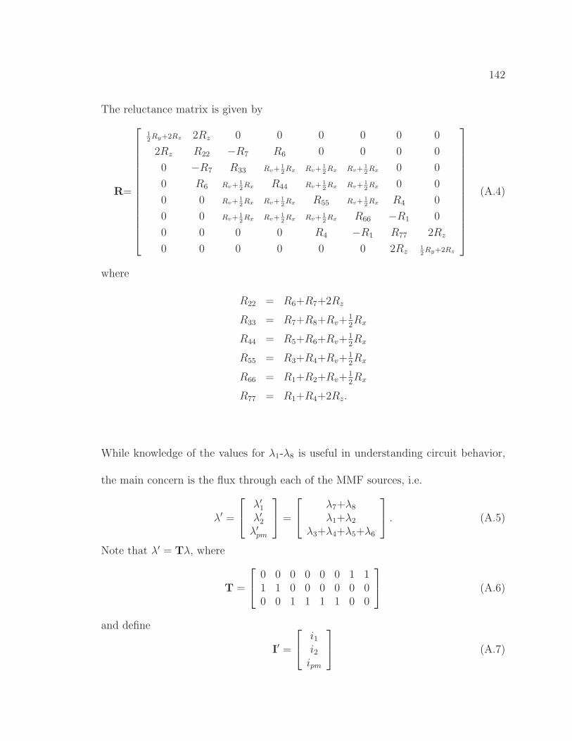
142

The reluctance matrix is given by

R=

1

2Ry+2Rz 2Rz 0 0 0 0 0 0

2Rz R22 −R7 R6 0 0 0 0

0 −R7 R33 Rv+ 1

2Rx Rv+ 1

2Rx Rv+ 1

2Rx 0 0

0 R6 Rv+ 1

2Rx R44 Rv+ 1

2Rx Rv+ 1

2Rx 0 0

0 0 Rv+ 1

2Rx Rv+ 1

2Rx R55 Rv+ 1

2Rx R4 0

0 0 Rv+ 1

2Rx Rv+ 1

2Rx Rv+ 1

2Rx R66 −R1 0

0 0 0 0 R4 −R1 R77 2Rz

0 0 0 0 0 0 2Rz1

2Ry+2Rz

(A.4)

where

R22 = R6+R7+2Rz

R33 = R7+R8+Rv+12Rx

R44 = R5+R6+Rv+12Rx

R55 = R3+R4+Rv+12Rx

R66 = R1+R2+Rv+12Rx

R77 = R1+R4+2Rz.

While knowledge of the values for λ1-λ8 is useful in understanding circuit behavior,

the main concern is the flux through each of the MMF sources, i.e.

λ′ =

λ′1

λ′2

λ′pm

=

λ7+λ8

λ1+λ2

λ3+λ4+λ5+λ6

. (A.5)

Note that λ′ = Tλ, where

T =

0 0 0 0 0 0 1 11 1 0 0 0 0 0 00 0 1 1 1 1 0 0

(A.6)

and define

I′ =

i1i2ipm

(A.7)

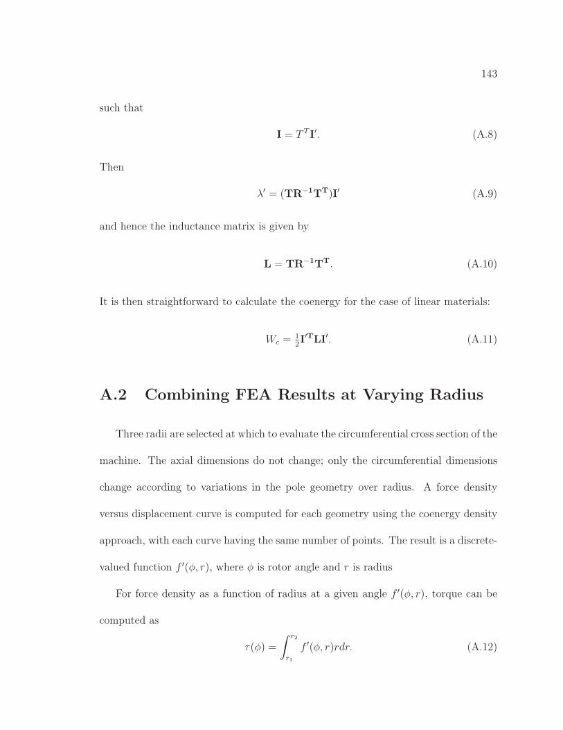
143

such that

I = T T I′. (A.8)

Then

λ′ = (TR−1TT)I′ (A.9)

and hence the inductance matrix is given by

L = TR−1TT. (A.10)

It is then straightforward to calculate the coenergy for the case of linear materials:

Wc = 12I′TLI′. (A.11)

A.2 Combining FEA Results at Varying Radius

Three radii are selected at which to evaluate the circumferential cross section of the

machine. The axial dimensions do not change; only the circumferential dimensions

change according to variations in the pole geometry over radius. A force density

versus displacement curve is computed for each geometry using the coenergy density

approach, with each curve having the same number of points. The result is a discrete-

valued function f ′(φ, r), where φ is rotor angle and r is radius

For force density as a function of radius at a given angle f ′(φ, r), torque can be

computed as

τ(φ) =

∫ r2

r1

f ′(φ, r)rdr. (A.12)

144

A second-order polynomial was selected to fit to the discrete f ′(φ, r) data points at

each value of φ. At a given rotor angular position, the function described above gives

three force density values at different radii: f ′(r1), f ′(r2), f ′(r3). The polynomial fit

must satisfy

f ′(φ, r1)

f ′(φ, r2)

f ′(φ, r3)

=

r21 r1 1

r22 r2 1

r23 r3 1

a1

a2

a3

(A.13)

where a1-a3 are the polynomial coefficients. Solving for the coefficients gives

~a = r−1 ~f. (A.14)

Now, substituting the polynomial into Eq. A.12 gives

τ =

∫ r3

r1

(a1r2 + a2r + a3r)rdr, (A.15)

which evaluates to

τ = (a1

4)(r4

3 − r41) + (

a2

3)(r3

3 − r31) + (

a3

2)(r2

3 − r21). (A.16)

A.3 Coenergy Density in Nonlinear Materials

The coenergy density within the nonlinear soft magnetic material included in the

FEA model of Ch. 6 can be found by evaluating the integral

W ′c =

∫

B(H) · dH. (A.17)

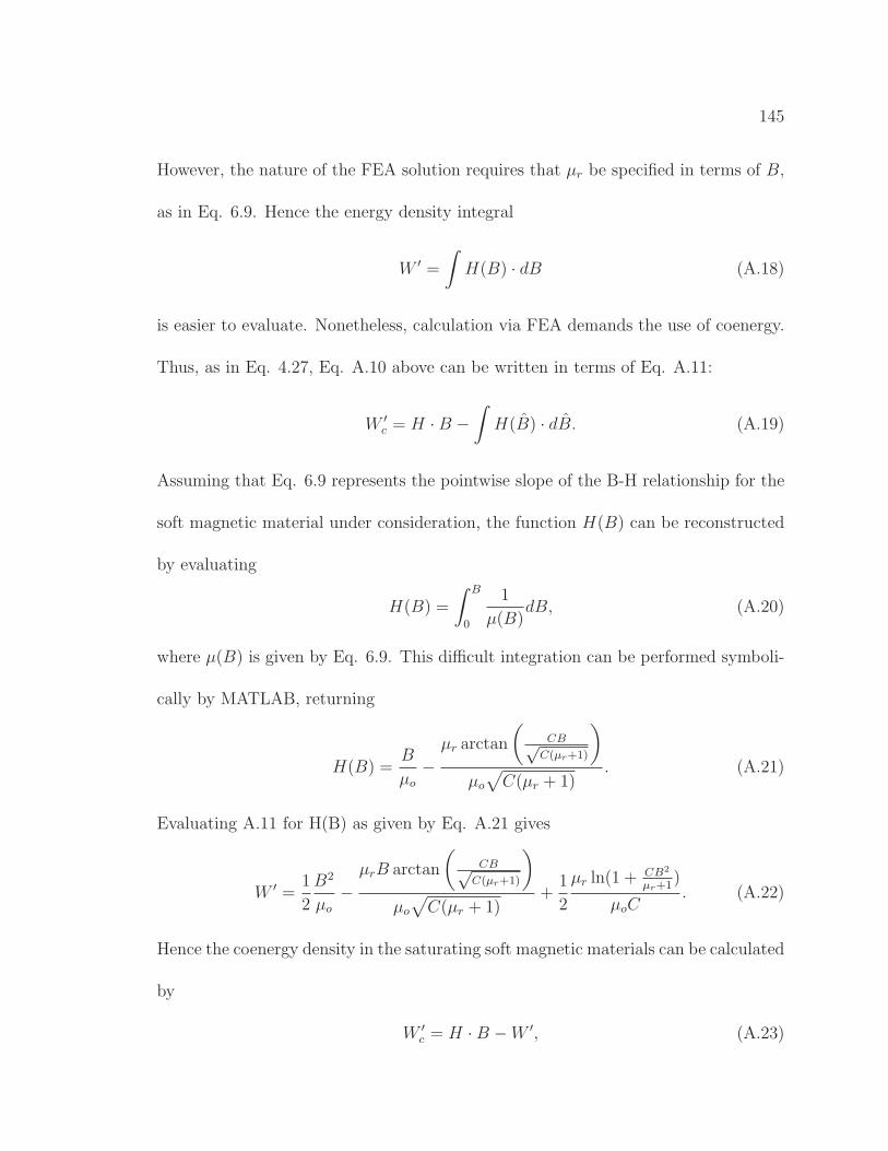
145

However, the nature of the FEA solution requires that µr be specified in terms of B,

as in Eq. 6.9. Hence the energy density integral

W ′ =

∫

H(B) · dB (A.18)

is easier to evaluate. Nonetheless, calculation via FEA demands the use of coenergy.

Thus, as in Eq. 4.27, Eq. A.10 above can be written in terms of Eq. A.11:

W ′c = H · B −

∫

H(B) · dB. (A.19)

Assuming that Eq. 6.9 represents the pointwise slope of the B-H relationship for the

soft magnetic material under consideration, the function H(B) can be reconstructed

by evaluating

H(B) =

∫ B

0

1

µ(B)dB, (A.20)

where µ(B) is given by Eq. 6.9. This difficult integration can be performed symboli-

cally by MATLAB, returning

H(B) =B

µo

−µr arctan

(

CB√C(µr+1)

)

µo

√

C(µr + 1). (A.21)

Evaluating A.11 for H(B) as given by Eq. A.21 gives

W ′ =1

2

B2

µo

−µrB arctan

(

CB√C(µr+1)

)

µo

√

C(µr + 1)+

1

2

µr ln(1 + CB2

µr+1)

µoC. (A.22)

Hence the coenergy density in the saturating soft magnetic materials can be calculated

by

W ′c = H · B − W ′, (A.23)

146

where W ′ is given by Eq. A.22. And finally, coenergy can be found by integrating

coenergy density over volume, as in Eq. 4.44.

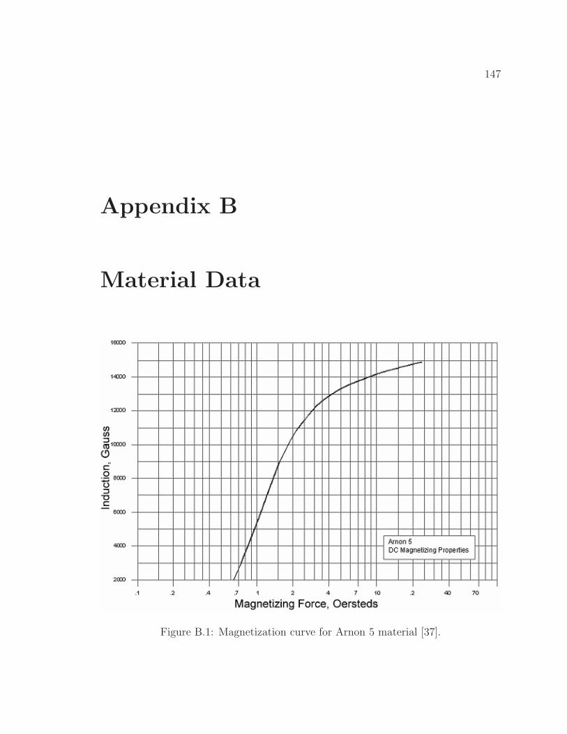
147

Appendix B

Material Data

Figure B.1: Magnetization curve for Arnon 5 material [37].

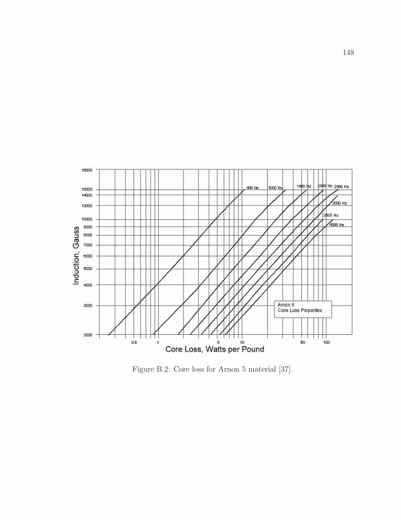
148

Figure B.2: Core loss for Arnon 5 material [37].

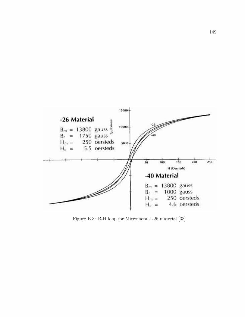
149

Figure B.3: B-H loop for Micrometals -26 material [38].

150

Figure B.4: Permeability versus field intensity for Micrometals -26 material [38].

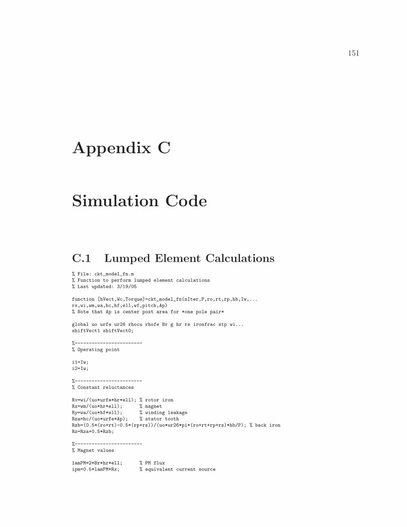
151

Appendix C

Simulation Code

C.1 Lumped Element Calculations

% File: ckt_model_fn.m

% Function to perform lumped element calculations

% Last updated: 3/19/05

function [hVect,Wc,Torque]=ckt_model_fn(nIter,P,ro,rt,rp,hb,Iw,...

rx,wi,wm,wa,hc,hf,ell,wf,pitch,Ap)

% Note that Ap is center post area for *one pole pair*

global uo urfe ur26 rhocu rhofe Br g hr rs ironfrac stp wi...

shiftVect1 shiftVect0;

%------------------------

% Operating point

i1=Iw;

i2=Iw;

%------------------------

% Constant reluctances

Rv=wi/(uo*urfe*hr*ell); % rotor iron

Rx=wm/(uo*hr*ell); % magnet

Ry=wa/(uo*hf*ell); % winding leakage

Rza=hc/(uo*urfe*Ap); % stator tooth

Rzb=(0.5*(ro+rt)-0.5*(rp+rs))/(uo*ur26*pi*(ro+rt+rp+rs)*hb/P); % back iron

Rz=Rza+0.5*Rzb;

%------------------------

% Magnet values

lamPM=2*Br*hr*ell; % PM flux

ipm=0.5*lamPM*Rx; % equivalent current source

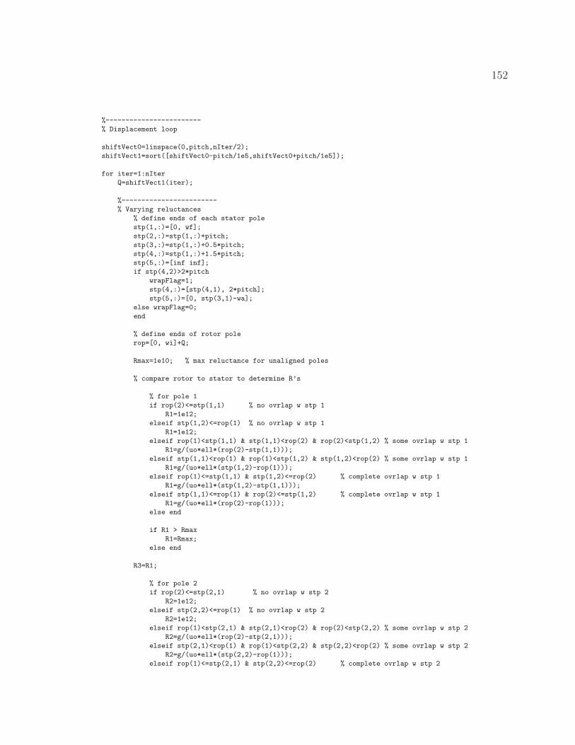
152

%------------------------

% Displacement loop

shiftVect0=linspace(0,pitch,nIter/2);

shiftVect1=sort([shiftVect0-pitch/1e5,shiftVect0+pitch/1e5]);

for iter=1:nIter

Q=shiftVect1(iter);

%------------------------

% Varying reluctances

% define ends of each stator pole

stp(1,:)=[0, wf];

stp(2,:)=stp(1,:)+pitch;

stp(3,:)=stp(1,:)+0.5*pitch;

stp(4,:)=stp(1,:)+1.5*pitch;

stp(5,:)=[inf inf];

if stp(4,2)>2*pitch

wrapFlag=1;

stp(4,:)=[stp(4,1), 2*pitch];

stp(5,:)=[0, stp(3,1)-wa];

else wrapFlag=0;

end

% define ends of rotor pole

rop=[0, wi]+Q;

Rmax=1e10; % max reluctance for unaligned poles

% compare rotor to stator to determine R’s

% for pole 1

if rop(2)<=stp(1,1) % no ovrlap w stp 1

R1=1e12;

elseif stp(1,2)<=rop(1) % no ovrlap w stp 1

R1=1e12;

elseif rop(1)<stp(1,1) & stp(1,1)<rop(2) & rop(2)<stp(1,2) % some ovrlap w stp 1

R1=g/(uo*ell*(rop(2)-stp(1,1)));

elseif stp(1,1)<rop(1) & rop(1)<stp(1,2) & stp(1,2)<rop(2) % some ovrlap w stp 1

R1=g/(uo*ell*(stp(1,2)-rop(1)));

elseif rop(1)<=stp(1,1) & stp(1,2)<=rop(2) % complete ovrlap w stp 1

R1=g/(uo*ell*(stp(1,2)-stp(1,1)));

elseif stp(1,1)<=rop(1) & rop(2)<=stp(1,2) % complete ovrlap w stp 1

R1=g/(uo*ell*(rop(2)-rop(1)));

else end

if R1 > Rmax

R1=Rmax;

else end

R3=R1;

% for pole 2

if rop(2)<=stp(2,1) % no ovrlap w stp 2

R2=1e12;

elseif stp(2,2)<=rop(1) % no ovrlap w stp 2

R2=1e12;

elseif rop(1)<stp(2,1) & stp(2,1)<rop(2) & rop(2)<stp(2,2) % some ovrlap w stp 2

R2=g/(uo*ell*(rop(2)-stp(2,1)));

elseif stp(2,1)<rop(1) & rop(1)<stp(2,2) & stp(2,2)<rop(2) % some ovrlap w stp 2

R2=g/(uo*ell*(stp(2,2)-rop(1)));

elseif rop(1)<=stp(2,1) & stp(2,2)<=rop(2) % complete ovrlap w stp 2

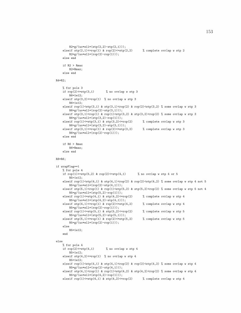
153

R2=g/(uo*ell*(stp(2,2)-stp(2,1)));

elseif stp(2,1)<=rop(1) & rop(2)<=stp(2,2) % complete ovrlap w stp 2

R2=g/(uo*ell*(rop(2)-rop(1)));

else end

if R2 > Rmax

R2=Rmax;

else end

R4=R2;

% for pole 3

if rop(2)<=stp(3,1) % no ovrlap w stp 3

R6=1e12;

elseif stp(3,2)<=rop(1) % no ovrlap w stp 3

R6=1e12;

elseif rop(1)<stp(3,1) & stp(3,1)<rop(2) & rop(2)<stp(3,2) % some ovrlap w stp 3

R6=g/(uo*ell*(rop(2)-stp(3,1)));

elseif stp(3,1)<rop(1) & rop(1)<stp(3,2) & stp(3,2)<rop(2) % some ovrlap w stp 3

R6=g/(uo*ell*(stp(3,2)-rop(1)));

elseif rop(1)<=stp(3,1) & stp(3,2)<=rop(2) % complete ovrlap w stp 3

R6=g/(uo*ell*(stp(3,2)-stp(3,1)));

elseif stp(3,1)<=rop(1) & rop(2)<=stp(3,2) % complete ovrlap w stp 3

R6=g/(uo*ell*(rop(2)-rop(1)));

else end

if R6 > Rmax

R6=Rmax;

else end

R8=R6;

if wrapFlag==1

% for pole 4

if rop(1)>=stp(5,2) & rop(2)<=stp(4,1) % no ovrlap w stp 4 or 5

R5=1e12;

elseif rop(1)<stp(4,1) & stp(4,1)<rop(2) & rop(2)<stp(4,2) % some ovrlap w stp 4 not 5

R5=g/(uo*ell*(rop(2)-stp(4,1)));

elseif stp(5,1)<rop(1) & rop(1)<stp(5,2) & stp(5,2)<rop(2) % some ovrlap w stp 5 not 4

R5=g/(uo*ell*(stp(5,2)-rop(1)));

elseif rop(1)<=stp(4,1) & stp(4,2)<=rop(2) % complete ovrlap w stp 4

R5=g/(uo*ell*(stp(4,2)-stp(4,1)));

elseif stp(4,1)<=rop(1) & rop(2)<=stp(4,2) % complete ovrlap w stp 4

R5=g/(uo*ell*(rop(2)-rop(1)));

elseif rop(1)<=stp(5,1) & stp(5,2)<=rop(2) % complete ovrlap w stp 5

R5=g/(uo*ell*(stp(5,2)-stp(5,1)));

elseif stp(5,1)<=rop(1) & rop(2)<=stp(5,2) % complete ovrlap w stp 5

R5=g/(uo*ell*(rop(2)-rop(1)));

else

R5=1e12;

end

else

% for pole 4

if rop(2)<=stp(4,1) % no ovrlap w stp 4

R5=1e12;

elseif stp(4,2)<=rop(1) % no ovrlap w stp 4

R5=1e12;

elseif rop(1)<stp(4,1) & stp(4,1)<rop(2) & rop(2)<stp(4,2) % some ovrlap w stp 4

R5=g/(uo*ell*(rop(2)-stp(4,1)));

elseif stp(4,1)<rop(1) & rop(1)<stp(4,2) & stp(4,2)<rop(2) % some ovrlap w stp 4

R5=g/(uo*ell*(stp(4,2)-rop(1)));

elseif rop(1)<=stp(4,1) & stp(4,2)<=rop(2) % complete ovrlap w stp 4

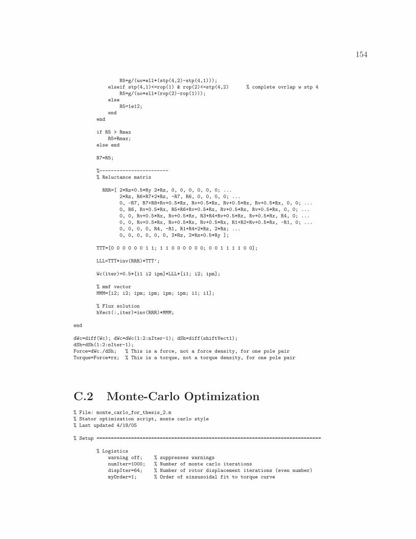
154

R5=g/(uo*ell*(stp(4,2)-stp(4,1)));

elseif stp(4,1)<=rop(1) & rop(2)<=stp(4,2) % complete ovrlap w stp 4

R5=g/(uo*ell*(rop(2)-rop(1)));

else

R5=1e12;

end

end

if R5 > Rmax

R5=Rmax;

else end

R7=R5;

%------------------------

% Reluctance matrix

RRR=[ 2*Rz+0.5*Ry 2*Rz, 0, 0, 0, 0, 0, 0; ...

2*Rz, R6+R7+2*Rz, -R7, R6, 0, 0, 0, 0; ...

0, -R7, R7+R8+Rv+0.5*Rx, Rv+0.5*Rx, Rv+0.5*Rx, Rv+0.5*Rx, 0, 0; ...

0, R6, Rv+0.5*Rx, R5+R6+Rv+0.5*Rx, Rv+0.5*Rx, Rv+0.5*Rx, 0, 0; ...

0, 0, Rv+0.5*Rx, Rv+0.5*Rx, R3+R4+Rv+0.5*Rx, Rv+0.5*Rx, R4, 0; ...

0, 0, Rv+0.5*Rx, Rv+0.5*Rx, Rv+0.5*Rx, R1+R2+Rv+0.5*Rx, -R1, 0; ...

0, 0, 0, 0, R4, -R1, R1+R4+2*Rz, 2*Rz; ...

0, 0, 0, 0, 0, 0, 2*Rz, 2*Rz+0.5*Ry ];

TTT=[0 0 0 0 0 0 1 1; 1 1 0 0 0 0 0 0; 0 0 1 1 1 1 0 0];

LLL=TTT*inv(RRR)*TTT’;

Wc(iter)=0.5*[i1 i2 ipm]*LLL*[i1; i2; ipm];

% mmf vector

MMM=[i2; i2; ipm; ipm; ipm; ipm; i1; i1];

% Flux solution

hVect(:,iter)=inv(RRR)*MMM;

end

dWc=diff(Wc); dWc=dWc(1:2:nIter-1); dSh=diff(shiftVect1);

dSh=dSh(1:2:nIter-1);

Force=dWc./dSh; % This is a force, not a force density, for one pole pair

Torque=Force*rx; % This is a torque, not a torque density, for one pole pair

C.2 Monte-Carlo Optimization

% File: monte_carlo_for_thesis_2.m

% Stator optimization script, monte carlo style

% Last updated 4/18/05

% Setup ==============================================================================

% Logistics

warning off; % suppresses warnings

numIter=1000; % Number of monte carlo iterations

dispIter=64; % Number of rotor displacement iterations (even number)

myOrder=1; % Order of sinsusoidal fit to torque curve

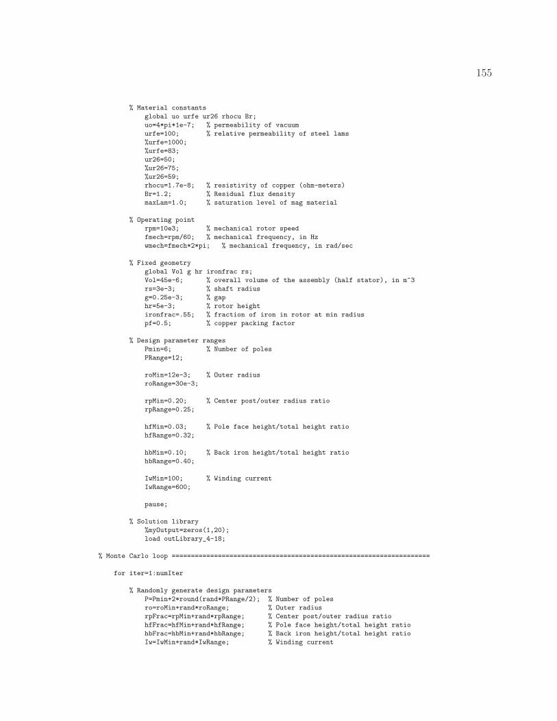
155

% Material constants

global uo urfe ur26 rhocu Br;

uo=4*pi*1e-7; % permeability of vacuum

urfe=100; % relative permeability of steel lams

%urfe=1000;

%urfe=83;

ur26=50;

%ur26=75;

%ur26=59;

rhocu=1.7e-8; % resistivity of copper (ohm-meters)

Br=1.2; % Residual flux density

maxLam=1.0; % saturation level of mag material

% Operating point

rpm=10e3; % mechanical rotor speed

fmech=rpm/60; % mechanical frequency, in Hz

wmech=fmech*2*pi; % mechanical frequency, in rad/sec

% Fixed geometry

global Vol g hr ironfrac rs;

Vol=45e-6; % overall volume of the assembly (half stator), in m^3

rs=3e-3; % shaft radius

g=0.25e-3; % gap

hr=5e-3; % rotor height

ironfrac=.55; % fraction of iron in rotor at min radius

pf=0.5; % copper packing factor

% Design parameter ranges

Pmin=6; % Number of poles

PRange=12;

roMin=12e-3; % Outer radius

roRange=30e-3;

rpMin=0.20; % Center post/outer radius ratio

rpRange=0.25;

hfMin=0.03; % Pole face height/total height ratio

hfRange=0.32;

hbMin=0.10; % Back iron height/total height ratio

hbRange=0.40;

IwMin=100; % Winding current

IwRange=600;

pause;

% Solution library

%myOutput=zeros(1,20);

load outLibrary_4-18;

% Monte Carlo loop ===================================================================

for iter=1:numIter

% Randomly generate design parameters

P=Pmin+2*round(rand*PRange/2); % Number of poles

ro=roMin+rand*roRange; % Outer radius

rpFrac=rpMin+rand*rpRange; % Center post/outer radius ratio

hfFrac=hfMin+rand*hfRange; % Pole face height/total height ratio

hbFrac=hbMin+rand*hbRange; % Back iron height/total height ratio

Iw=IwMin+rand*IwRange; % Winding current

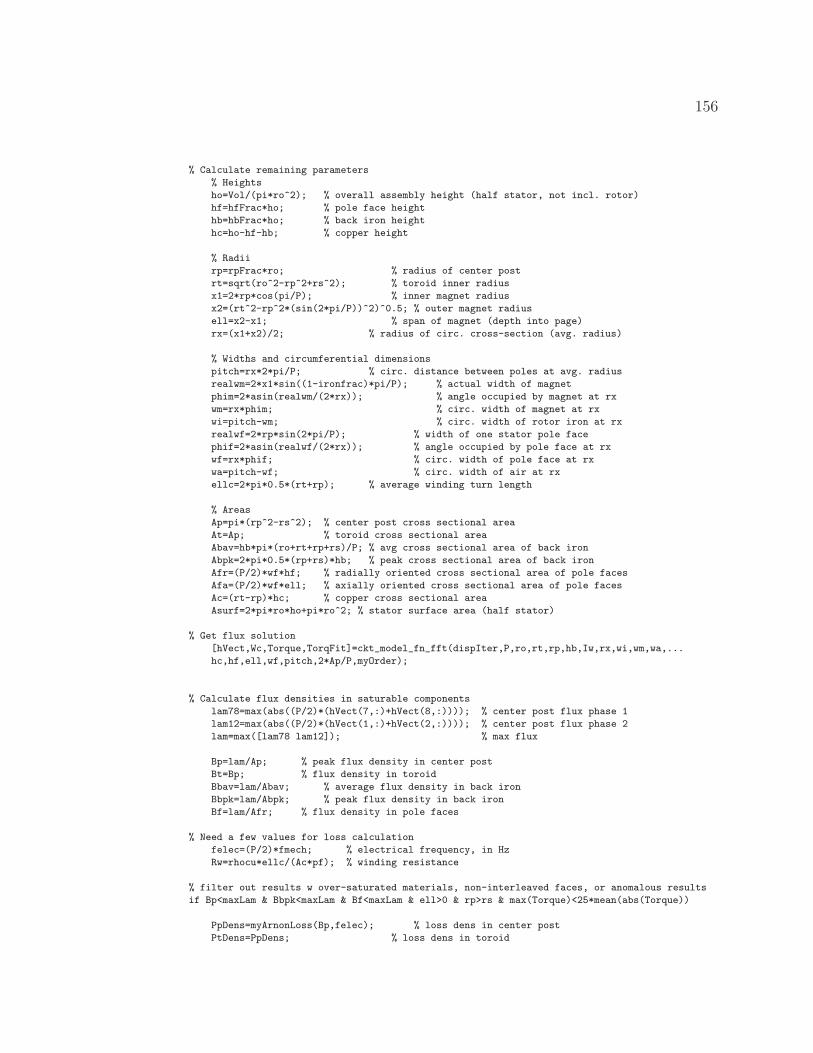
156

% Calculate remaining parameters

% Heights

ho=Vol/(pi*ro^2); % overall assembly height (half stator, not incl. rotor)

hf=hfFrac*ho; % pole face height

hb=hbFrac*ho; % back iron height

hc=ho-hf-hb; % copper height

% Radii

rp=rpFrac*ro; % radius of center post

rt=sqrt(ro^2-rp^2+rs^2); % toroid inner radius

x1=2*rp*cos(pi/P); % inner magnet radius

x2=(rt^2-rp^2*(sin(2*pi/P))^2)^0.5; % outer magnet radius

ell=x2-x1; % span of magnet (depth into page)

rx=(x1+x2)/2; % radius of circ. cross-section (avg. radius)

% Widths and circumferential dimensions

pitch=rx*2*pi/P; % circ. distance between poles at avg. radius

realwm=2*x1*sin((1-ironfrac)*pi/P); % actual width of magnet

phim=2*asin(realwm/(2*rx)); % angle occupied by magnet at rx

wm=rx*phim; % circ. width of magnet at rx

wi=pitch-wm; % circ. width of rotor iron at rx

realwf=2*rp*sin(2*pi/P); % width of one stator pole face

phif=2*asin(realwf/(2*rx)); % angle occupied by pole face at rx

wf=rx*phif; % circ. width of pole face at rx

wa=pitch-wf; % circ. width of air at rx

ellc=2*pi*0.5*(rt+rp); % average winding turn length

% Areas

Ap=pi*(rp^2-rs^2); % center post cross sectional area

At=Ap; % toroid cross sectional area

Abav=hb*pi*(ro+rt+rp+rs)/P; % avg cross sectional area of back iron

Abpk=2*pi*0.5*(rp+rs)*hb; % peak cross sectional area of back iron

Afr=(P/2)*wf*hf; % radially oriented cross sectional area of pole faces

Afa=(P/2)*wf*ell; % axially oriented cross sectional area of pole faces

Ac=(rt-rp)*hc; % copper cross sectional area

Asurf=2*pi*ro*ho+pi*ro^2; % stator surface area (half stator)

% Get flux solution

[hVect,Wc,Torque,TorqFit]=ckt_model_fn_fft(dispIter,P,ro,rt,rp,hb,Iw,rx,wi,wm,wa,...

hc,hf,ell,wf,pitch,2*Ap/P,myOrder);

% Calculate flux densities in saturable components

lam78=max(abs((P/2)*(hVect(7,:)+hVect(8,:)))); % center post flux phase 1

lam12=max(abs((P/2)*(hVect(1,:)+hVect(2,:)))); % center post flux phase 2

lam=max([lam78 lam12]); % max flux

Bp=lam/Ap; % peak flux density in center post

Bt=Bp; % flux density in toroid

Bbav=lam/Abav; % average flux density in back iron

Bbpk=lam/Abpk; % peak flux density in back iron

Bf=lam/Afr; % flux density in pole faces

% Need a few values for loss calculation

felec=(P/2)*fmech; % electrical frequency, in Hz

Rw=rhocu*ellc/(Ac*pf); % winding resistance

% filter out results w over-saturated materials, non-interleaved faces, or anomalous results

if Bp<maxLam & Bbpk<maxLam & Bf<maxLam & ell>0 & rp>rs & max(Torque)<25*mean(abs(Torque))

PpDens=myArnonLoss(Bp,felec); % loss dens in center post

PtDens=PpDens; % loss dens in toroid

157

PbDens=myMicrometLoss(Bbav,felec); % loss dens in back iron (use average flux density)

PfDens=myArnonLoss(Bf,felec); % loss dens in pole faces

volP=Ap*hc; % volume of center post (half stator)

volT=volP; % volume of toroid (half stator)

volB=Abav*(0.5*(ro+rt)-0.5*(rp+rs)); % effective volume of back iron (half stator)

volF=2*Afr*(ro-rs); % approximate volume of pole faces (overestimates)

% Power calculations =================================================

Pp=PpDens*volP; % core loss in center post (half stator)

Pt=PtDens*volT; % core loss in toroid (half stator)

Pb=PbDens*volB; % core loss in back iron (half stator)

Pf=PfDens*volF; % core loss in pole faces (half stator)

Pcore=2*(Pp+Pt+Pb+Pf); % total core loss (whole machine)

Pmech=(P/2)*max(abs(TorqFit))*wmech; % Mechanical power (whole machine)

Pcu=2*Iw^2*Rw; % conduction loss (whole machine)

Pout=Pmech-Pcu-Pcore; % Net power (whole machine)

eta=Pout/Pmech; % efficiency

% Check list

dropFlag=0;

for nchk=1:size(myOutput)*[1;0]

if (myOutput(nchk,1) < Pout | myOutput(nchk,2) < eta)

% point is approved if it has superior Pout OR eta, AND is thermally acceptable

else

dropFlag=1;

end % if

end % for

if dropFlag==0

% Purge list

ntemp=1;

tempOutput=[];

for npur=1:size(myOutput)*[1;0]

if myOutput(npur,1) < Pout & myOutput(npur,2) < eta

plot(myOutput(npur,2), myOutput(npur,1),’rx’);

hold on;

else

tempOutput(ntemp,:)=myOutput(npur,:); % keep good points

ntemp=ntemp+1;

end % if

end % for

myOutput=tempOutput;

% Save point

myOutput(size(myOutput)*[1;0]+1,:)=[Pout,eta,P,ro,rp,rt,rx,ho,hf,hb,hc,Ap,Bp,Bt,...

Bbpk,Bf,Iw,Pcore,Pcu,(Pcore+Pcu)/(2*Asurf)];

plot(eta, Pout,’ko’);

hold on;

else end % if dropFlag==0

else

end % if Bp<1 etc

end % for

save outLibrary_4-19 myOutput;

%

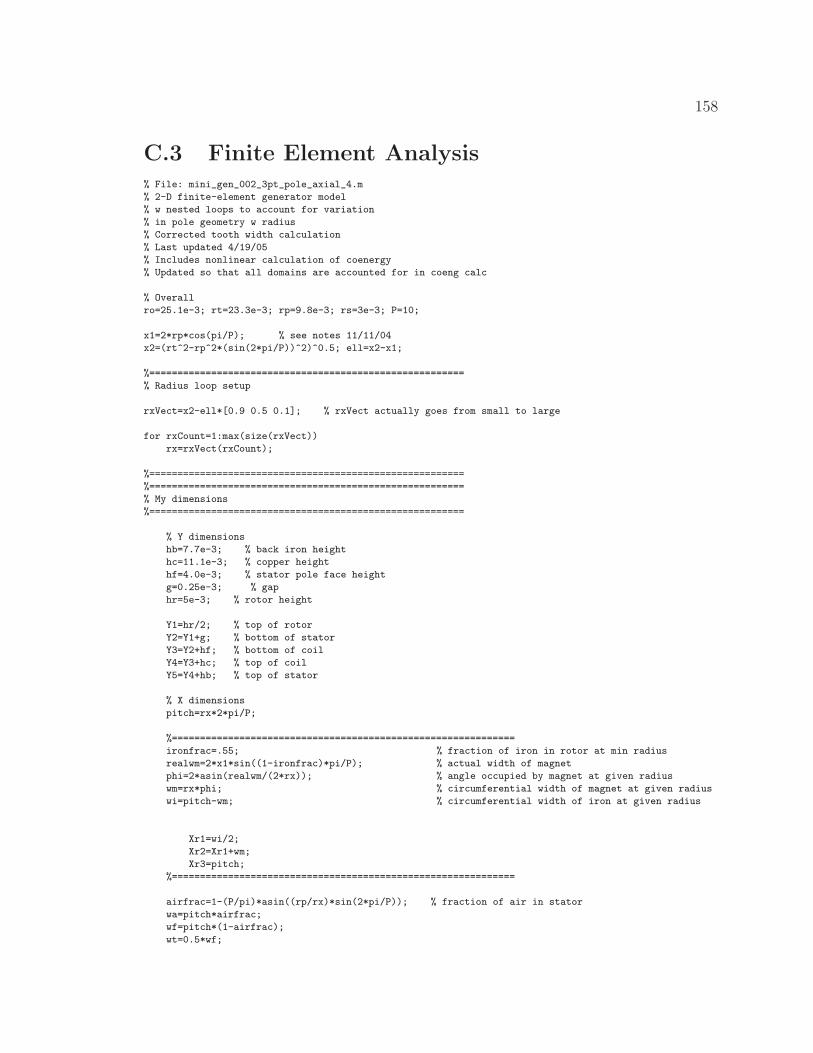
158

C.3 Finite Element Analysis

% File: mini_gen_002_3pt_pole_axial_4.m

% 2-D finite-element generator model

% w nested loops to account for variation

% in pole geometry w radius

% Corrected tooth width calculation

% Last updated 4/19/05

% Includes nonlinear calculation of coenergy

% Updated so that all domains are accounted for in coeng calc

% Overall

ro=25.1e-3; rt=23.3e-3; rp=9.8e-3; rs=3e-3; P=10;

x1=2*rp*cos(pi/P); % see notes 11/11/04

x2=(rt^2-rp^2*(sin(2*pi/P))^2)^0.5; ell=x2-x1;

%========================================================

% Radius loop setup

rxVect=x2-ell*[0.9 0.5 0.1]; % rxVect actually goes from small to large

for rxCount=1:max(size(rxVect))

rx=rxVect(rxCount);

%========================================================

%========================================================

% My dimensions

%========================================================

% Y dimensions

hb=7.7e-3; % back iron height

hc=11.1e-3; % copper height

hf=4.0e-3; % stator pole face height

g=0.25e-3; % gap

hr=5e-3; % rotor height

Y1=hr/2; % top of rotor

Y2=Y1+g; % bottom of stator

Y3=Y2+hf; % bottom of coil

Y4=Y3+hc; % top of coil

Y5=Y4+hb; % top of stator

% X dimensions

pitch=rx*2*pi/P;

%=============================================================

ironfrac=.55; % fraction of iron in rotor at min radius

realwm=2*x1*sin((1-ironfrac)*pi/P); % actual width of magnet

phi=2*asin(realwm/(2*rx)); % angle occupied by magnet at given radius

wm=rx*phi; % circumferential width of magnet at given radius

wi=pitch-wm; % circumferential width of iron at given radius

Xr1=wi/2;

Xr2=Xr1+wm;

Xr3=pitch;

%=============================================================

airfrac=1-(P/pi)*asin((rp/rx)*sin(2*pi/P)); % fraction of air in stator

wa=pitch*airfrac;

wf=pitch*(1-airfrac);

wt=0.5*wf;

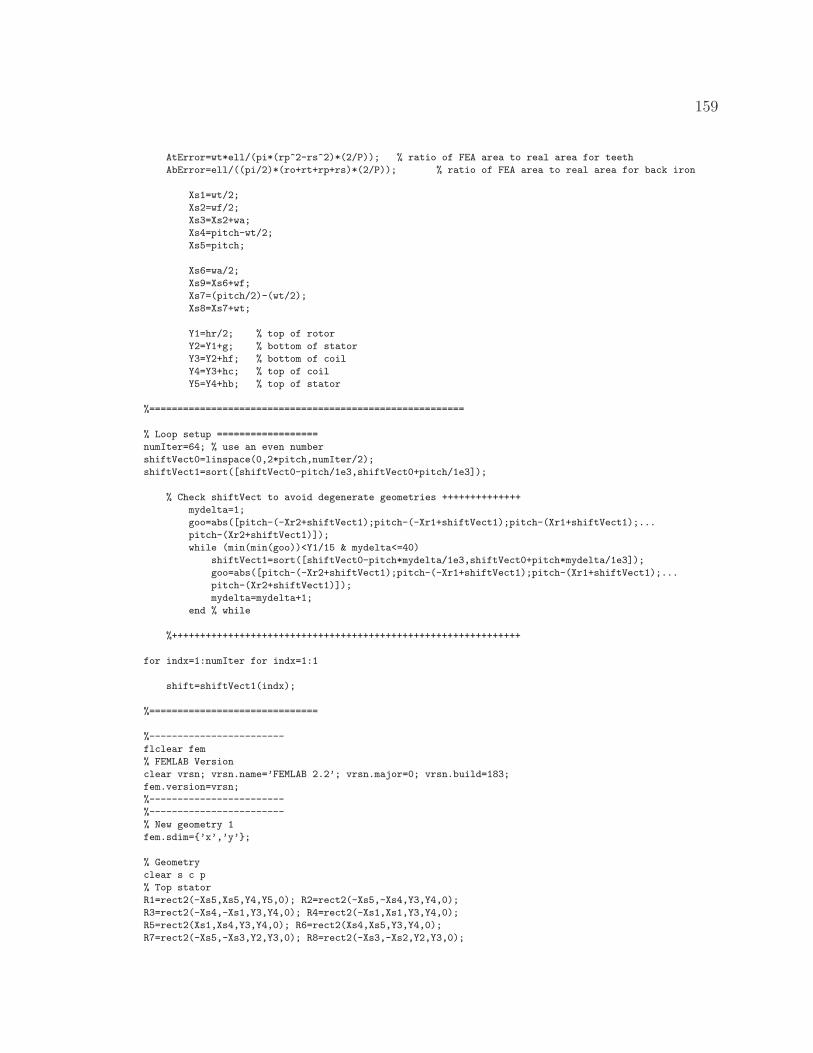
159

AtError=wt*ell/(pi*(rp^2-rs^2)*(2/P)); % ratio of FEA area to real area for teeth

AbError=ell/((pi/2)*(ro+rt+rp+rs)*(2/P)); % ratio of FEA area to real area for back iron

Xs1=wt/2;

Xs2=wf/2;

Xs3=Xs2+wa;

Xs4=pitch-wt/2;

Xs5=pitch;

Xs6=wa/2;

Xs9=Xs6+wf;

Xs7=(pitch/2)-(wt/2);

Xs8=Xs7+wt;

Y1=hr/2; % top of rotor

Y2=Y1+g; % bottom of stator

Y3=Y2+hf; % bottom of coil

Y4=Y3+hc; % top of coil

Y5=Y4+hb; % top of stator

%========================================================

% Loop setup ==================

numIter=64; % use an even number

shiftVect0=linspace(0,2*pitch,numIter/2);

shiftVect1=sort([shiftVect0-pitch/1e3,shiftVect0+pitch/1e3]);

% Check shiftVect to avoid degenerate geometries ++++++++++++++

mydelta=1;

goo=abs([pitch-(-Xr2+shiftVect1);pitch-(-Xr1+shiftVect1);pitch-(Xr1+shiftVect1);...

pitch-(Xr2+shiftVect1)]);

while (min(min(goo))<Y1/15 & mydelta<=40)

shiftVect1=sort([shiftVect0-pitch*mydelta/1e3,shiftVect0+pitch*mydelta/1e3]);

goo=abs([pitch-(-Xr2+shiftVect1);pitch-(-Xr1+shiftVect1);pitch-(Xr1+shiftVect1);...

pitch-(Xr2+shiftVect1)]);

mydelta=mydelta+1;

end % while

%++++++++++++++++++++++++++++++++++++++++++++++++++++++++++++++

for indx=1:numIter for indx=1:1

shift=shiftVect1(indx);

%==============================

%------------------------

flclear fem

% FEMLAB Version

clear vrsn; vrsn.name=’FEMLAB 2.2’; vrsn.major=0; vrsn.build=183;

fem.version=vrsn;

%------------------------

%------------------------

% New geometry 1

fem.sdim=’x’,’y’;

% Geometry

clear s c p

% Top stator

R1=rect2(-Xs5,Xs5,Y4,Y5,0); R2=rect2(-Xs5,-Xs4,Y3,Y4,0);

R3=rect2(-Xs4,-Xs1,Y3,Y4,0); R4=rect2(-Xs1,Xs1,Y3,Y4,0);

R5=rect2(Xs1,Xs4,Y3,Y4,0); R6=rect2(Xs4,Xs5,Y3,Y4,0);

R7=rect2(-Xs5,-Xs3,Y2,Y3,0); R8=rect2(-Xs3,-Xs2,Y2,Y3,0);

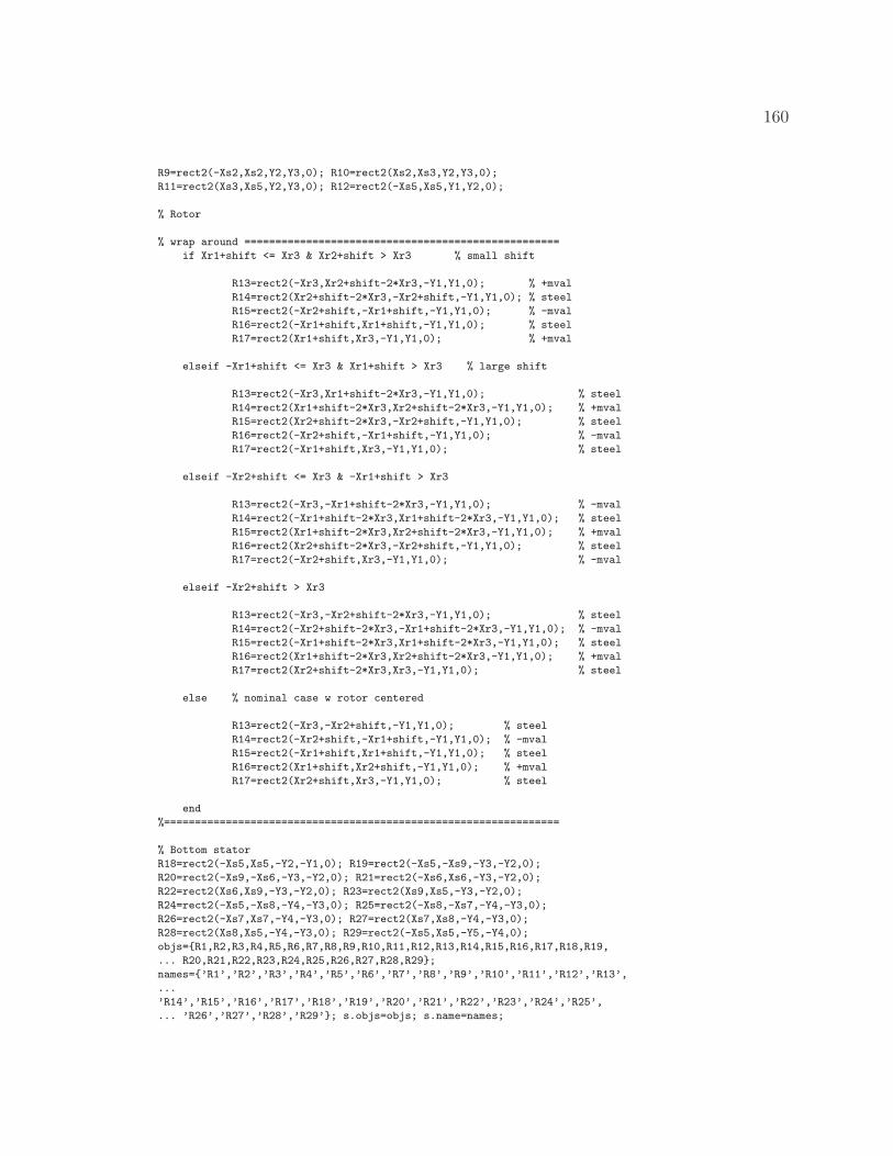
160

R9=rect2(-Xs2,Xs2,Y2,Y3,0); R10=rect2(Xs2,Xs3,Y2,Y3,0);

R11=rect2(Xs3,Xs5,Y2,Y3,0); R12=rect2(-Xs5,Xs5,Y1,Y2,0);

% Rotor

% wrap around ===================================================

if Xr1+shift <= Xr3 & Xr2+shift > Xr3 % small shift

R13=rect2(-Xr3,Xr2+shift-2*Xr3,-Y1,Y1,0); % +mval

R14=rect2(Xr2+shift-2*Xr3,-Xr2+shift,-Y1,Y1,0); % steel

R15=rect2(-Xr2+shift,-Xr1+shift,-Y1,Y1,0); % -mval

R16=rect2(-Xr1+shift,Xr1+shift,-Y1,Y1,0); % steel

R17=rect2(Xr1+shift,Xr3,-Y1,Y1,0); % +mval

elseif -Xr1+shift <= Xr3 & Xr1+shift > Xr3 % large shift

R13=rect2(-Xr3,Xr1+shift-2*Xr3,-Y1,Y1,0); % steel

R14=rect2(Xr1+shift-2*Xr3,Xr2+shift-2*Xr3,-Y1,Y1,0); % +mval

R15=rect2(Xr2+shift-2*Xr3,-Xr2+shift,-Y1,Y1,0); % steel

R16=rect2(-Xr2+shift,-Xr1+shift,-Y1,Y1,0); % -mval

R17=rect2(-Xr1+shift,Xr3,-Y1,Y1,0); % steel

elseif -Xr2+shift <= Xr3 & -Xr1+shift > Xr3

R13=rect2(-Xr3,-Xr1+shift-2*Xr3,-Y1,Y1,0); % -mval

R14=rect2(-Xr1+shift-2*Xr3,Xr1+shift-2*Xr3,-Y1,Y1,0); % steel

R15=rect2(Xr1+shift-2*Xr3,Xr2+shift-2*Xr3,-Y1,Y1,0); % +mval

R16=rect2(Xr2+shift-2*Xr3,-Xr2+shift,-Y1,Y1,0); % steel

R17=rect2(-Xr2+shift,Xr3,-Y1,Y1,0); % -mval

elseif -Xr2+shift > Xr3

R13=rect2(-Xr3,-Xr2+shift-2*Xr3,-Y1,Y1,0); % steel

R14=rect2(-Xr2+shift-2*Xr3,-Xr1+shift-2*Xr3,-Y1,Y1,0); % -mval

R15=rect2(-Xr1+shift-2*Xr3,Xr1+shift-2*Xr3,-Y1,Y1,0); % steel

R16=rect2(Xr1+shift-2*Xr3,Xr2+shift-2*Xr3,-Y1,Y1,0); % +mval

R17=rect2(Xr2+shift-2*Xr3,Xr3,-Y1,Y1,0); % steel

else % nominal case w rotor centered

R13=rect2(-Xr3,-Xr2+shift,-Y1,Y1,0); % steel

R14=rect2(-Xr2+shift,-Xr1+shift,-Y1,Y1,0); % -mval

R15=rect2(-Xr1+shift,Xr1+shift,-Y1,Y1,0); % steel

R16=rect2(Xr1+shift,Xr2+shift,-Y1,Y1,0); % +mval

R17=rect2(Xr2+shift,Xr3,-Y1,Y1,0); % steel

end

%================================================================

% Bottom stator

R18=rect2(-Xs5,Xs5,-Y2,-Y1,0); R19=rect2(-Xs5,-Xs9,-Y3,-Y2,0);

R20=rect2(-Xs9,-Xs6,-Y3,-Y2,0); R21=rect2(-Xs6,Xs6,-Y3,-Y2,0);

R22=rect2(Xs6,Xs9,-Y3,-Y2,0); R23=rect2(Xs9,Xs5,-Y3,-Y2,0);

R24=rect2(-Xs5,-Xs8,-Y4,-Y3,0); R25=rect2(-Xs8,-Xs7,-Y4,-Y3,0);

R26=rect2(-Xs7,Xs7,-Y4,-Y3,0); R27=rect2(Xs7,Xs8,-Y4,-Y3,0);

R28=rect2(Xs8,Xs5,-Y4,-Y3,0); R29=rect2(-Xs5,Xs5,-Y5,-Y4,0);

objs=R1,R2,R3,R4,R5,R6,R7,R8,R9,R10,R11,R12,R13,R14,R15,R16,R17,R18,R19,

... R20,R21,R22,R23,R24,R25,R26,R27,R28,R29;

names=’R1’,’R2’,’R3’,’R4’,’R5’,’R6’,’R7’,’R8’,’R9’,’R10’,’R11’,’R12’,’R13’,

...

’R14’,’R15’,’R16’,’R17’,’R18’,’R19’,’R20’,’R21’,’R22’,’R23’,’R24’,’R25’,

... ’R26’,’R27’,’R28’,’R29’; s.objs=objs; s.name=names;

161

objs=; names=; c.objs=objs; c.name=names;

objs=; names=; p.objs=objs; p.name=names;

drawstruct=struct(’s’,s,’c’,c,’p’,p); fem.draw=drawstruct;

fem.geom=geomcsg(fem);

%------------------------

%===================================

% Domain group assignments for R’s

% 1=powdered iron (nonlin)

% 2=-ival (copper)

% 3=air

% 4=-mval(pm)

% 5=steel (no correction) (nonlin)

% 6=ival (copper)

% 7=mval (pm)

% 8=steel (w area correction) (nonlin)

% bot stator modified from original current configuration.

if Xr1+shift <= Xr3 & Xr2+shift > Xr3 % small shift

% 0 0 0 0 0 0 0 0 0 1 1 1 1 1 1 1 1 1 1 2 2 2 2 2 2 2 2 2 2

% 1 2 3 4 5 6 7 8 9 0 1 2 3 4 5 6 7 8 9 0 1 2 3 4 5 6 7 8 9

myRs = [1 8 6 8 2 8 5 3 5 3 5 3 7 5 4 5 7 3 3 5 3 5 3 6 8 2 8 6 1];

elseif -Xr1+shift <= Xr3 & Xr1+shift > Xr3 % large shift

% 0 0 0 0 0 0 0 0 0 1 1 1 1 1 1 1 1 1 1 2 2 2 2 2 2 2 2 2 2

% 1 2 3 4 5 6 7 8 9 0 1 2 3 4 5 6 7 8 9 0 1 2 3 4 5 6 7 8 9

myRs = [1 8 6 8 2 8 5 3 5 3 5 3 5 7 5 4 5 3 3 5 3 5 3 6 8 2 8 6 1];

elseif -Xr2+shift <= Xr3 & -Xr1+shift > Xr3

% 0 0 0 0 0 0 0 0 0 1 1 1 1 1 1 1 1 1 1 2 2 2 2 2 2 2 2 2 2

% 1 2 3 4 5 6 7 8 9 0 1 2 3 4 5 6 7 8 9 0 1 2 3 4 5 6 7 8 9

myRs = [1 8 6 8 2 8 5 3 5 3 5 3 4 5 7 5 4 3 3 5 3 5 3 6 8 2 8 6 1];

elseif -Xr2+shift > Xr3

% 0 0 0 0 0 0 0 0 0 1 1 1 1 1 1 1 1 1 1 2 2 2 2 2 2 2 2 2 2

% 1 2 3 4 5 6 7 8 9 0 1 2 3 4 5 6 7 8 9 0 1 2 3 4 5 6 7 8 9

myRs = [1 8 6 8 2 8 5 3 5 3 5 3 5 4 5 7 5 3 3 5 3 5 3 6 8 2 8 6 1];

else % nominal case w rotor centered

% 0 0 0 0 0 0 0 0 0 1 1 1 1 1 1 1 1 1 1 2 2 2 2 2 2 2 2 2 2

% 1 2 3 4 5 6 7 8 9 0 1 2 3 4 5 6 7 8 9 0 1 2 3 4 5 6 7 8 9

myRs = [1 8 6 8 2 8 5 3 5 3 5 3 5 4 5 7 5 3 3 5 3 5 3 6 8 2 8 6 1];

end

% Get mapping from R’s to subdomains (mySt is a sparse matrix)

mySt=geomcsg(fem,’Out’,’st’);

% Apply mapping to get domain group assignments for subdomains

mySubdomains=(full(mySt)*myRs’)’;

%===================================

%------------------------

clear appl

% Application mode 1

appl1.mode=flcemqap(’dim’,’Az’,’sdim’,’x’,’y’,’submode’,’t2’,’tdiff’,

... ’on’); appl1.name=’qap’; appl1.dim=’Az’;

appl1.border=’off’;

appl1.var=’epsilon0’,’8.854187817e-12’,’mu0’,’4*pi*1e-7’,’omega’,’0’;

appl1.form=’coefficient’; appl1.elemdefault=’Lag2’;

appl1.assign=’Bx’;’Bx_qap’;’By’;’By_qap’;’Dz’;’Dz_qap’;’Ez’;’Ez_qap’;

...

’Hx’;’Hx_qap’;’Hy’;’Hy_qap’;’Jez’;’Jez_qap’;’Jiz’;’Jiz_qap’;’Jvz’;’Jvz_qap’;

...

’Jz’;’Jz_qap’;’Mx’;’Mx_qap’;’My’;’My_qap’;’Poxav’;’Poxav_qap’;’Poyav’;

162

...

’Poyav_qap’;’Pz’;’Pz_qap’;’Qav’;’Qav_qap’;’Qiav’;’Qiav_qap’;’Qvav’;

...

’Qvav_qap’;’Wav’;’Wav_qap’;’Weav’;’Weav_qap’;’Wm’;’Wm_qap’;’Wmav’;

...

’Wmav_qap’;’eMx’;’eMx_qap’;’eMy’;’eMy_qap’;’ePz’;’ePz_qap’;’epsilon’;

...

’epsilon_qap’;’epsilon0’;’epsilon0_qap’;’mu’;’mu_qap’;’mu0’;’mu0_qap’;

...

’muxx’;’muxx_qap’;’muxy’;’muxy_qap’;’muyx’;’muyx_qap’;’muyy’;’muyy_qap’;

...

’nPoav’;’nPoav_qap’;’normB’;’normB_qap’;’normE’;’normE_qap’;’normH’;

...

’normH_qap’;’normJ’;’normJ_qap’;’omega’;’omega_qap’;’sigma’;’sigma_qap’;

... ’tH’;’tH_qap’;’vx’;’vx_qap’;’vy’;’vy_qap’;

appl1.shape=’shlag(2,’’Az’’)’; appl1.sshape=2;

appl1.equ.sigma=’0’,’0’,’0’,’0’,’0’,’0’,’0’,’0’;

appl1.equ.mur=’u26/(1+C3*normB_qap^2)+1’,’1’,’1’,’1’,

...

’uFe/(1+C*normB_qap^2)+1’,’1’,’1’,’uFe2/(1+C2*normB_qap^2)+1’;

appl1.equ.murtensor=’1’,’0’;’0’,’1’,’1’,’0’;’0’,’1’,’1’,’0’;

...

’0’,’1’,’1’,’0’;’0’,’1’,’1’,’0’;’0’,’1’,’1’,’0’;’0’,’1’,’1’,

... ’0’;’0’,’1’,’1’,’0’;’0’,’1’;

appl1.equ.M=’0’,’0’,’0’,’0’,’0’,’0’,’-mval’,’0’,’0’,

... ’0’,’0’,’0’,’mval’,’0’,’0’,’0’;

appl1.equ.Jext=’0’,’-ival’,’0’,’0’,’0’,’ival’,

... ’0’,’0’;

appl1.equ.v=’0’,’0’,’0’,’0’,’0’,’0’,’0’,’0’,’0’,’0’,

... ’0’,’0’,’0’,’0’,’0’,’0’;

appl1.equ.epsilonr=’1’,’1’,’1’,’1’,’1’,’1’,

... ’1’,’1’;

appl1.equ.P=’0’,’0’,’0’,’0’,’0’,’0’,’0’,’0’;

appl1.equ.mutype=’iso’,’iso’,’iso’,’iso’,’iso’,’iso’,’iso’,’iso’;

appl1.equ.gporder=4,4,4,4,4,4,4,4;

appl1.equ.cporder=2,2,2,2,2,2,2,2;

appl1.equ.shape=1,1,1,1,1,1,1,1;

appl1.equ.init=’0’,’0’,’0’,’0’,’0’,’0’,’0’,’0’;

appl1.equ.usage=1,1,1,1,1,1,1,1;

%----------------------------

appl1.equ.ind=mySubdomains;

%----------------------------

appl1.bnd.H=’0’,’0’,’0’,’0’;

appl1.bnd.Js=’0’,’0’; appl1.bnd.A=’0’,’0’;

appl1.bnd.type=’A0’,’tH0’; appl1.bnd.gporder=0,0;

appl1.bnd.cporder=0,0; appl1.bnd.shape=0,0;

appl1.bnd.ind=[1 1 1 2 1 2 1 2 1 2 1 2 1 2 1 2 1 2 1 2 2 2 2 2 2 2

2 2 2 ... 2 2 2 2 2 2 2 2 2 2 2 2 2 2 2 2 2 2 2 2 2 2 2 2 2 2 2 2 2

2 2 2 2 2 2 2 2 2 ... 2 2 2 2 2 2 2 2 2 2 2 2 1 1 1 1 1 1 1 1 1];

fem.appl=appl;

% Symmetry boundaries

fem.equiv=[1 3 5 7 9 11 13 15 17;80 81 82 83 84 85 86 87 88];

% Initialize mesh

fem.mesh=meshinit(fem,...

’Out’, ’mesh’,...

’jiggle’, ’mean’,...

’Hcurve’, 0.29999999999999999,...

’Hgrad’, 1.3,...

’Hmax’, [],zeros(1,0),zeros(1,0),zeros(1,0),...

’Hnum’, [],zeros(1,0),...

163

’Hpnt’, 10,zeros(1,0));

% Dimension

fem.dim=’Az’;

% Boundary conditions

fem.border=1;

% Problem form

fem.form=’coefficient’;

% Geometry element order

fem.sshape=2;

% Differentiation simplification

fem.simplify=’on’;

% Define application mode variables

fem.var=...

’epsilon0_qap’,’8.854187817e-12’,...

’mu0_qap’,’4*pi*1e-7’;

% Point settings

clear pnt pnt.var=; pnt.ind=ones(1,60); pnt.weak=’0’;

pnt.dweak=’0’; pnt.constr=’0’; pnt.init=’’;

pnt.shape=1; pnt.expr=; fem.pnt=pnt;

% Boundary conditions

clear bnd bnd.var=’tH_qap’,’ncu1+nalu1-nga1’; bnd.vart=;

bnd.varu=; bnd.ind=[1 1 1 2 1 2 1 2 1 2 1 2 1 2 1 2 1 2 1 2 2 2 2

2 2 2 2 2 2 2 2 2 2 ... 2 2 2 2 2 2 2 2 2 2 2 2 2 2 2 2 2 2 2 2 2 2

2 2 2 2 2 2 2 2 2 2 2 2 2 2 2 2 ... 2 2 2 2 2 2 2 2 3 3 3 3 3 3 3 3

3]; bnd.q=’0’,’0’,’0’;

bnd.g=’0’,’0’,’0’; bnd.h=’1’,’0’,’-1’;

bnd.r=’0’,’0’,’0’; bnd.weak=’0’,’0’,’0’;

bnd.dweak=’0’,’0’,’0’;

bnd.constr=’0’,’0’,’0’;

bnd.init=’’,’’,’’; bnd.gporder=4,1,4;

bnd.cporder=2,1,2; bnd.shape=1,1,1; bnd.expr=;

fem.bnd=bnd;

% PDE coefficients

clear equ equ.var=’mu_qap’,’u26/(1+C3*normB_qap^2)+1’,’1’,’1’,’1’,

...

’uFe/(1+C*normB_qap^2)+1’,’1’,’1’,’uFe2/(1+C2*normB_qap^2)+1’,’muxx_qap’,...

’u26/(1+C3*normB_qap^2)+1’,...

’1’,’1’,’1’,’uFe/(1+C*normB_qap^2)+1’,’1’,’1’,’uFe2/(1+C2*normB_qap^2)+1’,’muxy_qap’,...

’0’,’0’,’0’,’0’, ...

’0’,’0’,’0’,’0’,’muyx_qap’,’0’,’0’,’0’,’0’,’0’,’0’,’0’,’0’,’muyy_qap’,...

’u26/(1+C3*normB_qap^2)+1’,’1’,’1’,’1’,’uFe/(1+C*normB_qap^2)+1’,’1’,’1’,...

’uFe2/(1+C2*normB_qap^2)+1’, ...

’epsilon_qap’,’1’,’1’,’1’,’1’,’1’,’1’,’1’,’1’,’sigma_qap’,’0’,’0’,’0’,’0’,...

’0’,’0’,’0’,’0’,’ePz_qap’,’0’,’0’,’0’,’0’,’0’,’0’,’0’,’0’,’eMx_qap’,’0’,’0’,’0’,...

’-mval’,’0’,’0’,’mval’,’0’,’eMy_qap’,’0’,’0’,’0’,’0’,’0’,’0’,’0’,’0’,’Jez_qap’,...

’0’,’-ival’,’0’,’0’,’0’,’ival’,’0’,’0’,’vx_qap’,’0’,’0’,’0’,’0’,’0’,’0’,’0’,’0’,...

’vy_qap’,’0’,’0’,’0’,’0’,’0’,’0’,’0’,’0’,’Bx_qap’,’Azy’,’By_qap’,’-Azx’,...

’normB_qap’,’sqrt(Bx_qap.*conj(Bx_qap)+By_qap.*conj(By_qap))’,’Hx_qap’,...

’(cu1y+alu1y-ga1y)’,’Hy_qap’,’-(cu1x+alu1x-ga1x)’,’normH_qap’, ...

’sqrt(Hx_qap.*conj(Hx_qap)+Hy_qap.*conj(Hy_qap))’,’Mx_qap’, ...

’Bx_qap./mu0_qap-Hx_qap’,’My_qap’,’By_qap./mu0_qap-Hy_qap’,’Wm_qap’,...

’0.5.*(Hx_qap.*Bx_qap+Hy_qap.*By_qap)’; equ.vart=; equ.varu=;

%--------------------

equ.ind=mySubdomains;

164

%--------------------

equ.da=’0’,’0’,’0’,’0’,’0’,’0’,’0’,’0’;

equ.c=’1/mu0_qap/((1+u26/(1+C3*normB_qap^2))*(1+u26/(1+C3*normB_qap^2)))*...

(1+u26/(1+C3*normB_qap^2))’,’0’,’0’, ...

’1/mu0_qap/((1+u26/(1+C3*normB_qap^2))*(1+u26/(1+C3*normB_qap^2)))*...

(1+u26/(1+C3*normB_qap^2))’,...

’1/mu0_qap’,’0’,’0’,’1/mu0_qap’,’1/mu0_qap’,’0’,’0’,’1/mu0_qap’,...

’1/mu0_qap’,’0’,’0’,’1/mu0_qap’, ...

’1/mu0_qap/((1+uFe/(1+C*normB_qap^2))*(1+uFe/(1+C*normB_qap^2)))*...

(1+uFe/(1+C*normB_qap^2))’,’0’,’0’, ...

’1/mu0_qap/((1+uFe/(1+C*normB_qap^2))*(1+uFe/(1+C*normB_qap^2)))*...

(1+uFe/(1+C*normB_qap^2))’,...

’1/mu0_qap’,’0’,’0’,’1/mu0_qap’,’1/mu0_qap’,’0’,’0’,’1/mu0_qap’,...

’1/mu0_qap/((1+uFe2/(1+C2*normB_qap^2))*(1+uFe2/(1+C2*normB_qap^2)))*...

(1+uFe2/(1+C2*normB_qap^2))’,’0’,’0’, ...

’1/mu0_qap/((1+uFe2/(1+C2*normB_qap^2))*(1+uFe2/(1+C2*normB_qap^2)))*...

(1+uFe2/(1+C2*normB_qap^2))’;

equ.al=’0’;’0’,’0’;’0’,’0’;’0’,’0’;’0’,’0’;’0’,’0’;

... ’0’,’0’;’0’,’0’;’0’;

equ.ga=’0’,’0’,’0’,’0’,’0’,’0’,’0’,’-mval’,’0’,’0’,

... ’0’,’0’,’0’,’mval’,’0’,’0’;

equ.be=’0’,’0’,’0’,’0’,’0’,’0’,’0’,’0’,’0’,’0’,’0’,

... ’0’,’0’,’0’,’0’,’0’;

equ.a=’0’,’0’,’0’,’0’,’0’,’0’,’0’,’0’;

equ.f=’0’,’-ival’,’0’,’0’,’0’,’ival’,’0’,’0’;

equ.weak=’0’,’0’,’0’,’0’,’0’,’0’,’0’,’0’;

equ.dweak=’0’,’0’,’0’,’0’,’0’,’0’,’0’,’0’;

equ.constr=’0’,’0’,’0’,’0’,’0’,’0’,’0’,’0’;

equ.init=’0’,’0’,’0’,’0’,’0’,’0’,’0’,’0’;

equ.gporder=4,4,4,4,4,4,4,4;

equ.cporder=2,2,2,2,2,2,2,2;

equ.shape=1,1,1,1,1,1,1,1; equ.expr=; fem.equ=equ;

% Shape functions

fem.shape=’shlag(2,’’Az’’)’;

% Differentiation rules

fem.rules=;

% Define variables

fem.variables=...

’uo’, 1.2566370614359173e-006,...

’uFe’, 1000,...

’uFe2’, 1000/AtError,...

’C’, 25,...

’C2’, 25*AtError^2,...

’C3’, 25*AbError^2,...

’Br’, 1.2,...

’mval’, 954929.65855137201,...

’ival’, 405/((Xs4-Xs1)*(Y4-Y3)),...

’u26’, 75/AbError;

fem.eleminitmph=cell(1,0); fem.elemmph=cell(1,0);

% Extend the mesh

fem.xmesh=meshextend(fem,’context’,’local’,’cplbndeq’,’on’,’cplbndsh’,’on’);

% Evaluate initial condition

init=asseminit(fem,...

’context’,’local’,...

’init’, fem.xmesh.eleminit);

% Solve nonlinear problem

fem.sol=femnlin(fem,...

165

’out’, ’sol’,...

’stop’, ’on’,...

’init’, init,...

’report’, ’on’,...

’context’,’local’,...

’sd’, ’off’,...

’nullfun’,’flnullorth’,...

’blocksize’,5000,...

’solcomp’,’Az’,...

’linsolver’,’matlab’,...

’bsteps’, 0,...

’ntol’, 9.9999999999999995e-007,...

’hnlin’, ’off’,...

’jacobian’,’equ’,...

’maxiter’,25,...

’method’, ’eliminate’);

% Save current fem structure for restart purposes

fem0=fem;

%==================================================

% Calculate Flux linkage

% figure out which subdomains to consider - want R4 and R25

R4vect=[zeros(3,1);1;zeros(25,1)];

newR4=find(mySt*R4vect==1);

R2vect=[0;1;zeros(27,1)];

newR2=find(mySt*R2vect==1);

R6vect=[zeros(5,1);1;zeros(23,1)];

newR6=find(mySt*R6vect==1);

R25vect=[zeros(24,1);1;zeros(4,1)];

newR25=find(mySt*R25vect==1);

% integrate By over subdomain

B_int_4=postint(fem,’By_qap’,’Dl’,[newR4]);

B_int_2_6=postint(fem,’By_qap’,’Dl’,[newR2 newR6]);

B_int_25=postint(fem,’By_qap’,’Dl’,[newR25]);

% divide by area to get average By

B_avg_4(indx)=B_int_4/(2*Xs1*(Y4-Y3));

B_avg_2_6(indx)=B_int_2_6/(2*Xs1*(Y4-Y3));

B_avg_25(indx)=B_int_25/(2*Xs1*(Y4-Y3));

% multiply by z oriented area and P/2 to get flux

lam_4(indx)=B_avg_4(indx)*(2*Xs1*0.8*ell);

lam_2_6(indx)=B_avg_2_6(indx)*(2*Xs1*0.8*ell);

lam_25(indx)=B_avg_25(indx)*(2*Xs1*0.8*ell);

%==================================================

% Calculate Coenergy

pmDomains=[find(mySubdomains==4),find(mySubdomains==7)];

pmWc(indx)=postint(fem,’mu_qap*4*pi*1e-7*(0.5*(Hx_qap^2+Hy_qap^2)+Mx_qap*Hx_qap+My_qap*Hy_qap)’,

...

’Dl’,pmDomains);

airDomains=[find(mySubdomains==2),find(mySubdomains==3),find(mySubdomains==6)];

airWc(indx)=postint(fem,’0.5*mu_qap*4*pi*1e-7*(Hx_qap^2+Hy_qap^2)’,’Dl’,airDomains);

fe1Domains=[find(mySubdomains==1)];

fe1Wc(indx)=postint(fem,’(Bx_qap*Hx_qap+By_qap*Hy_qap)-(1/2/uo*normB_qap^2-...

1/uo*u26*normB_qap/((u26+1)*C3)^(1/2)*atan(C3*normB_qap/((u26+1)*C3)^(1/2))+...

166

1/2/uo*u26/C3*log(1+C3*normB_qap^2/(u26+1)))’,’Dl’,fe1Domains);

fe5Domains=[find(mySubdomains==5)];

fe5Wc(indx)=postint(fem,’(Bx_qap*Hx_qap+By_qap*Hy_qap)-(1/2/uo*normB_qap^2-...

1/uo*uFe*normB_qap/((uFe+1)*C)^(1/2)*atan(C*normB_qap/((uFe+1)*C)^(1/2))+...

1/2/uo*uFe/C*log(1+C*normB_qap^2/(uFe+1)))’,’Dl’,fe5Domains);

fe8Domains=[find(mySubdomains==8)];

fe8Wc(indx)=postint(fem,’(Bx_qap*Hx_qap+By_qap*Hy_qap)-(1/2/uo*normB_qap^2-...

1/uo*uFe2*normB_qap/((uFe2+1)*C2)^(1/2)*atan(C2*normB_qap/((uFe2+1)*C2)^(1/2))+...

1/2/uo*uFe2/C2*log(1+C2*normB_qap^2/(uFe2+1)))’,’Dl’,fe8Domains);

%==================================================

% Plot solution

% figure(indx);

% postplot(fem,...

% ’geomnum’,1,...

% ’context’,’local’,...

% ’tridata’,’normB_qap’,’cont’,’internal’,...

% ’trifacestyle’,’interp’,...

% ’triedgestyle’,’none’,...

% ’trimap’, ’jet’,...

% ’trimaxmin’,’off’,...

% ’tridlim’,[0 2],...

% ’tribar’, ’on’,...

% ’arrowdata’,’Bx_qap’,’By_qap’,...

% ’arrowcolor’,[1 0 0],...

% ’arrowscale’,0.20000000000000001,...

% ’arrowstyle’,’normalized’,...

% ’arrowxspacing’,15,...

% ’arrowyspacing’,20,...

% ’arrowmaxmin’,’off’,...

% ’geom’, ’on’,...

% ’geomcol’,’bginv’,...

% ’refine’, 3,...

% ’contorder’,2,...

% ’phase’, 0,...

% ’title’, ’Surface: (normB_qap) Arrow: [(Bx_qap), (By_qap)] ’,...

% ’renderer’,’zbuffer’,...

% ’solnum’, 1,...

% ’axisvisible’,’on’)

%postplot(fem,...

% ’geomnum’,1,...

% ’context’,’local’,...

% ’contdata’,’Az’,’cont’,’internal’,...

% ’contlevels’,20,...

% ’contstyle’,’bginv’,...

% ’contlabel’,’off’,...

% ’contmaxmin’,’off’,...

% ’contbar’,’off’,...

% ’contmap’,’cool’,...

% ’geom’, ’on’,...

% ’geomcol’,’bginv’,...

% ’refine’, 3,...

% ’contorder’,2,...

% ’phase’, 0,...

% ’title’, ’’,...

% ’renderer’,’zbuffer’,...

% ’solnum’, 1,...

% ’axisvisible’,’on’)

167

end % rotor position loop

Wc=(airWc+fe1Wc+fe5Wc+fe8Wc+pmWc); % Sum coenergies

dWc=diff(Wc); dWc=dWc(1:2:numIter-1); dSh=diff(shiftVect1);

dSh=dSh(1:2:numIter-1);

Force=dWc./dSh; % This is a force density (force per radial length)

eval(strcat(’save apr_20_int_’,num2str(rxCount)));

eval(strcat(’F’,num2str(rxCount),’=Force;’));

% end radius loop

end

%============================

invRmat=inv([rxVect’.^2, rxVect’,ones(3,1)]);

for foo=1:max(size(Force))

% fit 2nd order polynomial

b=[F1(foo);F2(foo);F3(foo)];

a=invRmat*b;

fullTorque(foo)=(a(1)/4)*(rxVect(3)^4-rxVect(1)^4)+...

(a(2)/3)*(rxVect(3)^3-rxVect(1)^3)+...

(a(3)/2)*(rxVect(3)^2-rxVect(1)^2);

% end torque calculation loop

end

%============================

eval(strcat(’save apr_20_a’));

168

Appendix D

Mechanical Drawings

D.1 Millimeter-Scale Generator Components

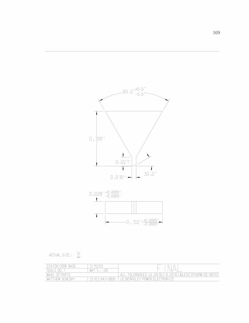
169

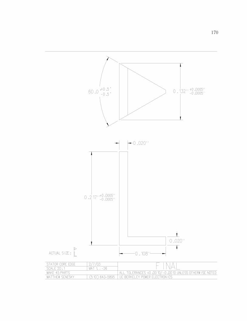
170

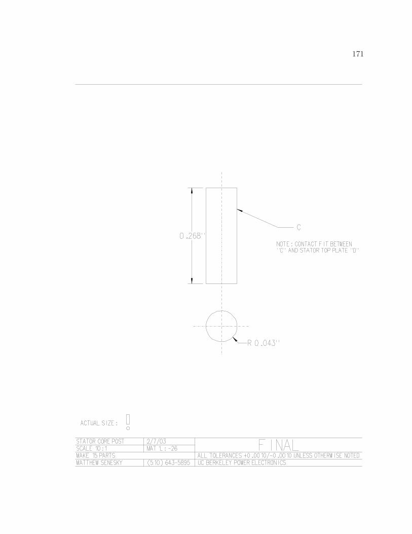
171

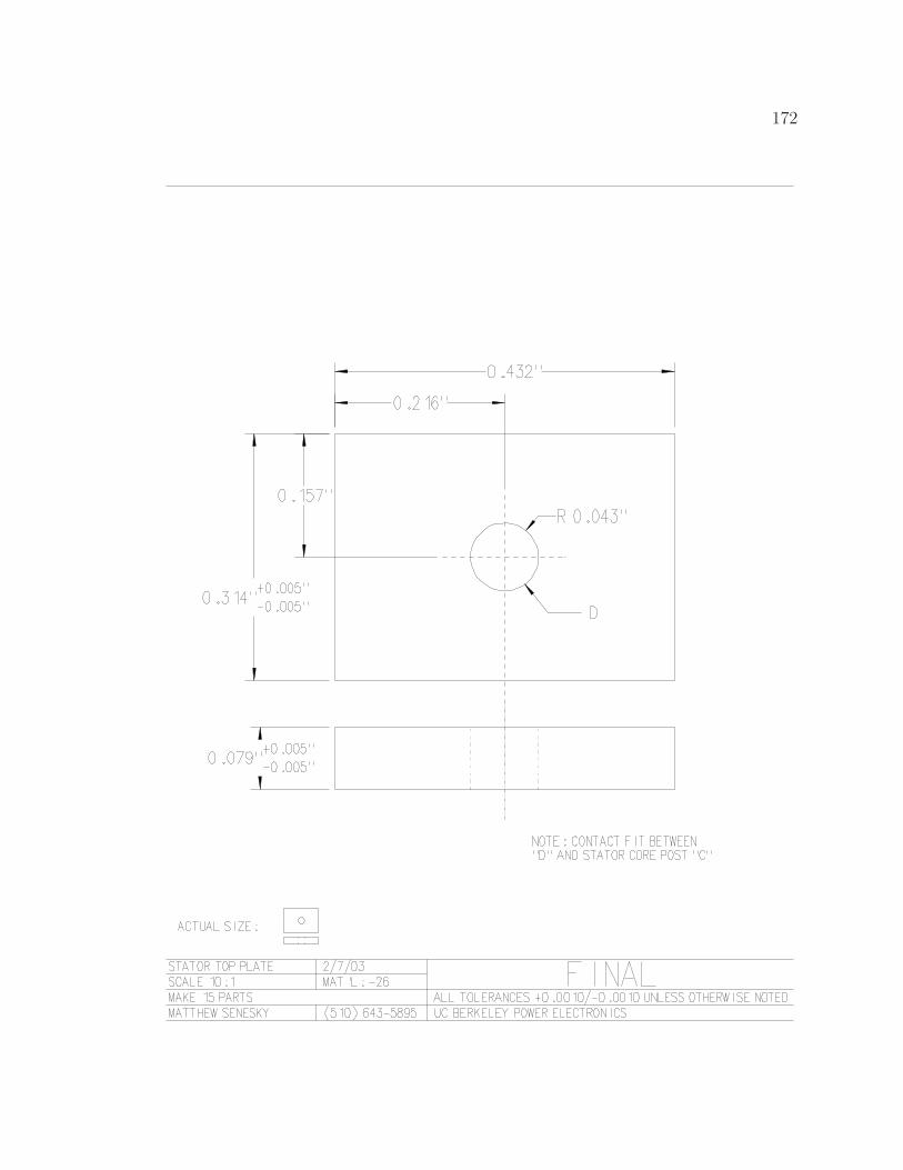
172

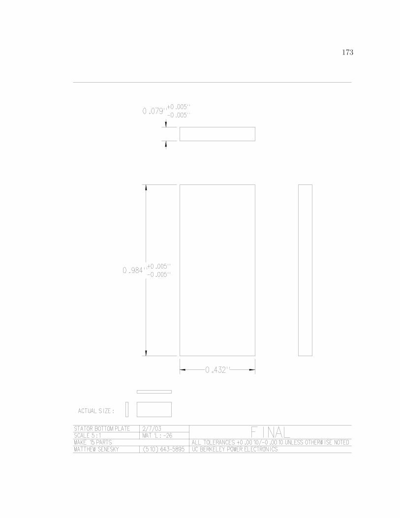
173

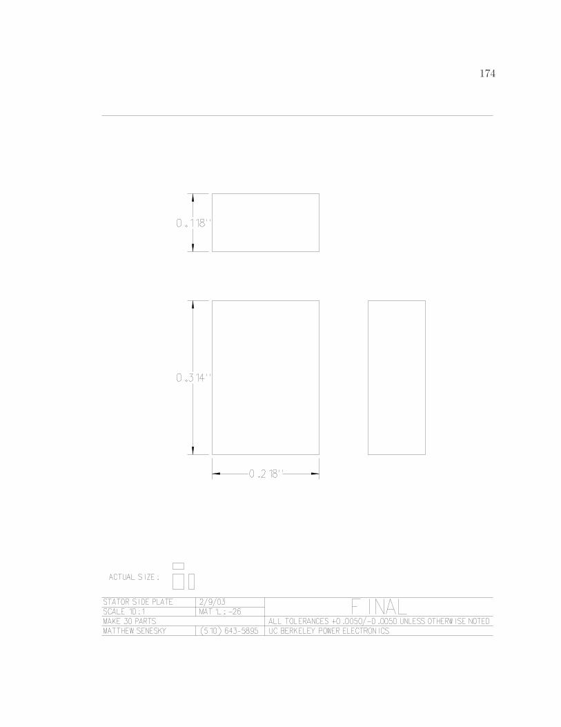
174

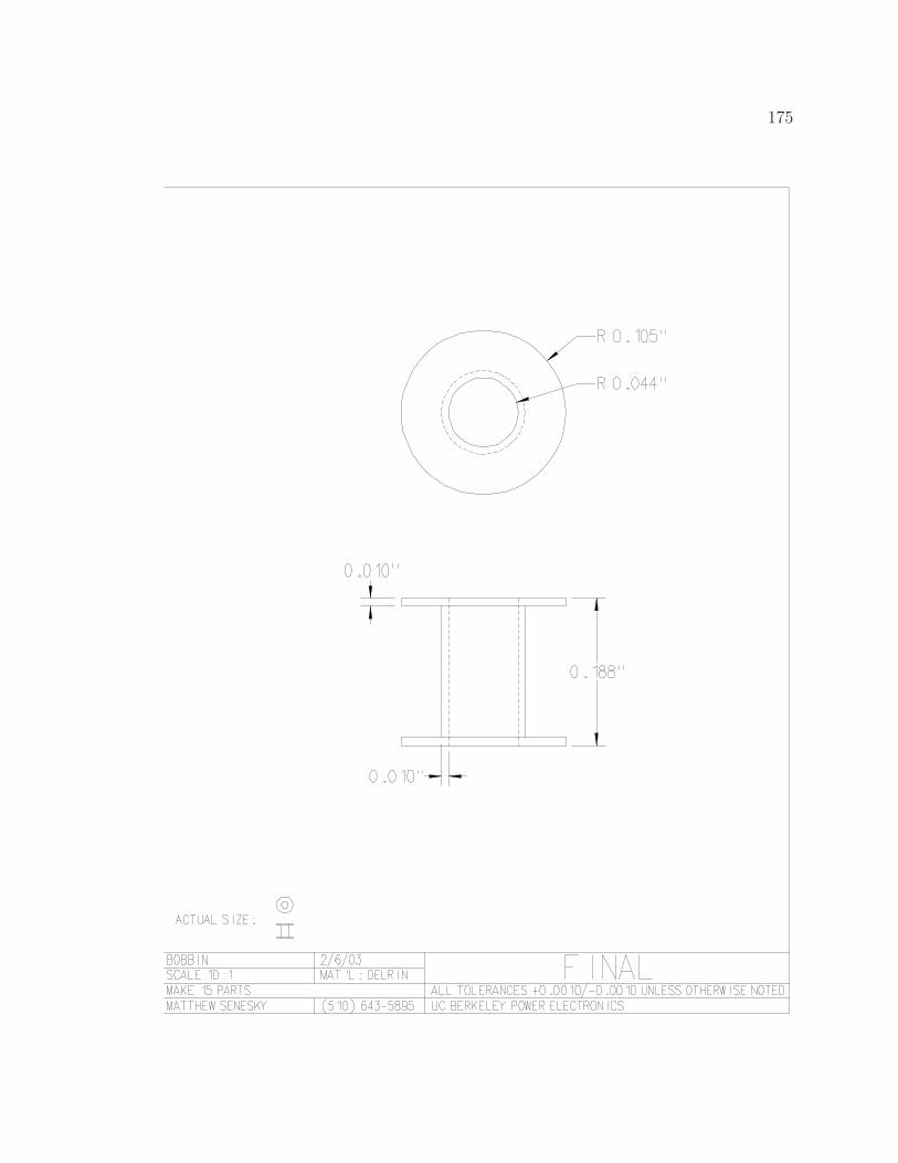
175