Electromagnetic Field Theory (EMT)nanotechlab.itu.edu.pk/wp-content/uploads/2017/01/Lectrure-1-and-2.pdf · force, electric field intensity …). EM theory is essentially a study

Instructor: Dr. M. Qasim Mehmood (PhD, NUS)

Teaching Assistants:

1) Humza Riaz (MS in Computer Science, ITU)

2) Qazi Salman Ahmed (M.Phil Physics, GCU)

Electromagnetic Field Theory (EMT)

Lecture # 1 + 2

Course Introducing & Vector Algebra

Prerequisite for EMT:

Electricity and Magnetism Electricity:

1) Electric Charge and Electric Field.

2) Gauss's Law & its Applications.

3) Electric Potential.

4) Capacitors and Dielectrics.

5) Current, Resistance, and DC Circuits.

Magnetism:

1) Magnetic Field and Magnetic Force.

2) Sources of Magnetic Fields.

3) Electromagnetic Induction.

4) Magnetic Properties of Materials.

5) Inductance

6) Alternating Current

Course Outlines of EMT:

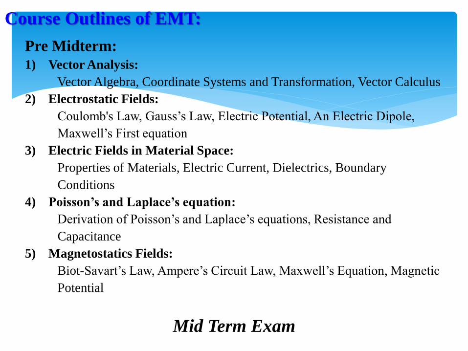
Pre Midterm:

1) Vector Analysis:

Vector Algebra, Coordinate Systems and Transformation, Vector Calculus

2) Electrostatic Fields:

Coulomb's Law, Gauss’s Law, Electric Potential, An Electric Dipole,

Maxwell’s First equation

3) Electric Fields in Material Space:

Properties of Materials, Electric Current, Dielectrics, Boundary

Conditions

4) Poisson’s and Laplace’s equation:

Derivation of Poisson’s and Laplace’s equations, Resistance and

Capacitance

5) Magnetostatics Fields:

Biot-Savart’s Law, Ampere’s Circuit Law, Maxwell’s Equation, Magnetic

Potential

Mid Term Exam

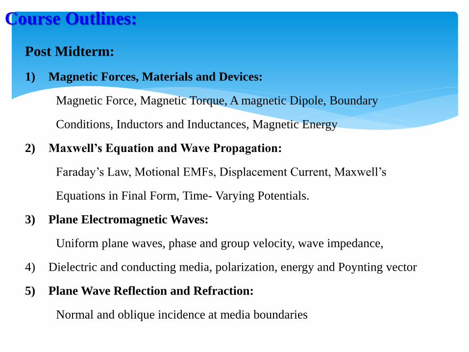
Course Outlines:

Post Midterm:

1) Magnetic Forces, Materials and Devices:

Magnetic Force, Magnetic Torque, A magnetic Dipole, Boundary

Conditions, Inductors and Inductances, Magnetic Energy

2) Maxwell’s Equation and Wave Propagation:

Faraday’s Law, Motional EMFs, Displacement Current, Maxwell’s

Equations in Final Form, Time- Varying Potentials.

3) Plane Electromagnetic Waves:

Uniform plane waves, phase and group velocity, wave impedance,

4) Dielectric and conducting media, polarization, energy and Poynting vector

5) Plane Wave Reflection and Refraction:

Normal and oblique incidence at media boundaries

Recommended Books & Grading Policy:

Books:

1) Elements of Electromagnetics by Matthew N. O Sadiku .

2) Fundamentals of Electromagnetics with Matlab by Karl E. Lonngren, Sava

V. Savov and Randy J. Jost

3) Engineering Electromagnetics William H. Hayt, Jr. John A. Buck

Attendance

1) Lecturers are very important

2) Less than 75 % (won’t be allowed for exam)

Grading Policy

1) Surprise Quizzes (3 %)

2) Five Quizzes (12 %)

3) Five Assignments (10 %)

4) Mid Term Exam (25 %)

5) Final Exam (50 %)

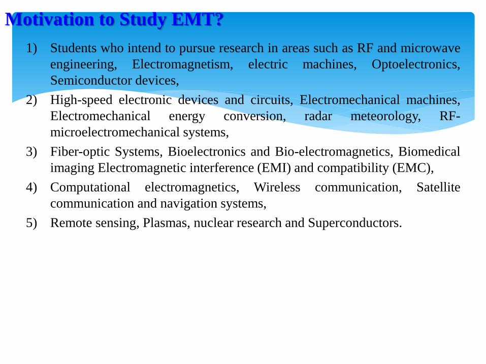
Motivation to Study EMT?

1) Students who intend to pursue research in areas such as RF and microwave

engineering, Electromagnetism, electric machines, Optoelectronics,

Semiconductor devices,

2) High-speed electronic devices and circuits, Electromechanical machines,

Electromechanical energy conversion, radar meteorology, RF-

microelectromechanical systems,

3) Fiber-optic Systems, Bioelectronics and Bio-electromagnetics, Biomedical

imaging Electromagnetic interference (EMI) and compatibility (EMC),

4) Computational electromagnetics, Wireless communication, Satellite

communication and navigation systems,

5) Remote sensing, Plasmas, nuclear research and Superconductors.

Applications of EMT?

1) Video to Show

2) EM principles find applications in various allied disciplines such as

microwaves, antennas, electric machines, satellite communications, bio-

electromagnetics, plasmas, nuclear research, fiber optics,

3) Electromagnetic interference and compatibility, electromechanical energy

conversion, radar meteorology," and remote sensing.

Note to Students:

1) The course of Electromagnetic Filed Theory including Antennas and wave

propagation is generally regarded by most students as one of the most

difficult courses in physics or the electrical engineering curriculum.

2) But this misconception may be proved wrong if you take following

precautions

a) Pay particular attention to Vector Analysis and Integro-differential

Calculus, the mathematical tool for this domain.

b) Do not attempt to memorize too many formulas. Memorize only the

basic ones, which are usually boxed, and try to derive others from

these. Try to understand how formulas are related.

c) Obviously, there is nothing like a general formula for solving all

problems. Each formula has some limitations due to the assumptions

made in obtaining it. Be aware of those assumptions and use the

formula accordingly.

d) Attempt to solve as many problems as you can. Practice is the best

way to gain skill.

Electromagnetics (EM) is a branch of physics or electrical engineering

in which electric and magnetic phenomena are studied.

EM may be regarded as the study of the interactions between electric

charges at rest and in motion.

Electromagnetics

EM principles find applications in various disciplines such as

microwaves, antennas, electric machines, satellite communications, fibre

optics, electromagnetic interference and compatibility ….

Electromagnetics

Vector analysis is a mathematical tool with which EM concepts are

most conveniently expressed and comprehended.

A scalar is a quantity that has only magnitude (time, mass, distance ....)

A vector is a quantity that has both magnitude and direction (velocity,

force, electric field intensity …).

EM theory is essentially a study of some particular fields.

A field can be scalar or vector and is a function that specifies a

particular quantity everywhere in a region

Examples of scalar fields are temperature distribution in a building,

electric potential in a region …

The gravitational force on a body in space is an example of vector field

Scalars and Vectors

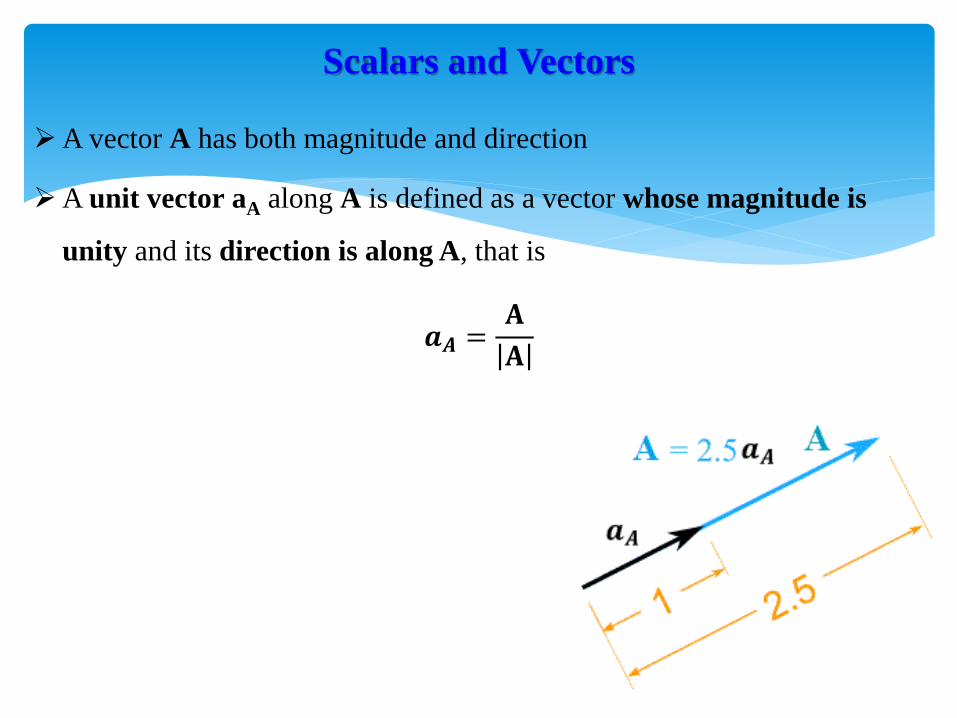
A vector A has both magnitude and direction

A unit vector aA along A is defined as a vector whose magnitude is

unity and its direction is along A, that is

𝒂𝑨 =𝐀

𝐀

Scalars and Vectors

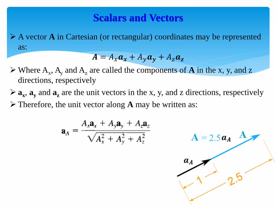
A vector A in Cartesian (or rectangular) coordinates may be represented

as:

𝑨 = 𝐴𝑥𝒂𝒙 + 𝐴𝑦𝒂𝒚 + 𝐴𝑧𝒂𝒛

Where Ax, Ay and Az are called the components of A in the x, y, and z

directions, respectively

ax, ay and az are the unit vectors in the x, y, and z directions, respectively

Therefore, the unit vector along A may be written as:

Scalars and Vectors

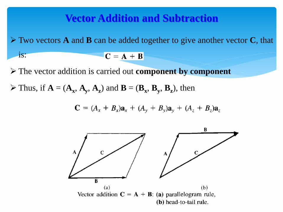
Two vectors A and B can be added together to give another vector C, that

is:

The vector addition is carried out component by component

Thus, if A = (Ax, Ay, Az) and B = (Bx, By, Bz), then

Vector Addition and Subtraction

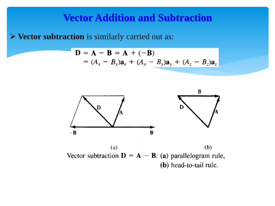
Vector subtraction is similarly carried out as:


The three basic laws of algebra obeyed by any given vectors A, B, and

C, are summarized as follows:


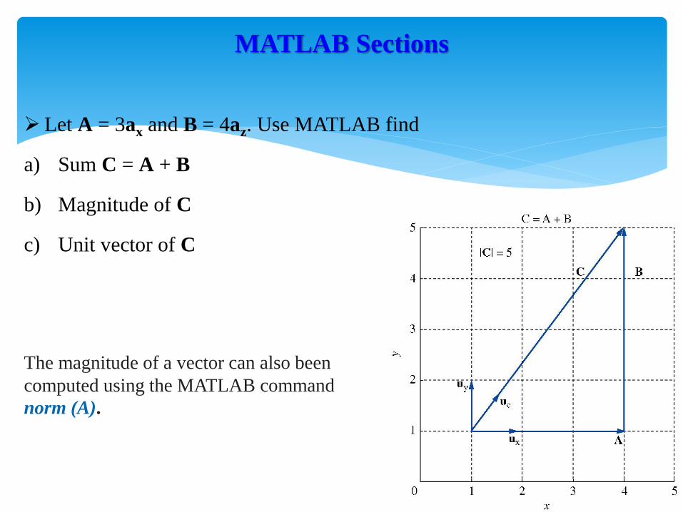
Let A = 3ax and B = 4az. Use MATLAB find

a) Sum C = A + B

b) Magnitude of C

c) Unit vector of C

MATLAB Sections

The magnitude of a vector can also been

computed using the MATLAB command

norm (A).

Point P in Cartesian coordinates may be represented by (x, y, z)

The position vector rp (or radius vector) of point P is defined as the

directed distance from the origin O to P, i.e.

Position Vector

For point (3, 4, 5), the position vector

is shown in the figure

𝒓𝑷 = 𝑂𝑃 = 𝑥𝒂𝒙 + 𝑦𝒂𝒚 + 𝑧𝒂𝒛

The distance vector is the displacement from one point to another

For two points P and Q given by (xP, yP, zp) and (xQ, yQ, zQ), the distance

vector (or separation vector) is the displacement from P to Q, that is:

Distance Vector

𝒓𝑷𝑸 = 𝒓𝑸 − 𝒓𝑷 = 𝑥𝑄 − 𝑥𝑃 𝒂𝒙 + 𝑦𝑄 − 𝑦𝑃 𝒂𝒚 + 𝑧𝑄 − 𝑧𝑃 𝒂𝒛

A vector field is said to be constant or uniform if it does not depend on

space variables x, y, and z.

For example, vector B = 3ax — 2ay + 10az is a uniform vector while

vector A = 2xyax + y2ay — xz2az is not uniform

Distance Vector

1) Scalar (or dot) product: 𝑨 ∙ 𝑩

2) Vector (or cross) product: 𝑨 × 𝑩

Multiplication of three vectors A, B, and C can result in either:

3) Scalar triple product: 𝑨 ∙ 𝑩 × 𝑪 ,

4) Vector triple product: 𝑨 × 𝑩 × 𝑪 ,

Vector Multiplication

The dot product of A and B is the length of the projection of A onto B multiplied by the

length of B.

Dot product could be viewed as "how much a vector is parallel to another vector",

The dot product of two vectors A and B, written as A • B, is defined geometrically as the

product of the magnitudes of A and B and the cosine of the angle between them

Also called scalar product: 𝑨 ∙ 𝑩 = 𝐴𝐵 cos 𝜃

𝑝𝑟𝑜𝑗𝐵𝑨 = 𝑨 cos 𝜃 = 𝑨 ∙ 𝑩 |𝑩| =𝑨∙𝑩

|𝑩|2𝑩,

𝑝𝑟𝑜𝑗𝐴𝑩 = 𝑩 cos 𝜃 = 𝑨 ∙ 𝑩 |𝑨| =𝑨∙𝑩

|𝑨|2𝑨

Vector Multiplication – Dot Product

For example, if we are to move a box a distance ∆x in a prescribed direction, we must

apply a certain force ‘F’ in the same direction. The total work W is given by the compact

expression

∆𝑊 = 𝑭 ∙ ∆𝒙


Other Examples:

1) Electric Flux

2) Magnetic Flux

𝒅𝝋𝑩 = 𝐵⊥𝑑𝐴 = 𝐵 cos𝜑 𝑑𝐴 = 𝑩 ∙ 𝑨


Algebraically, If A = (Ax, Ay, Az) and B = (Bx, By, Bz), then

Note that:


The MATLAB command that permits taking a scalar product of the two

vectors A and B is dot (A, B) or dot (B, A).


Area of Parallelogram:

𝐀𝐫𝐞𝐚 = 𝑩𝒂𝒔𝒆 × 𝑯𝒆𝒊𝒈𝒉𝒕 = 𝐶𝐵𝑠𝑛

Vector Multiplication – Cross Product

Parallelepiped:

Consists of six parallelograms

The cross product could be viewed "how much a vector is perpendicular to

another vector"

The cross product of two vectors A and B, written as A x B, is a vector quantity

whose magnitude is the area of the parallelopiped formed by A and B and is in the

direction of the right thumb when the fingers of the right hand rotate from A to B

where ‘an’ is a unit vector normal to the plane containing A and B


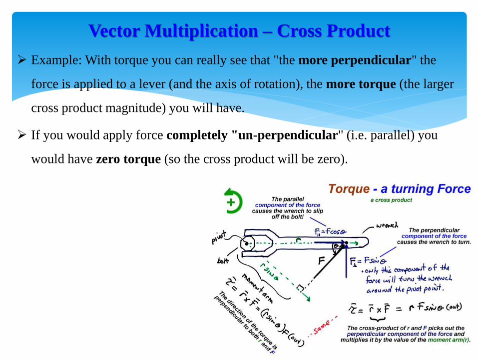
Example: With torque you can really see that "the more perpendicular" the

force is applied to a lever (and the axis of rotation), the more torque (the larger

cross product magnitude) you will have.

If you would apply force completely "un-perpendicular" (i.e. parallel) you

would have zero torque (so the cross product will be zero).


If A = (Ax, Ay, Az) and B = (Bx, By, Bz), then

Note that:


The MATLAB command that summons the vector product of two vectors A

and B is cross(A, B).


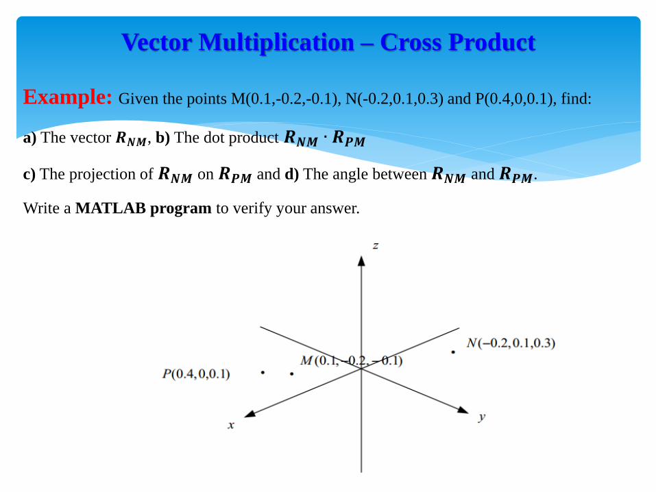
Example: Given the points M(0.1,-0.2,-0.1), N(-0.2,0.1,0.3) and P(0.4,0,0.1), find:

a) The vector 𝑹𝑵𝑴, b) The dot product 𝑹𝑵𝑴 ∙ 𝑹𝑷𝑴

c) The projection of 𝑹𝑵𝑴 on 𝑹𝑷𝑴 and d) The angle between 𝑹𝑵𝑴 and 𝑹𝑷𝑴.

Write a MATLAB program to verify your answer.


Assignment: Given the vectors R1 = ax + 2ay + 3az, R2 = 3ax + 2ay + az. Find a)

the dot product R1 . R2 , b) the projection of R1 on R2 , c) the angle between R1

and R2. Write a MATLAB program to verify your


Given three vectors A, B, and C, we define the scalar triple product as

𝑨 ∙ 𝑩 × 𝑪 = 𝑩 ∙ 𝑪 × 𝑨 =𝑪 ∙ 𝑨 × 𝑩

If A = (Ax, Ay, Az), A = (Bx, By, Bz), and C = (Cx, Cy, Cz), then 𝑨 ∙ 𝑩 × 𝑪 is the

volume of a parallelepiped having A, B, and C as edges and is easily obtained by

finding the determinant of the 3 X 3 matrix formed by A, B, and C;

𝑨 ∙ 𝑩 × 𝑪 =

𝐴𝑥 𝐴𝑦 𝐴𝑧𝐵𝑥 𝐵𝑦 𝐵𝑧𝐶𝑥 𝐶𝑦 𝐶𝑧

Since the result of this vector multiplication is scalar, hence is called the scalar triple

product.

Vector Multiplication – Scalar Triple Product

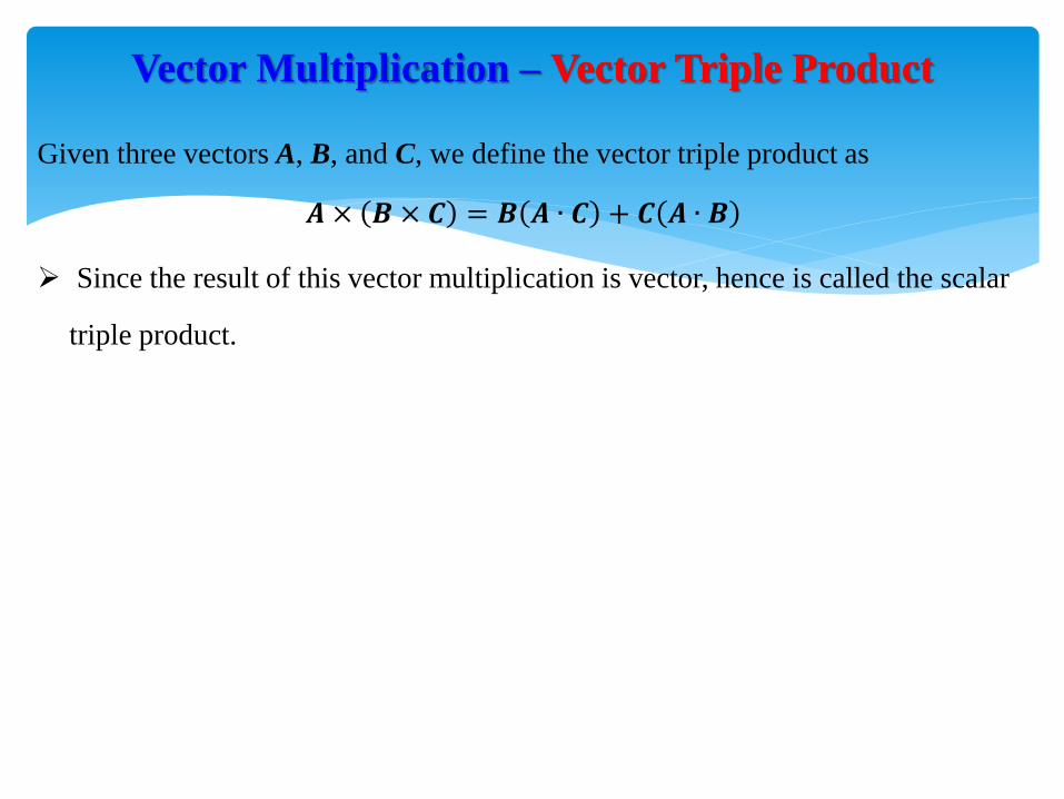
Given three vectors A, B, and C, we define the vector triple product as

𝑨 × 𝑩 × 𝑪 = 𝑩 𝑨 ∙ 𝑪 + 𝑪 𝑨 ∙ 𝑩

Since the result of this vector multiplication is vector, hence is called the scalar

triple product.

Vector Multiplication – Vector Triple Product

Documents

Electromagnetic Field Theory (EMT)nanotechlab.itu.edu.pk/wp-content/uploads/2017/01/Lectrure-1-and-2.pdf · force, electric field intensity …). EM theory is essentially a study