Electromagnetic Field Theory (EMT)

Lecture # 25

1) Transformer and Motional EMFs

2) Displacement Current

3) Electromagnetic Wave Propagation

Waves

&

Applications

Time Varying FieldsUntil now, we have restricted our discussions to static, or time invariant

Electric and Magnetic fields

Next, we shall examine situations where electric and magnetic fields aredynamic, or time varying

It should be mentioned first that in static EM fields, electric andmagnetic fields are independent of each other

Whereas in dynamic EM fields, the two fields are interdependent

In other words, a time-varying electric field necessarily involves acorresponding time-varying magnetic field

Time Varying Fields

Time-varying EM fields, represented by E(x, y, z, t) and H(x, y, z, t), are

of more practical value than static EM fields

Time-varying fields or waves are usually due to accelerated charges or

time-varying currents such as sine or square waves

Any pulsating current will produce radiation (time-varying fields)

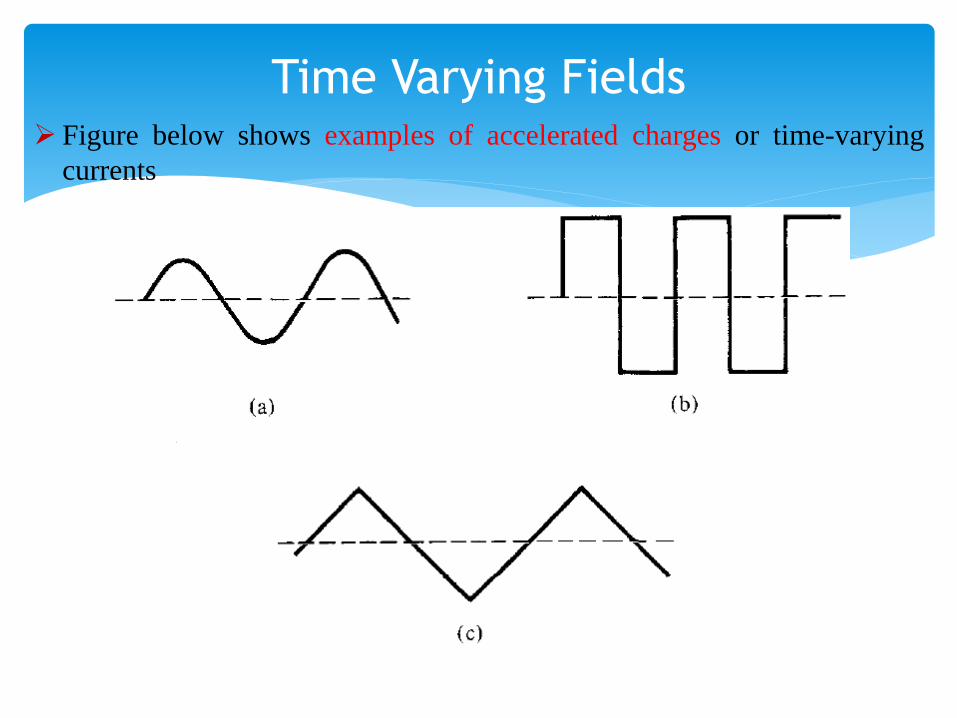
Time Varying Fields Figure below shows examples of accelerated charges or time-varying

currents

Time Varying Fields

In summary:

Stationary charges →Electrostatic fields

Steady currents → Magneto-static fields

Time-varying currents → electromagnetic fields (or waves)

Electromagnetic Field Theory (EMT)

Lecture # 24

1) Magnetic Torque and Momentum

2) Inductance and Magnetic Energy

3) Introduction to Time Varying Fields

4) Faraday’s Law

Faraday’s LawAfter Oersted's experimental discovery (upon which Biot-Savart and

Ampere based their laws) that a steady current produces a magnetic field,

it seemed logical to find out if magnetism would produce electricity.

In 1831, about 11 years after Oersted's discovery, Michael Faraday in

London and Joseph Henry in New York discovered that a time-varying

magnetic field would produce an electric current.

According to Faraday's experiments, a static magnetic field produces no

current flow, but a time-varying field produces an induced voltage

(called electromotive force or simply emf) in a closed circuit, which

causes a flow of current

Induction Experiments:

But when we move the magnet either toward or away from the coil, the

meter shows current in the circuit (Fig. b).

If we keep the magnet stationary and move the coil, we again detect a

current during the motion.

We call this an induced current, and the corresponding emf required to cause

this current is called an induced emf.

Faraday’s Law The Faraday’s law states that the induced emf, Vemf (in volts), in any

closed circuit is equal to the time rate of change of the magnetic flux

linkage by the circuit

Mathematically, Faraday’s law can be expressed as:

where N is the number of turns in the circuit and Ψ is the flux through

each turn

Lenz's law states that the direction of current flow in the circuit is such

that the induced magnetic field produced by the induced current will

oppose the original magnetic field.

Faraday’s Law From Lenz’s law, the negative sign shows that the induced voltage acts in

such a way as to oppose the flux producing it

Recall that we described an electric field as one in which electric charges

experience force.

The electric fields considered so far are caused by electric charges; in

such fields, the flux lines begin and end on the charges

There are other kinds of electric fields not directly caused by electric

charges

These are emf-produced fields

Faraday’s Law The Faraday’s law states that the induced emf, Vemf (in volts), in any

closed circuit is equal to the time rate of change of the magnetic flux

linkage by the circuit

Mathematically, Faraday’s law can be expressed as:

where N is the number of turns in the circuit and Ψ is the flux through

each turn

Lenz's law states that the direction of current flow in the circuit is such

that the induced magnetic field produced by the induced current will

oppose the original magnetic field.

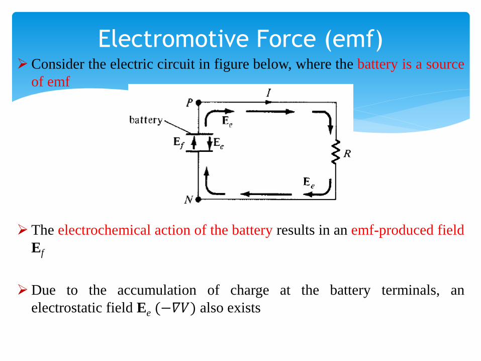
Electromotive Force (emf)Consider the electric circuit in figure below, where the battery is a source

of emf

The electrochemical action of the battery results in an emf-produced field

Ef

Due to the accumulation of charge at the battery terminals, an

electrostatic field Ee (−𝛻𝑉) also exists

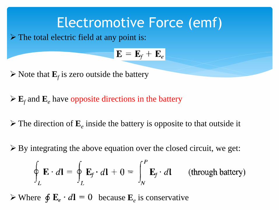
Electromotive Force (emf) The total electric field at any point is:

Note that Ef is zero outside the battery

Ef and Ee have opposite directions in the battery

The direction of Ee inside the battery is opposite to that outside it

By integrating the above equation over the closed circuit, we get:

Where because Ee is conservative

Electromotive Force (emf) The emf of the battery is the line integral of the emf-produced field, that

is:

The negative sign is because Ef and Ee are equal but opposite within the

battery

It is important to note that:

An electrostatic field Ee cannot maintain a steady current in a closed

circuit since

An emf-produced field Ef is non-conservative.

Transformer and Motional EMFsAfter considering the connection between emf and electric field, we now

examine how Faraday's law links electric and magnetic fields

For a circuit with a single turn (N = 1), we have:

In terms of E and B, the above equation may be written as:

where Ψ has been replaced by and S is the surface area of the

circuit bounded by the closed path L

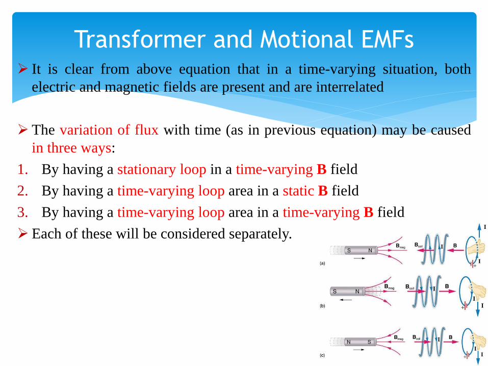
Transformer and Motional EMFs It is clear from above equation that in a time-varying situation, both

electric and magnetic fields are present and are interrelated

The variation of flux with time (as in previous equation) may be caused

in three ways:

1. By having a stationary loop in a time-varying B field

2. By having a time-varying loop area in a static B field

3. By having a time-varying loop area in a time-varying B field

Each of these will be considered separately.

Stationary Loop; Time-Varying B Field Figure below shows a stationary conducting loop in a time varying

magnetic B field

The emf is given as:

This emf induced by the time-varying B field in a stationary loop is often

referred to as transformer emf in power analysis since it is due to

transformer action

Observe in the figure that the Lenz's law is

obeyed; the induced current I flows such

as to produce a magnetic field that

opposes B(t)

Stationary Loop; Time-Varying B Field

By applying Stokes theorem to the emf equation, we obtain:

Therefore, we get:

This is one of the Maxwell's equations for time-varying fields

It shows that the time varying E field is not conservative

This implies that the work done in taking a charge about a closed path in

a time-varying electric field, for example, is due to the energy from the

time-varying magnetic field

Moving Loop; Static B Field

When a conducting loop is moving in a static B field, an emf is induced

in the loop

Recall that the force on a charge moving with uniform velocity u in a

magnetic field B is:

We define the motional electric field Em as:

If we consider a conducting loop, moving with uniform velocity u as

consisting of a large number of free electrons, the emf induced in the

loop is:

Moving Loop; Static B Field

This type of emf is called motional emf or flux-cutting emf because it is

due to motional action

It is the kind of emf found in electrical machines such as motors,

generators, and alternators.

Moving Loop; Time varying B Field

In this case, both transformer emf and motional emf are present

Hence we combine both the emfs as:

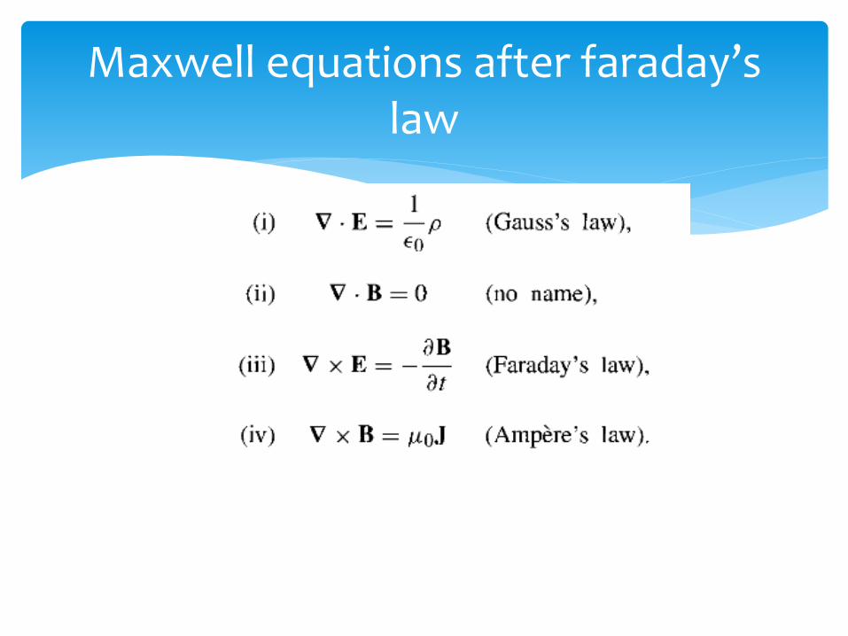
Maxwell equations after faraday’s law

Electromagnetic Field Theory (EMT)

Lecture # 25

1) Transformer and Motional EMFs

2) Displacement Current

3) Electromagnetic Wave Propagation

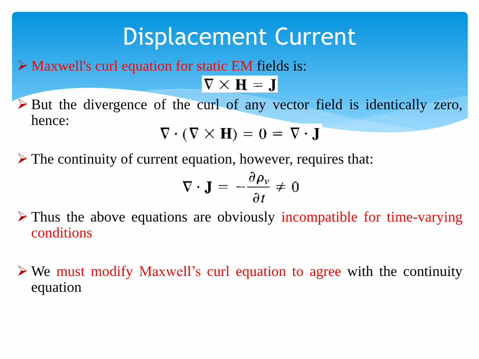
Displacement CurrentMaxwell's curl equation for static EM fields is:

But the divergence of the curl of any vector field is identically zero,hence:

The continuity of current equation, however, requires that:

Thus the above equations are obviously incompatible for time-varyingconditions

We must modify Maxwell’s curl equation to agree with the continuityequation

Displacement Current To do this, we add a term to Maxwell’s curl equation so that it becomes:

where Jd is to be determined and defined

Again, the divergence of the curl of any vector is zero, hence:

In order for the above equation to agree with the continuity equation:

Or:

Displacement Current Substituting Jd into Maxwell’s curl equation, we get:

This is Maxwell's equation (based on Ampere's circuit law) for a time-

varying field

The term Jd is known as displacement current density and J is the

conduction current density

The insertion of Jd into Maxwell’s curl equations was one of the major

contributions of Maxwell

Without the term Jd, electromagnetic wave propagation (radio or TV

waves, for example) would be impossible

Displacement Current

At low frequencies, Jd is usually neglected compared with J, however, at

radio frequencies, the two terms are comparable

At the time of Maxwell, high-frequency sources were not available and

the curl equation could not be verified experimentally

It was years later that Hertz succeeded in generating and detecting radio

waves thereby verifying the curl equation

This is one of the rare situations where mathematical argument paved the

way for experimental investigation.

Displacement Current

Based on the displacement current density, we define the displacement

current as:

It must be kept in mind that displacement current is a result of time-

varying electric field

A typical example of such current is the current through a capacitor when

an alternating voltage source is applied to its plates

Maxwell’s Equations For a field to be "qualified" as an electromagnetic field, it must

satisfy all four Maxwell's equations

Problem-1

In free space, E = 20 cos (wt - 50x) ay V/m. Calculate

(a) Jd

(b) H

(c) w