Embed Size (px)
Citation preview

Electric Vehicle Charging Impact on Load Profile
PIA GRAHN
Licentiate Thesis
Stockholm, Sweden 2013

TRITA-EE 2012:065ISSN 1653-5146ISBN 978-91-7501-592-7
School of Electrical EngineergingRoyal Institute of Technology
SE-100 44 StockholmSWEDEN
Akademisk avhandling som med tillstånd av Kungl Tekniska högskolan framläggestill offentlig granskning för avläggande av Teknologie licentiatexamen i elektrotekniskasystem torsdagen den 17 januari 2013 klockan 10.00 i i sal E3, Kungliga TekniskaHögskolan, Osquars backe 14, Stockholm.
© Pia Grahn, January 2013
Tryck: Eprint AB 2012
iii
Abstract
One barrier to sustainable development is considered to be greenhousegas emissions and pollution caused by transport, why climate targets are setaround the globe to reduce these emissions. Electric vehicles (EVs), may bea sustainable alternative to internal combustion engine vehicles since havingEVs in the car park creates an opportunity to reduce greenhouse gas emissions.This is due to the efficiency of the electric motor. For EVs with rechargeablebatteries the opportunity to reduce emissions is also dependent on the genera-tion mix in the power system. EVs with the possibility to recharge the batteryfrom the power grid are denoted plug-in electric vehicles (PEVs) or plug-in-hybrid electric vehicles (PHEVs). Hybrid electric vehicles (HEVs), withoutexternal recharging possibility, are not studied, hence the abbreviation EVfurther covers PHEV and PEV.
With an electricity-driven private vehicle fleet, the power system will ex-perience an increased amount of variable electricity consumption that is de-pendent on the charging patterns of EVs. Depending on the penetration levelof EVs and the charging patterns, EV integration creates new quantities inthe overall load profile that may increase the load peaks. The charging pat-terns are stochastic since they are affected by the travel behavior of the driverand the charging opportunities which imply that the EV integration also willhave an effect on the load variations. Increased load variation and load peaksmay create a need for upgrades in the grid infrastructure to reduce the riskfor losses, overloads or damaging of components. However, with well-designedincentives to the EV users the variable electricity consumption due to electricvehicle charging (EVC) may become a flexible load that can help the powersystem mitigate load variations and load peaks.
The aim with this licentiate thesis is to investigate the impact of EVCon load profiles and load variations. The thesis reviews and categorizes EVCmodels in previous research. The thesis furthermore develops electric vehiclecharging models to estimate the charging impact based on charging patternsinduced by private car travel behavior. The models mainly consider uncon-trolled charging (UCC) related to stochastic individual car travel behaviorand induced charging needs for PHEVs. Moreover, the thesis comments onthe potential of individual charging strategies (ICS) with flexible chargingand external charging strategies (ECS).
Three key factors are identified when considering the impact of EVC onload profiles and load variations. The key factors are: The charging moment,the charging need and the charging location. It is concluded that the level ofdetails concerning the approach to model these key factors in EVC models willimpact the estimations of the load profiles. This means that models takinginto account a higher level of mobility details will be able to create a morerealistic estimation of a future UCC behavior, enabling for more accurateestimates of the impact on load profiles and the potential of ICS and ECS.
iv
Sammanfattning
Utsläpp av växthusgaser och andra föroreningar orsakade av transportsek-torn kan anses vara en barriär för en hållbar utveckling. För att minska dessautsläpp har flertalet klimatmål satts upp världen över. Med en introduktionav elbilar i bilparken skapas en möjlighet att minska utsläppen eftersom elbi-lar kan vara ett hållbart alternativ till bilar med förbränningsmotor tack vareden höga verkningsgraden hos elmotorn. För elbilar med uppladdningsbarabatterier så är möjligheten att minska utsläpp också beroende av produktion-smixen i elsystemet. I denna avhandling så studeras elbilar med uppladdnings-bara batterier.
I en framtid med en bilpark bestående av en stor andel elbilar kommerelsystemet att uppleva en ökad mängd varierande elkonsumtion beroendepå elbilarnas laddningsmönster. Elbilars laddning påverkar lastprofilen ochberoende på mängden elbilar i systemet kan lasttoppar och lastvariationerkomma att öka. Laddningsmönstren är stokastiska eftersom de påverkas avbilförares resvanor och laddningsmöjligheter och detta medför också att last-variationerna kommer att påverkas. Om variationen i lasten ökar så kan dettabetyda att nya investeringar i elnätets infrastruktur blir nödvändiga för attminska risken för förluster, överbelastningar och skada av komponenter i el-nätet. Med väldesignade incitament för elbilsanvändare har den varierandeelbilslasten istället potentialen att bli en flexibel last som kan användas föratt minska lastvariationer och lasttoppar.
Syftet med denna licentiatavhandling är att undersöka påverkan på last-profiler och lastvariationer på grund av elbilsladdning. I avhandlingen utförsen litteraturstudie och en kategorisering av befintliga elbilsladdningsmodeller.Dessutom introduceras nya elbilsladdningsmodeller med vilka man kan upp-skatta laddningsmönster utifrån körvanor och undersöka uppkomna laddnings-mönsters påverkan på lastprofiler. Modellerna beaktar i huvudsak okontroller-ad laddning som baseras på stokastiskt individuellt körmönster och därmedorsakade laddningsbehov för elbilar. Avhandlingen diskuterar också poten-tialen av laddningsstrategier baserade på priskänslighet hos flexibla individereller baserade på extern laddningsstyrning.
Tre nyckelfaktorer vid elbilsladdningsmodellering är identifierade när detgäller påverkan på lastprofiler och lastvariationer. Nyckelfaktorerna är: ladd-
ningstillfället, laddningsbehovet och laddningsplatsen. En av avhandlingensslutsatser är att detaljnivån i ansatsen när man modellerar dessa nyckelfak-torer har en signifikant påverkan på uppskattningarna av lastprofilerna. Det-ta innebär att modeller som beaktar en högre detaljnivå hos elbilsanvändningkommer att ge mer realistiska uppskattningar av ett framtida laddningsmön-ster. Detta betyder även en högre noggrannhet hos uppskattningarna av po-tentialen för laddningsstrategier baserade på priskänslighet hos flexibla indi-vider och även laddningsstrategier baserade på extern kontroll.

ACKNOWLEDGEMENTS v
Acknowledgements
This thesis is part of a PhD project that started in June 2010 at the Division ofElectric Power Systems at the Royal Institute of Technology (KTH). I would liketo thank Lennart Söder for the intensive feedback, the ideas and for giving methe opportunity to write this thesis. Further, I am grateful to Karin Alvehag forthe comments on my work, the ideas of improvement and the great support. Iwould like to thank Joakim Munkhammar, Mattias Hellgren, Joakim Widén andJohanna Rosenlind for great co-operation and stimulating discussions. I would liketo acknowledge Trafikanalys for providing travel data from the RES0506 database.Moreover, the financial support from the Energy Systems Programme is acknowl-edged, and appreciation goes to the Buildings Energy Systems Consortium for theopportunity to share ideas across disciplines. I would also like to thank my col-leagues in the Energy Systems Programme and my colleagues at the division ofElectric Power Systems, all for their support, interesting discussions and sharedfika hours. Finally, gratitude goes to my family and friends for their love andemotional support.

Contents
Acknowledgements . . . . . . . . . . . . . . . . . . . . . . . . . . . . . . . v
Contents vi
1 Introduction 7
1.1 Background . . . . . . . . . . . . . . . . . . . . . . . . . . . . . . . . 71.2 Scientific objective . . . . . . . . . . . . . . . . . . . . . . . . . . . . 91.3 Contribution . . . . . . . . . . . . . . . . . . . . . . . . . . . . . . . 101.4 List of papers . . . . . . . . . . . . . . . . . . . . . . . . . . . . . . . 111.5 Division of work between authors . . . . . . . . . . . . . . . . . . . . 111.6 Outline . . . . . . . . . . . . . . . . . . . . . . . . . . . . . . . . . . 12
2 Previous research on electric vehicle integration 13
2.1 Electric vehicle charging opportunities . . . . . . . . . . . . . . . . . 132.2 Three key factors affecting EVC load profiles . . . . . . . . . . . . . 162.3 Conclusion of review . . . . . . . . . . . . . . . . . . . . . . . . . . . 19
3 Modeling electric vehicle charging 23
3.1 EVC-A: EVC to evaluate grid loading impact . . . . . . . . . . . . . 233.2 EVC-B: PHEV home-charging considering activity patterns . . . . . 263.3 EVC-C: PHEV mobility and recharging flexibility . . . . . . . . . . . 303.4 EVC-D: PHEV utilization considering type-of-trip and recharging
flexibility . . . . . . . . . . . . . . . . . . . . . . . . . . . . . . . . . 36
4 Case studies 47
4.1 Case study with the EVC-A model . . . . . . . . . . . . . . . . . . . 474.2 Case study with the EVC-B model . . . . . . . . . . . . . . . . . . . 544.3 Case study with the EVC-C model . . . . . . . . . . . . . . . . . . . 624.4 Case study with the EVC-D model . . . . . . . . . . . . . . . . . . . 684.5 Case study summary . . . . . . . . . . . . . . . . . . . . . . . . . . . 794.6 Concluding remarks . . . . . . . . . . . . . . . . . . . . . . . . . . . 82
5 Conclusion and future works 85
5.1 Concluding discussion . . . . . . . . . . . . . . . . . . . . . . . . . . 85
vi

CONTENTS vii
5.2 Future work . . . . . . . . . . . . . . . . . . . . . . . . . . . . . . . . 88
Bibliography 91


CONTENTS 1
Abbreviations
• EV, Electric vehicle
• PHEV, Plug-in-hybrid electric vehicle
• PEV, Plug-in electric vehicle
• SOC, State of charge
• DOD, Depth of discharge
• G2V, Grid-to-vehicle
• V2G, Vehicle-to-grid
• UCC, Uncontrolled charging
• UniC, Unidirectional charging
• BiC, Bidirectional charging
• ICS, Individual charging strategies
• ECS, External charging strategies
• DSO, Distribution system operator


Nomenclature
∆t Time step length [hr]
ηc, ηdc Charging efficiency, discharging efficiency
µ, ν States of electricity-dependent activities
τ Discrete time interval [0,...,T]
Qtµν , T t
m Transition matrices
{Xt; t ∈ τ} Stochastic process
Ai, Di Away period, driving period [mins]
At,ia Synthetic activity pattern
Bh Household consumption [kWh/(day and apartment)]
Ct,im Consumption level [kWh/h]
cm Electricity consumption in distance [kWh/km]
Cts Season coefficient
Ccost Total charging cost [e]
E = {1, ..., M} Set of states
Eisoc Electricity used [kWh]
Etp Charging price [e/kWh]
Ec, EF c Fixed charging cost, fixed fast charging cost [e]
Et,iC Electricity charging cost [e/kWh]
Et,id , Gt,i
d Distance driven with electricity, and with second fuel [km]
3

4 CONTENTS
Et,iE Electricity consumed from grid [kWh]
fp Percentage %
F imin Minimum state of charge fraction
gm Second fuel consumption in distance [liters/km]
Glc Second fuel price [e/liter]
Gt,iref Refill events [No.]
gt,iref ,nt,i
ch, nt,ifch Binary variables, 0 or 1
H Constant cost [e/kWh]
h, G, N, D, n, Ntot Constants
ki ∈ U(a, b), K ∈ U(0, 1) Random numbers
Li, T ci Leaving time, connecting time [min]
N , Eµ, M Number of activities, number of states, number of states [No.]
nch, nfch Charging events, fast charging events [No.]
ntDz Driving vehicles in state z [No.]
ntP x Parked vehicles in state x [No.]
ntP , nt
D Parked PHEVs, driving PHEVs [No.]
ntst,z, nt
en,z Starting type-of-trip, ending type-of-trip [No.]
ntx,tot, nt
z,tot Maximum type-of-trips x, z [No.]
P t,ih Household load [kW]
P t,iV EVC load [kW]
pt Electricity price [e/kWh]
P tn,h Normalized load
P ttot Total load [kW]
P tV tot Total EVC load [kW]

CONTENTS 5
Pc Charging power [kW]
pF Share of flexible chargers
P t,iL Charging price-limit [e/kWh]
ptµ,ν Transition probability
PA
t,ia
Load from electricity-dependent activities [kW]
pcar Vehicle usage probability
pdod Depth of discharge fraction
stw Standard deviation
St,i States
SOCt,i State of charge [kWh]
SOCimax Battery maximum storage [kWh]
SOT t,i State of tank [Liters]
SOT imax Tank maximum storage [Liters]
T Numbers of time steps
t, i, a, m Time step index, sample index, activity index, index
T iF Time period with charging prices above price-limit
vm Velocity [km/h]
x = {A, ..., NP } Parking states
Xt, W t,i Stochastic variables
z = {1, ..., ND} Driving states


Chapter 1
Introduction
1.1 Background
Climate targets around the world are set to reduce climate impacts suchas greenhouse gas emissions. The European Parliament has in a directiveidentified greenhouse gas emissions and pollution caused by transport as oneof the main obstacles to sustainable development [1]. The directive statesthat "the Commission continues with efforts to develop markets for energy-efficient vehicles through public procurements and awareness-raising". Ageneral concern is also the fact that fossil fuels are finite resources whichincreases the awareness of the dependence both on foreign oil producingcountries and oil as a resource. Electric vehicles (EVs) with the possibilityto recharge the battery from the power grid are denoted as plug-in elec-tric vehicles (PEVs) or plug-in-hybrid electric vehicles (PHEVs). PHEVsin addition to the electric motor also have the opportunity to use a sec-ond fuel, usually by an internal combustion engine. Hybrid electric vehicles(HEVs), without external recharging possibility, are not studied here, hencethe abbreviation EV further covers PHEV and PEV.
EVs are considered to be a sustainable alternative to the internal combus-tion engine vehicles since having EVs in the car park creates an opportunityto meet climate targets, by reducing greenhouse gas emissions such as CO2,and to reduce the transport sector’s dependency of fossil fuels. In for exam-ple Sweden, policies state that greenhouse gas emissions should be reducedwith 20-25% until 2020 and with 70-85% until 2050, and also that Swedenshould have a car park independent of fossil fuel by 2030 [2]. Measures toreach the targets are mentioned to be renewable fuels, more energy efficientvehicle techniques, hybrid vehicles and electric vehicles.
7
8 CHAPTER 1. INTRODUCTION
EVs are operated by efficient electricity motors with electricity from bat-teries which can be charged from the power grid. The energy source maythus be determined by the generation mix within the power system. Witha low rate of emissions in the power generation of the system the use ofEVs can reduce overall emissions within the transport sector. If the Swedishprivate car fleet of around 4.3 millions vehicles was electricity-driven, thenaround 5 · 109 liters of engine fuel, corresponding to around 45 TWh, couldbe exchanged into around 12 TWh electricity on a yearly basis [3]. Thiscorresponds to a yearly mean consumption of around 1370 MW. If all pri-vate cars in the world would be electricity-driven, they would consumearound 1200 TWh/year which is 5% of the total electricity consumptionof 23000 TWh in 2005 [4]. With an electricity-driven private vehicle fleet,the power system will experience an increased amount of variable electricityconsumption dependent on electric vehicle charging (EVC) patterns. Theseanticipated EVC patterns will create new quantities in the overall load pro-files and introduce new load variations. Vehicles are parked in average 90%of the time [5]. Assuming that the Swedish private car fleet was electricity-driven and 90% was connected to the grid for charging at the same moment,(230 V, 10 A), this would then correspond to a load increase of 8901 MW.In 2011 the Swedish demand varied between 8382 MW and 25363 MW [6].This means that EVC load may become significant and estimations of EVCpatterns and charging strategies are important.
With a change towards higher levels of EVs in the car park, the batteriesbecome a large and flexible capacity in the power system. This creates anopportunity for the EV batteries to act as individual and flexible loads whichmay become useful to consider for grid-support to mitigate load variationsand load peaks. If this capacity can be used it would be advantageous for theelectric system, especially when keeping the grid stable with an increasedamount of variable renewable energy. The opportunity of using EVs as gridancillary services was for example studied in [7–10]. If creating well-designedincentives for EV users to make the EV batteries take part in grid-support,the value of having an EV could be increased.
With EVs in the power system, the load profiles are related to the EVCpattern which is affected by the travel behavior of the EV user and theinduced charging need. The charging moment, the charging need and thecharging location, are in this thesis identified as key factors when consider-ing the impact of an EV introduction on the load profiles. If the Swedishprivate car fleet was electricity-driven and consuming in average 8 kWh/day,

1.2. SCIENTIFIC OBJECTIVE 9
(based on 0.2 kWh/km and 15000 km driven/year), this would mean a dailyelectricity use of 34 GWh, which is around 10% of the mean daily overallelectricity use. The time periods for this overall 10% consumption increasewould be decided by the EVC patterns. If it is possible to impact the EVCbehavior, these 12 TWh/year would correspond to an average flexible loadcapacity of around 1370 MW or more depending on the EVC patterns.
With a small number of vehicles, the power system might not be muchaffected by the charging. However, with a large number of vehicles, thecharacteristics of the charging patterns could have a significant impact onthe power system. This may result in overloading and power losses [11]. Thepeak load increase could become large especially with uncontrolled charging,(UCC) when each EV is charged individually related to travel behaviors andcharging needs. Hereby it becomes important to create and develop modelsrelated to the stochastic individual car travel behaviors and induced chargingneeds to be able to investigate and quantify the impact of a prospectiveintroduction of EVs.
1.2 Scientific objective
This thesis focuses on the overall possible impact of EVC on the load profilesand load variations. The purpose with the thesis is to create models of EVusage and induced EVC patterns. The thesis introduces EVC models thatcapture driving behavior variations and induced charging needs, and alsoEVC models that allow for charging flexibility. The EVC models focuses onthe underlying driving patterns and expected corresponding EVC profilesdue to charging need, charging location and charging moment. The EVCmodels allow for a quantification of the expected charging load as a functionof the introduction level of EVs in the vehicle fleet.
By using the models, it is possible to estimate time-dependent expectedcharging load profiles and load variation based on only home-charging orwith additional charging options. It is also possible to estimate the loadprofiles based on the type-of-trip and related charging opportunities, andalso with charging flexibility due to price sensitivity. Charging flexibilitydue to price sensitivity is defined as an individual charging strategy (ICS).By impacting the charging patterns with incentives, the models includingICS allow for available EV battery capacity to be used for example for valleyfilling.

10 CHAPTER 1. INTRODUCTION
1.3 Contribution
The licentiate thesis deals with EVC models of mainly UCC patterns in-duced by stochastic individual private car travel behavior and charging op-portunities, and also ICS with flexible charging due to price sensitivity. Thecontributions are:
• A literature review is made on integration of EVs. Previous researchis categorized based on assumptions in the EVC models regardingthe EVC opportunities; unidirectional charging (UniC), bidirectionalcharging (BiC), uncontrolled charging (UCC), external charging strate-gies (ECS) and individual charging strategies (ICS). A further groupingof previous research is also made based on identified key factors whenmodeling EVC. The grouping is based on three key factors: The charg-ing location, the charging need and the charging moment. The wholereview is presented in Chapter 2 and a part of it in paper I.
• Different charging scenarios are modeled (Model EVC-A) in paper IIto describe EVC load in order to investigate the impact of the EVintroduction level on grid components. The model is presented in sec-tion 3.1.
• A charging model (Model EVC-B) is developed in paper III with whichit is possible to estimate the load from PHEV home-charging relatedto the load from other electricity-dependent residential activities. Theresidential load profile, specified by the underlying activities includ-ing the EVC load, is the model output. The model is presented insection 3.2.
• A charging model (Model EVC-C) is developed in paper IV which cap-tures the stochastic individual driving behavior and charging opportu-nities related to each parking event. By using the model, it is possibleto estimate expected EVC load profiles as a function of time based onintroduction level and charging flexibility. The model is presented insection 3.3.
• A charging model (Model EVC-D) is developed in paper V which cap-tures different charging opportunities related to time-dependent type-of-trips and their specific driving behavior and consumption levels, andalso a second fuel consumption. The model enables estimations of ex-pected EVC load profiles, and also enables for evaluating the cost of

1.4. LIST OF PAPERS 11
the electricity usage versus the cost of a second fuel for UCC comparedto ICS with flexible rechargers. The model is presented in section 3.4.
• Case studies are carried out in Chapter 4 showing the value of thedeveloped models using Swedish conditions.
1.4 List of papers
I P. Grahn and L. Söder. The Customer Perspective of the Electric Ve-hicles Role on the Electricity Market. 8th International Conference onthe European Energy Market, 2011, (EEM11).
II P. Grahn, J. Rosenlind, P. Hilber, K. Alvehag and L. Söder. A Methodfor Evaluating the Impact of Electric Vehicle Charging on TransformerHotspot Temperature. 2nd IEEE PES International Conference andExhibition on Innovative Smart Grid Technologies, 2011, (ISGT Europe2011).
III P. Grahn, J. Munkhammar, J. Widén, K. Alvehag and L. Söder. PHEVHome-Charging Model Based on Residential Activity Patterns. Ac-cepted for publication in IEEE Transactions on Power Systems, 2012.
IV P. Grahn, K. Alvehag and L. Söder. Plug-In-Vehicle Mobility andCharging Flexibility Markov Model Based on Driving Behavior. 9th In-ternational Conference on the European Energy Market, 2012, (EEM12).
V P. Grahn, K. Alvehag and L. Söder. PHEV Utilization Model Con-sidering Type-of-Trip and Recharging Flexibility. Submitted to IEEETransactions on Smart Grid, 2012.
VI J. Munkhammar, P. Grahn and J. Widén. Stochastic electric vehiclehome-charging patterns and distributed photovoltaic power production.Submitted to Solar Energy, 2012.
1.5 Division of work between authors
The author of this thesis was the main author in papers I-V supervised bySöder and by Alvehag (in papers II-V). In paper II the author of this thesiscreated the EVC model and Rosenlind contributed with the model of theeffect on the transformer. In paper III and VI the author of this thesiscreated the PHEV home-charging model together with Munkhammar. This

12 CHAPTER 1. INTRODUCTION
model was combined with the household load model developed previouslyby Widén. In papers IV and V the PHEV mobility and charging flexibilitymodels were created by the author of this thesis.
1.6 Outline
Chapter 2 reviews previous research of EV integration to the power system,and EVC models considering battery charging opportunities and key fac-tors. This review is partly described in Paper I. Chapter 3 describes theEVC models developed in papers II-IV. Chapter 4 describes case studiesand results with the developed models EVC-A to EVC-D. Lastly, Chap-ter 5 summarizes the thesis, gives conclusions and identifies future researchdirections.

Chapter 2
Previous research on electric
vehicle integration
This chapter deals with previous research regarding EVC models and theirimpact on the power system. The review presents five different EVC oppor-tunities to consider when modeling EVC: Unidirectional charging (UniC),bidirectional charging (BiC), uncontrolled charging (UCC), external charg-ing strategies (ECS), and individual charging strategies (ICS). The reviewfurther describes three key factors when modeling EVC: The charging loca-tion, the charging need and the charging moment.
2.1 Electric vehicle charging opportunities
With a change into an electricity-driven private vehicle fleet, the electricpower sector will find itself having a considerably increased amount of vari-able electricity consumers, consuming power from the grid due to travelbehavior and induced charging patterns. The charging patterns will thuscreate new quantities in the overall load profiles and introduce new loadvariations related to the stochastic individual car travel behavior. Severalstudies have modeled EVC behavior in order to estimate expected load pro-files and the studies can be categorized based on their assumptions regardingthe EVC opportunities. Uncontrolled charging (UCC) considers that EVCis assumed to start directly when the EV is parked and charging is phys-ically available. When modeling UCC unidirectional charging (UniC) iscommonly assumed, which only considers power flow in the grid-to-vehicle(G2V) direction. External charging strategies (ECS) are instead consider-ing a concept where the charging of the vehicle somehow is controlled by
13

14CHAPTER 2. PREVIOUS RESEARCH ON ELECTRIC VEHICLE
INTEGRATION
an external actor. The ECS could be based on either UniC or bidirectionalcharging (BiC). BiC, in addition to G2V, also considers the possibility ofpower flow in the vehicle-to-grid (V2G) direction. The individual chargingstrategies (ICS) consider that EVs may be charged whenever parked and anoutlet is available, but also that individual EV users may adjust their charg-ing behavior based on incentives as for example charging prices. Previousresearch can be structured based on their assumptions of EVC opportunitiesaccording to categories A-F in Table 2.1. The publications [12–22]. considermore than one combination of the EVC opportunities.
Table 2.1: EVC opportunities
UCC ECS ICS
BiC A: - C: [12, 13, 23, 24] E: -
UniC B: [14–19,25–29] D: [12–17,19–23,30–32] F: [12, 14, 18–22]
Uncontrolled charging
UCC is in general based on that EV users will travel and park as theychoose to and connect their vehicle for charging whenever parked, an out-let is available and there is a need to recharge the battery. By modelingUCC it is possible to find the consequences of EVC behavior that not isaffected externally. UCC was modeled with various approaches in for ex-ample [16–18, 23, 25–29]. In [24] the UCC behavior was approximated byassuming static charging loads at predefined time periods related to peakand valley hours. In [17] the UCC was starting at specific time points al-lowing variation of the starting times with a uniform probability densityfunction. In [25] representative driving cycles were modeled with Markovchains, which combined with arrivals at given locations estimate the elec-tricity consumption and find the state of charge (SOC) and resting times atdifferent locations. In [26] the load profiles were modeled using deterministiccharging schedules to fully charge a battery and in [23] the load was modeledwith Monte Carlo simulations based on driving patterns with time for firsttrip and last trip each day. In both [24] and [17] predefined starting timesfor the charging were considered and in [23,25,26] it was assumed that thevehicles were connected for charge only after the last trip of the day, basedon data of the last arrival time. When modeling UCC it is possible to cap-ture the stochastic private car travel behavior, without having the EV user

2.1. ELECTRIC VEHICLE CHARGING OPPORTUNITIES 15
sharing information of planned trips or anticipated energy need. However,previous research has not considered charging opportunities dependent onall stochastic parking events during the day.
External charging strategies
In contrast to the UCC, the ECS are based on that the charging may some-what be controlled externally, based on information of the power systemneed and the driving- and EVC behavior. If knowing the starting and end-ing times for the charging, an external actor, in some literature called anaggregator, can optimize for example the charging power, the charging dura-tion or both during that given time period. The ECS approach may requirethat the external actor know the charging period and energy need for eachvehicle and that EV users accept sharing their driving and perhaps evenreal time charging information. This means that incentives such as profit,reduced utilization cost or reduced investment cost for EV users need tobe sufficiently large in order for them to share driving schedules, and beavailable for ECS, in comparison to the unshared, spontaneous personaldriving and charging behavior that results in UCC. Several ECS studieshave been made, with the purposes of minimizing the customer chargingcost [13, 14], maximizing the aggregator profit [30], maximizing the use ofthe networks [15, 16, 31] and minimizing system losses and improving volt-age regulation [32]. For example in [14] the anticipated time for next tripand a maximum charging power is set by the EV user when connecting forcharging. In [13] it is assumed that future driving profiles are known basedon previously conducted trips, in [15] the EVs are, with incentives by anexternal actor, made to charge at predefined off-peak periods and in [16,32]predefined charging periods are provided. Many ECS models have assumedthat driving schedules and charging needs may be known in advance, in or-der for them to optimize the charging, neglecting to consider the stochasticbehavior of the actual driving.
Individual charging strategies
The ICS consider that the individual may charge as they choose to, basedon an UCC approach, but also that individuals may adjust their chargingbehavior based on incentives as for example prices. The publications [12,18–22] can somehow be said to have taken this approach into consideration.For example in [19] UCC was modeled based on stop times for trips, andECS was modeled to minimize and maximize the use of the network but

16CHAPTER 2. PREVIOUS RESEARCH ON ELECTRIC VEHICLE
INTEGRATION
also a scenario of ICS was modeled based on UCC in order to minimize thecustomer charging cost. In [14] the time of use price was used as an incentivefor adjusting the charging moment and reduce EV customer charging cost,in [12] a dual tariff policy was implemented, and in [20] human input isallowed by letting the EV user select an EV charging priority level basedon time-dependent charging price tariffs. In [22] an ICS approach considersprice thresholds where the charging starts when the time-dependent pricefalls below a lower threshold and stops when the price rises above an upperone. In [21] a load priority may be set related to other household loads,limited by a maximum supply load. In [18] the EV users choice was includedwith decision making logics based on the possibility to conduct next tripsbased on the SOC and parking duration.
2.2 Three key factors affecting EVC load profiles
Previous research can further be categorized by three key factors when con-sidering the impact of an electric vehicle introduction on the overall load,namely the charging location, the charging need and the charging moment.These three key factors are needed in order to be able to estimate EVC loadprofiles and EVC impact on the power system. The approaches in previousstudies regarding these three key factors are listed in Tables 2.2, 2.3, and 2.4.An additional factor that may be considered when modeling PHEV chargingbehavior is whether and how the usage of a second fuel is taken into account.
Charging location
The charging location represents the site where the vehicle is connected forcharging. The charging location may be modeled with different level ofdetail. It could for example be an exact geographical location for each EVin the distribution network, or a specific residential, industrial, urban orrural area with an amount of EVs that are charging, or it could be at anysite defined to have charging opportunities.
It is seen in Table 2.2 that most of the publications are considering thecharging location to be at home or in a residential area which assumes thatthere are available EVC outlets associated with the households. Some pub-lications also consider it to be at working places whereas only [27] are con-sidering charging opportunities at several time-dependent locations duringstochastic parking events.

2.2. THREE KEY FACTORS AFFECTING EVC LOAD PROFILES 17
Table 2.2: Charging location
Approach Publication
At home or in a residential area [12–20,22, 23, 25, 26, 28, 29,31, 32]
At working place, commuter parking orsmall offices in urban areas [16–19,30]
EV charging station [29]
Urban area and rural area [24]
Several time-dependent locationsduring stochastic parking events [27]
Charging need
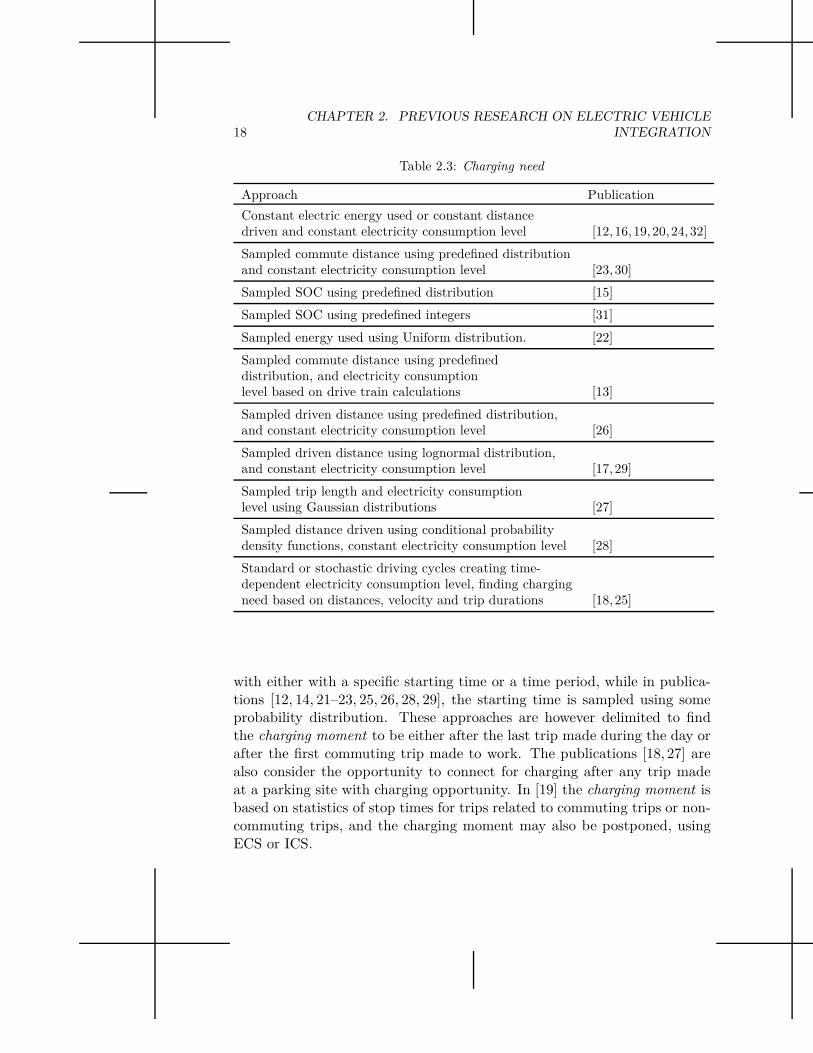
Different approaches of how to estimate the charging need is presented inTable 2.3. The charging need reflects the approach to find the electricity thatis used by the vehicle during driving and therefore may be transferred fromthe grid to the battery when connecting for charging. The electricity that isused by the vehicle may be estimated either on a daily basis, for each drivingoccasion, or as the electricity transferred at a charging event. It can be seenthat the publications [12, 16, 19, 20, 24, 32] make assumptions of constantelectricity used to determine the charging need. The publications [13, 15,17, 22, 23, 26–31] are instead assuming either some predefined probabilitydistributions or integers in order to sample either the electricity used orthe traveled distance before charging, but only [28] treats these variablesas dependent on each other. The assumptions made in publications [18,25]are further developed when they find the charging need in time based onelectricity consumption levels, distances driven, velocities and trip durations.The time-dependent movement may thus be captured with models based onthese assumptions. This enables knowledge of the time-dependent state ofcharge (SOC), charging need or available energy capacity when a vehiclearrives at any parking location with charging opportunity.
Charging moment
The charging moment represents when the vehicle battery is charged. Itcould be modeled either as the connecting time, i.e. the time that thecharging starts, or as the time period that the vehicle is connected. Forpublications [13, 15–17, 20, 24, 30–32], the charging moment is predefined
18CHAPTER 2. PREVIOUS RESEARCH ON ELECTRIC VEHICLE
INTEGRATION
Table 2.3: Charging need
Approach Publication
Constant electric energy used or constant distancedriven and constant electricity consumption level [12, 16,19, 20, 24, 32]
Sampled commute distance using predefined distributionand constant electricity consumption level [23, 30]
Sampled SOC using predefined distribution [15]
Sampled SOC using predefined integers [31]
Sampled energy used using Uniform distribution. [22]
Sampled commute distance using predefineddistribution, and electricity consumptionlevel based on drive train calculations [13]
Sampled driven distance using predefined distribution,and constant electricity consumption level [26]
Sampled driven distance using lognormal distribution,and constant electricity consumption level [17, 29]
Sampled trip length and electricity consumptionlevel using Gaussian distributions [27]
Sampled distance driven using conditional probabilitydensity functions, constant electricity consumption level [28]
Standard or stochastic driving cycles creating time-dependent electricity consumption level, finding chargingneed based on distances, velocity and trip durations [18, 25]
with either with a specific starting time or a time period, while in publica-tions [12, 14, 21–23, 25, 26, 28, 29], the starting time is sampled using someprobability distribution. These approaches are however delimited to findthe charging moment to be either after the last trip made during the day orafter the first commuting trip made to work. The publications [18, 27] arealso consider the opportunity to connect for charging after any trip madeat a parking site with charging opportunity. In [19] the charging moment isbased on statistics of stop times for trips related to commuting trips or non-commuting trips, and the charging moment may also be postponed, usingECS or ICS.
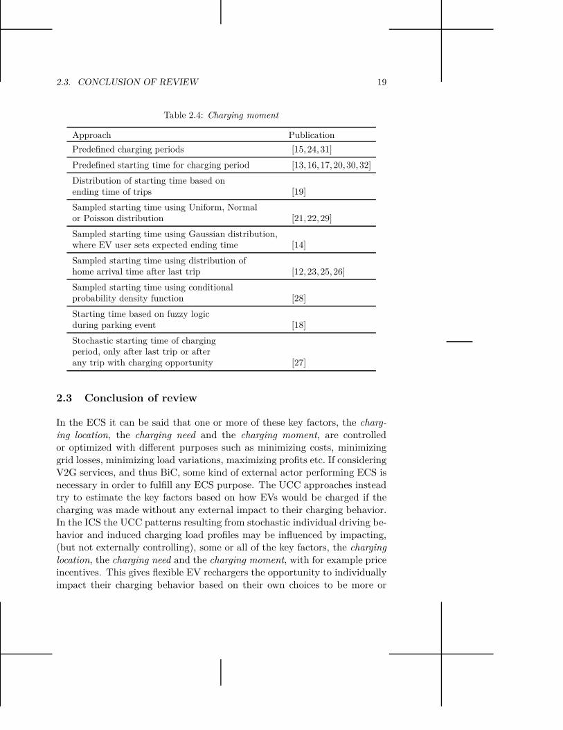
2.3. CONCLUSION OF REVIEW 19
Table 2.4: Charging moment
Approach Publication
Predefined charging periods [15, 24, 31]
Predefined starting time for charging period [13, 16, 17, 20,30, 32]
Distribution of starting time based onending time of trips [19]
Sampled starting time using Uniform, Normalor Poisson distribution [21, 22, 29]
Sampled starting time using Gaussian distribution,where EV user sets expected ending time [14]
Sampled starting time using distribution ofhome arrival time after last trip [12, 23, 25, 26]
Sampled starting time using conditionalprobability density function [28]
Starting time based on fuzzy logicduring parking event [18]
Stochastic starting time of chargingperiod, only after last trip or afterany trip with charging opportunity [27]
2.3 Conclusion of review
In the ECS it can be said that one or more of these key factors, the charg-ing location, the charging need and the charging moment, are controlledor optimized with different purposes such as minimizing costs, minimizinggrid losses, minimizing load variations, maximizing profits etc. If consideringV2G services, and thus BiC, some kind of external actor performing ECS isnecessary in order to fulfill any ECS purpose. The UCC approaches insteadtry to estimate the key factors based on how EVs would be charged if thecharging was made without any external impact to their charging behavior.In the ICS the UCC patterns resulting from stochastic individual driving be-havior and induced charging load profiles may be influenced by impacting,(but not externally controlling), some or all of the key factors, the charginglocation, the charging need and the charging moment, with for example priceincentives. This gives flexible EV rechargers the opportunity to individuallyimpact their charging behavior based on their own choices to be more or

20CHAPTER 2. PREVIOUS RESEARCH ON ELECTRIC VEHICLE
INTEGRATION
less willing to participate in for example load shifting activities encouragedwith price incentives or such. Both the ECS and the UCC approach areof importance when it comes to study and quantify the impact that EVCmay have to the power system and the load profile. However, it could beargued that people in general would rather not like to be controlled, or lettheir vehicle charging be controlled by external units, when no other resi-dential electricity-dependent activity is externally controlled yet, but thatthey would rather have the choice to charge their vehicle as they please, ifthere are choices available. This is the reason why considering ICS becomesimportant.
Gap of knowledge
There is currently a need for EVC models in order to estimate load profilesrelated to an EV introduction in the power system. The EVC models may bebased on different approaches of the key factors, dependent on the purpose ofthe model, which could be to model ECS, UCC or ICS. This thesis presentsfour different EVC models based on different combinations of assumptionsregarding the key factors in order to meet different purposes of estimatingEVC load profiles. These models are referred to as EVC-A, EVC-B, EVC-C and EVC-D. Each model intends to fill the respectively research gapsidentified in the following sections. The four models EVC-A to EVC-D areintroduced in Chapter 3.
Research gap 1: Motivation for model EVC-A
With EVC the peak load could increase especially with UCC. In areas wherethe grid is dimensioned close to the load limit, which often is set by trans-former capacity limitations; an additional load from EVs could force in-vestments in the grid infrastructure. The transformer is considered as animportant component in the grid due to potential severe and economic con-sequences upon failure, why it is important to evaluate EVC impact on thiscomponent. In [33] the cost of transformer wear, and other impact, werecalculated based on travel survey data to find the potential for communica-tion methods in controlling battery charging. However, there has been littlework done in transformer hotspot temperature rise and transformer loss oflife, due to an electric vehicle introduction and related EVC impact, whyit becomes important to estimate overloading on components due to EVCpatterns.

2.3. CONCLUSION OF REVIEW 21
Research gap 2: Motivation for model EVC-B
The level of EVC at home may result in large load variations and loadpeaks. Therefore, it becomes important to quantify the impact on the elec-tric power system due to PHEV home-charging patterns. No previous studyhas captured the variations in the households’ differentiated load profiledue to PHEV home-charging together with and related to other electricity-dependent residential activities. Therefore it is important to capture theresidential electricity-dependent activities performed including and in rela-tion to the electric vehicle usage if wanting to simulate and estimate theelectricity consumption in households.
Research gap 3: Motivation for model EVC-C
The level of EVC at any parking location with charging opportunity mayimpact the overall load with greater load variations and load peaks. TheEVC-B model only accounts for UCC and the charging location to be athome, neglecting to consider also other charging opportunities. In [34] EVCbehavior was instead described with a Markov Chain model, allowing thecharging location to be at several parking locations with charging oppor-tunities. That publication does consider the charging moment to occur atseveral times during the day related to the driving behavior, parking eventsand additional charging opportunities. However, in that model the time formovement was constant; one time step, and the EV could not remain in themovement state after entering it, but needed to change state into a parkingstate in next time step where a distance driven during the movement periodwas sampled. That approach thus did not capture the dependence betweenthe time for movement and the consumption during that movement, buttreats them separately, losing the time-dependency of the consumption dur-ing the movement, which affects the charging need. Moreover, the potentialof using EV batteries as flexible loads will probably depend on the randomparking events, with related charging opportunities and costs, and there willexist a potential only if some level of flexibility is assumed for the driving andcharging behavior. Making the vehicle batteries available for charging alsoin order to meet load variations thus assumes some level of flexibility for theEV user, when it comes to charging preferences. This highlights the impor-tance of developing models that take into account the time-dependency ofthe EV movement and the consumption during that movement to evaluatethe impact of EVC and eventual charging flexibility.

22CHAPTER 2. PREVIOUS RESEARCH ON ELECTRIC VEHICLE
INTEGRATION
Research gap 4: Motivation for model EVC-D
The trips made with an EV may have different purposes and these maybe related to charging opportunities that would impact the time-dependentEVC load profile. Additional factors that may impact the EVC load esti-mations are the prospective usage of a second fuel and fast charging option.Previous research with the general purpose to find the load impact of antic-ipated future EVC behavior on the grid does not consider the dependencyof all individual and stochastic parking events related to the type-of-tripincluding the eventual need to drive on a second fuel or use fast charging. Ittherefore is important to include these considerations in the EVC modeling.
Chapter 3
Modeling electric vehicle charging
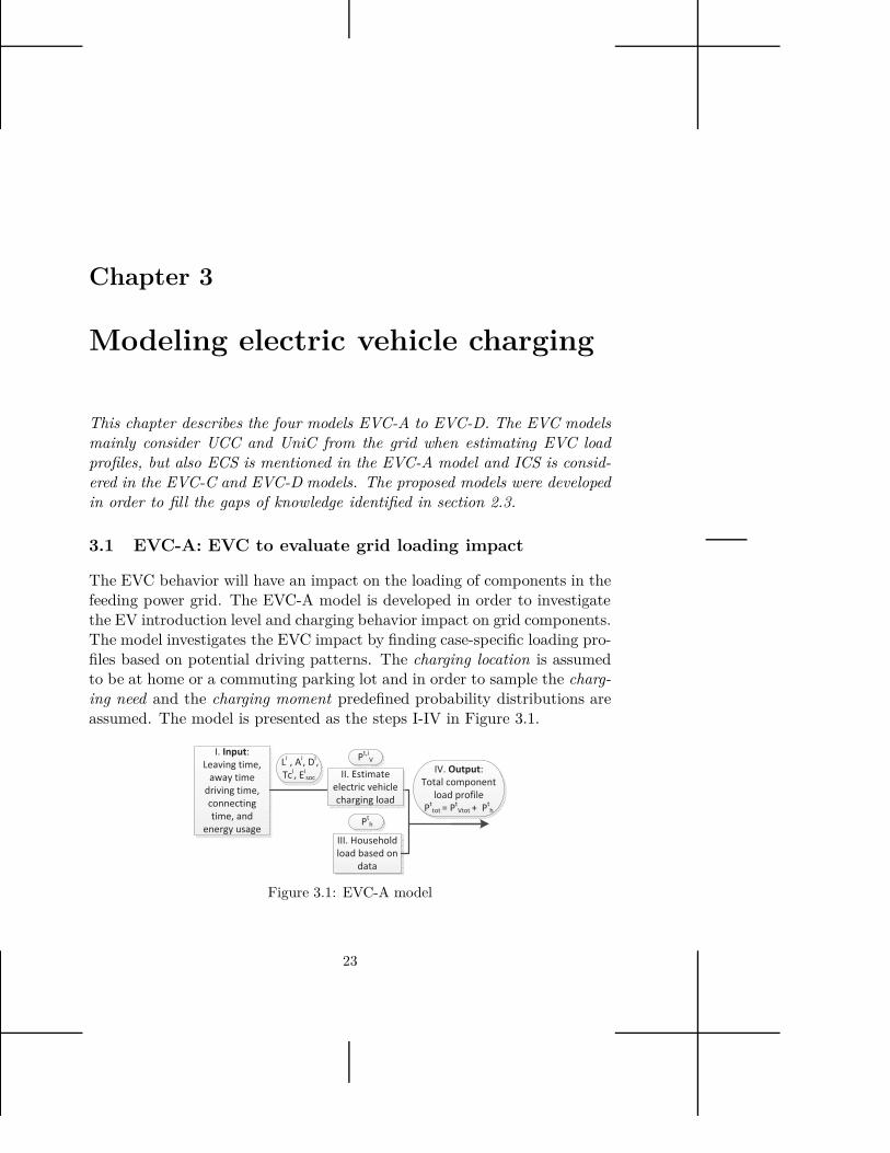
This chapter describes the four models EVC-A to EVC-D. The EVC modelsmainly consider UCC and UniC from the grid when estimating EVC loadprofiles, but also ECS is mentioned in the EVC-A model and ICS is consid-ered in the EVC-C and EVC-D models. The proposed models were developedin order to fill the gaps of knowledge identified in section 2.3.
3.1 EVC-A: EVC to evaluate grid loading impact
The EVC behavior will have an impact on the loading of components in thefeeding power grid. The EVC-A model is developed in order to investigatethe EV introduction level and charging behavior impact on grid components.The model investigates the EVC impact by finding case-specific loading pro-files based on potential driving patterns. The charging location is assumedto be at home or a commuting parking lot and in order to sample the charg-ing need and the charging moment predefined probability distributions areassumed. The model is presented as the steps I-IV in Figure 3.1.
I. Input:
Leaving time,
away time
driving time,
connecting
time, and
energy usageIII. Household
load based on
data
IV. Output:
Total component
load profile
Pttot = P
tVtot + P
th
Pt,i
V
Pth
II. Estimate
electric vehicle
charging load
Li, A
i, D
i,
Tci, E
isoc
Figure 3.1: EVC-A model
23

24 CHAPTER 3. MODELING ELECTRIC VEHICLE CHARGING
Estimation of electric vehicle usage
The EVC is here modeled as a load profile in discrete time based on stochas-tic variables. The charging pattern is based on that the electricity consump-tion takes place when the EV is used, creating a charging need, and the loadprofile emerge during the charging moment. Index t represents each timestep for t = 1, ..., T where T is the total number of time steps and the i rep-resents each vehicle. In the model the EVC need from the grid is assumedto correspond to the electricity use of the EV.
In step I in Figure 3.1 the model input are introduced. The variablesare case-specific, for details see section 4.1. The charging moment occurswhen the EV is parked and connected at time T ci, until the battery is fullycharged. In Cases 1-3 the connecting time T ci depends on the leaving timefrom home Li, and either the time period the EV user is away from homeAi or the driving time Di. In these cases the starting time of a trip isthe leaving time Li, and the connecting time T ci is the time when arrivinghome or to a parking site at work. In Case 1 the variables leaving time fromhome Li, away time Ai and electricity use Ei
soc, are sampled independentlyof each other. This allows an EV user to leave home with the vehicle, beaway from home a time period during the day, and use the EV any timeduring that time period. The variables in Case 1 should be chosen to ensurethat maximum electricity use Emax,i
soc does not exceed what potentially couldbe used during the minimum away time Amin,i. The EVC is in this caseassumed to occur at home and the connecting time T ci
1 is calculated as:
T ci1 = Li + Ai. (3.1)
In Case 2 the electricity used Eisoc, depends on the sampled driving time Di,
and parameters for the velocity vm, and the consumption cm when driving:
Eisoc = Dimvmcm (3.2)
The EVC in this case is assumed to occur at a commuting parking place orparking site at work and the connecting time T ci
2 is calculated as:
T ci2 = Li + Di (3.3)
Case 3 is a case including an area with both Case 1 and Case 2 EVs. InCases 4 and 5 the daily EV electricity use Ei
soc is sampled. In Case 4 theEVC is assumed to occur at home, but the EVC is postponed to start atlater hours than in Case 1. This is done by sampling the connecting time

3.1. EVC-A: EVC TO EVALUATE GRID LOADING IMPACT 25
T ci4 close to a mean time. In Case 5 an ECS is assumed to be able to control
an amount of used EVs connected at any charging location by distributingthe EVC during hours of the day with less overall demand. This is doneby sampling the connecting times T ci
5 more widely distributed over valleyhours during the day.
Estimation of load profiles
In step II in Figure 3.1 the EVC load is estimated. The EVC load at timestep t for a vehicle i is P t,i
V is based on the charging power of Pc whencharging. Each EV is assumed to stay connected for a charging time periodCti until the battery is fully charged. The length of the EVC time periodCti for EV i is estimated as:
Cti = Eisoc/Pc. (3.4)
With charging power Pc, the load P t,iV for each vehicle i at time t is simulated
according to:
P t,iV =
{
Pc if charging
0 else.(3.5)
The expected value E[P tV ] of the electric vehicle load P t
V at time t withMonte Carlo simulations for n samples is:
E[P tV ] =
1
n
n∑
i=1
P t,iV . (3.6)
The total electric vehicle load P tV tot at time t for Ntot vehicles is estimated
as:P t
V tot = NtotE[P tV ]. (3.7)
In step III in Figure 3.1 the mean household load is estimated. The house-hold load P t
h at time t is estimated as the normalized load curve P tn,h mul-
tiplied with a total number of households H, and with the assumed averageconsumption Bh kWh per day and apartment.
P th = HP t
n,hBh. (3.8)
In step IV in Figure 3.1 the total load profile is obtained. The total meanload profile P t
tot at time t is estimated as:
P ttot = P t
V tot + P th. (3.9)

26 CHAPTER 3. MODELING ELECTRIC VEHICLE CHARGING
In Case 3 the estimate of the mean load profile is obtained by adding theP t
V tot from EVC based on Case 1 to the P tV tot from EVC based on Case 2.
The overall simulation algorithm is presented in Figure 3.2, specifying eachstep in the simulation.
Start, i=0, t=0
i = i +1
Sample Tci
t = t +1
Calculate EVC
load profile
Pt,i
V
E[PtV]
Esimate total load
profile
Estimate mean
EVC load
Pttot
Estimate hotspot
temperature and loss of
life, using thermal model
equations in Paper II
i < n
t < T
Figure 3.2: EVC-A simulation algorithm
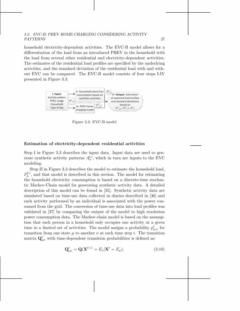
3.2 EVC-B: PHEV home-charging considering activity
patterns
The EVC-B model combines PHEV usage, based on residential activities,with the household electricity usage due to other electricity-dependent ac-tivities performed at home. The charging location is considered to be athome, while the charging need and the charging moment are based on syn-thetic residential and electricity-dependent activities in the household. TheEVC-B model considers the possibility to connect for charging after sev-eral stochastic individually made trips that impact the charging need basedon assumptions of usage probability. The model for synthetic activity gen-eration of residents’ performed activities was developed in [35]. Statisticsfrom available time of use data are used as model input to simulate the
3.2. EVC-B: PHEV HOME-CHARGING CONSIDERING ACTIVITY
PATTERNS 27
household electricity-dependent activities. The EVC-B model allows for adifferentiation of the load from an introduced PHEV in the household withthe load from several other residential and electricity-dependent activities.The estimates of the residential load profiles are specified by the underlyingactivities, and the standard deviation of the residential load with and with-out EVC can be compared. The EVC-B model consists of four steps I-IVpresented in Figure 3.3.
III. PHEV home
charging model
II. Household electricity
consumption based on
synthetic activities
IV. Output: Estimation
of expected load profiles
and standard deviations
based on
Pt,i
tot = Pt,i
V + Pt,i
h
Pt,i
V
Pt,i
hI. Input:
Activity pattern
PHEV usage
Household
Type of day
At,i
m
Figure 3.3: EVC-B model
Estimation of electricity-dependent residential activities
Step I in Figure 3.3 describes the input data. Input data are used to gen-erate synthetic activity patterns At,i
a , which in turn are inputs to the EVCmodeling.
Step II in Figure 3.3 describes the model to estimate the household load,P t,i
h , and that model is described in this section. The model for estimatingthe household electricity consumption is based on a discrete-time stochas-tic Markov-Chain model for generating synthetic activity data. A detaileddescription of this model can be found in [35]. Synthetic activity data aresimulated based on time-use data collected in diaries described in [36] andeach activity performed by an individual is associated with the power con-sumed from the grid. The conversion of time-use data into load profiles wasvalidated in [37] by comparing the output of the model to high resolutionpower consumption data. The Markov-chain model is based on the assump-tion that each person in a household only occupies one activity at a giventime in a limited set of activities. The model assigns a probability pt
µ,ν fortransition from one state µ to another ν at each time step t. The transitionmatrix Qt
µν with time-dependent transition probabilities is defined as:
Qtµν = Q(Xt+1 = Eν |Xt = Eµ). (3.10)

28 CHAPTER 3. MODELING ELECTRIC VEHICLE CHARGING
Here µ, ν ∈ {1, ..., N} represent states for the electricity-dependent activ-ities that can be performed by residents in a household and N is the numberof activities. Equation (3.10) satisfies the Markov property since a state isdependent only on the previous state. The probability for an individual tooccupy any state at a given time t is
∑Nµ=1 pµ,t = 1. The probability that
the process occupies a particular state at time t is as defined in [38]:
ptµ = p(Xt = Eµ). (3.11)
The output of the Markov-chain is the time-dependent activities for timet ∈ [1, ..., T ], sample i and activity a ∈ [1, ..., N ]. If an entry of At,i
a is equalto one then activity a is performed at t for sample i, and if At,i
a is zerothen activity a is inactive at time t. Each individual has its own sampledbehavior, but some electricity-dependent activities may be conducted at thesame time for more than one individual, and these are described in detailin [35]. The household load is defined as P t,i
h and is based on the electricityconsumption P
At,ia
from the electricity-dependent activities:
P t,ih =
N∑
a=1
PA
t,ia
. (3.12)
Estimation of electric vehicle usage
This section describes step III in Figure 3.3, where the EVC is modeled. Thesynthetic residential activities are used to estimate the EVC load profiles aswell as the household electricity consumption. The PHEV is here assumedto be used with a probability of pcar, when the activity state changes into’Away’, At,i
1 = 1 for an individual in the household. The SOCt,i decreasesbased on the electricity consumption when the vehicle is used, thus whenK < pcar is satisfied. K is a stochastic variable with a uniform distributionK ∈ U(0, 1), that is sampled each time a potential driver leaves the house-hold. The vehicle and driver are assumed to be away during the number oftime steps following upon a change into ’Away’, until returning home andAt,i
1 , 1. The consumption Ct(vtm, ct
m, Cts) while driving depends on the
velocity vtm, the consumption ct
m when driving and the season, modeled byseasonal coefficients Ct
s. The velocity vm and consumption cm are treated asconstants in this model, using average values. During charging at a powerof Pc, the SOCt,i increases according to equation (3.13), until the batteryis fully charged, SOCt,i = SOCi
max, or the resident uses the car again. The

3.2. EVC-B: PHEV HOME-CHARGING CONSIDERING ACTIVITY
PATTERNS 29
SOC changes in each time step according to: (vtm)
SOCt+1,i =
SOCt,i − Ct∆t if consuming,
SOCt,i + Pc∆t if charging,
SOCt,i else.
(3.13)
If the SOC is running low and the vehicle still is performing a trip, thenthe PHEV is assumed to be running on a second fuel. To avoid a decreaseof battery lifetime, the SOC is limited to a minimum depth of discharge(DOD) which is decided by the fraction pdod. The SOCt,i in the battery isconstrained by:
pdodSOCimax ≤ SOCt,i ≤ SOCi
max. (3.14)
The EVC occurs when the resident returns home after a trip with the PHEV.The starting time of a trip and also the returning time after a trip with thevehicle are decided by the synthetic activities. The EVC is assumed to startinstantly when arriving home after a trip, inducing charging moment. TheEVC thus takes place when the car is parked at home, connected and notyet fully charged. The EVC load P t,i
V for sample i at time t is based on thecharging power Pc and the connected time period:
P t,iV =
{
Pc if charging,
0 else.(3.15)
In general, if data were to be found of times when a PHEV would injectpower to the grid, the battery may also be used as temporary electric powerproduction, with a negative P t,i
V allowing for V2G.
Estimation of load profiles
This section describes step IV in Figure 3.3 where the total load profile isestimated. The load profile P t,i
tot per household with EVC load is obtainedby adding the household consumption from the other electricity-dependentactivities P t,i
h :
P t,itot = P t,i
V + P t,ih (3.16)
For the stochastic variable W t,i = {P t,itot, P t,i
V , P t,ih , P
At,im
}, the mean value W t
and the standard deviation stw are estimated at time t based on n samples.
The mean load profile due to any electricity-dependent is estimated as:
W t =1
n
n∑
i=1
W t,i, (3.17)

30 CHAPTER 3. MODELING ELECTRIC VEHICLE CHARGING
and the standard deviation stw is estimated as:
stw =
√
√
√
√
1
n
n∑
i=1
(W t,i − W t,i)2. (3.18)
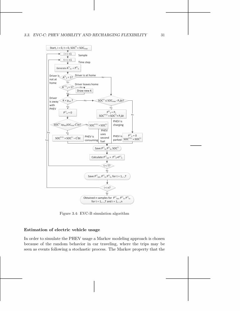
Simulation algorithm
The simulation algorithm for the EVC-B model is presented in Figure 3.4.The algorithm is shown for a case when each household is assumed to haveone PHEV and one driver. It would be possible to allow for more thanone driver per vehicle, and more than one vehicle per driver. The first casewould be illustrated by checking where all the individuals are located, athome or not, and sample if they are together, represented by one flowchartfor each driver, to find if they are out driving together or if one of themhas the vehicle. The second case would be illustrated by having more SOCparameters, denoted to specified vehicles, and then checking which vehicleis taken by which driver. However, these cases are not implemented in thecase study for simplifying reasons that shortens the simulation time, whythe algorithm is illustrated for one driver.
3.3 EVC-C: PHEV mobility and recharging flexibility
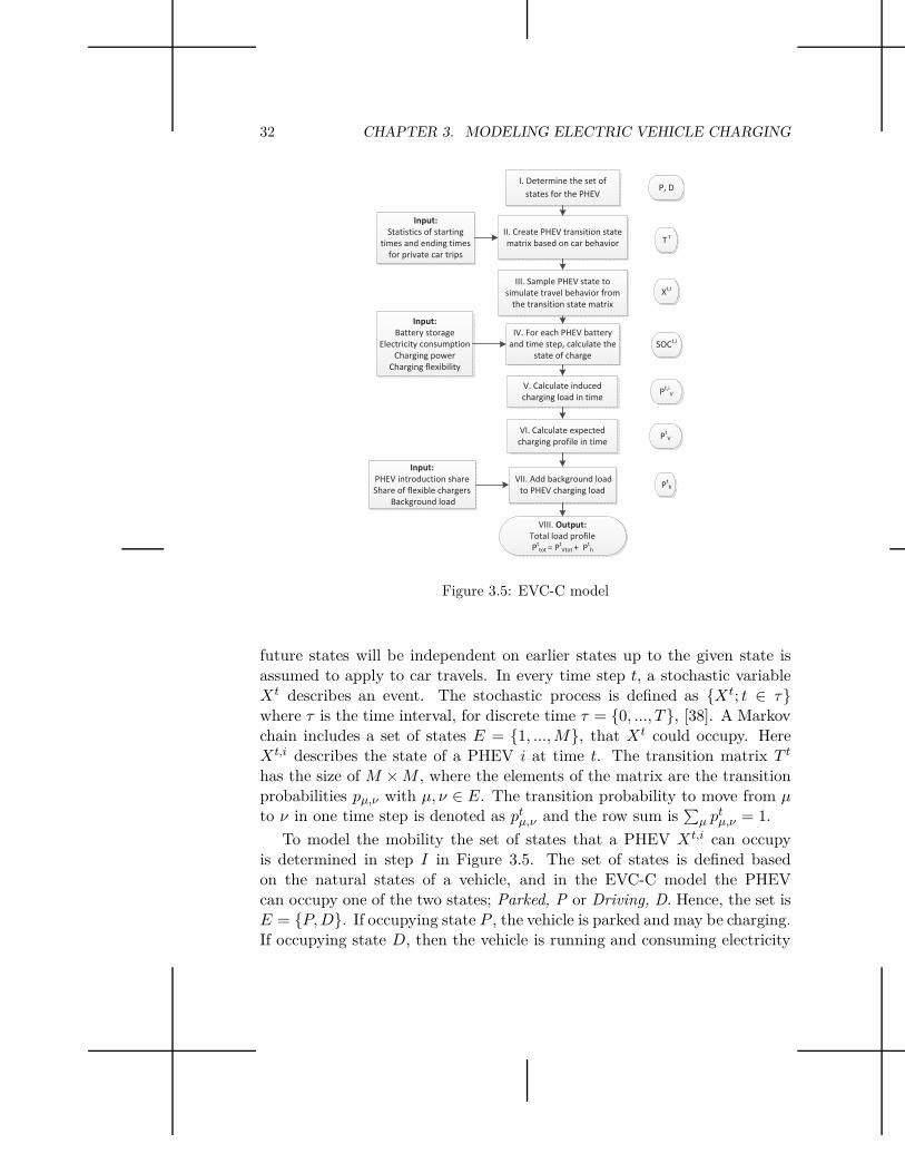
The EVC-C model allows for simulations of UCC and also ICS using charg-ing price sensitivity. The model captures the time-dependency of the con-sumption during the vehicle movement based on driving patterns to estimateexpected corresponding charging profiles. Starting times and ending timesfor private car trips are considered in order to model the mobility. Thecharging need is based on the velocity and electricity consumption when thevehicle is performing a trip. When capturing the time-dependent consump-tion during the vehicle movement, the charging need, the charging momentand the charging location can be estimated as a function of time, and thethree key factors are treated as dependent on each other. The EVC mayoccur at any parking event after a trip if there is a charging need. It is as-sumed that the EVC power may be measured and identified for each PHEV,for example with devices in the vehicle. The EVC-C model consists of thesteps I-VIII presented in Figure 3.5.
3.3. EVC-C: PHEV MOBILITY AND RECHARGING FLEXIBILITY 31
Start, i = 0, t = 0, SOC0
= SOCmax
i = i +1
Save Pt,i
tot, Pt,i
V, Pt,i
h, for t = 1,..,T
Yes
At-1,i
1 = 1?
K < pcar ? SOCt,i
SOCmax - Pc t?
SOCt,i
pdodSOCmax-Ct
t?
Yes
Pt,i
V = 0
SOCt+1,i
= SOCt,i
Pt,i
V = Pc
SOCt+1,i
= SOCt,i
+ Pc tP
t,iV = 0
PHEV is
consuming
PHEV is
charging
PHEV is
parked
YesYes
No
No
No
SOCt+1,i
= SOCt,iNo
Yes
Obtained n samples for Pt,i
tot, Pt,i
V, Pt,i
h,
for t = 1,...,T and i = 1,…,n
SOCt+1,i
= SOCt,i
– Ct
t
t = i +1
Driver is at home
t < T?
i < n?
No
Save Pt,i
V, Pt,i
h, SOCt,i
Yes
No
Sample
Time step
Generate At,i
m -> Pt,i
h
Calculate Pt,i
tot = Pt,i
V+Pt,i
h
PHEV
uses
second
fuel
At,i
1 = 1?
Yes
Driver leaves home
Driver is
not at
home
No
Driver
is away
with
PHEV
Draw new K
Figure 3.4: EVC-B simulation algorithm
Estimation of electric vehicle usage
In order to simulate the PHEV usage a Markov modeling approach is chosenbecause of the random behavior in car traveling, where the trips may beseen as events following a stochastic process. The Markov property that the
32 CHAPTER 3. MODELING ELECTRIC VEHICLE CHARGING
Input:
PHEV introduction share
Share of flexible chargers
Background load
VIII. Output:
Total load profile
Pttot = P
tVtot + P
th
Pth
Input:
Battery storage
Electricity consumption
Charging power
Charging flexibility
Tt
Input:
Statistics of starting
times and ending times
for private car trips
II. Create PHEV transition state
matrix based on car behavior
I. Determine the set of
states for the PHEV
III. Sample PHEV state to
simulate travel behavior from
the transition state matrix
P, D
Xt,i
IV. For each PHEV battery
and time step, calculate the
state of charge
SOCt,i
V. Calculate induced
charging load in time P
t,iV
VII. Add background load
to PHEV charging load
VI. Calculate expected
charging profile in time P
tV
Figure 3.5: EVC-C model
future states will be independent on earlier states up to the given state isassumed to apply to car travels. In every time step t, a stochastic variableXt describes an event. The stochastic process is defined as {Xt; t ∈ τ}where τ is the time interval, for discrete time τ = {0, ..., T }, [38]. A Markovchain includes a set of states E = {1, ..., M}, that Xt could occupy. HereXt,i describes the state of a PHEV i at time t. The transition matrix T t
has the size of M × M , where the elements of the matrix are the transitionprobabilities pµ,ν with µ, ν ∈ E. The transition probability to move from µto ν in one time step is denoted as pt
µ,ν and the row sum is∑
µ ptµ,ν = 1.
To model the mobility the set of states that a PHEV Xt,i can occupyis determined in step I in Figure 3.5. The set of states is defined basedon the natural states of a vehicle, and in the EVC-C model the PHEVcan occupy one of the two states; Parked, P or Driving, D. Hence, the set isE = {P, D}. If occupying state P , the vehicle is parked and may be charging.If occupying state D, then the vehicle is running and consuming electricity

3.3. EVC-C: PHEV MOBILITY AND RECHARGING FLEXIBILITY 33
from the battery given there is enough left. The states are illustrated inFigure 3.6. In order to sample the states for a PHEV i the transition matrix
Driving, DParked, P
ptPD
ptDP
ptPP p
tDD
Figure 3.6: Transition states
T t, is needed in step II in Figure 3.5. The transition state probabilitiesfor changing state are time-dependent, and a PHEV i can only occupy onestate at a certain time step t. The transition matrix T t, is defined as:
T t =
[
ptP P pt
P D
ptDP pt
DD
]
, t ∈ τ. (3.19)
The initial state probabilities S0,i for a vehicle i are:
S0,i =[
p0,iP , p0,i
D
]
. (3.20)
From these, the initial state X0,i for PHEV i may be sampled. In step IIIin Figure 3.5 time-dependent state sequences for each PHEV i is sampled.The probability for vehicle i to occupy a state P or D in the time step t + 1is St+1,i. St+1,i is equal to the row in the matrix T t which corresponds tothe state in time step t. If X0,i = P then one takes the first row in T 0,and samples the next state from the probabilities in this row. This is doneby comparing the probabilities in this row with a random number sampledfrom a uniform distribution K ∈ U(0, 1). A time-dependent state sequencefor a PHEV i is hereby created.
Estimation of transition probabilities
In order to find the elements of the matrix T t, probabilities may be estimatedfrom available car travel behavior data. In this section the estimates of thesetransition probabilities are described.
First, an initial number of parked vehicles is expressed as a share pP ofa total number ntot of vehicles:
n0P = ntotpP , (3.21)

34 CHAPTER 3. MODELING ELECTRIC VEHICLE CHARGING
The number nt+1P of parked vehicles in the next time step is then calculated
as:nt+1
P = ntP − nt+1
st + nt+1en , t ≥ 0, (3.22)
where ntst is the number of vehicle trips that are starting at time t + 1, and
nten is the number of vehicle trips that are ending at time t+1. The number
ntD of trips performed at time t is calculated as:
ntD = ntot − nt
P . (3.23)
The elements of the transition matrix T t are further estimated. The prob-ability pt
P D to change from state P into state D is estimated as:
ptP D =
ntst
ntP
. (3.24)
The probability ptDP to change state from D into P is estimated as:
ptDP =
nten
ntD
. (3.25)
The probability ptP P to remain in state P is estimated as:
ptP P = 1 − pt
P D, (3.26)
and the probability ptDD to remain in state D is estimated as:
ptDD = 1 − pt
DP . (3.27)
State of charge
In order to estimate the UCC load profile, the time-dependent SOC needsto be calculated in step IV in Figure 3.5. Based on an assumption that thesimulation starts in the morning after charging during a night, the batteryis initially assumed to be fully charged for each vehicle i:
SOC0,i = SOCimax. (3.28)
It is assumed that SOCt,i = 0 corresponds to a lowest allowed energy levelin the battery. The SOC of the battery thus lies in between 0 and a fullycharged battery with storage SOCi
max:
0 ≤ SOCt,i ≤ SOCimax. (3.29)

3.3. EVC-C: PHEV MOBILITY AND RECHARGING FLEXIBILITY 35
The SOC for vehicle i at time step t + 1 is calculated to increase with thecharging power Pc, during EVC, and decrease with the electricity consump-tion Cm, when the vehicle is running on electricity:
SOCt+1,i =
SOCt,i + Pc∆t if charging,
SOCt,i − Cm∆t if consuming,
SOCt,i else.
(3.30)
The electricity consumption Cm when driving could be a time-dependentvariable, but is here assumed to be constant. The SOCt,i will remain thesame as in the previous time step in two cases: If the vehicle is parked andthe SOC is too close to the SOCi
max to be charged in the next time step,and if the vehicle is running but has too low SOC for using electricity fromthe battery in the next time step. If the vehicle has too low SOC but stilloccupies the driving state D, then the vehicle is assumed to run on a secondfuel.
Charging flexibility
To model charging flexibility, the following ICS is used: Time periods t ∈TF , are defined for when the electricity charging price is assumed to besufficiently high for a share pF , of the individual EV rechargers to becomeflexible. The flexible rechargers agree on postponing their battery chargingif the SOC level for vehicle i is not below a certain fraction F i
min. For flexiblerechargers the following condition is added to equation (3.30), in step IV inFigure 3.5.
SOCt+1,i = SOCt,i if t ∈ TF , SOCt,i > SOCimaxF i
min. (3.31)
To model a price-limit P iL for which a flexible recharger i decides to post-
pone the charging moment, the mean daily charging price Ep is used. Adaily price-limit P i
L, for the flexible EVC is set individually for each vehiclerecharger i as:
P iL = Ep + kiEp (3.32)
where ki is sampled daily, but is constant all day for an individual i, froma uniform distribution ki ∈ U(a, b). The time periods t ∈ TF , for when theflexible recharger i is postponing the EVC is defined by the constraint:
t ∈ TF : Etp < P i
L (3.33)
This means that a flexible recharger i has an individual price-limit P iL that
depend on a forecasted daily price profile Etp.

36 CHAPTER 3. MODELING ELECTRIC VEHICLE CHARGING
Estimation of load profiles
The EVC load P t,iV for vehicle i at time step t is calculated in step V in
Figure 3.5:
P t,iV =
{
Pc if charging,
0 else.(3.34)
The expected load profile E[P tV ] for one vehicle is estimated as the mean
value using Monte Carlo simulations for n samples in step V I in Figure 3.5:
E[P tV ] ≈ 1
n
n∑
i=1
P t,iV . (3.35)
The standard deviation stV is estimated as:
stV =
√
√
√
√
1
n − 1
n∑
i=1
(P t,iV − P t
V )2. (3.36)
The total EVC load P tV at time t for Ntot vehicles is estimated in V II in
Figure 3.5 as:P t
V tot = NtotE[P tV ]. (3.37)
The total load profile is estimated by adding a daily overall load P tB to
the expected mean load from a number Ntot of vehicles in steps V III inFigure 3.5:
P ttot = P t
V tot + P tB . (3.38)
3.4 EVC-D: PHEV utilization considering type-of-trip and
recharging flexibility
With the model EVC-D it is possible to simulate detailed PHEV mobility be-havior due to the type-of-trip and related UCC and refueling opportunities.The electricity consumption from the battery or the consumption of a sec-ond fuel takes place during the vehicle movement related to the type-of-tripconducted. The opportunity to connect for charging after any type-of-trip ina parking event with charging opportunity is considered, making it possibleto estimate EVC impact to the overall load.
The EVC-D model takes into account detailed starting times and endingtimes for private car trips dependent on the type-of-trip and relates them

3.4. EVC-D: PHEV UTILIZATION CONSIDERING TYPE-OF-TRIP AND
RECHARGING FLEXIBILITY 37
to time-dependent consumption levels and charging opportunities. The keyfactors are treated as stochastic and dependent on each other. The charg-ing moment is considered to be after any time-dependent type-of-trip at acharging location which is a parking site with related charging opportunity.The charging need is based on the consumption when the vehicle is in move-ment, which is dependent on the type-of-trip and the type-of-trip-dependentvelocity.
ICS is modeled using an individual charging price sensitivity which is de-ciding if the charging should be postponed or not and if refueling the tankwith second fuel or fast charging is made. The ICS due to charging pricesensitivity affect the EVC load profiles, due to the individual price-limitdependent on the charging-, fast-charging and gasoline price. It is assumedthat the EVC power may be measured and identified for each PHEV, forexample with identification and electricity measurement devices in the ve-hicle. The EVC-D model is presented in Figure 3.7 with the steps I − IX.
Estimation of electric vehicle usage
A Markov model was used due to the random behavior in traveling wherethe trips are seen as a following a stochastic process. The Markov property,that future states are independent on earlier states up to the given state,is assumed to apply to car travels. The probabilities in the Markov chainare parameterized to replicate observed driving patterns which are time-of-day and day-of-week dependent. The velocity, electricity consumption andsecond fuel consumption when driving are parameterized in the case studyin section 4.4 to be type-of-trip-dependent.
In each time step t, a stochastic variable Xt describes an event and thestochastic process is defined as {Xt; t ∈ τ} where τ is the time intervalfor discrete time τ = {0, ..., T }, [38]. The Markov chain includes a set ofstates that Xt could occupy, and to model the PHEV mobility, the set ofstates that a PHEV can occupy is based on the natural states of a vehicle inuse: driving and parked. Here, the PHEV states are set to: Parking state,{A,B,...,NP } or Driving state, {1,...,ND} in step I in Figure 3.7. Hence,the set is E = {A, ..., NP , 1, ..., ND}.
In step II in Figure 3.7 corresponding charging opportunities in parkingstates related to the type-of-trip are defined. The parking states A − NP
represent several parking sites where the PHEV may be parked and perhapscharged. The driving states represent several type-of-trips performed by the

38 CHAPTER 3. MODELING ELECTRIC VEHICLE CHARGING
IX. Output: Obtain load profiles, standard deviations, electricity
usage, second fuel usage, emissions and costs
I. Determine the set of states
for the PHEV
PHEV mobility data:
Statistics of starting times
and ending times for
different type-of-trips with
private car
Initial PHEV values:
Initial battery storage
Initial tank storage
Initial state
PHEV state parameters:
Charging power due to parking
Velocity due to type-of-trip
Electricity and second fuel use
due to type-of-trip
Flexibility parameters:
Individual charging price-limit
Minimum battery level accepted
Second fuel cost parameter
PHEV refueling cost:
Electricity charging price
Fixed- and fast charging cost
Second fuel cost parameter
Second fuel cost
Addidional data:
Overall load
Energy and CO2 content
in fuel
Input:
III. Create PHEV transition
state matrix based on car
travel behavior
II. Create driving states and
parking states and define
corresponding charging
opportunity due to the
type-of-trip
IV. Generate state sequences
to simulate travel behavior
from the transition state
matrix
V. For flexible and inflexible
PHEVs calculate state of
charge and state of tank in
time with refilling and driving
due to the type-of-trip
VI. Calculate utilization
parameters; distance driven,
electricity usage, second fuel
usage, utilization cost and
charging load for each PHEV
and time step
VII. Run Monte Carlo
simulations and estimate
expected time-dependent
utilization parameters
VIII. Add overall load to PHEV
charging load
Figure 3.7: EVC-D model
PHEV between the different parking locations. If the PHEV occupy any ofthe driving states 1 − ND, the PHEV is running and consuming electricityfrom the battery given there is enough left, otherwise the second engineand its fuel is used. After occupying a parking state, the PHEV can stayor end up in any driving state. In the driving states, the PHEV can havedifferent electricity or fuel consumption due to the type-of-trip. The parkingstates offer different charging opportunities. After occupying a driving statethe PHEV can end up in a parking state dependent on the type-of-tripconducted.
The transition probability to change state from µ to ν in one time stepis denoted as pt
µ,ν where∑ν
µ=1 ptµ,ν = 1. A PHEV, i can only occupy one
state Xt,i at a certain time step t. The transition matrix T t has the size of

3.4. EVC-D: PHEV UTILIZATION CONSIDERING TYPE-OF-TRIP AND
RECHARGING FLEXIBILITY 39
M × M = (NP + ND) × (NP + ND), where the elements of the matrix arethe time-dependent transition probabilities pt
µ,ν with µ, ν ∈ E as step IIIin Figure 3.7. Several elements in T t are zero since changing from a drivingstate to another driving state requires the PHEV to occupy a parking statefirst. The same holds for changing state from a parking state to anotherparking state when the PHEV needs to occupy a driving state first. TheMarkov chain starts in an initial state at time step 0, by letting the PHEVoccupy one of the states in the set E. The initial state probabilities S0,i are:
S0,i =[
p0,iA . . . p0,i
NDp0,i
1 . . . p0,iND
]
. (3.39)
From these, the initial state X0,i for PHEV i may be sampled. The prob-ability for vehicle i to occupy a state {A, ..., NP , 1, ..., ND} in the time stept + 1 is St+1,i. St+1,i is equal to the row in the matrix T t which correspondsto the state in time step t. If the PHEV is parked in state A at time t,thus Xt,i = A, then one takes the first row in T t and samples the next stateXt+1,i, from the probabilities in this row. This is done by comparing theprobabilities in this row with a random number sampled from a uniform dis-tribution K ∈ U(0, 1). Time-dependent state sequences for events of eachPHEV i may hence be generated in step IV in Figure 3.7.
Estimation of transition probabilities
In order to find the elements of the matrix T t, transition probabilities maybe estimated from available car travel behavior data, and these estimates aredescribed here. First an initial number of parked vehicles n0
P is expressed asthe sum of the shares pP x of the maximum numbers n0
x,tot of parked PHEVsin x = {A, ..., NP }:
n0P =
NP∑
x=A
n0x,totpP x, (3.40)
The initial number of driving vehicles n0D is expressed as the sum of the
initial amount n0Dz of driving PHEVs with type-of-trip z = {1, ..., ND}:
n0D =
ND∑
z=1
n0Dz. (3.41)
The total number of parked PHEVs in the next time step is:
nt+1P = nt
P −ND∑
z=1
nt+1st,z +
ND∑
z=1
nt+1en,z, t ≥ 0, (3.42)

40 CHAPTER 3. MODELING ELECTRIC VEHICLE CHARGING
where ntst,z is the amount of type-of-trips z = {1, ..., ND} starting, and nt
en,z
is the amount of type-of-trips z = {1, ..., ND} ending at time t. The totalnumber nt
Dz of driving PHEVs in driving state z is calculated as:
nt+1Dz = nt
Dz + nt+1st,z − nt+1
en,z, t ≥ 0, (3.43)
It is assumed that the probability to start a type-of-trip z is independenton current parking state. The elements of the time-dependent transitionmatrices T t is now estimated as:
ptxz =
ntst,z
ntP
, (3.44)
for changing from any parking state into driving state z, and
ptzx =
nten,z
ntDz
, (3.45)
for changing from driving state z into parking state x. For remaining inparking state xx the element is calculated as:
ptxx = 1 −
ND∑
z=1
ptxz. (3.46)
For remaining in driving state zz the element is calculated as:
ptzz = 1 −
NP∑
x=A
ptzx, (3.47)
Electricity driving mode
In order to estimate the UCC load profile and second fuel usage, the time-dependent SOC and state of tank (SOT) are calculated in step V . TheSOC for a PHEV i at time step t + 1 increases if the PHEV is charging withPc∆t/ηc where the charging power is Pc, the charging efficiency is ηc, and thetime step length is ∆t. The charging power Pc may vary depending on forexample the time, the charging location or the charging moment. Here, thecharging power is assumed to be depending on the parking state. The charg-ing power is assumed to be either slow charging with Pc1, medium chargingwith Pc2 or fast charging with Pc3. If the PHEV is consuming electricity theSOC decreases with Cm∆t/ηdc where ηdc is the discharging efficiency fromthe battery. The consumption level Ct
m(vtm, ct
m) is a function of the velocity

3.4. EVC-D: PHEV UTILIZATION CONSIDERING TYPE-OF-TRIP AND
RECHARGING FLEXIBILITY 41
vtm, and the kilometer fuel use ct
m which here are time-dependent variablesthat are sampled from probability distributions related to the type-of-trip.If the PHEV is parked without charging or running on the second fuel, theSOC remains the same as in previous time step. Hence, the following holds:
SOCt+1,i =
SOCt,i + Pc∆t/ηc when charging,
SOCt,i − Ctm∆t/ηdc when consuming,
SOCt,i else.
(3.48)
For each PHEV i, the battery has an initial level of SOC0,i and followinglimitations:
0 ≤ SOCt,i ≤ SOCimax. (3.49)
The PHEV utilization is estimated for each PHEV i and time t in step V I inFigure 3.7. The cumulative distance driven with electricity Et,i
d for vehiclei is:
Et+1,id =
Et,id + vt
m∆t if running on electricity,
Et,id else.
(3.50)
The cumulative electricity consumed from the grid Et,iE for vehicle i is:
Et+1,iE =
Et,iE + Pc∆t/ηc if charging,
Et,iE else.
(3.51)
The cumulative variable electricity charging cost Et,iC for vehicle i in time
step t + 1 is:
Et+1,iC =
Et,iC + Et
pPc∆t/ηc if charging,
Et,iC else.
(3.52)
Second fuel driving mode
The second fuel usage can be calculated for when the PHEV is running ona second fuel. If there is not enough fuel in the tank for driving in the nexttime step, a refill may take place. The second fuel usage is sampled based onthe time-dependent velocity vt
m and fuel consumption gtm, both dependent
on the type-of-trip. The SOT t,i for vehicle i is reduced in each time step

42 CHAPTER 3. MODELING ELECTRIC VEHICLE CHARGING
due to the velocity and fuel consumption related to the type-of-trip:
SOT t+1,i =
SOT imax if refueling event,
SOT t,i − vtmgt
m∆t if consuming,
SOT t,i else.
(3.53)
It is assumed that the SOT reaches SOT imax after a refill event. The initial
SOT 0,i is assumed to be SOT imax. It is possible to count the cumulative
number of refill events Gt,iref for vehicle i at time t as:
Gt,iref =
t∑
t=0
gt,iref , (3.54)
where gt,iref is a binary variable, adding up to the number of refueling events.
It is also possible to calculate the cumulative distance Gt,id driven with the
second fuel for vehicle i.
Gt+1,id =
Gt,id + vm∆t if running on second fuel,
Gt,id else.
(3.55)
If knowing the fuel cost per liter Glc , and the number of total refills neededGt,i
ref , the cumulative second fuel cost Gt,iC , at time t may also be calculated:
Gt,iC = Glc(Gt,i
ref SOT max,i + (SOT imax − SOT t,i)). (3.56)
Flexible recharging and price sensitivity
In order to model ICS, the EVC price Etp is assumed to follow price signals
from the electricity spot price capturing the daily variations, with forecastsperformed one day before. This means that the EVC behavior could be setto react to the spot price variations. A variable charging price Et
p at timet is set by sampling a daily charging price pt and adding a charging priceconstant H:
Etp = pt + H. (3.57)
H is added in order to model an extra cost added by for example the re-tailer. It is assumed that each slow and medium charging event has a fixedcost EF ix,c which is added to the cumulative variable charging cost Et,i
C ,(calculated in equation (3.52)).

3.4. EVC-D: PHEV UTILIZATION CONSIDERING TYPE-OF-TRIP AND
RECHARGING FLEXIBILITY 43
To model ICS time periods t ∈ T iF , are defined for when the electricity
charging price is assumed to be sufficiently high for the PHEV rechargeri to become flexible. The flexible recharger then agrees on postponing thecharging moment if the SOC level for PHEV i is not below a certain fractionF i
min. It is assumed that the EVC reacts on charging price signals. It isalso assumed that the total electricity charging cost/km, for both slow andmedium charging, is less than the second fuel cost/km, so that the electricitycharging is preferred over a second fuel refill. In the flexible ICS case thefollowing condition is added to equation (3.48):
SOCt+1,i = SOCt,i if t ∈ T iF , SOCt,i > SOCi
maxF imin. (3.58)
To model the individual price-limit for which a flexible recharger decides topostpone the charging moment, the mean daily charging price Ep is used.A daily price-limit P i
L, is set for each individual i as:
P iL = Ep − kiEp, (3.59)
where ki is a random variable that is sampled for each flexible individual,but kept constant the whole day, from a uniform distribution ki ∈ U(a, b).The time periods t ∈ T i
F , for when the flexible rechargers are postponingthe charging moment are defined by:
t ∈ T iF : Et
p < P iL. (3.60)
A sample of a forecasted daily charging price Etp and an individual price-limit
P iL are illustrated in Figure 3.8.
If the SOC is running low when the flexible recharger is performing a trip,it is assumed that in a percentage fp, of those events, that the fast chargingcost/km also is less than the second fuel cost/km. This is an incentive forthe flexible recharger to use a fast charging station instead of running onthe second fuel. It is assumed that when performing a trip and the SOC isrunning low, that there is time to recharge the SOC at a fast charging stationduring ∆t. Hence, it is assumed that in these cases a fast charging stationexits in a reachable distance for the vehicle to visit during ∆t. The battery isthen charged during that time period with a charging power of Pc3 at a fixedfast charging cost of EF ix,F c, while the distance driven and consumption arekept constant. It is assumed that the fixed cost is EF ix,fc ≫ EF ix,c if onewants to charge with high power at a fast charging station. This cost isassumed to be constant for each fast charging event, and is added as an

44 CHAPTER 3. MODELING ELECTRIC VEHICLE CHARGING
0 5 10 15 200
10
20
30
40
50
60
70
80
90
100
110
Time step (hr)
Price
(E
UR
/MW
h)
Forecast of charging price
Mean charging price
Individual price−limit
TF
iT
F
i
Ep
t
PL
i
Ep
Figure 3.8: Price-limit example
extra cost for flexible rechargers which have this option when performing atrip and the SOC runs low.
The total cumulative charging cost Ct,icost for vehicle i at time t is calcu-
lated as:
Ct,icost = EF ix,c
t∑
t=0
nt,ich + EF ix,F c
t∑
t=0
nt,ifch + Et,i
C , (3.61)
where nt,ich is a binary variable adding up to the number of slow and medium
charging events, and nt,ifch is a binary variable adding up the number of fast
charging events for vehicle i at time t.
Estimation of load profiles
In step V II in Figure 3.7 EVC and PHEV utilization are estimated usingMonte Carlo simulations for n samples.
The load P t,iV from the charging for PHEV i at time step t is:
P t,iV =
Pc1 if charging in slow mode,
Pc2 if charging in medium mode,
Pc3 if charging in fast mode,
0 else.
(3.62)
The expected EVC load profile, and the expected EVC standard deviationst
V are estimated as the mean using Monte Carlo simulations for n samples instep V II in Figure 3.7. The expected total load profile is P t
tot is estimated

3.4. EVC-D: PHEV UTILIZATION CONSIDERING TYPE-OF-TRIP AND
RECHARGING FLEXIBILITY 45
by adding the overall mean load P tB , to the expected mean load from a
number Ntot of PHEVs.
P ttot = P t
V Ntot + P tB . (3.63)
In the last step V III in Figure 3.7, the model output is obtained. Theoutput is the estimated mean load profile P t
tot and the estimated standarddeviation st
V . Furthermore, the distance driven with electricity ET,id , the
total electricity consumed from the grid ET,iE , the total charging cost CT,i
cost,
the distance GT,id driven with the second fuel and the second fuel cost GT,i
C ,may all be obtained for each vehicle i at time T allowing for estimations ofexpected values and standard deviations using Monte Carlo simulations forn samples.

Chapter 4
Case studies
This chapter describes case studies carried out with the four models EVC-A to EVC-D and results. The case studies show the EVC impact on loadprofiles due to only considering home-charging, and due to including charg-ing opportunities at several parking locations. Furthermore, the impact onload profiles is shown due to a more detailed mobility modeling level includ-ing the type-of-trips performed and type-of-trip-dependent consumption leveland charging opportunity, and also due including charging flexibility. Theresults provide information regarding EV mobility and induced EVC behav-ior based on different approaches to model the key factors: The charginglocation, the charging need and the charging moment.
4.1 Case study with the EVC-A model
This section presents a case study using the EVC-A model for evaluatingEVC impact on transformer lifetime due to UCC and ECS. Different casesare created using the EVC-A model to describe the EVC load on the com-ponent. The case study compares the impact of cases with UCC and ECSon the transformer. EVs together with households in an area are assumedto be connected to one distribution transformer which is connected to thefeeding grid.
EVC input data
Five cases are studied, and they are arranged in the order of UCC andECS. Case 0 is a case for comparison, without EVCs. Case 1 is UCC ina residential area, Case 2 is UCC at a commuting parking site, Case 3 isUCC in a residential area with a commuting parking site, Case 4 is ECS
47

48 CHAPTER 4. CASE STUDIES
using a price tariff and Case 5 is ECS assuming an external unit whichdistributes the EVC for valley filling. According to statistics an average cartrip to work in Sweden of 16 km takes around 27 minutes [39]. With a tripto work and home again this would mean an average driving time periodof 54 min/day and an average distance Ed of 32 km/day with an averagevelocity vm of 36 km/h. This velocity together with a consumption level cm
of 0.25 kWh/km means an electricity consumption for an EV of in average8 kWh/day. The quantities are given in minutes for time variables and kW-minutes for electricity consumed. The daily consumption in Case 1, 4 and5 is sampled from a normal distribution Ei
soc ∈ N(480, 120). Case 3 is acombination of Case 1 and 2.
Case 1. UCC in residential area
In an average weekday the charging moment in a residential area will likelystart when EV users arrives home after work in the evening and continueuntil they leave for work the next morning. Swedish statistics show that inthe daily driving patterns many trips starts between 7am and 8am in themorning and have return trips between 4pm and 5pm [39]. Many cars arehence parked during the night, between around 5pm and 7am, and availableto be charged. Case 1 represents UCC at home during a weekday. TheEVC load profile in Case 1 is estimated by sampling variables from normaldistributions Li ∈ N(420, 120) and Ai ∈ N(540, 120).
Case 2. UCC at commuting parking site
Case 2 describes UCC at a commuting parking site or a parking site at work,where EV users arrive after leaving home in the morning, and where theyleave the EV connected for charging during working hours. The EVC loadprofile in Case 2 is estimated by sampling variables from normal distributionsLi ∈ N(480, 60), Di ∈ N(27, 5) and using the parameters Ed = 32 km,vm = 36 km/h and cm = 0.25 kW h/km to find the electricity Ei
soc consumedduring driving.
Case 3. UCC at residential area with commuting parking site
Case 1 and 2 are combined and together they form Case 3 which representsan area with both households and working places with associated parkingplaces. Case 3 is thus a case with UCC in an area with both commutingparking site and households. In Case 3 the estimate of the load profile is

4.1. CASE STUDY WITH THE EVC-A MODEL 49
obtained by adding the EVC based on Case 1 to the EVC based on Case 2,this means a case with twice the number of EVs.
Case 4. ECS with price tariff
In Case 4 the charging moment of the batteries is assumed to be postponedwith some timer that distributes the starting time for the charging to around8pm in the evening. The charging moment is in this case postponed intohours where EVC is encouraged to avoid charging during moments of highdemand. The incentive for this would be some assumed price tariff. TheEVC load profile in Case 4 is estimated by sampling variables from normaldistributions Esoc
i ∈ N(480, 120) and T ci ∈ N(1200, 30).
Case 5. ECS distributed for valley filling
In Case 5 the charging moments of the batteries are assumed to be controlledexternally to decrease system overloading and mitigate component overload.This is assumed to be done by a controlling unit or an aggregator thatcommunicates with connected EVs in order to distribute the EVC into hourswhen the overall demand is low. The EVC load profile in Case 5 is estimatedby sampling variables from normal distributions Ei
soc ∈ N(480, 120) andT ci ∈ N(240, 240).
Transformer data
The aging of a transformer can be seen as the aging of the solid insulation.The hottest part of the solid insulation is the part which is considered to agemost rapidly and it is called the hotspot. The temperature of the hotspot isused to determine the relative aging rate depending on the material used asthe solid insulation. The loading on the transformer is modeled to determinethe hotspot temperature. The equations for estimating the temperature ofthe hotspot and the relative aging rate of the transformer can be found inPaper II.
EVC simulation
The time step length is 1 minute and the simulation time is 1440 minutes(one day). The model is delimited to represent a weekday with commutingEVs. The cases are based on slow charging at 2.3 kW for 10 A and 230 V.Each case represents Ntot = 10 EVs in an area with H apartments, exceptCase 3 which includes Ntot = 20 EVs. The residents living in the area

50 CHAPTER 4. CASE STUDIES
are assumed to consume electricity following the normal consumption inSweden an average day. The simulations are run for n = 1000 iterationsto obtain an estimation of the expected EVC load, and then multipliedwith the number Ntot of EVs. The household load data P t
h comes fromNordPool of the total consumption in Sweden for an average weekday inOctober (2010-10-01). This load profile is normalized and multiplied withH = 100 apartments assumed to consume in average 2000 kWh per yearand apartment. The household load for an apartment with 2000 kWh inaverage yearly consumption implies around 5.5 kWh/day in average whichis 330 kWmin/day. This consumption is distributed over a daily load profile.
Results
The total load profiles P ttot in each case are seen along the right y-axis in
Figure 4.1 (a)-(f) and the calculated hotspot temperature is seen along theleft y-axis. In Case 1 the load peak corresponds to EV users arriving homeafter work and start charging. In Case 2 the load peak in the morningcorresponds to EV users that arrive to work and start charging. The resultsillustrate a load increase with higher peak power for UCC and ECS witha tariff in the Cases 1-4, and a smoothing of the total load profile withECS in Case 5. Case 3 is a combination of Case 1 and 2, and the totalload profile includes twice as many EVs as the other remaining cases whichaffect the total load profile. Case 3 results in two EVC load peaks and thefirst relates to EVC at a commuting parking site when arriving to work andthe second relates to EVC at home in the same area. From the resultingload profile in Case 4 it is clear that the postponed charging moment, thatallows charging from around a certain time (in this case 8pm), moves andsignificantly increases the average load peak. This indicates negative effectsof the use of this type of one price tariff. To avoid this an ECS coulddistribute the allowed times for the EVC. In Table 4.1, the average loadpeak, standard deviation, maximum temperature and transformer loss oflife for each case are listed.
Typically, the modeled hotspot temperature rise and decay has an ex-ponential behavior. Due to the smooth rise and decay of the load profilesthis is only visible in a few cases, the ones with a rapid load increase. InCases 1-4, it is seen that the hotspot temperature reaches higher values thanfor Case 0, which is expected due to the additional load. Furthermore, thehotspot temperature shows a greater variation in Case 1-4 than in Case 0.For the ECS in Case 5 the hotspot temperature is more smoothly distributed

4.1. CASE STUDY WITH THE EVC-A MODEL 51
at lower values than in Case 0. The cumulative loss of life corresponding tothe hotspot temperature is presented in Figure 4.2 (a)-(f). It can be seenthat Case 4 has the largest impact to the cumulative loss of life (notice thedifference in the axis magnitude), and that Case 5 with valley filling EVChas the lowest impact to the cumulative loss of life together with Case 0without EVs. In each case with a load peak, the exponential behavior ofthe cumulative loss of live at hotspot temperature peaks is observable. Thehotspot temperature and loss of life calculations are based on the averageload profiles in each case. If instead considering sampled load profiles andnot the mean, the EVC pattern could thus impact the hotspot tempera-ture and cumulative loss of life even more due to the exponential loss of lifebehavior related to load peaks.
Table 4.1: Maximum hotspot temperature, cumulative loss of life, estimated meanload peak and standard deviation for each case.
Case Max temperature Loss of life Load peak Deviation of peak[°C] [min] [kW] [kW]
0 91 90 26 1.41 126 1235 36 5.02 119 392 37 3.83 127 1771 37 5.24 156 7912 47 7.25 97 272 27 1.2
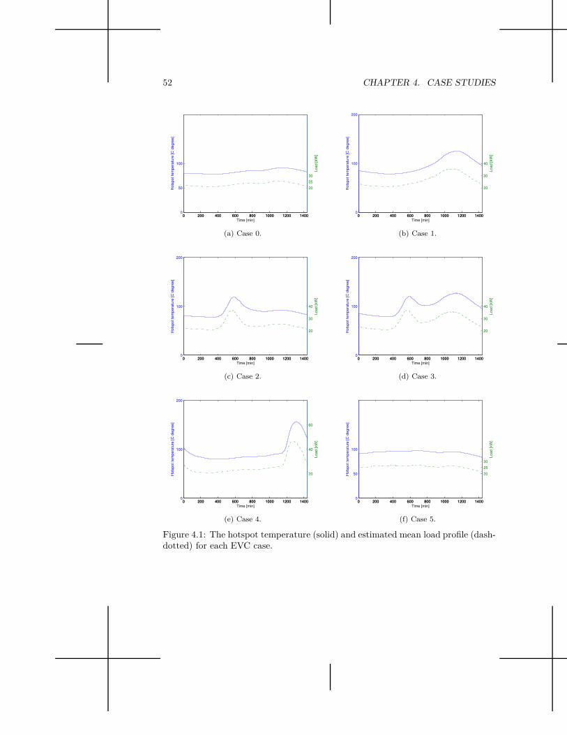
52 CHAPTER 4. CASE STUDIES
0 200 400 600 800 1000 1200 14000
50
100
Ho
tsp
ot
tem
pe
ratu
re [
C d
eg
ree
]
Time [min]0 200 400 600 800 1000 1200 1400
20
25
30
Lo
ad
[kW
]
(a) Case 0.
0 200 400 600 800 1000 1200 14000
100
200
Ho
tsp
ot
tem
pe
ratu
re [
C d
eg
ree
]
Time [min]0 200 400 600 800 1000 1200 1400
20
30
40
Lo
ad
[kW
]
(b) Case 1.
0 200 400 600 800 1000 1200 14000
100
200
Ho
tsp
ot
tem
pe
ratu
re [
C d
eg
ree
]
Time [min]0 200 400 600 800 1000 1200 1400
20
30
40
Lo
ad
[kW
]
(c) Case 2.
0 200 400 600 800 1000 1200 14000
100
200
Ho
tsp
ot
tem
pe
ratu
re [
C d
eg
ree
]
Time [min]0 200 400 600 800 1000 1200 1400
20
30
40
Lo
ad
[kW
]
(d) Case 3.
0 200 400 600 800 1000 1200 14000
100
200
Ho
tsp
ot
tem
pe
ratu
re [
C d
eg
ree
]
Time [min]0 200 400 600 800 1000 1200 1400
20
40
60
Lo
ad
[kW
]
(e) Case 4.
0 200 400 600 800 1000 1200 14000
50
100
Ho
tsp
ot
tem
pe
ratu
re [
C d
eg
ree
]
Time [min]0 200 400 600 800 1000 1200 1400
20
25
30
Lo
ad
[kW
]
(f) Case 5.
Figure 4.1: The hotspot temperature (solid) and estimated mean load profile (dash-dotted) for each EVC case.

4.1. CASE STUDY WITH THE EVC-A MODEL 53
0 200 400 600 800 1000 1200 14000
20
40
60
80
100
Ho
tsp
ot
tem
pe
ratu
re [
C d
eg
ree
]
Time [min]0 200 400 600 800 1000 1200 1400
020406080100L
oss o
f lif
e [
min
]
(a) Case 0.
0 200 400 600 800 1000 1200 14000
20
40
60
80
100
120
140
Ho
tsp
ot
tem
pe
ratu
re [
C d
eg
ree
]
Time [min]0 200 400 600 800 1000 1200 1400
0
200
400
600
800
1000
1200
1400
Lo
ss o
f lif
e [
min
]
(b) Case 1.
0 200 400 600 800 1000 1200 14000
100
200
Ho
tsp
ot
tem
pe
ratu
re [
C d
eg
ree
]
Time [min]0 200 400 600 800 1000 1200 1400
0
200
400
Lo
ss o
f lif
e [
min
]
(c) Case 2.
0 200 400 600 800 1000 1200 14000
100
200
Ho
tsp
ot
tem
pe
ratu
re [
C d
eg
ree
]
Time [min]0 200 400 600 800 1000 1200 1400
0
1000
2000
Lo
ss o
f lif
e [
min
]
(d) Case 3.
0 200 400 600 800 1000 1200 14000
20
40
60
80
100
120
140
160
Ho
tsp
ot
tem
pe
ratu
re [
C d
eg
ree
]
Time [min]0 200 400 600 800 1000 1200 1400
0
1000
2000
3000
4000
5000
6000
7000
8000
Lo
ss o
f lif
e [
min
]
(e) Case 4.
0 200 400 600 800 1000 1200 14000
50
100
Ho
tsp
ot
tem
pe
ratu
re [
C d
eg
ree
]
Time [min]0 200 400 600 800 1000 1200 1400
0
200
400
Lo
ss o
f lif
e [
min
]
(f) Case 5.
Figure 4.2: The hotspot temperature (solid) and the cumulative loss of life (dash-dotted) for each EVC case.
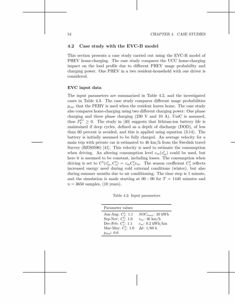
54 CHAPTER 4. CASE STUDIES
4.2 Case study with the EVC-B model
This section presents a case study carried out using the EVC-B model ofPHEV home-charging. The case study compares the UCC home-chargingimpact on the load profile due to different PHEV usage probability andcharging power. One PHEV in a two resident-household with one driver isconsidered.
EVC input data
The input parameters are summarized in Table 4.2, and the investigatedcases in Table 4.3. The case study compares different usage probabilitiespcar that the PEHV is used when the resident leaves home. The case studyalso compares home-charging using two different charging power: One phasecharging and three phase charging (230 V and 10 A). UniC is assumed,thus P t,i
V ≥ 0. The study in [40] suggests that lithium-ion battery life ismaintained if deep cycles, defined as a depth of discharge (DOD), of lessthan 60 percent is avoided, and this is applied using equation (3.14). Thebattery is initially assumed to be fully charged. An average velocity for amain trip with private car is estimated to 46 km/h from the Swedish travelSurvey (RES0596) [41]. This velocity is used to estimate the consumptionwhen driving. An altering consumption level cm(vt
m) could be used, buthere it is assumed to be constant, including losses. The consumption whendriving is set to Ct(vt
m, Cts) = cmCt
svm. The season coefficient Cts reflects
increased energy need during cold external conditions (winter), but alsoduring summer months due to air conditioning. The time step is 1 minute,and the simulation is made starting at 00 : 00 for T = 1440 minutes andn = 3650 samples, (10 years).
Table 4.2: Input parameters
Parameter values
Jun-Aug: Cts: 1.1 SOCmax: 20 kWh
Sep-Nov: Cts: 1.0 vm: 46 km/h
Dec-Feb: Cts: 1.1 cm: 0.2 kWh/km
Mar-May: Cts: 1.0 ∆t: 1/60 h
pdod: 0.6

4.2. CASE STUDY WITH THE EVC-B MODEL 55
Table 4.3: Investigated cases
Case Parameter values
1 pcar: 0.17Cp: 2.3 kW
2 pcar: 0.6Cp: 2.3 kW
3 pcar: 0.17Cp: 6.9 kW
Residential activity data
The transition state probabilities are constant hourly average values basedon time-use data from a Swedish survey covering 431 persons in 103 detachedhouses and 66 apartments [36]. Time use surveys are conducted in manyadditional countries, for example in Finland, France, Germany, Italy, UKand Belgium [42]. The transition state probabilities depend on the form ofhousing and whether it is a weekend or weekday and this is described indetail in [35]. The activities are listed in Table 4.4.
Table 4.4: Set of activities
Code Activity Code Activity
1 Away 6 TV2 Sleeping 7 Computer3 Cooking 8 Audio4 Dishwashing 9 Other5 Washing
Results
Figure 4.3 shows the convergence of the estimate of the mean load with theEVC-B model at 5pm (for P V
1020,j and j = 1, ..., 3650). This indicates thatthe number of samples is enough to determine that the estimate of the mean

56 CHAPTER 4. CASE STUDIES
value has converged, ensuring that the simulation is made for a sufficientnumber of samples.
0 500 1000 1500 2000 2500 3000 35000
0.2
0.4
0.6
0.8
1
1.2
Sample (j)
Pow
er
(kW
)
Figure 4.3: Convergency of the estimate of the mean load at 5pm, P V1020,j , Case 1
In Figures 4.4-4.6 the resulting estimated expected EVC load profilesfor the three cases are shown. In Case 1 and Case 3, the PHEV consumesin average 2.4 kWh/day. With an electricity consumption of 0.2 kWh/kmthese cases correspond to in average 12 km electrically driven distance/day.In Case 2 the PHEV consumes in average 7.5 kWh/day, corresponding toaround 38 km electrically driven distance. For comparison, the daily drivendistance by private car is in the county of Stockholm in average 22 km andin the county of Halland in average 36 km according to [41]. The estimatesof the expected load profiles show how UCC charging at home most likelyoccurs in the afternoon.
In Figures 4.7, 4.8 and 4.9 show the standard deviation estimates for theexpected household load and the increased standard deviation estimates forwhen the PHEV is included. The standard deviation estimate in Figure 4.9is not entirely smooth and this is related to two reasons: The set of datamay be too limited to give a smooth estimate, why a larger set of real worlddata would give a smoother result. The second reason could be that thetransition probabilities in the data set are the same for all minutes in eachhour, but changes in each hour shift. This may be mitigated by interpolatingthe transition probabilities. The Figures 4.7, 4.8 and 4.9 show a stochasticbehavior that varies less in the morning than in midday and evening hours.This is related to the electricity-dependent activities and their dependencyof individuals to be at home.
In Case 1 the EVC represents around 30% of the total load during loadpeak and a share of around 20% of the daily electricity use. In Case 2 the
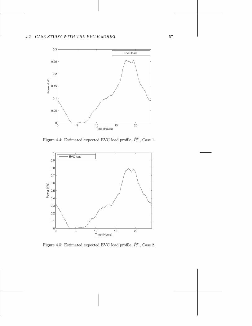
4.2. CASE STUDY WITH THE EVC-B MODEL 57
0 5 10 15 200
0.05
0.1
0.15
0.2
0.25
0.3
Time (Hours)
Pow
er
(kW
)
EVC load
Figure 4.4: Estimated expected EVC load profile, P Vi , Case 1.
0 5 10 15 200
0.1
0.2
0.3
0.4
0.5
0.6
0.7
0.8
0.9
1
Time (Hours)
Pow
er
(kW
)
EVC load
Figure 4.5: Estimated expected EVC load profile, P Vi , Case 2.
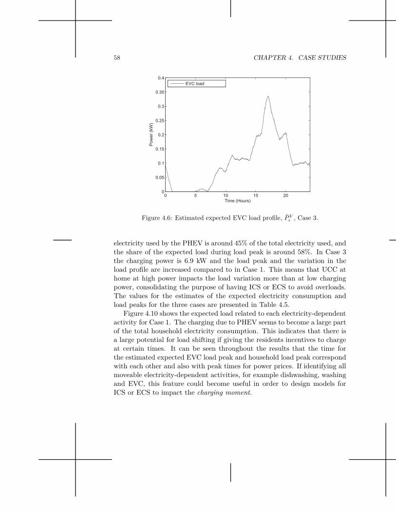
58 CHAPTER 4. CASE STUDIES
0 5 10 15 200
0.05
0.1
0.15
0.2
0.25
0.3
0.35
0.4
Time (Hours)
Pow
er
(kW
)
EVC load
Figure 4.6: Estimated expected EVC load profile, P Vi , Case 3.
electricity used by the PHEV is around 45% of the total electricity used, andthe share of the expected load during load peak is around 58%. In Case 3the charging power is 6.9 kW and the load peak and the variation in theload profile are increased compared to in Case 1. This means that UCC athome at high power impacts the load variation more than at low chargingpower, consolidating the purpose of having ICS or ECS to avoid overloads.The values for the estimates of the expected electricity consumption andload peaks for the three cases are presented in Table 4.5.
Figure 4.10 shows the expected load related to each electricity-dependentactivity for Case 1. The charging due to PHEV seems to become a large partof the total household electricity consumption. This indicates that there isa large potential for load shifting if giving the residents incentives to chargeat certain times. It can be seen throughout the results that the time forthe estimated expected EVC load peak and household load peak correspondwith each other and also with peak times for power prices. If identifying allmoveable electricity-dependent activities, for example dishwashing, washingand EVC, this feature could become useful in order to design models forICS or ECS to impact the charging moment.
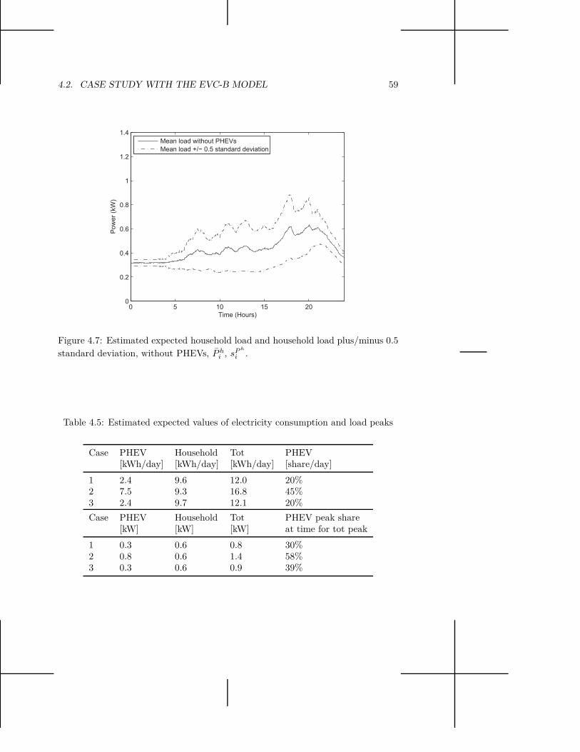
4.2. CASE STUDY WITH THE EVC-B MODEL 59
0 5 10 15 200
0.2
0.4
0.6
0.8
1
1.2
1.4
Time (Hours)
Pow
er
(kW
)
Mean load without PHEVs
Mean load +/− 0.5 standard deviation
Figure 4.7: Estimated expected household load and household load plus/minus 0.5
standard deviation, without PHEVs, P hi , sP h
i .
Table 4.5: Estimated expected values of electricity consumption and load peaks
Case PHEV Household Tot PHEV[kWh/day] [kWh/day] [kWh/day] [share/day]
1 2.4 9.6 12.0 20%2 7.5 9.3 16.8 45%3 2.4 9.7 12.1 20%
Case PHEV Household Tot PHEV peak share[kW] [kW] [kW] at time for tot peak
1 0.3 0.6 0.8 30%2 0.8 0.6 1.4 58%3 0.3 0.6 0.9 39%
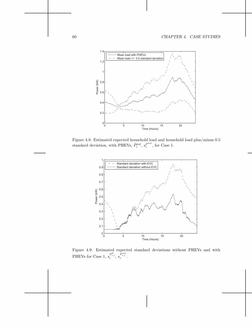
60 CHAPTER 4. CASE STUDIES
0 5 10 15 200
0.2
0.4
0.6
0.8
1
1.2
1.4
Time (Hours)
Pow
er
(kW
)
Mean load with PHEVs
Mean load +/− 0.5 standard deviation
Figure 4.8: Estimated expected household load and household load plus/minus 0.5standard deviation, with PHEVs, P tot
i , sP tot
i , for Case 1.
0 5 10 15 200
0.1
0.2
0.3
0.4
0.5
0.6
0.7
0.8
0.9
1
Time (Hours)
Pow
er
(kW
)
Standard deviation with EVC
Standard deviation without EVC
Figure 4.9: Estimated expected standard deviations without PHEVs and with
PHEVs for Case 1, sP h
i,j
i , sP tot
i,j
i .
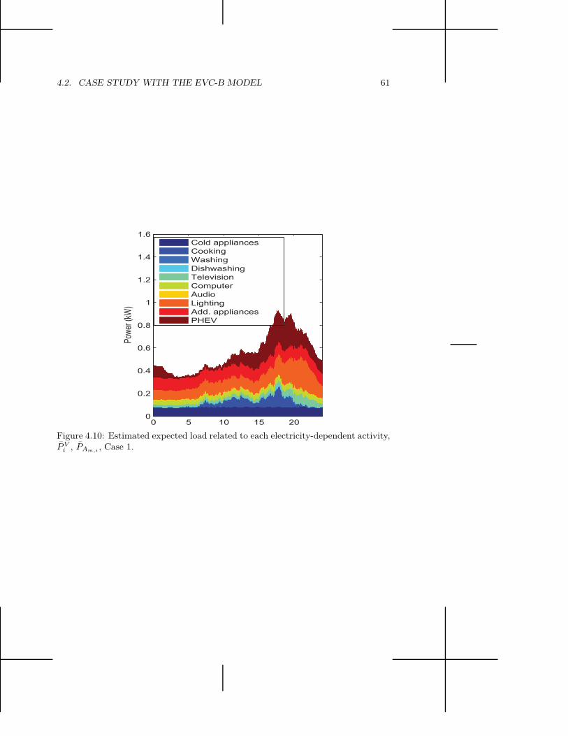
4.2. CASE STUDY WITH THE EVC-B MODEL 61
0 5 10 15 200
0.2
0.4
0.6
0.8
1
1.2
1.4
1.6
Pow
er (k
W)
Cold appliances
Cooking
Washing
Dishwashing
Television
Computer
Audio
Lighting
Add. appliances
PHEV
Figure 4.10: Estimated expected load related to each electricity-dependent activity,P V
i , PAm,i, Case 1.
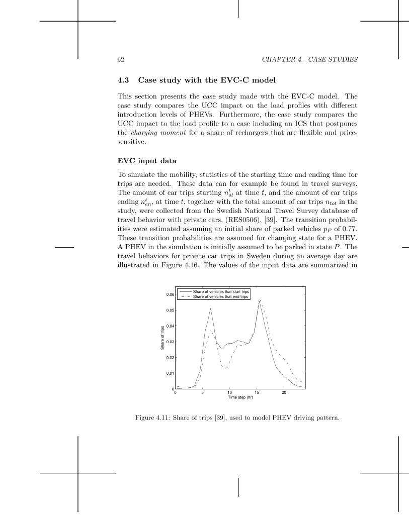
62 CHAPTER 4. CASE STUDIES
4.3 Case study with the EVC-C model
This section presents the case study made with the EVC-C model. Thecase study compares the UCC impact on the load profiles with differentintroduction levels of PHEVs. Furthermore, the case study compares theUCC impact to the load profile to a case including an ICS that postponesthe charging moment for a share of rechargers that are flexible and price-sensitive.
EVC input data
To simulate the mobility, statistics of the starting time and ending time fortrips are needed. These data can for example be found in travel surveys.The amount of car trips starting nt
st at time t, and the amount of car tripsending nt
en, at time t, together with the total amount of car trips ntot in thestudy, were collected from the Swedish National Travel Survey database oftravel behavior with private cars, (RES0506), [39]. The transition probabil-ities were estimated assuming an initial share of parked vehicles pP of 0.77.These transition probabilities are assumed for changing state for a PHEV.A PHEV in the simulation is initially assumed to be parked in state P . Thetravel behaviors for private car trips in Sweden during an average day areillustrated in Figure 4.16. The values of the input data are summarized in
0 5 10 15 200
0.01
0.02
0.03
0.04
0.05
0.06
Time step (hr)
Share
of tr
ips
Share of vehicles that start trips
Share of vehicles that end trips
Figure 4.11: Share of trips [39], used to model PHEV driving pattern.

4.3. CASE STUDY WITH THE EVC-C MODEL 63
Table 4.6. The overall consumption comes from data of a Monday in Jan-uary in Sweden [43]. In [39] the total number of private cars in the Swedishcar fleet is estimated to be around 4.3 millions. Shares of the total numberof cars are used in the case study in order to illustrate the impact of differentintroduction levels of PHEVs.
Table 4.6: Input data
Symbol Value Symbol Value
pP 0.77 n 10000 samplesntot 17006 Pc 2.3 kWSOCi
max 25 kWh F imin 0.6
vm 46 km/h N 29 dayscm 0.174 kWh/km T 24 hoursCm 8 kWh/h ki ∈ U(−0.05, 0.05)∆t 0.5 pF 0.8
Charging price variation
The charging price Etp is assumed to follow price signals from the electricity
spot price variations, with forecasts performed one day before. However,this does not mean that the price Et
p necessarily is the total electricity pricefor charging. It only indicates that the EVC could be set to react to thespot price variations. An EVC price is set by estimating the mean pricecurve pt and standard deviation st
p for N daily price curves pt. The EVCprice Et
p at time t is assumed to be normally distributed according to:
Etp ∈ N(pt, st
p/√
N) (4.1)
The charging price Etp is sampled using N = 29 days of spot price data from
Nordpool in February 2012.
Results
A test run with this set up, presented in Figure 4.12 (a), shows the twostates: Parked, P represented by 1 and Driving, D by 2, and the transitionbetween these states of UCC for a PHEV recharger i during a day. InFigure 4.12 (b) the SOC due to driving and charging the PHEV i can be
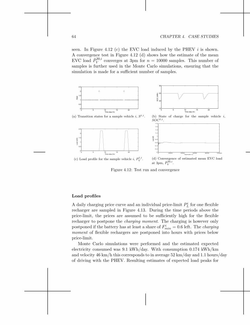
64 CHAPTER 4. CASE STUDIES
seen. In Figure 4.12 (c) the EVC load induced by the PHEV i is shown.A convergence test in Figure 4.12 (d) shows how the estimate of the meanEVC load P 30,i
V converges at 3pm for n = 10000 samples. This number ofsamples is further used in the Monte Carlo simulations, ensuring that thesimulation is made for a sufficient number of samples.
0 5 10 15 200
0.5
1
1.5
2
2.5
Time step (hr)
Sta
te
(a) Transition states for a sample vehicle i, St,i.
0 5 10 15 2015
20
25
30
Time step (hr)
SO
C (
kW
h)
(b) State of charge for the sample vehicle i,SOCt,i.
0 5 10 15 200
0.5
1
1.5
2
2.5
Time step (hr)
Load (
kW
)
(c) Load profile for the sample vehicle i, Pt,i
V.
0 2000 4000 6000 8000 100000
0.2
0.4
0.6
0.8
1
1.2
1.4
1.6
1.8
Sample (i) L
oad
(kW
)
(d) Convergence of estimated mean EVC load
at 3pm, P30,i
V.
Figure 4.12: Test run and convergence
Load profiles
A daily charging price curve and an individual price-limit P iL for one flexible
recharger are sampled in Figure 4.13. During the time periods above theprice-limit, the prices are assumed to be sufficiently high for the flexiblerecharger to postpone the charging moment. The charging is however onlypostponed if the battery has at least a share of F i
min = 0.6 left. The chargingmoment of flexible rechargers are postponed into hours with prices belowprice-limit.
Monte Carlo simulations were performed and the estimated expectedelectricity consumed was 9.1 kWh/day. With consumption 0.174 kWh/kmand velocity 46 km/h this corresponds to in average 52 km/day and 1.1 hours/dayof driving with the PHEV. Resulting estimates of expected load peaks for
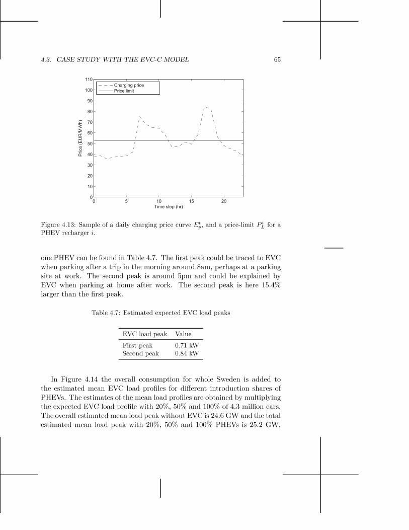
4.3. CASE STUDY WITH THE EVC-C MODEL 65
0 5 10 15 200
10
20
30
40
50
60
70
80
90
100
110
Time step (hr)
Price (
EU
R/M
Wh)
Charging price
Price limit
Figure 4.13: Sample of a daily charging price curve Etp, and a price-limit P i
L for aPHEV recharger i.
one PHEV can be found in Table 4.7. The first peak could be traced to EVCwhen parking after a trip in the morning around 8am, perhaps at a parkingsite at work. The second peak is around 5pm and could be explained byEVC when parking at home after work. The second peak is here 15.4%larger than the first peak.
Table 4.7: Estimated expected EVC load peaks
EVC load peak Value
First peak 0.71 kWSecond peak 0.84 kW
In Figure 4.14 the overall consumption for whole Sweden is added tothe estimated mean EVC load profiles for different introduction shares ofPHEVs. The estimates of the mean load profiles are obtained by multiplyingthe expected EVC load profile with 20%, 50% and 100% of 4.3 million cars.The overall estimated mean load peak without EVC is 24.6 GW and the totalestimated mean load peak with 20%, 50% and 100% PHEVs is 25.2 GW,
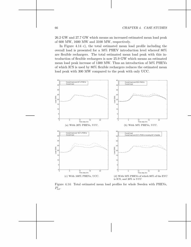
66 CHAPTER 4. CASE STUDIES
26.2 GW and 27.7 GW which means an increased estimated mean load peakof 600 MW, 1600 MW and 3100 MW, respectively.
In Figure 4.14 c), the total estimated mean load profile including theoverall load is presented for a 50% PHEV introduction level whereof 80%are flexible rechargers. The total estimated mean load peak with this in-troduction of flexible rechargers is now 25.9 GW which means an estimatedmean load peak increase of 1300 MW. Thus an introduction of 50% PHEVsof which ICS is used by 80% flexible rechargers reduces the estimated meanload peak with 300 MW compared to the peak with only UCC.
0 5 10 15 200
5
10
15
20
25
30
35
40
Time step (hr)
Load (
GW
)
Overall load and 20 % PHEVs
Overall load
(a) With 20% PHEVs, UCC.
0 5 10 15 200
5
10
15
20
25
30
35
40
Time step (hr)
Load (
GW
)
Overall load and 50% PHEVs
Overall load
(b) With 50% PHEVs, UCC.
0 5 10 15 200
5
10
15
20
25
30
35
40
Time step (hr)
Load (
GW
)
Overall load and 100 % PHEVs
Overall load
(c) With 100% PHEVs, UCC.
0 5 10 15 200
5
10
15
20
25
30
35
40
Time step (hr)
Load (
GW
)
Overall load
Overall load and 50 % PHEVs including 80 % flexible
(d) With 50% PHEVs of which 80% of the EVCis ICS, and 20% is UCC
Figure 4.14: Total estimated mean load profiles for whole Sweden with PHEVs,P t
tot.
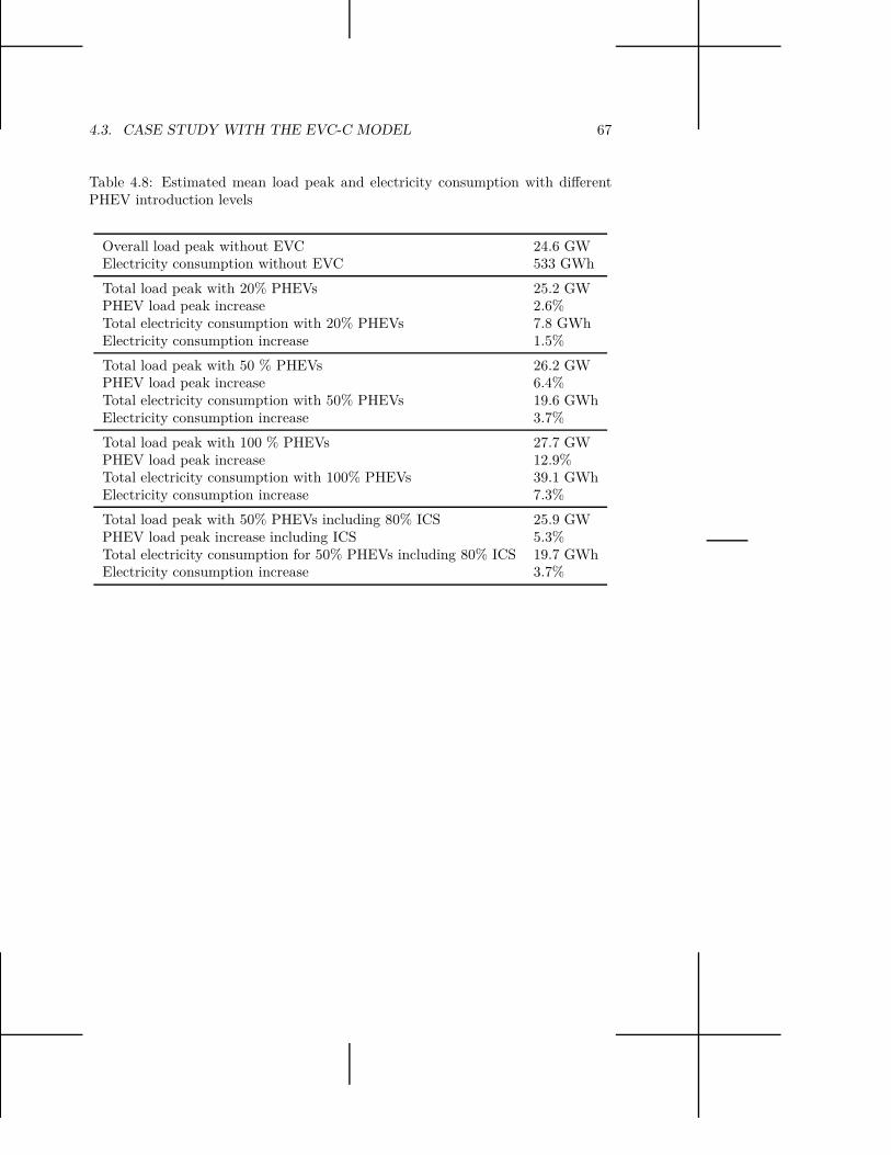
4.3. CASE STUDY WITH THE EVC-C MODEL 67
Table 4.8: Estimated mean load peak and electricity consumption with differentPHEV introduction levels
Overall load peak without EVC 24.6 GWElectricity consumption without EVC 533 GWh
Total load peak with 20% PHEVs 25.2 GWPHEV load peak increase 2.6%Total electricity consumption with 20% PHEVs 7.8 GWhElectricity consumption increase 1.5%
Total load peak with 50 % PHEVs 26.2 GWPHEV load peak increase 6.4%Total electricity consumption with 50% PHEVs 19.6 GWhElectricity consumption increase 3.7%
Total load peak with 100 % PHEVs 27.7 GWPHEV load peak increase 12.9%Total electricity consumption with 100% PHEVs 39.1 GWhElectricity consumption increase 7.3%
Total load peak with 50% PHEVs including 80% ICS 25.9 GWPHEV load peak increase including ICS 5.3%Total electricity consumption for 50% PHEVs including 80% ICS 19.7 GWhElectricity consumption increase 3.7%
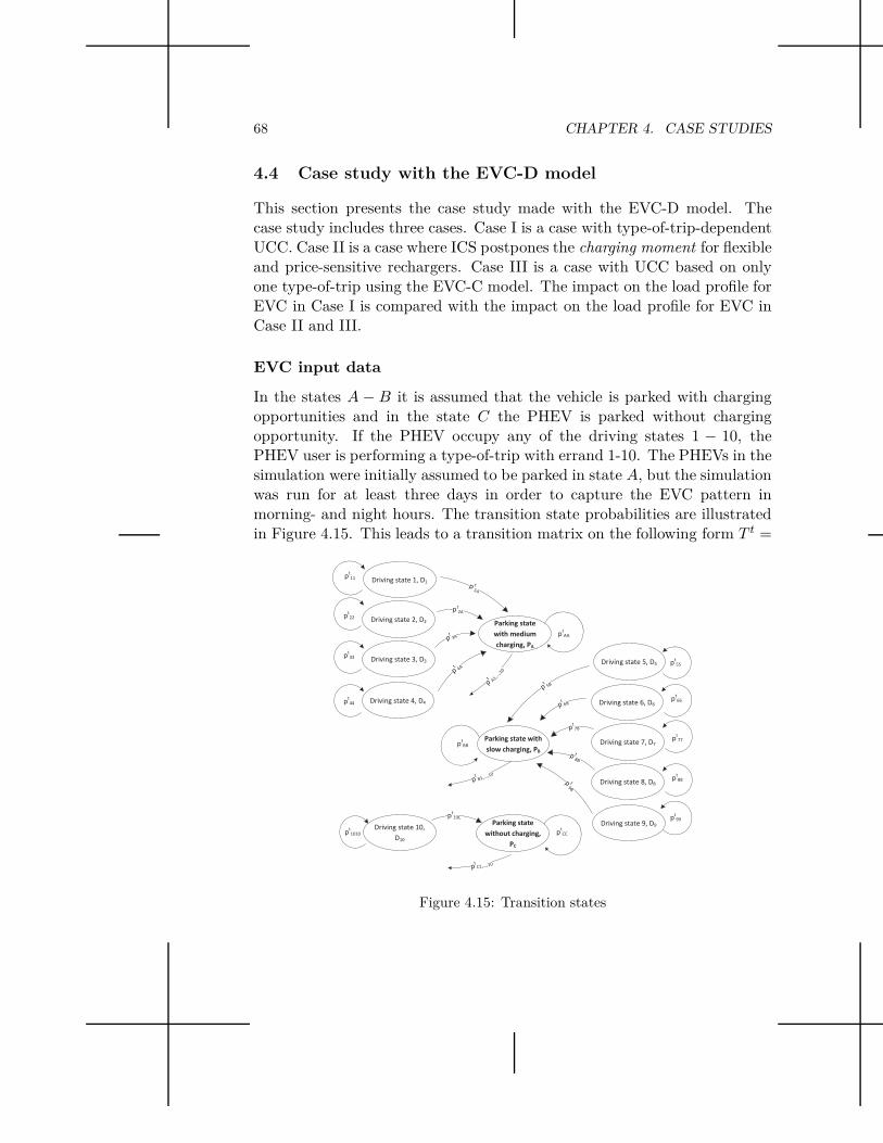
68 CHAPTER 4. CASE STUDIES
4.4 Case study with the EVC-D model
This section presents the case study made with the EVC-D model. Thecase study includes three cases. Case I is a case with type-of-trip-dependentUCC. Case II is a case where ICS postpones the charging moment for flexibleand price-sensitive rechargers. Case III is a case with UCC based on onlyone type-of-trip using the EVC-C model. The impact on the load profile forEVC in Case I is compared with the impact on the load profile for EVC inCase II and III.
EVC input data
In the states A − B it is assumed that the vehicle is parked with chargingopportunities and in the state C the PHEV is parked without chargingopportunity. If the PHEV occupy any of the driving states 1 − 10, thePHEV user is performing a type-of-trip with errand 1-10. The PHEVs in thesimulation were initially assumed to be parked in state A, but the simulationwas run for at least three days in order to capture the EVC pattern inmorning- and night hours. The transition state probabilities are illustratedin Figure 4.15. This leads to a transition matrix on the following form T t =
Parking state with
slow charging, PB
Driving state 5, D5
Parking state
with medium
charging, PA
ptAA
pt55
Parking state
without charging,
PC
ptBB
ptCC
p t1A
Driving state 1, D1p
t11
Driving state 2, D2p
t22
Driving state 3, D3p
t33
pt
A1,...,1
0
Driving state 4, D4pt44
Driving state 10,
D10
pt1010
Driving state 6, D6p
t66
Driving state 7, D7p
t77
Driving state 8, D8p
t88
Driving state 9, D9
pt99
pt
B1,...,10
pt
C1,...,10
pt2A
pt
3A
pt
5B
pt
6B
pt7B
pt
4A
p t8B
p t9B
pt10C
Figure 4.15: Transition states

4.4. CASE STUDY WITH THE EVC-D MODEL 69
ptAA 0 0 p
tA1 p
tA2 p
tA3 p
tA4 p
tA5 p
tA6 p
tA7 p
tA8 p
tA9 p
tA10
0 ptBB 0 p
tB1 p
tB2 p
tB3 p
tB4 p
tB5 p
tB6 p
tB7 p
tB8 p
tB9 p
tB10
0 0 ptCC p
tC1 p
tC2 p
tC3 p
tC4 p
tC5 p
tC6 p
tC7 p
tC8 p
tC9 p
tC10
pt1A 0 0 p
t11 0 0 0 0 0 0 0 0 0
pt2A 0 0 0 p
t22 0 0 0 0 0 0 0 0
pt3A 0 0 0 0 p
t33 0 0 0 0 0 0 0
pt4A 0 0 0 0 0 p
t44 0 0 0 0 0 0
0 pt5B 0 0 0 0 0 p
t55 0 0 0 0 0
0 pt6B 0 0 0 0 0 0 p
t66 0 0 0 0
0 pt7B 0 0 0 0 0 0 0 p
t77 0 0 0
0 pt8B 0 0 0 0 0 0 0 0 p
t88 0 0
0 pt9B 0 0 0 0 0 0 0 0 0 p
t99 0
0 0 pt10C 0 0 0 0 0 0 0 0 0 p
t1010
,
(4.2)
were t ∈ τ .
Transition probability data
Assuming that car travel behavior remain the same as of today, private cartravel data can for example be found in the Swedish National travel survey(RES0506) [39]. The RES0506 database covers detailed travel informationfrom the period of 1th October 2005 to 30th September 2006 of respondents’movements, mode of transport, errand of the journey, starting and endingtimes. In the database information can also be found concerning gender,age, employment, holding of driving licences and the households’ number ofcars as well as housing form. National Travel Surveys are also conductedin many countries in addition to Sweden, for example in US [44], UK [45],Germany [46], Denmark [47], The Netherlands [48], New Zealand [49] andSouth Africa [50].
Data for the amount of a type-of-trip z starting, nt,zst or ending nt,z
en , attime t for average weekdays and weekend days were obtained from RES0506.The transition probabilities estimated based on these travel data are as-sumed concerning changing from one state to another for a PHEV. Thedata were primarily hourly, whilst for the simulations they were interpo-lated into ∆t = 0.25 hourly steps. The share of these type-of-trips’ startingand ending times for a weekday are illustrated in Figures 4.17 and 4.16.

70 CHAPTER 4. CASE STUDIES
2 4 6 8 10 12 14 16 18 20 22 240
0.02
0.04
0.06
0.08
0.1
0.12
Time step (hr)
Share
of
sta
rtin
g t
rips
1
2
3
4
5
6
7
8
9
10
Figure 4.16: Share of starting vehicle trips a weekday used to model PHEVs drivingpattern with type-of-trip defined in Table 4.9, [39].
5 10 15 200
0.02
0.04
0.06
0.08
0.1
0.12
Time step (hr)
Share
of
endin
g t
rips
1
2
3
4
5
6
7
8
9
10
Figure 4.17: Share of ending vehicle trips a weekday used to model PHEVs drivingpattern with type-of-trip defined in Table 4.9, [39].
Type-of-trip parametrization
The car trips average weekdays and weekend days were divided into groupsaccording to type-of-trips performed in the RES0506 database. The re-

4.4. CASE STUDY WITH THE EVC-D MODEL 71
sult of this grouping is presented in Table. 4.9 where ’Other errand’ is thesum of type-of-trips listed in Table 4.10. The number of car travel data-points were 1’882’587, and in order to estimate the transition probabilitiesthe initial amount n0
Dz performing type-of-trip z, were set to n0D1=112’470,
n0D2,3,4=56’233, n0
D5,6,8,9=3’601, n0D7=10’803, n0
D10=99’239.
Table 4.9: States related to type-of-trip and charging opportunity
Parking state, x Charging opportunity Symbol
A Medium charging pA
B Slow charging pB
C No charging pC
Driving state, z Type-of-trip Symbol Parking mode
1 Work commute p1 A2 Study commute p2 A3 Groceries shopping p3 A4 Other shopping p4 A
5 Medical or health care p5 B6 Post or bank errand p6 B7 Visit family or friends p7 B8 Visit restaurant or cafe p8 B9 Entertainment or culture p9 B
10 Other errand p10 C
In the RES0506 database average values of the velocity on average cartrips are found to be in the interval 35-46 km/h. The velocity vm is assumedto be type-of-trip dependent. Furthermore, the electricity consumption cm,and the second fuel consumption gm, are assumed to be type-of-trip andvelocity-dependent. The type-of-trips are categorized in three groups, m =1, 2, 3 and it is assumed that each type-of-trip belongs to one these. Thegrouping is made based on the characteristic of the type-of-trip which isassumed to impact the velocity and consumption due to external conditionssuch as for example driving in a rural or urban area. The grouping is madeconsidering the errand, and commuting type-of-trips 1, 2, and groceriesshopping type-of-trip 3 are set to belong to m = 1. These type-of-trips areassumed to be similar to each other and performed with a relatively lowmean velocity and consumption.

72 CHAPTER 4. CASE STUDIES
Table 4.10: Type-of-trips included in Other errand
Type-of-trip
Errand at work Other serviceErrand while studying Other private errandTicket booking Other vacationPick up child Other recreational activityExercise and recreation Other restaurant, cafe visitDrive or pick up person Other post or bank relatedParticipation in childs’ activity Other drive or pick up personClub activities and religion Other unknown errandOther hobbies
The type-of-trips 5, 6, 8, and 9 are trips related to bank, post, medicalcare, restaurant or entertainment errands, and these are here set to belongto m = 2. These type-of-trips are assumed to be similar to each other andperformed in an urban environment with a slightly higher mean velocity andconsumption than for m = 1. The type-of-trips 4, 7 and 10 are trips relatedto other shopping, visiting family and friends or other errands, and theseare here set to belong to m = 3. These type-of-trips are assumed to includemore highway driving implying a higher mean velocity and consumption.
It is thus assumed that the consumption level C1 while driving holdsfor type-of-trips 1, 2, 3, C2 is for type-of-trips 5, 6, 8, 9, and C3 is fortype-of-trips 4, 7, 10. The discharging efficiency ηdc, is set to 86%. Theelectricity consumption cm or second fuel consumption gm, while driving isassumed to be related to three different velocities v1,2,3 sampled from normaldistributions with 20% standard deviation from mean: v1 ∈ N(30, 30 · 0.2),v2 ∈ N(40, 40 · 0.2) and v3 ∈ N(50, 50 · 0.2) km/h. These velocities are usedto find the distance driven and the electricity or second fuel used in each∆t.
Depending on the driving cycle, the consumption of an EV is in [51] esti-mated to lie in between 0.12 kWh/km and 0.20 kWh/km. Average consump-tions c1,2,3 are here sampled from normal distributions with 10% standarddeviation from mean: c1 ∈ N(0.19, 0.19 · 0.1), c2 ∈ N(0.20, 0.20 · 0.1) andc3 ∈ N(0.25, 0.25 · 0.1) kWh/km. This results in three electricity consump-tions levels Cm = cm · vm kWh/h when driving.
The second fuel is assumed to be gasoline with consumption g1,2,3 sam-

4.4. CASE STUDY WITH THE EVC-D MODEL 73
pled from sampled from normal distributions with 10% standard devia-tion from mean: g1 ∈ N(0.05, 0.05 · 0.1), g2 ∈ N(0.06, 0.06 · 0.1), g3 ∈N(0.07, 0.07 · 0.1) liters/km, respectively. This results in three consump-tions gm · vm liters/h when driving using the second fuel. For Case IIIconstant values of c2, v2 and g2 are used.
Charging behavior data
The individual battery size SOCimax, and the individual tank size SOT i
max
are assumed to be uniformly distributed in the intervals [18, 22] kWh and[45, 55] liter, respectively. For the individual flexible rechargers in Case II theminimum fraction of the battery levels is sampled from a normal distributionF i
min ∈ N(0.4, 0.2). The slow charging Pc1, is set to 2.3 kW, for one-phasecharging at (230 V, 10 A), the medium charging Pc2 to 3.7 kW for (230 V,16 A) and the fast charging Pc3 to 50 kW. The charging efficiency ηc, is set to97%. The added load is the overall electricity consumption in Swedish areaSE3 based on data for 21 weekdays in February, 12 Saturdays in January-March and 12 Sundays in January-March 2012 in Sweden [43]. The totalSwedish area SE3 includes counties such as Gotland, Stockholm, Söderman-lands, Uppsala, Värmland, Västmanland, Örebro, Östergötland and partsof Jönköping, Halland , Kalmar, Västra Götaland, Gävleborg and Dalarna.The total number of people with a car and a driver’s licence in these countiesare found to be around 2.382 millions, [41] why this number is used for Ntot
in order to illustrate a maximum impact of PHEVs. The time step length isset to ∆t = 0.25 hours, and the time period simulated is one week, T = 168.The time period is simulated for n = 1000 samples.
Charging price data
The charging price is assumed to be normally distributed with mean andstandard deviation estimated from the spot price. The EVC price is sampledusing N = 91 days of spot price data from Nordpool in January-Mars 2012.A daily EVC price pt is sampled from N(spt, sspt/
√N) where ¯spt is the
estimated mean spot price and sspt is the estimated spot price standarddeviation. The variable charging price Et
p is set by adding H = 0.1 e/kWhto the sampled EVC price pt and also a fixed charging cost Ec for each slowand medium charging event, of 1 e, and for each fast charging event a fixedcost EF c of 2 e. The individual variation in the price-limit is allowed tovary with 17 % less than the mean price Ep, during weekdays and 1% duringweekend days, set by k1,i ∈ U(0.17, 0.17×2), ∈ U(0.01, 0.01×2). The second
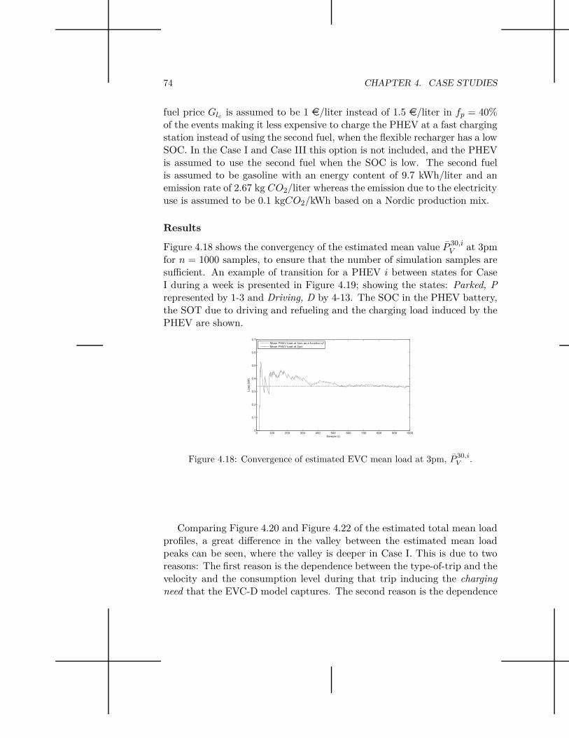
74 CHAPTER 4. CASE STUDIES
fuel price Glc is assumed to be 1 e/liter instead of 1.5 e/liter in fp = 40%of the events making it less expensive to charge the PHEV at a fast chargingstation instead of using the second fuel, when the flexible recharger has a lowSOC. In the Case I and Case III this option is not included, and the PHEVis assumed to use the second fuel when the SOC is low. The second fuelis assumed to be gasoline with an energy content of 9.7 kWh/liter and anemission rate of 2.67 kg CO2/liter whereas the emission due to the electricityuse is assumed to be 0.1 kgCO2/kWh based on a Nordic production mix.
Results
Figure 4.18 shows the convergency of the estimated mean value P 30,iV at 3pm
for n = 1000 samples, to ensure that the number of simulation samples aresufficient. An example of transition for a PHEV i between states for CaseI during a week is presented in Figure 4.19; showing the states: Parked, Prepresented by 1-3 and Driving, D by 4-13. The SOC in the PHEV battery,the SOT due to driving and refueling and the charging load induced by thePHEV are shown.
0 100 200 300 400 500 600 700 800 900 10000
0.1
0.2
0.3
0.4
0.5
0.6
0.7
Sample (i)
Load (
kW
)
Mean PHEV load at 3pm as a function of i
Mean PHEV load at 3pm
Figure 4.18: Convergence of estimated EVC mean load at 3pm, P 30,iV .
Comparing Figure 4.20 and Figure 4.22 of the estimated total mean loadprofiles, a great difference in the valley between the estimated mean loadpeaks can be seen, where the valley is deeper in Case I. This is due to tworeasons: The first reason is the dependence between the type-of-trip and thevelocity and the consumption level during that trip inducing the chargingneed that the EVC-D model captures. The second reason is the dependence
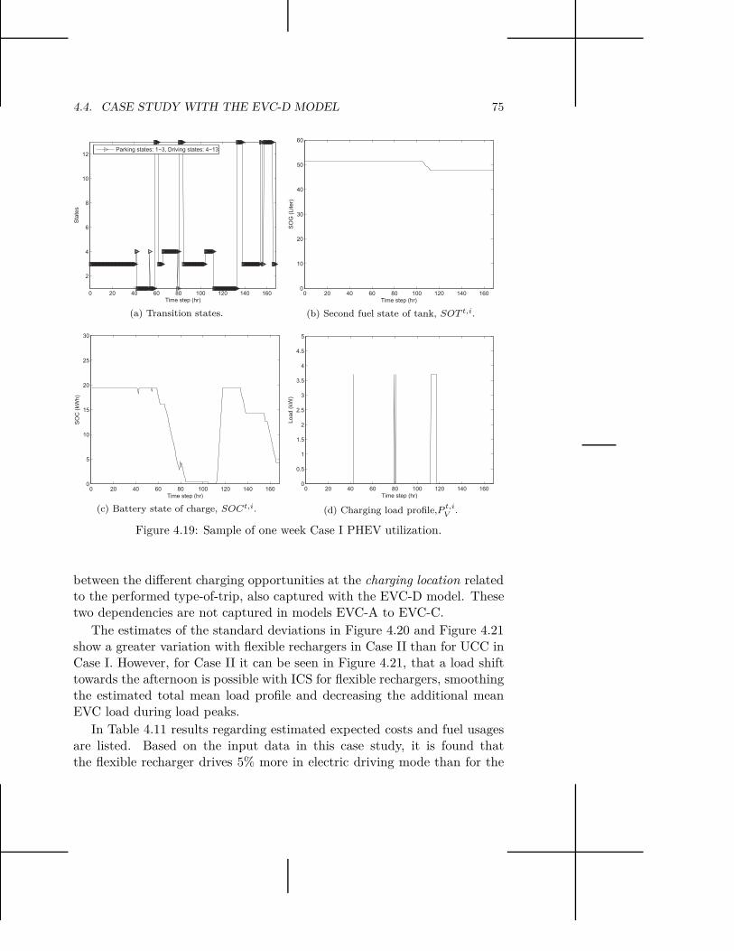
4.4. CASE STUDY WITH THE EVC-D MODEL 75
0 20 40 60 80 100 120 140 160
2
4
6
8
10
12
Sta
tes
Time step (hr)
Parking states: 1−3, Driving states: 4−13
(a) Transition states.
0 20 40 60 80 100 120 140 1600
10
20
30
40
50
60
Time step (hr)
SO
G (
Liter)
(b) Second fuel state of tank, SOT t,i.
0 20 40 60 80 100 120 140 1600
5
10
15
20
25
30
Time step (hr)
SO
C (
kW
h)
(c) Battery state of charge, SOCt,i.
0 20 40 60 80 100 120 140 1600
0.5
1
1.5
2
2.5
3
3.5
4
4.5
5
Time step (hr)
Load (
kW
)
(d) Charging load profile,P t,i
V.
Figure 4.19: Sample of one week Case I PHEV utilization.
between the different charging opportunities at the charging location relatedto the performed type-of-trip, also captured with the EVC-D model. Thesetwo dependencies are not captured in models EVC-A to EVC-C.
The estimates of the standard deviations in Figure 4.20 and Figure 4.21show a greater variation with flexible rechargers in Case II than for UCC inCase I. However, for Case II it can be seen in Figure 4.21, that a load shifttowards the afternoon is possible with ICS for flexible rechargers, smoothingthe estimated total mean load profile and decreasing the additional meanEVC load during load peaks.
In Table 4.11 results regarding estimated expected costs and fuel usagesare listed. Based on the input data in this case study, it is found thatthe flexible recharger drives 5% more in electric driving mode than for the
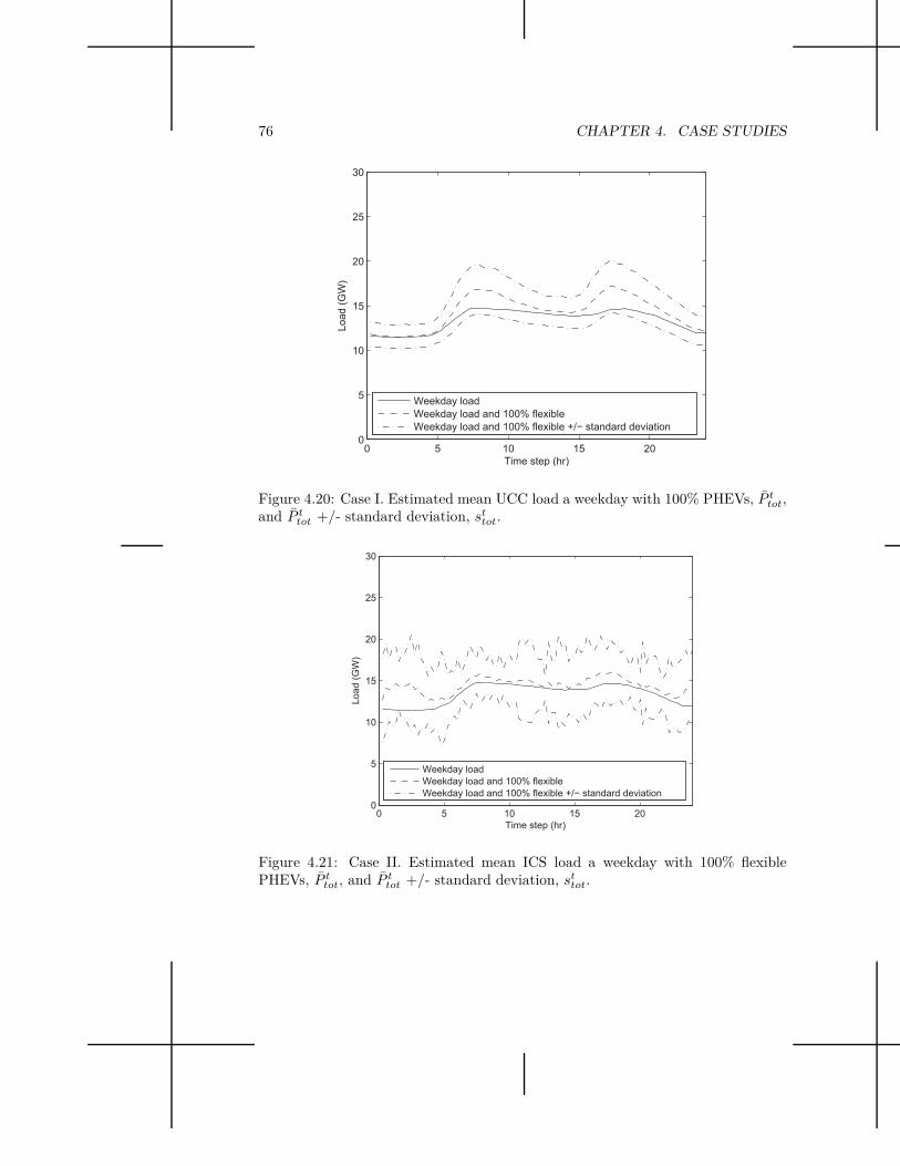
76 CHAPTER 4. CASE STUDIES
0 5 10 15 200
5
10
15
20
25
30
Time step (hr)
Load (
GW
)
Weekday load
Weekday load and 100% flexible
Weekday load and 100% flexible +/ standard deviation
Figure 4.20: Case I. Estimated mean UCC load a weekday with 100% PHEVs, P ttot,
and P ttot +/- standard deviation, st
tot.
0 5 10 15 200
5
10
15
20
25
30
Time step (hr)
Load (
GW
)
Weekday load
Weekday load and 100% flexible
Weekday load and 100% flexible +/ standard deviation
Figure 4.21: Case II. Estimated mean ICS load a weekday with 100% flexiblePHEVs, P t
tot, and P ttot +/- standard deviation, st
tot.
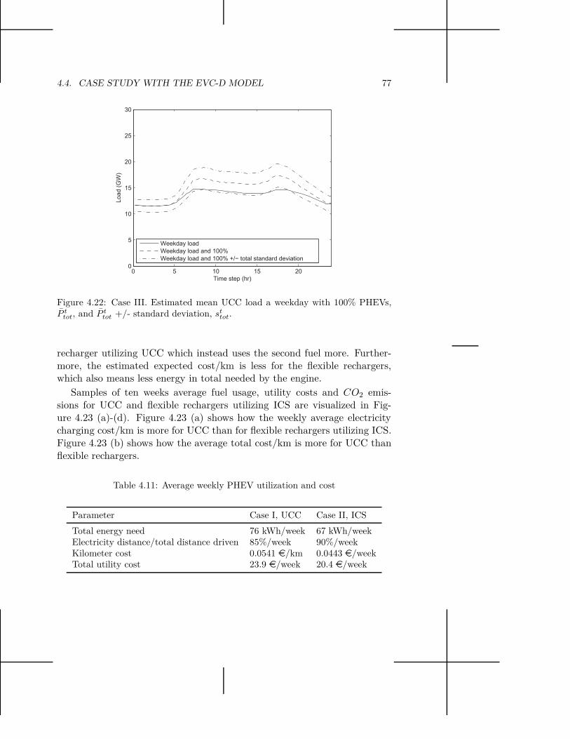
4.4. CASE STUDY WITH THE EVC-D MODEL 77
0 5 10 15 200
5
10
15
20
25
30
Time step (hr)
Load (
GW
)
Weekday load
Weekday load and 100%
Weekday load and 100% +/ total standard deviation
Figure 4.22: Case III. Estimated mean UCC load a weekday with 100% PHEVs,P t
tot, and P ttot +/- standard deviation, st
tot.
recharger utilizing UCC which instead uses the second fuel more. Further-more, the estimated expected cost/km is less for the flexible rechargers,which also means less energy in total needed by the engine.
Samples of ten weeks average fuel usage, utility costs and CO2 emis-sions for UCC and flexible rechargers utilizing ICS are visualized in Fig-ure 4.23 (a)-(d). Figure 4.23 (a) shows how the weekly average electricitycharging cost/km is more for UCC than for flexible rechargers utilizing ICS.Figure 4.23 (b) shows how the average total cost/km is more for UCC thanflexible rechargers.
Table 4.11: Average weekly PHEV utilization and cost
Parameter Case I, UCC Case II, ICS
Total energy need 76 kWh/week 67 kWh/weekElectricity distance/total distance driven 85%/week 90%/weekKilometer cost 0.0541 e/km 0.0443 e/weekTotal utility cost 23.9 e/week 20.4 e/week

78 CHAPTER 4. CASE STUDIES
250 300 350 400 4500.04
0.045
0.05
0.055
0.06
0.065
0.07
0.075
0.08
Average weekly electric distance driven (km)
Avera
ge w
ee
kly
ele
ctr
icity
kilo
mete
r cost
(EU
R/k
m) Inflexible
Flexible
(a) Electric charging cost.
250 300 350 400 450 500 5500
0.01
0.02
0.03
0.04
0.05
0.06
0.07
0.08
0.09
Average weekly total distance driven (km)
Avera
ge w
eekly
tota
l kilo
mete
r cost
(EU
R/k
m)
Inflexible
Flexible
(b) Kilometer cost.
0.04 0.045 0.05 0.055 0.06 0.065 0.07 0.075 0.080
0.5
1
1.5
2
2.5
3
Average weekly second fuel distance driven (km)
Avera
ge w
eekly
second f
uel kilo
mete
r cost
(EU
R/k
m) Inflexible
Flexible
(c) Second fuel cost.
4 6 8 10 12 14 16 18 20 22 240.04
0.042
0.044
0.046
0.048
0.05
0.052
0.054
0.056
0.058
0.06
Avera
ge w
ee
kly
tota
lkilo
me
ter
cost
(EU
R/k
m)
Total weekly emissions (Kg CO2)
Inflexible
Flexible
(d) CO2 emissions.
Figure 4.23: Case I with UCC compared to Case II with ICS, average weekly PHEVutilization, emissions and costs.

4.5. CASE STUDY SUMMARY 79
4.5 Case study summary
The case studies were carried out to show the value of the models developedin this licentiate thesis. The case studies show the EVC impact on load pro-files due to only considering home-charging, and due to including chargingopportunities at several parking locations. Furthermore, the impact on loadprofiles when using developed models with greater level of detail, includingthe type-of-trips performed and type-of-trip-dependent consumption leveland charging opportunity, and also due including charging flexibility areshown. All case studies consider UniC.
The case study with the EVC-A model evaluates the impact on loadprofiles considering the charging location to be at home or at a commutingparking site, based on UCC or ECS. The case study with the EVC-B modelevaluates UCC impact on the load profile considering the charging locationto be only at home. The case study with the EVC-C model evaluates theimpact due to UCC and ICS with flexible rechargers performing one type-of-trip with the charging location allowed to be during parking event at anylocation, and UCC or an ICS due to price sensitivity. The case study withthe EVC-D model considers UCC based on various types-of-trips with re-lated charging opportunities, and UniC, or an ICS with flexible rechargersdue to price sensitivity. The EVC-D model takes into account chargingopportunities, velocities and consumption levels related to the type-of-trip.With the EVC-D model it is also possible to capture parking events withoutcharging opportunity related to the type-of-trip. The ICS in EVC-D model,in comparison to the ICS in the EVC-C model, also takes into account thechoice between fast charging and driving on a second fuel due to price sensi-tivity. The case study with the EVC-D model also considers CO2 emissions,distance driven with the second fuel, and electricity and utility costs whichmay be compared for UCC and ICS.
The model performances and the model considerations of the chargingoption and driving consumption levels are summarized in Table 4.12. Thesimulation time for the EVC-B model is longer than the simulation timefor the EVC-A model due to the generation of the underlying syntheticactivities. In the EVC-C model and the EVC-D model the key factors aretreated as dependent on each other, and in EVC-D they are also time-andtype-of-trip-dependent. The simulation time for the EVC-D model becomeslonger than for the EVC-C model due to this higher level of detail in thetravel modeling. The conditions added to the EVC-C model and the EVC-Dmodel in order to model ICS yet adds some simulation time.
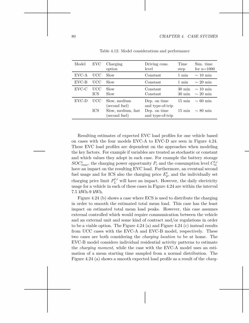
80 CHAPTER 4. CASE STUDIES
Table 4.12: Model considerations and performance
Model EVC Charging Driving cons. Time Sim. timeoption level step for n=1000
EVC-A UCC Slow Constant 1 min ∼ 10 min
EVC-B UCC Slow Constant 1 min ∼ 20 min
EVC-C UCC Slow Constant 30 min ∼ 10 minICS Slow Constant 30 min ∼ 20 min
EVC-D UCC Slow, medium Dep. on time 15 min ∼ 60 min(second fuel) and type-of-trip
ICS Slow, medium, fast Dep. on time 15 min ∼ 80 min(second fuel) and type-of-trip
Resulting estimates of expected EVC load profiles for one vehicle basedon cases with the four models EVC-A to EVC-D are seen in Figure 4.24.These EVC load profiles are dependent on the approaches when modelingthe key factors. For example if variables are treated as stochastic or constantand which values they adopt in each case. For example the battery storageSOCi
max, the charging power opportunity Pc and the consumption level Ct,im
have an impact on the resulting EVC load. Furthermore, an eventual secondfuel usage and for ICS also the charging price Et
p, and the individually set
charging price limit P t,iL will have an impact. However, the daily electricity
usage for a vehicle in each of these cases in Figure 4.24 are within the interval7.5 kWh-9 kWh.
Figure 4.24 (b) shows a case where ECS is used to distribute the chargingin order to smooth the estimated total mean load. This case has the leastimpact on estimated total mean load peaks. However, this case assumesexternal controlled which would require communication between the vehicleand an external unit and some kind of contract and/or regulations in orderto be a viable option. The Figure 4.24 (a) and Figure 4.24 (c) instead resultsfrom UCC cases with the EVC-A and EVC-B model, respectively. Thesetwo cases are both considering the charging location to be at home. TheEVC-B model considers individual residential activity patterns to estimatethe charging moment, while the case with the EVC-A model uses an esti-mation of a mean starting time sampled from a normal distribution. TheFigure 4.24 (a) shows a smooth expected load profile as a result of the charg-

4.5. CASE STUDY SUMMARY 81
ing moment estimation. The case study with the EVC-B model results in aless smooth expected load profile, which can be seen in in Figure 4.24 (c),as a result of the underlying individual activity patterns. The estimated ex-pected load peak for this case becomes less than the peak in Figure 4.24 (a)when the resulting EVC pattern is distributed in a longer time period forthe case using the EVC-B model.
Both Figure 4.24 (a) and Figure 4.24 (c) show cases where chargingat any other location than at home is neglected. Figure 4.24 (d) insteadshows an EVC pattern based on the possibility to charge the battery afterevery trip. This case, with the EVC-C model, in addition to charging athome, captures the daily travel patterns better than the previous cases.However, this case is based on an assumption that available outlets exitsat any parking site. In Figure 4.24 (e) and Figure 4.24 (f) the resultingestimate of the expected EVC load in an UCC case and an ICS case usingthe EVC-D model, respectively are shown. These two cases with the EVC-D model also capture daily travel patterns, and in addition also chargingopportunities at parking events related to the type-of-trip. In the UCC casesusing the EVC-C model and the EVC-D model these daily travel patternsand assumptions result in two daily expected load peaks instead of one asin the previous cases in Figure 4.24 (a) and Figure 4.24 (c). The timing forthese two load peaks coincides with the timing for peak power prices whichshould be useful to consider if wanting to design incentives for ICS and ECS.
In Figure 4.24 (e) there is a deeper valley in the middle of the day com-pared to the estimate of the expected load profile in Figure 4.24 (d). This isdue to the dependence between the different charging opportunities relatedto the performed type-of-trip, captured with the EVC-D model. The valleyis also due to the dependence between the type-of-trip, the velocity and theconsumption level which together induce a time-dependent charging needthat the EVC-D model also captures. In Figure 4.24 (f) the ICS case usingthe EVC-D model is shown. The estimate of the expected EVC load profilewith ICS shows a greater load variation due to the flexible rechargers, thanfor the UCC. This increased variation is related to the stochastic EVC be-havior that arises due to the charging-price limit that is sampled for eachindividual. With flexible rechargers it can also be seen in Figure 4.24 (f),that a load shift towards night hours is possible with ICS. This load shiftwould smooth the total expected mean load profile and decrease the addi-tional expected EVC load at load peaks.

82 CHAPTER 4. CASE STUDIES
0 5 10 15 200
0.5
1
1.5
2
2.5
Ele
ctr
ic v
eh
icle
lo
ad
[kW
]
Time of day [Hours]
(a) EVC-A, UCC.
0 5 10 15 200
0.5
1
1.5
2
2.5
Ele
ctr
ic v
eh
icle
lo
ad
[kW
]
Time of day [Hours]
(b) EVC-A, ECS.
0 5 10 15 200
0.1
0.2
0.3
0.4
0.5
0.6
0.7
0.8
0.9
1
Time (Hours)
Pow
er
(kW
)
EVC load
(c) EVC-B, UCC.
0 5 10 15 200
0.5
1
1.5
2
2.5
Time step (hr)L
oa
d (
kW
)
Mean EVC load
Standard deviation
(d) EVC-C, UCC.
0 5 10 15 200
0.5
1
1.5
2
2.5
3
Time step (hr)
Lo
ad
(kW
)
Mean EVC load
Standard deviation
(e) EVC-D, UCC.
0 5 10 15 200
0.5
1
1.5
2
2.5
3
3.5
4
4.5
5
Time step (hr)
Lo
ad
(kW
)
Mean EVC load
Standard deviation
(f) EVC-D, ICS.
Figure 4.24: Estimated expected EVC load of UniC for one vehicle with the intro-duced models P t
V , and also P tV + st
V for EVC-C and EVC-D.
4.6 Concluding remarks
By using the EVC models it is possible to estimate time-dependent expectedEVC load profiles based on EV utilization and induced charging needs. It isalso possible to estimate expected EVC load profiles for flexible rechargersdue to charging price sensitivity with the models EVC-C and EVC-D. Withthe model EVC-D is is also possible to estimate the mead cost of the elec-

4.6. CONCLUDING REMARKS 83
tricity usage and compare it to the estimated cost of a second fuel for UCCand flexible recharging utilizing ICS. The flexibility to postpone the charg-ing moment due to charging price sensitivity in models EVC-C and EVC-Daffect the load profiles by smoothing the overall average load profiles. How-ever, with the ICS in these two models the variation for the estimate of theEVC load standard deviation increases compared to for the modeled UCC.
The results from the case studies with the EVC models show how theindividual vehicle utilization induces a charging need and creates a charg-ing behavior that will impact the overall power system. The results allowfor a quantification of the time-dependent charging load impact, accountingfor the UCC load variation that is brought to the system. This gives gridcompanies (DSOs) opportunities to estimate anticipated needs for invest-ments or upgrades in the grid infrastructure. An opportunity also arises toestimate needs for incentives in order to impact the charging location, thecharging need and the charging moment of future EVC.
The case study with the EVC-C model shows that with an introduction ofvehicles that are allowed to charge their battery at any parking event, thiswould create two load peaks, related to the travel and parking behavior.Based on the case study it is seen that if 50% of the Swedish vehicle fleetwas electricity-driven the estimated mean load peak in Sweden would beincreased with 1300 MW. If ICS is used by 80 % flexible rechargers in thiscase, the estimated mean load peak is reduced with 300 MW compared towith only UCC.
In the case study with the EVC-D model the type-of-trip is taken intoconsideration and also charging opportunities of medium charging powerrelated to commuting trips which is the largest share of the type-of-tripsperformed. This results in a deeper load valley in the middle of the day andgreater load peaks than in the case with the EVC-C model. The peaks arerelated to charging when arriving to work and charging when arriving homeafter work. If 50% of the whole Swedish vehicle fleet was electricity-drivenhaving an EVC pattern based on the travel pattern and charging opportu-nities in the case study with the EVC-D model, this creates an estimatedmean load peak increase of around 2200 MW. This is 900 MW more thanthe estimated mean load peak increase resulting from the UCC case modeledwith the EVC-C model of 1300 MW. With the ICS in the EVC-D model theestimated mean load peak is reduced with around 400 MW, into an increaseof around 1800 MW. For comparison, if 50% of the Swedish vehicle fleet waselectricity-driven and consuming 6 TWh/year, this corresponds to a mean

84 CHAPTER 4. CASE STUDIES
consumption of around 685 MW.These quantities show the importance of taking into account travel pat-
terns and related charging opportunities when considering a large-scale EVintroduction. The estimated mean EVC load peaks may be reduced furtherwith smarter approaches of ICS and/or ECS.
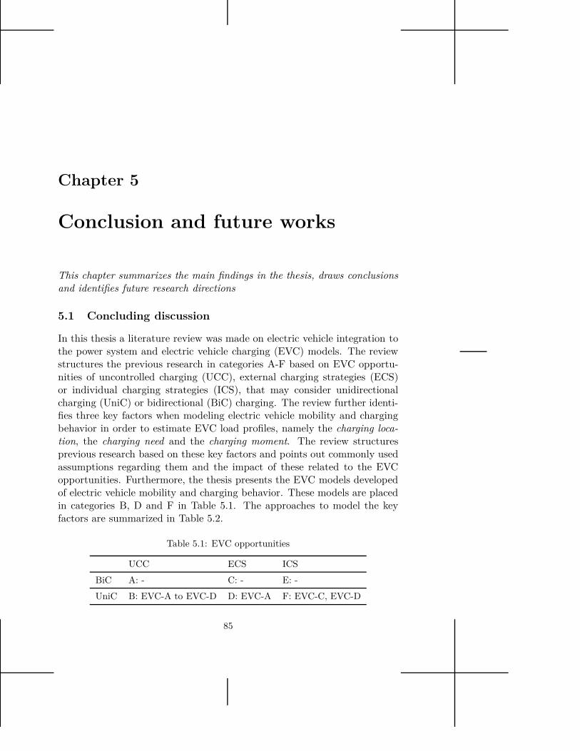
Chapter 5
Conclusion and future works
This chapter summarizes the main findings in the thesis, draws conclusionsand identifies future research directions
5.1 Concluding discussion
In this thesis a literature review was made on electric vehicle integration tothe power system and electric vehicle charging (EVC) models. The reviewstructures the previous research in categories A-F based on EVC opportu-nities of uncontrolled charging (UCC), external charging strategies (ECS)or individual charging strategies (ICS), that may consider unidirectionalcharging (UniC) or bidirectional (BiC) charging. The review further identi-fies three key factors when modeling electric vehicle mobility and chargingbehavior in order to estimate EVC load profiles, namely the charging loca-tion, the charging need and the charging moment. The review structuresprevious research based on these key factors and points out commonly usedassumptions regarding them and the impact of these related to the EVCopportunities. Furthermore, the thesis presents the EVC models developedof electric vehicle mobility and charging behavior. These models are placedin categories B, D and F in Table 5.1. The approaches to model the keyfactors are summarized in Table 5.2.
Table 5.1: EVC opportunities
UCC ECS ICS
BiC A: - C: - E: -
UniC B: EVC-A to EVC-D D: EVC-A F: EVC-C, EVC-D
85

86 CHAPTER 5. CONCLUSION AND FUTURE WORKS
The impact on the load profile was investigated with the EVC-A model,simulating different EVC cases. The EVC load impact on transformerhotspot temperature and loss of life was investigated. The results indi-cate that UCC could lead to increased load peaks, effecting the transformerloss of life negatively, when exponential aging behavior occur during loadpeaks. Furthermore, the results imply that with an ECS that distributesthe charging moment would reduce the risk for overloads.
The EVC-B model was developed for PHEV home-charging. With themodel it is possible to simulate the residential total expected load profileboth due to PHEV charging and other electricity-dependent activities per-formed in a household. Both the expected total load profile as well as thevariation in the load profile can be obtained with the model, and the resultsfrom the case study show that with UCC the charging mostly occurs in theafternoon. In Case 1 in the case study with the EVC-B model, the PHEVrepresents around one third of the total expected load during the load peakand around a fifth of the total expected electric energy used/day. The modelmakes it possible to differentiate and compare the electricity use due to UCCwith other residential electricity-dependent activities, indicating a potentialfor load shifting.
The EVC-C model of UCC was developed estimating the charging needfrom travel patterns. With the model it is possible to estimate expectedcharging load profiles depending on the introduction level and charging flex-ibility, allowing the charging location to be at a parking location after anytrip performed. Results from the case study with the model, based onSwedish conditions with travel statistics from the Swedish National TravelSurvey (RES0506) for private cars, show how an introduction of PHEVsin the car park may affect the overall load and load peaks due to charg-ing patterns. Simulations with the model also show with ICS how flexiblerechargers may mitigate the overall load peak increase, shifting the chargingmoment into hours with lower demand, indicating an opportunity for PHEVbatteries to act as flexible loads to reduce load peaks.
The EVC-D model of UCC model was developed which treats all threekey factors as dependent variables. With the EVC-D model it is possibleto simulate detailed PHEV mobility behavior due to the type-of-trip andrelated charging opportunities. The EVC impact on the overall load profileis estimated by introducing the charging location to be at several parkingsites after type-of-trips with different consumption levels. The model isgeneral and was in a case study applied to the Swedish National Travel

5.1. CONCLUDING DISCUSSION 87
Survey (RES0506) for private cars to simulate the estimated mean electricityuse and load profiles with many PHEVs in the vehicle fleet. In the casestudy the proposed model that takes into account different type-of-trips withrelated consumption levels and charging opportunities was compared to theEVC-C model that only takes into account one type-of-trip. The resultfrom the case study with the EVC-D model also show that ICS with flexiblePHEV rechargers that postpone their charging moments, the load peaksmay be mitigated, indicating a potential for load shifting with flexible PHEVrechargers together with an opportunity of reducing PHEV utilization costs,second fuel usage and CO2 emissions.
The case studies with the EVC-C and EVC-D models show that EVCmay create two load peaks related to the travel and parking behavior. Basedon the case study with the EVC-C it is seen that if 50% of the Swedish ve-hicle fleet was electricity-driven the estimated mean load peak in Swedenwould be increased with 1300 MW. If ICS is used by 80 % flexible recharg-ers, the estimated mean load peak is reduced with 300 MW compared tothe estimated mean load peak with only UCC. In the case study with theEVC-D model the type-of-trip is taken into consideration and also chargingopportunities of medium charging power related to commuting trips which isthe largest share of the type-of-trips performed. This creates a deeper loadvalley in the middle of the day and greater estimated mean load peaks thanin the case with the EVC-C model. The peaks are related to charging whenarriving to work and charging when arriving home after work. If 50% ofthe whole Swedish vehicle fleet was electricity-driven with an EVC patternbased on the travel pattern and charging opportunities in the case studywith the EVC-D model, this creates an estimated mean load peak increaseof around 2200 MW. This is 900 MW more than the estimated mean loadpeak increase resulting from the UCC case modeled with the EVC-C modelof 1300 MW. With the ICS in the EVC-D model the estimated mean loadpeak is reduced with around 400 MW, into an increase of around 1800 MW.For comparison, if 50% of the Swedish vehicle fleet was electricity-drivenand consuming 6 TWh/year, this would correspond to a mean consumptionof around 685 MW.
These quantities show the importance of taking into account travel pat-terns and related charging opportunities when considering a large-scale EVintroduction. The modeled estimated mean EVC load peaks may be reducedfurther with smarter approaches of ICS and/or ECS.
It may be concluded that the level of details concerning the approach
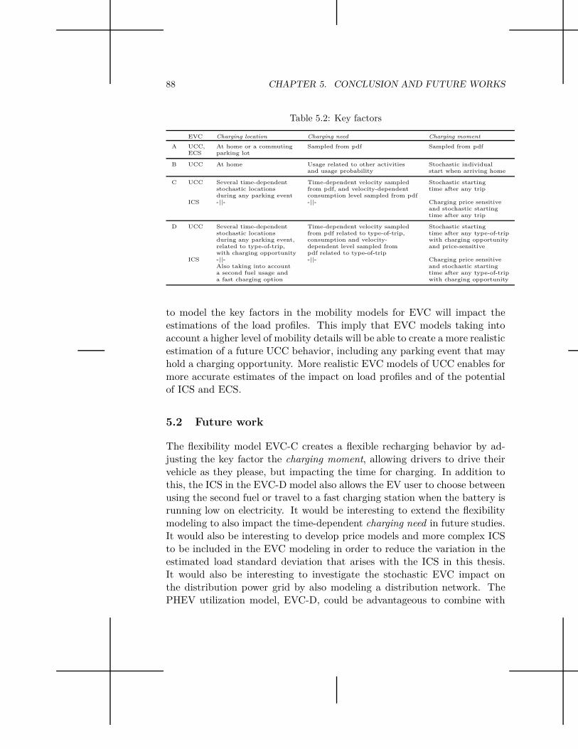
88 CHAPTER 5. CONCLUSION AND FUTURE WORKS
Table 5.2: Key factors
EVC Charging location Charging need Charging moment
A UCC, At home or a commuting Sampled from pdf Sampled from pdfECS parking lot
B UCC At home Usage related to other activities Stochastic individualand usage probability start when arriving home
C UCC Several time-dependent Time-dependent velocity sampled Stochastic startingstochastic locations from pdf, and velocity-dependent time after any tripduring any parking event consumption level sampled from pdf
ICS -||- -||- Charging price sensitiveand stochastic startingtime after any trip
D UCC Several time-dependent Time-dependent velocity sampled Stochastic startingstochastic locations from pdf related to type-of-trip, time after any type-of-tripduring any parking event, consumption and velocity- with charging opportunityrelated to type-of-trip, dependent level sampled from and price-sensitivewith charging opportunity pdf related to type-of-trip
ICS -||- -||- Charging price sensitiveAlso taking into account and stochastic startinga second fuel usage and time after any type-of-tripa fast charging option with charging opportunity
to model the key factors in the mobility models for EVC will impact theestimations of the load profiles. This imply that EVC models taking intoaccount a higher level of mobility details will be able to create a more realisticestimation of a future UCC behavior, including any parking event that mayhold a charging opportunity. More realistic EVC models of UCC enables formore accurate estimates of the impact on load profiles and of the potentialof ICS and ECS.
5.2 Future work
The flexibility model EVC-C creates a flexible recharging behavior by ad-justing the key factor the charging moment, allowing drivers to drive theirvehicle as they please, but impacting the time for charging. In addition tothis, the ICS in the EVC-D model also allows the EV user to choose betweenusing the second fuel or travel to a fast charging station when the battery isrunning low on electricity. It would be interesting to extend the flexibilitymodeling to also impact the time-dependent charging need in future studies.It would also be interesting to develop price models and more complex ICSto be included in the EVC modeling in order to reduce the variation in theestimated load standard deviation that arises with the ICS in this thesis.It would also be interesting to investigate the stochastic EVC impact onthe distribution power grid by also modeling a distribution network. ThePHEV utilization model, EVC-D, could be advantageous to combine with

5.2. FUTURE WORK 89
models of geographical charging location, to find expected EVC load profilesin different areas. It would be interesting to combine the EVC and mobilitymodels with models of the power grid including active and reactive powerflows, especially when considering BiC. For example it would be interestingto study the opportunity of using and V2G in order to provide ancillaryservices to the power grid, or in a different case implement vehicle-to-home(V2H) in order to provide back-up power to the household.
It could also be valuable to combine EVC models of the electric vehiclebatteries as stochastic flexible loads with forecast models of wind and solarpower production in order to find the potential to reduce future power pro-duction variations with a large-scale introduction of renewable and variablepower production.
Moreover, the models could be used in case studies for load shaving anddemand side management by identifying movable activities. The PHEVhome-charging model, EVC-B, could be used to investigate for which activ-ities, and how, load shifting would impact the household load profile andhow load peaks may be reduced with ECS and/or ICS.


Bibliography
[1] “Directive 2009/33/EC of the European Parliament and of theCouncil of 23 April 2009 on the promotion of clean and energy ef-ficient road transport vehicles,” http://eur-lex.europa.eu/LexUriServ/LexUriServ.do?uri=OJ:L:2009:120:0005:0012:en:pdf, official Journal ofthe European Union.
[2] H. Sköldberg, E. Löfblad, D. Holmström, and B. Ry-dén, “Fossil-fuel independent transport 2030, (in Swedish),www.elforsk.se/programomraden/omv–system/rapporter/,” Tech.Rep.
[3] H. Bandhold, J. Carragher Wallner, M. Lindgren, and S. Bergman,“Plug in road 2020,” Elforsk 09:40, Tech. Rep., 2009. [Online].Available: www.elforsk.se
[4] O. Larsson, “Ladda för nya marknader, elbilens konsekvenser förelnät, elproduktionen och servicestrukturer, (in Swedish),” VINNOVAAnalys, Tech. Rep., 2010. [Online]. Available: www.vinnova.se
[5] T. Markel, M. Kuss, and P. Denholm, “Communication and control ofelectric drive vehicles supporting renewables,” in IEEE Vehicle Powerand Propulsion Conference, VPPC, 2009.
[6] “Electricity consumption statistics for sweden,” http://www.svk.se/energimarknaden/el/Statistik/Elstatistik-for-hela-Sverige/.
[7] J. Tomić and W. Kempton, “Using fleets of electric-drive vehicles forgrid support,” Journal of Power Sources, vol. 168, pp. 459 – 468, 2007.
[8] W. Kempton and J. Tomić, “Vehicles-to-grid power implemantation:From stabilizing the grid to supporting large-scale renewable energy,”Journal of Power Sources, vol. 144, pp. 280 – 294, 2005.
91

92 BIBLIOGRAPHY
[9] S. Han, S. Han, and K. Sezaki, “Development of an optimal vehicle-to-grid aggregator for frequency regulation,” IEEE Transactions on smartgrid, vol. 1, pp. 65 – 72, 2010.
[10] S.-L. Andersson, A. K. Elofsson, M. D. Galus, L. Göransson, S. Karls-son, F. Johnsson, and G. Andersson, “Plug-in Hybrid Electric Vehiclesas Control Power: Case studies of Sweden and Germany.” Energy Pol-icy, vol. 38, pp. 2751 – 2762, 2010.
[11] A. S. Masoum, S. Deliami, P. S. Moses, M. A. S. Masoum, and A. Abu-Siada, “Smart load management of plug-in electric vehicles in distribu-tion and residential networks with charging stations for peak shavingand loss minimisation considering voltage regulation,” IET Generation,Transmission and Distribution, vol. 5, pp. 877–888, 2010.
[12] J. A. Peças Lopes, F. J. Soares, and P. M. Rocha Almeida, “Integrationof electric vehicles in the electric power system,” Proceedings of theIEEE, vol. 99, pp. 168–183, 2011.
[13] N. Rotering and M. Ilic, “Optimal charge control of plug-in hybridelectric vehicles in deregulated electricity markets,” IEEE Transactionson Power Systems, vol. 26, pp. 1021–1029, 2011.
[14] Y. Cao, S. Tang, C. Li, P. Zhang, Y. Tan, Z. Zhang, and J. Li, “Anoptimized EV charging model considering TOU price and SOC curve,”IEEE Transactions on Smart Grid, vol. 3, pp. 388–393, 2012.
[15] P. Richardson, D. Flynn, and A. Keane, “Optimal charging of electricvehicles in low-voltage distribution systems,” IEEE Transactions onPower Systems, vol. 27, pp. 268–279, 2012.
[16] C. Clement-Nyns, E. Haesen, and J. Driesen, “The impact of chargingplug-in hybrid electric vehicles on a residential distribution grid,” IEEETransactions on Power Systems, vol. 25, pp. 371–380, 2010.
[17] K. Qian, C. Zhou, M. Allan, and Y. Yuan, “Modeling load demand dueto EV battery charging in distribution grid,” IEEE Transactions onPower Systems, vol. 26, pp. 802–810, 2011.
[18] S. Shahidinejad, S. Filizadeh, and E. Bibeau, “Profile of charging loadon the grid due to plug-in vehicles,” IEEE Transactions on Smart Grid,vol. 3, pp. 135–141, 2012.
BIBLIOGRAPHY 93
[19] D. Steen, L. A. Tuan, O. Carlson, and L. Bertling, “Assessment ofelectric vehicle charging scenarios based on demographical data,” IEEETransactions on Smart Grid, vol. 3, pp. 1457–1468, 2012.
[20] A. S. Masoum, S. Deliami, P. S. Moses, M. A. S. Masoum, and A. Abu-Siada, “Smart load management of plug-in electric vehicles in distribu-tion and residential networks with charging stations for peak shavingand loss minimisation considering voltage regualtion,” IET Generation,Transmission and Distribution, vol. 5, pp. 877–888, 2010.
[21] S. Shao, M. Pipattanasomporn, and S. Rahman, “Demand response asa load shaping tool in an intelligent grid with electric vehicles,” IEEETransactions on Smart Grid, vol. 2, pp. 624–631, 2011.
[22] D. S. Callaway and I. A. Hiskens, “Achieving controllability of electricloads,” Proceedings of the IEEE, vol. 99, pp. 184–199, 2011.
[23] D. Dallinger, D. Krampe, and M. Wietschel, “Vehicle-to-grid regulationreserves base on a dynamic simulation of mobility behavior,” IEEETransactions on Smart Grid, vol. 2, pp. 302–313, 2011.
[24] L. P. Fernández, T. Gómez San Román, R. Cossent, C. M. Domingo,and P. Frías, “Assessment of the impact of plug-in electric vehicles ondistribution networks,” IEEE Transactions on Power Systems, vol. 26,pp. 206–213, 2011.
[25] T.-K. Lee, B. Adornato, and Z. S. Filipe, “Synthesis of real-world driv-ing cycles and their use for estimating PHEV energy consumption andcharging opportunities: Case study for Midwest/U.S.” IEEE Transac-tions on Vehicular Technology, vol. 60, pp. 4153–4163, 2011.
[26] Z. Darabi and F. Mehdi, “Aggregated impact of plug-in hybrid electricvehicles on electricity demand profile,” IEEE Transactions on Sustain-able Energy, vol. 2, pp. 501–508, 2011.
[27] F. J. Soares, J. A. Peças Lopes, P. M. Rocha Almeida, C. L. Moreira,and L. Seca, “A stochastic model to simulate electric vehicles motionand quantify the energy required from the grid,” in 17th Power SystemsComputation Conference, 2011.
[28] A. Ashtari, E. Bibeau, S. Shahidinejad, and T. Molinski, “Pev chargingprofile predictioin and analysis based on vehicle usage data,” IEEETransactions on Smart Grid, vol. 3, pp. 341–350, 2012.

94 BIBLIOGRAPHY
[29] G. Li and Z. X.-P. and, “Modeling of plug-in hybrid electric vehiclecharging demand in probabilistic power flow calculations,” IEEE Trans-actions on Smart Grid, vol. 3, pp. 492–499, 2012.
[30] E. Sortomme and M. A. El-Sharkawi, “Optimal charging strategiesfor unidirectional vehicle-to-grid,” IEEE Transactions on Smart Grid,vol. 2, pp. 131–138, 2011.
[31] A. Hajimiragha, C. A. Cañizares, M. W. Fowler, and A. Elkamel, “Op-timal transition to plug-in hybrid electric vehicles in Ontario Canada,considering the electricity-grid limitations,” IEEE Transactions on In-dustrial Electronics, vol. 57, pp. 690–701, 2010.
[32] E. Sortomme, M. M. Hindi, S. D. J. MacPherson, and S. S. Venkata,“Coordinated charging of plug-in hybrid electric vehicles to minimizedistribution system losses,” IEEE Transactions on Smart Grid, vol. 2,pp. 198–205, 2011.
[33] T. Markel, M. Kuss, and M. Simpson, “Value of plug-in vehicle gridsupport operation,” in IEEE Conference on Innovative Technologiesfor an Efficient and Reliable Electricity Supply (CITRES), 2010.
[34] F. J. Soares, J. A. Peças Lopes, P. M. Rocha Almeida, C. L. Moreira,and L. Seca, “A stochastic model to simulate electric vehicles motionand quantify the energy required from the grid,” in 17th Power SystemsComputation Conference, 2011.
[35] J. Widén and E. Wäckelgård, “A high-resolution stochastic model of do-mestic activity patterns and electricit demand,” Applied Energy, vol. 87,pp. 1880–1892, 2010.
[36] K. Ellegård and M. Cooper, “Complexity in daily life - a 3D - visual-ization showing activity patterns in their contexts,” Electronic Interna-tional Journal of Time Use Research, vol. 1, pp. 37–59, 2004.
[37] J. Widén, M. Lundh, I. Vassileva, E. Dahlquist, K. Ellegård, andE. Wäckelgård, “Constructing load profiles for household electricity andhot water use from time-use data - modelling approach and validation,”Energy and buildings, vol. 41, pp. 753–768, 2009.
[38] E. Cinlar, Introduction to Stochastic Processes. Prentice-Hall Interna-tional, Inc., 1975.

BIBLIOGRAPHY 95
[39] L. Abramowski and A. Holmström, “RES 2005 - 2006 The NationalTravel Survey,” 2007. [Online]. Available: www.trafa.se/In-English/Statistics/National-travel-survey-RES/
[40] A. Millner, “Modeling lithium ion battery degradation in electric vehi-cles,” in IEEE Conference on Innovative Technologies for an Efficientand Reliable Electricity Supply, 2010.
[41] “SIKA, The National Travel Survey, Appendix (in Swedish),” 2005-2006.
[42] “Eurostat,” {http://epp.eurostat.ec.europa.eu/portal/page/portal/product_details/publication?p_product_code={KS-RA-08-014}$},European Comission. 2011-09-12.
[43] “Nordpool spot (2012-01-31),” http://www.nordpoolspot.com/Market-data1/Power-system-data/Consumption1/Consumption/ALL/Hourly1/.
[44] “National Household Travel Survey,” http://www.bts.gov/programs/national_household_travel_survey/.
[45] “Department for Transport,” http://www.dft.gov.uk/statistics.
[46] “The German Mobility Panel,” http://mobilitaetspanel.ifv.uni-karlsruhe.de/en.
[47] “Transportministeriet,” http://www.trm.dk/da/publikationer/.
[48] “National Travel Survey (NTS),” http://www.swov.nl/uk/research/kennisbank/inhoud/90_gegevensbronnen/inhoud/ovg.htm.
[49] “New Zealand Household Travel Survey,” http://www.transport.govt.nz/research/Pages/TravelSurvey.aspx/.
[50] “Department of transport,” http://www.datafirst.uct.ac.za/wiki/images/b/bd/Hhold_Travel_Survey_2003_Technical_Report.pdf,the First South African National Household Travel Survey 2003.
[51] “Grid for vehicles,” www.g4v.eu, parameter Manual, Work package 1.3,2011.