Abstract—Extreme learning machine (ELM) has attracted

increasing attention recently with its successful applications in

classification and regression because it outperforms

conventional artificial neural networks (ANN), and support

vector machines (SVM) in some aspects. ELM provides a

robust learning algorithm, free of local minima, without

overfitting problems and less dependent on human

intervention than the above methods. ELM is appropriate for

the implementation of intelligent autonomous systems with

real-time learning capability. Moreover, a number of complex

industrial applications demanding a high performance solution

could benefit from this approach.

This work proposes the modelling of a real complex

cogeneration plant with the aim of obtaining higher energy

production with a lower cost (i.e. maximum energy efficiency)

using ELM. The accuracy and training time of the ELM-based

model are compared with the results obtained using BP-ANN

and SVM. ELM training is significantly faster than SLFNs and

SVM while preserving the same accuracy level.

Index Terms—Modelling, extreme learning machine,

cogeneration, efficiency.

I. INTRODUCTION

Artificial neural networks (ANN) have been widely used

in a variety of engineering applications over the last two

decades due to their ability: (1) to approximate complex

nonlinear mappings directly from the input/output samples,

and (2) to provide models for a large class of natural and

artificial phenomena that are difficult to handle using

classical parametric techniques. Many of these applications

are based on single hidden-layer feedforward network

topologies and gradient-descent training methods (GDM),

mainly traditional backpropagation (BP) algorithm.

Although BP-based ANNs have been successfully applied

to solve numerous problems, as much for classification [1]

as for regression applications [2], they present some

drawbacks that make them unsuitable for an increasing

number of cutting-edge applications. It is well known that

the design of BP based ANNs is a time-consuming task that

depends on the skills of the designer to obtain effective

solutions. The designer has to select the most suitable

network parameters, optimize the parameters to avoid

Manuscript received February 9, 2015; revised June 15, 2015. This

work was supported in part by the Basque Country Government under

Grants IT733-13, and IG2012/221 (ICOGME), and the Zabalduz Program of the University of the Basque Country (Spain).

Sandra Seijo, Inés del Campo, and Javier Echanobe are with the

Department of Electricity and Electronics, University of the Basque Country UPV/EHU Leioa, Vizcaya, Spain (e-mail: sandra.seijo@ehu.es,

ines@we.lc.ehu.es, javi@we.lc.ehu.es).

overfitting, and be aware of local minima. As a

consequence, applications requiring autonomy (i.e. no

human intervention) are difficult to manage using this

approach. Another mature machine learning technique is

support vector machine (SVM) introduced by Vapnik [3].

SVM is free of local minimum, and is able to improve the

generalization performance of traditional ANNs for some

important application domains (e.g. machine vision,

handwritten character recognition, medicine and

bioinformatics applications, among others). However, they

present some drawbacks as a time-consuming training

algorithm difficult to tune without human intervention.

Extreme learning machine (ELM) is a novel learning

algorithm for training single hidden-layer feedforward

neural networks (SLFNs) [4], [5]. It randomly chooses the

input weights of the hidden-layer neurons and analytically

determines the output weights through simple matrix

computations, therefore featuring a much faster learning

algorithm than most popular learning methods such as back-

propagation [6]. ELM is based on a simple tuning-free

algorithm and parameter selection is not required. Besides,

learning with ELM does not present local minima or

overfitting problems. All these characteristics makes ELM

very useful dealing with real-life applications where

autonomous control systems and fast adaptation are

necessary [7]. A proper example of this kind of applications

are complex industrial processes where the efficiency of the

process is to be modelled and optimized in real-time.

In this work, the modelling of the effective electric

efficiency (ξEE) of a real complex combined heat and power

(CHP) process using ELM is proposed. The CHP plant

generates electricity with four internal combustion engines

and a steam turbine. The energy is sold and the heat from

the engines is used to generate more energy in the steam

turbine and in a slurry drying process. To achieve this

modellization, the plant is separated into different parts, and

a model is generated for each subprocess using data sets

from the real plant. Finally, the ELM models (i.e. accuracy,

speed and topology) are compared with BP-ANN and SVM

models to demonstrate the effectiveness of the ELM

approach.

II. EXTREME LEARNING MACHINE

Extreme learning machine was originally proposed by

Huang et al. [6] for the single hidden-layer feedforward

neural networks and then extended to the generalized single

hidden-layer feedforward networks where the hidden layer

needs not be neuron alike [8].

Suppose a SLFN with n inputs, m outputs and l nodes in

the hidden layer (see Fig. 1). The output j of the SLFNs can

Electric Efficiency Modelling of a Complex Cogeneration

Process Using Extreme Learning Machines

Sandra Seijo, Inés del Campo, Javier Echanobe, and Javier García-Sedano

International Journal of Machine Learning and Computing, Vol. 5, No. 5, October 2015

399DOI: 10.7763/IJMLC.2015.V5.541

Javier García-Sedano is with OPTIMITIVE S.L. Vitoria-Gasteiz, Álava,

Spain (e-mail: javierg@optimitive.com).

be written as:

(1)

where is the weight vector connecting the

hidden layer and the j th output node, is

the vector formed by the values being the activation function, the vector

connecting the input with the th hidden

node and the bias of the th hidden node.

Fig. 1. The topological structure of the SLFN.

The main difference between ELM and traditional

learning approaches is that the hidden layer need not be

tuned; it is a randomized layer. That is to say, the set of

parameters of the hidden nodes , are

randomly generated. Therefore, they are independent of the

application and of the training samples. Learning in ELM is

a straightforward procedure that aims at computing the

vector of output weights, in (1), for each output node.

For arbitrary distinct samples , where

are the input data and

are the target data, the above linear

equations can be written in the matrix form:

(2)

where

(3)

is a vector of target labels and

. The solution of above equation is given as:

, where is the Moore-Penrose generalized

inverse of matrix H [9].

III. COGENERATION PLANT

The CHP plant being evaluated is located in Monzón

(Huesca), in the North of Spain. The plant generates

electricity with four internal combustion engines (nominal

power of each being 3700 kW) feeded with natural gas and a

steam turbine. The engines are refrigerated with two

refrigeration circuits that use water from the cooling towers

as Fig. 2 shows. Therefore, the engines generate electrical

energy and high temperature gases. Subsequently, the

electrical power generated is sold and the high temperature

gases go to an exhaust steam boiler. Moreover, the steam

generator creates steam using the heat from the exhaust

steam boiler. This steam is used in a steam turbine to

generate more electricity, with 1000 kW of nominal power

that is also sold. The heat from exhaust steam boiler is also

used in a slurry drying process that uses the slurry from

nearby farms. After being processed by the plant it becomes

fertilizer and clean water for irrigation.

Fig. 2. Scheme of the cogeneration process.

The effective electric efficiency of the plant is defined as:

(4)

where is the net useful power output generated by the

four engines and the steam turbine, is the total fuel

(natural gas) input used by the four engines, is the sum

of the net useful thermal outputs (related with the useful

TABLE I: MODELS DEVELOPED AND RELATED VARIABLES

Cogeneration Part Models Inputs Output

Cooling circuits Cooling

A/B/C/D 3 inputs Temperature

Engines Engine

A/B/C/D 2 inputs Fuel flow

Recovery Boiler 2 inputs Steam flow

Steam Turbine Condenser 2 inputs Pressure

Steam Turbine 3 inputs Power

Slurry drying process 5 inputs Flow

IV. EXPERIMENTATION AND RESULTS

In this section, the development of a model of the real

cogeneration plant using ELM is presented. To do this, the

International Journal of Machine Learning and Computing, Vol. 5, No. 5, October 2015

400

thermal energy used in the slurry process) and is a bonus

factor, in this CHP process equal to 0.9.

Table I shows the different parts of the CHP plant

together with the corresponding models and the involved

input/output variables.

plant is separated into different parts (see Table II). A

dataset with 211 variables collected over a one-year period

from the whole cogeneration process is available. Data

mining techniques are applied to choose the meaningful

variables involved in the modelling (inputs and targets) and

to obtain a proper dataset without outliers, missing data or

un-informative variables. Finally, a training set and a testing

set with almost 19000 data each one are obtained.

TABLE II: RESULTS AND CHARACTERISTICS OF THE MODELS

Parameter ELM ANN-BP SVM

Irrigation

Engine A

Training MSE 0.0314 0.0465 0.0243

Testing MSE 0.0504 0.0507 0.0539

Training Time (s) 0.0624 14.7109 10.4833

Testing Time (s) <10-4 0.0312 4.2432

No. of nodes 18 20 7669

Irrigation

Engine B

Training MSE 0.1530 0.2286 0.1683

Testing MSE 0.1649 0.2107 0.2139

Training Time (s) 0.2184 8.2837 11.3257

Testing Time (s) <10-4 0.0312 5.6472

No. of nodes 35 10 12236

Irrigation

Engine C

Training MSE 0.2887 0.0992 0.0673

Testing MSE 0.2845 0.1313 0.1970

Training Time (s) 0.1716 9.5317 12.7141

Testing Time (s) <10-4 0.0312 5.1168

No. of nodes 10 28 10434

Irrigation

Engine D

Training MSE 0.4104 0.4324 0.4251

Testing MSE 0.2911 0.2973 0.4896

Training Time (s) <10-4 5.6472 9.9061

Testing Time (s) <10-4 0.0156 1.794

No. of nodes 13 5 13607

Recovery

Boiler

Training MSE 0.3407 0.3687 0.2787

Testing MSE 0.5157 0.6036 0.5449

Training Time (s) <10-4 5.0856 16.0057

Testing Time (s) <10-4 0.0468 5.7876

No. of nodes 4 5 13607

Steam

Turbine

Condenser

Training MSE 0.3728 0.2478 0.1634

Testing MSE 0.2979 0.2751 0.3159

Training Time (s) <10-4 16.1617 4.6332

Testing Time (s) <10-4 0.0312 1.794

No. of nodes 4 5 2982

Engine A

Training MSE 0.2927 0.1897 0.2047

Testing MSE 0.2928 0.2933 0.2879

Training Time (s) 0.1872 31.5434 18.9073

Testing Time (s) 0.0624 0.0312 8.2837

No. of nodes 38 10 12860

Engine B

Training MSE 0.2133 0.2116 0.1699

Testing MSE 0.1934 0.2181 0.2098

Training Time (s) 0.2340 9.9373 11.1477

Testing Time (s) 0.0624 0.0312 7.9405

No. of nodes 39 5 12456

Engine C

Training MSE 0.2887 0.2324 0.2253

Testing MSE 0.2845 0.2929 0.3609

Training Time (s) 0.1716 12.1681 14.1493

Testing Time (s) 0.0624 0.0468 8.9545

No. of nodes 28 15 13357

Engine D Training MSE 0.1595 0.2045 0.1478

Testing MSE 0.2210 0.2480 0.3380

Training Time (s) 0.546 15.0541 12.6921

Testing Time (s) 0.1404 0.0312 7.8781

No. of nodes 85 20 12089

Steam

Turbine

Training MSE 0.1299 0.2448 0.2484

Testing MSE 0.2659 0.3314 0.3024

Training Time (s) 0.0624 9.6097 15.2881

Testing Time (s) <10-4 0.0156 6.7704

No. of nodes 8 10 14433

Slurry

drying

process

Training MSE 0.1123 0.1434 0.0604

Testing MSE 0.0759 0.3645 0.1306

Training Time (s) 0.3352 5.0856 13.7749

Testing Time (s) <10-4 0.0468 6.1308

No. of nodes 11 5 12105

To model the cogeneration plant, each model is trained

with the ELM algorithm (the number of hidden nodes from

1 up to 100). Finally, the best performance of 10 trials of

simulations for each model is selected. The experiments

were carried out using Matlab tool.

For comparison purpose, we have also implemented both

the ANN-BP with a single hidden-layer, and the SVM using

radial basis function kernel. The same topology as in the

case of ELM has been used for BP-ANN modelling, but the

number of hidden nodes are gradually increased by an

interval of 5 up to 100, and 3000 epoch are selected in each

training. For the SVM the cost parameter has been chosen

equal to the range of output values of training data [10]. The

kernel parameter and the intensive zone values are

selected from the best accuracy for the combination of:

, and . SVM

models are carried out using LIBSVM [11]. Table II

compares the overall results among all the models. The table

presents the training and testing accuracy (normalized mean

square error (MSE)), training and testing time, and number

of nodes created.

General speaking, all algorithms provide approximately

the same accuracy and obtain good performance. However,

the difference between training and testing accuracy has a

larger difference in most of cases for ANN and SVM than in

ELM model. This can be explained by the fact that ANN

and SVM tends to overfitting the training data. The

generalization performance of ELM is very stable on a wide

range of number of hidden nodes, as Fig. 3 shows for the

four engine models.

On the other hand, ELM needs more hidden nodes than

ANN to reach a similar performance, while SVM requires

much more nodes than ELM and ANN. Regarding the

training time, ELM is the fastest learning algorithm in all the

cases, with training time hundreds of times faster than ANN

and SVM. Also ELM is the fastest algorithm for testing

(response time to unknown data set for testing).

The effective electric efficiency of the plant is calculated

using Equation (4). For this purpose, firstly the real effective

electric efficiency in each sample of the dataset is calculated

using real values. To obtain the real values of the power

generated by the four engines and the steam power are used.

To obtain the real natural gas flow used by each

engine is used, and for the real thermal energy used in

International Journal of Machine Learning and Computing, Vol. 5, No. 5, October 2015

401

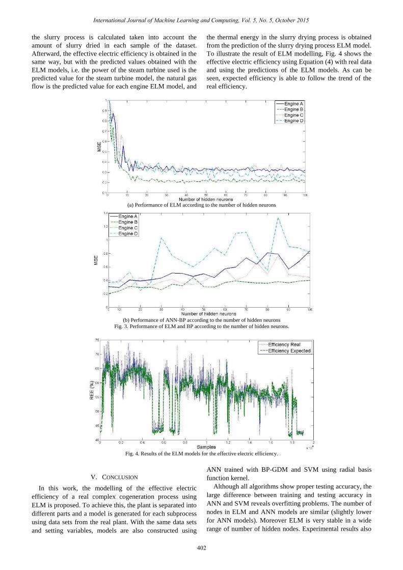
the slurry process is calculated taken into account the

amount of slurry dried in each sample of the dataset.

Afterward, the effective electric efficiency is obtained in the

same way, but with the predicted values obtained with the

ELM models, i.e. the power of the steam turbine used is the

predicted value for the steam turbine model, the natural gas

flow is the predicted value for each engine ELM model, and

the thermal energy in the slurry drying process is obtained

from the prediction of the slurry drying process ELM model.

To illustrate the result of ELM modelling, Fig. 4 shows the

effective electric efficiency using Equation (4) with real data

and using the predictions of the ELM models. As can be

seen, expected efficiency is able to follow the trend of the

real efficiency.

(a) Performance of ELM according to the number of hidden neurons

(b) Performance of ANN-BP according to the number of hidden neurons

Fig. 3. Performance of ELM and BP according to the number of hidden neurons.

Fig. 4. Results of the ELM models for the effective electric efficiency.

V. CONCLUSION

In this work, the modelling of the effective electric

efficiency of a real complex cogeneration process using

ELM is proposed. To achieve this, the plant is separated into

different parts and a model is generated for each subprocess

using data sets from the real plant. With the same data sets

and setting variables, models are also constructed using

ANN trained with BP-GDM and SVM using radial basis

function kernel.

Although all algorithms show proper testing accuracy, the

large difference between training and testing accuracy in

ANN and SVM reveals overfitting problems. The number of

nodes in ELM and ANN models are similar (slightly lower

for ANN models). Moreover ELM is very stable in a wide

range of number of hidden nodes. Experimental results also

International Journal of Machine Learning and Computing, Vol. 5, No. 5, October 2015

402

show that ELM is largely the fastest of all, spending

hundreds of times less than SVM and ANN.

As a conclusion of the experimental results, ELM

provides a robust learning algorithm, free of local minima,

without overfitting problems. ELM algorithm is very fast

learning and less dependent on human intervention than the

ANN-BP or SVM. All this characteristics make ELM

suitable for autonomous real-time monitoring of the plant.

REFERENCES

[1] Y. Li, B. Yang, Z. Wang, and X. Wang, “Fault pattern classification

of turbine-generator set based on artificial neural network,” in Proc. the International Conference on Computer Application and System

Modeling, 2010, vol. 15.

[2] H. Nikpey, M. Assadi, and P. Breuhaus, “Development of an artificialneural network model for combined heat and power micro

gas turbines,” in Proc. International Symposium on Innovations in

Intelligent Systems and Applications, 2012, pp. 1-5. [3] C. Cortes and V. Vapnik, “Support-vector networks,” Machine

Learning, vol. 20, no. 3, pp. 273-297, September 1995.

[4] G.-B. Huang, D. Wang, and Y. Lan, “Extreme learning machines: A survey,” International Journal of Machine Learning and Cybernetics,

vol. 2, no. 2, pp. 107-122, 2011. [5] G.-B. Huang, H. Zhou, X. Ding, and R. Zhang, “Extreme learning

machine for regression and multiclass classification,” IEEE

Transactions on Systems, Man, and Cybernetics, Part B: Cybernetics, vol. 42, no. 2, pp. 513-529, 2012.

[6] G.-B. Huang, Q.-Y. Zhu, and C.-K. Siew, “Extreme learning

machine: Theory and applications,” Neurocomputing, vol. 70, no. 1-3, pp. 489-501, 2006.

[7] J. E. R. Finker, I. del Campo, and V. Martínez, “An intelligent

embedded system for real-time adaptive extreme learning machine,” in Proc. 2014 IEEE Symposium on Intelligent Embedded Systems

2014, pp. 61-69.

[8] G.-B. Huang and L. Chen, “Convex incremental extreme learning machine,” Neurocomputing, vol. 70, no. 16-17, pp. 3056-3062, 2007.

[9] D. Serre, Matrices: Theory and Applications, Springer, 2001, ch. 8,

pp. 145-147.

[10] D. Mattera and S. Haykin, “Advances in kernel methods,” in Support

Vector Machines for Dynamic Reconstruction of a Chaotic System, B.

Schölkopf, C. J. C. Burges, and A. J. Smola, Eds. Cambridge, MA, USA: MIT Press, 1999, pp. 211-241.

[11] C.-C. Chang and C.-J. Lin, “LIBSVM: A library for support vector

machines,” ACM Transactions on Intelligent Systems and Technology, vol. 2, no. 3, 2011.

Sandra Seijo was born in Leon, Spain, in 1987. She

received the Dipl. Ing. degree in industrial chemistry,

and the M.Sc. degree from the University of Valladolid (UVA), in 2010 and 2012, respectively. She is a

predoctoral researcher (granted by the Basque

Government, Spain) from 2012. She is with the Department of Electricity and Electronics in the

University of the Basque Country (UPV/EHU), Bilbao,

Spain. Her research interests focus on 1) computational intelligence: artificial neural networks, fuzzy systems, and neuro-fuzzy systems; 2) Data

Mining and modelling of complex industrial processes; 3) Optimization of

complex industrial processes for maximum energy efficiency.

Inés del Campo was born in Buenos Aires, Argentina,

in 1961. She received the Licenciado degree in physics with specialization in electronics and automatics in

1987 and the Ph.D. degree in physics in 1993, both

from the University of the Basque Country (UPV/EHU), Bilbao, Spain. Currently she is a senior

lecturer in the Electricity and Electronics Department

of the Faculty of Sciences and Technology of the UPV/EHU. She has published articles in international journals and

conferences in the areas of electronics, computational intelligence,

intelligent control, ambient intelligence, and pattern recognition, among others. Her research interests mainly concern system-on-chip (SOC) design,

hardware/software codesign, reconfigurable hardware, pervasive

computing, artificial neural networks (ANNs), fuzzy systems, and genetic algorithms. She is also interested in the internet of things and its application

in the context of ubiquitous computing and ambient intelligence.

Javier Echanobe received the licenciado degree in

physics from the University of the Basque Country (UPV/EHU), Spain, and the Ph.D. degree from the

University of Navarra, Pamplona, Spain, in 1990 and

1998, respectively. He was a predoctoral researcher (granted by the Basque Government) from 1992 to

1996. He has been an associate professor in the

Department of Electricity and Electronics, UPV/EHU, from 1999 to 2009. Since 2009 he is a Senior Lecturer in that department.

His research interests focus on 1) digital electronics: embedded systems,

reconfigurable FPGAs, DSPs, SoPC; 2) computational intelligence: artificial neural networks, fuzzy systems, and neuro-fuzzy systems; 3)

ubiquitous computing: ambient intelligence, intelligent environments. Dr.

Echanobe has published many papers in international journals and conferences in most of those areas.

Javier García-Sedano received the licenciado degree

in physics, specialised in electronics and automation, from the University of the Basque Country

(UPV/EHU), Spain. The areas of his work and expertise

are in knowledge-based applications in manufacturing; hybrid symbolic-genetic learning techniques for

industrial process optimisation; intelligent agents for

industrial applications; semantic-based product management and configuration. With more than 26 years of experience in

these fields, he is the CEO and Founder of the OPTIMITIVE Group, with a

large track of successful innovative Artificial Intelligence applications in Industry. He worked previously in companies like IBERDROLA

Engineering, ORMAZABAL Group and TECNALIA Research

Corporation, having carried out RTD and Innovation Management responsibilities, achieving successful technology transfer to the industry in

the mentioned fields of specialisation.

International Journal of Machine Learning and Computing, Vol. 5, No. 5, October 2015

403