Embed Size (px)
Citation preview
Dynamics and Control-Oriented
Modelling of a Cogeneration System
Producing Compressed Air and Steam
Matthew J. Blom
Submitted in total fulfillment of the requirements
of the degree of Doctor of Philosophy
November, 2016
Department of Mechanical Engineering
The University of Melbourne
Victoria, Australia

ii
Abstract
Steam and compressed air are amongst the most significant consumers of industrial energy. Steam
with its excellent energy transport capabilities, is extensively used in power generation and indus-
trial applications while compressed air is frequently considered a ’fourth’ utility after electricity,
gas, and water. While steam is traditionally produced by fired boilers and compressed air by
electrically driven compressors, the desire for improved energy efficiency and reduced emissions
makes cogeneration of these, in particular with a gas turbine based device, an attractive alterna-
tive. Further improvements in performance, of both the individual systems and in a cogeneration
configuration, can be achieved through the use of model based control. However, these methods
first require an adequately accurate and yet computationally practical model of the system.
A gas turbine based air compressor concept and corresponding modeling has already been pre-
viously established and validated. Hence, this thesis therefore presents the development, validation
and model reduction of a physics based dynamic modelling approach for a boiler. The developed
modelling approach first extends an existing modelling framework for the previously stated gas
turbine system to cover non-ideal, single phase and non-ideal, two phase fluid systems with heat
transfer. This framework incorporates the behaviour of the main boiler components in determining
the source terms of the governing, one-dimensional conservation equations. The developed model
is then validated against measured data from the boiler of a large scale subcritical power plant
with multiple sub-systems, and informal model reduction is demonstrated using simple, physical
arguments.
This modelling approach is then combined with the existing gas turbine framework in a co-
generation application at smaller scale. In preparation for this the steady state, thermodynamic
analysis of several potential, small scale cogeneration plants producing compressed air and steam
are first considered. Formal model reduction by time scale separation and singular perturbation
theory is then examined for one of these small scale cogeneration plants, considering both the boiler
component time scales together with those from the previously established gas turbine model.
The model reductions of both the large scale and small scale power plants are both shown to be
acceptably accurate and run in faster than real time on a modern desktop PC. This demonstrates
that reduced order models potentially suitable for control applications can be developed from the
equations of fluid motion that observe the fundamental physics of boiler systems.
iii

iv ABSTRACT
Declaration
This is to certify that
(i) the thesis comprises only my original work towards the degree of Doctor of Philosophy,
(ii) due acknowledgment has been made in the text to all other material used,
(iii) the thesis is fewer than 100,000 words in length, exclusive of tables, maps, bibliographies and
appendices.
Signed,
Matthew Blom, November 2016
v

vi DECLARATION
Acknowledgments
I would like to thank the many people whose support and assistance contributed either directly or
indirectly to the completion of this thesis.
First and foremost I would like to thank my supervisors, Professors Michael Brear and Chris
Manzie, for their ongoing support, guidance, and patience over the course of my PhD.
Special thanks are extended to Andrew Gibbs of Ecogen Energy who provided the operational
data of the Newport Power Plant.
I would also like to thank my current and former colleagues from the thermodynamics group,
of whom there are far too many to name, for not only their friendship and company but also for
the many things I learned from them and their experiences. Of these people I would in particular
like to thank Ashley Wiese who provided the gas turbine model used in this thesis and from whom
I learned a great deal while working on the GTAC with him.
Lastly, but by no means least, I would like to thank my family, and in particular my parents,
for their ongoing support over the course of this PhD.
vii

viii ACKNOWLEDGMENTS
Contents
Abstract iii
Declaration v
Acknowledgments vii
Contents ix
List of Figures xiii
List of Tables xvii
Nomenclature xix
1 Introduction 1
1.1 Motivation . . . . . . . . . . . . . . . . . . . . . . . . . . . . . . . . . . . . . . . . 1
1.2 Compressed Air Production . . . . . . . . . . . . . . . . . . . . . . . . . . . . . . . 2
1.2.1 Conventional Compressed Air Production . . . . . . . . . . . . . . . . . . . 2
1.2.2 Gas Turbine Air Compressor (GTAC) . . . . . . . . . . . . . . . . . . . . . 3
1.3 Steam Generation . . . . . . . . . . . . . . . . . . . . . . . . . . . . . . . . . . . . 5
1.4 Thesis Outline . . . . . . . . . . . . . . . . . . . . . . . . . . . . . . . . . . . . . . 7
2 Literature Review 9
2.1 Introduction . . . . . . . . . . . . . . . . . . . . . . . . . . . . . . . . . . . . . . . . 9
2.2 Cogeneration Systems . . . . . . . . . . . . . . . . . . . . . . . . . . . . . . . . . . 9
2.2.1 Combined Cycle Gas Turbine . . . . . . . . . . . . . . . . . . . . . . . . . . 10
2.2.2 Combined Heat and Power . . . . . . . . . . . . . . . . . . . . . . . . . . . 12
2.2.3 Advanced Gas Turbine Cycles . . . . . . . . . . . . . . . . . . . . . . . . . . 12
2.2.4 Further Industrial Applications . . . . . . . . . . . . . . . . . . . . . . . . . 14
2.3 Control of Cogeneration Systems . . . . . . . . . . . . . . . . . . . . . . . . . . . . 15
2.3.1 Industry Standard Control . . . . . . . . . . . . . . . . . . . . . . . . . . . 16
2.3.1.1 Industry Standard Gas Turbine Control . . . . . . . . . . . . . . . 16
2.3.1.2 Industry Standard Thermal Plant Control . . . . . . . . . . . . . 19
2.3.2 Model Predictive Control . . . . . . . . . . . . . . . . . . . . . . . . . . . . 21
2.3.2.1 MPC Gas Turbine Control . . . . . . . . . . . . . . . . . . . . . . 22
2.3.2.2 MPC Boiler and Thermal Plant Control . . . . . . . . . . . . . . . 24
2.4 Transient Modelling of Cogeneration Systems . . . . . . . . . . . . . . . . . . . . . 25
ix
x CONTENTS
2.4.1 Gas Turbine Modelling . . . . . . . . . . . . . . . . . . . . . . . . . . . . . . 26
2.4.1.1 Phenomenological Models . . . . . . . . . . . . . . . . . . . . . . . 26
2.4.1.2 Gas Turbine Physics-Based Models . . . . . . . . . . . . . . . . . 27
2.4.1.2.1 Intercomponent Volume Models . . . . . . . . . . . . . . 27
2.4.1.2.2 Direct Numerical Simulation Models . . . . . . . . . . . . 28
2.4.2 Boiler Modelling . . . . . . . . . . . . . . . . . . . . . . . . . . . . . . . . . 30
2.4.2.1 Boiler Phenomenological Models . . . . . . . . . . . . . . . . . . . 30
2.4.2.2 Boiler Physics-Based Models . . . . . . . . . . . . . . . . . . . . . 31
2.5 Conclusion . . . . . . . . . . . . . . . . . . . . . . . . . . . . . . . . . . . . . . . . 34
2.6 Research Aims . . . . . . . . . . . . . . . . . . . . . . . . . . . . . . . . . . . . . . 34
3 Development of a Dynamic Model of a Boiler 37
3.1 Introduction . . . . . . . . . . . . . . . . . . . . . . . . . . . . . . . . . . . . . . . . 37
3.1.1 Model Structure . . . . . . . . . . . . . . . . . . . . . . . . . . . . . . . . . 38
3.1.2 Modelling Framework . . . . . . . . . . . . . . . . . . . . . . . . . . . . . . 40
3.2 Single-Phase Fluid Model . . . . . . . . . . . . . . . . . . . . . . . . . . . . . . . . 41
3.2.1 Single-Phase Forcing Term Map Derivation . . . . . . . . . . . . . . . . . . 44
3.2.1.1 Adiabatic Pipe of Uniform Cross-Sectional Area . . . . . . . . . . 44
3.2.1.2 Component of Uniform Cross-Sectional Area With Heat Transfer . 44
3.2.1.3 Component of Uniform Cross-Sectional Area With Heat Transfer
and Pressure Loss . . . . . . . . . . . . . . . . . . . . . . . . . . . 45
3.2.1.4 Adiabatic Components With Spatial Cross-Sectional Area Change 46
3.2.2 Furnace Model . . . . . . . . . . . . . . . . . . . . . . . . . . . . . . . . . . 47
3.2.3 Desuperheater . . . . . . . . . . . . . . . . . . . . . . . . . . . . . . . . . . 49
3.2.4 Circulation Pump . . . . . . . . . . . . . . . . . . . . . . . . . . . . . . . . 50
3.3 Two-Phase Fluid Model . . . . . . . . . . . . . . . . . . . . . . . . . . . . . . . . . 50
3.3.1 Two-Phase Forcing Term Map Derivation . . . . . . . . . . . . . . . . . . . 53
3.3.1.1 Adiabatic Pipe of Uniform Cross-Sectional Area . . . . . . . . . . 53
3.3.1.2 Component of Uniform Cross Sectional Area With Heat Transfer . 54
3.3.1.3 Adiabatic Component With Spatial Cross-Sectional Area Change 54
3.3.2 Phase Change Model . . . . . . . . . . . . . . . . . . . . . . . . . . . . . . . 55
3.4 Heat Transfer . . . . . . . . . . . . . . . . . . . . . . . . . . . . . . . . . . . . . . . 56
3.5 Boundary Condition Model . . . . . . . . . . . . . . . . . . . . . . . . . . . . . . . 57
3.6 Steam Drum Model . . . . . . . . . . . . . . . . . . . . . . . . . . . . . . . . . . . 59
3.7 Wall Model . . . . . . . . . . . . . . . . . . . . . . . . . . . . . . . . . . . . . . . . 62
3.8 Feedwater Models . . . . . . . . . . . . . . . . . . . . . . . . . . . . . . . . . . . . 65
3.8.1 Feedpump Model . . . . . . . . . . . . . . . . . . . . . . . . . . . . . . . . . 65
3.8.2 Flow Split . . . . . . . . . . . . . . . . . . . . . . . . . . . . . . . . . . . . . 65
3.9 Model Demonstration . . . . . . . . . . . . . . . . . . . . . . . . . . . . . . . . . . 66
3.9.1 Acoustic Behaviour of Adiabatic Pipe with Superheated Steam . . . . . . . 66
3.9.2 Acoustic Validation of Single-Phase, Constant-Area, Heat Transfer . . . . 67
3.9.3 Heat Exchangers . . . . . . . . . . . . . . . . . . . . . . . . . . . . . . . . . 70
3.9.4 Constant Temperature Fluid Heat Exchanger . . . . . . . . . . . . . . . . . 71
3.10 Conclusion . . . . . . . . . . . . . . . . . . . . . . . . . . . . . . . . . . . . . . . . 78
CONTENTS xi
4 Validation of the Boiler Model 81
4.1 Introduction . . . . . . . . . . . . . . . . . . . . . . . . . . . . . . . . . . . . . . . . 81
4.2 Modelling of the Newport Power Plant Boiler . . . . . . . . . . . . . . . . . . . . . 81
4.2.1 Newport Power Plant . . . . . . . . . . . . . . . . . . . . . . . . . . . . . . 81
4.2.2 Newport Boiler Model . . . . . . . . . . . . . . . . . . . . . . . . . . . . . . 83
4.3 Fitting Model Parameters . . . . . . . . . . . . . . . . . . . . . . . . . . . . . . . . 89
4.3.1 Steady State Model Calculation . . . . . . . . . . . . . . . . . . . . . . . . . 90
4.3.2 Air Preheating . . . . . . . . . . . . . . . . . . . . . . . . . . . . . . . . . . 91
4.3.3 Heat Transfer Coefficients . . . . . . . . . . . . . . . . . . . . . . . . . . . . 92
4.3.4 Pressure Drop Relations . . . . . . . . . . . . . . . . . . . . . . . . . . . . . 93
4.3.5 Steady State Results . . . . . . . . . . . . . . . . . . . . . . . . . . . . . . . 94
4.4 Dynamic Analysis . . . . . . . . . . . . . . . . . . . . . . . . . . . . . . . . . . . . 95
4.4.1 Effect of Thermal and Convective Time Scales . . . . . . . . . . . . . . . . 99
4.5 Model Reduction . . . . . . . . . . . . . . . . . . . . . . . . . . . . . . . . . . . . . 104
4.5.1 Structure Simplification . . . . . . . . . . . . . . . . . . . . . . . . . . . . . 104
4.5.2 Model Order Reduction . . . . . . . . . . . . . . . . . . . . . . . . . . . . . 105
4.5.3 Other Simplifications . . . . . . . . . . . . . . . . . . . . . . . . . . . . . . . 112
4.6 Conclusion . . . . . . . . . . . . . . . . . . . . . . . . . . . . . . . . . . . . . . . . 115
5 Cycle Analysis 119
5.1 Introduction . . . . . . . . . . . . . . . . . . . . . . . . . . . . . . . . . . . . . . . . 119
5.1.1 Cycle Performance Measures . . . . . . . . . . . . . . . . . . . . . . . . . . 119
5.1.2 Proposed Cycles . . . . . . . . . . . . . . . . . . . . . . . . . . . . . . . . . 120
5.2 Thermodynamic Model . . . . . . . . . . . . . . . . . . . . . . . . . . . . . . . . . 122
5.2.1 Compressor and Turbine . . . . . . . . . . . . . . . . . . . . . . . . . . . . . 123
5.2.2 Steam Injection . . . . . . . . . . . . . . . . . . . . . . . . . . . . . . . . . . 125
5.2.3 Combustion Chamber . . . . . . . . . . . . . . . . . . . . . . . . . . . . . . 125
5.2.4 Recuperator and HRSG . . . . . . . . . . . . . . . . . . . . . . . . . . . . . 126
5.2.5 Cycle Closure . . . . . . . . . . . . . . . . . . . . . . . . . . . . . . . . . . . 129
5.2.6 First Law Balance . . . . . . . . . . . . . . . . . . . . . . . . . . . . . . . . 129
5.3 Cycle Analysis Results . . . . . . . . . . . . . . . . . . . . . . . . . . . . . . . . . . 130
5.3.1 Steam Injection . . . . . . . . . . . . . . . . . . . . . . . . . . . . . . . . . . 130
5.3.2 Recuperation . . . . . . . . . . . . . . . . . . . . . . . . . . . . . . . . . . . 133
5.4 Greenhouse Gas Emissions Analysis . . . . . . . . . . . . . . . . . . . . . . . . . . 133
5.4.1 Emissions Model . . . . . . . . . . . . . . . . . . . . . . . . . . . . . . . . . 133
5.4.2 Emissions Results . . . . . . . . . . . . . . . . . . . . . . . . . . . . . . . . 136
5.5 Conclusion . . . . . . . . . . . . . . . . . . . . . . . . . . . . . . . . . . . . . . . . 137
6 Model Reduction of a Cogeneraton System 139
6.1 Introduction . . . . . . . . . . . . . . . . . . . . . . . . . . . . . . . . . . . . . . . . 139
6.2 Cogeneration System and Model . . . . . . . . . . . . . . . . . . . . . . . . . . . . 139
6.3 Model Reduction . . . . . . . . . . . . . . . . . . . . . . . . . . . . . . . . . . . . . 145
6.3.1 Single-Phase Model Non-Dimensionalisation . . . . . . . . . . . . . . . . . . 146
6.3.2 Wall Model . . . . . . . . . . . . . . . . . . . . . . . . . . . . . . . . . . . . 148
xii CONTENTS
6.3.3 Cogeneration System Model Reduction . . . . . . . . . . . . . . . . . . . . . 148
6.3.3.1 Time Scale Comparison . . . . . . . . . . . . . . . . . . . . . . . . 148
6.3.4 Model Reduction Analysis . . . . . . . . . . . . . . . . . . . . . . . . . . . . 152
6.4 Conclusion . . . . . . . . . . . . . . . . . . . . . . . . . . . . . . . . . . . . . . . . 163
7 Conclusions and Future Work 165
7.1 Conclusions . . . . . . . . . . . . . . . . . . . . . . . . . . . . . . . . . . . . . . . . 165
7.2 Future Work . . . . . . . . . . . . . . . . . . . . . . . . . . . . . . . . . . . . . . . 168
Bibliography 171
A Derivation of the Boiler Dynamic Model 185
A.1 Single Phase Model . . . . . . . . . . . . . . . . . . . . . . . . . . . . . . . . . . . . 185
A.1.1 General Single Phase Model Derivation . . . . . . . . . . . . . . . . . . . . 185
A.1.2 Single Phase Model Forcing Term Derivation . . . . . . . . . . . . . . . . . 189
A.1.2.1 Adiabatic and Uniform Cross-Sectional Area Pipe . . . . . . . . . 189
A.1.2.2 Uniform Cross-Sectional Area Heat Transfer . . . . . . . . . . . . 189
A.1.2.3 Uniform Cross-Sectional Area Heat Transfer With Defined Pressure
Loss . . . . . . . . . . . . . . . . . . . . . . . . . . . . . . . . . . . 190
A.1.2.4 Adiabatic Spatial Cross-Sectional Area Change . . . . . . . . . . . 191
A.1.3 Furnace Model . . . . . . . . . . . . . . . . . . . . . . . . . . . . . . . . . . 192
A.1.4 Desuperheater Model . . . . . . . . . . . . . . . . . . . . . . . . . . . . . . 194
A.1.5 Circulation Pump . . . . . . . . . . . . . . . . . . . . . . . . . . . . . . . . 195
A.2 Two Phase Model . . . . . . . . . . . . . . . . . . . . . . . . . . . . . . . . . . . . 196
A.2.1 General Two Phase Model Derivation . . . . . . . . . . . . . . . . . . . . . 196
A.2.2 Two Phase Model Forcing Term Derivation . . . . . . . . . . . . . . . . . . 214
A.2.2.1 Adiabatic and Uniform Cross-Sectional Area Pipe . . . . . . . . . 214
A.2.2.2 Uniform Cross-Sectional Area Heat Transfer . . . . . . . . . . . . 215
A.2.2.3 Adiabatic Spatial Cross-Sectional Area Change . . . . . . . . . . . 216
A.2.3 Phase Change Model . . . . . . . . . . . . . . . . . . . . . . . . . . . . . . . 217
A.3 Steam Drum . . . . . . . . . . . . . . . . . . . . . . . . . . . . . . . . . . . . . . . 219
A.4 Feedwater Model . . . . . . . . . . . . . . . . . . . . . . . . . . . . . . . . . . . . . 226
A.4.1 Feedpump Model . . . . . . . . . . . . . . . . . . . . . . . . . . . . . . . . . 226
A.4.2 Flow Split Model . . . . . . . . . . . . . . . . . . . . . . . . . . . . . . . . . 226
A.5 Wall Model . . . . . . . . . . . . . . . . . . . . . . . . . . . . . . . . . . . . . . . . 227
B Newport Boiler Steady State Calculation 231
C Non-Dimensionalisation of the Single Phase Model 235
List of Figures
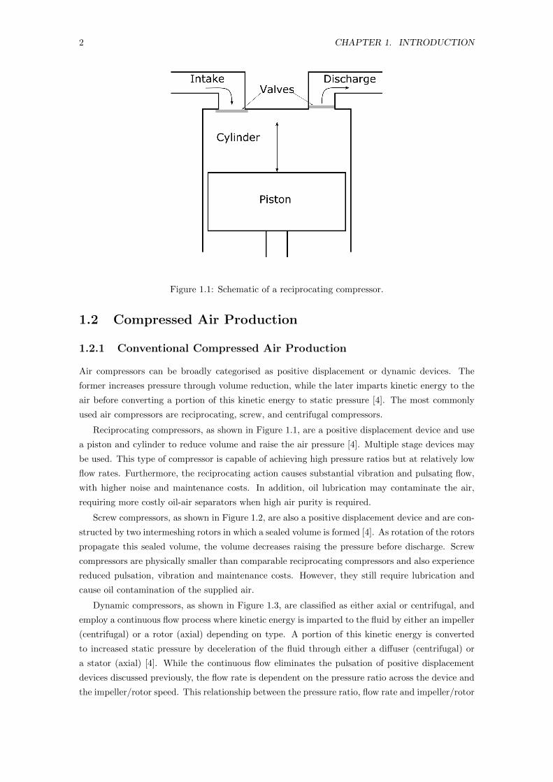
1.1 Schematic of a reciprocating compressor. . . . . . . . . . . . . . . . . . . . . . . . . 2
1.2 Schematic of a screw compressor. . . . . . . . . . . . . . . . . . . . . . . . . . . . . 3
1.3 Diagram of axial and centrifugal compressors. . . . . . . . . . . . . . . . . . . . . . 4
1.4 The GTAC concept with optional intercooler and recuperator (reproduced from [1]). 4
1.5 Basic fire tube boiler. . . . . . . . . . . . . . . . . . . . . . . . . . . . . . . . . . . 5
1.6 Basic water tube boiler. . . . . . . . . . . . . . . . . . . . . . . . . . . . . . . . . . 5
1.7 General schematic of a drum boiler. . . . . . . . . . . . . . . . . . . . . . . . . . . 6
2.1 Schematic of a combined cycle gas turbine. . . . . . . . . . . . . . . . . . . . . . . 11
2.2 Schematic of a Steam Injected Gas Turbine (STIG) cycle. . . . . . . . . . . . . . . 13
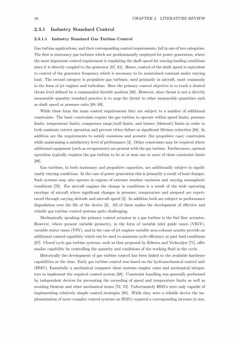
2.3 Example of standard fuel control structure for a turbofan engine [2]. . . . . . . . . 18
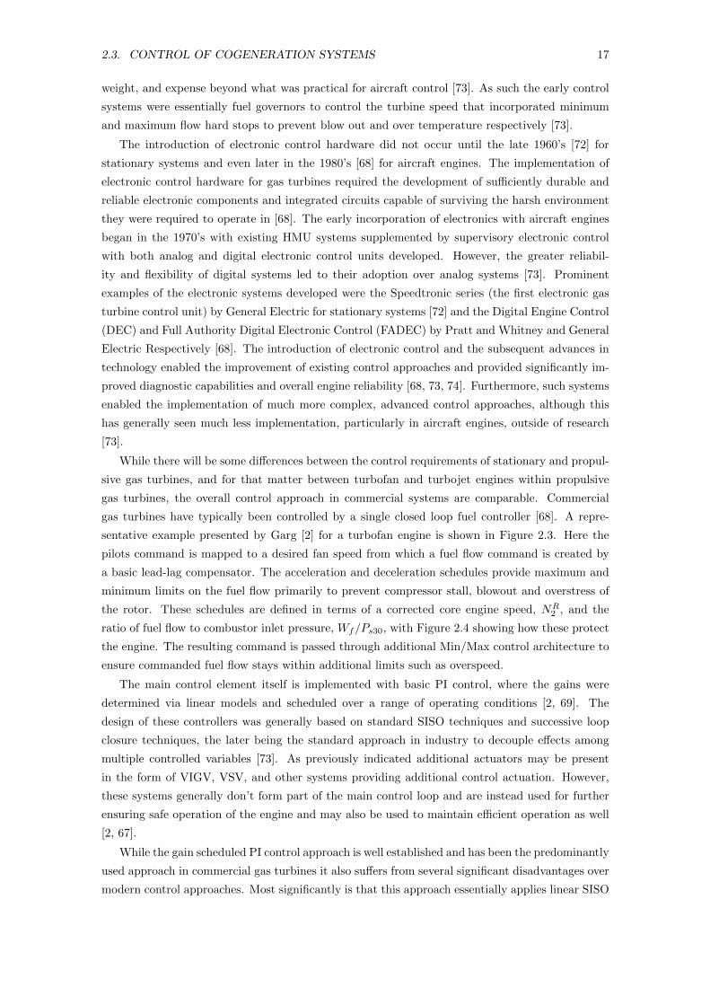
2.4 Representative diagram of acceleration and deceleration schedules intended to pro-
tect engine [2]. . . . . . . . . . . . . . . . . . . . . . . . . . . . . . . . . . . . . . . 18
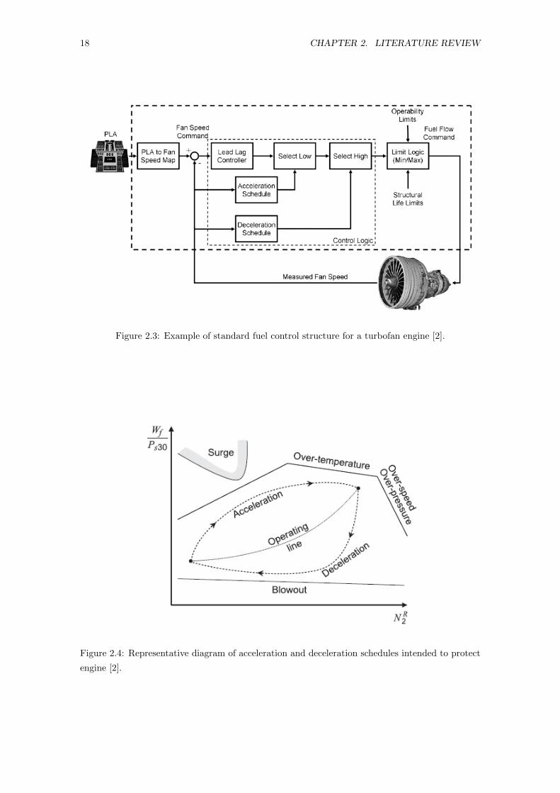
2.5 Basic Schematic of a drum type boiler . . . . . . . . . . . . . . . . . . . . . . . . . 20
3.1 Typical layout of a boiler . . . . . . . . . . . . . . . . . . . . . . . . . . . . . . . . 38
3.2 General model structure for the steam path . . . . . . . . . . . . . . . . . . . . . . 39
3.3 Schematic of a general single-phase element with heat transfer . . . . . . . . . . . . 43
3.4 Schematic of the furnace element . . . . . . . . . . . . . . . . . . . . . . . . . . . . 47
3.5 Schematic of a desuperheater element . . . . . . . . . . . . . . . . . . . . . . . . . 49
3.6 Schematic of a general two-phase element with heat transfer . . . . . . . . . . . . . 53
3.7 Schematics of both upstream and downstream boundary condition elements for
LODI conditions . . . . . . . . . . . . . . . . . . . . . . . . . . . . . . . . . . . . . 58
3.8 Schematic of the steam drum . . . . . . . . . . . . . . . . . . . . . . . . . . . . . . 59
3.9 Schematic of the drum liquid inlet . . . . . . . . . . . . . . . . . . . . . . . . . . . 60
3.10 Schematic of the drum two-phase inlet noting that solid lines denote inputs while
dashed lines denote states. . . . . . . . . . . . . . . . . . . . . . . . . . . . . . . . . 61
3.11 Schematic of a wall element showing nominal heat transfer paths. . . . . . . . . . . 63
3.12 Schematic representation of heat transfer surface for the case of a tube with internal
heat transfer. . . . . . . . . . . . . . . . . . . . . . . . . . . . . . . . . . . . . . . . 64
3.13 Schematic of a feedpump element . . . . . . . . . . . . . . . . . . . . . . . . . . . . 65
3.14 Schematic of a flow split element . . . . . . . . . . . . . . . . . . . . . . . . . . . . 66
3.15 The speed of sound in steam for increasing degrees of superheat for simulation and
from REFPROP . . . . . . . . . . . . . . . . . . . . . . . . . . . . . . . . . . . . . 67
xiii
xiv LIST OF FIGURES
3.16 Comparison of reflection and transmission coefficients with nitrogen as the work-
ing fluid for the case of heat addition showing simulated reflection coefficients (◦),simulated transmission coefficients (×), analytic reflection coefficients ( ), and
analytic transmission coefficients ( ). . . . . . . . . . . . . . . . . . . . . . . . . . 69
3.17 Comparison of reflection and transmission coefficients with high temperature steam
as the working fluid for the case of heat addition showing simulated reflection co-
efficients (◦), simulated transmission coefficients (×), analytic reflection coefficients
( ), and analytic transmission coefficients ( ). . . . . . . . . . . . . . . . . . . 70
3.18 Initial temperature profiles of the counterflow heat exchanger . . . . . . . . . . . . 72
3.19 Initial temperature profiles of the parallel-flow heat exchanger . . . . . . . . . . . . 73
3.20 Results of the counterflow configuration simulations . . . . . . . . . . . . . . . . . 74
3.21 Results of the parallel-flow configuration simulations . . . . . . . . . . . . . . . . . 75
3.22 Schematic of the heat exchanger set up for the constant temperature fluid heat
exchanger case. . . . . . . . . . . . . . . . . . . . . . . . . . . . . . . . . . . . . . . 76
3.23 Comparison of simulated ( ) and analytic ( ) solutions for a step change in the
constant temperature fluid . . . . . . . . . . . . . . . . . . . . . . . . . . . . . . . . 78
4.1 Schematic of the Newport power station boiler steam path showing available oper-
ating data . . . . . . . . . . . . . . . . . . . . . . . . . . . . . . . . . . . . . . . . . 82
4.2 The Newport power station gas path showing locations of steam path components 84
4.3 Schematic of the structure of the model of the Newport boiler . . . . . . . . . . . . 86
4.4 Data for the gas path economiser inlet temperature against the air flow rate. . . . 91
4.5 Fit of the heat transfer coefficients . . . . . . . . . . . . . . . . . . . . . . . . . . . 93
4.6 Percentage errors between model and data for the steam outlet . . . . . . . . . . . 96
4.7 Percentage errors between model and data for the economiser and desuperheater . 97
4.8 Simulation inputs for the fuel, air, reheater, feedwater, and spray water . . . . . . 98
4.9 Simulation inputs for the steam and gas path outlet pressures . . . . . . . . . . . . 99
4.10 Simulation results for the steam outlet . . . . . . . . . . . . . . . . . . . . . . . . . 100
4.11 Simulation results for the steam drum . . . . . . . . . . . . . . . . . . . . . . . . . 101
4.12 Simulation results for the desuperheater . . . . . . . . . . . . . . . . . . . . . . . . 102
4.13 Simulation results for the economiser and gas path . . . . . . . . . . . . . . . . . . 103
4.14 Component wall time constants and residence times . . . . . . . . . . . . . . . . . 104
4.15 Schematic of reduced model case 1. . . . . . . . . . . . . . . . . . . . . . . . . . . . 106
4.16 Schematic of reduced model case 2. . . . . . . . . . . . . . . . . . . . . . . . . . . . 107
4.17 Schematic of reduced model case 3. . . . . . . . . . . . . . . . . . . . . . . . . . . . 107
4.18 Simplified models simulation results for the steam outlet . . . . . . . . . . . . . . . 108
4.19 Simplified models simulation results for the steam drum . . . . . . . . . . . . . . . 109
4.20 Reduced order models simulation results for the steam outlet . . . . . . . . . . . . 110
4.21 Reduced order models simulation results for the steam drum . . . . . . . . . . . . 111
4.22 Gas constant compressibilities for air and combustion products . . . . . . . . . . . 114
4.23 Further simplified reduced order models simulation results for the steam outlet . . 116
4.24 Further simplified reduced order models simulation results for the steam drum . . 117
5.1 Schematics of advanced GTAC cycles . . . . . . . . . . . . . . . . . . . . . . . . . . 121
LIST OF FIGURES xv
5.2 Block diagram of the STIGTAC model . . . . . . . . . . . . . . . . . . . . . . . . . 124
5.3 Schematic of a general heat exchanger set up as used for the recuperator . . . . . . 127
5.4 Schematic of the HRSG . . . . . . . . . . . . . . . . . . . . . . . . . . . . . . . . . 128
5.5 Compressed air efficiency results for STIGTAC and recuperated cycles . . . . . . . 131
5.6 Overall efficiency for GTAC and STIGTAC cycles . . . . . . . . . . . . . . . . . . . 132
5.7 Compressed air efficiency for recuperated STIGTAC . . . . . . . . . . . . . . . . . 134
5.8 Overall efficiency for recuperated STIGTAC . . . . . . . . . . . . . . . . . . . . . . 135
5.9 CO2 mitigation of natural gas fired STIGTAC . . . . . . . . . . . . . . . . . . . . . 137
6.1 Schematic of GTAC cogeneration model . . . . . . . . . . . . . . . . . . . . . . . . 141
6.2 Schematic of the simulation layout of the GTAC model (reproduced from [3]). . . . 142
6.3 Characteristic map of the feedpump. . . . . . . . . . . . . . . . . . . . . . . . . . . 144
6.4 Cogeneration model reduction cases simulation results for the bled air . . . . . . . 154
6.5 Cogeneration model reduction cases simulation results for the shaft speed and the
GTAC convergent section wall temperature . . . . . . . . . . . . . . . . . . . . . . 155
6.6 Cogeneration model reduction cases simulation results for the GTAC turbine and
exhaust wall temperatures . . . . . . . . . . . . . . . . . . . . . . . . . . . . . . . . 156
6.7 Cogeneration model reduction cases simulation results for the GTAC exhaust con-
ditions . . . . . . . . . . . . . . . . . . . . . . . . . . . . . . . . . . . . . . . . . . . 157
6.8 Cogeneration model reduction cases simulation results for the steam outlet . . . . 158
6.9 Cogeneration model reduction cases simulation results for the steam drum . . . . . 159
6.10 Cogeneration model reduction cases simulation results for the economiser and riser
wall temperatures . . . . . . . . . . . . . . . . . . . . . . . . . . . . . . . . . . . . . 160
6.11 Cogeneration model reduction cases simulation results for the superheater wall tem-
peratures . . . . . . . . . . . . . . . . . . . . . . . . . . . . . . . . . . . . . . . . . 161

xvi LIST OF FIGURES
List of Tables
2.1 Proportion of industrial electrical consumption used for compressed air production. 14
2.2 Steam consumption as a proportion of industrial energy consumption. . . . . . . . 15
3.1 Geometry and heat transfer coefficients for the heat exchanger simulation cases . . 71
3.2 Upstream inlet fluid conditions for the heat exchanger simulation cases . . . . . . . 71
4.1 Representative geometry for the economiser components. . . . . . . . . . . . . . . . 87
4.2 Representative geometry for the waterwall components. . . . . . . . . . . . . . . . 87
4.3 Representative geometry for the components of the superheater stages including the
desuperheater. . . . . . . . . . . . . . . . . . . . . . . . . . . . . . . . . . . . . . . 88
4.4 Representative geometry for the gas path components. . . . . . . . . . . . . . . . . 88
4.5 Representative geometry for the steam drum. . . . . . . . . . . . . . . . . . . . . . 89
4.6 Material properties for the metal volumes associated with each model component. 89
4.7 Heat transfer coefficient fitting parameters and resulting values over a range of
operating conditions. . . . . . . . . . . . . . . . . . . . . . . . . . . . . . . . . . . . 93
4.8 Fitted pressure drop parameters for the economiser and superheater. . . . . . . . . 94
4.9 Coefficients for the quadratic fits of the two-phase saturation properties. . . . . . . 112
4.10 Coefficients for the quadratic fits of the liquid phase properties . . . . . . . . . . . 113
4.11 Coefficients for the quadratic fits of the vapour phase properties . . . . . . . . . . 113
4.12 Coefficients for the quadratic fits of the enthalpy of air. . . . . . . . . . . . . . . . 114
4.13 Coefficients for the quadratic fits of the post-combustion gas enthalpy. . . . . . . . 115
5.1 Results of selected points for enthalpy balance over STIGTAC cycle. . . . . . . . . 130
6.1 Boiler model geometry for the main steam path components and the gas path along
with the associated convective heat transfer coefficients. . . . . . . . . . . . . . . . 143
6.2 Boiler model geometry for the steam drum. . . . . . . . . . . . . . . . . . . . . . . 143
6.3 Boiler model wall properties. . . . . . . . . . . . . . . . . . . . . . . . . . . . . . . 143
6.4 Non-dimensional terms for the single-phase model. . . . . . . . . . . . . . . . . . . 147
6.5 Representative time scales of both the GTAC and boiler dynamics . . . . . . . . . 149
6.6 Comparison of computation times considering different mapping options for each
reduction case. . . . . . . . . . . . . . . . . . . . . . . . . . . . . . . . . . . . . . . 162
xvii

xviii LIST OF TABLES
Nomenclature
General Variables
∆hfo Enthalpy of formation (J/kg)
m Fluid mass flow rate (kg/s)
Li Characteristic wave amplitude
a Cost function weighting terms (-), wave amplitude ratio terms (-)
Acr Flow path cross-sectional area (m2)
Asurf Wall surface area (m2)
b Wave amplitude ratio terms (-)
Bi Biot number (-)
C Pressure loss constant term, analytic heat exchanger model terms
c Mass fraction (-), speed of sound (m/s), heat capacity rate (W/K)
Cp Fluid specific heat at constant pressure (J/kgK)
cv,f GTAC fuel valve flow coefficient (US gallons/minute)
Cw Specific heat of wall element (J/kgK)
CMF Compressor corrected mass flow rate (kg/s)
D Analytic heat exchanger model parameters (-)
d Wave amplitude ratio terms (-)
Dh Hydraulic diameter (m)
E Energy term in LODI boundary conditions (J/kg)
e Specific internal energy (J)
fs Source term associated with body forces
fw Source term associated with friction
FAR Fuel-air ratio (-)
xix
xx NOMENCLATURE
H Enthalpy (W)
h Specific enthalpy (J/kg), convective heat transfer coefficient (W/m2K)
I Incident wave amplitude (-)
J Cost function (-), shaft rotational inertia (kgm2)
k Thermal conductivity (W/mK)
k1 Heat transfer coefficient fitting parameter
k2 Heat transfer coefficient fitting parameter
L Length (m)
LCV Lower calorific value (J/kg)
M Molar mass (g/mol), Mach number (-)
m Mass (kg)
mi Forcing term for row i
N Number of elements in a component, shaft speed (RPM)
Ni Analytic heat exchanger model parameters (-)
Npump Feedpump shaft speed (RPM)
NTU Number of Transfer Units (-)
Ps Static pressure (kPa)
Q Heat transfer or release rate (W)
R Specific gas constant (J/kgK), reflected wave amplitude (-)
rp Compressor/turbine pressure ratio (-)
rtip Radius of the compressor exducer tip (m)
S Entropy (W/K), steam ratio (-)
s Specific entropy (J/kgK)
SR Slip ratio (-)
T Transmitted wave amplitude (-)
t Time (s)
tr Residence time (s)
Ts Static temperature (K)
U Overall heat transfer coefficient (W/m2K)
NOMENCLATURE xxi
u Fluid velocity (m/s)
V Volume (m3)
w Wall perimeter with respect to flow direction (m), specific work (J/kg)
x Dryness Fraction (-)
y Spatial coordinate (m), mole fraction (-)
Matrix/Vector Variables
A Matrix of coefficients of temporal derivative terms
B Matrix of coefficients of spatial derivative terms
E Vector of fluid inertia terms
F Vector of source terms
G Matrix of influence coefficients
md Vector of measured disturbances
M Vector of mi terms
u Vector of model inputs
x Set of dynamic states
z GTAC model states
z′ Set of quasi-steady states
Greek Variables
α Void fraction (-), absorptivity (-)
αp Pressure loss fitted parameter
τ Reference torque (Nm)
β Pressure loss scaling factor
χCO2 Percentage CO2 emissions mitigation (%)
χi Coefficients of two phase differential conservation of momentum equation
ε Emissivity (-), fluid inertia term, heat exchanger effectiveness (-)
η Device efficiency (-)
γ Adiabatic index (-)
λ Characteristic velocity (m/s), analytic heat exchanger model parameters
ω Shaft rotational speed (rad/s)
xxii NOMENCLATURE
φ Equivalence ratio (-)
ρ Density (kg/m3
σ Stefan-Boltzmann constant (W/m2K4)
σslip Compressor impeller slip factor (-)
τ Time constant (s)
θbl GTAC bleed valve angular position (◦)
ξi Coefficients of two phase differential conservation of energy equation
ζ Perturbation parameter
Super/Subscripts
0 At length 0, initial condition
∞ Final condition
a Air
as Air-steam mixture
b Bleed
bi Boiler inlet
bo Boiler outlet
c Cold side, compressor
c Constant temperature fluid
ca Compressed air
cc Combustion chamber
ci Compressor inlet, cold side inlet
co Compressor outlet, cold side outlet
cogen Cogenerated steam
cond Conduction
conv Convection, GTAC convergent section
ds Desuperheater
eco Economiser
el Subelement of an element
ex Exhaust
NOMENCLATURE xxiii
ext external
f Fuel
g Gas, vapour
h Hot side
hi Hot side inlet
ho Hot side outlet
hrsg Heat recovery steam generator (boiler)
in Fluid element inlet
int Internal
l Liquid, left boundary, at length position l
leak Feedpump leak off
o Overall system
out Fluid element outlet
r Right boundary
rad Radiation
ref Reference, corrected value
s Steam, single phase fluid
sh superheater
si Steam injection
so Steam outlet
spray Spray water
stoich Stoichiometric ratio
t Stagnation quantity, turbine
ti Turbine inlet
to Turbine outlet
tp Two Phase
vap Vapourisation
w Wall, spray water
wi Water inlet

xxiv NOMENCLATURE
Chapter 1
Introduction
1.1 Motivation
Compressed air and steam are amongst the most significant consumers of energy in industry [4, 5].
The use of compressed air can be found across a wide variety of industries including apparel, food,
metal fabrication, textiles, mining and more [6]. These applications can include pneumatic tools
and actuation, drying, agitating fluids, spraying, and air starting of gas turbines amongst others
[4]. Compressed air is typically produced by electrically-driven air compressors [4]. This represents
a substantial burden on electricity distribution infrastructure which is of particular concern where
distribution networks are already under strain or limited in coverage. In nations where the use of
fossil fuels, and in particular coal, represent a significant proportion of electricity generation, the
production of compressed air also contributes to increased greenhouse gas emissions. Hence, there
is motivation for methods to reduce the burden compressed air production places on electrical
infrastructure.
Steam is used extensively in power generation and across a broad range of industries with
both heating and direct contact applications [7]. Industrial steam production is predominantly
achieved by gas-fired boilers. More recently, however, steam generation by cogeneration with
power generators has seen growing interest. In the US alone, steam generation is split almost
fifty-fifty between conventional boilers and cogeneration systems [8]. Considering the significant
industrial energy consumption in producing steam, there is considerable potential for reducing
overall energy consumption by the further adoption of cogeneration.
This thesis therefore examines the cogeneration of compressed air and steam. Particular at-
tention is given to the dynamic modelling required for the model-based control of such a system.
The following sections will examine the production of compressed air and steam in more detail,
including a novel air compressor concept proposed by Wiese et al [9]. The final section will provide
an outline of the thesis.
1
2 CHAPTER 1. INTRODUCTION
Figure 1.1: Schematic of a reciprocating compressor.
1.2 Compressed Air Production
1.2.1 Conventional Compressed Air Production
Air compressors can be broadly categorised as positive displacement or dynamic devices. The
former increases pressure through volume reduction, while the later imparts kinetic energy to the
air before converting a portion of this kinetic energy to static pressure [4]. The most commonly
used air compressors are reciprocating, screw, and centrifugal compressors.
Reciprocating compressors, as shown in Figure 1.1, are a positive displacement device and use
a piston and cylinder to reduce volume and raise the air pressure [4]. Multiple stage devices may
be used. This type of compressor is capable of achieving high pressure ratios but at relatively low
flow rates. Furthermore, the reciprocating action causes substantial vibration and pulsating flow,
with higher noise and maintenance costs. In addition, oil lubrication may contaminate the air,
requiring more costly oil-air separators when high air purity is required.
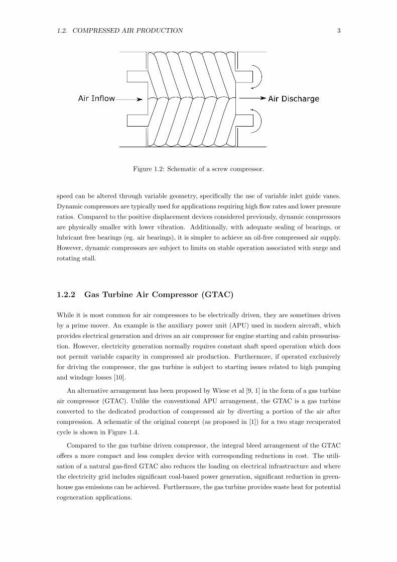
Screw compressors, as shown in Figure 1.2, are also a positive displacement device and are con-
structed by two intermeshing rotors in which a sealed volume is formed [4]. As rotation of the rotors
propagate this sealed volume, the volume decreases raising the pressure before discharge. Screw
compressors are physically smaller than comparable reciprocating compressors and also experience
reduced pulsation, vibration and maintenance costs. However, they still require lubrication and
cause oil contamination of the supplied air.
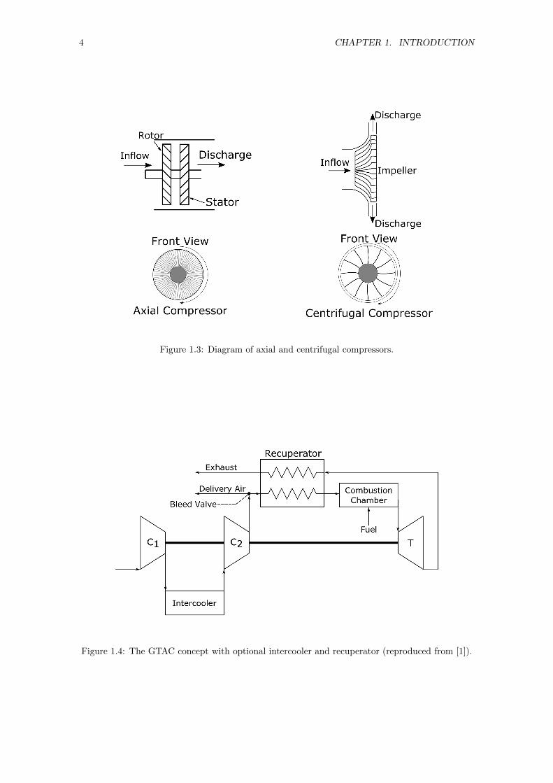
Dynamic compressors, as shown in Figure 1.3, are classified as either axial or centrifugal, and
employ a continuous flow process where kinetic energy is imparted to the fluid by either an impeller
(centrifugal) or a rotor (axial) depending on type. A portion of this kinetic energy is converted
to increased static pressure by deceleration of the fluid through either a diffuser (centrifugal) or
a stator (axial) [4]. While the continuous flow eliminates the pulsation of positive displacement
devices discussed previously, the flow rate is dependent on the pressure ratio across the device and
the impeller/rotor speed. This relationship between the pressure ratio, flow rate and impeller/rotor
1.2. COMPRESSED AIR PRODUCTION 3
Figure 1.2: Schematic of a screw compressor.
speed can be altered through variable geometry, specifically the use of variable inlet guide vanes.
Dynamic compressors are typically used for applications requiring high flow rates and lower pressure
ratios. Compared to the positive displacement devices considered previously, dynamic compressors
are physically smaller with lower vibration. Additionally, with adequate sealing of bearings, or
lubricant free bearings (eg. air bearings), it is simpler to achieve an oil-free compressed air supply.
However, dynamic compressors are subject to limits on stable operation associated with surge and
rotating stall.
1.2.2 Gas Turbine Air Compressor (GTAC)
While it is most common for air compressors to be electrically driven, they are sometimes driven
by a prime mover. An example is the auxiliary power unit (APU) used in modern aircraft, which
provides electrical generation and drives an air compressor for engine starting and cabin pressurisa-
tion. However, electricity generation normally requires constant shaft speed operation which does
not permit variable capacity in compressed air production. Furthermore, if operated exclusively
for driving the compressor, the gas turbine is subject to starting issues related to high pumping
and windage losses [10].
An alternative arrangement has been proposed by Wiese et al [9, 1] in the form of a gas turbine
air compressor (GTAC). Unlike the conventional APU arrangement, the GTAC is a gas turbine
converted to the dedicated production of compressed air by diverting a portion of the air after
compression. A schematic of the original concept (as proposed in [1]) for a two stage recuperated
cycle is shown in Figure 1.4.
Compared to the gas turbine driven compressor, the integral bleed arrangement of the GTAC
offers a more compact and less complex device with corresponding reductions in cost. The utili-
sation of a natural gas-fired GTAC also reduces the loading on electrical infrastructure and where
the electricity grid includes significant coal-based power generation, significant reduction in green-
house gas emissions can be achieved. Furthermore, the gas turbine provides waste heat for potential
cogeneration applications.
4 CHAPTER 1. INTRODUCTION
Figure 1.3: Diagram of axial and centrifugal compressors.
Figure 1.4: The GTAC concept with optional intercooler and recuperator (reproduced from [1]).
1.3. STEAM GENERATION 5
Figure 1.5: Basic fire tube boiler.
Figure 1.6: Basic water tube boiler.
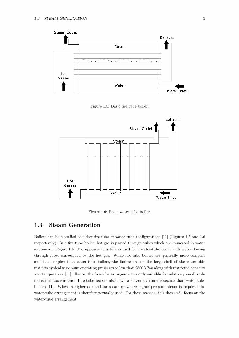
1.3 Steam Generation
Boilers can be classified as either fire-tube or water-tube configurations [11] (Figures 1.5 and 1.6
respectively). In a fire-tube boiler, hot gas is passed through tubes which are immersed in water
as shown in Figure 1.5. The opposite structure is used for a water-tube boiler with water flowing
through tubes surrounded by the hot gas. While fire-tube boilers are generally more compact
and less complex than water-tube boilers, the limitations on the large shell of the water side
restricts typical maximum operating pressures to less than 2500 kPag along with restricted capacity
and temperature [11]. Hence, the fire-tube arrangement is only suitable for relatively small scale
industrial applications. Fire-tube boilers also have a slower dynamic response than water-tube
boilers [11]. Where a higher demand for steam or where higher pressure steam is required the
water-tube arrangement is therefore normally used. For these reasons, this thesis will focus on the
water-tube arrangement.
6 CHAPTER 1. INTRODUCTION
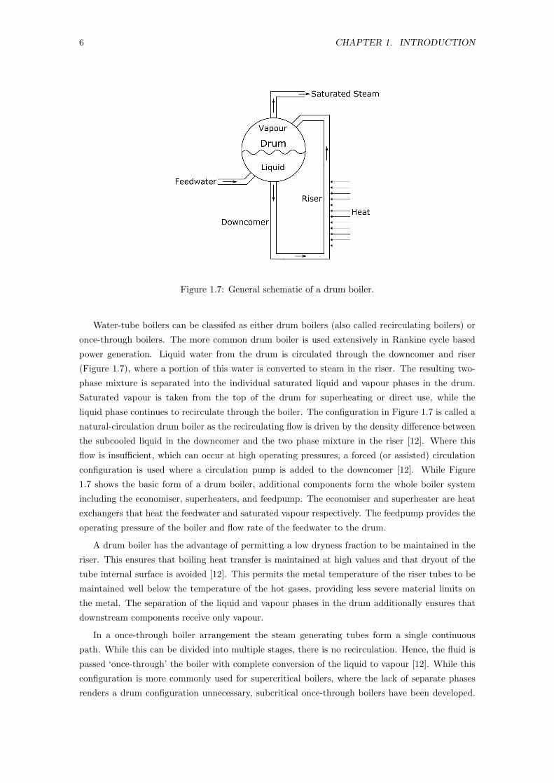
Figure 1.7: General schematic of a drum boiler.
Water-tube boilers can be classifed as either drum boilers (also called recirculating boilers) or
once-through boilers. The more common drum boiler is used extensively in Rankine cycle based
power generation. Liquid water from the drum is circulated through the downcomer and riser
(Figure 1.7), where a portion of this water is converted to steam in the riser. The resulting two-
phase mixture is separated into the individual saturated liquid and vapour phases in the drum.
Saturated vapour is taken from the top of the drum for superheating or direct use, while the
liquid phase continues to recirculate through the boiler. The configuration in Figure 1.7 is called a
natural-circulation drum boiler as the recirculating flow is driven by the density difference between
the subcooled liquid in the downcomer and the two phase mixture in the riser [12]. Where this
flow is insufficient, which can occur at high operating pressures, a forced (or assisted) circulation
configuration is used where a circulation pump is added to the downcomer [12]. While Figure
1.7 shows the basic form of a drum boiler, additional components form the whole boiler system
including the economiser, superheaters, and feedpump. The economiser and superheater are heat
exchangers that heat the feedwater and saturated vapour respectively. The feedpump provides the
operating pressure of the boiler and flow rate of the feedwater to the drum.
A drum boiler has the advantage of permitting a low dryness fraction to be maintained in the
riser. This ensures that boiling heat transfer is maintained at high values and that dryout of the
tube internal surface is avoided [12]. This permits the metal temperature of the riser tubes to be
maintained well below the temperature of the hot gases, providing less severe material limits on
the metal. The separation of the liquid and vapour phases in the drum additionally ensures that
downstream components receive only vapour.
In a once-through boiler arrangement the steam generating tubes form a single continuous
path. While this can be divided into multiple stages, there is no recirculation. Hence, the fluid is
passed ‘once-through’ the boiler with complete conversion of the liquid to vapour [12]. While this
configuration is more commonly used for supercritical boilers, where the lack of separate phases
renders a drum configuration unnecessary, subcritical once-through boilers have been developed.
1.4. THESIS OUTLINE 7
The main advantage of a once through boiler is a significantly faster dynamic response. However,
a subcritical once through boiler is subject to variable position of dryout in the steam generating
tubes [12]. This presents a more complicated design and control problem to ensure dryout occurs
within an acceptable region of the boiler.
While both fire tube and once-through boilers offer some advantages this thesis will focus on
the more commonly used conventional drum boiler configuration.
1.4 Thesis Outline
Chapter 2 initially presents an overview of cogeneration, with consideration given to the most
commonly implemented gas turbine based forms. This includes an identification of areas where
cogeneration shows merit but has not previously been considered, with particular attention given
to compressed air and steam production. Since cogeneration presents additional control consid-
erations, an examination of the current industry practice in gas turbine and steam plant control
is presented. This identifies a number of limitations in the control of cogeneration and individual
systems. Approaches for overcoming these limitations are examined with model based control
demonstrating promise. Since model based control requires a suitable model, the remainder of
Chapter 2 therefore examines various models of gas turbines and boilers, with emphasis given to
those suitable for control applications.
A transient modelling approach is developed in Chapter 3 for describing the components of a
forced circulation drum boiler. The model is based on the one-dimensional, physics-based mod-
elling framework of Badmus et al [13, 14, 15] and extended by Wiese et al [3] for a gas turbine. The
developed model extends this framework to describe general, single-phase fluids and boiling, two-
phase fluid along with the development of models for additional boiler components. The general
nature of the model also makes it suitable for other systems such as heat exchangers or a super-
critical boiler. The model is subsequently validated in Chapter 4 using data from an operating
steam power plant.
To assess the merits of small scale, industrial cogeneration of compressed air and steam, the cycle
analysis of several, gas turbine based, cogeneration systems is presented in Chapter 5. This includes
a comparative analysis of recuperation and steam injection and potential emissions reductions
compared to separate, conventional production of compressed air and steam.
Chapter 6 then presents a formal model reduction process applicable to a small scale gas turbine
and boiler based cogeneration system. This first requires an integrated cogeneration model, based
on the boiler model presented in Chapter 3 and the gas turbine model given by Wiese et al [3].
Several different reduced order models based on time scale separation and singular perturbation
theory are subsequently examined. The resulting computation times of these models are also
compared.
The final chapter, Chapter 7, summarises the research contributions from Chapters 3 to 6,
along with an examination of potential further work to be considered.

8 CHAPTER 1. INTRODUCTION
Chapter 2
Literature Review
2.1 Introduction
Steam, with considerable usage in many industrial applications, forms one of the more significant
working fluids in thermodynamic systems. As such there has historically been considerable interest
in the generation of steam. More recently, this interest has been increasingly directed towards
the use of cogeneration, with associated improvements in energy utilisation and the reduction
of greenhouse gas emissions. Further improvements in the performance of cogeneration systems,
and indeed the individual systems they are constructed from, can be achieved through the use of
advanced control methods, in particular model-based control. However, the use of model-based
control requires a suitable model. Hence, this review considers the application of cogeneration and
related systems along with the control and modelling of such systems.
The first section of this review presents the basics of cogeneration, including the most common
cogenerations systems used in industry. This will focus primarily on gas turbine based systems,
though some discussion of other waste heat sources will be considered. Related, advanced gas
turbine cycles that incorporate waste heat recovery are also examined. The combined production
of compressed air and steam is also are discussed.
The second section provides an overview of current control methods for gas turbines and boil-
ers, including cogeneration systems, along with the identification of the main drawbacks of these
approaches. The application of more advanced control processes to these systems will subsequently
be discussed. Considerable attention will be given to model predictive control (MPC), which offers
some advantages over other control methods.
The final section will examine the modelling approaches that have been developed for gas
turbines and boilers. Particular emphasis is given to modelling approaches that demonstrate
reasonable potential for use in controllers, or potential for reduction to a form suitable for use
in a model-based controller. This will include the examination of both phenomenological and
physics-based modelling approaches.
2.2 Cogeneration Systems
In recent decades the increasing need for reductions in greenhouse gas emissions has lead to strong
interest in cogeneration and related technologies. This has been further motivated by the im-
9
10 CHAPTER 2. LITERATURE REVIEW
provements in cost effectiveness and energy utilisation offered by cogeneration [16]. In general,
cogeneration is the production of more than one useful form of energy from a single energy source
[17], defined by the cascading of energy use from high temperature systems whose waste heat is
used in lower temperature systems [17]. Typically this energy source comes from the combustion
of a fuel, though other sources, such as solar or geothermal, may also be used.
Most practical implementations of cogeneration use a heat engine, most commonly being either
a gas turbine or a reciprocating internal combustion engine [17, 18, 19]. However, various alterna-
tive options including nuclear systems [16, 20] and fuel cells [21, 22, 23, 19] have been examined by
various authors. The choice of low temperature system depends on the purpose of the cogeneration
plant. While the general definition of cogeneration would allow for a variety of possible devices
the most common applications are in combined cycle power generation and combined heating and
power (CHP) systems.
While these form the most commonly implemented cogeneration concepts the same principles
can also be seen in the development of advanced gas turbine cycles. These existing applications
of cogeneration and some advanced gas turbine cycles will be examined in subsequent sections
followed by an examination of potential further applications of cogeneration.
2.2.1 Combined Cycle Gas Turbine
A combined cycle system is constructed from two linked thermodynamic cycles, where the waste
heat of the primary cycle drives a secondary cycle with both normally used for power generation.
Numerous different combinations of cycles have been considered over the years but the most com-
mon is that of the combined gas turbine and Rankine cycle [24] which is more commonly known
as the combined cycle gas turbine (CCGT) [25] or sometimes just the combined cycle power plant
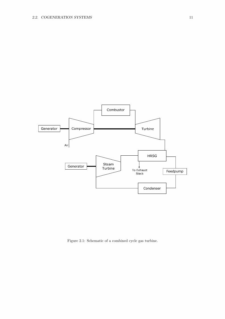
(CCP or CCPP). A simplified schematic of a basic CCGT layout is shown in Figure 2.1 where a
heat recovery steam generator (HRSG) replaces the fired boiler of the conventional steam plant.
The CCGT is possibly the most popular method used to recover waste heat from gas turbine
exhaust [26]. In recent decades many new plants have been constructed and existing plants re-
powered [27]. The popularity of CCGTs can be attributed to several advantages over existing
predominantly fossil fuel based power plants [28]. In particular CCGTs offer high efficiency, sig-
nificant emissions reductions, lower investment and operation costs, and greater flexibility in fuel
and plant operation [24, 29, 30, 28]. Furthermore, studies by Bolland and Stadaas [31], Heyen
and Kalitventzeff [32], and Carapellucci [33] have demonstrated that the CCGT generally achieves
better thermal efficiency over most comparable systems across a range of plant sizes.
Despite these advantages CCGT systems also posses several notable drawbacks. CCGT plants
represent greater complexity compared to individual gas turbine or steam plants as well as com-
parable advanced gas turbine systems, which is particularly problematic at smaller scales [33].
Additionally, despite a degree of operational flexibility, it is generally necessary to operate CCGT
plants at full load due to their poor part load performance [34, 27]. As a result considerations
of part load operation are often overlooked [35]. Furthermore, the increased interest in both grid
deregulation and distributed power generation, along with the increasing number of CCGT plants,
subjects these plants to a greater frequency of start-up and shut down operations [28]. Unfor-
tunately this cyclic behaviour leads to reduced plant lifetime [24, 28], along with the significant
economic and environmental issues of low efficiency and high NOx emissions during start up [36, 28].
2.2. COGENERATION SYSTEMS 11
Figure 2.1: Schematic of a combined cycle gas turbine.
12 CHAPTER 2. LITERATURE REVIEW
These issues have however motivated increased interest in applying advanced control approaches
to CCGT plants to mitigate some of these issues.
2.2.2 Combined Heat and Power
Combined heating and power systems represent the other most common application of cogener-
ation. These, as name indicates, are systems which produces both electrical and useful thermal
energy from the same primary source [19]. CHP systems have been demonstrated to reduce fuel
consumption by up to 30% compared to equivalent separate systems [37]. This is in addition to
the increased efficiency and significant emissions reductions (can be up to 50%) such systems give
[17].
The prime mover in CHP plants is typically either a gas turbine or reciprocating internal
combustion engine with the later generally being diesel based [37, 17]. However, gas turbines are
the most widely used due to their low complexity, low capital cost and flexibility [38]. While direct
heating from the exhaust gasses may be used it is more common to use steam generated by a heat
recovery steam generator (HRSG).
CHP systems have traditionally been used with large scale power plants and in industrial
applications [19], with the combined production of power and steam extensively used in the process,
paper, and food industries [39]. However the deregulation of electricity markets and subsequent
increase in distributed generation has lead to increasing popularity of CHP systems [19, 40, 41],
and an increase in small scale CHP systems [42, 19, 40].
2.2.3 Advanced Gas Turbine Cycles
The limitations, particularly in terms of scale, of conventional CCGT and CHP systems has mo-
tivated interest in alternatives. The advantages of gas turbines, namely low costs, low complexity,
high flexibility, and high reliability have ensured the gas turbine remains popular for power gener-
ation, particularly for small scale applications [33]. Hence, there has been considerable interest in
improving gas turbine performance through advanced cycles, in particular mixed-air steam cycles.
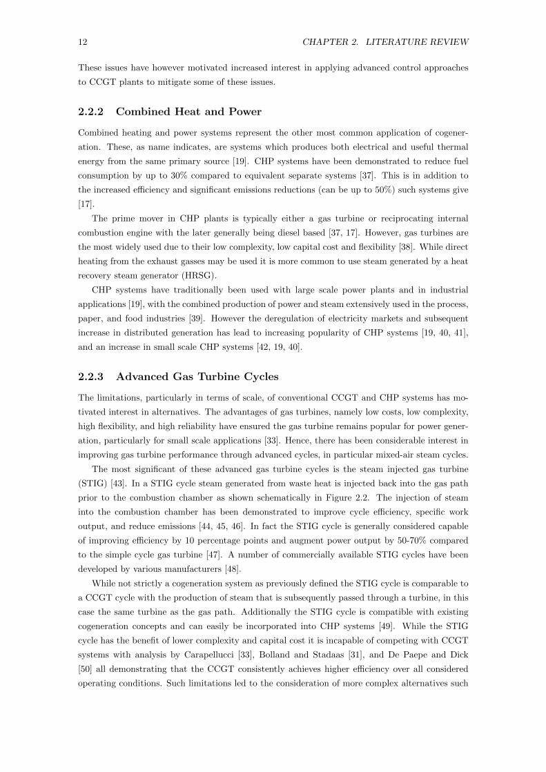
The most significant of these advanced gas turbine cycles is the steam injected gas turbine
(STIG) [43]. In a STIG cycle steam generated from waste heat is injected back into the gas path
prior to the combustion chamber as shown schematically in Figure 2.2. The injection of steam
into the combustion chamber has been demonstrated to improve cycle efficiency, specific work
output, and reduce emissions [44, 45, 46]. In fact the STIG cycle is generally considered capable
of improving efficiency by 10 percentage points and augment power output by 50-70% compared
to the simple cycle gas turbine [47]. A number of commercially available STIG cycles have been
developed by various manufacturers [48].
While not strictly a cogeneration system as previously defined the STIG cycle is comparable to
a CCGT cycle with the production of steam that is subsequently passed through a turbine, in this
case the same turbine as the gas path. Additionally the STIG cycle is compatible with existing
cogeneration concepts and can easily be incorporated into CHP systems [49]. While the STIG
cycle has the benefit of lower complexity and capital cost it is incapable of competing with CCGT
systems with analysis by Carapellucci [33], Bolland and Stadaas [31], and De Paepe and Dick
[50] all demonstrating that the CCGT consistently achieves higher efficiency over all considered
operating conditions. Such limitations led to the consideration of more complex alternatives such
2.2. COGENERATION SYSTEMS 13
Figure 2.2: Schematic of a Steam Injected Gas Turbine (STIG) cycle.
14 CHAPTER 2. LITERATURE REVIEW
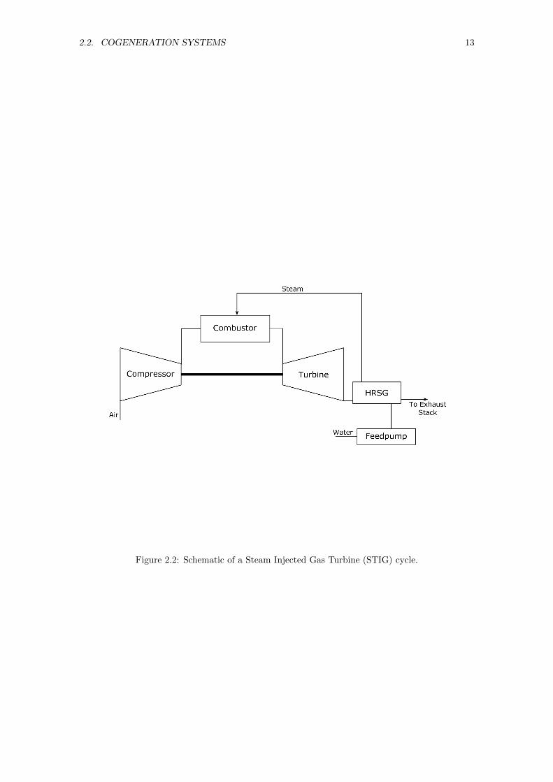
Country Percentage Industrial Electrical Consumption
USA [6] 10-16%
EU [58] 10%
Australia [59] 10%
Table 2.1: Proportion of industrial electrical consumption used for compressed air production.
as the DRIASI (dual-recuperated intercooled aftercooled steam injected) cycle which combined
recuperation, steam injection and water injection. Analysis by Bolland Stadaas [31] indicating
that such a cycle was competitive in efficiency terms with CCGT’s at small to medium scales.
Further variations on these principles and the related water injection concept have been considered
for improving gas turbine performance. These have many varied acronyms, such as HAT, ISTIG,
RWI, REVAP, CHAT, TOPHAT cycles. The STIG and CCGT cycles have also been proposed to
be merged into the combined STIG or FAST cycles [51, 48, 52]. However, commercial applications
generally appear to be restricted to simpler steam injection cycles. Nevertheless the use of advanced
gas turbine cycles such as steam injection offer benefits over the simple cycle and CCGT systems
with greater flexibility [39] and improved part load performance [48].
While mixed air-steam cycles generally demonstrate an acceptable trade-off between cost and
performance to make them competitive at smaller scales, they also have the disadvantage of high
water consumption, which can be a significant issue in areas with water shortages [53]. Fortunately,
both analytical and experimental studies, including those by De Paepe and Dick [54], Macchi and
Poggio [55], Xueyou et al [56], and Zheng et al [57], have determined that complete recovery of
water in a STIG cycle is possible. Additionally, these studies showed that the implementation of
water recovery is economically viable.
2.2.4 Further Industrial Applications
The most common implementations of gas turbine based cogeneration, along with advanced gas
turbine cycles, have received a considerable degree of attention, including well established com-
mercial implementations. However, the considerable attention given to these established systems
has lead to further alternative applications of cogeneration to be overlooked. In particular there
is relatively little consideration given to building on these existing systems for alternative applica-
tions. One such application is the cogeneration of two significant industrial resources, compressed
air and steam.
Compressed air production is a significant sources of industrial energy consumption and is
generally considered the ’fourth’ utility after electricity, gas, and water [4]. This is due to the
extensive applications of compressed air which include pneumatics, cleaning, cooling and more.
Compressed air is conventionally produced through electrically driven devices, most commonly
either screw or reciprocating compressors. This represents a significant proportion of industrial
electricity usage as shown in Table 2.1. Depending on the source of this electricity, compressed air
production can be a significant contribution to greenhouse gas emissions and operational costs.
An alternative to electrically driven compressed air production is the Gas Turbine Air Com-
pressor (GTAC) proposed by Wiese et al [9]. In this device a portion of air is bled off between the
compressor and the combustion chamber as a source of compressed air. Compared to conventional
compressed air production a GTAC device benefits from high power density, low vibration, and
2.3. CONTROL OF COGENERATION SYSTEMS 15
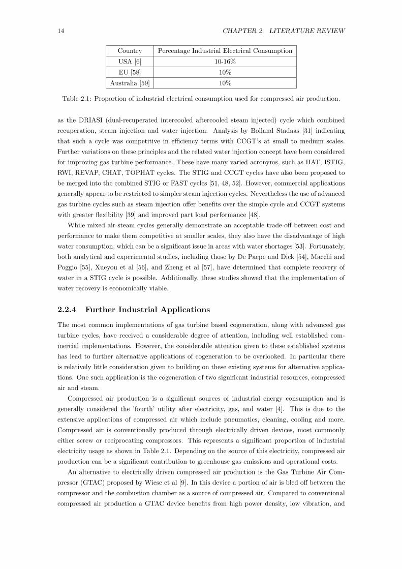
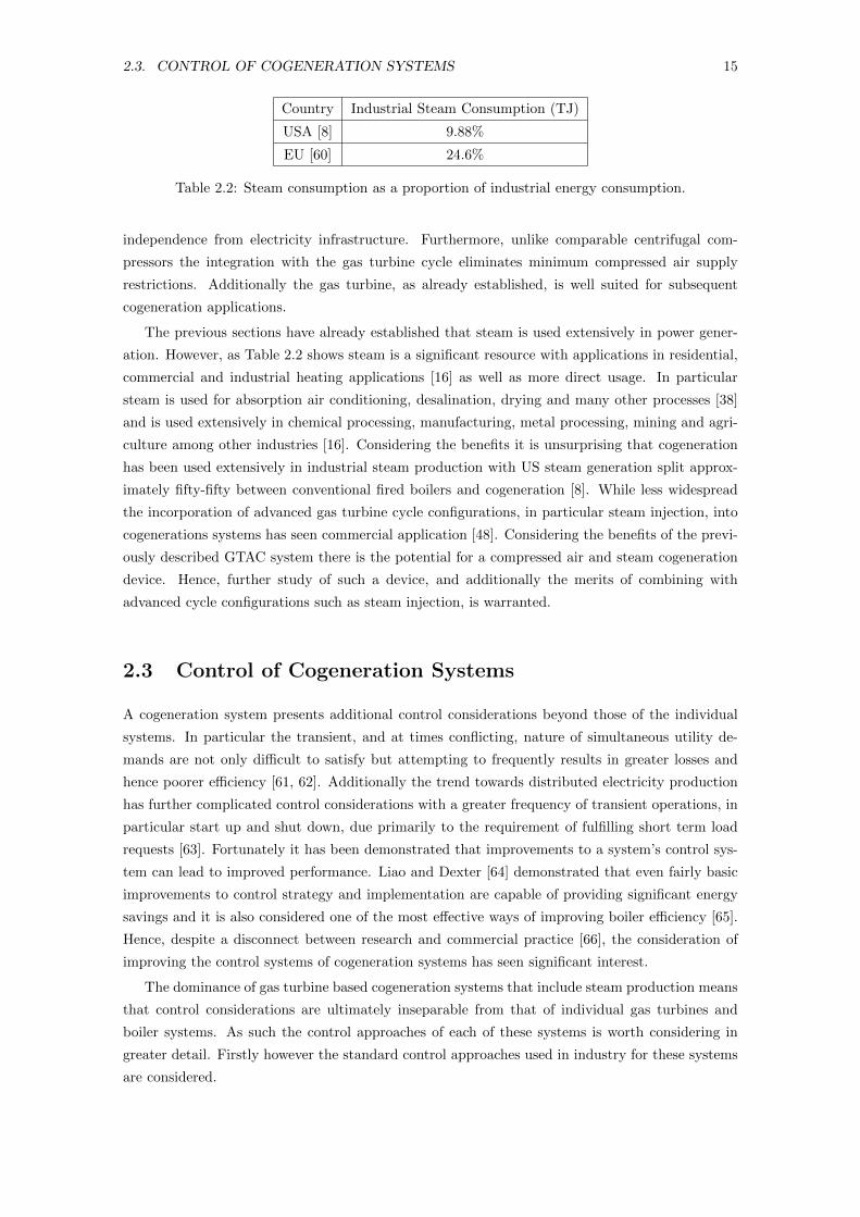
Country Industrial Steam Consumption (TJ)
USA [8] 9.88%
EU [60] 24.6%
Table 2.2: Steam consumption as a proportion of industrial energy consumption.
independence from electricity infrastructure. Furthermore, unlike comparable centrifugal com-
pressors the integration with the gas turbine cycle eliminates minimum compressed air supply
restrictions. Additionally the gas turbine, as already established, is well suited for subsequent
cogeneration applications.
The previous sections have already established that steam is used extensively in power gener-
ation. However, as Table 2.2 shows steam is a significant resource with applications in residential,
commercial and industrial heating applications [16] as well as more direct usage. In particular
steam is used for absorption air conditioning, desalination, drying and many other processes [38]
and is used extensively in chemical processing, manufacturing, metal processing, mining and agri-
culture among other industries [16]. Considering the benefits it is unsurprising that cogeneration
has been used extensively in industrial steam production with US steam generation split approx-
imately fifty-fifty between conventional fired boilers and cogeneration [8]. While less widespread
the incorporation of advanced gas turbine cycle configurations, in particular steam injection, into
cogenerations systems has seen commercial application [48]. Considering the benefits of the previ-
ously described GTAC system there is the potential for a compressed air and steam cogeneration
device. Hence, further study of such a device, and additionally the merits of combining with
advanced cycle configurations such as steam injection, is warranted.
2.3 Control of Cogeneration Systems
A cogeneration system presents additional control considerations beyond those of the individual
systems. In particular the transient, and at times conflicting, nature of simultaneous utility de-
mands are not only difficult to satisfy but attempting to frequently results in greater losses and
hence poorer efficiency [61, 62]. Additionally the trend towards distributed electricity production
has further complicated control considerations with a greater frequency of transient operations, in
particular start up and shut down, due primarily to the requirement of fulfilling short term load
requests [63]. Fortunately it has been demonstrated that improvements to a system’s control sys-
tem can lead to improved performance. Liao and Dexter [64] demonstrated that even fairly basic
improvements to control strategy and implementation are capable of providing significant energy
savings and it is also considered one of the most effective ways of improving boiler efficiency [65].
Hence, despite a disconnect between research and commercial practice [66], the consideration of
improving the control systems of cogeneration systems has seen significant interest.
The dominance of gas turbine based cogeneration systems that include steam production means
that control considerations are ultimately inseparable from that of individual gas turbines and
boiler systems. As such the control approaches of each of these systems is worth considering in
greater detail. Firstly however the standard control approaches used in industry for these systems
are considered.
16 CHAPTER 2. LITERATURE REVIEW
2.3.1 Industry Standard Control
2.3.1.1 Industry Standard Gas Turbine Control
Gas turbine applications, and their corresponding control requirements, fall in one of two categories.
The first is stationary gas turbines which are predominantly employed for power generation, where
the most important control requirement is regulating the shaft speed for varying loading conditions
since it is directly coupled to the generator [67, 61]. Hence, control of the shaft speed is equivalent
to control of the generator frequency which is necessary to be maintained constant under varying
load. The second category is propulsive gas turbines, used primarily in aircraft, most commonly
in the form of jet engines and turbofans. Here the primary control objective is to track a desired
thrust level defined by a commanded throttle position [68]. However, since thrust is not a directly
measurable quantity standard practice is to map the thrust to other measurable quantities such
as shaft speed or pressure ratio [68, 69].
While these form the main control requirements they are subject to a number of additional
constraints. The basic constraints require the gas turbine to operate within speed limits, pressure
limits, temperature limits, compressor surge/stall limits, and burner (blowout) limits in order to
both maintain correct operation and prevent either failure or significant lifetime reduction [68]. In
addition are the requirements to satisfy emissions and acoustic (for propulsive case) constraints
while maintaining a satisfactory level of performance [2]. Other constraints may be required where
additional equipment (such as recuperators) are present with the gas turbine. Furthermore, optimal
operation typically requires the gas turbine to be at or near one or more of these constraint limits
[68].
Gas turbines, in both stationary and propulsive capacities, are additionally subject to signifi-
cantly varying conditions. In the case of power generation this is primarily a result of load changes.
Such systems may also operate in regions of extreme weather variation and varying atmospheric
conditions [70]. For aircraft engines the change in conditions is a result of the wide operating
envelope of aircraft where significant changes in pressure, temperature and airspeed are experi-
enced through varying altitude and aircraft speed [2]. In addition both are subject to performance
degradation over the life of the device [2]. All of these makes the development of effective and
reliable gas turbine control systems quite challenging.
Mechanically speaking the primary control actuator in a gas turbine is the fuel flow actuator.
However, where present variable geometry, in the form of variable inlet guide vanes (VIGV),
variable stator vanes (VSV), and in the case of jet engines variable area exhaust nozzles provide an
additional control capability which can be used to maintain cycle efficiency at part load conditions
[67]. Closed cycle gas turbine systems, such as that proposed by Kikstra and Verkooijen [71], offer
similar capability by controlling the quantity and conditions of the working fluid in the cycle.
Historically the development of gas turbine control has been linked to the available hardware
capabilities at the time. Early gas turbine control was based on the hydromechanical control unit
(HMU). Essentially a mechanical computer these systems employ cams and mechanical integra-
tors to implement the required control system [68]. Constraint handling was generally performed
by independent devices for preventing the exceeding of speed and temperature limits as well as
avoiding blowout and other mechanical issues [72, 73]. Unfortunately HMUs were only capable of
implementing relatively simple control strategies [68]. While they were a reliable device the im-
plementation of more complex control systems on HMUs required a corresponding increase in size,
2.3. CONTROL OF COGENERATION SYSTEMS 17
weight, and expense beyond what was practical for aircraft control [73]. As such the early control
systems were essentially fuel governors to control the turbine speed that incorporated minimum
and maximum flow hard stops to prevent blow out and over temperature respectively [73].
The introduction of electronic control hardware did not occur until the late 1960’s [72] for
stationary systems and even later in the 1980’s [68] for aircraft engines. The implementation of
electronic control hardware for gas turbines required the development of sufficiently durable and
reliable electronic components and integrated circuits capable of surviving the harsh environment
they were required to operate in [68]. The early incorporation of electronics with aircraft engines
began in the 1970’s with existing HMU systems supplemented by supervisory electronic control
with both analog and digital electronic control units developed. However, the greater reliabil-
ity and flexibility of digital systems led to their adoption over analog systems [73]. Prominent
examples of the electronic systems developed were the Speedtronic series (the first electronic gas
turbine control unit) by General Electric for stationary systems [72] and the Digital Engine Control
(DEC) and Full Authority Digital Electronic Control (FADEC) by Pratt and Whitney and General
Electric Respectively [68]. The introduction of electronic control and the subsequent advances in
technology enabled the improvement of existing control approaches and provided significantly im-
proved diagnostic capabilities and overall engine reliability [68, 73, 74]. Furthermore, such systems
enabled the implementation of much more complex, advanced control approaches, although this
has generally seen much less implementation, particularly in aircraft engines, outside of research
[73].
While there will be some differences between the control requirements of stationary and propul-
sive gas turbines, and for that matter between turbofan and turbojet engines within propulsive
gas turbines, the overall control approach in commercial systems are comparable. Commercial
gas turbines have typically been controlled by a single closed loop fuel controller [68]. A repre-
sentative example presented by Garg [2] for a turbofan engine is shown in Figure 2.3. Here the
pilots command is mapped to a desired fan speed from which a fuel flow command is created by
a basic lead-lag compensator. The acceleration and deceleration schedules provide maximum and
minimum limits on the fuel flow primarily to prevent compressor stall, blowout and overstress of
the rotor. These schedules are defined in terms of a corrected core engine speed, NR2 , and the
ratio of fuel flow to combustor inlet pressure, Wf/Ps30, with Figure 2.4 showing how these protect
the engine. The resulting command is passed through additional Min/Max control architecture to
ensure commanded fuel flow stays within additional limits such as overspeed.
The main control element itself is implemented with basic PI control, where the gains were
determined via linear models and scheduled over a range of operating conditions [2, 69]. The
design of these controllers was generally based on standard SISO techniques and successive loop
closure techniques, the later being the standard approach in industry to decouple effects among
multiple controlled variables [73]. As previously indicated additional actuators may be present
in the form of VIGV, VSV, and other systems providing additional control actuation. However,
these systems generally don’t form part of the main control loop and are instead used for further
ensuring safe operation of the engine and may also be used to maintain efficient operation as well
[2, 67].
While the gain scheduled PI control approach is well established and has been the predominantly
used approach in commercial gas turbines it also suffers from several significant disadvantages over
modern control approaches. Most significantly is that this approach essentially applies linear SISO
18 CHAPTER 2. LITERATURE REVIEW
Figure 2.3: Example of standard fuel control structure for a turbofan engine [2].
Figure 2.4: Representative diagram of acceleration and deceleration schedules intended to protect
engine [2].
2.3. CONTROL OF COGENERATION SYSTEMS 19
control approaches to what is a highly nonlinear MIMO system. Additionally, the performance of
the gain scheduled PI based controller is dependent on the the quantity and range of operating
conditions used to set these gains. It cannot be definitively guaranteed that a gain scheduled
controller will meet performance requirements at off-design operating conditions [75]. Furthermore
the enforcement of gas turbine operational limits are very conservative due to both the necessity
of implementing them through separate systems and the incapability of adapting to the changes
resulting from the general wear and deterioration of the engine. As such, gain scheduled PI control
is ultimately a suboptimal control approach for a gas turbine.
2.3.1.2 Industry Standard Thermal Plant Control
The control of boilers is largely inseparable from that of the thermal plants they are most commonly
part of. As such the attention given in research for control of boilers predominantly concerns those
that form part of thermal plants. Ignoring supercritical plants, which are beyond the scope of this
thesis, this mostly concerns the standard drum type boiler shown in Figure 2.5. While other boiler
configurations exist the control of the drum boilers has been the area of most interest.
In the case of power plant applications it is generally desired to supply the required power
output while simultaneously maintaining optimal plant efficiency and integrity [66]. To this end
it is necessary to maintain steam temperature and pressure values at desired levels in the face of
load or demand variations [66, 76]. In particular controlling the pressure in the evaporator (or
riser) ensures thermal energy stored within the evaporator remains within acceptable limits [77].
Additionally it is necessary to maintain the water level in the drum to ensure both correct and
safe operation of the plant [66]. Depending on the heat source for the boiler (combustion, nuclear,
etc.) additional constraints may be required for the combustion conditions to ensure efficient
operation and to meet environmental requirements [66, 76]. Of particular importance is ensuring
thermal stresses within the major components remain within acceptable limits as excessive thermal
stress can significantly reduce the lifetime of the component [77, 63, 36]. This is generally realised
through rate of change constraints and is of most significance during startup/shutdown operations
[78]. Beyond these major requirements and constraints are the general limits on components and
actuators operating ranges, in particular the limits on the feedpump operating range [79].
Like the conventional control approach for gas turbines discussed previously the control for
boilers in thermal plants is based on well established SISO methods with more advanced modern
control approaches generally not considered in commercial plants [66, 77]. The typical boiler
control system is built from multiple independent regulation loops and feedforward compensators
[66, 77]. These regulation loops are based on PID controllers with additional parameter scheduling
also incorporated into the control system [80]. In typical thermal power plant operations the boiler
is operated in one of three modes. The first of these, which is used during normal operation of
the plant, is called boiler following mode [77]. In this mode the turbine governor valve (a valve
upstream of the turbine) is used to control the plant load while the boiler heat source (usually firing)
is adjusted to maintain boiler pressure [77]. The second mode is called turbine follow mode and is
normally used to ensure plant safety [77]. Here the turbine governor is instead used to maintain
boiler pressure while adjustments to boiler firing is used to meet plant load demand [77]. The
third mode is called sliding pressure mode. In this mode the pressure is permitted to slide within a
range of values which allows for smoother plant operation [77]. The boilers of cogeneration plants,
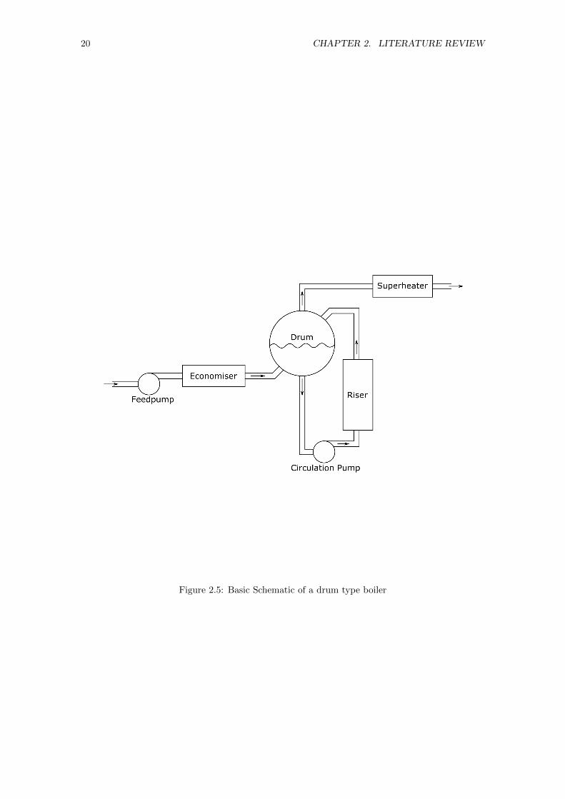
20 CHAPTER 2. LITERATURE REVIEW
Figure 2.5: Basic Schematic of a drum type boiler
2.3. CONTROL OF COGENERATION SYSTEMS 21
in particular CCGT plants, despite the addition of the gas turbine have generally been controlled
by the same general process as standard thermal plants [81]. It would be expected that the specific
gas turbine control in such plants would follow the processes described previously.
As with the standard approach to gas turbine control described previously the conventional
approach to boiler control and the control of thermal plants in general has a number of drawbacks.
Beyond the limitations already established previously in the context of gas turbine control, it is well
established that with the changing nature of power generation, in particular with changing demand,
fuel variations, and general deterioration of boiler surfaces, the PID based control approach of
thermal plants does not achieve a high level of performance [81, 82]. Furthermore, the necessity
of incorporating decoupling techniques and other approaches to account for the nonlinear and
highly cross-coupled reality of a boiler penalises performance resulting in slower dynamic behaviour
[81, 82, 77]. While, satisfactory performance is generally obtained under normal plant operations
the penalty to performance can be quite severe in emergency situations or where sharp changes
in demand occur, potentially leading to significant oscillatory behaviour and subsequent reduction
in lifetime [77]. The deregulation of the electricity market additionally increases the likelihood of
such occurrences.
2.3.2 Model Predictive Control
The advancing capabilities in the available hardware lead to increased research interest in advanced
control approaches for gas turbines [73] and thermal plants [77]. The most popular modern control
approaches examined were based on the linear quadratic regulator (LQR) and H∞ control methods.
The basic LQR approach has seen extensive research for gas turbine control [83, 84, 85, 86] along
with variations like the Linear Quadratic Gaussian/Loop Transfer Recovery (LQG/LTR) approach
[87, 88, 89]. These approaches have seen similar application to boiler and thermal plant control
[90, 91, 62, 92]. H∞ control approaches have also been widely demonstrated for both gas turbine
[93, 94, 95, 96, 75, 97] and thermal plant control [98, 99, 100].
While both LQR and H∞, along with their respective variations, offer significant improve-
ment over the existing industry standard for both gas turbine and boiler control there are still
two significant drawbacks. Firstly these approaches are predominately based on linear methods
and linearised models requiring gain scheduling or equivalent approaches, thus limiting controller
robustness and requiring conservativeness in controller design. Secondly, these approaches still
require constraints to be enforced separately leading to further conservativeness in controller de-
sign. As such, both approaches, while improved, still ultimately result in suboptimal control. A
control approach that has seen increasing interest which is capable of overcoming these drawbacks
is a form of model-based control called model predictive control (MPC). In MPC a model of the
plant is used to optimise an open loop control trajectory over a finite time period. Specifically,
the control action is determined by solving a finite horizon optimal control problem for the current
state to obtain an optimal control sequence [101]. Assuming a discrete time system this optimal
control problem can be described by:
arg minU,x
J =
Np−1∑j=0
Cj (x (tj) , u (tj) , yr (tj)) + Cterm(x(tNp))
(2.1)
subject to : G (x, u) = 0 (2.2)
22 CHAPTER 2. LITERATURE REVIEW
H (x, u) ≥ 0 (2.3)
where the discrete control sequence U is defined as
U = [u (t0) , u (t1) , ...u (tNctrl)] (2.4)
where only the first element is normally used for the next control input to the plant. Np and Nctrl
refer to the prediction and control horizons respectively while x and yr are the state vector and
reference trajectory respectively. The vector functions G and H define the equality and inequality
constraints of the optimisation problem respectively, noting that the equality constraints include
the equations describing the plant model and the inequality constraints primarily represent the
operating limits of the plant. The terms of the objective function J are the stage costs Cj and
the terminal cost Cterm, the latter of which normally forms part of the stability analysis of the
controller [102]. By using only the first control input and reevaluating the optimisation for each
sampling instant MPC effectively acts as a closed loop controller despite not incorporating direct
feedback. The basic MPC approach presented here offers several advantages over the current
commercial control approach and other modern control approaches. Firstly, the operational limits
of the plant can be directly considered in the open loop optimisation through the constraint terms G
and H. Secondly, it is capable of handling MIMO systems without the need for decoupling unlike
the existing PI approaches. Thirdly, competing objectives can be more easily handled through
either the objective function or constraints. Hence, MPC has seen growing interest in applications
for both gas turbines and boilers, including in cogeneration plants. The primary drawback of
MPC is the increased computational complexity resulting from the optimisation process. As such
implementation of MPC for cogeneration and related systems has largely focused on methods for
mitigating this drawback. This has mostly focused on methods for implementing considerably
more computationally tractable linear MPC methods, the use of computationally simple models,
or alternative approaches to implementing MPC.
2.3.2.1 MPC Gas Turbine Control
While gas turbines are highly non-linear the computationally simpler and better established linear
MPC, where linear models are employed, has seen reasonable attention for gas turbine control.
Linear MPC implementations have been examined by Lyantsev et al [103, 104], Ghorbani et al
[105], and Ailer et al [106] for regulation problems around particular set points. Under these cir-
cumstances where the transients are small and the objective is to maintain operation around a
particular operating condition the use of linear MPC is quite reasonable. However, under large
scale transients linear MPC, like the approaches covered previously, may suffer from degradation
of performance and stability. Hence, the application of non-linear MPC (NMPC) has seen consid-
erable attention, with a significant focus in overcoming the increased computational complexity of
NMPC to make the controller practical to apply.
The most commonly considered approach is that of successive linearisation where the nonlinear
plant model is linearised at each sampling instant allowing linear MPC methods to be used. This
approach has been examined by Vroemen et al [107] in simulation for a small laboratory scale
stationary gas turbine including comparisons with hybrid linear and nonlinear approaches. This
successive linearisation approach was subsequently validated experimentally by van Essen et al
2.3. CONTROL OF COGENERATION SYSTEMS 23
[108] demonstrating good performance for relatively slow sinusoidal transients (period of 150s).
While some excursions outside of temperature constraints were observed these were considered to
be due to the insufficient speed in the filter being used to deal with model mismatch. Additionally,
hardware limitations restricted the controller to a sample time of 1.2s. As such the ability of the
controller to respond to more severe commands or disturbances is uncertain. Further examples
of successive linearisation have been demonstrated in simulation by Brunell et al [109] and Mu
et al [110] for aircraft engines using different modelling approaches. In the case of Brunell et al
[109] a physics-based nonlinear component level model is used with the successive linearisation
performed by a first order Taylor’s series expansion. An extended Kalman filter is additionally
incorporated into the system to estimate the unmeasurable states. Unlike Vroemen et al [107] and
van Essen et al [108], Brunell et al [109] only considers steady state operation as a test case for
maintaining engine performance following deterioration of the engine. However, in the simulations
it is assumed that the NMPC model is very close to the engine model eliminating the effect of
plant model mismatch. Mu et al [110] on the other hand uses a neural net based gas turbine model
as the prediction model. While these cases demonstrate that successive linearisation improves
on existing control strategies, and in the case of [107] demonstrates superior behaviour to linear
MPC, successive linearisation compromises on model accuracy and feasibility compared to a fully
nonlinear approach. Furthermore, aside from the experimental demonstration by van Essen et al
[108], the real time implementation of the controllers is not examined making it uncertain if these
presented approaches could feasibly be implemented on actual plants.
An alternative approach to reduce the computational complexity of NMPC was examined by
Richter et al [111] with multiplexed MPC (MMPC). Here computational complexity is reduced
by only considering a subset of the control actuators at each sampling instant, though it should
be noted that successive linearisation was still employed to further reduce the complexity. The
resulting controller showed acceptable performance and significantly reduced computation time
compared to a fully nonlinear MPC approach. While stability is discussed in terms of a linear the
system the authors note that further work is required to establish the stability conditions of the
multiplexed plant.
Another approach receiving considerable attention is to use non physics-based models that are
either simpler or include properties that can be exploited for reduced computational complexity.
Jurado et al [112, 113] employs Hammerstein models for the prediction model. Since the Ham-
merstein models are constructed as single output systems the inversion of the nonlinear map part
of the model is relatively simple. Furthermore, a property of Hammerstein models means that
this inversion results in a linear system allowing linear MPC approaches to be used. Jurado [112]
demonstrated that this approach was able to give superior performance compared to straight linear
MPC. However, the real time implementation of the approach is not examined making it unclear
if the approach is viable for actual implementation. A similar approach is employed by Diwanji
et al [114] with models of the Weiner-Laguerre-ANN structure which divides the model into a
linear dynamic section and a nonlinear map for states to outputs constructed by neural network
methods. Unlike Jurado et al[112, 113] Diwanji et al applies explicit NMPC and achieves good
tracking of the reference signal. However, the only constraint considered is on the turbine inlet
temperature making it uncertain if the implementation would be practical in a real application.
Furthermore, an assessment of real time implementation is not considered. An alternative model
type considered by Brunell et al [115] was a simplified real time gas turbine model developed by
24 CHAPTER 2. LITERATURE REVIEW
Shaoji [116] based on transfer functions representing the state dynamics with nonlinear algebraic
equations describing the outputs. Extended Kalman filtering was additionally employed to obtain
all the required states. While the controller demonstrated acceptable performance the authors
were unable to implement the controller in real time and the maximum error between the simpli-
fied model and a corresponding high fidelity model reached 22% which was considered outside the
limits of acceptable accuracy.
While data driven models, such as those above, are often easier to develop from input-output
data, this loses the physical meaning present in physics-based models. This can be resolved by
using computationally simpler versions of physics-based model. This has been demonstrated ex-
perimentally by Wiese et al [117] who implemented fully nonlinear online MPC on a small scale
gas turbine using a reduced order physics-based model as the prediction model. Hence, Wiese et al
[117] was able to demonstrate that it was possible to implement NMPC on a gas turbine without
requiring linearisation. Furthermore, the implemented control system demonstrated the advan-
tages of MPC for gas turbines with constraint handling and disturbance rejection while achieving
minimal response times.
2.3.2.2 MPC Boiler and Thermal Plant Control
Compared to gas turbines the slower dynamics and rate of change restrictions make thermal plants a
more promising application for nonlinear MPC. A straightforward application of MPC to a 320 MW
oil fired plant has been considered by Poncia [77] where it was assumed that the plant predominately
operated at full load and as such a linearised model about this point was used. The resulting
controller demonstrated improvements over conventional control and identified several advantages
over this. In particular reduced thermal stress on components and reduced stress on actuators were
observed which would extend the life of plant components. However, as the linearised model was
restricted to a full load operating condition, significant deviations from this operating point could
not be conisdered. This concept is extended further by Prasad et al [118] with the implementation of
successive linearisation with an extended Kalman filter used to determine minimum variance state
estimates in each sampling interval. Additionally the controller incorporated online estimation
of time varying model parameters enabling better handling of associated disturbances. However,
since both cases employed some degree of linearisation the same restrictions as found previously
for gas turbine control apply with successive linearisation compromising on accuracy. Horalek
and Imsland [76] however demonstrated that fully nonlinear MPC can be implemented to control
a typical boiler using an optimisation algorithm based on the simultaneous direct collocation
problem formulation and interior point optimisation. Furthermore, the controller was assessed
to be sufficiently computationally efficient to be real-time implementable. However, the NMPC
implemented was relatively basic with the authors indicating that further consideration of integral
control, adaptivity, time delays and stability would be required.
Considering the demonstrated usefulness of MPC for gas turbines, boilers, and thermal plants
in general this control approach has seen a reasonable degree of attention for cogeneration with
CCGT plants given considerable attention. In particular, significant attention has been given
to attempts to improve the start up process of CCGT plants. While not strictly MPC, similar
model-based optimisation methods have been examined in simulation by Albanesi et al [28] and
Shirakawa et al [119] for CCGT start up. In both cases the start up times of the plants were
2.4. TRANSIENT MODELLING OF COGENERATION SYSTEMS 25
significantly reduced while maintaining safe operation demonstrating the merits of these types of
approaches. However, both cases considered only simulation results making it unclear if either is
suitable for online implementation. The use of MPC in CCGT start up has been demonstrated by
D’Amato [36] on a 480 MW CCGT plant at Baglan Bay in South Wales. This was achieved by
the development of efficient large scale QP algorithms for highly structured data along with the a
linearisation approach that linearised the model at each step in the cost function evaluation. As
with the previous cases the controller demonstrated a significant reduction in start up time along
with reductions in both fuel consumption and NOx emissions. While these cases demonstrate the
usefulness of MPC for start up procedures, these are traditionally the slowest and most dynamically
restricted operations of the plant. As such it is unclear how these approaches would extend to more
general power plant operation.
Beyond start up improvements nonlinear MPC has been demonstrated in simulation by Aurora
et al [27] for regulation applications. Specifically Aurora et al examined regulation of steam
temperature and gas turbine flow rate in addition to examining efficiency optimisation at part
load. The resulting controller demonstrated improvements in steam control over conventional
PID approaches in addition to significant fuel savings at part load conditions. However, since
the controller was only applied to a subsystem of the plant it was found to inadvertantly produce
stronger oscillations in the drum level. As such, partial implementation of MPC may be unsuitable
for cogeneration systems.
A comparison of these modern control approaches, that is LQR, H∞, and predictive methods,
has been considered by Nakamoto et al [120] which was able to demonstrate that, as might be
expected, all of the modern approaches demonstrated improvements over conventional PID based
control. While comparable performance was observed for all three controllers near the identification
data set, the predictive controller demonstrated robustness over a wider operating range achieving
excellent tracking over a start up procedure. Hence, predictive methods, such as MPC, are likely to
offer advantages over other multivariable control methods such as LQR and H∞. Especially when
the ability to inherently account for constraints is also considered. While MPC does not receive
the same degree of attention in other cogeneration systems as it receives in CCGT systems it would
be expected that comparable benefits would be possible. It is apparent however that further study
of the actual implementation of MPC control on actual plants over a range of operating conditions
is required.
2.4 Transient Modelling of Cogeneration Systems
It has been established that MPC offers a number of benefits for the control of cogeneration
systems. However, the effectiveness of MPC is dependent on the model used, with a need for a
suitable level of accuracy combined with sufficient computational efficiency. As indicated in the
previous section this computational efficiency is frequently achieved through the use of linearisation
or through very simple, usually empirical, models, thus compromising on accuracy. Considering
that a wide variety of both gas turbine and boiler models have been developed there is scope for
identifying more suitable models or modelling approaches. These can range from very detailed three
dimensional models to highly simplified models consisting of only a few states. Considering that
the computational complexity of the former typically leads to them being unsuitable for control
considerations this examination will primarily focus on those suitable for use with model-based
26 CHAPTER 2. LITERATURE REVIEW
control or appropriate for model reduction to a suitable form.
2.4.1 Gas Turbine Modelling
The limited computing capability of the time restricted early gas turbine models to relatively simple
linear models such as those by Otto and Taylor [121] and Ketchum and Craig [122]. These early
approaches incorporate the assumption of quasi-steady thermodynamic and fluid flow properties
with the shaft dynamics defined as simple linear models of the fuel flow rate and shaft speed.
The associated coefficients are determined from steady state characteristics. While the models
correlated well with data in the vicinity of the selected steady state operating conditions, away
from these conditions, and in particular during acceleration and deceleration transients, the models
generally performed poorly.
As computational capability improved the interest in nonlinear models capable of representing
the gas turbine over it’s full range of operation increased. Since techniques such as successive lin-
earisation would permit well established linear control methods to continue being used this interest
included control-oriented nonlinear models. While early nonlinear models continued to build on
existing concepts, such as the continued use of assumed quasi-steady thermodynamic and fluid
flow properties by the nonlinear model of Mueller [123], subsequent gas turbine modelling divided,
broadly speaking, into two main categories. The first, which have been popular in controller devel-
opment, are phenomenological models which at the simplest level construct input-output relations
often based on general model identification techniques. The second are physics-based models, like
those presented above, where the models are constructed from the fundamental equations describ-
ing the physical phenomena of the system (eg. mass, momentum, and energy conservation).
2.4.1.1 Phenomenological Models
The development of phenomenological models was motivated primarily by the desire for simpler,
more computationally efficient models suitable for us with control applications. The most com-
mon form of phenomenological modelling was the construction of transfer functions describing the
relevant system dynamics as demonstrated by Rowen [124], Zhang and So [29], and Mantzaris and
Vournas [125]. These included transfer functions describing the dynamics of actuators and control
systems. However, these models were fairly simple and treated the gas turbine, with the excep-
tion of the rotor dynamics, as a linear nondynamic system with the corresponding restrictions in
applicable range. The model by Rowen [124] in particular is limited to a valid range of 95-107%
of the rated speed. As such these types of models are of limited usefulness for excursions far from
the plant’s nominal operating point.
Methods for extending the range have been examined by Ahlbeck [126], Hung [127], and
Lichtsinder and Levy [128] for models where the transfer functions are constructed from lead-
lag models describing the gas turbine dynamics. Here the the time constants and sensitivities of
the lead lag models are scheduled as functions of the operating conditions in a similar manner to
the gain scheduling approach used for extending linear control approaches described previously.
While Ahlbeck [126] scheduled the time constants against power output and the gains against
open loop steady state characteristics, Hung [127] achieved better results by scheduling against
engine speed. A more complex approach was taken by Lichtsinder and Levy [128] with scheduling
against altitude, Mach number and fuel flow using modified generalised describing function meth-
2.4. TRANSIENT MODELLING OF COGENERATION SYSTEMS 27
ods. However, as with gain-scheduling this approach is limited to the valid operating range of the
time constant data. Furthermore, representing the dynamics of the system by only a few specific
time constants can lead to additional potentially significant dynamics being omitted or possibly
merged into other dynamics.
An alternative approach for describing the transfer functions through multisine signals coupled
with frequency domain techniques as part of a model identification process applied to either em-
pirical or model data has been considered by Evans et al [129, 130, 131, 132] and Arkov et al [133].
While demonstrated to be more effective than standard system identification techniques, this is at
the expense of more complex and potentially more time consuming data collection. Furthermore,
it is still, like the previous phenomenological models, based on linear models and subject to the
limitations therein. In particular the limited range of applicability around the data sets used for
fitting the models.
To overcome the limitations of using linear models a nonlinear phenomenological modelling
approach called Nonlinear AutoRegressive Moving Average with eXogenous inputs (NARMAX)
has been demonstrated by Basso et al [134], Boaghe et al [135] and Chiras et al [136] for modelling
of gas turbines. The NARMAX modelling approach constructs nonlinear functions, F , of the form
y(k) = F [y(k − 1), ..., y(k − ny), u(k − 1), ..., u(k − nu), ξ(k − 1), ..., ξ(k − nξ)] + ξ(k) (2.5)
where u and y are the input and output signals respectively with ξ accounting for noise and
uncertainties. The terms ny, nu, and nξ denote the maximum lagged values for the outputs,
inputs, and noise signals respectively. The actual form of the nonlinear function F varies, with
polynomial, rational function, radial basis functions, and wavelet decompositions among the more
popular choices [135]. While able to provide a more detailed model than the previous methods
this is at the expense of a more complex model and fitting process.
While the phenomenological modelling approaches provide models that are generally more
computationally efficient and built from well established system identification processes they lack
representation of the physical behaviour of the system. While this is not strictly required for a
control application this limitation, along with the more common use of linear models, restricts the
valid range of the model to the available data. Hence a significant spread and density of steady
state and dynamic data is required to ensure the model is adequately representative of the system.
In highly nonlinear system with regions in which severe behaviour can occur, such as for a gas
turbine near the system constraints, the use of phenomenological models can be a liability requiring
greater conservativeness in the controller development.
2.4.1.2 Gas Turbine Physics-Based Models
When considering physics-based gas turbine models suitable for control applications, which in this
case is nonlinear one-dimensional models, the models can generally be divided into two types.
These are the intercomponent volume (ICV) models and those of the direct numerical simulation
approach.
2.4.1.2.1 Intercomponent Volume Models
28 CHAPTER 2. LITERATURE REVIEW
The principle behind intercomponent volume models (ICV), as described by Schobeiri et al
[137] and Camporeale et al [138, 139], is for the compressor and turbine to be treated as compact
components without volume. These are separated by control volumes (or plena) that act as coupling
components and account for the dynamic behaviour of the system. This considers the unsteady
mass balance and the unsteady energy balance behaviour as well. The compact components are
typically modelled using their steady state characteristics.
Early versions of the ICV approach have been presented by Fawke and Saravanamuttoo [140],
Sellers and Daniele [141], and Daniele et al [142]. Fawke and Saravanamuttoo demonstrated how
the ICV approach improved steady state iterative approaches that were used at the time. However,
as these early approaches were mostly built upon the use of these steady state iterative approaches,
mitigating the benefits of the ICV approach.
Subsequent models built on these principals with various improvements and additions. Cam-
poreale et al [138, 139], da Cunha Alves and Barbosa [143], Martin et al [144], and Traverso [145]
incorporated forms of heat transfer. In particular [138], [143], and [145] included heat exchanger
modelling to examine recuperated gas turbine cycles while [139] developed a more detailed ap-
proach to modeling blade cooling in the turbine. Turbine blade cooling was also incorporated into
the model by Chacartegui et al [146] with the further addition of plena between compressor and
turbine stages to incorporate unsteady compressor and turbine dynamics. Martin et al [144], while
not considering blade cooling, did incorporate consideration of the effects of heat soakage on the
turbine. Other improvements to this modelling approach were considered by Crosa et al [147]
with a more detailed combustion model, including consideration of CO and NOx emissions. Other
authors such as Kolka et al [148] and Traverso [145] have included additional dynamic components
such as generators.
While the ICV modelling approach has seen extensive use, including with control system design,
it has the drawback of requiring characteristic maps for the static components. While this is fairly
straightforward for an operating device if appropriate data is available, this does restrict the
model to the range covered by these maps. Hence, the ICV modelling approach can be limited
when off-design operation is considered. Furthermore, during the design phase of the system such
information is not available without detailed modelling. An alternative approach was examined by
Schobeiri [137] with the inclusion of dynamic mass, momentum, and energy conservation equations
into the conventionally static components. While the simulation results showed that the model
was capable of representing complex engine configurations, it is unclear what effect including these
dynamics with the ICV plena will have. Additionally, such an approach mitigates the benefits of
the ICV modelling approach, such as the elimination of these dynamics.
2.4.1.2.2 Direct Numerical Simulation Models
The most common form of the direct numerical simulation approach is the solving of the
conservation of mass, momentum, and energy differential equations numerically over the discretised
domain of the system. The discretisation of the system flow path permits the governing partial
differential equations to be converted to a a set of ordinary differential equations typically through
either finite differencing or a finite volume approach. This approach is well described by Ricketts
[149] using a standard 1D differential form of the conservation equations. In forming the set of
governing equations the most commonly used form of the state vector is defined as density, density
2.4. TRANSIENT MODELLING OF COGENERATION SYSTEMS 29
flux, and energy as demonstrated by Owens et al [150, 151] and Kim et al [152, 153].
The division of the flow path into a series of finite elements permits a higher spatial resolution
of the individual components allowing for a more accurate representation of the system. This
has been taken advantage of by Kim et al [152] and Kikstra and Verkooijen [20] to produce more
detailed models. Kim et al [152] implements a stage by stage calculation process for the compressor
and turbine models, including consideration of VIGV and VSV, with generalised experimentally
determined characteristic curves to predict the performance of each stage. Kikstra and Verkooijen
[20] on the other hand use a staggered grid of flow nodes and thermal nodes for the finite element
scheme with the compressor and turbine modelled by a more fundamental approach based on
work by Gravdahl and Egeland [154]. However, while these models are able to describe the flow
path in greater detail with higher resolution they are also subject to greater computational cost
which can be prohibitive where control applications are intended. Furthermore, it is difficult to
adopt standard characteristic maps, in particular those of the compressor and turbine, to this
type of detailed finite element approach as shown by [152] and [20] were alternative more complex
approaches were required. As such, while these more detailed approaches are of benefit for dynamic
studies they are generally unsuitable for control application without further model reduction.
An alternative approach to permit the use of standard characteristic maps, and thus simplify the
model development, is to construct the finite elements such that they correspond with component
boundaries as demonstrated by Korakianitis et al [155] and Kim et al [153]. While this leads to a
less detailed coarser representation of the system it is simpler to set up and more computationally
efficient. Unlike the ICV models, which also commonly use characteristic maps, the dynamics of
the components are retained. While appropriate for dynamic studies, neither Korakianitis et al
[155] nor Kim et al [153] were considering control applications in the development of the models.
As such further examination of the suitability of the approach is required.
An approach that further builds on this idea, and ultimately with control applications con-
sidered, was developed by Badmus et al [13, 14, 15] for a non-dimensional framework based on a
state vector defined as Mach number, non-dimensional stagnation pressure, and non-dimensional
entropy. Here the source terms for the governing differential equations, which are themselves de-
fined in terms of influence coefficients, are defined in functional terms of steady state characteristic
maps for all components offering significant computational improvement over many comparable
models. Furthermore the structure of the modelling framework is well set up for model reduction
by singular perturbation and time scale separation arguments permitting the development of a
form appropriate for model-based control. An alternate form of model has also been developed by
Puddu [156] with non-dimensional entropy replaced by non-dimensional stagnation temperature.
The framework developed by Badmus et al [14] was further extended and validated experimentally
for a small scale gas turbine application by Wiese et al [3]. While the computational complexity of
model did not permit direct application to model-based control the structure was well suited for
formal model reduction. With the application of model reduction a low order form of the model
was developed and succesfully implemented in an MPC controller for the same small scale gas
turbine [117]. Hence, this modelling approach has demonstrated sufficient accuracy combined with
the required computational efficiency for use with model-based control applications and as such is
worth consideration for use with a cogeneration application.
30 CHAPTER 2. LITERATURE REVIEW
2.4.2 Boiler Modelling
Similarly to gas turbine modelling, boiler models can generally be divided between phenomenolog-
ical and physics-based models. However, possibly due to the typically slower dynamics of boilers,
physics-based models have seen more extensive use in both general simulation and control appli-
cations compared to gas turbine modelling.
2.4.2.1 Boiler Phenomenological Models
As with the case of phenomenological models for gas turbines, those for boilers have been primarily
motivated by the desire for relatively simple, easily fitted, computationally efficient models for ei-
ther control applications or to operate with the limited computational capability of early hardware.
The earliest attempts at these types of models, such as that by Astrom and Eklund [157] were
built around representing a small number of core dynamics. In the case of [157] this was a single
nonlinear differential equation for the drum pressure related to the difference in input and output
power of a boiler-turbine unit with output power the primary model output. The parameters of
this model were determined from a combination of physical arguments and experimental data. As
might be expected these early models generally lacked the detail to fully describe the behaviour of
a system as complex as a boiler.
Subsequent phenomenological boiler models followed a similar concept but constructed the
models from the more recognisable dynamics of the wall thermal inertia and the storage dynamics
of the large volumes present in boilers. As demonstrated by Cheres [158] and Zhang and So [29]
this permitted the model to be constructed from easily determined time delay and time constant
information. In the case of Cheres [158] the model was based on a low order two port network with
the dynamics defined by a fuel time delay, fuel and riser time constants, and a storage constant
for the boiler. Zhang and So [29] on the other hand reduced the model to single transfer function
incorporating time constants for both the boiler metal and storage dynamics. Similar models based
on boiler time constants have also been developed by Xu et al [79] and Kim et al [92]. However,
these modelling approaches are restricted to the valid ranges of the time constant used. Cheres
[158] in particular notes that the standard deviation in these model parameters can be as high
as 50% depending on the application. Furthermore, while the empirical nature of acquiring time
constants leads to representative dynamics of the system, potentially important dynamics are not
always considered. Zhang and So [29] for example consider the relatively important dynamics
associated with the thermal inertia of the boiler whereas these are omitted by Cheres [158] and
Kim et al [92].
Alternative approaches to the use of time constants built around linear modelling have been
examined by Rossiter et al [78] and Nakamoto et al [120]. Rossiter et al [78] used experimental
data, specifically step response data, to construct a continuous time linear model built around four
transfer functions mapping the plant inputs, firing rate and governor valve position, to the outputs
of pressure and power. Nakamoto et al [120] constructed the model in the form of an ARX model,
which is the linear model version of the NARMAX approach which has been mentioned previously
for gas turbine modelling.
While each of these models of the phenomenological approach were generally able to com-
bine adequate accuracy with computational efficiency they are subject to the same drawbacks of
phenomenological models highlighted previously. Namely the limited physical understanding and
2.4. TRANSIENT MODELLING OF COGENERATION SYSTEMS 31
requirement for a significant spread of data. Furthermore, the nature of phenomenological models
makes the extraction of additional important information, in particular for the boiler drum level
and riser conditions, difficult if they have not been included as part of the examined dynamics.
The empirical nature of these models, while ensuring they are representative within the nominal
data range, can make it unclear how well such models represent the dynamics outside of the chosen
varaibles. This is particularly the case in approaches such as that by Rossiter et al [78], were only
a few specific outputs are considered.
2.4.2.2 Boiler Physics-Based Models
Compared to phenomenological models, physics-based boiler models offer improved physical in-
sight into the behaviour of the system and greater potential for extracting additional important
information, such as the drum level. However, as with gas turbines this is typically at the expense
of greater complexity and resulting computational effort. As such significant attention has been
given to approaches for physics-based boiler modelling that balance a suitable level of detail with a
relatively simple representation. Considering their wide usage and significance in power generation,
the dynamic modelling of drum boilers has historically been the most extensively studied.
One of the approaches employed to ensure a relatively simple representation of a drum boiler has
been to treat the drum and riser, along with the downcomer, as a single component or alternatively
a single control volume. This is the approach used by de Mello [159] and Changliang et al [160] to
produce fairly simple models for power plant dynamic performance studies. In the case of de Mello
[159] the dynamics of the combined drum-riser system are defined by conservation of mass and
energy over the control volume with supporting algebraic relations for imposing constant volume
and defining the change in drum level. Changliang et al [160] similarly employs conservation of
mass and energy over the control volume but rearranged to give a pair of governing differential
equations for the drum pressure and level. For both models the remaining boiler components, such
as economiser, superheater, etc., are modelled separately. However, neither model is validated
against actual plant operation and while de Mello [159] incorporates a basic consideration of the
thermal inertia of the metal volumes, Changliang et al [160] treats the metal temperature as
equal to the saturation temperature. While the later is not unreasonable, it effectively equates
the metal temperature dynamics to the drum pressure dynamics. An even simpler approach is
presented by Sancho-Bastos and Perez-Blanco [62] for a HRSG model constructed from a single
dynamic equation in the riser temperature based on overall conservation of energy and heat transfer
considerations of the entire system. While simple, this model is ultimately restricted to only the
dynamics of the evaporation temperature, which for a boiler is equivalent to the pressure dynamics.
An assumption common to these models, and drum boiler models in general, is equal liquid and
vapour velocities in the two-phase riser. For drum boilers this is a reasonable assumption as they
typically operate at low dryness fractions were over a significant portion of the riser a bubbly flow
regime, and hence equal velocities, can be assumed [161].
While the models of de Mello [159], Changliang et al [160], and Sancho-Bastos and Perez-
Blanco [62] offer a simple representation of the system they lack detail of the individual drum and
riser behaviour, knowledge of which can be important for ensuring safe operation. Approaches
for overcoming this limitation while maintaining the simple representation have been proposed by
Flynn and O’Malley [162] and Astrom and Bell [163] with hybrids of combined and separate models
32 CHAPTER 2. LITERATURE REVIEW
of the drum and riser system. Flynn and O’Malley [162] augments the global conservation of mass
and energy of the drum and riser system with conservation of mass and energy on the downcomer
and riser individually. The result is a five state model in terms of the drum pressure, drum liquid
volume, riser dryness fraction, riser metal temperature, and heat transfer from drum to fluid
(separate from the riser heat transfer). While the model shows mixed performance compared to
plant data, the authors primarily attribute this to poor data quality and the inability to adequately
identify parameters of several controllers. Astrom and Bell [163] take a similar approach combining
global mass and energy conservation with the same for the riser. However, the riser conservation
equations are subsequently merged together with an additional equation for the steam drum steam
volume dynamics added to give a set of four differential equations describing the drum and riser
system. While the model performs well against data and the authors suggest the model is suitable
for model-based control, an assessment of the computational efficiency demonstrating this is not
provided.
The common alternative approach to the simple representation or related hybrid approach is
to simply model each component of the boiler individually. As established by Kwan and Anderson
[164] each component is modelled by differential forms of conservation of mass and energy along
with algebraic forms of conservation of momentum, with wall dynamics additionally modelled by
conservation of energy. Hence the dynamics of the each boiler component can be described in
detail. While detailed, Kwan and Anderson [164] do not provide a validation of the model so
it is unknown how well the model would represnt an actual boiler. A similar approach, with
algebraic conservation of momentum, is presented by Colonna and van Putten [165], who note
that this is common for this modelling approach. The structure of this model is however quite
different with components constructed from resistive (algebraic) and storage (dynamic) modules
in a very similar manner to ICV models. An alternative method for eliminating conservation of
momentum dynamics has been presented by Leva and Maffezzoni [166] with the assumption of
uniform pressure through each component. In other cases conservation of momentum is retained
dynamically as with the model presented by Alobaid et al [167], though at the expense of greater
computational complexity. While the models of Colonna and van Putten [165] and Alobaid et
al [167] generally perform well neither were intended for control applications, although [165] was
considered suitable for the control design process. As such the resulting complexity of these models
makes them unlikely to be appropriate for model-based control.
Aside from the treatment of conservation of momentum, the most significant variation in models
with the components treated individually is how the two-phase natures of the drum and riser are
modelled. In the case of the drum it is common to treat the two phases separately to permit
modelling of the drum level. This is the case for the models developed by Leva and Maffezzoni
[166] where conservation of mass and energy are applied to each phase. This does however increase
the complexity of the model. Hybrid approaches of separate and combined consideration are also
used as per Kwan and Anderson [164] where applying separate conservation of mass for each phase
permits representation of drum level but conservation of energy is applied over the entire drum, thus
reducing the number of dynamic equations to consider. The consideration of separate liquid and
vapour phases within the drum is taken further by Adam and Marchetti [168] and Kim and Choi
[169] with consideration of vapour entrained in the drum liquid phase due to imperfect separation
of the returning two-phase flow from the riser. Adam and Marchetti [168] treat the liquid phase of
the drum as a mixture of liquid and entrained vapour with additional algebraic relations describing
2.4. TRANSIENT MODELLING OF COGENERATION SYSTEMS 33
the flow of the vapour in this mixture to the main vapour region of the drum. Kim and Choi [169]
on the other hand divide the drum into three regions which are the vapour above the liquid level,
the vapour below the liquid level, and the liquid phase itself with additional algebraic and dynamic
relations describing the two processes of the entrained vapour either condensing to liquid or passing
into the vapour region above the water level. While providing a more realistic representation of the
system the increased model complexity make these approaches unlikely to be suitable for control
considerations. Additionally, these require consideration of the potentially complex interactions
between these regions. Both approaches still follow the hybrid approach of Kwan and Anderson
[164] with conservation of energy applied over the entire drum.
Similar consideration of separate phases has been applied to the riser in models by Alobaid
et al [167] and Shirakawa et al [119]. Alobaid et al [167] separately models each phase of the
riser with individual dynamic equations for conservation of mass, momentum, and energy with
additional interface terms describing the interactions between the phases. Shirakawa et al [119]
takes this further dividing the riser into three regions defined as subcooled liquid, saturated vapour,
and saturated liquid with each region modelled by separate equations of conservation of mass and
energy. While these approaches permit the behaviour of the riser to be modelled in greater detail it
introduces additional, and possibly unnecessary, complexity to the model which is undesirable for
both control and considerations of model reduction. Furthermore, as with the approaches by Adam
and Marchetti [168] and Kim and Choi [169] for the drum, these models require the modelling of
the interactions between these regions which can be quite complex and challenging.
The increased complexity makes modelling of separate liquid and vapour phases within the
riser undesirable. An alternative, commonly found in the modelling of subcritical once through
boilers, is the representation of the two-phase properties by the void fraction and dryness fraction as
demonstrated by De Jager [170] and Chaibakhsh et al [171]. Since void fraction correlations permits
a wider range of flow regimes than the case of assuming homogenous flow, such an approach allows
for more complex representation of two-phase boiling behaviour while retaining the computational
simplicity of treating it as a single fluid. Hence, this is a more practical approach for control
applications than the more complex arrangements of Alobaid et al [167] and Shirakawa et al [119].
While this simplification simplifies the treatment of the two-phase fluid care needs to be taken in
its application to ensure important behaviour of the two phases is not inadvertently neglected.
It can be seen that the representation of the boiler in terms of separate components as per Kwan
and Anderson [164], Colonna and van Putten [165], Leva and Maffezzoni [166], Adam and Marchetti
[168], and Kim and Choi [169] permits better representation of the individual drum and riser
behaviour, which is important for providing a correct description of boiler behaviour. However, this
is generally at the cost of increased computational complexity. It can also be seen that elements of
subcritical once through boiler models, such as by De Jager [170] and Chaibakhsh et al [171], allow
for a balanced representation of two-phase behaviour while retaining computational simplicity.
This may potentially help mitigate a degree of the computational complexity of considering the
separate components of the boiler. However, few models of drum boilers adequately combine these
features and the models considered here neither adequately balance the required level of detail
with computational efficiency for control applications nor are well structured for formal model
reduction to a form that does. Hence, there is sufficient scope for further development of boiler
modelling to achieve a modelling approach suitable for model reduction and balancing accuracy
with computational efficiency.
34 CHAPTER 2. LITERATURE REVIEW
2.5 Conclusion
The need to significantly decrease greenhouse gas emissions has seen an increasing interest in the
use of cogeneration. This has focused on gas turbine based cogeneration systems, with CCGT
and CHP systems being the most common. These same concerns have also motivated the use of
advanced gas turbine cycles based on waste heat recovery.
Both gas turbine and boiler control has been traditionally based on different forms of gain sched-
uled PID SISO control systems. However, such systems have a number of disadvantages, including
the use of linear SISO methods for nonlinear MIMO systems and the requirement to impose con-
straints separately, leading to overly conservative control design. While modern control approaches
may demonstrate improvements over traditional control approaches, only MPC explicitly accounts
for constraints in the controller. Furthermore MPC has been successfully demonstrated experi-
mentally for gas turbines and a large scale CCGT plant.
As the name implies MPC requires a suitable model balancing sufficient accuracy with com-
putational efficiency. An effective approach to achieve this is the development of an appropriate
high-order model suitable for subsequent model reduction to a form suitable for use with MPC.
This approach was demonstrated for a gas turbine by Wiese et al [3, 117]. However, while a vari-
ety of primarily control-oriented modelling approaches for boilers and general HRSG systems were
examined, these did not adequately meet the requirements of sufficient accuracy with computa-
tional efficiency, nor were they suited for formal model reduction. As such, there is scope for the
development of a boiler model that is suitable for formal model reduction.
2.6 Research Aims
The primary objective of this thesis is the development of a reduced order model of a gas turbine
based cogeneration system suitable for model-based control applications. In support of this, and
to establish a suitable demonstration case, the cogeneration of compressed air and steam by a
gas turbine based device is considered. In demonstrating the merits of this system and to assess
potential future improvements, the cycle analysis of such a set up is required along with a com-
parative assessment of other advanced cycle configurations. In developing a reduced order model,
the development of a suitable high-order model from which model reduction can be used is first
required. As such the primary research aims of this thesis are:
1. To develop and validate a physics-based 1D nonlinear model of a boiler
The implementation of model-based control requires a suitable model that balances sufficiently
fast execution time while maintaining an acceptable degree of model accuracy. For the cogeneration
application being considered, a suitable gas turbine model has already been developed by Wiese
et al [3]. As such, a suitable boiler model that is capable of integration with this gas turbine
model is now required. The 1D physics-based modelling framework established by Badmus et al
[13, 14, 15] and used by Wiese et al [3] is appropriate for model reduction, specifically by time scale
separation and singular perturbation theory. This work will extend the modelling framework to
describe the components relevant for a boiler. This model will be subsequently validated against
the operational data of an existing steam power plant.
2.6. RESEARCH AIMS 35
2. To analyse the steady state performance of gas turbine based cogeneration of com-
pressed air and steam
It can reasonably be expected that implementing cogeneration on a GTAC type device would
lead to improvements in energy utilisation and reductions in greenhouse gas emissions. To demon-
strate this, cycle analysis will be performed on such a cogenerating device. The use of steam
injection also offers potential for increased compressed air production, when more steam than re-
quired is produced. Similarly, the use of recuperation, while reducing the available heat for steam
generation, offers potential efficiency improvements. To examine the potential of a cogenerating
GTAC type device, these cases are also considered.
3. To demonstrate how timescale separation and singular perturbation theory can be
used to develop a reduced order model of a cogeneration plant that is suitable for
control applications
Model-based control requires a suitable model that combines computational efficiency with
sufficient accuracy. The high-order model for the considered application, a cogenerating GTAC, is
constructed from the gas turbine model defined by Wiese et al [3] and the boiler model developed
as part of the first research aim. Since this high-order model is expected to lack the required
computational efficiency model reduction will be required. Hence a formal model reduction process
based on time scale separation and singular perturbation theory will be developed. This process will
include the assessment of the important dynamics and time scales for the cogeneration system being
considered. Furthermore, to assess the suitability of the reduced models for control applications the
computational efficiency will also be assessed. While the model reduction process will be applied
to a specific cogeneration application, the process will be sufficiently general for application to any
comparable cogeneration system.

36 CHAPTER 2. LITERATURE REVIEW
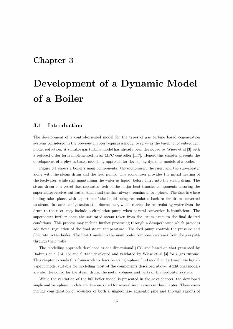
Chapter 3
Development of a Dynamic Model
of a Boiler
3.1 Introduction
The development of a control-oriented model for the types of gas turbine based cogeneration
systems considered in the previous chapter requires a model to serve as the baseline for subsequent
model reduction. A suitable gas turbine model has already been developed by Wiese et al [3] with
a reduced order form implemented in an MPC controller [117]. Hence, this chapter presents the
development of a physics-based modelling approach for developing dynamic models of a boiler.
Figure 3.1 shows a boiler’s main components: the economiser, the riser, and the superheater
along with the steam drum and the feed pump. The economiser provides the initial heating of
the feedwater, while still maintaining the water as liquid, before entry into the steam drum. The
steam drum is a vessel that separates each of the major heat transfer components ensuring the
superheater receives saturated steam and the riser always remains as two phase. The riser is where
boiling takes place, with a portion of the liquid being recirculated back to the drum converted
to steam. In some configurations the downcomer, which carries the recirculating water from the
drum to the riser, may include a circulation pump when natural convection is insufficient. The
superheater further heats the saturated steam taken from the steam drum to the final desired
conditions. This process may include further processing through a desuperheater which provides
additional regulation of the final steam temperature. The feed pump controls the pressure and
flow rate to the boiler. The heat transfer to the main boiler components comes from the gas path
through their walls.
The modelling approach developed is one dimensional (1D) and based on that presented by
Badmus et al [14, 15] and further developed and validated by Wiese et al [3] for a gas turbine.
This chapter extends this framework to describe a single-phase fluid model and a two-phase liquid-
vapour model suitable for modelling most of the components described above. Additional models
are also developed for the steam drum, the metal volumes and parts of the feedwater system.
While the validation of the full boiler model is presented in the next chapter, the developed
single and two-phase models are demonstrated for several simple cases in this chapter. These cases
include consideration of acoustics of both a single-phase adiabatic pipe and through regions of
37
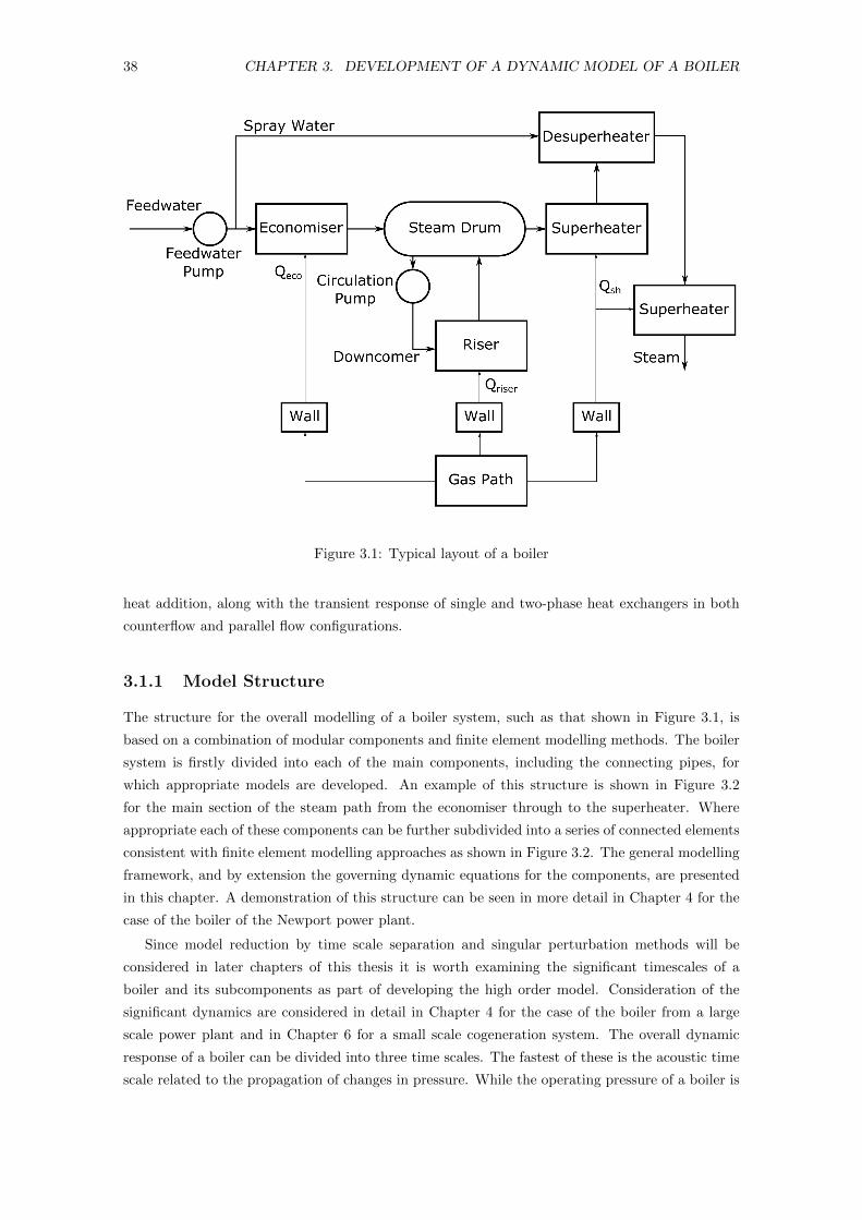
38 CHAPTER 3. DEVELOPMENT OF A DYNAMIC MODEL OF A BOILER
Figure 3.1: Typical layout of a boiler
heat addition, along with the transient response of single and two-phase heat exchangers in both
counterflow and parallel flow configurations.
3.1.1 Model Structure
The structure for the overall modelling of a boiler system, such as that shown in Figure 3.1, is
based on a combination of modular components and finite element modelling methods. The boiler
system is firstly divided into each of the main components, including the connecting pipes, for
which appropriate models are developed. An example of this structure is shown in Figure 3.2
for the main section of the steam path from the economiser through to the superheater. Where
appropriate each of these components can be further subdivided into a series of connected elements
consistent with finite element modelling approaches as shown in Figure 3.2. The general modelling
framework, and by extension the governing dynamic equations for the components, are presented
in this chapter. A demonstration of this structure can be seen in more detail in Chapter 4 for the
case of the boiler of the Newport power plant.
Since model reduction by time scale separation and singular perturbation methods will be
considered in later chapters of this thesis it is worth examining the significant timescales of a
boiler and its subcomponents as part of developing the high order model. Consideration of the
significant dynamics are considered in detail in Chapter 4 for the case of the boiler from a large
scale power plant and in Chapter 6 for a small scale cogeneration system. The overall dynamic
response of a boiler can be divided into three time scales. The fastest of these is the acoustic time
scale related to the propagation of changes in pressure. While the operating pressure of a boiler is
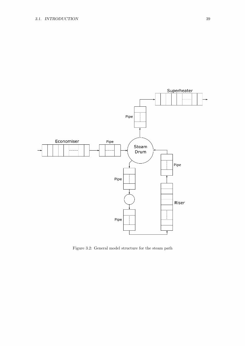
3.1. INTRODUCTION 39
Figure 3.2: General model structure for the steam path
40 CHAPTER 3. DEVELOPMENT OF A DYNAMIC MODEL OF A BOILER
of significant importance, as demonstrated by the boiler models considered in Chapter 2, this time
scale is not very significant with regards to the actual operation of the boiler. The second time
scale is the convective time scale associated with propagation of changes with the fluid flow. While
the convective time scale typically has significance in terms of the filling and emptying of volumes
in the boiler it is not the dominant time scale. The most significant time scale in the operation
of a boiler is related to the thermal inertia of the metal volumes. The dynamics of the metal
volumes are the slowest and, since these metal volumes are critical to the heat transfer between
the gas and steam paths, dominates the dynamic response of the boiler. Furthermore, maintaining
the structural integrity of the boiler is primarily governed by controlling the dynamic response of
the temperatures of these metal volumes. As will be demonstrated in Chapter 4 for the Newport
power plant the time scales of the imposed transients are typically comparable to the time scales
of the metal volumes. Nevertheless, to fully describe the system, and provide a suitable high order
model, all of these time scales need to be considered. Furthermore, as will be demonstrated in
Chapter 6 additional time scales need to be considered when the boiler is part of a larger system,
such as those of the shaft dynamics in a gas turbine based cogeneration system.
3.1.2 Modelling Framework
The modelling framework presented in this chapter is based on the framework developed by Badmus
et al [14, 15] for the case of a callorically perfect gas. As established in Chapter 2 this framework
is well structured for model reduction by time scale separation and singular perturbation methods.
Furthermore, this framework permits the dynamics of the model to be defined based of the steady
behaviour of the system. Hence, the model can be defined in the absence of potentially difficult
dynamics studies of the system. The modelling framework developed by Badmus et al [14, 15], is
based on the general one dimensional conservation equations as given by
∂
∂t(ρA) +
∂
∂y(ρuA) = 0, (3.1)
∂
∂t(ρuA) +
∂
∂y
[(ρu2 + Ps
)A]
= Ps∂A
∂y+ ρA (fs + fw) , (3.2)
∂
∂t
[ρ
(e+
u2
2
)A
]+
∂
∂y
[ρuA
(e+
Psρ
+u2
2
)]= AQ+ ρuAfs, (3.3)
where the source terms Q, fs, and fw represent the effects of heat transfer, body forces, and
friction respectively. While the model developed by Badmus et al [14, 15] and further developed
by Wiese et al [3] specifically considered an ideal gas system with constant specific heat the basic
concept of the framework is generally applicable to any system, requiring only the derivation of
appropriate influence coefficients and forcing terms. Following a similar process as Badmus et al
[14, 15], the modelling framework for the single and two-phase fluid models can therefore be defined
by recasting these equations into a discretised set of equations in matrix form,
d
dt
ρout
Ps,out
uin
= − G
∆y
ρout − ρin −m1
Ps,out − Ps,in −m2
uout − uin −m3
, (3.4)
with the matrix of influence coefficients G, and forcing terms mi, determined in Sections 3.2 and
3.3 for the single and two-phase models respectively. The forcing terms can be determined from
3.2. SINGLE-PHASE FLUID MODEL 41
the steady state behaviour of the relevant component which as stated permits dynamic studies of
the system to be avoided.
Equation (3.4) shows that the chosen state variables of the system are the density ρ, pressure
Ps, and the velocity u. These were chosen as they offered variables with recognisable physical
meaning and offered consistency between single and two-phase fluids, as well as remaining as
consistent as possible with the original framework developed by Badmus et al [14, 15]. In particular
density is convenient for the two-phase model as it can be related to the void fraction, which is
described later in Section 3.3, and the saturation values which can themselves be defined in terms
of pressure. Furthermore, pressure is itself an important variable in boiler operation. While the
original framework included the Mach number, this is not practical for a two-phase fluid considering
the difficult nature of calculating the speed of sound. Velocity was a suitable alternative that
remained consistent between the single and two-phase models and provided a variable associated
with fluid movement.
This modelling approach describes the dynamics of the main single and two-phase fluid elements
associated with the economiser, superheater, riser, desuperheater, and gas path shown in Figure
3.1. Additional fluid models not based on this framework are developed for the steam drum,
feedwater system, and the circulation pump along with a dynamic model for the metal volumes
that form the walls linking the heat transfer between relevant fluid components as shown in Figure
3.1.
This modelling framework allows for a modular approach, as established in Section 3.1.1, en-
abling a variety of boiler systems to be modelled. Furthermore, with the forcing terms constructed
from steady state behaviour and the influence coefficients derived from the general conservation
equations (3.1), (3.2), and (3.3), the model can be completely defined in the absence of transient
information, significantly simplifying model development.
Sections 3.2 and 3.3 present the derivation process for converting (3.1), (3.2), and (3.3) into
the form of (3.4) for the single and two-phase models respectively. These sections further include
the calculation processes for obtaining the forcing terms for component types relevant to the single
and two-phase models.
3.2 Single-Phase Fluid Model
The single-phase fluid model extends the modelling approach of Badmus et al [14, 15] and Wiese et
al [3]. This extended model describes the behaviour of components of the economiser, superheater,
gas path and parts of the feedwater system or any single-phase fluid component subject to the
following assumptions:
• the cross-sectional area may vary spatially;
• the fluid may be a mixture;
• the fluid equation of state is known;
• the fluid is single phase at all times;
• a single-phase component consists of a single fluid inlet and a single fluid outlet.
The development of this model requires the conversion of (3.1), (3.2), and (3.3) to the framework
of (3.4) for the case of a single-phase fluid. Expanding and recasting these equations in terms of
the density, pressure and velocity leads to the following governing set of differential equations
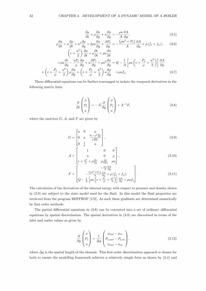
42 CHAPTER 3. DEVELOPMENT OF A DYNAMIC MODEL OF A BOILER
∂ρ
∂t+ ρ
∂u
∂y+ u
∂ρ
∂y= −ρu
A
∂A
∂y, (3.5)
ρ∂u
∂t+ u
∂ρ
∂t+ u2 ∂ρ
∂y+ 2ρu
∂u
∂y+∂Ps∂y
= −(ρu2 + Ps
)A
∂A
∂y+ ρ (fs + fw) , (3.6)(
e+u2
2
)∂ρ
∂t+ ρ
∂e
∂t+ ρu
∂u
∂t
+ρu∂e
∂y− uPs
ρ
∂ρ
∂y+ u
∂Ps∂y
+ ρu2 ∂u
∂y= Q− 1
A
[ρu
(e+
Psρ
+u2
2
)]∂A
∂y
+
(e+
Psρ
+u2
2
)ρ∂u
∂y+
(e+
Psρ
+u2
2
)u∂ρ
∂y+ρufs. (3.7)
These differential equations can be further rearranged to isolate the temporal derivatives in the
following matrix form
∂
∂t
ρ
Ps
u
= − G∂
∂y
ρ
Ps
u
+A−1F, (3.8)
where the matrices G, A, and F are given by
G =
u 0 ρ
0 uPs−ρ2 ∂e
∂ρ
ρ ∂e∂Ps
0 1ρ u
, (3.9)
A =
1 0 0
u 0 ρ
e+ u2
2 + ρ ∂e∂ρ ρ ∂e∂Ps
ρu
, (3.10)
F =
−ρuA
∂A∂y
− (ρu2+Ps)A
∂A∂y + ρ (fs + fw)
Q− 1A
[ρu(e+ Ps
ρ + u2
2
)]∂A∂y + ρufs
. (3.11)
The calculation of the derivatives of the internal energy with respect to pressure and density shown
in (3.9) are subject to the state model used for the fluid. In this model the fluid properties are
retrieved from the program REFPROP [172]. As such these gradients are determined numerically
by first order methods.
The partial differential equations in (3.8) can be converted into a set of ordinary differential
equations by spatial discretisation. The spatial derivatives in (3.8) are discretised in terms of the
inlet and outlet values as given by
∂
∂y
ρ
Ps
u
=1
∆y
ρout − ρin
Ps,out − Ps,inuout − uin
, (3.12)
where ∆y is the spatial length of the element. This first order discretisation approach is chosen for
both to ensure the modelling framework achieves a relatively simple form as shown by (3.4) and
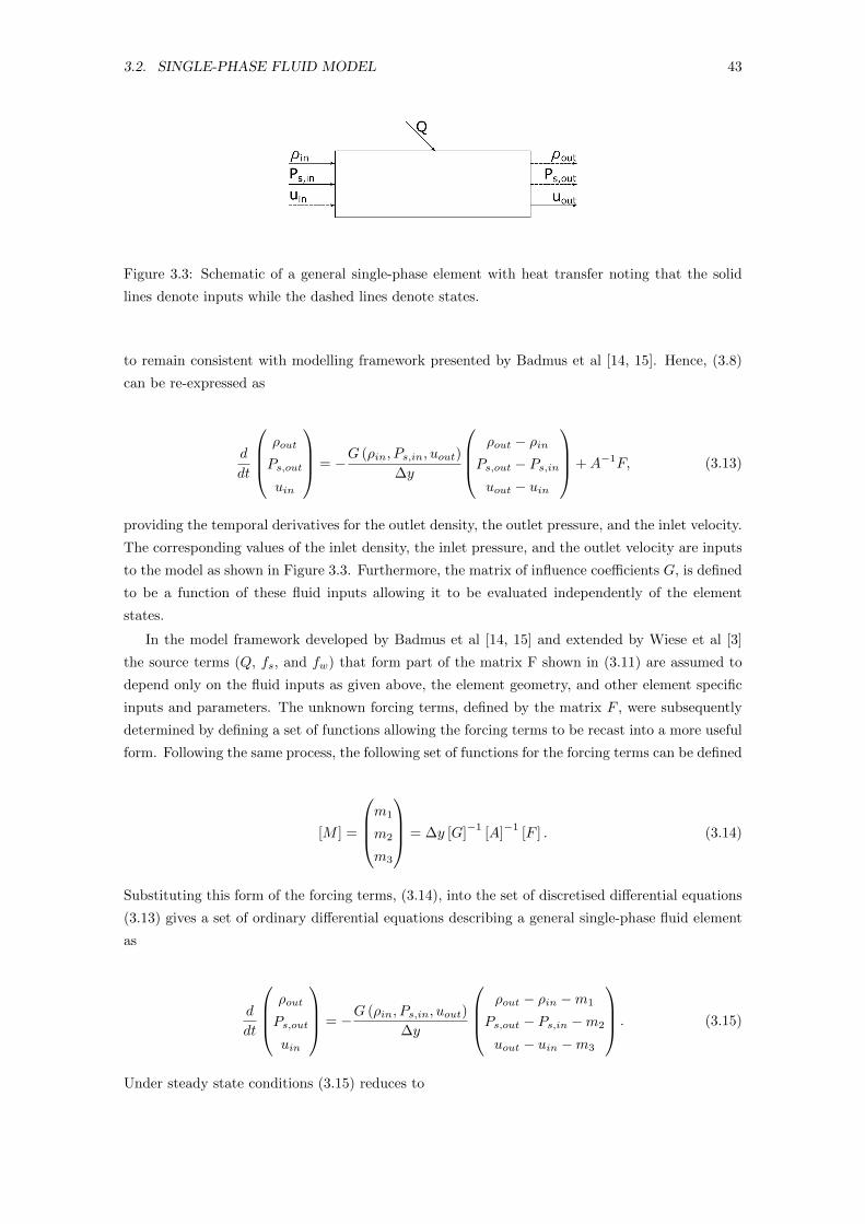
3.2. SINGLE-PHASE FLUID MODEL 43
Figure 3.3: Schematic of a general single-phase element with heat transfer noting that the solid
lines denote inputs while the dashed lines denote states.
to remain consistent with modelling framework presented by Badmus et al [14, 15]. Hence, (3.8)
can be re-expressed as
d
dt
ρout
Ps,out
uin
= −G (ρin, Ps,in, uout)
∆y
ρout − ρin
Ps,out − Ps,inuout − uin
+A−1F, (3.13)
providing the temporal derivatives for the outlet density, the outlet pressure, and the inlet velocity.
The corresponding values of the inlet density, the inlet pressure, and the outlet velocity are inputs
to the model as shown in Figure 3.3. Furthermore, the matrix of influence coefficients G, is defined
to be a function of these fluid inputs allowing it to be evaluated independently of the element
states.
In the model framework developed by Badmus et al [14, 15] and extended by Wiese et al [3]
the source terms (Q, fs, and fw) that form part of the matrix F shown in (3.11) are assumed to
depend only on the fluid inputs as given above, the element geometry, and other element specific
inputs and parameters. The unknown forcing terms, defined by the matrix F , were subsequently
determined by defining a set of functions allowing the forcing terms to be recast into a more useful
form. Following the same process, the following set of functions for the forcing terms can be defined
[M ] =
m1
m2
m3
= ∆y [G]−1
[A]−1
[F ] . (3.14)
Substituting this form of the forcing terms, (3.14), into the set of discretised differential equations
(3.13) gives a set of ordinary differential equations describing a general single-phase fluid element
as
d
dt
ρout
Ps,out
uin
= −G (ρin, Ps,in, uout)
∆y
ρout − ρin −m1
Ps,out − Ps,in −m2
uout − uin −m3
. (3.15)
Under steady state conditions (3.15) reduces to
44 CHAPTER 3. DEVELOPMENT OF A DYNAMIC MODEL OF A BOILER
m1
m2
m3
=
ρout − ρin
Ps,out − Ps,inuout − uin
, (3.16)
providing a set of equations the forcing term mapping functions, m1, m2, and m3, are required
to satisfy. Hence, these forcing term maps can be derived from the steady state behaviour of the
relevant element.
For the boiler components described by the single-phase fluid model the main element types
being considered are:
• an adiabatic pipe of uniform cross-sectional area;
• a component of uniform cross-sectional area with heat transfer;
• adiabatic components with spatial cross sectional area change.
An additional heat transfer case with defined pressure loss is also considered. The calculation
of these forcing term maps is covered in the next section while the derivations can be found in
Appendix A.
In addition to the general single-phase model, several additional special cases are considered
separately including models for the desuperheater, circulation pump, and furnace. These cases,
while still single phase, incorporate either significant deviations from the general model or in the
case of the furnace require additional considerations.
3.2.1 Single-Phase Forcing Term Map Derivation
3.2.1.1 Adiabatic Pipe of Uniform Cross-Sectional Area
The pipe elements of a boiler can reasonably be treated as components of uniform cross sectional
area with negligible heat transfer or pressure losses. Hence, under conservation of mass, momentum,
and energy at steady state, the forcing terms are small and the map functions are
m1 = 0, (3.17)
m2 = 0, (3.18)
m3 = 0. (3.19)
3.2.1.2 Component of Uniform Cross-Sectional Area With Heat Transfer
The single-phase heat transfer components of a boiler, namely the economiser and superheater, are
most commonly constructed from tube bundles of uniform geometry in either a water or fire tube
configuration, although the water tube arrangement is more common. Since the corresponding shell
is also typically of uniform geometry, these components can be described by elements of uniform
cross sectional area. At steady state, the conservation of mass, momentum and energy equations
for a single-phase fluid subject to heat transfer can be expressed as
3.2. SINGLE-PHASE FLUID MODEL 45
min = mout, (3.20)
minuin + Ps,inAcr,in = moutuout + Ps,outAcr,out, (3.21)
min
(hin +
u2in
2
)+Q = mout
(hout +
u2out
2
). (3.22)
The net heat transfer Q, is the heat transfer between the fluid and all relevant wall elements. The
number of associated wall elements for a given fluid element is dependent on the configuration of
the boiler. Economiser or superheater elements typically only have one wall element while those
of the gas path may have multiple elements. The heat transfer is defined to be a function of the
fluid temperature Ts,fluid, and the wall temperature Tw,
Q = f (Ts,fluid, Tw) . (3.23)
The heat transfer calculation is covered separately in Section 3.4. However, a suitable rep-
resentative fluid temperature is required and is defined to be the average of the inlet and outlet
temperatures of an element,
Ts,fluid =Ts,in + Ts,out
2, (3.24)
noting that Ts,out is determined from the map function steady state values and not the current state.
To determine the map functions for the forcing terms, the governing steady state equations (3.20),
(3.21), and (3.22) need to be solved for the state values (ρout, Ps,out, uin) defined earlier. Note
that the wall temperature is also treated as an input, while the representative fluid temperature
is a function of the inputs to the element via the equation of state.
Conservation of mass and momentum can be re-expressed to obtain functions for uin and Ps,out
in terms of ρout as follows
uin =ρoutuoutρin
, (3.25)
Ps,out =(ρinu
2in + Ps,in
)− ρoutu2
out. (3.26)
Combining (3.25) and (3.26) with conservation of energy, as given by (3.22), allows for ρout to be
solved for iteratively. The forcing term map function values can then be determined from (3.16).
3.2.1.3 Component of Uniform Cross-Sectional Area With Heat Transfer and Pres-
sure Loss
In practice real pipes experience pressure losses related to frictional losses and changes in pipe
geometry. In general empirical relations can be used to estimate the major losses associated with
friction and the additional minor losses. However, where suitable pressure data is available it
is simpler to determine the pressure loss for the component directly. Since, existing correlations
(see [173]) are approximately proportional to the square of the velocity the fluid the pressure loss
through a component can be defined as
46 CHAPTER 3. DEVELOPMENT OF A DYNAMIC MODEL OF A BOILER
∆Ps = βi(αpu
2out + C
)(3.27)
where βi is a scaling factor, αp is a fitted parameter, and C is a constant term accounting for
any pressure losses independent of the velocity. The fitted parameter, αp, is determined from the
available pressure data of the plant being considered. Similarly, the constant C can be determined
from pressure data. The scaling factor, βi, is used where the pressure loss is fitted over a sequence
of components and represents the proportion each component contributes to the pressure loss.
Since the pressure losses in a boiler will increase with length, the scaling factor can be defined as
a given elements fraction of the total length of a sequence of elements,
βi =Li
Ltotal. (3.28)
Hence, the outlet pressure of a component can be defined as
Ps,out = Ps,in −(βi(αpu
2out + C
))(3.29)
The forcing term map function values of this component type are evaluated in the same manner
as the previous case, with the pressure relation (3.29) replacing the rearranged conservation of
momentum expression given by (3.26). The process is otherwise the same with the forcing terms
determined iteratively to satisfy conservation of mass and energy given by (3.20) and (3.22).
This approach provides a simpler method to determine the forcing term map functions when
pressure data is available for the system. When this data is not available conventional empirical
methods will be required instead of (3.29).
3.2.1.4 Adiabatic Components With Spatial Cross-Sectional Area Change
While individual components may have uniform cross-sectional area, changes in tube diameter are
required in some places. Examples include the small header tanks that separate most components.
Since these regions of area change typically observe considerably less heat transfer than the main
heat transfer sections they can reasonably be approximated as adiabatic. Furthermore, gradual
area changes and sudden contractions can reasonably be treated as isentropic [13]. While sudden
expansions are typically non-isentropic and incur total pressure losses, it is assumed in this model
that the losses are sufficiently small enough for the component to be treated as approximately
isentropic. This permits the simpler isentropic approach presented here to be used for all elements
of cross-sectional area change. While this may introduce a small degree of error it is expected that
for the type of boiler system being considered, which is ultimately dominated by the heat transfer
components, this error should be small. With conservation of mass given by (3.20) the remaining
governing steady state equations, conservation of energy and entropy, are given by
Sin = Sout (3.30)
min
(hin +
u2in
2
)= mout
(hout +
u2out
2
)(3.31)
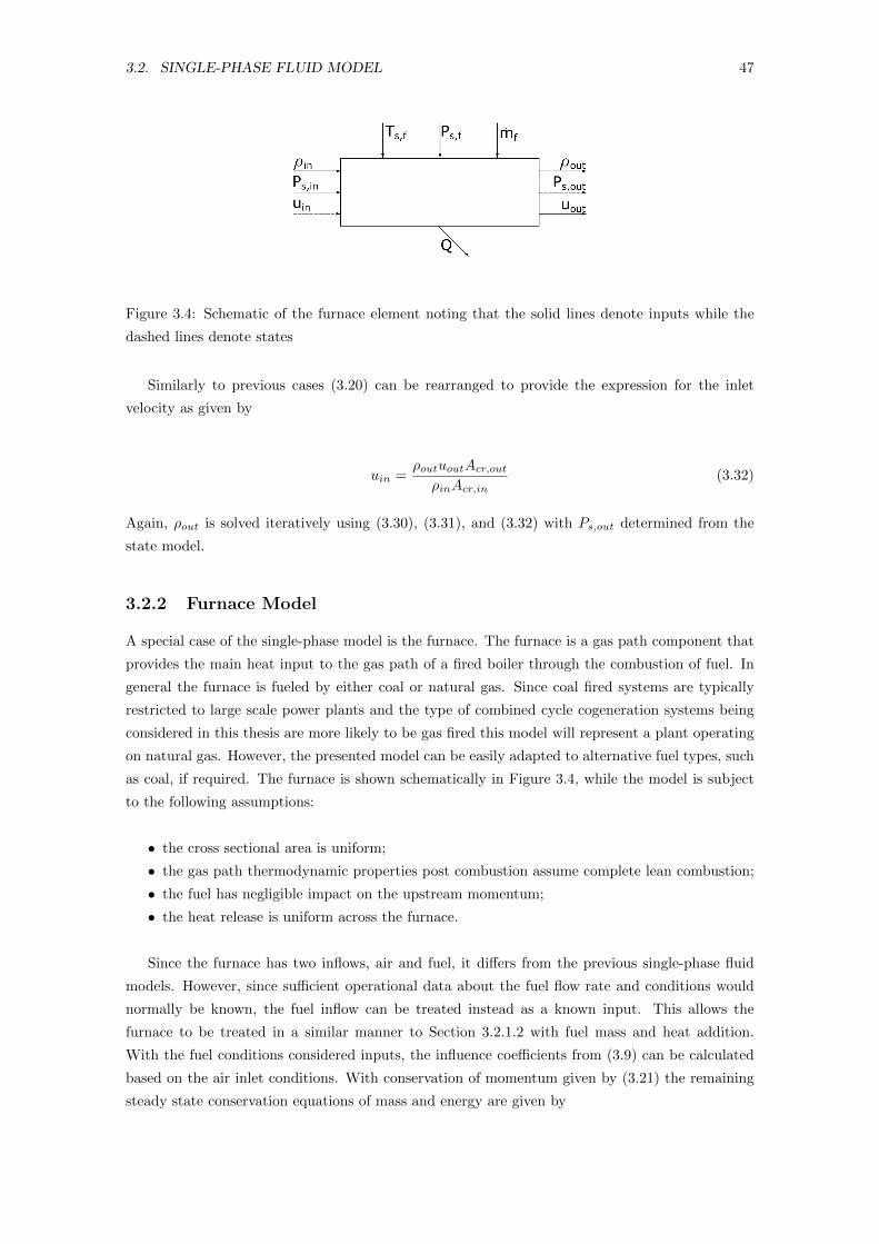
3.2. SINGLE-PHASE FLUID MODEL 47
Figure 3.4: Schematic of the furnace element noting that the solid lines denote inputs while the
dashed lines denote states
Similarly to previous cases (3.20) can be rearranged to provide the expression for the inlet
velocity as given by
uin =ρoutuoutAcr,outρinAcr,in
(3.32)
Again, ρout is solved iteratively using (3.30), (3.31), and (3.32) with Ps,out determined from the
state model.
3.2.2 Furnace Model
A special case of the single-phase model is the furnace. The furnace is a gas path component that
provides the main heat input to the gas path of a fired boiler through the combustion of fuel. In
general the furnace is fueled by either coal or natural gas. Since coal fired systems are typically
restricted to large scale power plants and the type of combined cycle cogeneration systems being
considered in this thesis are more likely to be gas fired this model will represent a plant operating
on natural gas. However, the presented model can be easily adapted to alternative fuel types, such
as coal, if required. The furnace is shown schematically in Figure 3.4, while the model is subject
to the following assumptions:
• the cross sectional area is uniform;
• the gas path thermodynamic properties post combustion assume complete lean combustion;
• the fuel has negligible impact on the upstream momentum;
• the heat release is uniform across the furnace.
Since the furnace has two inflows, air and fuel, it differs from the previous single-phase fluid
models. However, since sufficient operational data about the fuel flow rate and conditions would
normally be known, the fuel inflow can be treated instead as a known input. This allows the
furnace to be treated in a similar manner to Section 3.2.1.2 with fuel mass and heat addition.
With the fuel conditions considered inputs, the influence coefficients from (3.9) can be calculated
based on the air inlet conditions. With conservation of momentum given by (3.21) the remaining
steady state conservation equations of mass and energy are given by
48 CHAPTER 3. DEVELOPMENT OF A DYNAMIC MODEL OF A BOILER
min + mf = mout, (3.33)
min
(hin +
u2in
2
)+ mf
(hf +
u2f
2
)+Q+Qf = mout
(hout +
u2out
2
). (3.34)
The heat release from the fuel is calculated from the lower calorific value of the fuel as
Qf = mfLCVf (3.35)
The heat transfer Q, however, requires a different approach to the previous heat transfer com-
ponents as the influence of fuel heat release and the strong effect of radiation causes the average
of inlet and outlet temperatures to be unsuitable as a representative temperature. This is resolved
by dividing the furnace into a series of smaller subelements for which this average temperature is
a suitable representative of the fluid temperature. To simplify this process it is further assumed
that for these subelements that they can be treated as a calorically perfect gas. Hence, for a
given subelement the outlet temperature Ts,el,out, can be defined as a function of the element inlet
temperature, Ts,el,in and the flow rate as
Ts,el,out = Ts,el,in +(Qf,el +Qel)
mCp, (3.36)
where Qf,el is the heat release from the fuel for a given subelement and Qel is the heat transfer for
a given subelement calculated as per Section 3.4. The net furnace heat transfer can subsequently
be determined as the summation of the heat transfers for each subelement, with a representative
fluid temperature not required. Hence, the furnace heat transfer can be determined as a function of
the mass flow rate. Similarly to the previous cases (3.33), (3.21), and (3.34) are solved iteratively
with the forcing terms determined as per previous cases.
It is also necessary to consider the composition of the gas path after combustion. It will be
assumed that methane is sufficiently representative of the fuel. Assuming a lean mixture and
complete combustion dictates that
CH4 + a (O2 + 3.76N2)→ 2H2O + CO2 + bO2 + 3.76aN2, (3.37)
where the stoichiometric coefficients of air and excess oxygen in the products are given by
a = AFR
(MC + 4MH
2MO + 7.52MN
), (3.38)
b = a− 2. (3.39)
The mole fractions of the products are
yH2O =2
1 + 4.76a, (3.40)
yCO2=
1
1 + 4.76a, (3.41)
yO2=
a− 2
1 + 4.76a, (3.42)
yN2=
3.76a
1 + 4.76a, (3.43)
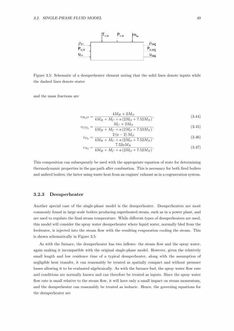
3.2. SINGLE-PHASE FLUID MODEL 49
Figure 3.5: Schematic of a desuperheater element noting that the solid lines denote inputs while
the dashed lines denote states
and the mass fractions are
cH2O =4MH + 2MO
4MH +MC + a (2MO + 7.52MN ), (3.44)
cCO2=
MC + 2MO
4MH +MC + a (2MO + 7.52MN ), (3.45)
cO2 =2 (a− 2)MO
4MH +MC + a (2MO + 7.52MN ), (3.46)
cN2=
7.52aMN
4MH +MC + a (2MO + 7.52MN ). (3.47)
This composition can subsequently be used with the appropriate equation of state for determining
thermodynamic properties in the gas path after combustion. This is necessary for both fired boilers
and unfired boilers, the latter using waste heat from an engines’ exhaust as in a cogeneration system.
3.2.3 Desuperheater
Another special case of the single-phase model is the desuperheater. Desuperheaters are most
commonly found in large scale boilers producing superheated steam, such as in a power plant, and
are used to regulate the final steam temperature. While different types of desuperheaters are used,
this model will consider the spray water desuperheater where liquid water, normally bled from the
feedwater, is injected into the steam flow with the resulting evaporation cooling the steam. This
is shown schematically in Figure 3.5.
As with the furnace, the desuperheater has two inflows: the steam flow and the spray water,
again making it incompatible with the original single-phase model. However, given the relatively
small length and low residence time of a typical desuperheater, along with the assumption of
negligible heat transfer, it can reasonably be treated as spatially compact and without pressure
losses allowing it to be evaluated algebraically. As with the furnace fuel, the spray water flow rate
and conditions are normally known and can therefore be treated as inputs. Since the spray water
flow rate is small relative to the steam flow, it will have only a small impact on steam momentum,
and the desuperheater can reasonably be treated as isobaric. Hence, the governing equations for
the desuperheater are
50 CHAPTER 3. DEVELOPMENT OF A DYNAMIC MODEL OF A BOILER
min + mw = mout, (3.48)
Ps,in = Ps,out, (3.49)
Ht,in +Ht,w = Ht,out. (3.50)
Since the desuperheater is treated as algebraic, equations (3.48), (3.49), and (3.50) can be used to
determine the output states of the desuperheater as shown in Figure 3.5.
3.2.4 Circulation Pump
The circulation pump is normally used in forced circulation boilers to increase the circulation rate
over that which would be achieved by natural circulation. This is usually required for systems
where the difference in vapour and liquid density in the risers is insufficient to drive the required
circulation rate. In this study the circulation pump is treated as a special case where there
is insufficient information to adequately describe the dynamic behaviour of the pump. Where
sufficient information is present the feedwater pump model described in section 3.8.1 may be used.
The circulation pump, if required, generally only provides a small pressure rise relative to the
pressure through the risers. As such the pump can be modeled as a constant pressure rise with the
process assumed to be isothermal. Since the pump can be considered compact with regards to flow
length, and the pump shaft dynamics are fast, the circulation pump can be treated as algebraic.
Hence, the governing equations, along with conservation of mass given by (3.20), are given by
Ps,out = Ps,in + ∆Ps, (3.51)
Ts,out = Ts,in, (3.52)
(3.53)
where ∆Ps is the fixed pressure rise.
3.3 Two-Phase Fluid Model
The two-phase fluid model again extends the approach of Badmus et al [14, 15]. A boiling fluid
will be considered for the riser and associated two-phase components. The two-phase model is
also applicable to a condensing process or any two-phase process subject to the following model
assumptions:
• the cross-sectional area may vary spatially;
• the fluid is pure;
• the fluid is within the wet region and as such the thermodynamic properties of each phase
are the saturated values;
• the fluid equation of state is known;
• the thermodynamic properties are functions of the pressure only;
• a two-phase element consists of a single fluid inlet and a single fluid outlet.
3.3. TWO-PHASE FLUID MODEL 51
Similarly to the single-phase model, the governing one dimensional conservation equations (3.1),
(3.2), and (3.3) are adjusted to account for a two-phase fluid and subsequently converted to the
form of (3.4). The density of the fluid can be expressed in terms of the void fraction α, and the
saturation densities as
ρtp = αρg + (1− α) ρl, (3.54)
where the void fraction is the ratio of the volume of the vapour to the total volume of the fluid. In
the limit where the volume becomes infinitesimally thin, this reduces to a ratio of cross sectional
areas
α =Acr,gAcr
. (3.55)
The void fraction can be related to the dryness fraction x by
α =x
x+ SR (1− x)ρgρl
, (3.56)
where the dryness fraction is defined by
x =mg
mg +ml. (3.57)
SR is the slip ratio, which is the ratio of the velocity of the vapour phase to the velocity of the liquid
phase and is normally determined from empirical correlations [161]. Examples of such correlations
include the assumption of homogeneous flow, the Chisolm correlation, and the CISE correlation
all of which can be found in [161]. In this model, the slip ratio is defined as a function of the
fluid thermodynamic properties and the velocity, permitting any suitable slip ratio correlation to
be used. Hence, the governing equations can be derived independently of the choice of slip ratio
correlation.
A representative mass averaged velocity of the liquid and vapour velocities can be defined as
utp =m
ρtpA, (3.58)
which, along with (3.54), allows conservation of mass to be expressed in an equivalent manner
to the single-phase case. Expanding the equations for the conservation of momentum and energy
((3.2) and (3.3) respectively) to the two phases separately,
∂
∂t(ρtpA) +
∂
∂y(ρtputpA) = 0, (3.59)
∂
∂t(ρtputpA) +
∂
∂y
[(αρgu
2g + (1− α) ρlu
2l + Ps
)A]
= Ps∂A
∂y+ ρA (fs + fw) , (3.60)
∂
∂t
[(αρg
(eg +
u2g
2
)+ (1− α) ρl
(el +
u2l
2
))A
]
+∂
∂y
[(αρgug
(hg +
u2g
2
)+ (1− α) ρlul
(hl +
u2l
2
))A
]= AQ+ ρtputpAfs. (3.61)
52 CHAPTER 3. DEVELOPMENT OF A DYNAMIC MODEL OF A BOILER
The individual velocities of the liquid and vapour phases can be related to the mass averaged
velocity and the void fraction using the slip ratio,
ul =ρtputp
αρgSR+ (1− α) ρl, (3.62)
ug = SRul. (3.63)
Recasting the conservation equations (3.59), (3.60), and (3.61) in terms of the two-phase density
ρtp, the two-phase velocity utp, and the pressure Ps, leads to the following set of differential
equations describing the two-phase model
∂ρtp∂t
+ ρtp∂utp∂y
+ utp∂ρtp∂y
= −ρtputpA
∂A
∂y, (3.64)
utp∂ρtp∂t
+ ρtp∂utp∂t
+ χ1∂ρtp∂y
+ χ2∂Ps∂y
+ χ3∂utp∂y
= −χ4
A
∂A
∂y+ ρtp (fs + fw) , (3.65)
ξ1∂ρtp∂t
+ ξ2∂Ps∂t
+ ξ3∂utp∂t
+ ξ4∂ρtp∂y
+ ξ5∂Ps∂y
+ ξ6∂utp∂y
= Q− ξ7A
∂A
∂y+ ρtputpfs. (3.66)
The coefficients of the momentum equation (3.65) χi, and the energy equation (3.66) ξi are alge-
braically complex and presented in Appendix A. As per the single-phase model these terms include
derivatives of particular properties with respect to the density and pressure which are determined
numerically from first order methods.
Equations (3.64), (3.65), and (3.66) can be further rearranged in matrix form to separate the
temporal and spatial derivatives
∂
∂t
ρtp
Ps
utp
= −Gtp∂
∂y
ρtp
Ps
utp
+A−1tp Ftp, (3.67)
where the matrices Gtp, Atp, and Ftp are given by
Gtp =
utp 0 ρtp
ξ3u2tp−ρtputpξ1−χ1ξ3+ρtpξ4
ρtpξ2
ρtpξ5−χ2ξ3ρtpξ2
ρtpξ6−χ3ξ3−ρ2tpξ1+ρtputpξ3
ρtpξ2χ1−u2
tp
ρtp
χ2
ρtp
χ3−ρtputpρtp
, (3.68)
Atp =
1 0 0
utp 0 ρtp
ξ1 ξ2 ξ3
, (3.69)
Ftp =
−ρtputpA
∂A∂y
−χ4
A∂A∂y + ρtp (fs + fw)
Q− ξ7A∂A∂y + ρtputpfs
. (3.70)
Following the same process for the single-phase model, the set of partial differential equations
in (3.67) can be discretised to produce the following set of ordinary differential equations
d
dt
ρtp,out
Ps,out
utp,in
= −Gtp (ρtp,in, Ps,in, utp,out)
∆y
ρtp,out − ρtp,inPs,out − Ps,inutp,out − utp,in
+A−1tp Ftp, (3.71)
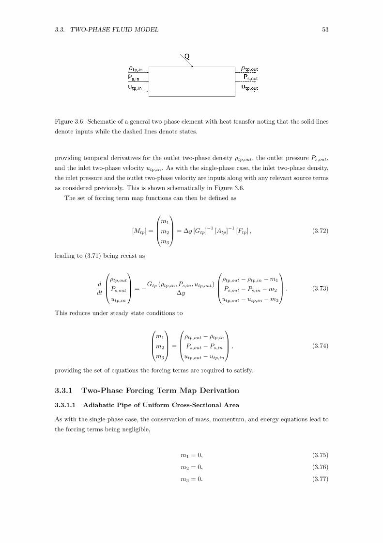
3.3. TWO-PHASE FLUID MODEL 53
Figure 3.6: Schematic of a general two-phase element with heat transfer noting that the solid lines
denote inputs while the dashed lines denote states.
providing temporal derivatives for the outlet two-phase density ρtp,out, the outlet pressure Ps,out,
and the inlet two-phase velocity utp,in. As with the single-phase case, the inlet two-phase density,
the inlet pressure and the outlet two-phase velocity are inputs along with any relevant source terms
as considered previously. This is shown schematically in Figure 3.6.
The set of forcing term map functions can then be defined as
[Mtp] =
m1
m2
m3
= ∆y [Gtp]−1
[Atp]−1
[Ftp] , (3.72)
leading to (3.71) being recast as
d
dt
ρtp,out
Ps,out
utp,in
= −Gtp (ρtp,in, Ps,in, utp,out)
∆y
ρtp,out − ρtp,in −m1
Ps,out − Ps,in −m2
utp,out − utp,in −m3
. (3.73)
This reduces under steady state conditions to
m1
m2
m3
=
ρtp,out − ρtp,inPs,out − Ps,inutp,out − utp,in
, (3.74)
providing the set of equations the forcing terms are required to satisfy.
3.3.1 Two-Phase Forcing Term Map Derivation
3.3.1.1 Adiabatic Pipe of Uniform Cross-Sectional Area
As with the single-phase case, the conservation of mass, momentum, and energy equations lead to
the forcing terms being negligible,
m1 = 0, (3.75)
m2 = 0, (3.76)
m3 = 0. (3.77)
54 CHAPTER 3. DEVELOPMENT OF A DYNAMIC MODEL OF A BOILER
3.3.1.2 Component of Uniform Cross Sectional Area With Heat Transfer
Steady state conservation of mass, momentum, and energy for a two-phase boiling or condensing
fluid are given by
mtp,in = mtp,out, (3.78)
mtpin(xinug,in + (1− xin)ul,in) + Ps,inAcr,in
= mtp,out (xoutug,out + (1− xout)ul,out) + Ps,outAcr,out, (3.79)
mtp,in
(xin
(hg,in +
u2g,in
2
)+ (1− xin)
(hl,in +
u2l,in
2
))+Q
= mtp,out
(xout
(hg,out +
u2g,out
2
)+ (1− xout)
(hl,out +
u2l,out
2
)). (3.80)
Assuming a water tube configuration, the heat transfer Q, for a riser element will normally
only be associated with a single wall element in a one-dimensional model. This heat transfer is
calculated as described in Section 3.4 and can be defined as a function of the wall temperature
Tw and a representative fluid temperature Ts,fluid, equivalent to that given by (3.23) for the
single-phase case. As with the single-phase case, the representative fluid temperature is calculated
as the average of the inlet and outlet temperatures as given by (3.24) noting that these are the
saturation temperatures for the two phase case. As before the outlet temperature Ts,out in (3.24) is
determined from the map function steady state values and not the current states. Additionally, the
wall temperature is considered an input. Furthermore, the expected high heat transfer coefficient,
as a result of the boiling process, and the resulting low temperature difference between the fluid
and the wall, allows the radiative component of heat transfer to be neglected.
Recalling that the individual phase velocities ug and ul are defined by (3.63) and (3.62) respec-
tively, and the definition of the two-phase density as given by (3.54), the steady state equations
(3.78), (3.79), (3.80) can be solved to obtain the state values (ρtp,out, Ps,out, and utp,in). However,
since the state model is treated as a black box and the slip ratio kept general to allow for the
use of different correlations, analytical representations are not available. Hence, the steady state
equations need to be solved iteratively. The forcing term maps can subsequently be calculated
from (3.74).
3.3.1.3 Adiabatic Component With Spatial Cross-Sectional Area Change
Similar to the single-phase case, the two-phase components are subject to changes in cross-sectional
area. As with the equivalent single-phase case, the short length and assumed negligible losses allow
the component to be approximated as isentropic. With conservation of mass given by (3.78), the
remaining governing steady state equations, conservation of energy and entropy, are given by
xinsg,in + (1− xin) sl,in = xoutsg,out + (1− xout) sl,out, (3.81)
xin
(hg,in +
u2g,in
2
)+ (1− xin)
(hl,in +
u2l,in
2
)= xout
(hg,out +
u2g,out
2
)
+ (1− xout)
(hl,out +
u2l,out
2
). (3.82)
3.3. TWO-PHASE FLUID MODEL 55
Recalling that the dryness fraction can be related to the state values by (3.56) and (3.54),
the above set of equations can be solved to obtain the state values (ρtp,out, Ps,out, and utp,in).
However, as with the previous case, the state model and slip ratio require these equations to be
solved iteratively. The forcing term map can then be determined from (3.74).
3.3.2 Phase Change Model
A special case of the two-phase model is that of the fluid transitioning between single phase and
two phase. Since it is common for the fluid entering the risers to still be a subcooled liquid, a
transition from single phase to two phase is required. The reverse case of a transition from two
phase to single phase does not commonly occur in the drum boiler case being considered, but would
be required for a subcritical, once through boiler. Since this latter case is not part of the model
being developed it will not be considered further. However, the principles of the phase change
model are equally applicable to this case.
Since the inlet of the element is single phase, the influence coefficients are those of the single-
phase model given by (3.9). The phase change model can otherwise be treated equivalently to the
cases of the single and two-phase models, with steady state conservation of mass, momentum, and
energy given by
min = mtp,out, (3.83)
minuin + Ps,inAcr,in = mtp,out (xoutug,out + (1− xout)ul,out) + Ps,outAcr,out, (3.84)
min
(hin +
u2in
2
)+Q = mtp,out
(xout
(hg,out +
u2g,out
2
)
+ (1− xout)
(hl,out +
u2l,out
2
)). (3.85)
As with the general two-phase heat transfer case, the heat transfer, Q, will normally only be
associated with a single wall element and calculated, as described in Section 3.4, as a function
of the representative fluid temperature and the wall temperature. Unlike the individual single
and two-phase cases, a simple average of the inlet and outlet temperatures is not a suitably rep-
resentative fluid temperature since the saturation temperature in the two-phase region will vary
significantly less than that in the single-phase region. However, where the single-phase fluid is al-
ready sufficiently close to saturation the phase change element will be dominated by the two-phase
region. Hence, a suitably representative fluid temperature is defined as the average of the outlet
temperature (which is saturated) and the saturation temperature based on the inlet pressure. As
with the cases presented previously, the temperatures used are based on the calculated steady state
values to ensure the forcing terms remain functions of the inputs only.
The steady state conservation equations (3.83), (3.84), and (3.85) can be solved similarly to
the single and two-phase heat transfer cases that have been presented previously. As with these
previous cases, it will be necessary to solve the set of equations iteratively with the forcing term
maps subsequently determined from (3.74).
56 CHAPTER 3. DEVELOPMENT OF A DYNAMIC MODEL OF A BOILER
3.4 Heat Transfer
The heat transfer between the fluid and walls is primarily governed by convection. The inclusion
of radiation is required where there is a sufficiently high temperature difference between the fluid
and the wall and, in the case of a fired boiler, there is combustion. Hence, the heat transfer can in
general be defined as
Q = Qconv (Ts,fluid, Twall) +Qrad (Ts,fluid, Twall) . (3.86)
With the exception of the furnace and phase change component types described in Sections 3.2.2
and 3.3.2 respectively, the representative fluid temperature Ts,fluid, is calculated as an average of
the inlet and outlet temperatures. Hence, the convective heat transfer term Qconv is determined
from Newton’s Law of Cooling,
Qconv = hconvAsurf (Twall − Ts,fluid) . (3.87)
Radiation can generally be neglected inside the economiser and superheater steam paths given
the dominant convective heat transfer. However, radiation can’t be neglected in the gas path given
the elevated temperatures and low convective heat transfer coefficient.
The radiative heat transfer assumes a grey gas [174],
Qrad =σAsurf εw
1− (1− εw) (1− αg)(αgT
4wall − εgT 4
s,fluid
). (3.88)
Under typical lean combustion conditions in a furnace the dominant contributions to gas radiation
come from carbon dioxide and water vapour [174]. Hence, the gas path emissivity εg, and absorp-
tivity αg are determined from empirical relationships for a CO2-H2O mixture [174]. The empirical
relationships are defined as
εg = ε (Ps, Ts,fluid, DhPs,i) , (3.89)
αg =
(TfluidTwall
)0.65
ε
(Twall, DhPs,i
TwallTs,fluid
), (3.90)
where Dh and Ps,i are the hydraulic diameter and the partial pressure of the relevant gas respec-
tively. The hydraulic diameter is given by
Dh =4AcrL
, (3.91)
where L is the wetted perimeter. The partial pressure of a particular component of the gas is
calculated from the mol fraction yi, as
Ps,i = yiPs. (3.92)
The wall emissivity, εw, can be determined using knowledge of the material and surface finish [174].
3.5. BOUNDARY CONDITION MODEL 57
3.5 Boundary Condition Model
The boundary conditions used in the model can be divided into two types:
1. Those for a fluid that can be approximated by the ideal gas law.
2. Those for a liquid or two-phase fluid.
For the first case, such as for the gas path or sufficiently superheated steam, the boundary
conditions are based on the linear one-dimensional inviscid (LODI) conditions of Poinset and Lele
[175]. A subset of these conditions are used in the inlet and outlet of the gas path and the outlet
of the steam path.
Without considering the imposed quantities and assuming negligible heat transfer, the governing
differential equations for the boundary variables in the one-dimensional case are given by
∂ρ
∂t+ d1 = 0, (3.93)
∂ρE
∂t+
1
2u2d1 +
d2
γ − 1+ ρud3 = 0, (3.94)
∂ρu
∂t+ ud1 + ρd3 = 0, (3.95)
where the energy term E is given by
E =1
2u2 +
P
γ − 1. (3.96)
The derivatives normal to the boundary di are given by
d1 =1
c2
(L2 +
1
2(L5 + L1)
), (3.97)
d2 =1
2(L5 + L1) , (3.98)
d3 =1
2ρc(L5 −L1) , (3.99)
where the amplitudes of the characteristic waves Li for internal waves are given by
L1 = λ1
(∂P
∂y− ρc∂u
∂y
), (3.100)
L2 = λ2
(c2∂ρ
∂y− ∂P
∂y
), (3.101)
L5 = λ5
(∂P
∂y+ ρc
∂u
∂y
), (3.102)
and the characteristic velocities λi are given by
λ1 = u− c, (3.103)
λ2 = u, (3.104)
λ5 = u+ c. (3.105)
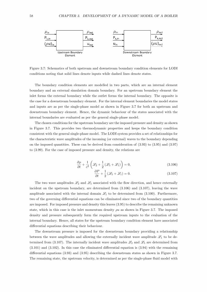
58 CHAPTER 3. DEVELOPMENT OF A DYNAMIC MODEL OF A BOILER
Figure 3.7: Schematics of both upstream and downstream boundary condition elements for LODI
conditions noting that solid lines denote inputs while dashed lines denote states.
The boundary condition elements are modelled in two parts, which are an internal element
boundary and an external simulation domain boundary. For an upstream boundary element the
inlet forms the external boundary while the outlet forms the internal boundary. The opposite is
the case for a downstream boundary element. For the internal element boundaries the model states
and inputs are as per the single-phase model as shown in Figure 3.7 for both an upstream and
downstream boundary element. Hence, the dynamic behaviour of the states associated with the
internal boundaries are evaluated as per the general single-phase model.
The chosen conditions for the upstream boundary are the imposed pressure and density as shown
in Figure 3.7. This provides two thermodynamic properties and keeps the boundary condition
consistent with the general single-phase model. The LODI system provides a set of relationships for
the characteristic wave amplitudes of the incoming (or external) waves to the boundary depending
on the imposed quantities. These can be derived from consideration of (3.93) to (3.95) and (3.97)
to (3.99). For the case of imposed pressure and density, the relations are
∂ρ
∂t+
1
c2
(L2 +
1
2(L5 + L1)
)= 0, (3.106)
∂P
∂t+
1
2(L5 + L1) = 0. (3.107)
The two wave amplitudes L2 and L5 associated with the flow direction, and hence externally
incident on the upstream boundary, are determined from (3.106) and (3.107), leaving the wave
amplitude associated with the internal domain L1 to be determined from (3.100). Furthermore,
two of the governing differential equations can be eliminated since two of the boundary quantities
are imposed. For imposed pressure and density this leaves (3.95) to describe the remaining unknown
state, which in this case is the inlet momentum density ρu as shown in Figure 3.7. The imposed
density and pressure subsequently form the required upstream inputs to the evaluation of the
internal boundary. Hence, all states for the upstream boundary condition element have associated
differential equations describing their behaviour.
The downstream pressure is imposed for the downstream boundary providing a relationship
between the wave amplitudes and allowing the externally incident wave amplitude L1 to be de-
termined from (3.107). The internally incident wave amplitudes L2 and L5 are determined from
(3.101) and (3.102). In this case the eliminated differential equation is (3.94) with the remaining
differential equations (3.93) and (3.95) describing the downstream states as shown in Figure 3.7.
The remaining state, the upstream velocity, is determined as per the single-phase fluid model with
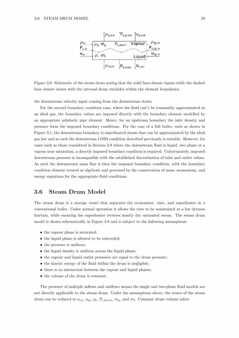
3.6. STEAM DRUM MODEL 59
Figure 3.8: Schematic of the steam drum noting that the solid lines denote inputs while the dashed
lines denote states with the internal drum variables within the element boundaries.
the downstream velocity input coming from the downstream states.
For the second boundary condition case, where the fluid can’t be reasonably approximated as
an ideal gas, the boundary values are imposed directly with the boundary element modelled by
an appropriate adiabatic pipe element. Hence, for an upstream boundary the inlet density and
pressure form the imposed boundary conditions. For the case of a full boiler, such as shown in
Figure 3.1, the downstream boundary is superheated steam that can be approximated by the ideal
gas law and as such the downstream LODI condition described previously is suitable. However, for
cases such as those considered in Section 3.9 where the downstream fluid is liquid, two phase or a
vapour near saturation, a directly imposed boundary condition is required. Unfortunately, imposed
downstream pressure is incompatible with the established discretisation of inlet and outlet values.
As such the downstream mass flux is then the imposed boundary condition, with the boundary
condition element treated as algebraic and governed by the conservation of mass, momentum, and
energy equations for the appropriate fluid conditions.
3.6 Steam Drum Model
The steam drum is a storage vessel that separates the economiser, riser, and superheater in a
conventional boiler. Under normal operation it allows the riser to be maintained at a low dryness
fraction, while ensuring the superheater receives mostly dry saturated steam. The steam drum
model is shown schematically in Figure 3.8 and is subject to the following assumptions
• the vapour phase is saturated;
• the liquid phase is allowed to be subcooled;
• the pressure is uniform;
• the liquid density is uniform across the liquid phase;
• the vapour and liquid outlet pressures are equal to the drum pressure;
• the kinetic energy of the fluid within the drum is negligible;
• there is no interaction between the vapour and liquid phases;
• the volume of the drum is constant.
The presence of multiple inflows and outflows means the single and two-phase fluid models are
not directly applicable to the steam drum. Under the assumptions above, the states of the steam
drum can be reduced to uin, utp, ρl, Ps,drum, mg, and ml. Constant drum volume infers
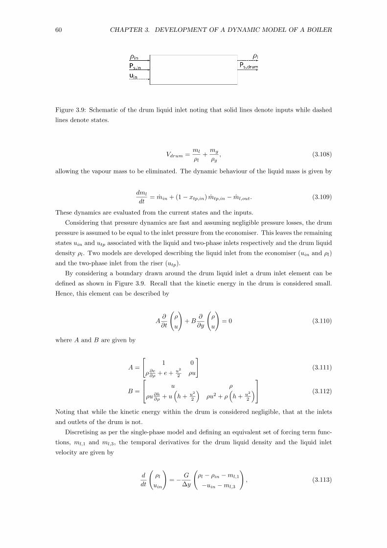
60 CHAPTER 3. DEVELOPMENT OF A DYNAMIC MODEL OF A BOILER
Figure 3.9: Schematic of the drum liquid inlet noting that solid lines denote inputs while dashed
lines denote states.
Vdrum =ml
ρl+mg
ρg, (3.108)
allowing the vapour mass to be eliminated. The dynamic behaviour of the liquid mass is given by
dml
dt= min + (1− xtp,in) mtp,in − ml,out. (3.109)
These dynamics are evaluated from the current states and the inputs.
Considering that pressure dynamics are fast and assuming negligible pressure losses, the drum
pressure is assumed to be equal to the inlet pressure from the economiser. This leaves the remaining
states uin and utp associated with the liquid and two-phase inlets respectively and the drum liquid
density ρl. Two models are developed describing the liquid inlet from the economiser (uin and ρl)
and the two-phase inlet from the riser (utp).
By considering a boundary drawn around the drum liquid inlet a drum inlet element can be
defined as shown in Figure 3.9. Recall that the kinetic energy in the drum is considered small.
Hence, this element can be described by
A∂
∂t
(ρ
u
)+B
∂
∂y
(ρ
u
)= 0 (3.110)
where A and B are given by
A =
[1 0
ρ ∂e∂ρ + e+ u2
2 ρu
](3.111)
B =
u ρ
ρu∂h∂ρ + u(h+ u2
2
)ρu2 + ρ
(h+ u2
2
) (3.112)
Noting that while the kinetic energy within the drum is considered negligible, that at the inlets
and outlets of the drum is not.
Discretising as per the single-phase model and defining an equivalent set of forcing term func-
tions, ml,1 and ml,3, the temporal derivatives for the drum liquid density and the liquid inlet
velocity are given by
d
dt
(ρl
uin
)= − G
∆y
(ρl − ρin −ml,1
−uin −ml,3
), (3.113)
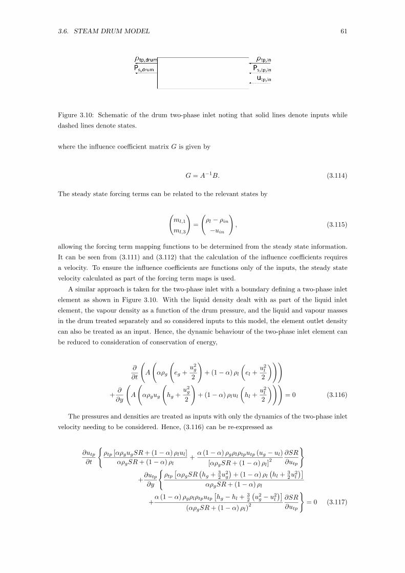
3.6. STEAM DRUM MODEL 61
Figure 3.10: Schematic of the drum two-phase inlet noting that solid lines denote inputs while
dashed lines denote states.
where the influence coefficient matrix G is given by
G = A−1B. (3.114)
The steady state forcing terms can be related to the relevant states by
(ml,1
ml,3
)=
(ρl − ρin−uin
), (3.115)
allowing the forcing term mapping functions to be determined from the steady state information.
It can be seen from (3.111) and (3.112) that the calculation of the influence coefficients requires
a velocity. To ensure the influence coefficients are functions only of the inputs, the steady state
velocity calculated as part of the forcing term maps is used.
A similar approach is taken for the two-phase inlet with a boundary defining a two-phase inlet
element as shown in Figure 3.10. With the liquid density dealt with as part of the liquid inlet
element, the vapour density as a function of the drum pressure, and the liquid and vapour masses
in the drum treated separately and so considered inputs to this model, the element outlet density
can also be treated as an input. Hence, the dynamic behaviour of the two-phase inlet element can
be reduced to consideration of conservation of energy,
∂
∂t
(A
(αρg
(eg +
u2g
2
)+ (1− α) ρl
(el +
u2l
2
)))
+∂
∂y
(A
(αρgug
(hg +
u2g
2
)+ (1− α) ρlul
(hl +
u2l
2
)))= 0 (3.116)
The pressures and densities are treated as inputs with only the dynamics of the two-phase inlet
velocity needing to be considered. Hence, (3.116) can be re-expressed as
∂utp∂t
{ρtp [αρgugSR+ (1− α) ρlul]
αρgSR+ (1− α) ρl+α (1− α) ρgρlρtputp (ug − ul)
[αρgSR+ (1− α) ρl]2
∂SR
∂utp
}
+∂utp∂y
{ρtp[αρgSR
(hg + 3
2u2g
)+ (1− α) ρl
(hl + 3
2u2l
)]αρgSR+ (1− α) ρl
+α (1− α) ρgρlρtputp
[hg − hl + 3
2
(u2g − u2
l
)](αρgSR+ (1− α) ρl)
2
∂SR
∂utp
}= 0 (3.117)
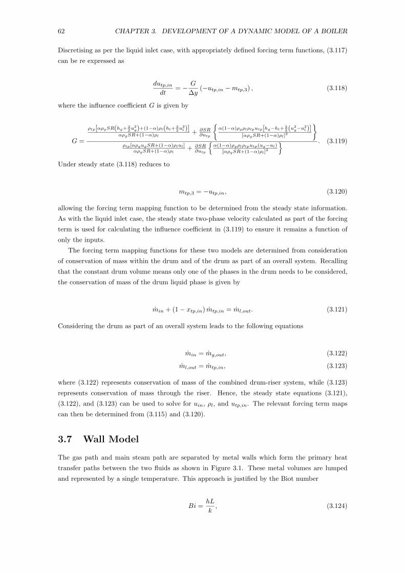
62 CHAPTER 3. DEVELOPMENT OF A DYNAMIC MODEL OF A BOILER
Discretising as per the liquid inlet case, with appropriately defined forcing term functions, (3.117)
can be re expressed as
dutp,indt
= − G
∆y(−utp,in −mtp,3) , (3.118)
where the influence coefficient G is given by
G =
ρtp[αρgSR(hg+ 32u
2g)+(1−α)ρl(hl+ 3
2u2l )]
αρgSR+(1−α)ρl+ ∂SR
∂utp
{α(1−α)ρgρlρtputp[hg−hl+ 3
2 (u2g−u
2l )]
[αρgSR+(1−α)ρl]2
}ρtp[αρgugSR+(1−α)ρlul]
αρgSR+(1−α)ρl+ ∂SR
∂utp
{α(1−α)ρgρlρtputp(ug−ul)
[αρgSR+(1−α)ρl]2
} . (3.119)
Under steady state (3.118) reduces to
mtp,3 = −utp,in, (3.120)
allowing the forcing term mapping function to be determined from the steady state information.
As with the liquid inlet case, the steady state two-phase velocity calculated as part of the forcing
term is used for calculating the influence coefficient in (3.119) to ensure it remains a function of
only the inputs.
The forcing term mapping functions for these two models are determined from consideration
of conservation of mass within the drum and of the drum as part of an overall system. Recalling
that the constant drum volume means only one of the phases in the drum needs to be considered,
the conservation of mass of the drum liquid phase is given by
min + (1− xtp,in) mtp,in = ml,out. (3.121)
Considering the drum as part of an overall system leads to the following equations
min = mg,out, (3.122)
ml,out = mtp,in, (3.123)
where (3.122) represents conservation of mass of the combined drum-riser system, while (3.123)
represents conservation of mass through the riser. Hence, the steady state equations (3.121),
(3.122), and (3.123) can be used to solve for uin, ρl, and utp,in. The relevant forcing term maps
can then be determined from (3.115) and (3.120).
3.7 Wall Model
The gas path and main steam path are separated by metal walls which form the primary heat
transfer paths between the two fluids as shown in Figure 3.1. These metal volumes are lumped
and represented by a single temperature. This approach is justified by the Biot number
Bi =hL
k, (3.124)
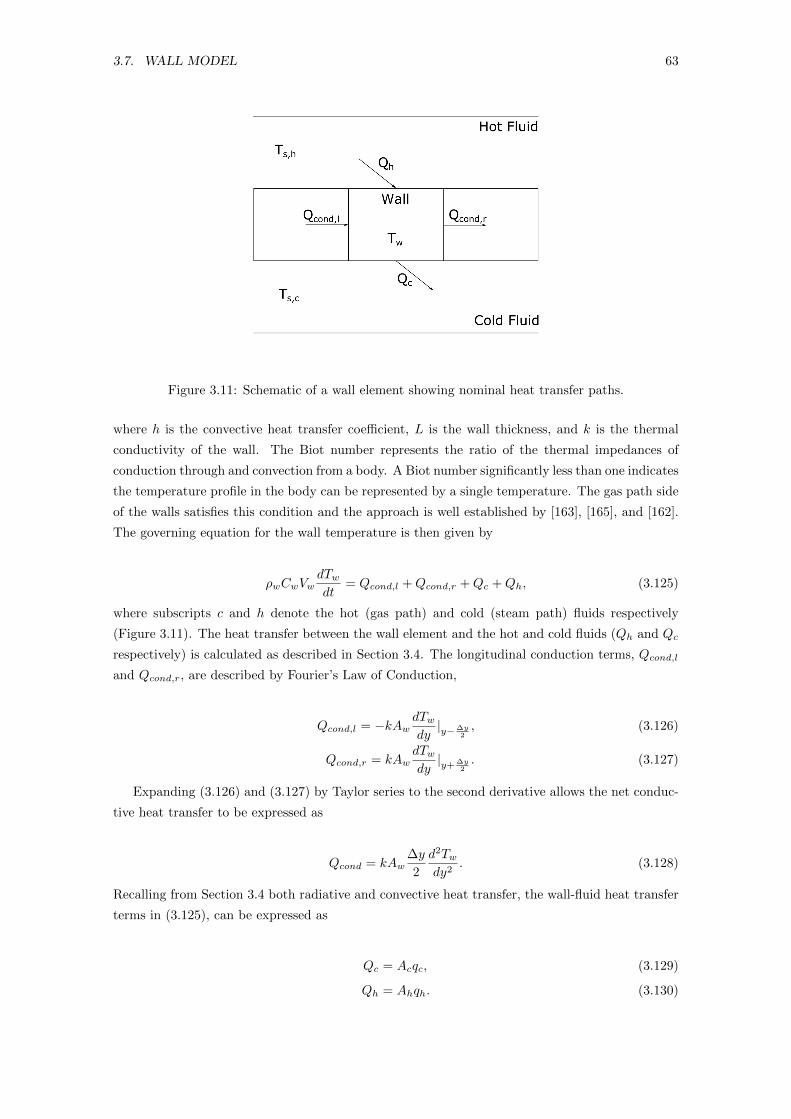
3.7. WALL MODEL 63
Figure 3.11: Schematic of a wall element showing nominal heat transfer paths.
where h is the convective heat transfer coefficient, L is the wall thickness, and k is the thermal
conductivity of the wall. The Biot number represents the ratio of the thermal impedances of
conduction through and convection from a body. A Biot number significantly less than one indicates
the temperature profile in the body can be represented by a single temperature. The gas path side
of the walls satisfies this condition and the approach is well established by [163], [165], and [162].
The governing equation for the wall temperature is then given by
ρwCwVwdTwdt
= Qcond,l +Qcond,r +Qc +Qh, (3.125)
where subscripts c and h denote the hot (gas path) and cold (steam path) fluids respectively
(Figure 3.11). The heat transfer between the wall element and the hot and cold fluids (Qh and Qc
respectively) is calculated as described in Section 3.4. The longitudinal conduction terms, Qcond,l
and Qcond,r, are described by Fourier’s Law of Conduction,
Qcond,l = −kAwdTwdy|y−∆y
2, (3.126)
Qcond,r = kAwdTwdy|y+ ∆y
2. (3.127)
Expanding (3.126) and (3.127) by Taylor series to the second derivative allows the net conduc-
tive heat transfer to be expressed as
Qcond = kAw∆y
2
d2Twdy2
. (3.128)
Recalling from Section 3.4 both radiative and convective heat transfer, the wall-fluid heat transfer
terms in (3.125), can be expressed as
Qc = Acqc, (3.129)
Qh = Ahqh. (3.130)
64 CHAPTER 3. DEVELOPMENT OF A DYNAMIC MODEL OF A BOILER
Figure 3.12: Schematic representation of heat transfer surface for the case of a tube with internal
heat transfer.
The heat transfer surface areas Ac and Ah can be expressed as
Ac = ∆ywc, (3.131)
Ah = ∆ywh, (3.132)
where w defines the ‘wetted’ perimeter of the heat transfer surface in contact with the fluid as
shown in Figure 3.12. The metal volume can similarly be expressed as
Vw = ∆yAw. (3.133)
Hence, (3.125) can be expressed as
ρwCwAwdTwdt
=kAw
2
d2Twdy2
+ wcqc + whqh. (3.134)
The boundary elements of a wall section are assumed to be well insulated. Hence the governing
equation for the left end boundary is
ρwCwVwdTwdt
= kAwdTwdy
∣∣∣∣∣y+ ∆y
2
+Qc +Qh, (3.135)
while the governing equation for the right end boundary is
ρwCwVwdTwdt
= −kAwdTwdy
∣∣∣∣∣y−∆y
2
+Qc +Qh, (3.136)
where the spatial derivatives of the wall temperature in (3.135) and (3.136) are evaluated numeri-
cally at the boundary location.
Under circumstances where the longitudinal conduction can be neglected, consideration of the
boundary elements is not required and (3.134) reduces to
dTwdt
=1
ρwCwAw(wcqc + whqh) . (3.137)
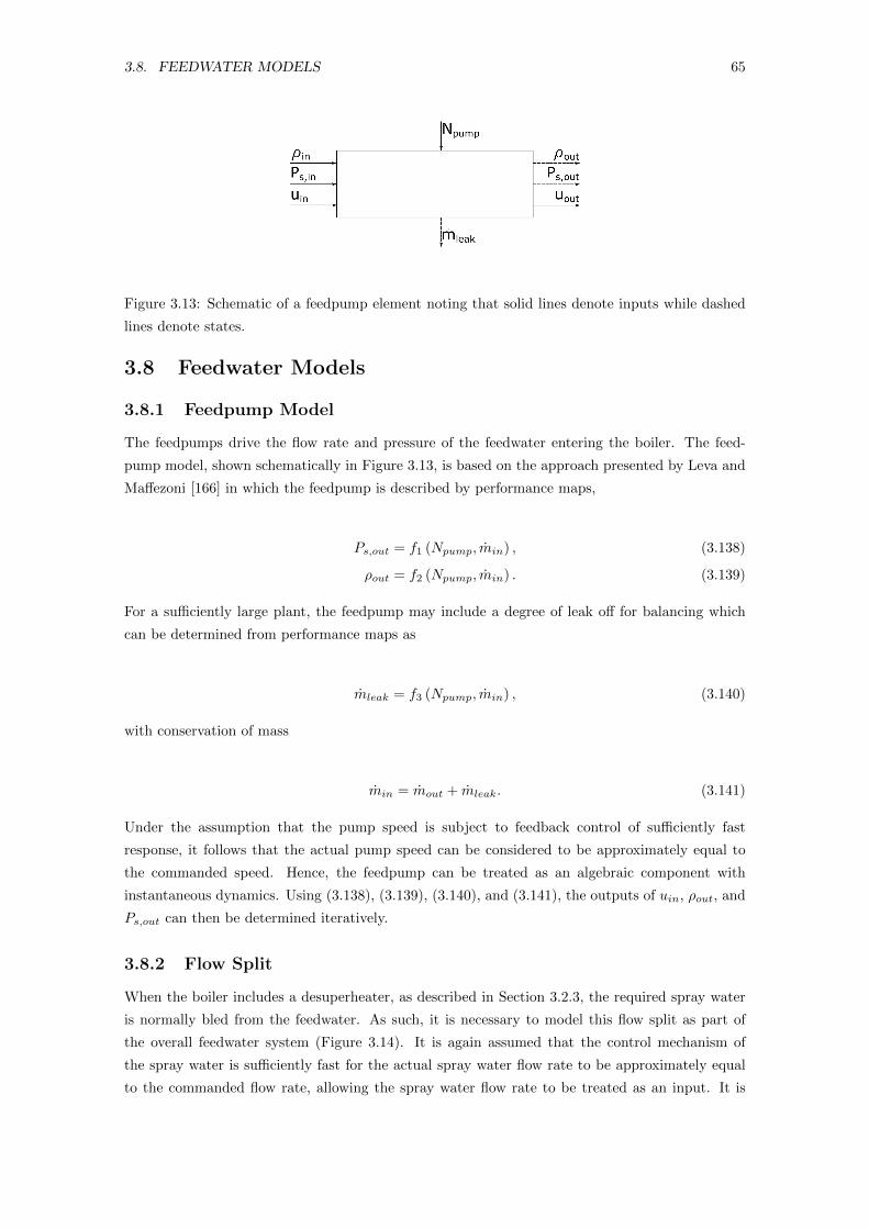
3.8. FEEDWATER MODELS 65
Figure 3.13: Schematic of a feedpump element noting that solid lines denote inputs while dashed
lines denote states.
3.8 Feedwater Models
3.8.1 Feedpump Model
The feedpumps drive the flow rate and pressure of the feedwater entering the boiler. The feed-
pump model, shown schematically in Figure 3.13, is based on the approach presented by Leva and
Maffezoni [166] in which the feedpump is described by performance maps,
Ps,out = f1 (Npump, min) , (3.138)
ρout = f2 (Npump, min) . (3.139)
For a sufficiently large plant, the feedpump may include a degree of leak off for balancing which
can be determined from performance maps as
mleak = f3 (Npump, min) , (3.140)
with conservation of mass
min = mout + mleak. (3.141)
Under the assumption that the pump speed is subject to feedback control of sufficiently fast
response, it follows that the actual pump speed can be considered to be approximately equal to
the commanded speed. Hence, the feedpump can be treated as an algebraic component with
instantaneous dynamics. Using (3.138), (3.139), (3.140), and (3.141), the outputs of uin, ρout, and
Ps,out can then be determined iteratively.
3.8.2 Flow Split
When the boiler includes a desuperheater, as described in Section 3.2.3, the required spray water
is normally bled from the feedwater. As such, it is necessary to model this flow split as part of
the overall feedwater system (Figure 3.14). It is again assumed that the control mechanism of
the spray water is sufficiently fast for the actual spray water flow rate to be approximately equal
to the commanded flow rate, allowing the spray water flow rate to be treated as an input. It is
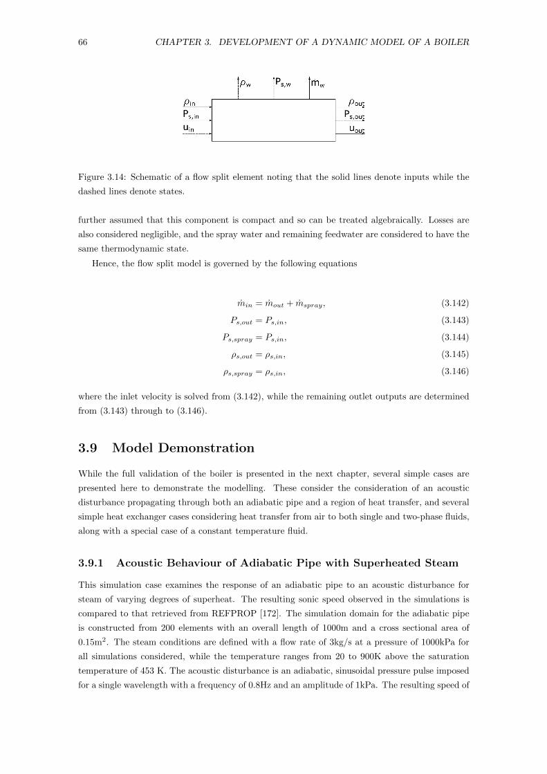
66 CHAPTER 3. DEVELOPMENT OF A DYNAMIC MODEL OF A BOILER
Figure 3.14: Schematic of a flow split element noting that the solid lines denote inputs while the
dashed lines denote states.
further assumed that this component is compact and so can be treated algebraically. Losses are
also considered negligible, and the spray water and remaining feedwater are considered to have the
same thermodynamic state.
Hence, the flow split model is governed by the following equations
min = mout + mspray, (3.142)
Ps,out = Ps,in, (3.143)
Ps,spray = Ps,in, (3.144)
ρs,out = ρs,in, (3.145)
ρs,spray = ρs,in, (3.146)
where the inlet velocity is solved from (3.142), while the remaining outlet outputs are determined
from (3.143) through to (3.146).
3.9 Model Demonstration
While the full validation of the boiler is presented in the next chapter, several simple cases are
presented here to demonstrate the modelling. These consider the consideration of an acoustic
disturbance propagating through both an adiabatic pipe and a region of heat transfer, and several
simple heat exchanger cases considering heat transfer from air to both single and two-phase fluids,
along with a special case of a constant temperature fluid.
3.9.1 Acoustic Behaviour of Adiabatic Pipe with Superheated Steam
This simulation case examines the response of an adiabatic pipe to an acoustic disturbance for
steam of varying degrees of superheat. The resulting sonic speed observed in the simulations is
compared to that retrieved from REFPROP [172]. The simulation domain for the adiabatic pipe
is constructed from 200 elements with an overall length of 1000m and a cross sectional area of
0.15m2. The steam conditions are defined with a flow rate of 3kg/s at a pressure of 1000kPa for
all simulations considered, while the temperature ranges from 20 to 900K above the saturation
temperature of 453 K. The acoustic disturbance is an adiabatic, sinusoidal pressure pulse imposed
for a single wavelength with a frequency of 0.8Hz and an amplitude of 1kPa. The resulting speed of
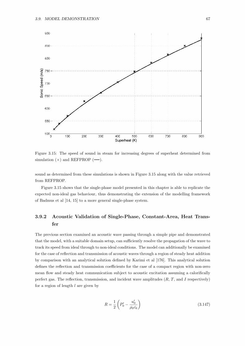
3.9. MODEL DEMONSTRATION 67
Figure 3.15: The speed of sound in steam for increasing degrees of superheat determined from
simulation (×) and REFPROP ( ).
sound as determined from these simulations is shown in Figure 3.15 along with the value retrieved
from REFPROP.
Figure 3.15 shows that the single-phase model presented in this chapter is able to replicate the
expected non-ideal gas behaviour, thus demonstrating the extension of the modelling framework
of Badmus et al [14, 15] to a more general single-phase system.
3.9.2 Acoustic Validation of Single-Phase, Constant-Area, Heat Trans-
fer
The previous section examined an acoustic wave passing through a simple pipe and demonstrated
that the model, with a suitable domain setup, can sufficiently resolve the propagation of the wave to
track its speed from ideal through to non-ideal conditions. The model can additionally be examined
for the case of reflection and transmission of acoustic waves through a region of steady heat addition
by comparison with an analytical solution defined by Karimi et al [176]. This analytical solution
defines the reflection and transmission coefficients for the case of a compact region with non-zero
mean flow and steady heat communication subject to acoustic excitation assuming a calorifically
perfect gas. The reflection, transmission, and incident wave amplitudes (R, T , and I respectively)
for a region of length l are given by
R =1
2
(P ′0 −
u′0ρ0c0
)(3.147)
68 CHAPTER 3. DEVELOPMENT OF A DYNAMIC MODEL OF A BOILER
I =1
2
(P ′0 +
u′0ρ0c0
)(3.148)
T =1
2
(P ′l +
u′lρlcl
)(3.149)
where the flow properties are expressed as superpositions of their steady and disturbance compo-
nents as ρ = ρ+ ρ′.
The analysis presented by Karimi et al [176] gives the relations between these wave amplitudes
for the case being considered as
T
I=a1d2 − a2d1
a1b2 − a2b1(3.150)
R
I=b2d1 − b1d2
a1b2 − a2b1(3.151)
where a1, a2, b1, b2, d1, and d2 are given by
a1 = −M20 + 2M0 − Ml
clc0
+ M0Mlclc0− 1 (3.152)
a2 =c0
γ − 1− γ
γ − 1M0c0 −
3
2M2
0 c0 +1
2M2l
c2lc0− 1
2M0M
2l
c2lc0
+1
2M3
0 c0 (3.153)
b1 = 1 +ρ0
ρl
c0clM0 (3.154)
b2 =cl
γ − 1+
γ
γ − 1Mlcl +
ρ0
ρlM0Mlc0 (3.155)
d1 = 1 + 2M0 − Mlclc0− M0Ml
clc0
+ M20 (3.156)
d2 =c0
γ − 1+
γ
γ − 1M0c0 −
3
2M2
0 c0 +1
2M2l
c2lc0− 1
2M3
0 c0 +1
2M0M
2l
c2lc0
(3.157)
and the Mach number, M , and heat capacity rate, c are given by
M =u
c(3.158)
c = mCp (3.159)
Two cases are examined based on a region of heat transfer of length 1 m and cross sectional
area of 0.01824m2. The first case considers a working fluid of pure nitrogen which is nominally
representative of both air and an ideal gas. The upstream conditions are 1 bar and 600 K while
the heat transfer is chosen to provide a downstream temperature of 2000 K. This keeps the test
case consistent with the conditions used by Karimi et al [176] and consistent with the analytic
solutions assumption of a calorifically perfect gas. The heat transfer is arbitrarily set rather than
determined from the heat transfer relations from section 3.4. This keeps the simulation consist
with the analytic case of steady heat transfer. A single acoustic pulse of frequency 10 Hz with
an amplitude of 1 kPa (1% of inlet pressure) is imposed to provide the acoustic excitation with a
wavelength of approximately 49.6 m based on upstream conditions ensuring that the region can
reasonably be considered compact. Upstream Mach numbers of 0.05, 0.1, and 0.15 are considered
with a comparison of the simulated and analytic results shown in figure 3.16. It can be seen that
the results show reasonable agreement between the simulated and analytic solutions.
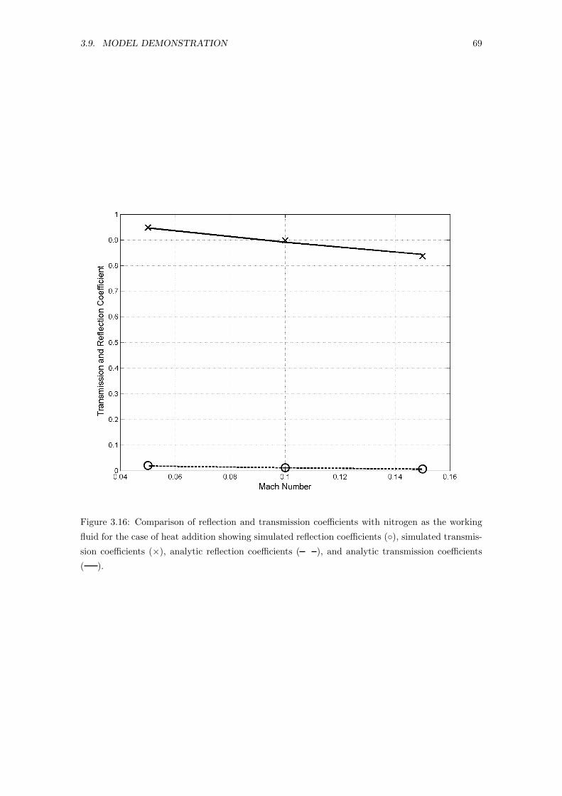
3.9. MODEL DEMONSTRATION 69
Figure 3.16: Comparison of reflection and transmission coefficients with nitrogen as the working
fluid for the case of heat addition showing simulated reflection coefficients (◦), simulated transmis-
sion coefficients (×), analytic reflection coefficients ( ), and analytic transmission coefficients
( ).
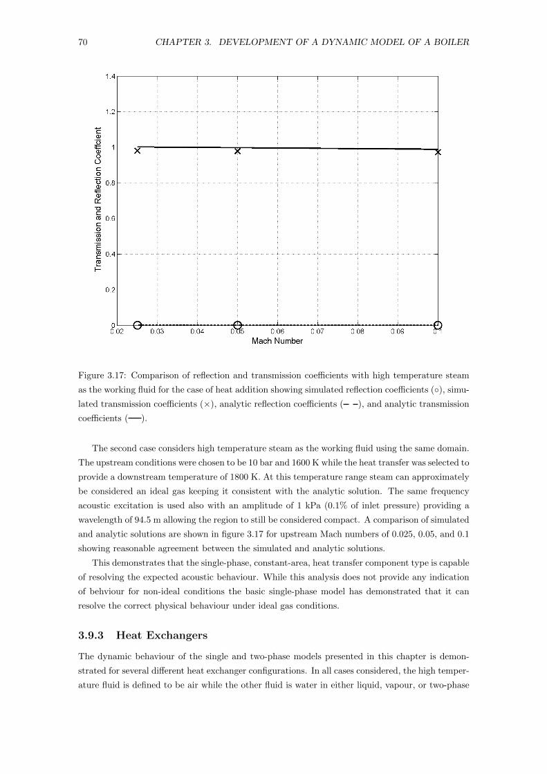
70 CHAPTER 3. DEVELOPMENT OF A DYNAMIC MODEL OF A BOILER
Figure 3.17: Comparison of reflection and transmission coefficients with high temperature steam
as the working fluid for the case of heat addition showing simulated reflection coefficients (◦), simu-
lated transmission coefficients (×), analytic reflection coefficients ( ), and analytic transmission
coefficients ( ).
The second case considers high temperature steam as the working fluid using the same domain.
The upstream conditions were chosen to be 10 bar and 1600 K while the heat transfer was selected to
provide a downstream temperature of 1800 K. At this temperature range steam can approximately
be considered an ideal gas keeping it consistent with the analytic solution. The same frequency
acoustic excitation is used also with an amplitude of 1 kPa (0.1% of inlet pressure) providing a
wavelength of 94.5 m allowing the region to still be considered compact. A comparison of simulated
and analytic solutions are shown in figure 3.17 for upstream Mach numbers of 0.025, 0.05, and 0.1
showing reasonable agreement between the simulated and analytic solutions.
This demonstrates that the single-phase, constant-area, heat transfer component type is capable
of resolving the expected acoustic behaviour. While this analysis does not provide any indication
of behviour for non-ideal conditions the basic single-phase model has demonstrated that it can
resolve the correct physical behaviour under ideal gas conditions.
3.9.3 Heat Exchangers
The dynamic behaviour of the single and two-phase models presented in this chapter is demon-
strated for several different heat exchanger configurations. In all cases considered, the high temper-
ature fluid is defined to be air while the other fluid is water in either liquid, vapour, or two-phase
3.9. MODEL DEMONSTRATION 71
Phase Steam/Water Conditions Air Conditions Length Vw
Acr Asurf hconv Acr Asurf hconv
(m2) (m2) (W/m2K) (m2) (m2) (W/m2K) (m) (m3)
Liquid 0.26 2180 5000 148 2750 200 80 13
Vapour 0.4 5790 500 148 7616 200 190 54
Two Phase 1 1933 50000 148 2333 200 60 35
Table 3.1: Geometry and heat transfer coefficients for the heat exchanger simulation cases
Phase Air Conditions Steam/Water Conditions
Ts,in Ps,in min Ts,in Ps,in min xin
(K) (kPa) (kg/s) (K) (kPa) (kg/s) (-)
Liquid 900 101.3 430 520 17000 360
Vapour 1600 101.3 430 640 16300 360
Two Phase 1700 101.3 430 622 16300 1640 0.05
Table 3.2: Upstream inlet fluid conditions for the heat exchanger simulation cases
conditions. Both counterflow and parallel-flow heat exchanger configurations are considered, with
the geometry and fluid conditions defined to be representative of a large scale boiler such as that
considered in the next chapter. While in a real system the lengths of each fluid path would nor-
mally be different, it will for simplicity be assumed that they are equal and that each is constructed
from 5 heat transfer elements linked by corresponding wall elements. It is also assumed that the
heat transfer coefficients are constant. The geometry and heat transfer coefficients for each phase
are shown in Table 3.1 while the upstream inlet fluid conditions used are shown in Table 3.2. In
all simulations the imposed transient is an increase in the upstream temperature of the gas path
by 100K over 7s.
The resulting, initial steady state temperature profiles are shown in Figures 3.18 and 3.19
for the counterflow and parallel-flow configurations respectively. The simulation results for the
outlet temperatures and the dryness fraction (if relevant) are shown in Figures 3.20 and 3.21.
The resulting profiles are qualitatively consistent with the expected behavior of counterflow and
parallel-flow heat exchangers [177, 178]. Similarly, the simulation results for the fluid path outlets
are qualitatively consistent with the dynamic behaviour shown by Roetzal and Xuan [179], Yin
and Jensen [180], and Romie [181].
3.9.4 Constant Temperature Fluid Heat Exchanger
An additional special heat exchanger case is examined where one of the fluids is constrained to have
constant temperature. Such a system can reasonable represent the behaviour of a heat exhanger
with a boiling or condensing fluid as seen in Figures 3.18 and 3.19. This examination includes
a comparison with an analytical solution for this case developed by Yin and Jensen [180]. This
set up is shown schematically in figure 3.22. The analytic model operates under the following
assumptions:
• The single-phase fluid and wall temperatures are functions of time and position only.
• There are no heat sources within the single-phase fluid or the wall.
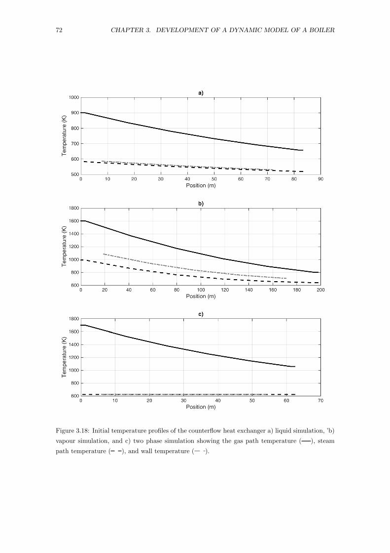
72 CHAPTER 3. DEVELOPMENT OF A DYNAMIC MODEL OF A BOILER
Figure 3.18: Initial temperature profiles of the counterflow heat exchanger a) liquid simulation, ’b)
vapour simulation, and c) two phase simulation showing the gas path temperature ( ), steam
path temperature ( ), and wall temperature ( ).
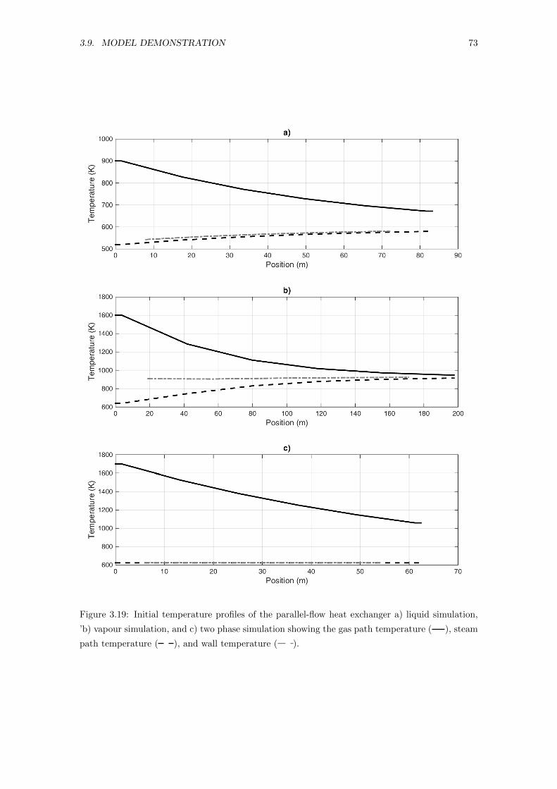
3.9. MODEL DEMONSTRATION 73
Figure 3.19: Initial temperature profiles of the parallel-flow heat exchanger a) liquid simulation,
’b) vapour simulation, and c) two phase simulation showing the gas path temperature ( ), steam
path temperature ( ), and wall temperature ( ).
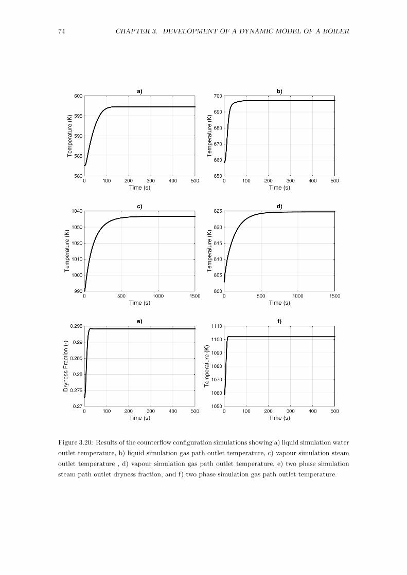
74 CHAPTER 3. DEVELOPMENT OF A DYNAMIC MODEL OF A BOILER
Figure 3.20: Results of the counterflow configuration simulations showing a) liquid simulation water
outlet temperature, b) liquid simulation gas path outlet temperature, c) vapour simulation steam
outlet temperature , d) vapour simulation gas path outlet temperature, e) two phase simulation
steam path outlet dryness fraction, and f) two phase simulation gas path outlet temperature.
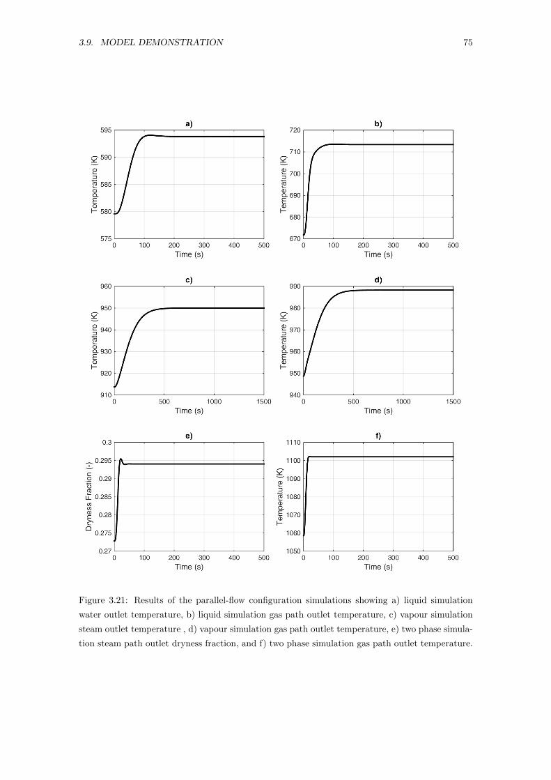
3.9. MODEL DEMONSTRATION 75
Figure 3.21: Results of the parallel-flow configuration simulations showing a) liquid simulation
water outlet temperature, b) liquid simulation gas path outlet temperature, c) vapour simulation
steam outlet temperature , d) vapour simulation gas path outlet temperature, e) two phase simula-
tion steam path outlet dryness fraction, and f) two phase simulation gas path outlet temperature.
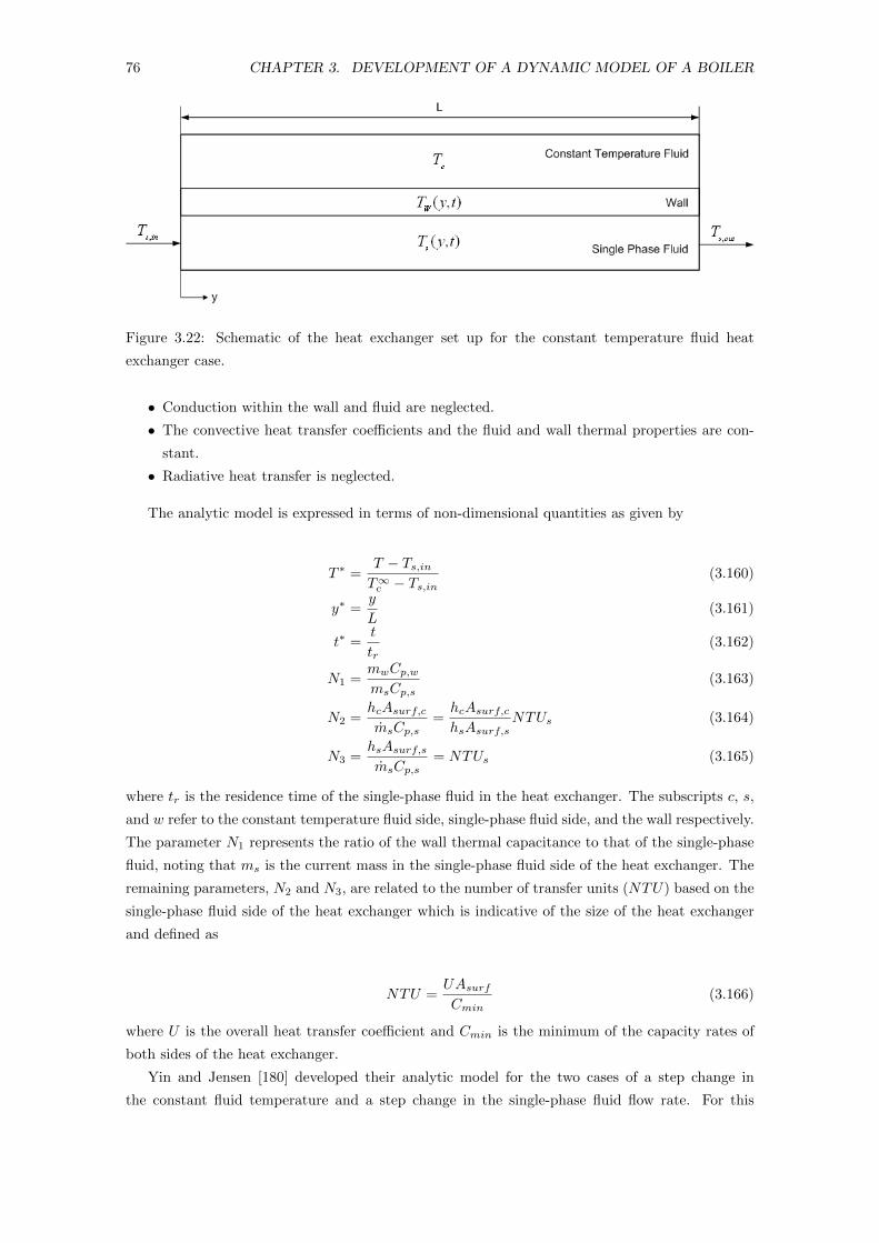
76 CHAPTER 3. DEVELOPMENT OF A DYNAMIC MODEL OF A BOILER
Figure 3.22: Schematic of the heat exchanger set up for the constant temperature fluid heat
exchanger case.
• Conduction within the wall and fluid are neglected.
• The convective heat transfer coefficients and the fluid and wall thermal properties are con-
stant.
• Radiative heat transfer is neglected.
The analytic model is expressed in terms of non-dimensional quantities as given by
T ∗ =T − Ts,inT∞c − Ts,in
(3.160)
y∗ =y
L(3.161)
t∗ =t
tr(3.162)
N1 =mwCp,wmsCp,s
(3.163)
N2 =hcAsurf,cmsCp,s
=hcAsurf,chsAsurf,s
NTUs (3.164)
N3 =hsAsurf,smsCp,s
= NTUs (3.165)
where tr is the residence time of the single-phase fluid in the heat exchanger. The subscripts c, s,
and w refer to the constant temperature fluid side, single-phase fluid side, and the wall respectively.
The parameter N1 represents the ratio of the wall thermal capacitance to that of the single-phase
fluid, noting that ms is the current mass in the single-phase fluid side of the heat exchanger. The
remaining parameters, N2 and N3, are related to the number of transfer units (NTU) based on the
single-phase fluid side of the heat exchanger which is indicative of the size of the heat exchanger
and defined as
NTU =UAsurfCmin
(3.166)
where U is the overall heat transfer coefficient and Cmin is the minimum of the capacity rates of
both sides of the heat exchanger.
Yin and Jensen [180] developed their analytic model for the two cases of a step change in
the constant fluid temperature and a step change in the single-phase fluid flow rate. For this
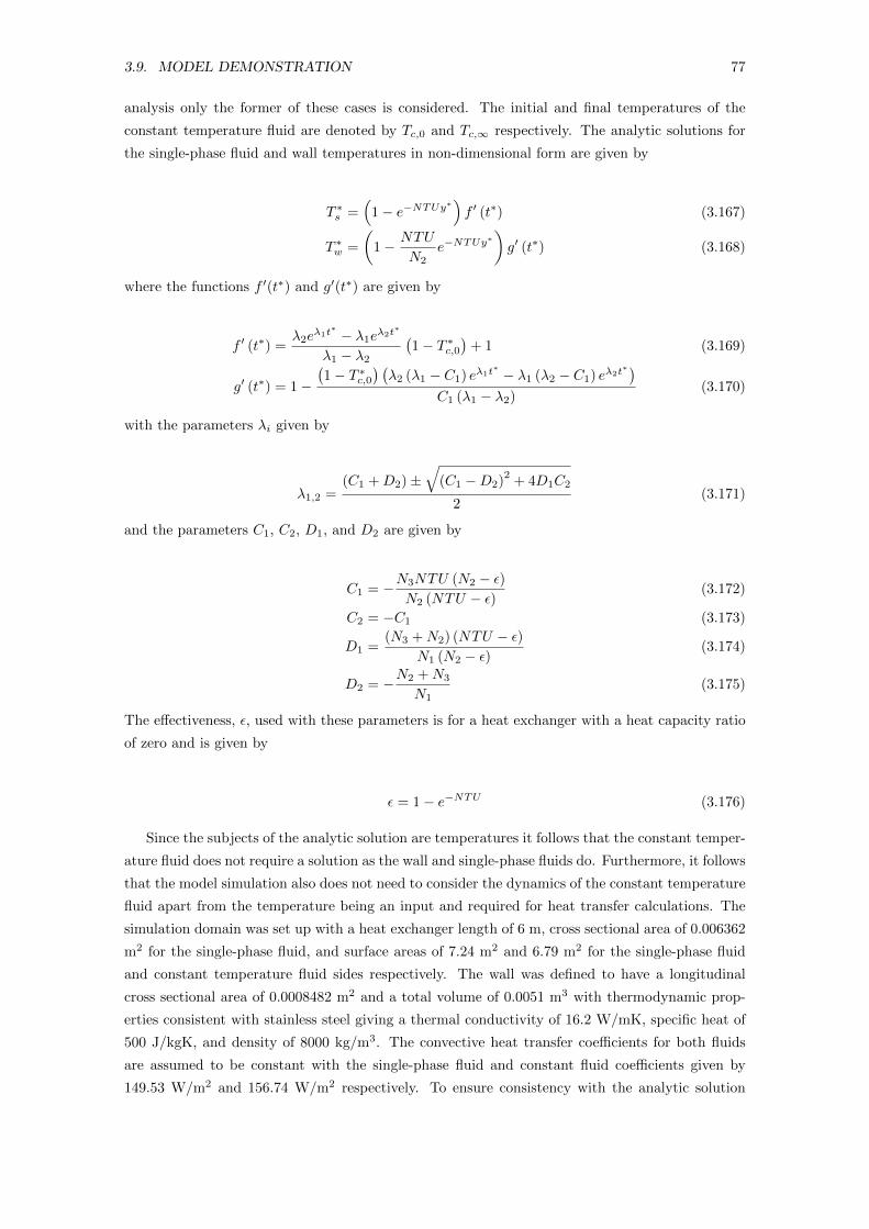
3.9. MODEL DEMONSTRATION 77
analysis only the former of these cases is considered. The initial and final temperatures of the
constant temperature fluid are denoted by Tc,0 and Tc,∞ respectively. The analytic solutions for
the single-phase fluid and wall temperatures in non-dimensional form are given by
T ∗s =(
1− e−NTUy∗)f ′ (t∗) (3.167)
T ∗w =
(1− NTU
N2e−NTUy
∗)g′ (t∗) (3.168)
where the functions f ′(t∗) and g′(t∗) are given by
f ′ (t∗) =λ2e
λ1t∗ − λ1e
λ2t∗
λ1 − λ2
(1− T ∗c,0
)+ 1 (3.169)
g′ (t∗) = 1−(1− T ∗c,0
) (λ2 (λ1 − C1) eλ1t
∗ − λ1 (λ2 − C1) eλ2t∗)
C1 (λ1 − λ2)(3.170)
with the parameters λi given by
λ1,2 =(C1 +D2)±
√(C1 −D2)
2+ 4D1C2
2(3.171)
and the parameters C1, C2, D1, and D2 are given by
C1 = −N3NTU (N2 − ε)N2 (NTU − ε)
(3.172)
C2 = −C1 (3.173)
D1 =(N3 +N2) (NTU − ε)
N1 (N2 − ε)(3.174)
D2 = −N2 +N3
N1(3.175)
The effectiveness, ε, used with these parameters is for a heat exchanger with a heat capacity ratio
of zero and is given by
ε = 1− e−NTU (3.176)
Since the subjects of the analytic solution are temperatures it follows that the constant temper-
ature fluid does not require a solution as the wall and single-phase fluids do. Furthermore, it follows
that the model simulation also does not need to consider the dynamics of the constant temperature
fluid apart from the temperature being an input and required for heat transfer calculations. The
simulation domain was set up with a heat exchanger length of 6 m, cross sectional area of 0.006362
m2 for the single-phase fluid, and surface areas of 7.24 m2 and 6.79 m2 for the single-phase fluid
and constant temperature fluid sides respectively. The wall was defined to have a longitudinal
cross sectional area of 0.0008482 m2 and a total volume of 0.0051 m3 with thermodynamic prop-
erties consistent with stainless steel giving a thermal conductivity of 16.2 W/mK, specific heat of
500 J/kgK, and density of 8000 kg/m3. The convective heat transfer coefficients for both fluids
are assumed to be constant with the single-phase fluid and constant fluid coefficients given by
149.53 W/m2 and 156.74 W/m2 respectively. To ensure consistency with the analytic solution
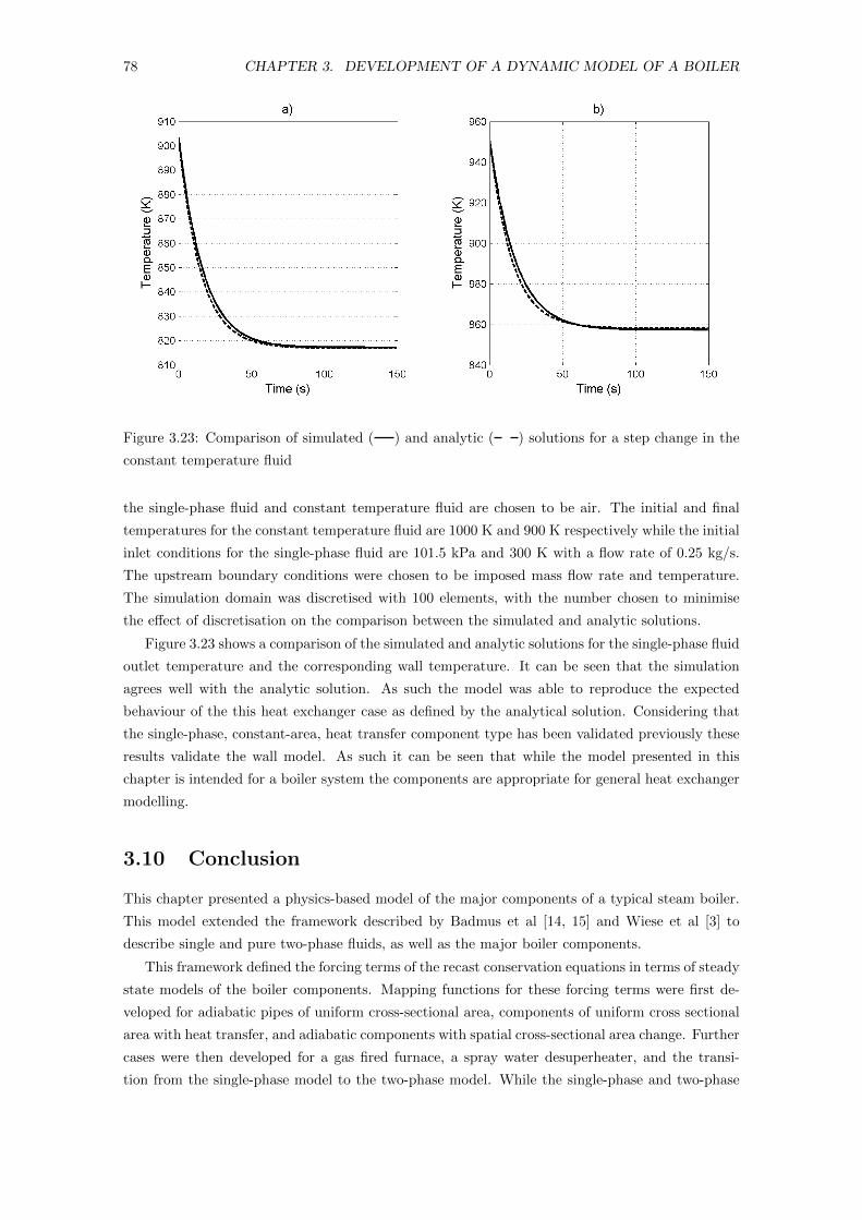
78 CHAPTER 3. DEVELOPMENT OF A DYNAMIC MODEL OF A BOILER
Figure 3.23: Comparison of simulated ( ) and analytic ( ) solutions for a step change in the
constant temperature fluid
the single-phase fluid and constant temperature fluid are chosen to be air. The initial and final
temperatures for the constant temperature fluid are 1000 K and 900 K respectively while the initial
inlet conditions for the single-phase fluid are 101.5 kPa and 300 K with a flow rate of 0.25 kg/s.
The upstream boundary conditions were chosen to be imposed mass flow rate and temperature.
The simulation domain was discretised with 100 elements, with the number chosen to minimise
the effect of discretisation on the comparison between the simulated and analytic solutions.
Figure 3.23 shows a comparison of the simulated and analytic solutions for the single-phase fluid
outlet temperature and the corresponding wall temperature. It can be seen that the simulation
agrees well with the analytic solution. As such the model was able to reproduce the expected
behaviour of the this heat exchanger case as defined by the analytical solution. Considering that
the single-phase, constant-area, heat transfer component type has been validated previously these
results validate the wall model. As such it can be seen that while the model presented in this
chapter is intended for a boiler system the components are appropriate for general heat exchanger
modelling.
3.10 Conclusion
This chapter presented a physics-based model of the major components of a typical steam boiler.
This model extended the framework described by Badmus et al [14, 15] and Wiese et al [3] to
describe single and pure two-phase fluids, as well as the major boiler components.
This framework defined the forcing terms of the recast conservation equations in terms of steady
state models of the boiler components. Mapping functions for these forcing terms were first de-
veloped for adiabatic pipes of uniform cross-sectional area, components of uniform cross sectional
area with heat transfer, and adiabatic components with spatial cross-sectional area change. Further
cases were then developed for a gas fired furnace, a spray water desuperheater, and the transi-
tion from the single-phase model to the two-phase model. While the single-phase and two-phase
3.10. CONCLUSION 79
models described most of the components in a boiler, not all components were compatible with
these models. Separate models were therefore developed for the steam drum, wall elements, and
the feedwater system. The boundary conditions, where appropriate, were defined by the LODI
conditions of Poinset and Lele [175].
While model development focused on a typical subcritical drum boiler, the approach is appli-
cable to a variety of systems provided that appropriate forcing term maps can be obtained. These
include a conventional heat exchanger or a supercritical boiler. The former was demonstrated in
this chapter by performing simulations on canonical test cases. The following chapter extends this
modelling to a complete, subcritical boiler of a large power plant.

80 CHAPTER 3. DEVELOPMENT OF A DYNAMIC MODEL OF A BOILER
Chapter 4
Validation of the Boiler Model
4.1 Introduction
A one-dimensional, physics based modelling approach was applied to components of a general
drum boiler in the previous chapter. This chapter presents a validation and subsequent analysis of
this modelling approach applied to the boiler of the 500MWe Newport power plant in Melbourne,
Australia. As part of this process, it is necessary to fit the geometry and model parameters.
While the geometry can be determined from available information, the heat transfer coefficients
and the parameters of the pressure drop relations, need to be fitted from the available data. The
opportunities for model reduction are then examined. This involves the simplification of the model
structure and the conversion of specific components to quasi-steady algebraic form. Additional
simplification of the governing equations and state models is also examined.
4.2 Modelling of the Newport Power Plant Boiler
4.2.1 Newport Power Plant
The Newport power plant is a 500 MWe natural gas-fired steam plant located in Melbourne,
Australia. It has been in operation since 1981 and currently serves as a peaker. It has a suspended,
forced circulation drum boiler with an economiser and four superheater stages; incorporating a
desuperheater between the third and fourth stages. The plant includes three main turbine stages
with an additional desuperheater and reheater between the high and intermediate pressure turbines.
While modelling of the turbines is beyond the scope of this work, consideration of the reheater and
its influence on the gas path is required. A schematic of the steam path of the boiler, showing the
available steam path data, is shown in Figure 4.1. Additional data includes the air and fuel flow
rates along with the inlet conditions for the gas path.
The structure of the gas path, along with the main steam path components, is shown in Figure
4.2. The gas path can be divided into three main sections: the furnace, and the front and rear
gas passes. An additional cavity encloses the steam drum. The waterwalls, or risers, form the
main structure and shell of the furnace and front gas pass, while the second stage superheater
forms the roof of both passes along with the main shell of the rear gas pass. The main steam path
components are mostly separated by header drums and in some cases additional connecting pipes.
81
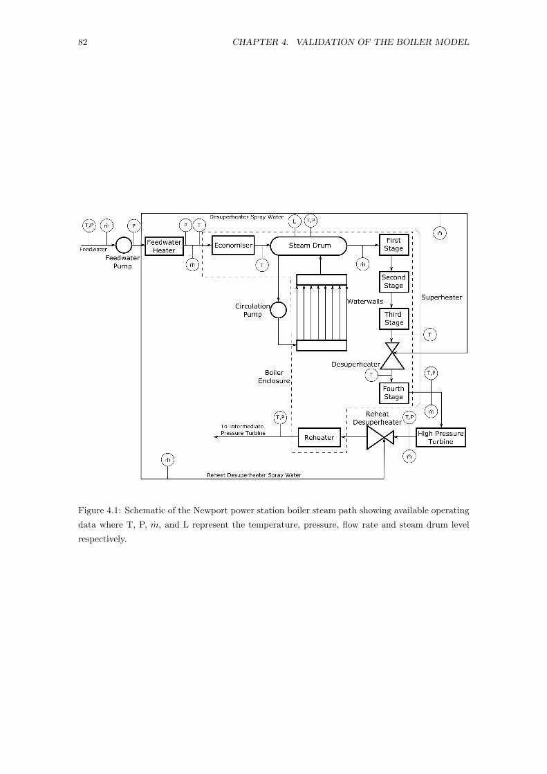
82 CHAPTER 4. VALIDATION OF THE BOILER MODEL
Figure 4.1: Schematic of the Newport power station boiler steam path showing available operating
data where T, P, m, and L represent the temperature, pressure, flow rate and steam drum level
respectively.
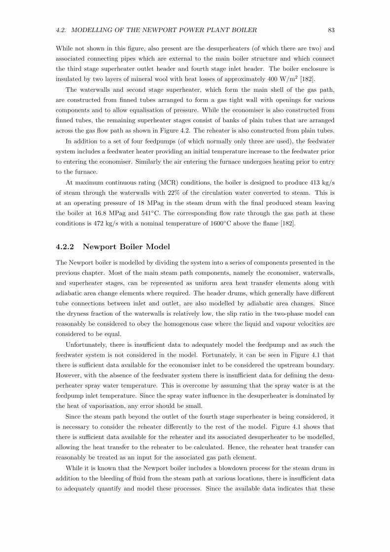
4.2. MODELLING OF THE NEWPORT POWER PLANT BOILER 83
While not shown in this figure, also present are the desuperheaters (of which there are two) and
associated connecting pipes which are external to the main boiler structure and which connect
the third stage superheater outlet header and fourth stage inlet header. The boiler enclosure is
insulated by two layers of mineral wool with heat losses of approximately 400 W/m2 [182].
The waterwalls and second stage superheater, which form the main shell of the gas path,
are constructed from finned tubes arranged to form a gas tight wall with openings for various
components and to allow equalisation of pressure. While the economiser is also constructed from
finned tubes, the remaining superheater stages consist of banks of plain tubes that are arranged
across the gas flow path as shown in Figure 4.2. The reheater is also constructed from plain tubes.
In addition to a set of four feedpumps (of which normally only three are used), the feedwater
system includes a feedwater heater providing an initial temperature increase to the feedwater prior
to entering the economiser. Similarly the air entering the furnace undergoes heating prior to entry
to the furnace.
At maximum continuous rating (MCR) conditions, the boiler is designed to produce 413 kg/s
of steam through the waterwalls with 22% of the circulation water converted to steam. This is
at an operating pressure of 18 MPag in the steam drum with the final produced steam leaving
the boiler at 16.8 MPag and 541◦C. The corresponding flow rate through the gas path at these
conditions is 472 kg/s with a nominal temperature of 1600◦C above the flame [182].
4.2.2 Newport Boiler Model
The Newport boiler is modelled by dividing the system into a series of components presented in the
previous chapter. Most of the main steam path components, namely the economiser, waterwalls,
and superheater stages, can be represented as uniform area heat transfer elements along with
adiabatic area change elements where required. The header drums, which generally have different
tube connections between inlet and outlet, are also modelled by adiabatic area changes. Since
the dryness fraction of the waterwalls is relatively low, the slip ratio in the two-phase model can
reasonably be considered to obey the homogenous case where the liquid and vapour velocities are
considered to be equal.
Unfortunately, there is insufficient data to adequately model the feedpump and as such the
feedwater system is not considered in the model. Fortunately, it can be seen in Figure 4.1 that
there is sufficient data available for the economiser inlet to be considered the upstream boundary.
However, with the absence of the feedwater system there is insufficient data for defining the desu-
perheater spray water temperature. This is overcome by assuming that the spray water is at the
feedpump inlet temperature. Since the spray water influence in the desuperheater is dominated by
the heat of vaporisation, any error should be small.
Since the steam path beyond the outlet of the fourth stage superheater is being considered, it
is necessary to consider the reheater differently to the rest of the model. Figure 4.1 shows that
there is sufficient data available for the reheater and its associated desuperheater to be modelled,
allowing the heat transfer to the reheater to be calculated. Hence, the reheater heat transfer can
reasonably be treated as an input for the associated gas path element.
While it is known that the Newport boiler includes a blowdown process for the steam drum in
addition to the bleeding of fluid from the steam path at various locations, there is insufficient data
to adequately quantify and model these processes. Since the available data indicates that these
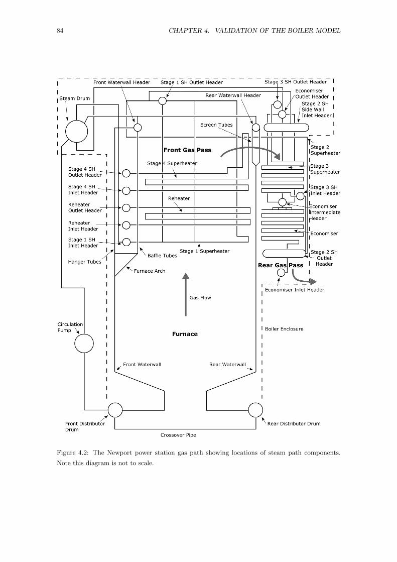
84 CHAPTER 4. VALIDATION OF THE BOILER MODEL
Figure 4.2: The Newport power station gas path showing locations of steam path components.
Note this diagram is not to scale.
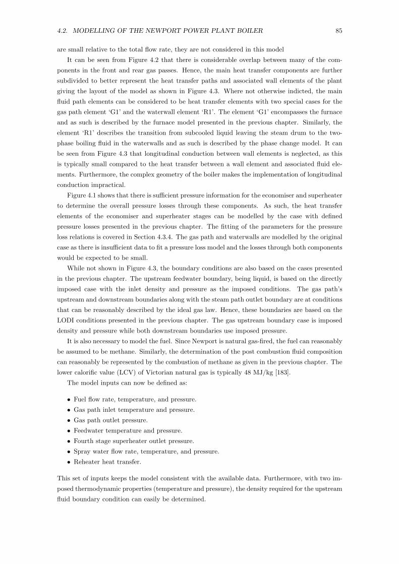
4.2. MODELLING OF THE NEWPORT POWER PLANT BOILER 85
are small relative to the total flow rate, they are not considered in this model
It can be seen from Figure 4.2 that there is considerable overlap between many of the com-
ponents in the front and rear gas passes. Hence, the main heat transfer components are further
subdivided to better represent the heat transfer paths and associated wall elements of the plant
giving the layout of the model as shown in Figure 4.3. Where not otherwise indicted, the main
fluid path elements can be considered to be heat transfer elements with two special cases for the
gas path element ‘G1’ and the waterwall element ‘R1’. The element ‘G1’ encompasses the furnace
and as such is described by the furnace model presented in the previous chapter. Similarly, the
element ‘R1’ describes the transition from subcooled liquid leaving the steam drum to the two-
phase boiling fluid in the waterwalls and as such is described by the phase change model. It can
be seen from Figure 4.3 that longitudinal conduction between wall elements is neglected, as this
is typically small compared to the heat transfer between a wall element and associated fluid ele-
ments. Furthermore, the complex geometry of the boiler makes the implementation of longitudinal
conduction impractical.
Figure 4.1 shows that there is sufficient pressure information for the economiser and superheater
to determine the overall pressure losses through these components. As such, the heat transfer
elements of the economiser and superheater stages can be modelled by the case with defined
pressure losses presented in the previous chapter. The fitting of the parameters for the pressure
loss relations is covered in Section 4.3.4. The gas path and waterwalls are modelled by the original
case as there is insufficient data to fit a pressure loss model and the losses through both components
would be expected to be small.
While not shown in Figure 4.3, the boundary conditions are also based on the cases presented
in the previous chapter. The upstream feedwater boundary, being liquid, is based on the directly
imposed case with the inlet density and pressure as the imposed conditions. The gas path’s
upstream and downstream boundaries along with the steam path outlet boundary are at conditions
that can be reasonably described by the ideal gas law. Hence, these boundaries are based on the
LODI conditions presented in the previous chapter. The gas upstream boundary case is imposed
density and pressure while both downstream boundaries use imposed pressure.
It is also necessary to model the fuel. Since Newport is natural gas-fired, the fuel can reasonably
be assumed to be methane. Similarly, the determination of the post combustion fluid composition
can reasonably be represented by the combustion of methane as given in the previous chapter. The
lower calorific value (LCV) of Victorian natural gas is typically 48 MJ/kg [183].
The model inputs can now be defined as:
• Fuel flow rate, temperature, and pressure.
• Gas path inlet temperature and pressure.
• Gas path outlet pressure.
• Feedwater temperature and pressure.
• Fourth stage superheater outlet pressure.
• Spray water flow rate, temperature, and pressure.
• Reheater heat transfer.
This set of inputs keeps the model consistent with the available data. Furthermore, with two im-
posed thermodynamic properties (temperature and pressure), the density required for the upstream
fluid boundary condition can easily be determined.
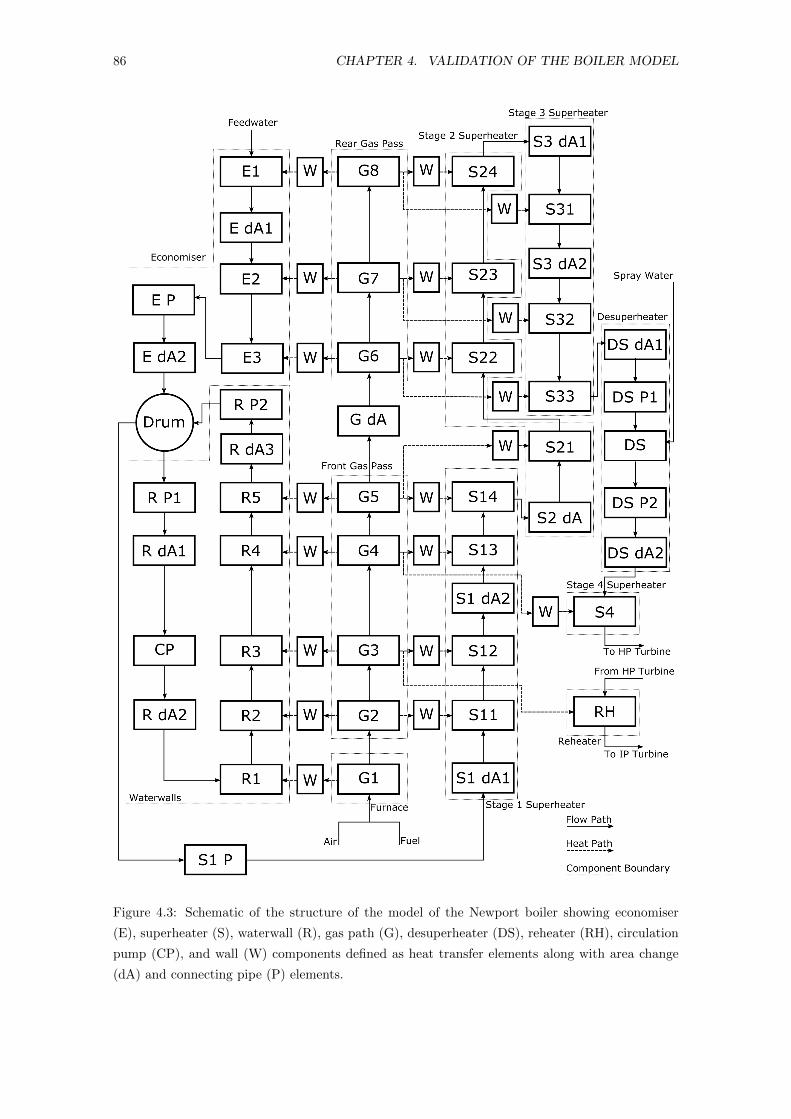
86 CHAPTER 4. VALIDATION OF THE BOILER MODEL
Figure 4.3: Schematic of the structure of the model of the Newport boiler showing economiser
(E), superheater (S), waterwall (R), gas path (G), desuperheater (DS), reheater (RH), circulation
pump (CP), and wall (W) components defined as heat transfer elements along with area change
(dA) and connecting pipe (P) elements.
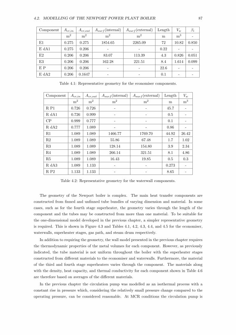
4.2. MODELLING OF THE NEWPORT POWER PLANT BOILER 87
Component Acr,in Acr,out Asurf (internal) Asurf (external) Length Vw βi
m2 m2 m2 m2 m m3 -
E1 0.275 0.275 1854.65 2265.09 72 10.82 0.850
E dA1 0.275 0.206 - - 0.22 - -
E2 0.206 0.206 83.07 113.39 4.3 0.826 0.051
E3 0.206 0.206 162.28 221.51 8.4 1.614 0.099
E P 0.206 0.206 - - 22.6 - -
E dA2 0.206 0.1647 - - 0.1 - -
Table 4.1: Representative geometry for the economiser components.
Component Acr,in Acr,out Asurf (internal) Asurf (external) Length Vw
m2 m2 m2 m2 m m3
R P1 0.726 0.726 - - 45.7 -
R dA1 0.726 0.999 - - 0.5 -
CP 0.999 0.777 - - 0.1 -
R dA2 0.777 1.089 - - 0.86 -
R1 1.089 1.089 1466.77 1769.70 44.92 26.42
R2 1.089 1.089 55.86 67.48 1.7 1.02
R3 1.089 1.089 128.14 154.80 3.9 2.34
R4 1.089 1.089 266.14 321.51 8.1 4.86
R5 1.089 1.089 16.43 19.85 0.5 0.3
R dA3 1.089 1.133 - - 0.273 -
R P2 1.133 1.133 - - 8.65 -
Table 4.2: Representative geometry for the waterwall components.
The geometry of the Newport boiler is complex. The main heat transfer components are
constructed from finned and unfinned tube bundles of varying dimension and material. In some
cases, such as for the fourth stage superheater, the geometry varies through the length of the
component and the tubes may be constructed from more than one material. To be suitable for
the one-dimensional model developed in the previous chapter, a simpler representative geometry
is required. This is shown in Figure 4.3 and Tables 4.1, 4.2, 4.3, 4.4, and 4.5 for the economiser,
waterwalls, superheater stages, gas path, and steam drum respectively.
In addition to requiring the geometry, the wall model presented in the previous chapter requires
the thermodynamic properties of the metal volumes for each component. However, as previously
indicated, the tube material is not uniform throughout the boiler with the superheater stages
constructed from different materials to the economiser and waterwalls. Furthermore, the material
of the third and fourth stage superheaters varies through the component. The materials along
with the density, heat capacity, and thermal conductivity for each component shown in Table 4.6
are therefore based on averages of the different materials.
In the previous chapter the circulation pump was modelled as an isothermal process with a
constant rise in pressure which, considering the relatively small pressure change compared to the
operating pressure, can be considered reasonable. At MCR conditions the circulation pump is
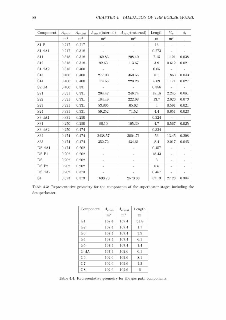
88 CHAPTER 4. VALIDATION OF THE BOILER MODEL
Component Acr,in Acr,out Asurf (internal) Asurf (external) Length Vw βi
m2 m2 m2 m2 m m3 -
S1 P 0.217 0.217 - - 16 - -
S1 dA1 0.217 0.318 - - 0.273 - -
S11 0.318 0.318 169.83 208.40 7.15 1.121 0.038
S12 0.318 0.318 92.63 113.67 3.9 0.612 0.021
S1 dA2 0.318 0.400 - - 0.05 - -
S13 0.400 0.400 277.90 350.55 8.1 1.863 0.043
S14 0.400 0.400 174.63 220.28 5.09 1.171 0.027
S2 dA 0.400 0.331 - - 0.356 - -
S21 0.331 0.331 204.42 246.74 15.18 2.245 0.081
S22 0.331 0.331 184.49 222.68 13.7 2.026 0.073
S23 0.331 0.331 53.865 65.02 4 0.591 0.021
S24 0.331 0.331 59.252 71.52 4.4 0.651 0.023
S3 dA1 0.331 0.250 - - 0.324 - -
S31 0.250 0.250 86.10 105.30 4.7 0.567 0.025
S3 dA2 0.250 0.474 - - 0.324 - -
S32 0.474 0.474 2438.57 3004.71 56 13.45 0.298
S33 0.474 0.474 352.72 434.61 8.4 2.017 0.045
DS dA1 0.474 0.202 - - 0.457 - -
DS P1 0.202 0.202 - - 18.43 - -
DS 0.202 0.202 - - 3 - -
DS P2 0.202 0.202 - - 6.5 - -
DS dA2 0.202 0.373 - - 0.457 - -
S4 0.373 0.373 1698.73 2573.38 57.13 27.23 0.304
Table 4.3: Representative geometry for the components of the superheater stages including the
desuperheater.
Component Acr,in Acr,out Length
m2 m2 m
G1 167.4 167.4 31.5
G2 167.4 167.4 1.7
G3 167.4 167.4 3.9
G4 167.4 167.4 6.1
G5 167.4 167.4 1.4
G dA 167.4 102.6 0.1
G6 102.6 102.6 8.1
G7 102.6 102.6 4.3
G8 102.6 102.6 6
Table 4.4: Representative geometry for the gas path components.
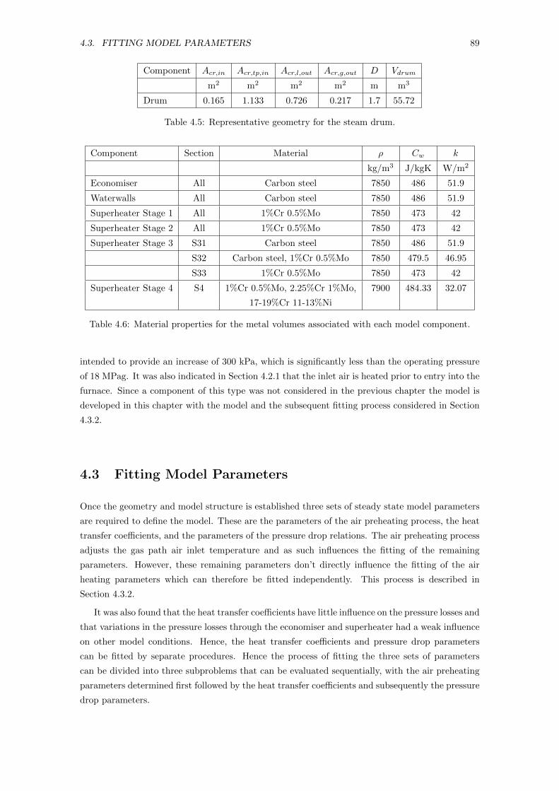
4.3. FITTING MODEL PARAMETERS 89
Component Acr,in Acr,tp,in Acr,l,out Acr,g,out D Vdrum
m2 m2 m2 m2 m m3
Drum 0.165 1.133 0.726 0.217 1.7 55.72
Table 4.5: Representative geometry for the steam drum.
Component Section Material ρ Cw k
kg/m3 J/kgK W/m2
Economiser All Carbon steel 7850 486 51.9
Waterwalls All Carbon steel 7850 486 51.9
Superheater Stage 1 All 1%Cr 0.5%Mo 7850 473 42
Superheater Stage 2 All 1%Cr 0.5%Mo 7850 473 42
Superheater Stage 3 S31 Carbon steel 7850 486 51.9
S32 Carbon steel, 1%Cr 0.5%Mo 7850 479.5 46.95
S33 1%Cr 0.5%Mo 7850 473 42
Superheater Stage 4 S4 1%Cr 0.5%Mo, 2.25%Cr 1%Mo, 7900 484.33 32.07
17-19%Cr 11-13%Ni
Table 4.6: Material properties for the metal volumes associated with each model component.
intended to provide an increase of 300 kPa, which is significantly less than the operating pressure
of 18 MPag. It was also indicated in Section 4.2.1 that the inlet air is heated prior to entry into the
furnace. Since a component of this type was not considered in the previous chapter the model is
developed in this chapter with the model and the subsequent fitting process considered in Section
4.3.2.
4.3 Fitting Model Parameters
Once the geometry and model structure is established three sets of steady state model parameters
are required to define the model. These are the parameters of the air preheating process, the heat
transfer coefficients, and the parameters of the pressure drop relations. The air preheating process
adjusts the gas path air inlet temperature and as such influences the fitting of the remaining
parameters. However, these remaining parameters don’t directly influence the fitting of the air
heating parameters which can therefore be fitted independently. This process is described in
Section 4.3.2.
It was also found that the heat transfer coefficients have little influence on the pressure losses and
that variations in the pressure losses through the economiser and superheater had a weak influence
on other model conditions. Hence, the heat transfer coefficients and pressure drop parameters
can be fitted by separate procedures. Hence the process of fitting the three sets of parameters
can be divided into three subproblems that can be evaluated sequentially, with the air preheating
parameters determined first followed by the heat transfer coefficients and subsequently the pressure
drop parameters.
90 CHAPTER 4. VALIDATION OF THE BOILER MODEL
4.3.1 Steady State Model Calculation
As part of the subsequent evaluation of the model parameters the evaluation of the overall steady
state is required. The inputs to the model for the overall steady state calculation are:
• Economiser inlet temperature and pressure.
• Gas path inlet temperature, pressure and flow rate.
• Fuel temperature, pressure, and flow rate.
• Desuperheater spray water flow rate, temperature, and pressure.
• Reheater heat transfer.
The overall steady state of the model is determined by a process with multiple levels of iterative
calculations, each using the Newton-Raphson method, down to each individual element in Figure
4.3. At the outermost level the system is divided into two sections based on the gas path. The
first section encompasses the furnace and front gas pass along with its associated steam path
components including the steam drum and desuperheater. The second section is the rear gas path
and corresponding components. From Figure 4.3 it can be seen that the economiser and third stage
superheater outlet temperature and pressure form the iterative variables linking the two sections
The evaluation of the furnace and front gas pass section and the rear gas pass section form the
next tier down. The evaluation of the furnace and front gas pass section also involves a multiple
level iterative process with the outermost level determining the feedwater mass flow rate, which at
steady state is equivalent to the steam generated through the riser.
A further, subordinate iterative process is required to evaluate the steam drum and associated
components. This process iterates on the drum two-phase inlet pressure, Ps,drum,tp,in, to match
drum and riser conditions.
The evaluation of the gas path components and associated steam path components requires
the iterative determination of the wall temperatures linking each steam path component to its
corresponding gas path component. Fortunately components G1 to G5 and the associated steam
path components (see Figure 4.3) can be evaluated sequentially, as at this level each component
is independent of the later components. This process additionally includes the determination of
the relevant connecting components such as area changes shown in Figure 4.3. The details for the
evaluation of the individual components, which are themselves solved iteratively, can be found in
Appendix A.
Returning to the uppermost tier, the evaluation of the rear gas pass section requires the iterative
determination of the wall temperatures linking the relevant steam and gas path components. It can
be seen in Figure 4.3 that the economiser and third stage superheater are, in a one dimensional
sense, arranged in a counterflow configuration. Hence the components cannot be evaluated in
a sequential process like the furnace and front gas pass components. Hence, the relevant wall
temperatures form an iterative vector allowing each fluid path to be considered separately.
The details of the steady state evaluation process along with the details for the evaluation of
each individual fluid component can be found in Appendix B. Through this process the overall
steady state of the system can be determined for use in both the fitting of parameters covered in
subsequent sections and determining the initial condition for simulations.
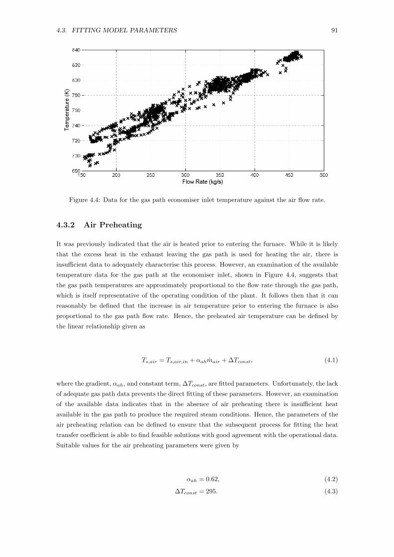
4.3. FITTING MODEL PARAMETERS 91
Figure 4.4: Data for the gas path economiser inlet temperature against the air flow rate.
4.3.2 Air Preheating
It was previously indicated that the air is heated prior to entering the furnace. While it is likely
that the excess heat in the exhaust leaving the gas path is used for heating the air, there is
insufficient data to adequately characterise this process. However, an examination of the available
temperature data for the gas path at the economiser inlet, shown in Figure 4.4, suggests that
the gas path temperatures are approximately proportional to the flow rate through the gas path,
which is itself representative of the operating condition of the plant. It follows then that it can
reasonably be defined that the increase in air temperature prior to entering the furnace is also
proportional to the gas path flow rate. Hence, the preheated air temperature can be defined by
the linear relationship given as
Ts,air = Ts,air,in + αahmair + ∆Tconst, (4.1)
where the gradient, αah, and constant term, ∆Tconst, are fitted parameters. Unfortunately, the lack
of adequate gas path data prevents the direct fitting of these parameters. However, an examination
of the available data indicates that in the absence of air preheating there is insufficient heat
available in the gas path to produce the required steam conditions. Hence, the parameters of the
air preheating relation can be defined to ensure that the subsequent process for fitting the heat
transfer coefficient is able to find feasible solutions with good agreement with the operational data.
Suitable values for the air preheating parameters were given by
αah = 0.62, (4.2)
∆Tconst = 295. (4.3)
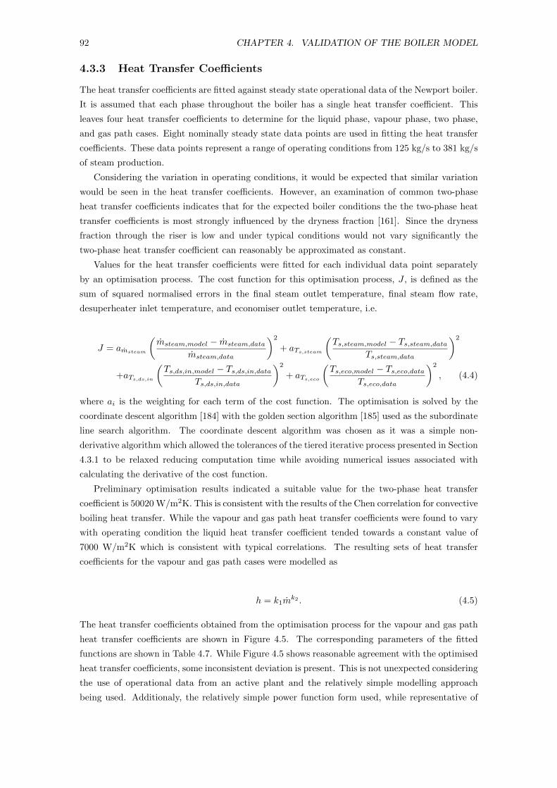
92 CHAPTER 4. VALIDATION OF THE BOILER MODEL
4.3.3 Heat Transfer Coefficients
The heat transfer coefficients are fitted against steady state operational data of the Newport boiler.
It is assumed that each phase throughout the boiler has a single heat transfer coefficient. This
leaves four heat transfer coefficients to determine for the liquid phase, vapour phase, two phase,
and gas path cases. Eight nominally steady state data points are used in fitting the heat transfer
coefficients. These data points represent a range of operating conditions from 125 kg/s to 381 kg/s
of steam production.
Considering the variation in operating conditions, it would be expected that similar variation
would be seen in the heat transfer coefficients. However, an examination of common two-phase
heat transfer coefficients indicates that for the expected boiler conditions the the two-phase heat
transfer coefficients is most strongly influenced by the dryness fraction [161]. Since the dryness
fraction through the riser is low and under typical conditions would not vary significantly the
two-phase heat transfer coefficient can reasonably be approximated as constant.
Values for the heat transfer coefficients were fitted for each individual data point separately
by an optimisation process. The cost function for this optimisation process, J , is defined as the
sum of squared normalised errors in the final steam outlet temperature, final steam flow rate,
desuperheater inlet temperature, and economiser outlet temperature, i.e.
J = amsteam
(msteam,model − msteam,data
msteam,data
)2
+ aTs,steam
(Ts,steam,model − Ts,steam,data
Ts,steam,data
)2
+aTs,ds,in
(Ts,ds,in,model − Ts,ds,in,data
Ts,ds,in,data
)2
+ aTs,eco
(Ts,eco,model − Ts,eco,data
Ts,eco,data
)2
, (4.4)
where ai is the weighting for each term of the cost function. The optimisation is solved by the
coordinate descent algorithm [184] with the golden section algorithm [185] used as the subordinate
line search algorithm. The coordinate descent algorithm was chosen as it was a simple non-
derivative algorithm which allowed the tolerances of the tiered iterative process presented in Section
4.3.1 to be relaxed reducing computation time while avoiding numerical issues associated with
calculating the derivative of the cost function.
Preliminary optimisation results indicated a suitable value for the two-phase heat transfer
coefficient is 50020 W/m2K. This is consistent with the results of the Chen correlation for convective
boiling heat transfer. While the vapour and gas path heat transfer coefficients were found to vary
with operating condition the liquid heat transfer coefficient tended towards a constant value of
7000 W/m2K which is consistent with typical correlations. The resulting sets of heat transfer
coefficients for the vapour and gas path cases were modelled as
h = k1mk2 . (4.5)
The heat transfer coefficients obtained from the optimisation process for the vapour and gas path
heat transfer coefficients are shown in Figure 4.5. The corresponding parameters of the fitted
functions are shown in Table 4.7. While Figure 4.5 shows reasonable agreement with the optimised
heat transfer coefficients, some inconsistent deviation is present. This is not unexpected considering
the use of operational data from an active plant and the relatively simple modelling approach
being used. Additionaly, the relatively simple power function form used, while representative of
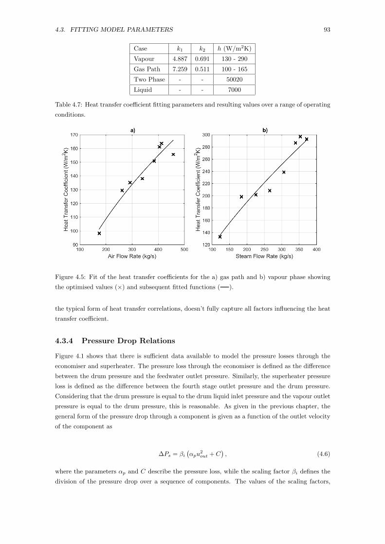
4.3. FITTING MODEL PARAMETERS 93
Case k1 k2 h (W/m2K)
Vapour 4.887 0.691 130 - 290
Gas Path 7.259 0.511 100 - 165
Two Phase - - 50020
Liquid - - 7000
Table 4.7: Heat transfer coefficient fitting parameters and resulting values over a range of operating
conditions.
Figure 4.5: Fit of the heat transfer coefficients for the a) gas path and b) vapour phase showing
the optimised values (×) and subsequent fitted functions ( ).
the typical form of heat transfer correlations, doesn’t fully capture all factors influencing the heat
transfer coefficient.
4.3.4 Pressure Drop Relations
Figure 4.1 shows that there is sufficient data available to model the pressure losses through the
economiser and superheater. The pressure loss through the economiser is defined as the difference
between the drum pressure and the feedwater outlet pressure. Similarly, the superheater pressure
loss is defined as the difference between the fourth stage outlet pressure and the drum pressure.
Considering that the drum pressure is equal to the drum liquid inlet pressure and the vapour outlet
pressure is equal to the drum pressure, this is reasonable. As given in the previous chapter, the
general form of the pressure drop through a component is given as a function of the outlet velocity
of the component as
∆Ps = βi(αpu
2out + C
), (4.6)
where the parameters αp and C describe the pressure loss, while the scaling factor βi defines the
division of the pressure drop over a sequence of components. The values of the scaling factors,
94 CHAPTER 4. VALIDATION OF THE BOILER MODEL
Component αp C
Economiser 111.604 414
Superheater 5.442 0
Table 4.8: Fitted pressure drop parameters for the economiser and superheater.
the calculation of which was defined in the previous chapter, for the superheater and economiser
components are shown in Tables 4.3 and 4.1 respectively.
As indicated earlier, the parameters of the pressure drop relations for the economiser and
superheater stages are fitted separately to the process for the heat transfer coefficients. This is
reasonable since fitting the heat transfer coefficients was found to have little influence on the
pressure. Similarly, variations in the pressure drop through the economiser and superheater were
found to have only a minor influence on other model conditions.
An examination of the operational data indicates that suitable values for the constant term in
(4.6) can be determined for both the economiser and superheater as shown in Table 4.8. While
the constant term for the superheater is 0 as would be expected, the pressure loss through the
economiser shows a significant additional pressure loss independent of the velocity. While the
exact source of this pressure loss is uncertain, it is possibly due to unaccounted for losses in the
steam drum or feedwater system.
The gradient terms for the economiser and superheater pressure loss relations are fitted by
separate optimisation processes evaluate sequentially with the economsier considered first. The
same previously used eight data points with suitably fitted heat transfer coefficients are considered
in these optimisations. Since the only parameter being fitted in each case is the gradient, the
golden section algorithm is used. The cost functions for fitting the economiser and superheater
pressure drop relations are defined as the sum of the squared normalised errors over the set of data
points
Jeco =
N∑i=1
(Ps,drum,model,i − Ps,drum,data,i
Ps,drum,data,i
)2
, (4.7)
Jsh =
N∑i=1
(Ps,steam,model,i − Ps,steam,data,i
Ps,steam,data,i
)2
. (4.8)
The resulting parameters for the pressure drop relations for the economiser and superheater are
shown in Table 4.8.
4.3.5 Steady State Results
With the fitted heat transfer coefficient and pressure drop relations, the error between the model
and data is shown in Figures 4.6 and 4.7 in percentage terms relative to the data, with both the
set of eight data points considered and an additional set of fifteen data points over the same range
as the validation set. It can be seen that overall the model achieves good agreement with data.
In particular, the pressure drop relations are able to achieve errors of less than 1%. Additionally,
Figure 4.6 shows that the model achieves good agreement with the final steam stagnation enthalpy
which, in combination with the good agreement with pressure, ensures that the model would
4.4. DYNAMIC ANALYSIS 95
provide suitable upstream conditions for the high pressure steam turbine if used in a full power
plant model.
While the model shows good overall agreement, Figure 4.7 nonetheless shows that some of the
errors at intermediate stages throughout the boiler show a degree of bias, such as for the economiser
outlet temperature. Similarly, some errors show trends as the operating conditions varies, such as
can be seen with the desuperheater inlet temperature and final steam temperature. However, since
the overall errors have been demonstrated to be low, the model can be considered representative
of the Newport boiler at steady state.
4.4 Dynamic Analysis
The model of the Newport boiler is simulated over a 10890s transient from a moderately high op-
erating condition generating 300kg/s of steam to a moderately low operating condition generating
just below 200kg/s of steam. The operational data available for the Newport boiler is sampled
at 30s increments. The model is simulated using a variable step implicit solver with smaller time
steps than available from the operational data permitted. As such model inputs at intermediate
instants are described by cubic splines, which ensures smooth gradients between data points.
The simulation inputs describing the transient being considered are shown in Figure 4.8. While
the majority of the inputs are obtained from the operational data, such data is not available for
the gas path inlet pressure, gas path outlet pressure, and the fuel temperature. It can reasonably
be assumed that the gas path inlet pressure is atmospheric and the fuel temperature equal to the
unheated air temperature. While the pressure loss through the gas path would be expected to
be small, the choice of upstream and downstream boundary conditions requires that this loss be
accounted for to ensure correct numerical behaviour. Hence, a quasi-steady gas path downstream
pressure is imposed based on the steady state evaluation as presented in Section 4.3.1. The imposed
downstream pressures inputs are shown in Figure 4.9.
The simulation results for the representative Newport model show that the model achieves
good overall agreement with the operational data. In particular the drum pressure and the gas
path flow rate show exceptionally good agreement. The final steam flow rate shows generally
good agreement, with the exception of some oscillatory behaviour not found in the corresponding
operational data. However, this oscillatory behaviour matches up with oscillations in the fuel flow
rate input data shown in Figure 4.8. Hence, this is not numerical but indicates that it is likely
that there is some form of damping in either the plant or the flow rate measurement not accounted
for in the model. However, the resulting error is small and the main dynamics are captured
well. Similarly, the desuperheater inlet and outlet temperatures show that the model captures the
overall dynamics fairly well. The economiser outlet temperature shows more significant errors, as
would be expected considering the steady state results shown previously in Figure 4.7. Figure 4.11
shows that the model doesn’t achieve as good agreement with the drum level dynamics with the
oscillatory behaviour not captured and the model results showing a deviation away from the mean
value. However the error remains well within 10% over most of the simulation allowing it to still
be indicative of significant drum level deviations.
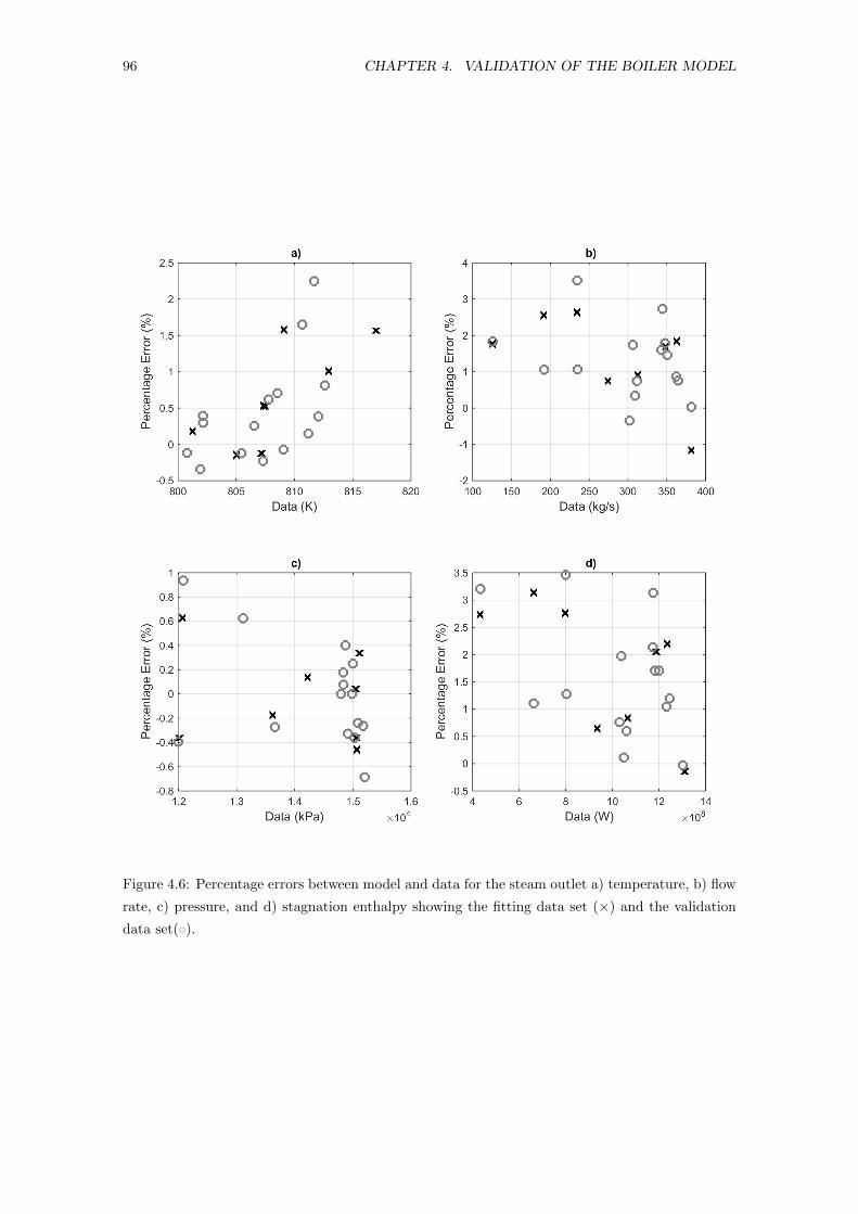
96 CHAPTER 4. VALIDATION OF THE BOILER MODEL
Figure 4.6: Percentage errors between model and data for the steam outlet a) temperature, b) flow
rate, c) pressure, and d) stagnation enthalpy showing the fitting data set (×) and the validation
data set(◦).
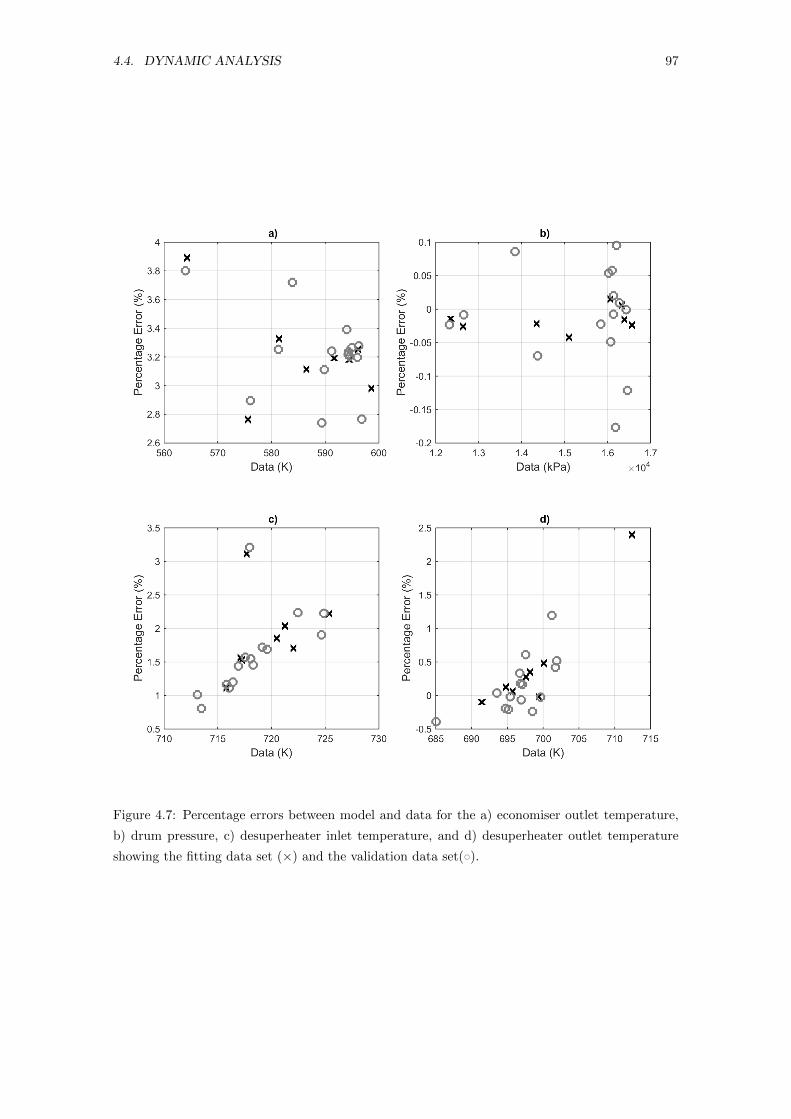
4.4. DYNAMIC ANALYSIS 97
Figure 4.7: Percentage errors between model and data for the a) economiser outlet temperature,
b) drum pressure, c) desuperheater inlet temperature, and d) desuperheater outlet temperature
showing the fitting data set (×) and the validation data set(◦).
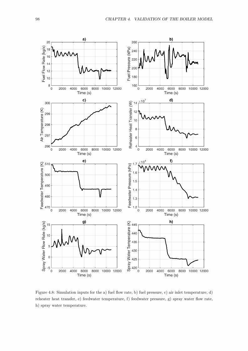
98 CHAPTER 4. VALIDATION OF THE BOILER MODEL
Figure 4.8: Simulation inputs for the a) fuel flow rate, b) fuel pressure, c) air inlet temperature, d)
reheater heat transfer, e) feedwater temperature, f) feedwater pressure, g) spray water flow rate,
h) spray water temperature.
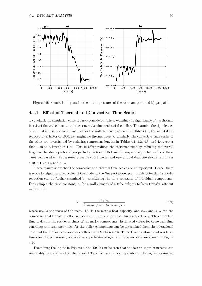
4.4. DYNAMIC ANALYSIS 99
Figure 4.9: Simulation inputs for the outlet pressures of the a) steam path and b) gas path.
4.4.1 Effect of Thermal and Convective Time Scales
Two additional simulation cases are now considered. These examine the significance of the thermal
inertia of the wall elements and the convective time scales of the boiler. To examine the significance
of thermal inertia, the metal volumes for the wall elements presented in Tables 4.1, 4.2, and 4.3 are
reduced by a factor of 1000, i.e. negligible thermal inertia. Similarly, the convective time scales of
the plant are investigated by reducing component lengths in Tables 4.1, 4.2, 4.3, and 4.4 greater
than 1 m to a length of 1 m. This in effect reduces the residence time by reducing the overall
length of the steam path and gas paths by factors of 15.1 and 7.6 respectively. The results of these
cases compared to the representative Newport model and operational data are shown in Figures
4.10, 4.11, 4.12, and 4.13.
These results show that the convective and thermal time scales are unimportant. Hence, there
is scope for significant reduction of the model of the Newport power plant. This potential for model
reduction can be further examined by considering the time constants of individual components.
For example the time constant, τ , for a wall element of a tube subject to heat transfer without
radiation is
τ =mwCw
hintAsurf,int + hextAsurf,ext(4.9)
where mw is the mass of the metal, Cw is the metals heat capacity, and hint and hext are the
convective heat transfer coefficients for the internal and external fluids respectively. The convective
time scales are the residence times of the major components. Estimated values for these wall time
constants and residence times for the boiler components can be determined from the operational
data and the fits for heat transfer coefficients in Section 4.3.3. These time constants and residence
times for the economiser, waterwalls, superheater stages, and pipe sections are shown in Figure
4.14
Examining the inputs in Figures 4.8 to 4.9, it can be seen that the fastest input transients can
reasonably be considered on the order of 300s. While this is comparable to the highest estimated
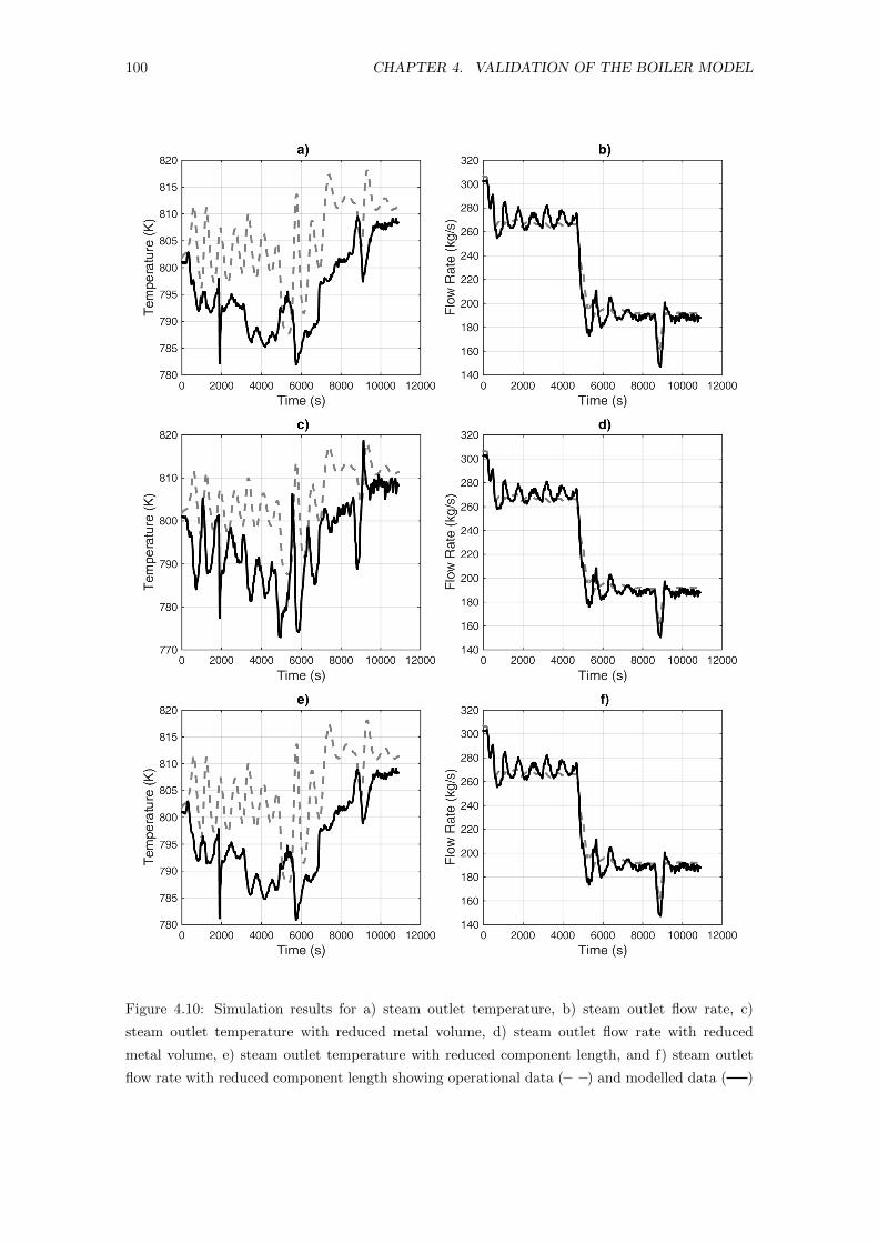
100 CHAPTER 4. VALIDATION OF THE BOILER MODEL
Figure 4.10: Simulation results for a) steam outlet temperature, b) steam outlet flow rate, c)
steam outlet temperature with reduced metal volume, d) steam outlet flow rate with reduced
metal volume, e) steam outlet temperature with reduced component length, and f) steam outlet
flow rate with reduced component length showing operational data ( ) and modelled data ( )
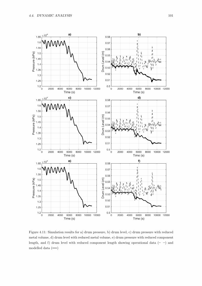
4.4. DYNAMIC ANALYSIS 101
Figure 4.11: Simulation results for a) drum pressure, b) drum level, c) drum pressure with reduced
metal volume, d) drum level with reduced metal volume, e) drum pressure with reduced component
length, and f) drum level with reduced component length showing operational data ( ) and
modelled data ( )
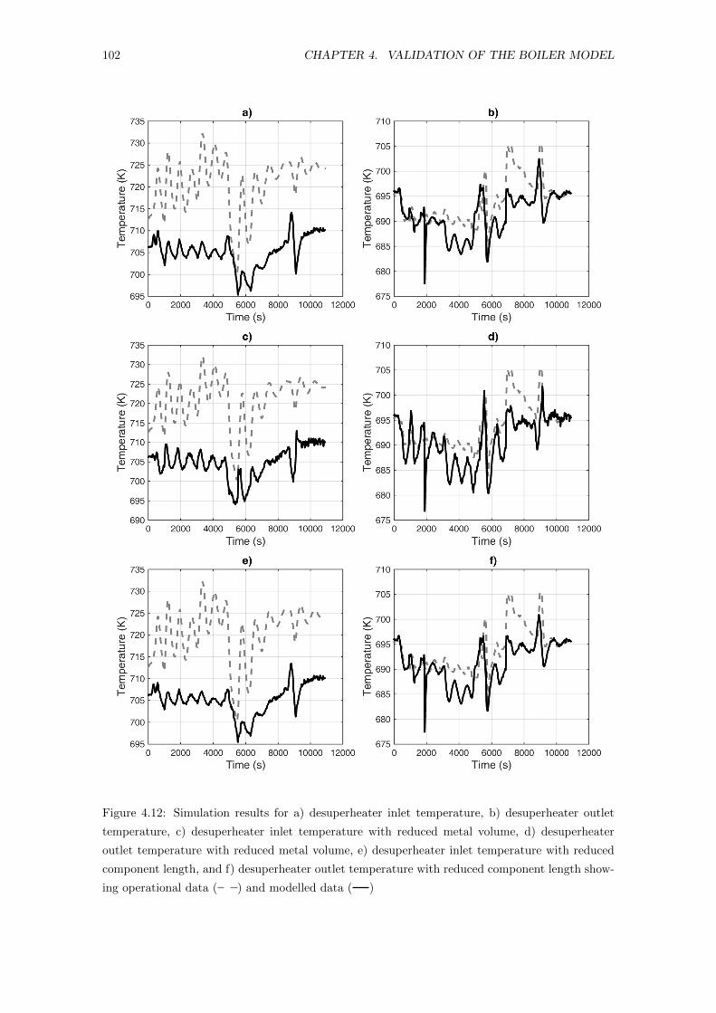
102 CHAPTER 4. VALIDATION OF THE BOILER MODEL
Figure 4.12: Simulation results for a) desuperheater inlet temperature, b) desuperheater outlet
temperature, c) desuperheater inlet temperature with reduced metal volume, d) desuperheater
outlet temperature with reduced metal volume, e) desuperheater inlet temperature with reduced
component length, and f) desuperheater outlet temperature with reduced component length show-
ing operational data ( ) and modelled data ( )
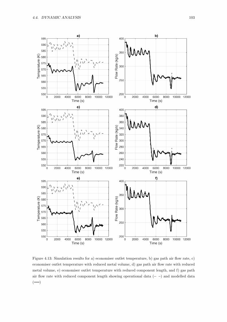
4.4. DYNAMIC ANALYSIS 103
Figure 4.13: Simulation results for a) economiser outlet temperature, b) gas path air flow rate, c)
economiser outlet temperature with reduced metal volume, d) gas path air flow rate with reduced
metal volume, e) economiser outlet temperature with reduced component length, and f) gas path
air flow rate with reduced component length showing operational data ( ) and modelled data
( )
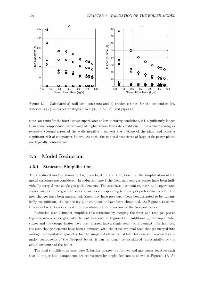
104 CHAPTER 4. VALIDATION OF THE BOILER MODEL
Figure 4.14: Calculated a) wall time constants and b) residence times for the economiser (◦),waterwalls (×), superheater stages 1 to 4 (+, �, B , C), and pipes (�)
time constants for the fourth stage superheater at low operating conditions, it is significantly longer
than some components, particularly at higher steam flow rate conditions. This is unsurprising as
excessive thermal stress of the walls negatively impacts the lifetime of the plant and poses a
significant risk of component failure. As such, the imposed transients of large scale power plants
are typically conservative.
4.5 Model Reduction
4.5.1 Structure Simplification
Three reduced models, shown in Figures 4.15, 4.16, and 4.17, based on the simplification of the
model structure are considered. In reduction case 1 the front and rear gas passes have been indi-
vidually merged into single gas path elements. The associated economiser, riser, and superheater
stages have been merged into single elements corresponding to these gas path elements while the
area changes have been maintained. Since they have previously been demonstrated to be dynam-
ically insignificant, the connecting pipe components have been eliminated. As Figure 4.15 shows
this model reduction case is still representative of the structure of the Newport boiler.
Reduction case 2 further simplifies this structure by merging the front and rear gas passes
together into a single gas path element as shown in Figure 4.16. Additionally, the superheater
stages and the desuperheater have been merged into a single steam path element. Furthermore,
the area change elements have been eliminated with the cross-sectional area changes merged into
average representative geometry for the simplified elements. While this case still represents the
major components of the Newport boiler, it can no longer be considered representative of the
actual structure of the boiler.
The final simplification case, case 3, further merges the furnace and gas passes together such
that all major fluid components are represented by single elements as shown in Figure 4.17. As
4.5. MODEL REDUCTION 105
with the previous case this model structure contains the major components of the boiler but does
not reflect the actual layout of these components. Since it is desirable to ensure that the drum
level can be modelled, this is the simplest model structure that can be considered.
As part of the significant altering of the model structure between the first and second reduction
cases, it is of course necessary to re-optimise the heat transfer coefficients and pressure drop
parameters. This follows the same process as presented previously and as such is not considered
further. The comparison of the simulation results of these simplified models with the operational
data are shown in Figures 4.18 and 4.19 for relevant steam path variables. It can be seen that the
simplified models generally achieve comparable results to the higher order model seen in Figures
4.10 and 4.11. Hence, it can be seen that it is possible to represent a complex and large scale boiler
by a relatively simple model structure with little loss in model fidelity.
4.5.2 Model Order Reduction
The analysis in Section 4.4.1 suggests that the fluid path and wall dynamics could reasonably
be treated as quasi-steady with little loss in model fidelity. However, as indicated previously it is
desirable to ensure the drum level is adequately modelled, which requires that the remaining steam
drum states not be treated as quasi-steady. The further reduction of the model will be considered
in two sequential parts. The first will eliminate the gas path and steam path fluid dynamics, with
exception of the steam drum, by treating these components as quasi-steady. The second part will
further extend this to eliminate the wall dynamics by treating the wall temperatures as quasi-
steady. Hence, with the exception of the steam drum, the remainder of the model is evaluated
algebraically.
Since the third simplification case demonstrated good agreement with the higher order model,
this case will be used for assessing the further reduction of the model. Figures 4.20 and 4.21 show a
comparison between the partially quasi-steady models and the operational data. From these results
it can be seen that the partially quasi-steady models are able to achieve comparable behaviour to
the higher order model seen in Figures 4.10 and 4.11. In the case of the steam outlet temperature
the quasi-steady models actually shows a greater resemblance to the shape of the operational data.
Differences are observed in the drum level with the quasi-steady models demonstrating steadier
behaviour compared to the higher order model. This behaviour is due most significantly to the
enforced quasi-steadiness of the surrounding fluid components reducing the error in conservation
of mass of the drum liquid phase during transients. While this results in the quasi-steady models
demonstrating better agreement with the drum level data this is actually demonstrative of the
sensitivity of the drum level model to this error in mass conservation.
Hence, it has been demonstrated that it is possible to both simplify the structure of the model
and reduce the model to the following four states describing the steam drum behaviour with little
loss in model fidelity:
1. udrum,l,in, the drum liquid inlet velocity,
2. udrum,tp,in, the drum two-phase inlet velocity,
3. ρl,drum, the drum liquid density,
4. ml,drum, the drum liquid mass.
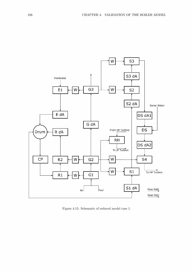
106 CHAPTER 4. VALIDATION OF THE BOILER MODEL
Figure 4.15: Schematic of reduced model case 1.
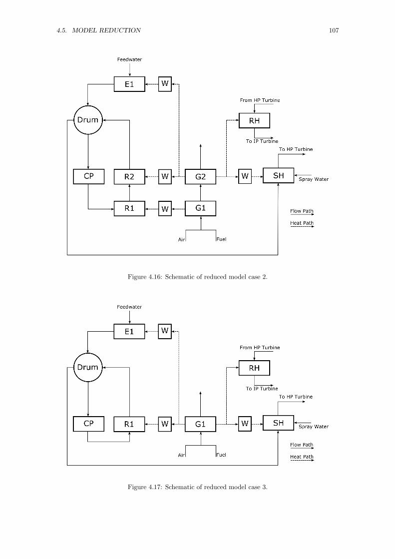
4.5. MODEL REDUCTION 107
Figure 4.16: Schematic of reduced model case 2.
Figure 4.17: Schematic of reduced model case 3.
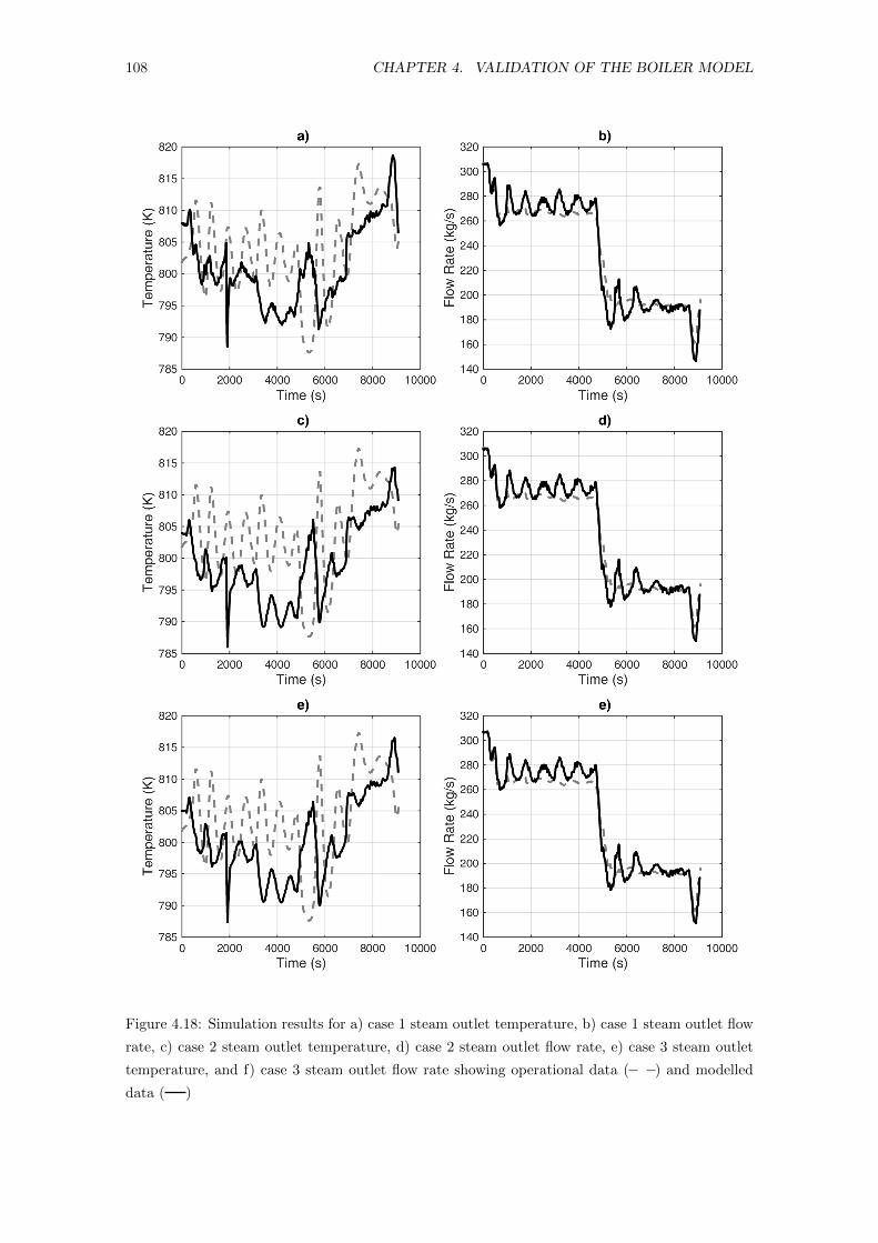
108 CHAPTER 4. VALIDATION OF THE BOILER MODEL
Figure 4.18: Simulation results for a) case 1 steam outlet temperature, b) case 1 steam outlet flow
rate, c) case 2 steam outlet temperature, d) case 2 steam outlet flow rate, e) case 3 steam outlet
temperature, and f) case 3 steam outlet flow rate showing operational data ( ) and modelled
data ( )
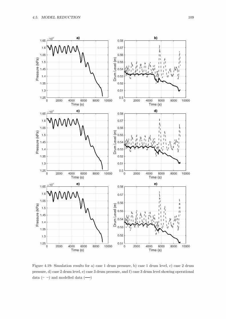
4.5. MODEL REDUCTION 109
Figure 4.19: Simulation results for a) case 1 drum pressure, b) case 1 drum level, c) case 2 drum
pressure, d) case 2 drum level, e) case 3 drum pressure, and f) case 3 drum level showing operational
data ( ) and modelled data ( )
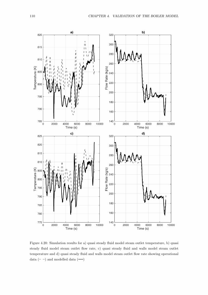
110 CHAPTER 4. VALIDATION OF THE BOILER MODEL
Figure 4.20: Simulation results for a) quasi steady fluid model steam outlet temperature, b) quasi
steady fluid model steam outlet flow rate, c) quasi steady fluid and walls model steam outlet
temperature and d) quasi steady fluid and walls model steam outlet flow rate showing operational
data ( ) and modelled data ( )
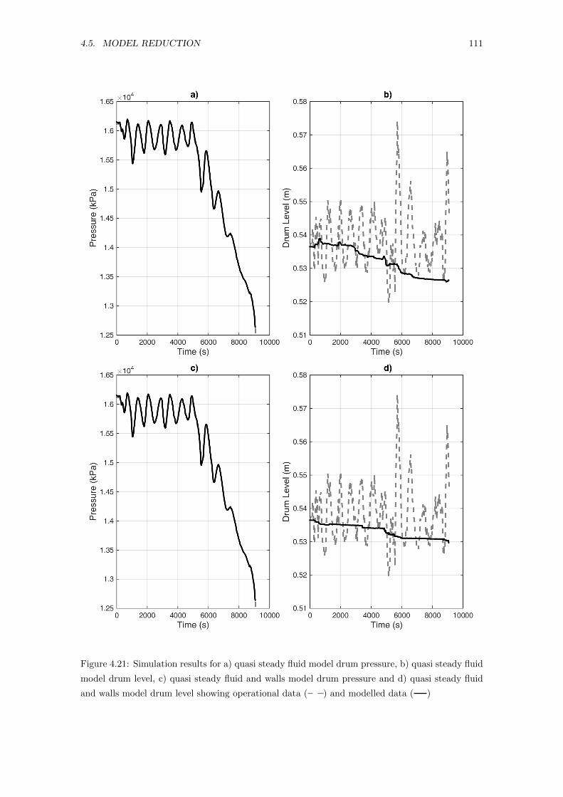
4.5. MODEL REDUCTION 111
Figure 4.21: Simulation results for a) quasi steady fluid model drum pressure, b) quasi steady fluid
model drum level, c) quasi steady fluid and walls model drum pressure and d) quasi steady fluid
and walls model drum level showing operational data ( ) and modelled data ( )
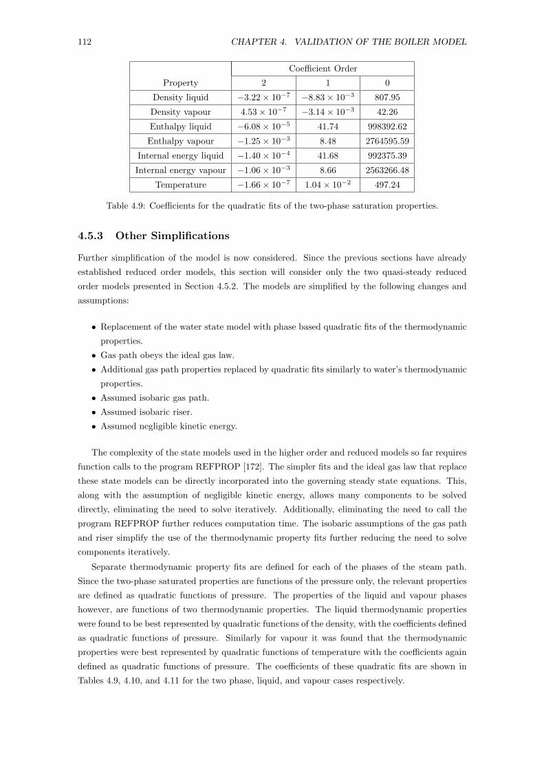
112 CHAPTER 4. VALIDATION OF THE BOILER MODEL
Coefficient Order
Property 2 1 0
Density liquid −3.22× 10⁻⁷ −8.83× 10⁻³ 807.95
Density vapour 4.53× 10⁻⁷ −3.14× 10⁻³ 42.26
Enthalpy liquid −6.08× 10⁻⁵ 41.74 998392.62
Enthalpy vapour −1.25× 10⁻³ 8.48 2764595.59
Internal energy liquid −1.40× 10⁻⁴ 41.68 992375.39
Internal energy vapour −1.06× 10⁻³ 8.66 2563266.48
Temperature −1.66× 10⁻⁷ 1.04× 10⁻² 497.24
Table 4.9: Coefficients for the quadratic fits of the two-phase saturation properties.
4.5.3 Other Simplifications
Further simplification of the model is now considered. Since the previous sections have already
established reduced order models, this section will consider only the two quasi-steady reduced
order models presented in Section 4.5.2. The models are simplified by the following changes and
assumptions:
• Replacement of the water state model with phase based quadratic fits of the thermodynamic
properties.
• Gas path obeys the ideal gas law.
• Additional gas path properties replaced by quadratic fits similarly to water’s thermodynamic
properties.
• Assumed isobaric gas path.
• Assumed isobaric riser.
• Assumed negligible kinetic energy.
The complexity of the state models used in the higher order and reduced models so far requires
function calls to the program REFPROP [172]. The simpler fits and the ideal gas law that replace
these state models can be directly incorporated into the governing steady state equations. This,
along with the assumption of negligible kinetic energy, allows many components to be solved
directly, eliminating the need to solve iteratively. Additionally, eliminating the need to call the
program REFPROP further reduces computation time. The isobaric assumptions of the gas path
and riser simplify the use of the thermodynamic property fits further reducing the need to solve
components iteratively.
Separate thermodynamic property fits are defined for each of the phases of the steam path.
Since the two-phase saturated properties are functions of the pressure only, the relevant properties
are defined as quadratic functions of pressure. The properties of the liquid and vapour phases
however, are functions of two thermodynamic properties. The liquid thermodynamic properties
were found to be best represented by quadratic functions of the density, with the coefficients defined
as quadratic functions of pressure. Similarly for vapour it was found that the thermodynamic
properties were best represented by quadratic functions of temperature with the coefficients again
defined as quadratic functions of pressure. The coefficients of these quadratic fits are shown in
Tables 4.9, 4.10, and 4.11 for the two phase, liquid, and vapour cases respectively.
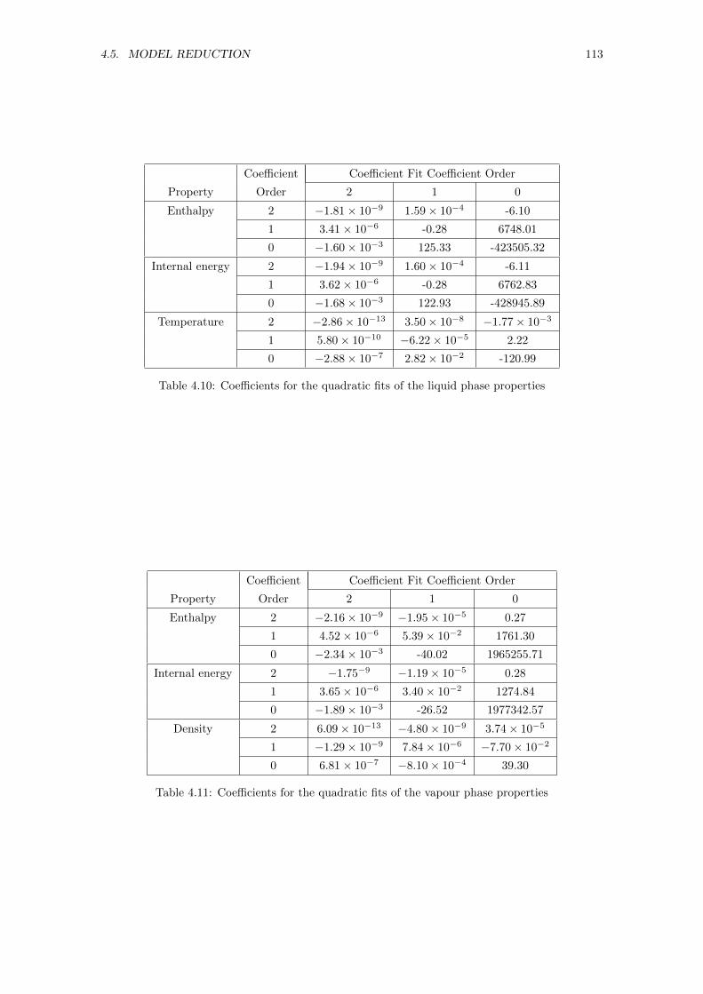
4.5. MODEL REDUCTION 113
Coefficient Coefficient Fit Coefficient Order
Property Order 2 1 0
Enthalpy 2 −1.81× 10⁻⁹ 1.59× 10⁻⁴ -6.10
1 3.41× 10⁻⁶ -0.28 6748.01
0 −1.60× 10⁻³ 125.33 -423505.32
Internal energy 2 −1.94× 10⁻⁹ 1.60× 10⁻⁴ -6.11
1 3.62× 10⁻⁶ -0.28 6762.83
0 −1.68× 10⁻³ 122.93 -428945.89
Temperature 2 −2.86× 10⁻¹³ 3.50× 10⁻⁸ −1.77× 10⁻³
1 5.80× 10⁻¹⁰ −6.22× 10⁻⁵ 2.22
0 −2.88× 10⁻⁷ 2.82× 10⁻² -120.99
Table 4.10: Coefficients for the quadratic fits of the liquid phase properties
Coefficient Coefficient Fit Coefficient Order
Property Order 2 1 0
Enthalpy 2 −2.16× 10⁻⁹ −1.95× 10⁻⁵ 0.27
1 4.52× 10⁻⁶ 5.39× 10⁻² 1761.30
0 −2.34× 10⁻³ -40.02 1965255.71
Internal energy 2 −1.75−9 −1.19× 10⁻⁵ 0.28
1 3.65× 10⁻⁶ 3.40× 10⁻² 1274.84
0 −1.89× 10⁻³ -26.52 1977342.57
Density 2 6.09× 10⁻¹³ −4.80× 10⁻⁹ 3.74× 10⁻⁵
1 −1.29× 10⁻⁹ 7.84× 10⁻⁶ −7.70× 10⁻²
0 6.81× 10⁻⁷ −8.10× 10⁻⁴ 39.30
Table 4.11: Coefficients for the quadratic fits of the vapour phase properties
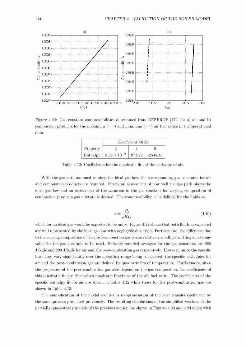
114 CHAPTER 4. VALIDATION OF THE BOILER MODEL
Figure 4.22: Gas constant compressibilities determined from REFPROP [172] for a) air and b)
combustion products for the maximum ( ) and minimum ( ) air fuel ratios in the operational
data.
Coefficient Order
Property 2 1 0
Enthalpy 8.58× 10⁻² 971.22 -2545.15
Table 4.12: Coefficients for the quadratic fits of the enthalpy of air.
With the gas path assumed to obey the ideal gas law, the corresponding gas constants for air
and combustion products are required. Firstly an assessment of how well the gas path obeys the
ideal gas law and an assessment of the variation in the gas constant for varying composition of
combustion products gas mixture is desired. The compressibility, z, is defined for the fluids as
z =PsρRTs
(4.10)
which for an ideal gas would be expected to be unity. Figure 4.22 shows that both fluids as expected
are well represented by the ideal gas law with negligible deviation. Furthermore, the difference due
to the varying composition of the post-combustion gas is also relatively small, permitting an average
value for the gas constant to be used. Suitable rounded averages for the gas constants are 288
J/kgK and 299 J/kgK for air and the post-combustion gas respectively. However, since the specific
heat does vary significantly over the operating range being considered, the specific enthalpies for
air and the post-combustion gas are defined by quadratic fits of temperature. Furthermore, since
the properties of the post-combustion gas also depend on the gas composition, the coefficients of
this quadratic fit are themselves quadratic functions of the air fuel ratio. The coefficients of the
specific enthalpy fit for air are shown in Table 4.12 while those for the post-combustion gas are
shown in Table 4.13.
The simplification of the model required a re-optimisation of the heat transfer coefficient by
the same process presented previously. The resulting simulations of the simplified versions of the
partially quasi-steady models of the previous section are shown in Figures 4.23 and 4.24 along with
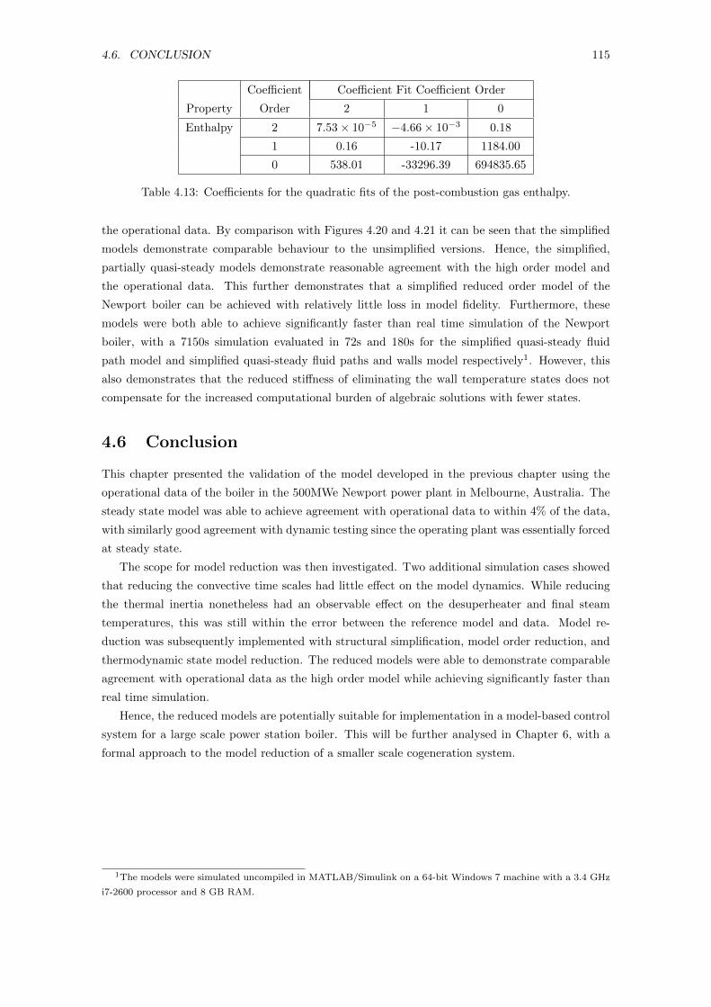
4.6. CONCLUSION 115
Coefficient Coefficient Fit Coefficient Order
Property Order 2 1 0
Enthalpy 2 7.53× 10⁻⁵ −4.66× 10⁻³ 0.18
1 0.16 -10.17 1184.00
0 538.01 -33296.39 694835.65
Table 4.13: Coefficients for the quadratic fits of the post-combustion gas enthalpy.
the operational data. By comparison with Figures 4.20 and 4.21 it can be seen that the simplified
models demonstrate comparable behaviour to the unsimplified versions. Hence, the simplified,
partially quasi-steady models demonstrate reasonable agreement with the high order model and
the operational data. This further demonstrates that a simplified reduced order model of the
Newport boiler can be achieved with relatively little loss in model fidelity. Furthermore, these
models were both able to achieve significantly faster than real time simulation of the Newport
boiler, with a 7150s simulation evaluated in 72s and 180s for the simplified quasi-steady fluid
path model and simplified quasi-steady fluid paths and walls model respectively1. However, this
also demonstrates that the reduced stiffness of eliminating the wall temperature states does not
compensate for the increased computational burden of algebraic solutions with fewer states.
4.6 Conclusion
This chapter presented the validation of the model developed in the previous chapter using the
operational data of the boiler in the 500MWe Newport power plant in Melbourne, Australia. The
steady state model was able to achieve agreement with operational data to within 4% of the data,
with similarly good agreement with dynamic testing since the operating plant was essentially forced
at steady state.
The scope for model reduction was then investigated. Two additional simulation cases showed
that reducing the convective time scales had little effect on the model dynamics. While reducing
the thermal inertia nonetheless had an observable effect on the desuperheater and final steam
temperatures, this was still within the error between the reference model and data. Model re-
duction was subsequently implemented with structural simplification, model order reduction, and
thermodynamic state model reduction. The reduced models were able to demonstrate comparable
agreement with operational data as the high order model while achieving significantly faster than
real time simulation.
Hence, the reduced models are potentially suitable for implementation in a model-based control
system for a large scale power station boiler. This will be further analysed in Chapter 6, with a
formal approach to the model reduction of a smaller scale cogeneration system.
1The models were simulated uncompiled in MATLAB/Simulink on a 64-bit Windows 7 machine with a 3.4 GHz
i7-2600 processor and 8 GB RAM.
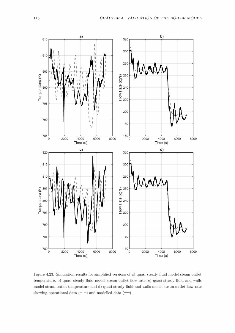
116 CHAPTER 4. VALIDATION OF THE BOILER MODEL
Figure 4.23: Simulation results for simplified versions of a) quasi steady fluid model steam outlet
temperature, b) quasi steady fluid model steam outlet flow rate, c) quasi steady fluid and walls
model steam outlet temperature and d) quasi steady fluid and walls model steam outlet flow rate
showing operational data ( ) and modelled data ( )
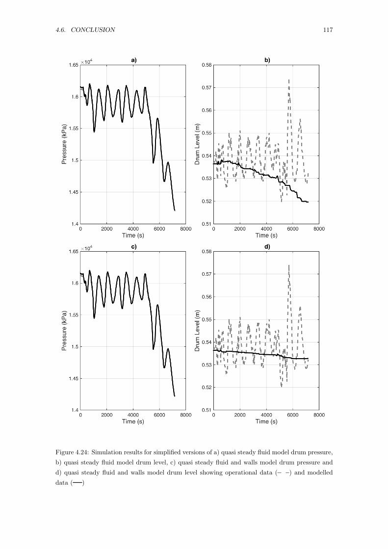
4.6. CONCLUSION 117
Figure 4.24: Simulation results for simplified versions of a) quasi steady fluid model drum pressure,
b) quasi steady fluid model drum level, c) quasi steady fluid and walls model drum pressure and
d) quasi steady fluid and walls model drum level showing operational data ( ) and modelled
data ( )

118 CHAPTER 4. VALIDATION OF THE BOILER MODEL
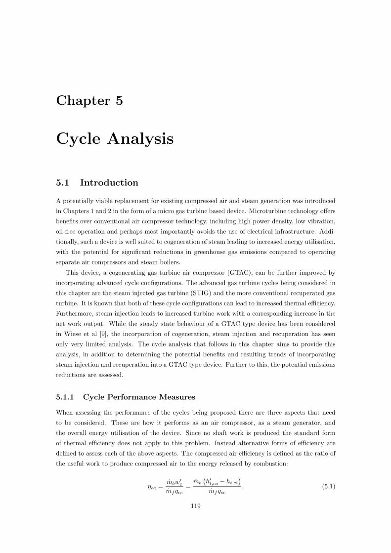
Chapter 5
Cycle Analysis
5.1 Introduction
A potentially viable replacement for existing compressed air and steam generation was introduced
in Chapters 1 and 2 in the form of a micro gas turbine based device. Microturbine technology offers
benefits over conventional air compressor technology, including high power density, low vibration,
oil-free operation and perhaps most importantly avoids the use of electrical infrastructure. Addi-
tionally, such a device is well suited to cogeneration of steam leading to increased energy utilisation,
with the potential for significant reductions in greenhouse gas emissions compared to operating
separate air compressors and steam boilers.
This device, a cogenerating gas turbine air compressor (GTAC), can be further improved by
incorporating advanced cycle configurations. The advanced gas turbine cycles being considered in
this chapter are the steam injected gas turbine (STIG) and the more conventional recuperated gas
turbine. It is known that both of these cycle configurations can lead to increased thermal efficiency.
Furthermore, steam injection leads to increased turbine work with a corresponding increase in the
net work output. While the steady state behaviour of a GTAC type device has been considered
in Wiese et al [9], the incorporation of cogeneration, steam injection and recuperation has seen
only very limited analysis. The cycle analysis that follows in this chapter aims to provide this
analysis, in addition to determining the potential benefits and resulting trends of incorporating
steam injection and recuperation into a GTAC type device. Further to this, the potential emissions
reductions are assessed.
5.1.1 Cycle Performance Measures
When assessing the performance of the cycles being proposed there are three aspects that need
to be considered. These are how it performs as an air compressor, as a steam generator, and
the overall energy utilisation of the device. Since no shaft work is produced the standard form
of thermal efficiency does not apply to this problem. Instead alternative forms of efficiency are
defined to assess each of the above aspects. The compressed air efficiency is defined as the ratio of
the useful work to produce compressed air to the energy released by combustion:
ηca =mbw
′c
mfqcc=mb
(h′t,co − ht,ci
)mfqcc
. (5.1)
119

120 CHAPTER 5. CYCLE ANALYSIS
The useful work is defined as the portion of isentropic work that leads to the delivery pressure and
rate before consideration of irreversible compressor behaviour. The steam efficiency is defined as
the ratio of the energy from the exhaust required to produce the cogenerated steam to the energy
released by combustion:
ηs =ms,cogenqhrsg
mfqcc=ms,cogen (ht,hrsg,o − ht,hrsg,i)
mfqcc. (5.2)
It should be noted that the steam and compressed air efficiencies only consider the production of
steam and compressed air and not the subsequent use of these substances. The analysis presented
in this chapter is concerned only with production as the end use of the two substances will be the
same regardless of production method. As such, improvements in the efficiency of producing the
compressed air and steam will correspond to improvements in the overall system that the device
is part of.
The overall efficiency, which assesses useful energy utilisation, is defined as the ratio of the
useful energy out in the form of compressed air and steam to the energy released by combustion:
ηo =mbw
′c + ms,cogenqhrsg
mfqcc= ηca + ηs. (5.3)
As a result of this definition the overall efficiency equates to the sum of the compressed air and
steam efficiencies.
5.1.2 Proposed Cycles
Four cycles based on variations of the basic GTAC cycle are being analysed to assess (both quali-
tatively and quantitatively) the potential benefits of combining steam generation with compressed
air production in a microturbine based device incorporating advanced cycle configurations. The
cycles being considered, which are described below, are the basic GTAC with cogeneration, the
recuperated GTAC, the STIGTAC and the recuperated STIGTAC.
The first cycle configuration analysed, the basic GTAC with cogeneration, is shown in Figure
5.1 A). This is the GTAC with a HRSG attached using the high temperature exhaust to generate
steam, and represents the simplest cogeneration device considered. This makes it the most appro-
priate base comparison case to consider what improvements are possible with more advanced cycle
configurations or alternative waste heat recovery methods.
Conventional heat recovery in low pressure ratio devices is achieved through recuperation,
shown in Figure 5.1 B). The high temperature exhaust is used to preheat air entering the combus-
tion chamber using a heat exchanger (the recuperator). Hence, the required heat from combustion
is reduced, increasing the compressed air efficiency. While not a form of cogeneration it is a con-
ventional waste heat recovery method making it a useful comparison case. In particular, being
more direct in terms of the energy transfer may lead to superior improvements at low pressure
ratios compared to the steam injected cycle variations. In fact, it is known that the peak thermal
efficiency of a recuperated gas turbine is at a pressure ratio lower than the simple cycle gas turbine
as the heat transfer in the recuperator decreases with decreasing exhaust temperature [51].
The cycle configuration of most interest is the Steam Injected Gas Turbine Air Compressor
(STIGTAC), shown in Figure 5.1 C). In the STIGTAC cycle a portion of the steam generated in
the HRSG is injected into the combustion chamber to augment the cycle. Given the literature on
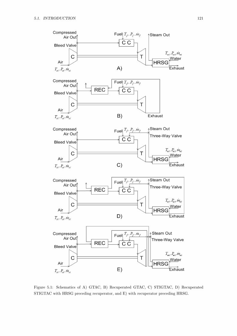
5.1. INTRODUCTION 121
Figure 5.1: Schematics of A) GTAC, B) Recuperated GTAC, C) STIGTAC, D) Recuperated
STIGTAC with HRSG preceding recuperator, and E) with recuperator preceding HRSG.
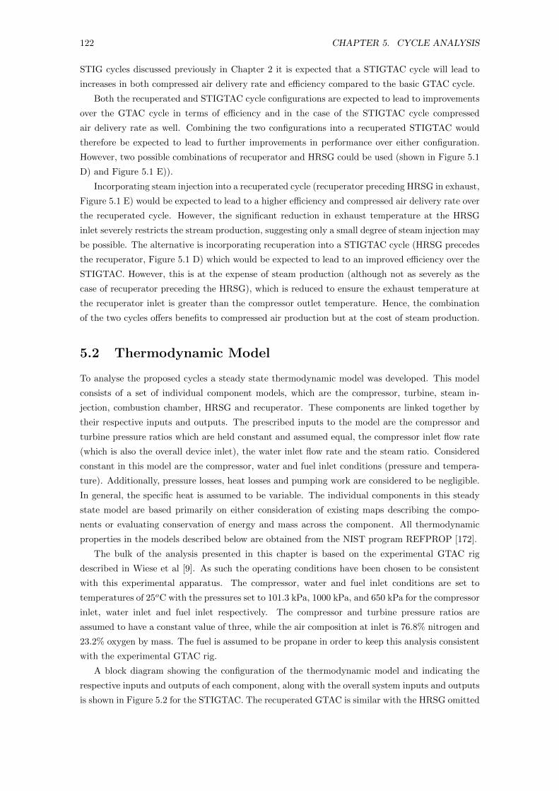
122 CHAPTER 5. CYCLE ANALYSIS
STIG cycles discussed previously in Chapter 2 it is expected that a STIGTAC cycle will lead to
increases in both compressed air delivery rate and efficiency compared to the basic GTAC cycle.
Both the recuperated and STIGTAC cycle configurations are expected to lead to improvements
over the GTAC cycle in terms of efficiency and in the case of the STIGTAC cycle compressed
air delivery rate as well. Combining the two configurations into a recuperated STIGTAC would
therefore be expected to lead to further improvements in performance over either configuration.
However, two possible combinations of recuperator and HRSG could be used (shown in Figure 5.1
D) and Figure 5.1 E)).
Incorporating steam injection into a recuperated cycle (recuperator preceding HRSG in exhaust,
Figure 5.1 E) would be expected to lead to a higher efficiency and compressed air delivery rate over
the recuperated cycle. However, the significant reduction in exhaust temperature at the HRSG
inlet severely restricts the stream production, suggesting only a small degree of steam injection may
be possible. The alternative is incorporating recuperation into a STIGTAC cycle (HRSG precedes
the recuperator, Figure 5.1 D) which would be expected to lead to an improved efficiency over the
STIGTAC. However, this is at the expense of steam production (although not as severely as the
case of recuperator preceding the HRSG), which is reduced to ensure the exhaust temperature at
the recuperator inlet is greater than the compressor outlet temperature. Hence, the combination
of the two cycles offers benefits to compressed air production but at the cost of steam production.
5.2 Thermodynamic Model
To analyse the proposed cycles a steady state thermodynamic model was developed. This model
consists of a set of individual component models, which are the compressor, turbine, steam in-
jection, combustion chamber, HRSG and recuperator. These components are linked together by
their respective inputs and outputs. The prescribed inputs to the model are the compressor and
turbine pressure ratios which are held constant and assumed equal, the compressor inlet flow rate
(which is also the overall device inlet), the water inlet flow rate and the steam ratio. Considered
constant in this model are the compressor, water and fuel inlet conditions (pressure and tempera-
ture). Additionally, pressure losses, heat losses and pumping work are considered to be negligible.
In general, the specific heat is assumed to be variable. The individual components in this steady
state model are based primarily on either consideration of existing maps describing the compo-
nents or evaluating conservation of energy and mass across the component. All thermodynamic
properties in the models described below are obtained from the NIST program REFPROP [172].
The bulk of the analysis presented in this chapter is based on the experimental GTAC rig
described in Wiese et al [9]. As such the operating conditions have been chosen to be consistent
with this experimental apparatus. The compressor, water and fuel inlet conditions are set to
temperatures of 25oC with the pressures set to 101.3 kPa, 1000 kPa, and 650 kPa for the compressor
inlet, water inlet and fuel inlet respectively. The compressor and turbine pressure ratios are
assumed to have a constant value of three, while the air composition at inlet is 76.8% nitrogen and
23.2% oxygen by mass. The fuel is assumed to be propane in order to keep this analysis consistent
with the experimental GTAC rig.
A block diagram showing the configuration of the thermodynamic model and indicating the
respective inputs and outputs of each component, along with the overall system inputs and outputs
is shown in Figure 5.2 for the STIGTAC. The recuperated GTAC is similar with the HRSG omitted
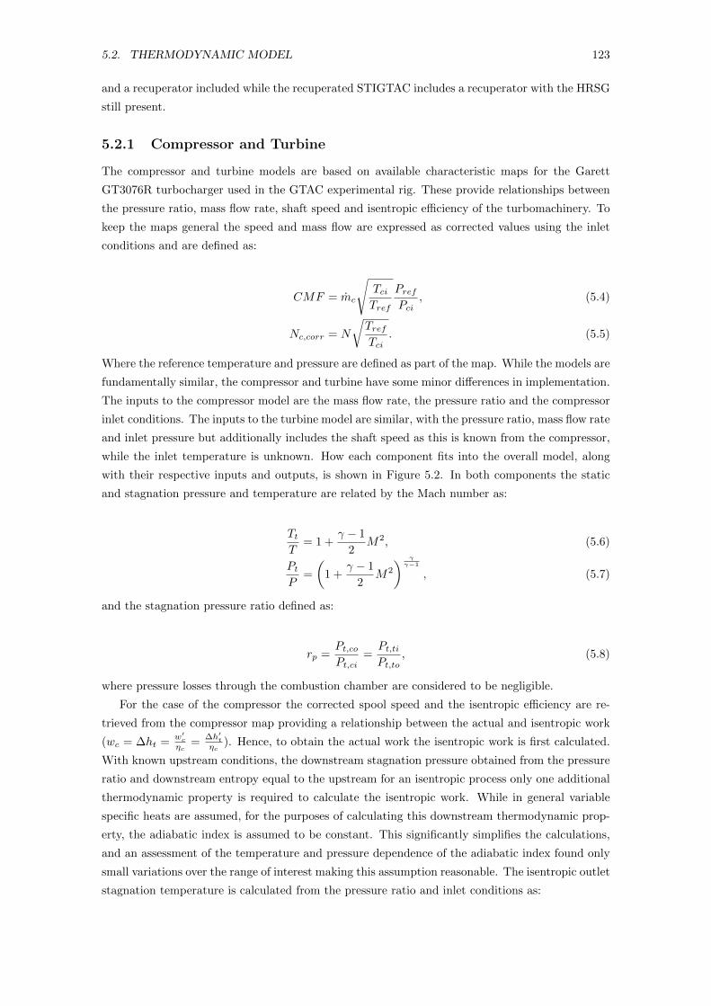
5.2. THERMODYNAMIC MODEL 123
and a recuperator included while the recuperated STIGTAC includes a recuperator with the HRSG
still present.
5.2.1 Compressor and Turbine
The compressor and turbine models are based on available characteristic maps for the Garett
GT3076R turbocharger used in the GTAC experimental rig. These provide relationships between
the pressure ratio, mass flow rate, shaft speed and isentropic efficiency of the turbomachinery. To
keep the maps general the speed and mass flow are expressed as corrected values using the inlet
conditions and are defined as:
CMF = mc
√TciTref
PrefPci
, (5.4)
Nc,corr = N
√TrefTci
. (5.5)
Where the reference temperature and pressure are defined as part of the map. While the models are
fundamentally similar, the compressor and turbine have some minor differences in implementation.
The inputs to the compressor model are the mass flow rate, the pressure ratio and the compressor
inlet conditions. The inputs to the turbine model are similar, with the pressure ratio, mass flow rate
and inlet pressure but additionally includes the shaft speed as this is known from the compressor,
while the inlet temperature is unknown. How each component fits into the overall model, along
with their respective inputs and outputs, is shown in Figure 5.2. In both components the static
and stagnation pressure and temperature are related by the Mach number as:
TtT
= 1 +γ − 1
2M2, (5.6)
PtP
=
(1 +
γ − 1
2M2
) γγ−1
, (5.7)
and the stagnation pressure ratio defined as:
rp =Pt,coPt,ci
=Pt,tiPt,to
, (5.8)
where pressure losses through the combustion chamber are considered to be negligible.
For the case of the compressor the corrected spool speed and the isentropic efficiency are re-
trieved from the compressor map providing a relationship between the actual and isentropic work
(wc = ∆ht =w′cηc
=∆h′tηc
). Hence, to obtain the actual work the isentropic work is first calculated.
With known upstream conditions, the downstream stagnation pressure obtained from the pressure
ratio and downstream entropy equal to the upstream for an isentropic process only one additional
thermodynamic property is required to calculate the isentropic work. While in general variable
specific heats are assumed, for the purposes of calculating this downstream thermodynamic prop-
erty, the adiabatic index is assumed to be constant. This significantly simplifies the calculations,
and an assessment of the temperature and pressure dependence of the adiabatic index found only
small variations over the range of interest making this assumption reasonable. The isentropic outlet
stagnation temperature is calculated from the pressure ratio and inlet conditions as:
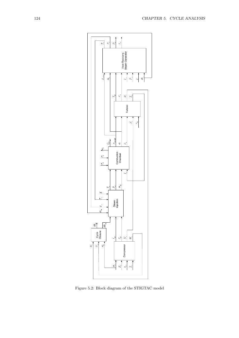
124 CHAPTER 5. CYCLE ANALYSIS
Figure 5.2: Block diagram of the STIGTAC model
5.2. THERMODYNAMIC MODEL 125
Tt,co = Tt,cirγ−1γ
p . (5.9)
The downstream Mach number is subsequently calculated for the isentropic case from:
M =m
APt
√RTtγ
(1 +
γ − 1
2M2
) 12 ( γ+1
γ−1 ). (5.10)
With the Mach number known, the static downstream temperature and pressure can be cal-
culated from (5.6) and (5.7) and subsequently the downstream velocity. Hence, the isentropic
work can be calculated from the stagnation enthalpy difference. The actual compressor work can
subsequently be calculated and the downstream stagnation enthalpy found. The downstream tem-
perature and pressure are subsequently calculated iteratively to match the stagnation enthalpy
with the velocity calculated from the Mach number evaluated using (5.10).
The turbine model is evaluated in much the same manner with some minor differences in the
initial map calculations. The turbine CMF is known to be primarily a function of the pressure
ratio with only a weak dependence on the corrected shaft speed. Hence, from (5.4) the turbine
inlet temperature can be calculated using the CMF and mass flow rate with the corrected speed
calculated from (5.5) allowing the turbine isentropic efficiency to be obtained from the turbine
map. With these known the remainder of the calculations proceed as per the compressor model.
5.2.2 Steam Injection
The steam injection process is modelled using conservation of energy via the enthalpy balance:
maht,co + msht,s = (ma + ms)ht,si = msiht,si. (5.11)
Since pressure losses and heat losses are being neglected steam injection before, after or during
combustion will give the same result. Hence, for this model steam injection is assumed to occur
prior to combustion. The inputs to the model (which can be seen in Figure 5.2) are the air inlet
conditions and mass flow rate, the steam inlet conditions and the steam ratio, which relates the
mass flow rate of steam to the air it is being injected into and is defined as:
S =ms
ma. (5.12)
Since the Mach numbers through this section are relatively low it is reasonable to assume
that the outlet pressure is approximately equal to the air inlet pressure (the compressor outlet
pressure) [186]. Combined with the outlet stagnation enthalpy calculated from (5.11) this allows
two downstream thermodynamic properties (pressure and static enthalpy) to be found allowing
the outlet temperature to be retrieved from REFPROP.
5.2.3 Combustion Chamber
Similarly to steam injection the combustion chamber is modelled using conservation of energy
through the enthalpy balance:
126 CHAPTER 5. CYCLE ANALYSIS
masht,as + mfht,f = (mas + mf )ht,ti = mtht,ti. (5.13)
However, unlike the steam injection process a chemical reaction, in the form of combustion, takes
place (see (5.15)). As such, it is now necessary to take into account the enthalpies of formation
(for steam injection these would cancel on either side of the enthalpy balance) and the stagnation
enthalpy is now defined as:
ht =
(h+
u2
2+ ∆hfo
). (5.14)
As can be seen in Figure 5.2 the inputs to the combustion chamber model are the air-steam
mixture inlet conditions and mass flow rate, the fuel inlet conditions and the turbine inlet temper-
ature (which is from the turbine model). The outputs are the fuel flow rate, exhaust composition
and combustion heat addition.
To retrieve the combustion chamber outlet enthalpy from REFPROP as part of solving (5.13)
the exhaust composition is required. This composition is obtained from consideration of the stoi-
chiometry of combustion of propane with additional steam as shown:
C3H8+a (O2 + 3.76N2)+eH2O → 3CO2 + cH2O + dO2 + 3.76aN2 (5.15)
a =5
φ, (5.16)
c =4 +5S (MO2
+ 3.76MN2)
φMH2O, (5.17)
d =5
φ− 5, (5.18)
e =5S (MO2
+ 3.76MN2)
φMH2O. (5.19)
Where the equivalence ratio, φ, is defined as:
φ =FAR
FARstoich=
mfma(
mfma
)stoich
. (5.20)
With the inlet mass flow rate and steam ratio assumed known the composition becomes a function
of the fuel mass flow rate. Furthermore it can be recalled from the turbine model (Section 5.2.1)
that since the pressure ratio is considered fixed, the turbine inlet temperature is effectively a
function of the the turbine mass flow rate meaning the turbine inlet temperature is also effectively
a function of the fuel flow rate. Hence (5.13) can be solved to obtain the fuel flow rate and
subsequently the turbine mass flow rate. As such the combustion chamber calculations are linked
to the turbine model requiring them to be solved concurrently. This can be seen in Figure 5.2.
5.2.4 Recuperator and HRSG
While a detailed dynamic model for a boiler was developed in Chapter 3 which included steady state
calculations this will not be used here. Instead a simpler approach is used with the recuperator
and HRSG both modelled as counter-flow heat exchangers with known inlet conditions and mass
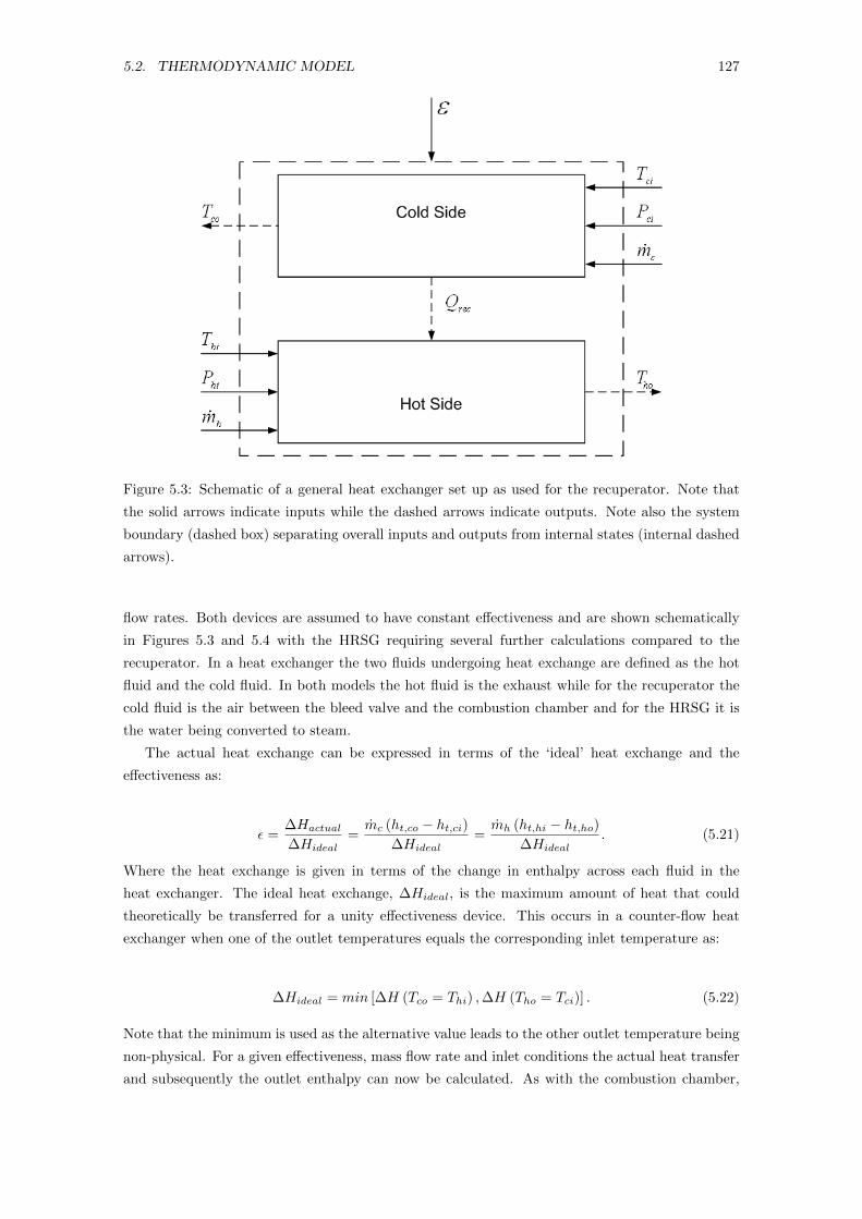
5.2. THERMODYNAMIC MODEL 127
Figure 5.3: Schematic of a general heat exchanger set up as used for the recuperator. Note that
the solid arrows indicate inputs while the dashed arrows indicate outputs. Note also the system
boundary (dashed box) separating overall inputs and outputs from internal states (internal dashed
arrows).
flow rates. Both devices are assumed to have constant effectiveness and are shown schematically
in Figures 5.3 and 5.4 with the HRSG requiring several further calculations compared to the
recuperator. In a heat exchanger the two fluids undergoing heat exchange are defined as the hot
fluid and the cold fluid. In both models the hot fluid is the exhaust while for the recuperator the
cold fluid is the air between the bleed valve and the combustion chamber and for the HRSG it is
the water being converted to steam.
The actual heat exchange can be expressed in terms of the ‘ideal’ heat exchange and the
effectiveness as:
ε =∆Hactual
∆Hideal=mc (ht,co − ht,ci)
∆Hideal=mh (ht,hi − ht,ho)
∆Hideal. (5.21)
Where the heat exchange is given in terms of the change in enthalpy across each fluid in the
heat exchanger. The ideal heat exchange, ∆Hideal, is the maximum amount of heat that could
theoretically be transferred for a unity effectiveness device. This occurs in a counter-flow heat
exchanger when one of the outlet temperatures equals the corresponding inlet temperature as:
∆Hideal = min [∆H (Tco = Thi) ,∆H (Tho = Tci)] . (5.22)
Note that the minimum is used as the alternative value leads to the other outlet temperature being
non-physical. For a given effectiveness, mass flow rate and inlet conditions the actual heat transfer
and subsequently the outlet enthalpy can now be calculated. As with the combustion chamber,
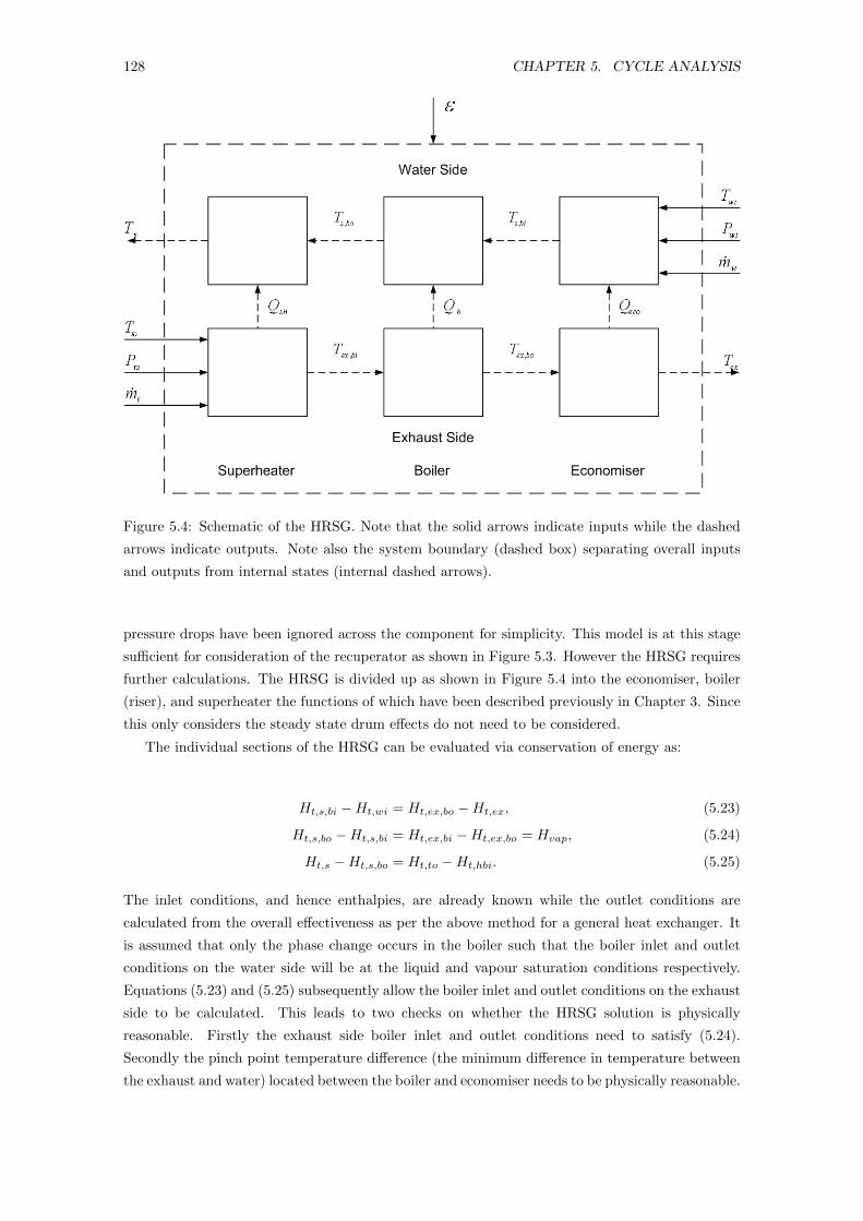
128 CHAPTER 5. CYCLE ANALYSIS
Figure 5.4: Schematic of the HRSG. Note that the solid arrows indicate inputs while the dashed
arrows indicate outputs. Note also the system boundary (dashed box) separating overall inputs
and outputs from internal states (internal dashed arrows).
pressure drops have been ignored across the component for simplicity. This model is at this stage
sufficient for consideration of the recuperator as shown in Figure 5.3. However the HRSG requires
further calculations. The HRSG is divided up as shown in Figure 5.4 into the economiser, boiler
(riser), and superheater the functions of which have been described previously in Chapter 3. Since
this only considers the steady state drum effects do not need to be considered.
The individual sections of the HRSG can be evaluated via conservation of energy as:
Ht,s,bi −Ht,wi = Ht,ex,bo −Ht,ex, (5.23)
Ht,s,bo −Ht,s,bi = Ht,ex,bi −Ht,ex,bo = Hvap, (5.24)
Ht,s −Ht,s,bo = Ht,to −Ht,hbi. (5.25)
The inlet conditions, and hence enthalpies, are already known while the outlet conditions are
calculated from the overall effectiveness as per the above method for a general heat exchanger. It
is assumed that only the phase change occurs in the boiler such that the boiler inlet and outlet
conditions on the water side will be at the liquid and vapour saturation conditions respectively.
Equations (5.23) and (5.25) subsequently allow the boiler inlet and outlet conditions on the exhaust
side to be calculated. This leads to two checks on whether the HRSG solution is physically
reasonable. Firstly the exhaust side boiler inlet and outlet conditions need to satisfy (5.24).
Secondly the pinch point temperature difference (the minimum difference in temperature between
the exhaust and water) located between the boiler and economiser needs to be physically reasonable.
5.2. THERMODYNAMIC MODEL 129
In practice a pinch point of 10◦C is the standard design assumption [187]. The physicality of the
‘hot end’ temperature difference, which is at the exhaust inlet end, can also be checked and is in
practice limited to about 20◦C [187]. Given the range of operating conditions considered, these
parameters have been allowed to float as long they remain physically reasonable.
While the use of an effectiveness is applicable to an air to air heat exchanger, such as a recu-
perator, it is not traditionally applied to a device like a HRSG where a phase change occurs. In
practice the above given pinch point and hot end assumptions are what is used for design purposes.
It is generally not possible (theoretically or other wise) for an outlet temperature of a HRSG to
equal the corresponding inlet temperature. The actual temperature profiles depend on the specific
heats and respective mass flow rates of steam and water. The higher heat transfer coefficients for
liquid generally lead to the pinch point being the closer approach over the hot end [187]. As such
even for the non-physical case of a pinch point temperature difference of zero the exhaust inlet
temperature will still be greater than the steam outlet temperature. However, with consideration of
maintaining the actual pinch point and hot end temperature differences within reasonable physical
bounds the use of an effectiveness is a valid way of defining the HRSG.
5.2.5 Cycle Closure
Each of the components within the model have now been defined but the overall system is incom-
plete. The combustion chamber and subsequent components assumed a known mass flow rate of
air. However, this flow rate and that of the bled air are unknown and their calculation forms the
final closure of the cycle. To solve this it can be recognised that the GTAC does not produce
external shaft work, hence, the turbine and compressor have equal work:
mcwc = mtwt. (5.26)
Furthermore from conservation of mass it can be recognised that:
mc = mb + ma. (5.27)
This leads to sufficient equations for all variables to solved for iteratively. For the basic GTAC
(i.e. no steam injection or recuperation) this is sufficient to completely resolve the operating point.
However for either steam injection or recuperation, knowledge of the exhaust is required for the
HRSG and recuperator models. This requires an additional level of iteration to solve for either the
steam temperature at injection or the exhaust temperature entering the recuperator. For the case of
a recuperated STIGTAC both are required, leading to a further additional level of iteration. Hence,
the operating conditions for a GTAC, STIGTAC, recuperated GTAC, or recuperated STIGTAC
cycle can be completely defined.
5.2.6 First Law Balance
Unfortunately the nature of cycle analysis is that it cannot be validated in a rigourous sense without
comparison to experimental data, however it can be assessed to ensure it adequately obeys the
laws of thermodynamics. This determines if the model developed and implemented is based on
130 CHAPTER 5. CYCLE ANALYSIS
Table 5.1: Results of selected points for enthalpy balance over STIGTAC cycle. The enthalpy
difference is expressed both in absolute terms and as a percentage of the fuel heat release.
S mc mw Hin Hout Hdiff
(-) (kg/s) (kg/s) (kW) (kW) (kW) (%)
0.05 0.345 0.0138 -226.57 -226.91 0.34 0.22
0.05 0.345 0.0438 -702.53 -702.87 0.34 0.22
0.1 0.365 0.0247 -400.60 -401.18 0.58 0.31
0.1 0.365 0.0497 -797.23 -797.82 0.59 0.31
0.2 0.39 0.0404 -652.56 -653.41 0.85 0.35
0.2 0.39 0.0604 -969.87 -970.74 0.87 0.36
0.3 0.4 0.0558 -896.76 -897.72 0.95 0.39
0.3 0.4 0.0608 -976.09 -977.05 0.96 0.39
sound physics and achieves accurate cycle closure. To assess this accuracy the first law balance for
the overall device is evaluated as
Ht,ci +Ht,f +Ht,wi = Ht,ex +Ht,b +Ht,so. (5.28)
Table 5.1 shows the results of the enthalpy balance for a selection of operating conditions. The
discrepancy between the enthalpy in and the enthalpy out can be seen to be small relative to the
absolute enthalpy terms and with respect to the total heat release from the fuel. Therefore the
model demonstrates a reasonable satisfaction of conservation of energy and accurate cycle closure.
5.3 Cycle Analysis Results
5.3.1 Steam Injection
Three significant trends for increasing steam ratio are revealed by Figures 5.5 and 5.6. These are
increased bleed flow, decreased cogenerated steam supply, and a reduced operating range. The
two primary factors leading to the increased bleed flow are the addition of mass from the injected
steam, and an increase in the compressor mass flow rate. Since the turbine CMF is effectively a
function of the pressure ratio, which is constant, it will be approximately constant. Hence, for a
given turbine inlet temperature and pressure (5.4) shows that the turbine mass flow rate is fixed.
With no pressure losses and low Mach numbers the turbine inlet pressure is approximately constant
for all operating points. The turbine inlet temperature is limited by a maximum allowable value
(1200K), restricting the operating range of the turbine to the same maximum mass flow rate for
all steam ratios, which manifests in Figures 5.5 to 5.8 as the limit on maximum compressed air
production. Therefore, the injected steam substitutes for a portion of the air that would otherwise
be passing through the turbine, leading to an increase in bleed flow.
This does not, however, account for the entire increase in bleed flow. The remainder is a result
of the increased compressor flow rate. Since the compressor inlet conditions (and by extension the
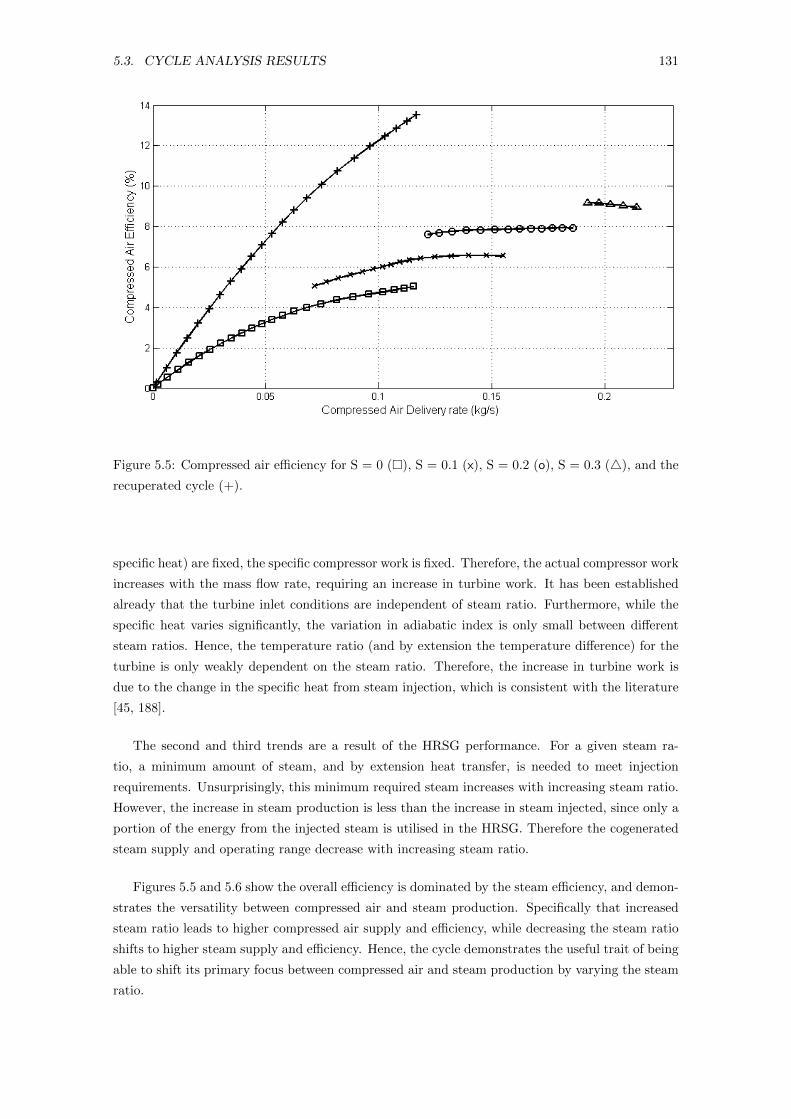
5.3. CYCLE ANALYSIS RESULTS 131
Figure 5.5: Compressed air efficiency for S = 0 (�), S = 0.1 (x), S = 0.2 (o), S = 0.3 (4), and the
recuperated cycle (+).
specific heat) are fixed, the specific compressor work is fixed. Therefore, the actual compressor work
increases with the mass flow rate, requiring an increase in turbine work. It has been established
already that the turbine inlet conditions are independent of steam ratio. Furthermore, while the
specific heat varies significantly, the variation in adiabatic index is only small between different
steam ratios. Hence, the temperature ratio (and by extension the temperature difference) for the
turbine is only weakly dependent on the steam ratio. Therefore, the increase in turbine work is
due to the change in the specific heat from steam injection, which is consistent with the literature
[45, 188].
The second and third trends are a result of the HRSG performance. For a given steam ra-
tio, a minimum amount of steam, and by extension heat transfer, is needed to meet injection
requirements. Unsurprisingly, this minimum required steam increases with increasing steam ratio.
However, the increase in steam production is less than the increase in steam injected, since only a
portion of the energy from the injected steam is utilised in the HRSG. Therefore the cogenerated
steam supply and operating range decrease with increasing steam ratio.
Figures 5.5 and 5.6 show the overall efficiency is dominated by the steam efficiency, and demon-
strates the versatility between compressed air and steam production. Specifically that increased
steam ratio leads to higher compressed air supply and efficiency, while decreasing the steam ratio
shifts to higher steam supply and efficiency. Hence, the cycle demonstrates the useful trait of being
able to shift its primary focus between compressed air and steam production by varying the steam
ratio.
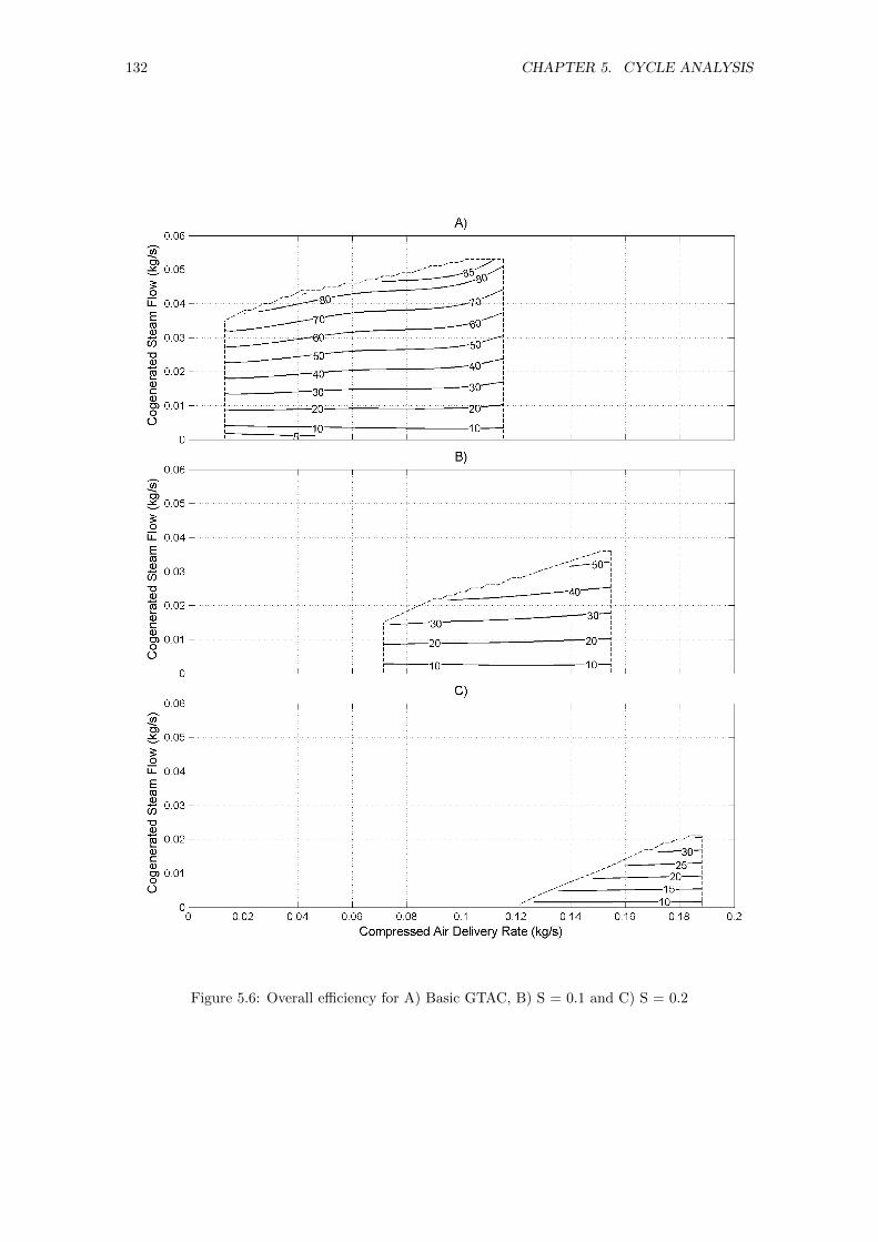
132 CHAPTER 5. CYCLE ANALYSIS
Figure 5.6: Overall efficiency for A) Basic GTAC, B) S = 0.1 and C) S = 0.2
5.4. GREENHOUSE GAS EMISSIONS ANALYSIS 133
5.3.2 Recuperation
The analysis so far has shown that significant increases in compressed air efficiency and delivery
rate are possible using steam injection. However, it can be seen from Figure 5.5 that the com-
pressed air efficiency of the recuperated GTAC is significantly higher than that achieved through
steam injection. This is unsurprising given that the performance increase from steam injection
is limited by turbine performance and the limited energy utilisation of the injected steam. The
recuperator, however, utilises more of the energy extracted from the exhaust, and is not dependent
on turbine performance as the same operating point is effectively being maintained. Furthermore,
the low pressure ratio favours recuperation due to the higher temperature difference between the
compressor and turbine outlets. The compressed air delivery rate is unaffected, however, restricting
a recuperated cycle to the same compressed air delivery rates as the basic GTAC.
The high compressed air efficiencies of the recuperated GTAC and the high bleed flow of the
STIGTAC suggests combining the two would be beneficial. However it was found that imple-
menting steam injection on a recuperated GTAC (shown in Figure 5.1 E), where the recuperator
precedes the HRSG in the exhaust stream, was incapable of producing sufficient steam for injec-
tion without a significant reduction in the recuperator effectiveness. Hence, only the alternative
configuration of the HRSG preceding the recuperator (shown in Figure 5.1 D)) was analysed in
detail.
The compressed air and overall efficiencies of this configuration for different steam ratios are
shown in Figures 5.7 and 5.8 respectively. While the operating range of the recuperated STIGTAC
is much smaller than that of the STIGTAC, the compressed air efficiency and overall efficiency are
higher for a given operating point. By recalling the efficiency definitions given in (5.1), (5.2), and
(5.3) it can be seen that this increase in both efficiencies is due to the reduction in heat required
from the fuel. At high steam flow the compressed air efficiency approaches that of the STIGTAC
while at low steam flow the efficiency approaches the recuperated GTAC efficiency. The operating
range is limited by the requirement to maintain the exhaust temperature leaving the HRSG, and
hence entering the recuperator, above the compressor outlet temperature, restricting the maximum
amount of steam that can be produced. However, the maximum amount of compressed air supplied
remains the same as per the STIGTAC for the steam ratios considered in this anlaysis. Hence, the
recuperated STIGTAC is able to achieve better compressed air performance for a given operating
point at the expense of steam production.
5.4 Greenhouse Gas Emissions Analysis
5.4.1 Emissions Model
The conditions and fuel used with the detailed model were chosen to match the experimental
GTAC test rig so as to provide an assessment of the merits of implementing cogeneration and
steam injection on this test rig. While this would allow for a comparison of emissions between the
GTAC, as it is currently set up, and a STIGTAC, it is less useful for a comparison under realistic
production conditions, where a higher compressed air delivery pressure is required and natural gas
would be the likely fuel. For an emissions comparison under realistic conditions the detailed model
described above was simplified as follows. Constant compressor and turbine isentropic efficiencies
of 0.75 and 0.85 were used to represent a production optimised device while a pressure ratio of 9
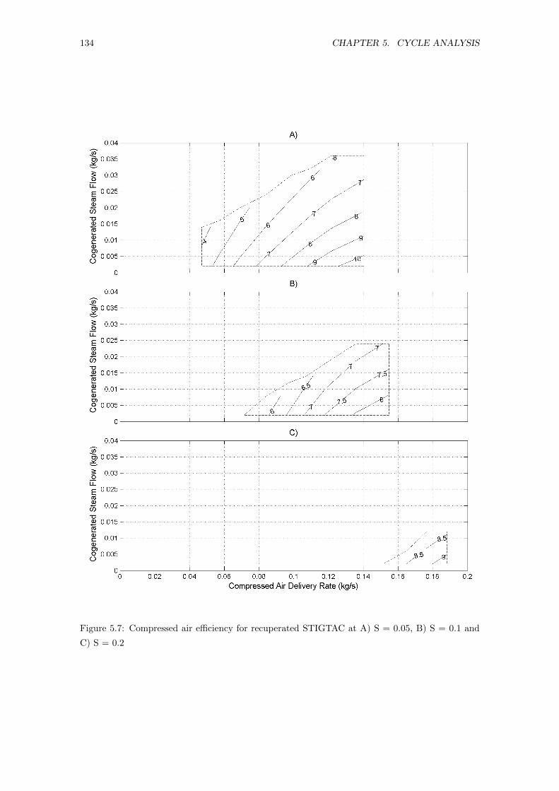
134 CHAPTER 5. CYCLE ANALYSIS
Figure 5.7: Compressed air efficiency for recuperated STIGTAC at A) S = 0.05, B) S = 0.1 and
C) S = 0.2
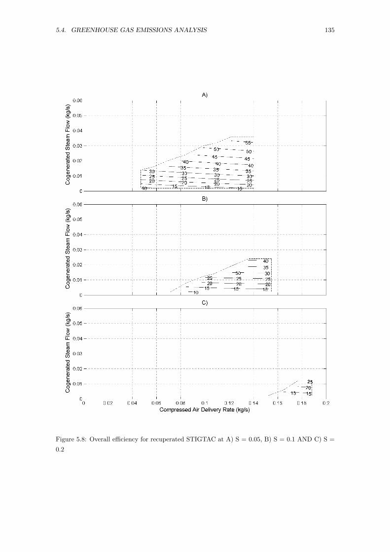
5.4. GREENHOUSE GAS EMISSIONS ANALYSIS 135
Figure 5.8: Overall efficiency for recuperated STIGTAC at A) S = 0.05, B) S = 0.1 AND C) S =
0.2
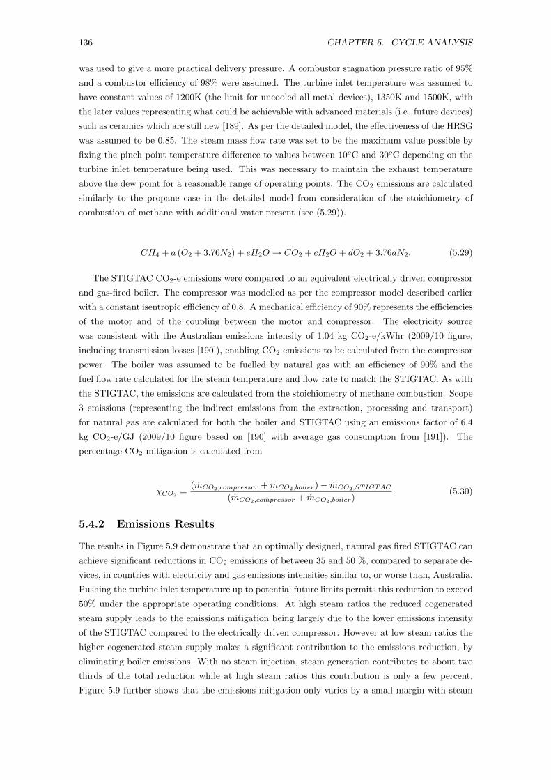
136 CHAPTER 5. CYCLE ANALYSIS
was used to give a more practical delivery pressure. A combustor stagnation pressure ratio of 95%
and a combustor efficiency of 98% were assumed. The turbine inlet temperature was assumed to
have constant values of 1200K (the limit for uncooled all metal devices), 1350K and 1500K, with
the later values representing what could be achievable with advanced materials (i.e. future devices)
such as ceramics which are still new [189]. As per the detailed model, the effectiveness of the HRSG
was assumed to be 0.85. The steam mass flow rate was set to be the maximum value possible by
fixing the pinch point temperature difference to values between 10oC and 30oC depending on the
turbine inlet temperature being used. This was necessary to maintain the exhaust temperature
above the dew point for a reasonable range of operating points. The CO2 emissions are calculated
similarly to the propane case in the detailed model from consideration of the stoichiometry of
combustion of methane with additional water present (see (5.29)).
CH4 + a (O2 + 3.76N2) + eH2O → CO2 + cH2O + dO2 + 3.76aN2. (5.29)
The STIGTAC CO2-e emissions were compared to an equivalent electrically driven compressor
and gas-fired boiler. The compressor was modelled as per the compressor model described earlier
with a constant isentropic efficiency of 0.8. A mechanical efficiency of 90% represents the efficiencies
of the motor and of the coupling between the motor and compressor. The electricity source
was consistent with the Australian emissions intensity of 1.04 kg CO2-e/kWhr (2009/10 figure,
including transmission losses [190]), enabling CO2 emissions to be calculated from the compressor
power. The boiler was assumed to be fuelled by natural gas with an efficiency of 90% and the
fuel flow rate calculated for the steam temperature and flow rate to match the STIGTAC. As with
the STIGTAC, the emissions are calculated from the stoichiometry of methane combustion. Scope
3 emissions (representing the indirect emissions from the extraction, processing and transport)
for natural gas are calculated for both the boiler and STIGTAC using an emissions factor of 6.4
kg CO2-e/GJ (2009/10 figure based on [190] with average gas consumption from [191]). The
percentage CO2 mitigation is calculated from
χCO2=
(mCO2,compressor + mCO2,boiler)− mCO2,STIGTAC
(mCO2,compressor + mCO2,boiler). (5.30)
5.4.2 Emissions Results
The results in Figure 5.9 demonstrate that an optimally designed, natural gas fired STIGTAC can
achieve significant reductions in CO2 emissions of between 35 and 50 %, compared to separate de-
vices, in countries with electricity and gas emissions intensities similar to, or worse than, Australia.
Pushing the turbine inlet temperature up to potential future limits permits this reduction to exceed
50% under the appropriate operating conditions. At high steam ratios the reduced cogenerated
steam supply leads to the emissions mitigation being largely due to the lower emissions intensity
of the STIGTAC compared to the electrically driven compressor. However at low steam ratios the
higher cogenerated steam supply makes a significant contribution to the emissions reduction, by
eliminating boiler emissions. With no steam injection, steam generation contributes to about two
thirds of the total reduction while at high steam ratios this contribution is only a few percent.
Figure 5.9 further shows that the emissions mitigation only varies by a small margin with steam
5.5. CONCLUSION 137
Figure 5.9: CO2 mitigation of natural gas fired STIGTAC at Tti = 1200K (�), 1350K (o), 1500K
(+)
ratio. Hence, comparable emissions reductions can be achieved by either simple cogeneration or
steam injection.
5.5 Conclusion
A set of cogeneration cycles including the straight cogeneration of steam and compressed air, steam
injection, and the incorporation of recuperation with steam injection have been examined. This
included a comparison with simple recuperation as a standard approach employed for improving
gas turbine efficiency at low pressure ratios. This examination required suitable measures for the
efficiencies of compressed air and steam production to be defined. These were defined based on the
ratio of ‘useful work’, or heat in the case of steam generation, required to produce the compressed
air or steam to the total heat addition from combustion.
The analysis of these cycles demonstrated the benefits of cogeneration, with the cogenerat-
ing GTAC type cycle achieving increased energy utilisation as would be expected. Incorporating
steam injection demonstrated improvements in both the efficiency and volume of compressed air
production. While a recuperated GTAC demonstrated the highest device efficiency, the absence of
cogeneration resulted in much lower energy utilisation. Unfortunately combining steam injection
and recuperation impaired both options with either insufficient exhaust temperature for recuper-
ation or significantly reduced steam production. Furthermore, for pressure ratios of seven to nine,
which is typical in an industrial air compressor, a recuperated cycle is is of limited thermodynamic
benefit.

138 CHAPTER 5. CYCLE ANALYSIS
Further analysis on the emissions for a practical, commercial scale, optimised device demon-
strated that simple cogeneration and steam injection are both capable of achieving significant
reductions in greenhouse gas emissions compared to fossil fuel based, conventional compressed air
and steam production. Furthermore, the simple addition of cogeneration is capable of achieving
comparable emission reductions even without steam injection. Steam injection does however offer
improved versatility with an additional control variable for balancing compressed air and steam
demands.
Chapter 6
Model Reduction of a
Cogeneraton System
6.1 Introduction
In the previous chapter the merits of cogeneration systems producing compressed air and steam
were examined, demonstrating that the use of cogeneration can lead to significant improvements in
efficiency and emissions reductions compared to the use of separate systems. Furthermore, the use
of advanced model-based control systems has the potential to offer significant improvements in plant
operation [36] with the implementation of model predictive control (MPC) on a combined cycle
power plant. The implementation of such control methods requires a suitable model, specifically
one that can be evaluated significantly faster than real time. While this can be less of an issue
for the slower dynamics of a large scale power plant, small scale devices, with typically faster
dynamics, require a correspondingly faster model. Hence, this chapter considers the development
of a reduced order cogeneration model suitable for control applications.
A high order cogeneration model is first defined using the cogeneration setup from the previous
chapter. While more advanced cycle configurations would be more versatile, only the general steam
and compressed air production case is considered. In contrast to the informal approach in Chapter
4, time scale separation and application of singular perturbation theory is used in this chapter for
model reduction. Three choices for time scale separation, and subsequent reduced order models,
are considered with their dynamic performance compared to the higher order model.
6.2 Cogeneration System and Model
The cogeneration system being considered in this chapter is constructed from the gas turbine air
compressor (GTAC) system presented by Wiese et al [9] and a basic drum boiler as presented
in Chapter 3. This system is shown schematically in Figure 6.1. The gas turbine section of the
system is modelled by the GTAC model developed by Wiese et al [3]. While the details of the gas
turbine model can be found in [3], with more detail also available in [1] the basic form of this model
is presented here for reference. Figure 6.2 shows the structure of the GTAC model including the
flow of the model states and inputs (excluding fuel conditions). The general form of the governing
139
140 CHAPTER 6. MODEL REDUCTION OF A COGENERATON SYSTEM
differential equations of the GTAC model are given by
Edz
dt= g (z,Twall, ω,u,md) , (6.1)
Jdω
dt= f1 (z,Twall, ω,md) , (6.2)
CwalldTwall
dt= f2 (z,Twall,md) , (6.3)
where
z = [M1, pt,2, s2,M2, pt,3, s3,M4, pt,5, s5, ...,M9, pt,10, s10]T, (6.4)
E = [εintake, εcomp, εcomb,duct, εcomb,exp, εburner, εconvergence, εturb, εexh] , (6.5)
Twall = [Twall,conv, Twall,turb, Twall,exh]T, (6.6)
Cwall =[ρwallVwallCp.wall|conv, ρwallVwallCp.wall|turb, ρwallVwallCp.wall|exh
], (6.7)
u = [cv,f , θbl] , (6.8)
md = [pt,1, Tt,1, ps,11, Tf , pf ] , (6.9)
with˜denoting non-dimensionalised variables and the model function inputs given by z the vector
of fluid component states, Twall a vector of relevent wall temperatures, ω the GTAC spool speed, u
a vector of the GTAC actuator positions, and md a set of measured disturbances. The remaining
terms, E and Cwall, contain model parameters with the later being the heat capacities of the
GTAC wall elements.
The models for the components of the drum boiler section of the cogeneration system are
modeled as described in Chapter 3 noting that with the exception of the feedpump this modelling
approach was validated in Chapter 4 against the Newport power plant. The feedpump model
was not validated as part of this process due to insufficient data. However, the feedpump model
presented in Chapter 3 is based on a well established approach by Leva and Maffezzoni [166] and as
such will be used here. Similarly to the Newport case in Chapter 4 it is assumed that the phase at
the inlet of the riser is subcooled meaning that the liquid to two-phase transition element is being
used. Since each of the boiler heat transfer components are being modelled as single elements this
means the two-phase model is not required.
Since this cogeneration system does not physically exist it is necessary to choose a scale such
that a suitable representative model can be defined. Since the GTAC model was validated by Wiese
et al [3] experimentally this scale is chosen for the model presented here. This allows the gas turbine
geometry and model parameters to be used unchanged as given in [3] while those corresponding to
the boiler can be set in accordance with this scale, which approximately corresponds to a 200kW
boiler. The geometry and properties of the boiler have been set based on several conditions.
Firstly it is desirable for these model terms to be consistent with existing commercial boilers
of this scale. However, the available information on commercial systems is fairly limited requiring
additional conditions to be considered. Secondly, while this representative system is of smaller
scale, the dynamic behaviour of the Newport boiler considered in Chapter 4 can be used as guide
for that of the smaller device. Hence, the geometry of the boiler can be set to be both consistent
with commercial devices and with the dynamic behaviour of the Newport boiler. Finally the heat
transfer conditions, namely the heat transfer coefficients, can be set based on remaining consistent
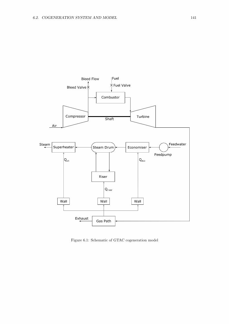
6.2. COGENERATION SYSTEM AND MODEL 141
Figure 6.1: Schematic of GTAC cogeneration model
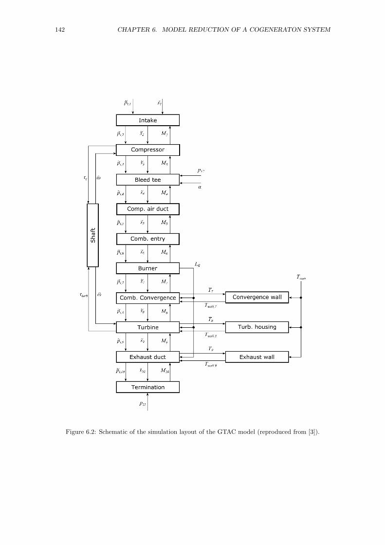
142 CHAPTER 6. MODEL REDUCTION OF A COGENERATON SYSTEM
Figure 6.2: Schematic of the simulation layout of the GTAC model (reproduced from [3]).
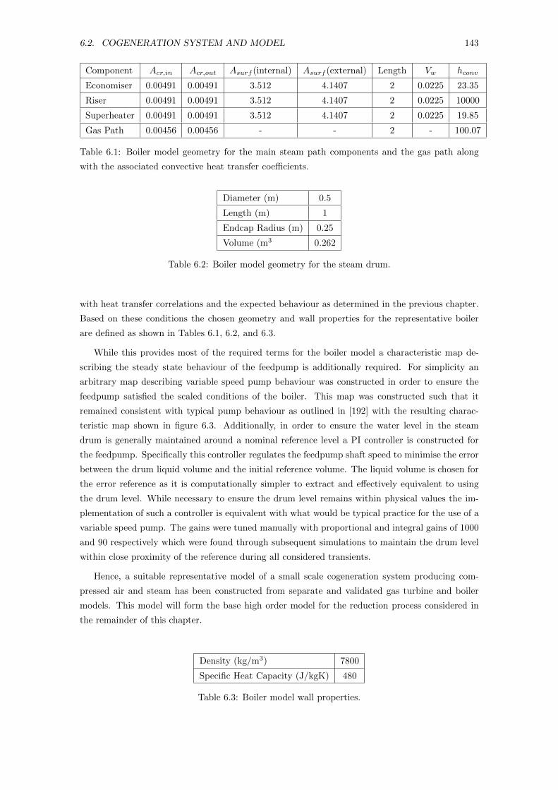
6.2. COGENERATION SYSTEM AND MODEL 143
Component Acr,in Acr,out Asurf (internal) Asurf (external) Length Vw hconv
Economiser 0.00491 0.00491 3.512 4.1407 2 0.0225 23.35
Riser 0.00491 0.00491 3.512 4.1407 2 0.0225 10000
Superheater 0.00491 0.00491 3.512 4.1407 2 0.0225 19.85
Gas Path 0.00456 0.00456 - - 2 - 100.07
Table 6.1: Boiler model geometry for the main steam path components and the gas path along
with the associated convective heat transfer coefficients.
Diameter (m) 0.5
Length (m) 1
Endcap Radius (m) 0.25
Volume (m3 0.262
Table 6.2: Boiler model geometry for the steam drum.
with heat transfer correlations and the expected behaviour as determined in the previous chapter.
Based on these conditions the chosen geometry and wall properties for the representative boiler
are defined as shown in Tables 6.1, 6.2, and 6.3.
While this provides most of the required terms for the boiler model a characteristic map de-
scribing the steady state behaviour of the feedpump is additionally required. For simplicity an
arbitrary map describing variable speed pump behaviour was constructed in order to ensure the
feedpump satisfied the scaled conditions of the boiler. This map was constructed such that it
remained consistent with typical pump behaviour as outlined in [192] with the resulting charac-
teristic map shown in figure 6.3. Additionally, in order to ensure the water level in the steam
drum is generally maintained around a nominal reference level a PI controller is constructed for
the feedpump. Specifically this controller regulates the feedpump shaft speed to minimise the error
between the drum liquid volume and the initial reference volume. The liquid volume is chosen for
the error reference as it is computationally simpler to extract and effectively equivalent to using
the drum level. While necessary to ensure the drum level remains within physical values the im-
plementation of such a controller is equivalent with what would be typical practice for the use of a
variable speed pump. The gains were tuned manually with proportional and integral gains of 1000
and 90 respectively which were found through subsequent simulations to maintain the drum level
within close proximity of the reference during all considered transients.
Hence, a suitable representative model of a small scale cogeneration system producing com-
pressed air and steam has been constructed from separate and validated gas turbine and boiler
models. This model will form the base high order model for the reduction process considered in
the remainder of this chapter.
Density (kg/m3) 7800
Specific Heat Capacity (J/kgK) 480
Table 6.3: Boiler model wall properties.
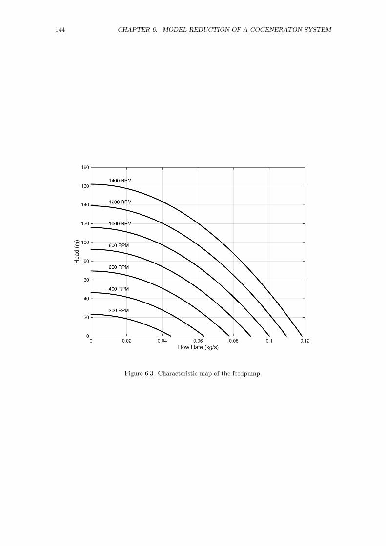
144 CHAPTER 6. MODEL REDUCTION OF A COGENERATON SYSTEM
Figure 6.3: Characteristic map of the feedpump.
6.3. MODEL REDUCTION 145
6.3 Model Reduction
While an informal model reduction process was considered previously for the Newport boiler in
Chapter 4 it is desirable here to define a formal process for reducing the model that can potentially
be applied to other comparable cogeneration systems. A model reduction process based on time
scale separation and singular perturbation theory has previously been considered by Wiese et al
[117] for the case of the GTAC. The reduction process considered here will extend this process for
the case of the cogeneration model described in the previous section.
In order for singular perturbation theory to be applicable the model has to first be expressed
in the form of a single perturbation model. This requires the conversion of the governing dynamic
equations to the non-dimensional form given by
dx
dt= f (z′,x,u,md) , (6.10)
ζdz′
dt= h′ (z′,x,u,md) , (6.11)
where ζ is the perturbation parameter while z′ and x represent two sets of state variables de-
scribed by the sets of differential equations given by h′ and f respectively. In the application of
singular perturbation theory the equations represented by (6.11) represent those whose dynamics
can be considered sufficiently fast enough to be treated as quasi-steady. Similarly, the equations
represented by (6.10) are those that are considered significant in terms of the dynamic response of
the system. The determination of these requires an examination of the time scales of the system
to determine an appropriate point at which they can be separated into these fast and slow dy-
namics. An analysis of these time scales is additionally required for determining the perturbation
parameter.
To determine these time scales it is necessary to determine suitable non-dimensional physical
inertia terms associated with the governing differential equations. Fortunately the GTAC model
developed by Wiese et al [3] is already set up in a non-dimensional form suitable for use with
singular perturbation theory and as such the required inertia terms for the gas turbine components
shown in Figure 6.2 are already available. These are the elements of E in the GTAC model shown
in (6.5) for the fluid components, while non-dimensional forms of J and Cwall for (6.2) and (6.3)
respectively round out the inertia terms for the gas turbine model. While more detail on these
terms can be found in [117] and [1] the equations describing these terms are presented here for
reference. The non-dimensional inertia term for the fluid model, ε, is given by
ε =L
t√γRTt
, (6.12)
where t is the reference time used in the non-dimensionalisation process and is kept general at
this stage. Recognising that the denominator is this reference time multiplied by the speed of
sound it can be seen that physically ε corresponds to the ratio of the residence time of a pressure
perturbation passing through the component to the chosen reference time.
The non dimensional shaft inertia is given by
J =J
tmcr2tipσslip
, (6.13)
146 CHAPTER 6. MODEL REDUCTION OF A COGENERATON SYSTEM
where mc is the mass flow rate through the compressor, rtip is the radius of the exducer tip, and
σslip is the slip factor which is the ratio of the tangenetial gas velocity leaving the impeller vanes
to the impeller tip speed.
Similarly the non-dimensional heat capacity is given by
Cwall =ρwallVwallCwall
thintAint, (6.14)
where hint and Aint correspond to the heat transfer coefficient and surface area for internal side of
the component wall. Additionally it can be noted that (6.14) is consistent with the standard form
of the time constant for transient convective heat transfer from a solid body [193].
While this provides a suitable set of non-dimensional inertia terms for the gas turbine section
the boiler model developed in Chapter 3 is not in non-dimensional form. Hence, it is necessary to
convert this model to non-dimensional form and determine suitable inertia terms for the governing
differential equations of the boiler. Fortunately, since the two-phase fluid model is not required only
the single-phase model and wall model of the boiler will need to be considered. Similarly, as per
the consideration of the Newport boiler, full reduction of the steam drum is not considered as these
states need to be retained to ensure the drum level can be modelled. Hence, non-dimensionalisation
of the drum model is not considered.
6.3.1 Single-Phase Model Non-Dimensionalisation
The determination of suitable non-dimensional inertia terms for the single-phase components re-
quires the conversion of the single-phase model presented in Chapter 3 to a non-dimensional form.
The general non-discretised form of the single-phase model (expressed in matrix form by (3.8) to
(3.11)) can alternatively be expressed as a set of equations given by
∂ρ
∂t= −u∂ρ
∂y− ρ∂u
∂y+ f1, (6.15)
∂Ps∂t
= −u∂Ps∂y−Ps − ρ2 ∂e
∂ρ
ρ ∂e∂Ps
∂u
∂y+ f2, (6.16)
∂u
∂t= −1
ρ
∂Ps∂y− u∂u
∂y+ f3, (6.17)
where fi refers to the forcing terms. In non-dimensionalising this set of equations it is necessary
to first define a set of suitable non-dimensional terms for substitution. Following the same general
principles as used by Badmus et al [14, 15] and Wiese et al [3] a set of non-dimensional terms can
be defined as given in Table 6.4. Using these expressions the relevant terms of (6.15) to (6.17) can
be expressed in non-dimensional terms.
The details of this non-dimensionalistion process can be found in Appendix C. The non-
dimensional form of (6.15) is given by
L
c
∂ρ
∂t= M
∂ρ
∂y− ∂M
∂y− M
c
(∂c
∂ρ
∂ρ
∂y+
∂c
∂Ps
∂Ps∂y
)+ f1. (6.18)
The non-dimensional form of (6.16) is given by
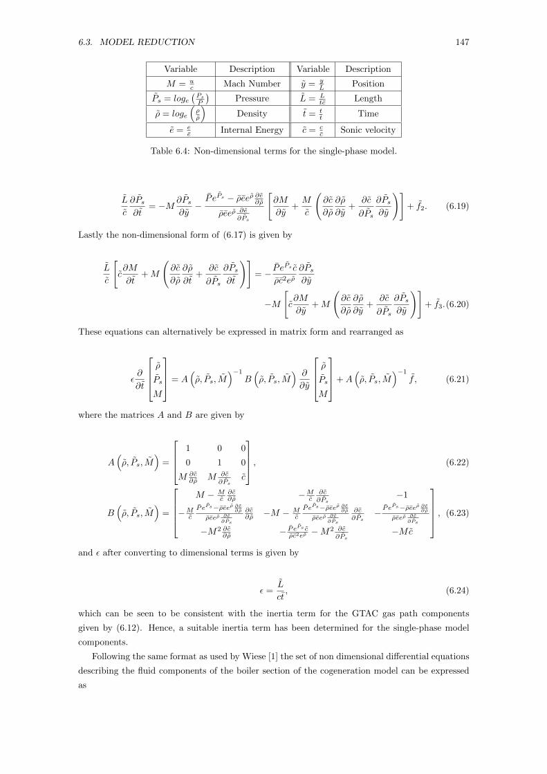
6.3. MODEL REDUCTION 147
Variable Description Variable Description
M = uc Mach Number y = y
L Position
Ps = loge(PsP
)Pressure L = L
tc Length
ρ = loge
(ρρ
)Density t = t
t Time
e = ee Internal Energy c = c
c Sonic velocity
Table 6.4: Non-dimensional terms for the single-phase model.
L
c
∂Ps
∂t= −M ∂Ps
∂y−P ePs − ρeeρ ∂e∂ρ
ρeeρ ∂e∂Ps
[∂M
∂y+M
c
(∂c
∂ρ
∂ρ
∂y+
∂c
∂Ps
∂Ps∂y
)]+ f2. (6.19)
Lastly the non-dimensional form of (6.17) is given by
L
c
[c∂M
∂t+M
(∂c
∂ρ
∂ρ
∂t+
∂c
∂Ps
∂Ps
∂t
)]= − P e
Ps c
ρc2eρ∂Ps∂y
−M
[c∂M
∂y+M
(∂c
∂ρ
∂ρ
∂y+
∂c
∂Ps
∂Ps∂y
)]+ f3.(6.20)
These equations can alternatively be expressed in matrix form and rearranged as
ε∂
∂t
ρ
Ps
M
= A(ρ, Ps, M
)−1
B(ρ, Ps, M
) ∂
∂y
ρ
Ps
M
+A(ρ, Ps, M
)−1
f , (6.21)
where the matrices A and B are given by
A(ρ, Ps, M
)=
1 0 0
0 1 0
M ∂c∂ρ M ∂c
∂Psc
, (6.22)
B(ρ, Ps, M
)=
M − M
c∂c∂ρ −Mc
∂c∂Ps
−1
−McPePs−ρeeρ ∂e∂ρρeeρ ∂e
∂Ps
∂c∂ρ −M − M
c
PePs−ρeeρ ∂e∂ρρeeρ ∂e
∂Ps
∂c∂Ps
− P ePs−ρeeρ ∂e∂ρρeeρ ∂e
∂Ps
−M2 ∂c∂ρ − P e
Ps cρc2eρ −M
2 ∂c∂Ps
−Mc
, (6.23)
and ε after converting to dimensional terms is given by
ε =L
ct, (6.24)
which can be seen to be consistent with the inertia term for the GTAC gas path components
given by (6.12). Hence, a suitable inertia term has been determined for the single-phase model
components.
Following the same format as used by Wiese [1] the set of non dimensional differential equations
describing the fluid components of the boiler section of the cogeneration model can be expressed
as
148 CHAPTER 6. MODEL REDUCTION OF A COGENERATON SYSTEM
Eb∂zb
∂t= gb (zb,Tb,wall,u,md) , (6.25)
where the set of boiler fluid component inertia terms, Eb is given by
Eb = [εeco, εriser, εsh, εgas] , (6.26)
zb is the vector of states for the boiler fluid components as described in Chapter 3, and Tb,wall
is the vector of boiler wall temperatures. The inputs u remain unchanged from (6.8) and the
measured disturbances md include the addition of the feedwater inlet pressure and temperature.
6.3.2 Wall Model
The wall model used in the boiler model is comparable to that used by Wiese et al [3, 117] and as
such the non-dimensionalistion results in the same basic form of the inertia term. Hence, (6.14)
can be used for calculating the inertia terms for the boiler walls. For these components the gas
path heat transfer coefficient and surface area are chosen for use in this calculation as previous
work in Chapter 4 demonstrated that the gas path heat transfer was more dynamically dominant
than that from the steam path.
By the same process as the single-phase model, the set of non-dimensional differential equations
describing the boiler wall temperatures can be expressed as
Cb,wall∂Tb.wall
∂t=
1
Qbfb (zb,Tb,wall,md) , (6.27)
where Cwall is the vector of non-dimensional wall capacities for the boiler wall components given
by
Cb,wall = [Cwall,eco, Cwall,riser, Cwall,sh]. (6.28)
Qb is the reference heat transfer for the boiler defined as per [117] and fb is the vector of differential
equations for the economiser, riser, and superheater wall temperatures as given in Chapter 3
converted to non-dimensional form. The remaining inputs zb, Tb,wall, and md are as defined
previously.
6.3.3 Cogeneration System Model Reduction
6.3.3.1 Time Scale Comparison
With suitable expressions determined for the boiler component’s non-dimensional inertia terms
and corresponding GTAC terms already available from [117] the separation of time scales of the
cogeneration model can be examined. Since the choice of reference time, t, has not been made yet
and this quantity is in the denominator of each inertia term the resulting values will be considered
as multiples of t. The resulting maximum and minimum inertia terms, calculated for the nom-
inal operating range of the cogeneration system, for both the boiler components and the GTAC
components are shown in Table 6.5.
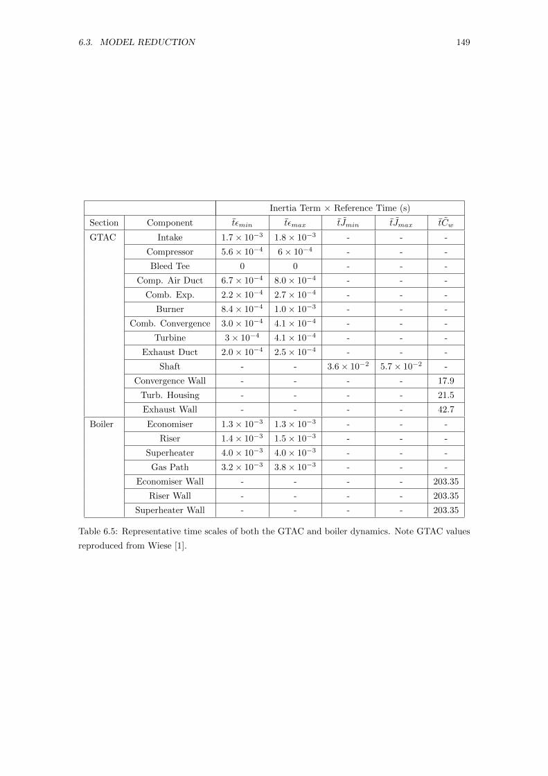
6.3. MODEL REDUCTION 149
Inertia Term × Reference Time (s)
Section Component tεmin tεmax tJmin tJmax tCw
GTAC Intake 1.7× 10⁻³ 1.8× 10⁻³ - - -
Compressor 5.6× 10⁻⁴ 6× 10⁻⁴ - - -
Bleed Tee 0 0 - - -
Comp. Air Duct 6.7× 10⁻⁴ 8.0× 10⁻⁴ - - -
Comb. Exp. 2.2× 10⁻⁴ 2.7× 10⁻⁴ - - -
Burner 8.4× 10⁻⁴ 1.0× 10⁻³ - - -
Comb. Convergence 3.0× 10⁻⁴ 4.1× 10⁻⁴ - - -
Turbine 3× 10⁻⁴ 4.1× 10⁻⁴ - - -
Exhaust Duct 2.0× 10⁻⁴ 2.5× 10⁻⁴ - - -
Shaft - - 3.6× 10⁻² 5.7× 10⁻² -
Convergence Wall - - - - 17.9
Turb. Housing - - - - 21.5
Exhaust Wall - - - - 42.7
Boiler Economiser 1.3× 10⁻³ 1.3× 10⁻³ - - -
Riser 1.4× 10⁻³ 1.5× 10⁻³ - - -
Superheater 4.0× 10⁻³ 4.0× 10⁻³ - - -
Gas Path 3.2× 10⁻³ 3.8× 10⁻³ - - -
Economiser Wall - - - - 203.35
Riser Wall - - - - 203.35
Superheater Wall - - - - 203.35
Table 6.5: Representative time scales of both the GTAC and boiler dynamics. Note GTAC values
reproduced from Wiese [1].
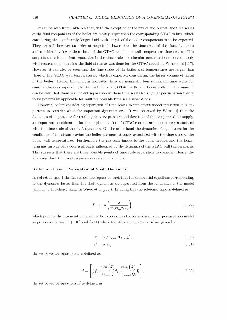
150 CHAPTER 6. MODEL REDUCTION OF A COGENERATON SYSTEM
It can be seen from Table 6.5 that, with the exception of the intake and burner, the time scales
of the fluid components of the boiler are mostly larger than the corresponding GTAC values, which
considering the significantly longer fluid path length of the boiler components is to be expected.
They are still however an order of magnitude lower than the time scale of the shaft dynamics
and considerably lower than those of the GTAC and boiler wall temperature time scales. This
suggests there is sufficient separation in the time scales for singular perturbation theory to apply
with regards to eliminating the fluid states as was done for the GTAC model by Wiese et al [117].
However, it can also be seen that the time scales of the boiler wall temperatures are larger than
those of the GTAC wall temperatures, which is expected considering the larger volume of metal
in the boiler. Hence, this analysis indicates there are nominally four significant time scales for
consideration corresponding to the the fluid, shaft, GTAC walls, and boiler walls. Furthermore, it
can be seen that there is sufficient separation in these time scales for singular perturbation theory
to be potentially applicable for multiple possible time scale separations.
However, before considering separation of time scales to implement model reduction it is im-
portant to consider what the important dynamics are. It was observed by Wiese [1] that the
dynamics of importance for tracking delivery pressure and flow rate of the compressed air supply,
an important consideration for the implementation of GTAC control, are most closely associated
with the time scale of the shaft dynamics. On the other hand the dynamics of significance for the
conditions of the steam leaving the boiler are more strongly associated with the time scale of the
boiler wall temperatures. Furthermore the gas path inputs to the boiler section and the longer
term gas turbine behaviour is strongly influenced by the dynamics of the GTAC wall temperatures.
This suggests that there are three possible points of time scale separation to consider. Hence, the
following three time scale separation cases are examined.
Reduction Case 1: Separation at Shaft Dynamics
In reduction case 1 the time scales are separated such that the differential equations corresponding
to the dynamics faster than the shaft dynamics are separated from the remainder of the model
(similar to the choice made in Wiese et al [117]). In doing this the reference time is defined as
t = min
(J
mcr2tipσslip
), (6.29)
which permits the cogeneration model to be expressed in the form of a singular perturbation model
as previously shown in (6.10) and (6.11) where the state vectors x and z′ are given by
x = [ω,Twall,Tb,wall] , (6.30)
z′ = [z, zb] , (6.31)
the set of vector equations f is defined as
f =
1
τf1,
min(J)
CwallQf2,
min(J)
Cb,wallQbfb
, (6.32)
the set of vector equations h′ is defined as
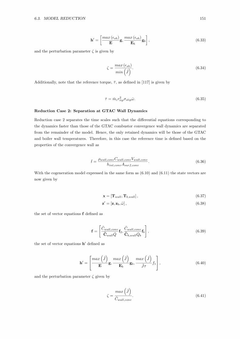
6.3. MODEL REDUCTION 151
h′ =
[max (εsh)
Eg,max (εsh)
Ebgb
], (6.33)
and the perturbation parameter ζ is given by
ζ =max (εsh)
min(J) . (6.34)
Additionally, note that the reference torque, τ , as defined in [117] is given by
τ = mcr2tipσslipω. (6.35)
Reduction Case 2: Separation at GTAC Wall Dynamics
Reduction case 2 separates the time scales such that the differential equations corresponding to
the dynamics faster than those of the GTAC combustor convergence wall dynamics are separated
from the remainder of the model. Hence, the only retained dynamics will be those of the GTAC
and boiler wall temperatures. Therefore, in this case the reference time is defined based on the
properties of the convergence wall as
t =ρwall,convCwall,convVwall,conv
hint,convAsurf,conv. (6.36)
With the cogeneration model expressed in the same form as (6.10) and (6.11) the state vectors are
now given by
x = [Twall,Tb,wall] , (6.37)
z′ = [z, zb, ω] , (6.38)
the set of vector equations f defined as
f =
[Cwall,conv
CwallQf2,
Cwall,conv
Cb,wallQbfb
], (6.39)
the set of vector equations h′ defined as
h′ =
max(J)
Eg,max
(J)
Ebgb,
max(J)
J τf1
, (6.40)
and the perturbation parameter ζ given by
ζ =max
(J)
Cwall,conv. (6.41)
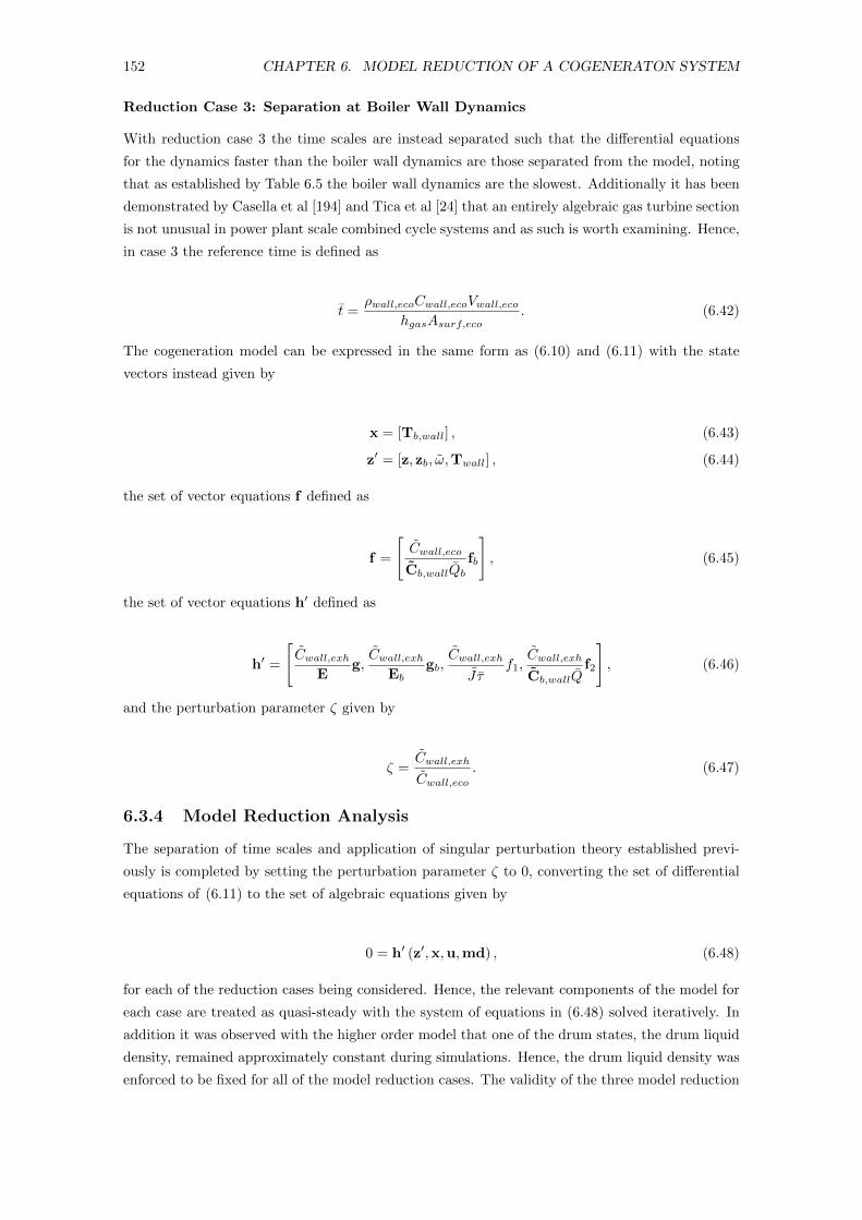
152 CHAPTER 6. MODEL REDUCTION OF A COGENERATON SYSTEM
Reduction Case 3: Separation at Boiler Wall Dynamics
With reduction case 3 the time scales are instead separated such that the differential equations
for the dynamics faster than the boiler wall dynamics are those separated from the model, noting
that as established by Table 6.5 the boiler wall dynamics are the slowest. Additionally it has been
demonstrated by Casella et al [194] and Tica et al [24] that an entirely algebraic gas turbine section
is not unusual in power plant scale combined cycle systems and as such is worth examining. Hence,
in case 3 the reference time is defined as
t =ρwall,ecoCwall,ecoVwall,eco
hgasAsurf,eco. (6.42)
The cogeneration model can be expressed in the same form as (6.10) and (6.11) with the state
vectors instead given by
x = [Tb,wall] , (6.43)
z′ = [z, zb, ω,Twall] , (6.44)
the set of vector equations f defined as
f =
[Cwall,eco
Cb,wallQbfb
], (6.45)
the set of vector equations h′ defined as
h′ =
[Cwall,exh
Eg,Cwall,exh
Ebgb,
Cwall,exh
J τf1,
Cwall,exh
Cb,wallQf2
], (6.46)
and the perturbation parameter ζ given by
ζ =Cwall,exh
Cwall,eco. (6.47)
6.3.4 Model Reduction Analysis
The separation of time scales and application of singular perturbation theory established previ-
ously is completed by setting the perturbation parameter ζ to 0, converting the set of differential
equations of (6.11) to the set of algebraic equations given by
0 = h′ (z′,x,u,md) , (6.48)
for each of the reduction cases being considered. Hence, the relevant components of the model for
each case are treated as quasi-steady with the system of equations in (6.48) solved iteratively. In
addition it was observed with the higher order model that one of the drum states, the drum liquid
density, remained approximately constant during simulations. Hence, the drum liquid density was
enforced to be fixed for all of the model reduction cases. The validity of the three model reduction
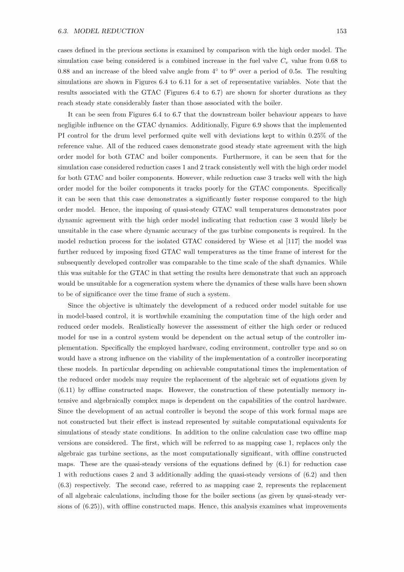
6.3. MODEL REDUCTION 153
cases defined in the previous sections is examined by comparison with the high order model. The
simulation case being considered is a combined increase in the fuel valve Cv value from 0.68 to
0.88 and an increase of the bleed valve angle from 4◦ to 9◦ over a period of 0.5s. The resulting
simulations are shown in Figures 6.4 to 6.11 for a set of representative variables. Note that the
results associated with the GTAC (Figures 6.4 to 6.7) are shown for shorter durations as they
reach steady state considerably faster than those associated with the boiler.
It can be seen from Figures 6.4 to 6.7 that the downstream boiler behaviour appears to have
negligible influence on the GTAC dynamics. Additionally, Figure 6.9 shows that the implemented
PI control for the drum level performed quite well with deviations kept to within 0.25% of the
reference value. All of the reduced cases demonstrate good steady state agreement with the high
order model for both GTAC and boiler components. Furthermore, it can be seen that for the
simulation case considered reduction cases 1 and 2 track consistently well with the high order model
for both GTAC and boiler components. However, while reduction case 3 tracks well with the high
order model for the boiler components it tracks poorly for the GTAC components. Specifically
it can be seen that this case demonstrates a significantly faster response compared to the high
order model. Hence, the imposing of quasi-steady GTAC wall temperatures demonstrates poor
dynamic agreement with the high order model indicating that reduction case 3 would likely be
unsuitable in the case where dynamic accuracy of the gas turbine components is required. In the
model reduction process for the isolated GTAC considered by Wiese et al [117] the model was
further reduced by imposing fixed GTAC wall temperatures as the time frame of interest for the
subsequently developed controller was comparable to the time scale of the shaft dynamics. While
this was suitable for the GTAC in that setting the results here demonstrate that such an approach
would be unsuitable for a cogeneration system where the dynamics of these walls have been shown
to be of significance over the time frame of such a system.
Since the objective is ultimately the development of a reduced order model suitable for use
in model-based control, it is worthwhile examining the computation time of the high order and
reduced order models. Realistically however the assessment of either the high order or reduced
model for use in a control system would be dependent on the actual setup of the controller im-
plementation. Specifically the employed hardware, coding environment, controller type and so on
would have a strong influence on the viability of the implementation of a controller incorporating
these models. In particular depending on achievable computational times the implementation of
the reduced order models may require the replacement of the algebraic set of equations given by
(6.11) by offline constructed maps. However, the construction of these potentially memory in-
tensive and algebraically complex maps is dependent on the capabilities of the control hardware.
Since the development of an actual controller is beyond the scope of this work formal maps are
not constructed but their effect is instead represented by suitable computational equivalents for
simulations of steady state conditions. In addition to the online calculation case two offline map
versions are considered. The first, which will be referred to as mapping case 1, replaces only the
algebraic gas turbine sections, as the most computationally significant, with offline constructed
maps. These are the quasi-steady versions of the equations defined by (6.1) for reduction case
1 with reductions cases 2 and 3 additionally adding the quasi-steady versions of (6.2) and then
(6.3) respectively. The second case, referred to as mapping case 2, represents the replacement
of all algebraic calculations, including those for the boiler sections (as given by quasi-steady ver-
sions of (6.25)), with offline constructed maps. Hence, this analysis examines what improvements
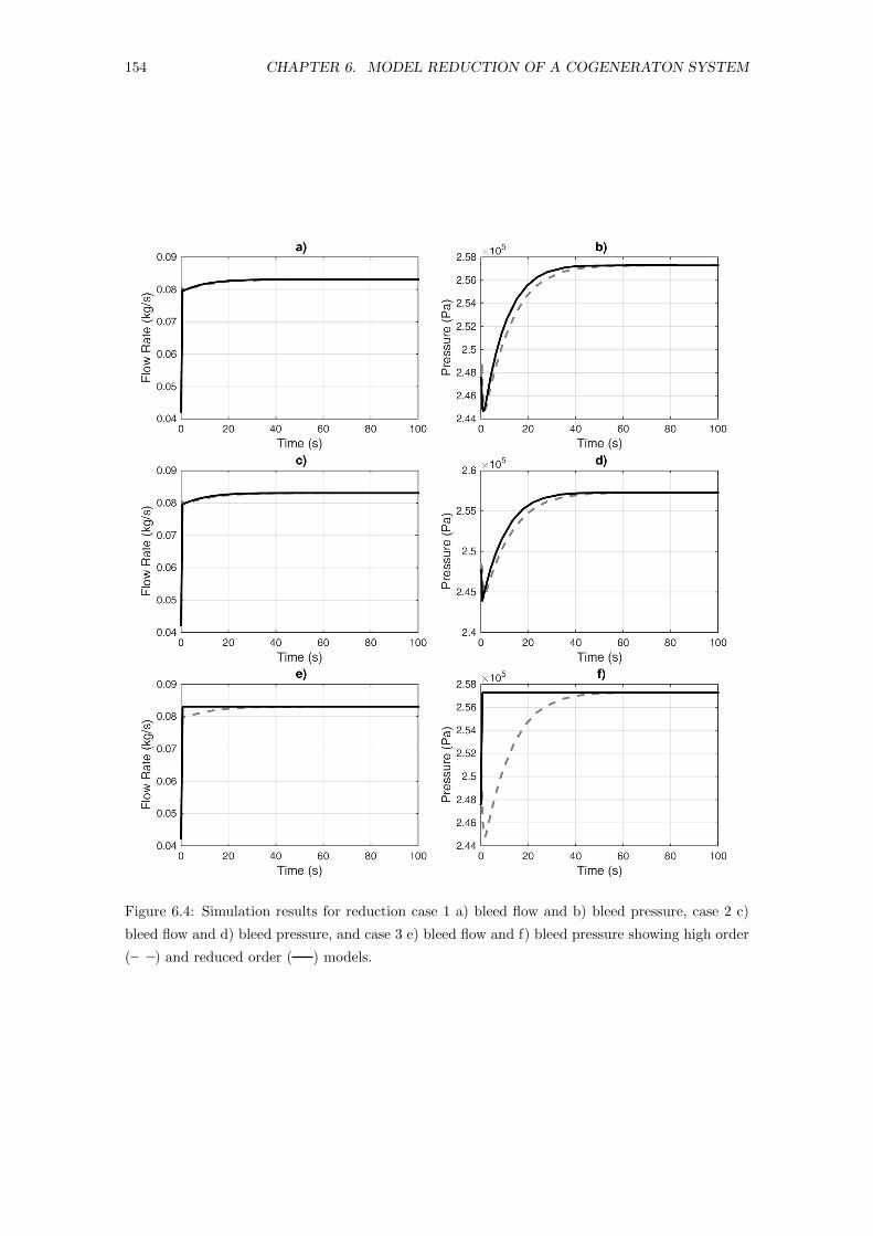
154 CHAPTER 6. MODEL REDUCTION OF A COGENERATON SYSTEM
Figure 6.4: Simulation results for reduction case 1 a) bleed flow and b) bleed pressure, case 2 c)
bleed flow and d) bleed pressure, and case 3 e) bleed flow and f) bleed pressure showing high order
( ) and reduced order ( ) models.
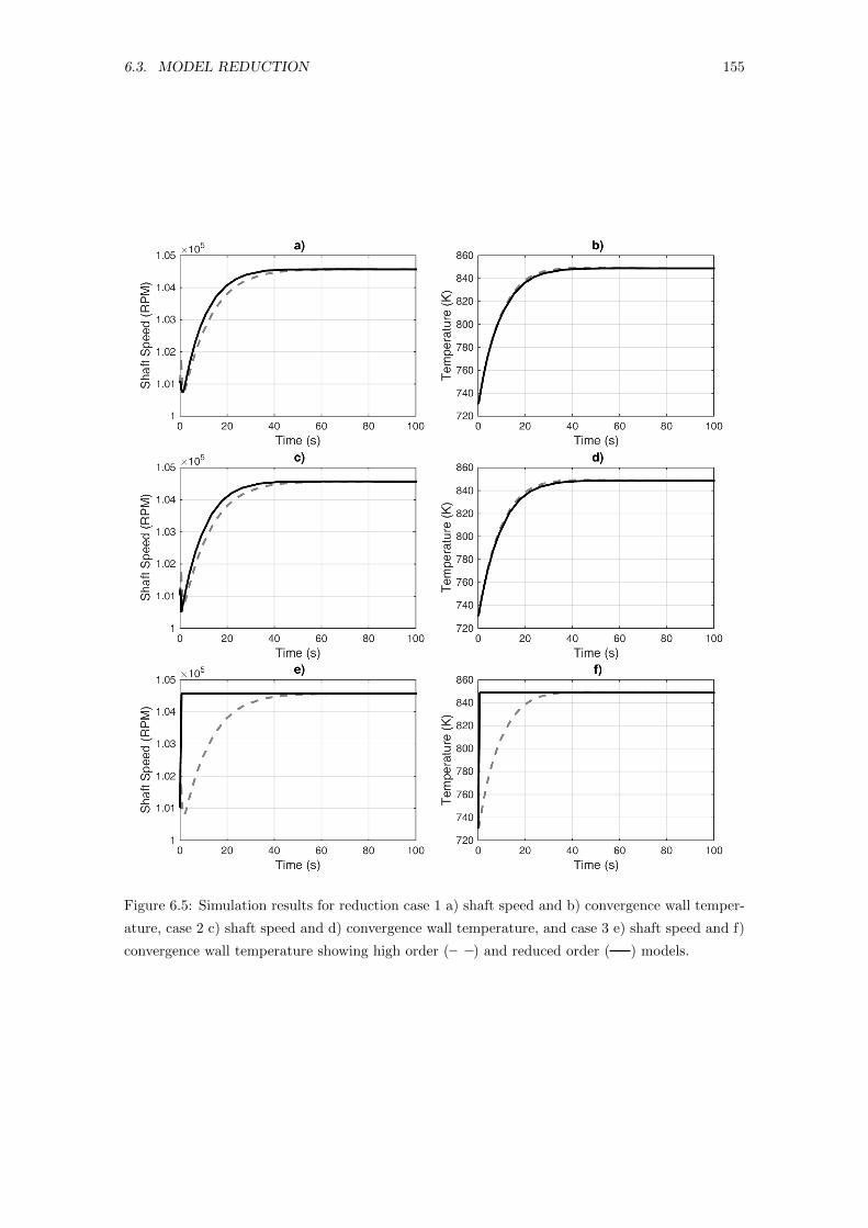
6.3. MODEL REDUCTION 155
Figure 6.5: Simulation results for reduction case 1 a) shaft speed and b) convergence wall temper-
ature, case 2 c) shaft speed and d) convergence wall temperature, and case 3 e) shaft speed and f)
convergence wall temperature showing high order ( ) and reduced order ( ) models.
156 CHAPTER 6. MODEL REDUCTION OF A COGENERATON SYSTEM
Figure 6.6: Simulation results for reduction case 1 a) turbine wall temperature and b) exhaust wall
temperature, case 2 c) turbine wall temperature and d) exhaust wall temperature, and case 3 e)
turbine wall temperature and f) exhaust wall temperature showing high order ( ) and reduced
order ( ) models.
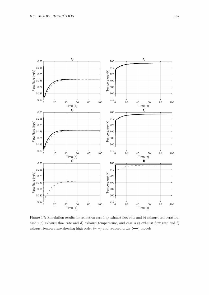
6.3. MODEL REDUCTION 157
Figure 6.7: Simulation results for reduction case 1 a) exhaust flow rate and b) exhaust temperature,
case 2 c) exhaust flow rate and d) exhaust temperature, and case 3 e) exhaust flow rate and f)
exhaust temperature showing high order ( ) and reduced order ( ) models.
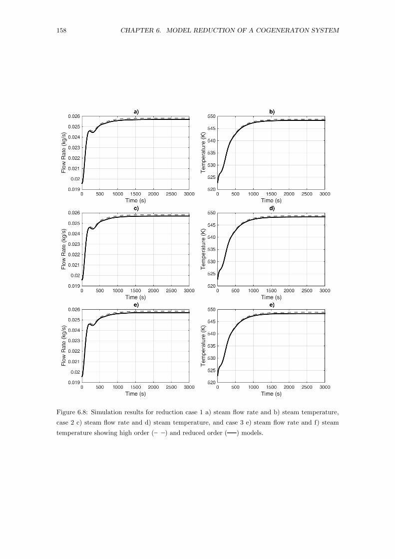
158 CHAPTER 6. MODEL REDUCTION OF A COGENERATON SYSTEM
Figure 6.8: Simulation results for reduction case 1 a) steam flow rate and b) steam temperature,
case 2 c) steam flow rate and d) steam temperature, and case 3 e) steam flow rate and f) steam
temperature showing high order ( ) and reduced order ( ) models.
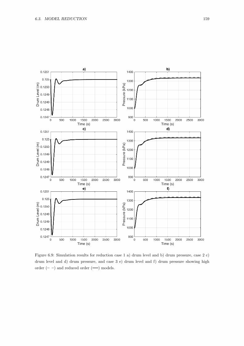
6.3. MODEL REDUCTION 159
Figure 6.9: Simulation results for reduction case 1 a) drum level and b) drum pressure, case 2 c)
drum level and d) drum pressure, and case 3 e) drum level and f) drum pressure showing high
order ( ) and reduced order ( ) models.
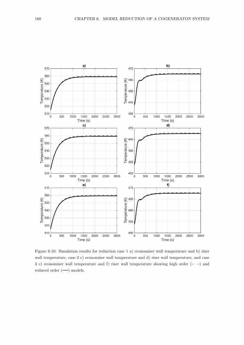
160 CHAPTER 6. MODEL REDUCTION OF A COGENERATON SYSTEM
Figure 6.10: Simulation results for reduction case 1 a) economiser wall temperature and b) riser
wall temperature, case 2 c) economiser wall temperature and d) riser wall temperature, and case
3 e) economiser wall temperature and f) riser wall temperature showing high order ( ) and
reduced order ( ) models.
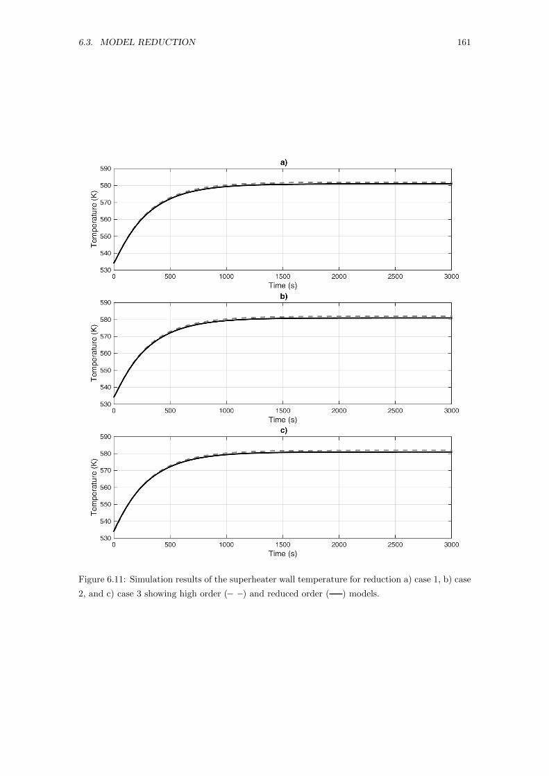
6.3. MODEL REDUCTION 161
Figure 6.11: Simulation results of the superheater wall temperature for reduction a) case 1, b) case
2, and c) case 3 showing high order ( ) and reduced order ( ) models.
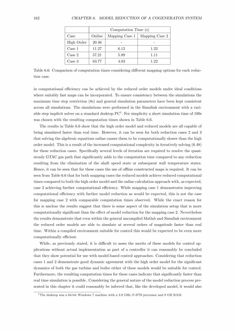
162 CHAPTER 6. MODEL REDUCTION OF A COGENERATON SYSTEM
Computation Time (s)
Case Online Mapping Case 1 Mapping Case 2
High Order 20.46 - -
Case 1 11.27 6.12 1.22
Case 2 57.21 5.89 1.11
Case 3 63.77 4.83 1.22
Table 6.6: Comparison of computation times considering different mapping options for each reduc-
tion case.
in computational efficiency can be achieved by the reduced order models under ideal conditions
where suitably fast maps can be incorporated. To ensure consistency between the simulations the
maximum time step restriction (8s) and general simulation parameters have been kept consistent
across all simulations. The simulations were performed in the Simulink environment with a vari-
able step implicit solver on a standard desktop PC1. For simplicity a short simulation time of 100s
was chosen with the resulting computation times shown in Table 6.6.
The results in Table 6.6 show that the high order model and reduced models are all capable of
being simulated faster than real time. However, it can be seen for both reduction cases 2 and 3
that solving the algebraic equations online causes them to be computationally slower than the high
order model. This is a result of the increased computational complexity in iteratively solving (6.48)
for these reduction cases. Specifically several levels of iteration are required to resolve the quasi-
steady GTAC gas path that significantly adds to the computation time compared to any reduction
resulting from the elimination of the shaft speed state or subsequent wall temperature states.
Hence, it can be seen that for these cases the use of offline constructed maps is required. It can be
seen from Table 6.6 that for both mapping cases the reduced models achieve reduced computational
times compared to both the high order model and the online calculation approach with, as expected,
case 2 achieving further computational efficiency. While mapping case 1 demonstrates improving
computational efficiency with further model reduction as would be expected, this is not the case
for mapping case 2 with comparable computation times observed. While the exact reason for
this is unclear the results suggest that there is some aspect of the simulation setup that is more
computationally significant than the effect of model reduction for the mapping case 2. Nevertheless
the results demonstrate that even within the general uncompiled Matlab and Simulink environment
the reduced order models are able to simulate at several orders of magnitude faster than real
time. Within a compiled environment suitable for control this would be expected to be even more
computationally efficient.
While, as previously stated, it is difficult to asses the merits of these models for control ap-
plications without actual implementation as part of a controller it can reasonably be concluded
that they show potential for use with model-based control approaches. Considering that reduction
cases 1 and 2 demonstrate good dynamic agreement with the high order model for the significant
dynamics of both the gas turbine and boiler either of these models would be suitable for control.
Furthermore, the resulting computation times for these cases indicate that significantly faster than
real time simulation is possible. Considering the general nature of the model reduction process pre-
sented in this chapter it could reasonably be inferred that, like the developed model, it would also
1The desktop was a 64-bit Windows 7 machine with a 3.9 GHz i7-3770 processor and 8 GB RAM.

6.4. CONCLUSION 163
be suitable for application to larger scale devices. Some consideration would however need to given
for differences that may result from the different time scales resulting from different sized devices
and the potential computational differences from differently constructed cogeneration systems.
6.4 Conclusion
This chapter first presented a dynamic model of a gas turbine based cogeneration system that pro-
duced compressed air and steam, before subsequently presenting a systematic method for reducing
this model’s order. The cogeneration model integrated the gas turbine air compressor (GTAC)
model of Wiese et al [3] with the boiler model presented in Chapter 3. The model reduction
method was implemented using time scale separation and singular perturbation theory. This first
required the conversion of the differential equations of the boiler model to a non-dimensional form
with representative inertia terms enabling comparison of the relevant component’s time scales.
This comparison, along with the results of [117], suggested that the gas turbine’s shaft time scale,
the gas turbine’s wall temperature time scale, and the boiler’s wall temperature time scale were
the three most significant time scales in this problem.
Three reduced order models with time scale separation defined at the shaft, gas turbine’s wall
temperatures, and boiler’s wall temperatures time scales respectively were then compared. This
showed that elimination of the gas turbine’s shaft dynamics did not significantly affect the cogener-
ation system model. However, whilst eliminating the gas turbines wall temperature dynamics did
not compromise the boiler dynamics, it still led to a reduction in the accuracy of the gas turbine
modelling. This suggested that at least two time scales, one for each of the gas turbine’s and the
boiler’s wall temperatures, needed to be retained in order to have a useful, reduced order dynamic
model of the cogeneration system.
Subsequent consideration of the computational efficiency of the models demonstrated that
further reduction beyond eliminating the dynamics of the fluid states requires the inclusion of
offline maps to accomodate the resulting increased algebraic complexity. This demonstrated that
significant improvements in computational efficiency are possible. The resulting computation times
demonstrate that significantly faster than real time simulation was possible, indicating that the
reduced order models are potentially suitable for use with model predictive control.

164 CHAPTER 6. MODEL REDUCTION OF A COGENERATON SYSTEM
Chapter 7
Conclusions and Future Work
This thesis presented a physics based model of a boiler and then demonstrated how this model
may be simplified using time scale separation and singular perturbation theory. The merits of the
cogeneration of compressed air and steam were also examined through cycle analysis.
The following contributions were made:
• The extension of a 1D nonlinear physics based, dynamic modelling framework to non-ideal,
single-phase and pure two-phase boiling fluids.
• The demonstration of the improvements in energy utilisation and emissions by the cogener-
ation of compressed air and steam along with potential further performance improvements
by incorporating steam injection.
• The development and demonstration of a model reduction process for a gas turbine based
cogeneration system.
While specific boiler and cogeneration applications were considered in this thesis, the model
and the model reduction process are more generally applicable.
7.1 Conclusions
The conclusions of this thesis are presented here in terms of the research aims given in Chapter 2.
1. To develop and validate a physics based 1D nonlinear model of a boiler
The literature review discussed how nonlinear model predictive control (NMPC) was a promising
method for controlling individual and cogeneration plants. This is primarily because NMPC in-
corporates constraint handling into the control law. Developing a high order model for subsequent
model reduction ensures a higher level of accuracy and provides a suitable plant model for sub-
sequent controller testing. Since a suitable gas turbine model has been developed by Wiese et al
[3] using the modelling framework of Badmus et al [13, 14, 15], a consistent boiler model is now
required.
The modelling framework developed by Badmus et al, while intended for ideal gas systems,
offered several important advantages over conventional modelling approaches. Firstly, this frame-
work was well suited for model reduction through singular perturbation and time scale separation.
Secondly, the original source terms are replaced by forcing term maps that can be defined in terms
165
166 CHAPTER 7. CONCLUSIONS AND FUTURE WORK
of steady state information, thus eliminating the need for dynamic studies. The developed boiler
model therefore extended this framework to include non-ideal, single-phase fluids and boiling,
two-phase fluids with the appropriate influence coefficients and forcing terms. The steady state
forcing term mapping functions were defined for adiabatic pipes, uniform cross-sectional area heat
transfer, and adiabatic cross sectional area change for both single and two-phase fluids. These
types of components described many of the main heat transfer and connecting components of a
conventional drum boiler. An additional general component for the transition from a single-phase
liquid to a two-phase fluid was also defined for the upstream end of the riser. Beyond these, ad-
ditional models were developed for the remaining boiler components not subject to the general
single-phase and two-phase models, including the steam drum, feedpump, desuperheaters and the
wall temperature models. The steam drum model utilised a variation on the principles of the
modelling framework used by the single and two-phase fluids. The wall temperature model was
based on conventional modelling approaches for lumped capacity metal volumes. Similarly the
feedpump and desuperheater were modelled by conventional algebraic approaches.
This approach was used to model the boiler of the 500MWe gas fired Newport power plant.
This first required the fitting of the model parameters with the main geometrical and physical plant
parameters based on available design information. The remaining model parameters were defined
by system identification techniques using steady state operational data from the plant. The gas
path and vapour heat transfer coefficients were defined as functions of their respective flow rates
while the liquid and two-phase heat transfer coefficients were found to be adequately represented
by constants. These heat transfer coefficients were fitted to steady state data with the values found
to be consistent with other studies. Similarly, the pressure drop relations through the economiser
and superheater were fitted to steady state data with the model demonstrating good steady state
agreement with data. The model further demonstrated reasonable dynamic agreement with the
operational data.
2. To analyse the steady state performance of gas turbine based cogeneration of
compressed air and steam
The cycle analysis presented in Chapter 5 examined a set of cogeneration cycles including straight
cogeneration of steam and compressed air, steam injection, and incorporating recuperation with
steam injection. This included a comparison with a simple recuperated cycle as a standard approach
for improving the thermal efficiency of gas turbines with low pressure ratios. It was also necessary
to define suitable measures for the relevant efficiencies of compressed air and steam production.
These efficiencies were based on the ratio of the ‘useful work’ (or heat for steam) required to
produce the compressed air or steam to the total heat addition from combustion.
This analysis demonstrated the benefits of cogeneration, with increased energy utilisation as
would be expected. Furthermore, steam injection demonstrated improvement in the efficiency and
volume of compressed air production. This offered improved versatility in combining compressed
air and steam production. While recuperating the GTAC offered the greatest increase in device
efficiency, it resulted in much lower energy utilisation. Combining steam injection and recuperation
impaired both options, with lower steam production and reduced exhaust gas temperature for the
recuperator.
Further analysis on the emissions for a practical, commercial scale, optimised system demon-
7.1. CONCLUSIONS 167
strated that simple cogeneration and steam injection achieved significant reductions compared to
fossil fuel based conventional, separate compressed air and steam production. Steam injection also
offers an additional control variable for balancing compressed air and steam demands.
3. To demonstrate how timescale separation and singular perturbation theory can be
used to develop a reduced order model of a cogeneration plant that is suitable for
control applications
While the boiler model demonstrated faster than real time simulation in Chapter 4, the computa-
tionally intensive nature of control approaches like MPC motivate the desire for significantly faster
than real time simulation. A formal model reduction process based on time scale separation and
singular perturbation theory was therefore developed for a cogeneration application, specifically a
cogenerating GTAC.
This required the conversion of the cogeneration model into the form of a singular perturbation
model. This required both the conversion of the boiler model to non-dimensional form and the
determination of appropriate non-dimensional inertia terms for assessing the comparative time
scales of the system. Since the structure of the cogeneration model permitted the two-phase model
to be omitted, only non-dimensionalisation of the single phase and wall models was required. The
subsequent comparison of the determined inertia terms with those of the GTAC defined by Wiese
et al [117] demonstrated that the cogeneration plant dynamics can be reasonably separated into
four separate time scales. In order from fastest to slowest these correspond to:
1. the fluid dynamics;
2. the shaft dynamics;
3. the GTAC wall temperature dynamics;
4. the boiler wall temperature dynamics.
Hence, three reduced order models were defined through singular perturbation theory based on
these separations of time scales:
1. elimination of dynamics faster than the shaft dynamics;
2. elimination of dynamics faster than the GTAC wall dynamics;
3. elimination of dynamics faster than the boiler wall dynamics.
A comparison of these three reduced order models with the higher order model showed that it was
necessary to retain the gas turbine and boiler wall dynamics to ensure the reduced order model
remained dynamically consistent with the higher order model.
An analysis of the computation times of the reduced order models demonstrated that the in-
creased computational complexity resulting from eliminating the shaft dynamics would require
offline constructed maps for solving the algebraic section of the model. An examination of compu-
tation times for representative offline mapping of the system demonstrated that significantly faster
than real time simulation was possible for all three reduced models. Hence, the reduced order
models should be suitable for use with model-based control approaches.
168 CHAPTER 7. CONCLUSIONS AND FUTURE WORK
7.2 Future Work
Development and implementation of model-based control on a GTAC cogeneration
system
The reduced order cogeneration models should be tested experimentally in a model-based con-
troller. This would firstly require the development of a suitable experimental apparatus of a
cogenerating GTAC system and the subsequent formal demonstration of the cogenerating GTAC
model on such a system. Considering the likely limitations of any standard controller hardware
that would be used it would be expected that the construction of offline maps for the more com-
putationally intensive, iterative processes discussed in Chapter 6 would be required. This would
additionally require further consideration of the effects of other controller hardware limitations on
the experimental implementation of a controller. Specifically limitations on available memory and
the impact this has on the size and structure of the offline maps would require consideration.
In terms of the controller design itself consideration is required for the appropriate balancing of
compressed air and steam supplies. This is particularly significant considering the high dependence
steam production will have on the available heat in the exhaust, and by extension the operating
point of the gas turbine. Specifically, as the analysis in Chapter 5 demonstrates there is a direct
dependence on the amount of steam that can be generated and the amount of compressed air being
generated. Furthermore, extension of the stability analysis considered by Wiese et al [117] for the
GTAC would also be required to assess the stability of an equivalent cogenerating system.
Incorporation of advanced gas turbine cycle configurations into modelling and MPC
control implementation
The cycle analysis presented in Chapter 5 demonstrated the improvements in energy utilisation and
greenhouse gas emissions that can be achieved through cogeneration. The potential advantages of
including steam injection into a cogenerating GTAC were also shown. In particular the STIGTAC
configuration demonstrated potential flexibility for improving the ability to balance competing
demands for compressed air and steam, especially for the case of high compressed air demand but
low steam demand. Hence, further work could incorporate the steam injection process into the
cogeneration model presented in Chapter 6. This would require the modification of the existing
gas turbine model to include the steam injection process and the effects of steam injection on the
properties of the downstream gas path.
In addition to steam injection alternative advanced cycle configurations could also be incorpo-
rated into the model such as the water injection or humid air cycles briefly discussed in Chapter
2. An examination of the current literature suggests that dynamic studies of advanced gas turbine
and cogeneration cycles like these are relatively rare. Hence, there is scope for further contribution
to the literature. This would require further development of the GTAC experimental apparatus for
the implementation of steam injection and other potential advanced gas turbine cycles to provide
both a useful tool for dynamic studies and for model validation. In addition to dynamic studies
further analysis of the STIGTAC and related devices is warranted. Further cycle analysis con-
sidering commercial configurations of these devices would assist in establishing the merits of such
devices in addition to identifying advantages and disadvantages. In particular, including an exergy
analysis would be useful in comparing possible configurations for efficient utilisation of available
7.2. FUTURE WORK 169
energy.
As established in Chapter 5, the incorporation of steam injection additionally provides another
control variable. In particular, the analysis in Chapter 5 demonstrated that such a control vari-
able offered additional options in meeting simultaneous compressed air and steam demand. As
such, further extension of the control implementation described previously is worth considering.
This would additionally require further extension of the stability analysis and an experimental
assessment of the controller performance.
Further development of the modelling approach for alternative systems
While the model developed in Chapter 3 was specifically constructed for a boiler, the individual
single and two-phase models are more general. These models require only the appropriate steady
state processes for calculating the relevant forcing terms. As such, they are generally applica-
ble to any system which satisfies the assumptions under which they were derived and for which
appropriate forcing terms can be determined.
Considering the nature of the models they are well suited for applications involving other heat
exchangers where the assumption of an ideal gas may be inappropriate. Specifically applications
including supercritical boilers, refrigeration systems, heat pumps and so on are worth considering.
Further development of additional boiler related components, such as the steam turbine and con-
denser are also worth pursuing, as are alternative boiler configurations such as the once through
boiler. Such applications would further the scope of both the model and control considerations
with full steam plants or combined cycle systems being worth considering. In particular, this would
permit further extension of the model base control applications considered above to the case of full
power plant systems, along with other comparable systems.
Additionally the model reduction process presented in Chapter 6 is generally applicable to
comparable cogneneration systems. As such it is worth considering for application to alternative
systems in developing appropriate control-oriented models.

170 CHAPTER 7. CONCLUSIONS AND FUTURE WORK
Bibliography
[1] Ashley P. Wiese. Design, Modelling and Control of a Gas Turbine Air Compressor. PhD
thesis, The University of Melbourne, 2014.
[2] Sanjay Garg. Aircraft turbine engine control research at NASA glenn research center. Journal
of Aerospace Engineering, 26:422–438, 2013.
[3] Ashley P. Wiese, Matthew J. Blom, Michael J. Brear, Chris Manzie, and Anthony Kitch-
ener. Development and validation of a physics-based, dynamic model of a gas turbine. In
Proceedings of ASME Turbo Expo GT2013, 2013.
[4] U.S. Department of Energy. Improving Compressed Air System Performance,
2003. URL: http://www1.eere.energy.gov/manufacturing/tech_assistance/pdfs/
compressed_air_sourcebook.pdf.
[5] Best practices steam overview. US Department of Energy, 2002.
[6] U.S. Department of Energy. Assessment of the Market for Compressed Air Efficiency
Services, 2001. URL: http://www.druckluft-effizient.de/downloads/dokumente/
newmarket5.pdf.
[7] Improving steam system performance: A sourcebook for industry. US Department of Energy,
2012.
[8] US Energy Information Administration. Manufacturing energy consumption survey, US
Energy Information Administration, 2006. Table 5.2: End uses of fuel consumption, URL:
https://www.eia.gov/consumption/manufacturing/data/2006/pdf/Table5_2.pdf.
[9] Ashley P. Wiese, Matthew J. Blom, Michael J. Brear, Chris Manzie, and Anthony Kitchener.
Demonstration of model based, off-line performance analysis on a gas turbine air compressor
(GTAC). Journal of Engineering for Gas Turbines and Power, 135, 2013.
[10] A. B. Turner, S. J. Davies, P. R. N. Childs, C. G. Harvey, and J. A. Millward. Development of
a novel gas turbine driven centrifugal compressor. Proceedings of the Institute of Mechanical
Engineers Part A: Journal of Power and Energy, 214:423–438, 2000.
[11] Everett B. Woodruff, Herbert B. Lammers, and Thomas F. Lammers. Steam Plant Operation.
McGraw-Hill, ninth edition, 2012.
[12] Sadik Kakac, editor. Boilers, Evaporators, and Condensers. John Wiley and Sons, 1991.
171
172 BIBLIOGRAPHY
[13] O. O. Badmus, K. M. Eveker, and C. N. Nett. Control-oriented high frequency turboma-
chinery modeling, Part 1: Theoretical foundations. In 28th Joint Propulsion Conference and
Exhibit. AIAA, July 1992.
[14] O. O. Badmus, K. M. Eveker, and C. N. Nett. Control-oriented high-frequency turboma-
chinery modeling: General one-dimensional model development. Journal of Turbomachinery,
117:320–335, 1995.
[15] O. O. Badmus, S. Chowdhurry, K. M. Eveker, and C. N. Nett. Control-oriented high-
frequency turbomachinery modeling: Single-stage compression system one-dimensional
model. Journal of Turbomachinery, 117:47–61, 1995.
[16] M. A. Rosen. Reduction in energy use and environmental emissions achievable with utility-
based cogeneration: Simplified illustrations for ontario. Applied Energy, 61:163–174, 1998.
[17] Mehmet Kanoglu and Ibrahim Dincer. Performance assessment of cogneration plants. Energy
Conversion and Management, 50:76–81, 2009.
[18] Hui Li, Lin Fu, Kecheng Geng, and Yi Jiang. Energy utilization evaluation of CCHP systems.
Energy and Buildings, 38:253–257, 2006.
[19] D. W. Wu and R. Z. Wang. Combined cooling, heating and power: A review. Progress in
Energy and Combustion Science, 32:459–495, 2006.
[20] J. F. Kikstra and A. H. M. Verkooijen. Dynamic modeling of a cogenerating nuclear gas
turbine plant - Part I: Modeling and validation. Journal of Engineering for Gas Turbines
and Power, 124:725–733, 2002.
[21] V. Minkov, M.Krumpelt, E. Daniels, and J. G. Asbury. Topping cycle fuel cells effective
combined with turbines. Power Engineering, pages 35–39, 1988.
[22] D. Jansen and M. Mozaffarian. Advanced fuel cell energy conversion systems. Energy Con-
version and Management, 38:957–967, 1997.
[23] M. A. Korobitsyn. New and Advanced Energy Conversion Technologies. Analysis of Cogen-
eration, Combined and Integrated Cycles. PhD thesis, University of Twente, 1998.
[24] Adrian Tica, Herve Gueguen, Didier Dumur, Damian Faille, and Frans Davelaar. Design of
a combined cycle power plant model for optimization. Applied Energy, 98:256–265, 2012.
[25] J. H. Horlock. Combined power plants - past, present, and future. The 1994 Calvin Winsor
Rice Lecture, 1994.
[26] F. J. Wang and J. S. Chiou. Integration of steam injection and inlet air cooling for a gas
turbine generation system. Energy Conversion and Management, 45:15–26, 2004.
[27] C. Aurora, M. Diel, P. Kuehl, L. Magni, and R. Scattolini. Nonlinear model predictive control
of combined cycle power plants. In IFAC World Congress, 2005.
[28] C. Albanesi, M. Bossi, L. Magni, J. Paderno, F. Pretolani, P. Kuehl, and M. Diehl. Opti-
mization of the start-up procedure of a combined cycle power plant. In IEEE Conference on
Decision and Control, volume 45, 2006.
BIBLIOGRAPHY 173
[29] Q. Zhang and P. L. So. Dynamic modelling of a combined cycle plant for power system
stability studies. In IEEE Power Engineering Society Winter Meeting, 2000.
[30] David L. Chase. Combined-cycle development evolution and future. Technical report, GE
Power Systems, 2001.
[31] O. Bolland and J. F. Stadaas. Comparative evaluation of combined cycles and gas turbine
systems with water injection, steam injection and recuperation. Journal of Engineering for
Gas Turbines and Power, 117:138–145, 1995.
[32] G. Heyen and B. Kalitventzeff. A comparison of advanced thermal cycles suitable for up-
grading existing power plant. Applied Thermal Engineering, 19:227–237, 1999.
[33] Roberto Carapellucci. A unified approach to assess performance of different techniques for
recovering exhaust heat from gas turbines. Energy Conversion and Management, 50:1218 –
1226, 2009.
[34] F. Casella, M. Farina, F. Righetti, R. Scattolini, D. Faille, F. Davelaar, A. Tica, H. Gueguen,
and D. Dumur. An optimization procedure of the start-up of combined cycle power plants.
In 18th IFAC World Congress, 2011.
[35] Miroslav Variny and Otto Mierka. Improvement of part load efficiency of a combined cycle
power plant provisioning ancillary services. Applied Energy, 86:888–894, 2009.
[36] Fernando Javier D’Amato. Industrial application of a model predictive control solution for
power plant startups. In Proceedings of the 2006 IEEE International Conference on Control
Applications, 2006.
[37] R. Boukhanouf, J. Godefroy, S. B. Riffat, and M. Worall. Design and optimisation of a small
scale tri-generation system. International Journal of Low Carbon Technologies, pages 32–43,
2008.
[38] Yousef S. H. Najjar. Gas turbine cogeneration systems: a review of some novel cycles. Applied
Thermal Engineering, 20:179–197, 2000.
[39] F. M. Penning and H. C. de Lange. Steam injection: Analysis of a typical application.
Applied Thermal Engineering, 16:115–125, 1996.
[40] J. C. Bruno, L. I. Massagues, and A. Coronas. Stand-alone and grid-connected performance
anlaysis of a regenerative micro gas turbine cogeneration plant. Proceedings of the Institution
of Mechanical Engineers Part A: Journal of Power and Energy, 218:15–22, 2004.
[41] Kousuke Nishida, Toshimi Takagu, and Shinichi Kinoshita. Regenerative steam-injection
gas-turbine systems. Applied Energy, 81:231–246, 2005.
[42] Marc A. Rosen, Minh N. Le, and Ibrahim Dincer. Efficiency analysis of a cogeneration and
district energy system. Applied Thermal Engineering, 25:147–159, 2005.
[43] Alberto Traverso and Aristide F. Massardo. Thermoeconomic analysis of mixed gas-steam
cycles. Applied Thermal Engineering, 22:1–21, 2002.
174 BIBLIOGRAPHY
[44] W. E. Fraize and C. Kinney. Effects of steam injection on the performance of gas turbine
power cycles. Journal of Engineering for Power, 101:217–227, 1979.
[45] K. Mathioudakis. Evaluation of steam and water injection effects on gas turbine operation
using explicit analytical relations. Proceedings of the Institute of Mechanical Engineers Part
A: Journal of Power and Energy, 216:419–431, 2002.
[46] H. Shaw. The effects of water, pressure, and equivalence ratio on nitric oxide production in
gas turbines. Journal of Engineering for Power, pages 240–246, 1974.
[47] M. De Paepe and E. Dick. Technological and economical anlaysis of water recovery in steam
injected gas turbines. Applied Thermal Engineering, 21:135–156, 2001.
[48] Maria Jonsson and Jinyue Yan. Humidified gas turbines - a review of proposed and imple-
mented cycles. Energy, 30:1013 – 1078, 2005.
[49] T. Heppenstall. Advanced gas turbine cycles for power generation: a critical review. Applied
Thermal Engineering, 18:837–846, 1998.
[50] M. De Paepe and E. Dick. Cycle improvements to steam injected gas turbines. International
Journal of Energy Research, 24:1081–1107, 2000.
[51] J. H. Horlock. Advanced Gas Turbine Cycles. Krieger Publishing Company, Malabar, Florida,
2007.
[52] Andreas Poullikkas. An overview of current and future sustainable gas turbine technologies.
Renewable and Sustainable Energy Reviews, 9:409–443, 2005.
[53] Andreas Poullikkas. Operating cost and water economy of mixed air steam turbines. Applied
Thermal Engineering, 25:1949–1960, 2005.
[54] M. De Paepe and E. Dick. Analysis of efficiency and water recovery in steam injected gas
turbines. In International Gas Turbine and Aeroderivative Congress and Exhibition, 1997.
[55] Ennio Macchi and Aurelio Poggio. A cogeneration plant based on a steam injection gas
turbine with recovery of the water injected: Design criteria and initial operating experience.
In International Gas Turbine and Aeroengine Congress and Exposition, 1994.
[56] Wen Xueyou, Zou Jiguo, Fu Zheng, Yu Shikang, and Li Lingbo. A test rig for the realization of
water recovery in a steam-injected gas turbine. In International Gas Turbine and Aeroengine
Congress and Exhibition, 1996.
[57] Qun Zheng, Gouxue Wang, Yufeng Sun, and Shunlong Liu. Experiments of water and heat
recovery of steam injection gas turbine (STIG) power plant. In International Gas Turbine
and Aeroengine Congress and Exhibition, 1997.
[58] Peter Radgen and Edgar Baustein. Compressed air systems in the european union: Energy,
emissions, savings potential and policy actions. URL: http://www.isi.fraunhofer.de/
isi-wAssets/docs/x/de/publikationen/c-air/web-version.pdf, 2004.
[59] Energy efficinecy best practice guide: Compressed air systems. Sustainablity Victoria, 2009.
BIBLIOGRAPHY 175
[60] P. Capros, L. Mantzos, V. Papandreou, and N. Tasios. European energy and transport en-
ergy trends 2030 - update 2007. URL: https://ec.europa.eu/energy/sites/ener/files/
documents/trends_to_2030_update_2007.pdf, 2007.
[61] H. Perez-Blanco and Paul Albright. Heat recovery system control strategy to meet multiple
transient demands. In Proceedings of ASME Turbo Expo GT2001, 2001.
[62] Francisco Sancho-Bastos and Horacio Perez-Blanco. Cogeneration system simulation and
control to meet simultaneous power, heating, and cooling demands. Journal of Engineering
for Gas Turbines and Power, 127:404–409, 2005.
[63] Klaus Kruger, Rudiger Franke, and Manfred Rode. Optimization of boiler start-up using a
nonlinear boiler model and hard constraints. Energy, 29:2239–2251, 2004.
[64] Z. Liao and A. L. Dexter. The potential for energy saving in heating systems through
improving boiler controls. Energy and Buildings, 36:261–271, 2004.
[65] Gordon Pellegrinetti and Joseph Bentsman. Nonlinear control oriented boiler modeling - a
benchmark problem for controller design. IEEE Transaction on Control Systems Technology,
4:57–64, 1996.
[66] C. Maffezzoni. Boiler-turbine dynamics in power-plant control. Control Engineering Practice,
5:301–312, 1997.
[67] S. M. Camporeale, B. Fortunato, and A. Dumas. Dynamic modeling and control of regen-
erative gas turbines. In International Gas Turbine and Aeroengine Congress and Exhibition,
1998.
[68] H Austin Spang III and Harold Brown. Control of jet engines. Control Engineering Practice,
7:1043–1059, 1999.
[69] Jonathon S. Litt, Donald L. Simon, Sanjay Garg, Ten-Heui Guo, Carolyn Mercer, Richard
Millar, Alireza Behbahani, Anupa Bajwa, and Daniel T. Jensen. A survey of intelligent
control and health management technologies for aircraft propulsion systems. Technical report,
NASA, 2005.
[70] P. D. Greenhalf. Recent developments on gas turbine control systems. Journal of Engineering
for Power, 102:249–256, 1980.
[71] J. F. Kikstra and A. H. M. Verkooijen. Dynamic modeling of a cogenerating nuclear gas
turbine plant - Part II: Dynamic behaviour and control. Journal of Engineering for Gas
Turbines and Power, 124:734–743, 2002.
[72] D. Johnson, R. W. Miller, and T. Ashley. Speedtronic mark V gas turbine control system.
Technical report, GE Drive Systems, GE Power Systems, 1998.
[73] Link C. Jaw and Sanjay Garg. Propulsion control technology development in the United
States. Technical report, NASA, 2005.
[74] James W. Fuller, Aditya Kumar, and Richard C. Millar. Adaptive model based control of
aircraft propulsion systems: Status and outlook for naval aviation applications. In ASME
Turbo Expo, 2006.
176 BIBLIOGRAPHY
[75] F. Bruzelius, C. Breitholtz, and S. Pettersson. LPV-based gain scheduling technique applied
to a turbo fan engine model. In IEEE International Conference on Control Applications,
2002.
[76] Radek Horalek and Lars Imsland. Nonlinear model predictive control of a benchmark non-
linear boiler. In International Symposium on Information, Communication ans Automation
Technologies, 2011.
[77] G. Poncia. Thermal Power Plant Simulation and Control, chapter 7: Multivariable Power
Plant Control, pages 179–202. IEE, 2003.
[78] J. A. Rossiter, B. Kouvaritakis, and R. M. Dunnett. Application of generalised predictive
control to a boiler-turbine unit for electricity generation. IEE Proceedings D - Control Theory
and Applications, 138:59–67, 1991.
[79] Min Xu, Shayuan Li, and Wenjian Cai. Cascade generalized predictive control strategy for
boiler drum level. ISA Transactions, 44:399–411, 2005.
[80] V. Bolis, C. Maffezoni, and L. Ferrarini. Synthesis of an overall boiler-turbine control system
by a single-loop auto-tuning technique. Control Engineering Practice, 3:761–771, 1995.
[81] Ilhan Kocaarslan and Ertugrul Cam. An adaptive control application in a large thermal
combined power plant. Energy Conversion and Management, 48:174–183, 2007.
[82] H. Unbehauen, U. Keuchel, and I. Kocaarslan. Real-time adaptive control of electrical power
and enthalpy for a 750 MW once-through boiler. In IEEE International Conference on
Control, 1991.
[83] J. W. Watts, T. E. Dwan, and C. G. Brockus. Optimal state-space control of a gas turbine
engine. Journal of Engineering for Gas Turbines and Power, 114:763–767, 1992.
[84] R. L. De Hoff and W. E. Hall. Design of a multivariable controller for an advanced turbofan
engine. In IEEE Conference on Decision and Control including the 15th symposium on
Adaptive Processes, 1976.
[85] S. M. Camporeale, B. Fortunato, and A. Dumas. Non-linear simulation and multivariable
control of a regenerative single shaft gas turbine. In IEEE International Conference on
Control Applications, 1997.
[86] Markus Beukenberg, Michael Brodmann, Hans Weibel, and Detlef Muller. Design of state
space controllers for industrial twin shaft gas turbines. In ASME Turbo Expo, 2005.
[87] William H. Pfeil. Multivariable control for the GE T700 engine using LQG/LTR design
methodology. Master’s thesis, Massachusetts Institute of Technology, 1980.
[88] Efthimios Kappos. Robust multivariable control for the F100 engine. Master’s thesis, Mas-
sachusetts Institute of Technology, 1980.
[89] Petros Kapasouris, Michael Athans, and H. Austin Spang III. Gain-scheduled multivariable
control for the GE-21 turbofan engine using the LQG/LTR methodology. In IEEE American
Control Conference, 1985.
BIBLIOGRAPHY 177
[90] R. Cori and C. Maffezoni. Practical-optimal control of a drum boiler power plant. Automatica,
20:163–173, 1984.
[91] Jan H. Mortensen, Tommy Moelbak, Palle Andersen, and Tom S. Pedersen. Optimization
of boiler control to improve the load-folowing capability of power-plant unit. Control Engi-
neering Practice, 6:1531–1539, 1998.
[92] B. H. Kim, Y-M Park, M-S Choi, and J-W Lee. LQG/LTR robust controller of cogeneration
plant for disturbance rejection in electric frequency and steam pressure. Electrical Power
and Energy Systems, 18:239–250, 1996.
[93] Sanjay Garg. Robust integrated fight/propulsion control design for a STOVL aircraft using
h-infinity control design techniquees. Automatica, 29:129–145, 1993.
[94] Sanjay Garg. A simplified scheme for scheduling multivariable controllers. IEEE Control
Systems, 17:24–30, 1997.
[95] Dean K. Frederick, Sanjay Garg, and Shrider Adibhatla. Turbofan engine control design
using robust multivariable control technologies. IEEE Transactions on Control Systems
Technology, 8:961–970, 2000.
[96] M. Harefors. Application of h∞ robust control to the RM12 jet engine. Control Engineering
Practice, 5:1189–1201, 1997.
[97] Ebrahim Najimi and Mohammad Hossein Ramezani. Robust control of speed and tempera-
ture in power plant gas turbine. ISA Transactions, 51:304–308, 2012.
[98] Wen Tan, H. J. Marz, Tongwen Chen, and R. K. Gooden. H∞ control design for an industrial
boiler. In American Control Conference, 2001.
[99] Wen Tan, Horacio J Marquez, and Tongwen Chen. Multivariable robust controller design
for a boiler system. IEEE Transactions on Control Systems Technology, 10:735–742, 2002.
[100] T. Yu, K. W. Chan, J. P. Tong, B. Zhou, and D. H. Li. Coordinated robust nonlinear boiler-
turbine-generator control systems via approximate dynamic feedback linearization. Journal
of Process Control, 20:365–374, 2010.
[101] D. Q. Mayne, J. B. Rawlings, C. V. Rao, and P. O. M. Scokaert. Constrained model predictive
control: Stability and optimality. Automatica, 36:789–814, 2000.
[102] J.B. Rawlings and D. Q. Mayne. Model Predictive Control: Theory and Design. Nob Hill
Publishing, 2009.
[103] O. D. Lyantsev, T. V. Breikin, G. G. Kulikov, and V. Y. Arkov. On-line performance
optimisation of aero engine control system. Automatica, 39:2115–2121, 2003.
[104] O. D. Lyantsev, T. V. Breikin, G. G. Kulikov, and V. Y. Arkov. Optimal multi-variable
control of gas turbine engines. International Journal of Systems Science, 35:79–86, 2004.
[105] Hadi Ghorbani, Ali Ghaffari, and Mehdi Rahnama. Constrained model predictive control
implementation for a heavy-duty gas turbine power plant. WSEAS Transactions on Systems
and Control, 6:507–516, 2008.
178 BIBLIOGRAPHY
[106] Piroska Ailer, Barna Pongracz, and Gabor Szedekenyi. Constrained control of a low power
industrual gas turbine based on input-output linearization. In International Conference on
Control and Automation, 2005.
[107] B. G. Vroemen, H. A. van Essen, A. A. van Steenhoven, and J. J. Kok. Nonlinear model
predictive control of a laboratory gas turbine installation. Journal of Engineering for Gas
Turbines and Power, 121:629–634, 1999.
[108] H. A. van Essen and H. C. de Lange. Nonlinear model predictive control experiments on
a laboratory gas turbine installation. Journal of Engineering for Gas Turbines and Power,
123:347–352, 2001.
[109] Brent J. Brunell, Daniel E. Viassolo, and Ravi Prasanth. Model adaption and nonlinear
model predictive control of an aircraft engine. In ASME Turbo Expo, 2004.
[110] Junxia Mu, David Rees, and G. P. Liu. Advanced controller design for aircraft gas turbine
engines. Control Engineering Practice, 13:1001–1015, 2005.
[111] Hanz Richter, Anil Singaraju, and Jonathan S. Litt. Multiplexed predictive control of a large
commerical turbofan engine. Journal of Guidance, Control, and Dynamics, 31:273–281, 2008.
[112] Francisco Jurado. Hammerstein-model-based predictive control of micro-turbines. Interna-
tional Journal of Energy Research, 30:511–521, 2006.
[113] F. Jurado and J. Carpio. Improving distribution system stability by predictive control of gas
turbines. Energy Conversion and Management, 47:2961–2973, 2006.
[114] V. Diwnaji, A. Godbole, and N. Waghode. Nonlinear model predictive control for thrust
tracking of a gas turbine. In IEEE International Conference on Industrial Technology, 2006.
[115] Brent J. Brunell, Robert R. Bitmead, and Allan J. Connolly. Nonlinear model predictive
control of an aircraft gas turbine engine. In IEEE Conference on Decision and Control, 2002.
[116] Zhang Shaoji. A simplified real-time engine model for developing aeroengine control system.
In AIAA/SAE/ASME/ASEE Joint Propulsion Conference and Exhibit, 1992.
[117] A. P. Wiese, M. J. Blom, M. J. Brear, C. Manzie, and A. Kitchener. Model reduction
and MIMO model predictive control of gas turbine systems. Control Engineering Practice,
45:194–206, 2015.
[118] G. Prasad, G. W. Irwin, E. Swidenbanl, and B. W. Hogg. Plant-wide predictive control for
a thermal power plant based on a physical plant model. Control Theory and Applications,
147:523–537, 2000.
[119] Masakazu Shirakawa, Masashi Nakamoto, and Shunji Hosaka. Dynamic simulation and opti-
mization of start-up processes in combined cycle power plants. JSME International Journal
Series B Fluids and Thermal Engineering, 48:122–128, 2005.
[120] M. Nakamoto, K. Shimizu, and H. Fukuda. Multivariable control for a combined cycle power
plant. Control Engineering Practice, 3:465–470, 1995.
BIBLIOGRAPHY 179
[121] Edward W. Otto and Burt L. Taylor. Dynamics of a turbojet engine considered as a quasi-
static system. Technical report, Technical Report 1011, NACA, 1951.
[122] J. R. Ketchum and R. T. Craig. Simulation of linearized dynamics of gas-turbine engines.
Technical report, Technical Note 2826, NACA, 1952.
[123] Gerald S. Mueller. A generalized gas turbine model. International Journal of Control,
17:977–993, 1973.
[124] W. I. Rowen. Simplified mathematical representations of heavy-duty gas turbines. Journal
of Engineering for Power, 105:865–869, 1983.
[125] John Mantzaris and Costas Vournas. Modelling and stability of a single-shaft combined cycle
power plant. International Journal of Thermodynamics, 10:71–78, 2007.
[126] Donald R. Ahlbeck. Simulating a jet gas turbine with an analog computer. Simulation,
7:149–155, 1966.
[127] W. W. Hung. Dynamic simulation of gas-turbine generating unit. IEE Proceedings C -
Generation, Transmission, and Distribution, 138:342–350, 1991.
[128] Michael Lichtsinder and Yeshayahou Levy. Jet engine model for control and real-time simu-
lations. Journal of Engineering for Gas Turbines and Power, 128:745–753, 2006.
[129] D. C. Evans, D. Rees, and D. L. Jones. Identifying linear models of systems suffering
nonlinear distortions, with a gas turbine application. IEE Proceedings - Control Theory
and Applications, 142:229–240, 1995.
[130] Ceri Evans and David Rees. Experiment design for gas turbine modelling. In IEEE Instru-
mentation and Measurment Technology Conference, 1997.
[131] Ceri Evans, David Rees, and Antoni Borrell. Identification of aircraft gas turbine dynamics
using frequency-domain techniques. Control Engineering Practice, 8:457–467, 2000.
[132] C. Evans, P. J. Fleming, D. C. Hill, J. P. Norton, I. Pratt, D. Rees, and K. Rodriguez-
Vazquez. Application of system identification techniques to aircraft gas turbine engines.
Control Engineering Practice, 9:135–148, 2001.
[133] V. Arkov, C. Evans, P. J. Fleming, D. C. Hill, J. P. Norton, I. Pratt, D. Rees, and
K. Rodriguez-Vazquez. System identification strategies applied to aircraft gas turbine en-
gines. Annual Reviews in Control, 24:67–81, 2000.
[134] M. Basso, F. Bencivenni, L. Giarre, S. Groppi, and G. Zappa. Experience with NARX model
identification of an industrial power plant gas turbine. In IEEE Conference on Decision and
Control, 2002.
[135] O. M. Boaghe, S. A. Billings, L. M. Li, P. J. Fleming, and J. Liu. Time and frequency
domain identification and analysis of a gas turbine enigine. Control Engineering Practice,
10:1347–1356, 2002.
180 BIBLIOGRAPHY
[136] N. Chiras, C. Evans, and D. Rees. Global nonlinear modeling of gas turbine dynamics using
NARMAX structures. Journal of Engineering for Gas Turbines and Power, 124:817–826,
2002.
[137] M. T. Schobeiri, M. Attia, and C. Lippke. GETRAN: A generic modulalarly structured
computer code for simulation of dynamic behaviour of aero- and power generation gas turbine
engines. Journal of Engineering for Gas Turbines and Power, 116:483–494, 1994.
[138] S. M. Camporeale, B. Fortunato, and A. Dumas. Dynamic modelling of recuperative gas
turbines. Proceedings of the Institute of Mechanical Engineers Part A: Journal of Power and
Energy, 214:213–225, 2000.
[139] S. M. Camporeale, B. Fortunato, and M. Mastrovito. A modular code for real time dynamic
simulation of gas turbines in simulink. Journal of Engineering for Gas Turbines and Power,
128:506–517, 2006.
[140] A. J. Fawke and H. I. H. Saravanamuttoo. Digital computer method for prediction of gas
turbine dynamic response. Technical Report 710550, SAE Technical Paper, 1971.
[141] James F. Sellers and Carl J. Daniele. DYNGEN - a program for calculating steady state and
transient performance of turbojet and turbofan engines. Technical report, NASA, 1975.
[142] Carl J. Daniele, Susan M Krosel, John R Szuch, and Edward J. Westerkamp. Digital com-
puter program for generating dynamic turbofan engine model (DIGTEM). Technical report,
NASA, 1983.
[143] M. A. da Cunha Alves and J. R. Barbosa. A step further in gas turbine dynamic simulation.
Proceedings of the Institute of Mechanical Engineers Part A: Journal of Power and Energy,
217:583–592, 2003.
[144] Sonny Martin, Iain Wallace, and Declan G. Bates. Development and validation of a civil
aircraft engine simulation model for advanced controller design. Journal of Engineering for
Gas Turbines and Power, 130, 2008.
[145] A. Traverso. Transeo code for the dynamic performance simulation of micro gas turbine
cycles. In ASME Turbo Expo, 2005.
[146] R. Chacartegui, D. Sanchez, A. Munoz, and T. Sanchez. Real time simulation of medium
size gas turbines. Energy Conversion and Management, 52:713–724, 2011.
[147] G Crosa, F. Pittaluga, A. Trucco Martinengo, F. Beltrami, and F. Traverso. Heavy-duty gas
turbine plant aerothermodynamic simulation using simulink. In ASME Turbo Asia Confer-
ence, 1996.
[148] Z. Kolka, J. Kalous, V. Biolkova, and D. Biolek. Simulation model of microturbine unit. In
IEEE International Conference on Intelligent Engineering Systems, 2011.
[149] B. E. Ricketts. A precursor to adaptive control. In IEEE Colloquium: Adaptive Controllers
in Practice, 1997.
BIBLIOGRAPHY 181
[150] A. K. Owen, A. Daugherty, D. Garrard, H. C. Reynolds, and R. D. Wright. A parametric
starting study of an axial-centrifugal gas turbine engine using a one-dimensional dynamic
engine model and comparisons to experimental results: Part I - model development and
facility description. Journal of Engineering for Gas Turbines and Power, 121:377–383, 1999.
[151] A. K. Owen, A. Daugherty, D. Garrard, H. C. Reynolds, and R. D. Wright. A parametric
starting study of an axial-centrifugal gas turbine engine using a one-dimensional dynamic
engine model and comparisons to experimental results: Part II - simulation calibration and
trade-off study. Journal of Engineering for Gas Turbines and Power, 121:384–393, 1999.
[152] J. H. Kim, T. W. Song, T. S. Kim, and S. T. Ro. Model development and simulation of
transient behaviour of heavy duty gas turbines. Journal of Engineering for Gas Turbines
and Power, 123:589–594, 2001.
[153] J. H. Kim, T. S. Kim, and S. T. Ro. Analysis of the dynamic behaviour of regenerative gas
turbines. Proceedings of the Institute of Mechanical Engineers Part A: Journal of Power and
Energy, 215:339–346, 2001.
[154] J. T. Gravdahl and O. Egeland. Compressor Surge and Rotating Stall: Modeling and Control.
Springer, London, 1999.
[155] T. Korakianitis, J. I. Hochstein, and Zou D. Prediction of the transient thermodynamic
response of a closed-cycle regenerative gas turbine. Journal of Engineering for Gas Turbines
and Power, 127:57–64, 2005.
[156] P. Puddu. Dimensionless flow equations for dynamic simulation of turbomachine components
and fluid systems. Proceedings of the Institute of Mechanical Engineers Part A: Journal of
Power and Energy, 224:419–431, 2010.
[157] K. J. Astrom and K. Eklund. A simplified non-linear model of a drum boiler-turbine unit.
International Journal of Control, 16:145–169, 1972.
[158] E. Cheres. Small and medium size drum boiler model suitable for long term dynamic response.
IEEE Transactions on Energy Conversion, 5:686–692, 1990.
[159] F. P. de Mello. Boiler model for system dynamic performance studies. IEEE Transactions
on Power Systems, 6:66–74, 1991.
[160] Liu Changliang, Liu Jozhen, Niu Yugyang, and Liang Weiping. Nonlinear boiler model
of 300MW power unit for system dynamic performance studies. In IEEE International
Symposium on Industrial Electronics, 2001.
[161] Robert W. Serth and Thomas G. Lestina. Process Heat Transfer: Principles, Applications,
and Rules of Thumb. Academic Press, MA, USA, 2014.
[162] M. E. Flynn and M. J. O’Malley. A drum boiler model for long term power system dynamic
simulation. IEEE Transactions on Power Systems, 14(1):209–217, 1999.
[163] K. J. Astrom and R. D. Bell. Drum-boiler dynamics. Automatica, 36:363–378, 2000.
182 BIBLIOGRAPHY
[164] H. W. Kwan and J. H. Anderson. A mathematical model of a 200MW boiler. International
Journal of Control, 12:977–998, 1970.
[165] P. Colonna and H. van Putten. Dynamic modeling of steam power cycles. Part I - modeling
paradigm and validation. Applied Thermal Engineering, 27:467–480, 2007.
[166] A. Leva and C. Maffezzoni. Thermal Power Plant Simulation and Control, volume 43 of
IEE Power and Energy Series, chapter 2: Modelling of Power Plants, pages 17–60. The
Insititution of Electric Engineers, 2003.
[167] Falah Alobaid, Ralf Postler, Jochen Strohle, Bernd Epple, and Kim Hyun-Gee. Modeling
and investigation start-up procedures of a combined cycle power plant. Applied Energy, 2008.
[168] E. J. Adam and J. L. Marchetti. Dynamic simulation of large boilers with natural circulation.
Computers and Chemical Engineering, 23:1031–1040, 1999.
[169] H. Kim and S. Choi. A model on water level dynamics in natural circulation drum-type
boilers. International Communications in Heat and Mass Transfer, 32:786–796, 2005.
[170] Bram De Jager, Harry Anneveld, and Floor De Blok. Modeling, simulation, and control of
multi-fuel once-through boilers. In IFAC Control of Power Plants and Power Systems, 1995.
[171] Ali Chaibakhsh, Ali Ghaffari, and S. Ali A. Moosavian. A simulated model for a once-through
boiler by parameter adjustment based on genetic algorithms. Simulation Modelling Practice
and Theory, 15:1029–1051, 2007.
[172] E. W. Lemmon, M. L. Huber, and M. O. McLinden. Nist standard reference database
23: Reference fluid thermodynamic and transport properties-refprop, version 9.0. National
Institute of Standards and Technology, Standard Reference Data Program, Gaithersburg,
2010.
[173] Yunus A. Cengel and John M. Cimbala. Fluid Mechanics: Fundamentals and Applications.
McGraw Hill, New York, USA, 2010.
[174] Hoyt C. Hottel and Adel F. Sarofim. Radiative Transfer. McGraw-Hill, 1967.
[175] T. J. Poinset and S. K. Lele. Boundary conditions for direct simulation of compressible
viscous flows. Journal of Computational Physics, 101:104–129, 1992.
[176] Nader Karimi, Michael J. Brear, and William H. Moase. Acoustic and disturbance energy
analysis of a flow with heat communication. Journal of Fluid Mechanics, 597:67–89, 2008.
[177] W. M. Kays and A. L. London. Compact Heat Exchangers. Krieger Publishing Company,
Malabar, Florida, third edition, 1998.
[178] Ramesh K. Shah and Dusan P. Sekulic. Fundamentals of Heat Exchanger Design. Wiley,
New Jersey, USA, 2003.
[179] W. Roetzel and Y. Xuan. Dynamic Behaviour of Heat Exchangers. WIT Press, Southampton,
UK, 1999.
BIBLIOGRAPHY 183
[180] Juan Yin and Michael K. Jensen. Analytic model for transient heat exchanger response.
International Journal of Heat and Mass Transfer, 46:3255–3264, 2003.
[181] F. E. Romie. Transient response of the counterflow heat exchanger. Journal of Heat Transfer,
106:620–626, 1984.
[182] Newport Power Station, Ecogen Energy. Volume 3 Boiler Plant: Section 5 Boiler Structure
and Pressure Parts.
[183] Gas and Fuel Corporation of Victoria. Bass Straight, Natural Gas Data, October 1986.
[184] Dimitri P. Bertsekas. Nonlinear Programming. Athena Scientific, Belmont, Massachusetts,
2nd edition, 1999.
[185] William H. Press, Saul A. Teukolsky, William T. Vetterling, and Brian P. Flannery. Nu-
merical Recipes: The Art of Scientific Computing. Cambridge University Press, 3rd edition,
2007.
[186] J. H. Horlock. Combined Power Plants: Inlcuding Combined Cycle Gas Turbine (CCGT)
Plants. Krieger Publishing Company, Malabar, Florida, 2002.
[187] Alistair Lloyd. Thermodynamics of chemically recuperated gas turbines. Master’s thesis,
Princeton University, 1991.
[188] K. Mathioudakis. Analysis of effects of water injection on the performance of a gas turbine.
Journal of Engineering for Gas Turbines and Power, 124:489–495, 2002.
[189] Mark van Roode. Ceramic gas turbine development: Need for a 10 year plan. Journal of
Engineering for Gas Turbines and Power, 132, 2010.
[190] National greenhouse accounts factors. Department of Climate Change and Energy Efficiency,
2011.
[191] C. Cuevas-Cubria, A. Shultz, R. Petchey, A. Maliuasena, and S. Sandu. Energy in australia
2010. Australian Bureau of Agricultural and Resource Economics, 2010.
[192] Hydraulic Institute, Europump, US Department of Energy. Variable Speed Pumping: A
Guide to Successful Applications, 2004.
[193] Greg F. Naterer. Heat Transfer in Single and Multiphase Systems. CRC Press, 2003.
[194] F Casella, F Donida, and J Akesson. Object-oriented modeling and optimal control: A case
study in power plant start-up. In 18th IFAC World Congress, 2011.

184 BIBLIOGRAPHY
Appendix A
Derivation of the Boiler Dynamic
Model
This appendix provides a detailed description of the derivation of the general single phase and two
phase fluid models, including the calculation process for the forcing terms, presented in Chapter 3.
Derivations for the additional boiler component models not described by the general fluid models
are also provided. Broadly speaking the models considered can be grouped into single phase, two
phase, steam drum, feedwater, and wall models each of which are considered below.
A.1 Single Phase Model
A.1.1 General Single Phase Model Derivation
The single phase dynamic model is subject to the following assumptions:
• Cross-sectional area is constant with time but may vary spatially.
• The fluid is not required to be pure and may be a mixture of different fluids.
• The state model of the fluid is treated as a black box with thermodynamic properties obtained
from REFPROP [172].
• The fluid remains single phase at all times.
• A single phase element consists of a single fluid inlet and a single fluid outlet.
The single phase fluid model is governed by the one-dimensional conservation equations given
by Badmus et al [13] subject to the above listed assumptions in the form:
∂
∂t(ρA) +
∂
∂y(ρuA) = 0 (A.1)
∂
∂t(ρuA) +
∂
∂y
[(ρu2 + Ps
)A]
= Ps∂A
∂y+ ρA (fs + fw) (A.2)
∂
∂t
[ρ
(e+
u2
2
)A
]+
∂
∂y
[ρuA
(e+
Psρ
+u2
2
)]= AQ+ ρuAfs (A.3)
where Q, fs, and fw represent the effects of heat transfer, body forces, and friction respectively.
Expanding (A.1), (A.2), and (A.3) leads to
185
186 APPENDIX A. DERIVATION OF THE BOILER DYNAMIC MODEL
∂ρ
∂t+ ρ
∂u
∂y+ u
∂ρ
∂y= −ρu
A
∂A
∂y(A.4)
ρ∂u
∂t+ u
∂ρ
∂t+ u2 ∂ρ
∂y+ 2ρu
∂u
∂y+∂Ps∂y
= −(ρu2 + Ps
)A
∂A
∂y+ ρ (fs + fw) (A.5)(
e+u2
2
)∂ρ
∂t+ ρ
∂e
∂t+ ρu
∂u
∂t
+ρu∂e
∂y− uPs
ρ
∂ρ
∂y+ u
∂Ps∂y
+ ρu2 ∂u
∂y= Q− 1
A
[ρu
(e+
Psρ
+u2
2
)]∂A
∂y
+
(e+
Psρ
+u2
2
)ρ∂u
∂y+
(e+
Psρ
+u2
2
)u∂ρ
∂y+ρufs (A.6)
The thermodynamic properties can be defined to be functions of the density and pressure allowing
the derivatives of the internal energy to be re-expressed by the chain rule as
∂e
∂t=∂e
∂ρ
∂ρ
∂t+
∂e
∂Ps
∂Ps∂t
(A.7)
∂e
∂y=∂e
∂ρ
∂ρ
∂y+
∂e
∂Ps
∂Ps∂y
(A.8)
(A.9)
The energy differential equation given by (A.6) can therefore be re-expressed as
(e+
u2
2+ ρ
∂e
∂ρ
)∂ρ
∂t+ ρ
∂e
∂Ps
∂Ps∂t
+ ρu∂u
∂t
+u
(ρ∂e
∂ρ+ e+
u2
2
)∂ρ
∂y+ u
(1 + ρ
∂e
∂Ps
)∂Ps∂y
= Q− 1
A
[ρu
(e+
Psρ
+u2
2
)]∂A
∂y
+ρ
(e+
Psρ
+3
2u2
)∂u
∂y+ρufs (A.10)
The set of equations (A.4), (A.5), and (A.10) can be described in matrix form as
A∂
∂t
ρ
Ps
u
+B∂
∂y
ρ
Ps
u
= F (A.11)
Where the matrices A, B, and F are given by:
A =
1 0 0
u 0 ρ
e+ u2
2 + ρ ∂e∂ρ ρ ∂e∂Ps
ρu
(A.12)
B =
u 0 ρ
u2 1 2ρu
u(ρ ∂e∂ρ + e+ u2
2
)u(
1 + ρ ∂e∂Ps
)ρ(e+ Ps
ρ + 32u
2) (A.13)
F =
−ρuA
∂A∂y
− (ρu2+Ps)A
∂A∂y + ρ (fs + fw)
Q− 1A
[ρu(e+ Ps
ρ + u2
2
)]∂A∂y + ρufs
(A.14)
A.1. SINGLE PHASE MODEL 187
The matrix representation in (A.11) can be rearranged to separate the temporal derivatives into
the following form
∂
∂t
ρ
Ps
u
= − G∂
∂y
ρ
Ps
u
+A−1F (A.15)
Where the matrix G is given by
G = A−1B =
u 0 ρ
0 uPs−ρ2 ∂e
∂ρ
ρ ∂e∂Ps
0 1ρ u
(A.16)
The spatial derivatives are expressed numerically by the forward and backward Euler methods for
an element of length ∆y as follows
∂ρ
∂y=ρout − ρin
∆y(A.17)
∂Ps∂y
=Ps,out − Ps,in
∆y(A.18)
∂u
∂y=uout − uin
∆y(A.19)
Substituting (A.17), (A.18), and (A.19) into (A.15) leads to the discretised expression of the single
phase model as
∂
∂t
ρ
Ps
u
= − G
∆y
ρout − ρin
Ps,out − Ps,inuout − uin
+A−1F (A.20)
The single phase model, as per the approach defined by Badmus et al [13], defines particular
inlet or outlet variables to be the states while the corresponding inlet or outlet variable becomes
an input. For the single phase model the states are chosen to be the outlet density, outlet pressure,
and inlet velocity which leaves the inlet density, inlet pressure, and outlet velocity as the inputs to
the element. Furthermore the influence coefficients (the terms of matrix G) and the forcing terms
matrix (matrix product A−1F ) are defined to be functions of the element inputs, and any relevant
model parameters, such that they have no dependence on the states. Hence, in the absence of
additional element inputs (A.20) can be expressed as:
∂
∂t
ρout
Ps,out
uin
= −G (ρin, Ps,in, uout)
∆y
ρout − ρin
Ps,out − Ps,inuout − uin
+A (ρin, Ps,in, uout)
−1F (ρin, Ps,in, uout) (A.21)
The forcing terms from (A.2) and (A.3), Q, fs, and fw, which along with the rate of spatial
cross sectional area change, ∂A∂y , are defined to be functions of the fluid element inputs (defined
188 APPENDIX A. DERIVATION OF THE BOILER DYNAMIC MODEL
above), element geometry, and any other element specific inputs and parameters. Hence for the
general cases of either heat trasnfer or spatial cross-sectional area change the forcing terms can be
expressed as:
Q = f (ρin, Ps,in, uout, Acr, Asurf , hconv, Tw, ...) (A.22)
fs = f (ρin, Ps,in, uout, Acr, Asurf , hconv, Tw, ...) (A.23)
fw = f (ρin, Ps,in, uout, Acr, Asurf , hconv, Tw, ...) (A.24)
Note that other element types may have additional input terms or not use all of those indicated
above. The forcing terms can be recast by defining the set of functions as given by:
[M ] =
m1
m2
m3
= ∆y [G]−1
[A]−1
[F ] (A.25)
Substituting (A.25) into (A.21) allows the single phase governing differential equations to be ex-
pressed as:
∂
∂t
ρout
Ps,out
uin
= −G (ρin, Ps,in, uout)
∆y
ρout − ρin
Ps,out − Ps,inuout − uin
+G (ρin, Ps,in, uout)
∆y
m1
m2
m3
(A.26)
Which can be simplified to
∂
∂t
ρout
Ps,out
uin
= −G (ρin, Ps,in, uout)
∆y
ρout − ρin −m1
Ps,out − Ps,in −m2
uout − uin −m3
(A.27)
Under steady state conditions (A.27) reduces to
0 = −G (ρin, Ps,in, uout)
∆y
ρout − ρin −m1
Ps,out − Ps,in −m2
uout − uin −m3
(A.28)
Which can be rearranged to give the forcing terms m1, m2, and m3 as
m1
m2
m3
=
ρout − ρin
Ps,out − Ps,inuout − uin
(A.29)
Since the forcing terms are defined to only be functions of the inputs and not of the states
(A.29) allows the forcing terms to be determined from the steady state behaviour of an element.
The subsequent section covers the derivation and calculation methods of these forcing terms. The
main element types being considered are those describing adiabatic pipes of uniform geometry, heat
A.1. SINGLE PHASE MODEL 189
transfer elements of uniform geometry, and adiabatic elements of spatial cross-sectional area change.
A variation on the heat transfer case where the pressure loss through the element can be defined
is also considered. Further sections present additional single phase element types that require
additional considerations including the furnace, desuperheater and circulation pump models.
A.1.2 Single Phase Model Forcing Term Derivation
A.1.2.1 Adiabatic and Uniform Cross-Sectional Area Pipe
The uniform area adiabatic pipe acts simply as a connecting element. Heat transfer and pressure
losses are considered to be negligible which under conservation of mass, momentum, and energy
lead to negligible change in thermodynamic properties through the element. Hence the forcing
terms are given directly by
m1 = 0 (A.30)
m2 = 0 (A.31)
m3 = 0 (A.32)
A.1.2.2 Uniform Cross-Sectional Area Heat Transfer
The single phase uniform cross-sectional area heat transfer element type can be used to describe
most major single phase heat transfer components in a boiler. Assuming negligible frictional losses
and body force effects the conservation of mass, momentum, and energy can be described by
min = mout (A.33)
minuin + Ps,inAcr,in = moutuout + Ps,outAcr,out (A.34)
min
(hin +
u2in
2
)+Q = mout
(hout +
u2out
2
)(A.35)
The net heat transfer, Q, is the sum of the heat transfer between the fluid and any relevant wall
elements. The calculation of these individual heat transfers is covered in section 3.4.
Expanding conservation of mass, (A.33), gives
ρinuinAcr,in = ρoutuoutAcr,out (A.36)
Which can be rearranged to give the inlet velocity as a function of the outlet density as
uin =ρoutuoutAcr,outρinAcr,in
(A.37)
Recalling that the cross-sectional area is uniform through the component this can be further
simplified to
uin =ρoutuoutρin
(A.38)
190 APPENDIX A. DERIVATION OF THE BOILER DYNAMIC MODEL
Conservation of momentum, (A.34), can be expanded to give
ρinu2inAcr,in + Ps,inAcr,in = ρoutu
2outAcr,out + Ps,outAcr,out (A.39)
Which can be rearranged to make the outlet pressure the subject as
Ps,out =(ρinu
2in + Ps,in
) Acr,inAcr,out
− ρoutu2out (A.40)
Substituting in (A.37) gives
Ps,out =
(ρin
(ρoutuoutAcr,outρinAcr,in
)2
+ Ps,in
)Acr,inAcr,out
− ρoutu2out (A.41)
Which can be rearranged to give the expression for the outlet pressure in terms of the outlet density
and inputs as
Ps,out = ρoutu2out
(ρoutρin
Acr,outAcr,in
− 1
)+ Ps,in
Acr,inAcr,out
(A.42)
which after recalling that cross-sectional area is uniform can be reduced to
Ps,out = ρoutu2out
(ρoutρin− 1
)+ Ps,in (A.43)
This provides two of the unknown states, the inlet velocity and outlet pressure, as functions of
the third state, outlet density. However, since the state model is treated as a black box it is not
possible to determine the final state analytically. Hence, the outlet density is evaluated iteratively
using conservation of energy as follows
1. Set the iterative parameter, ρout.
2. Evaluate the inlet velocity, uin, using (A.38).
3. Evaluate the outlet pressure, Ps,out, using (A.43).
4. Retrieve required thermodynamic properties using ρout and Ps,out.
5. Evaluate the heat transfer, Q.
6. Evaluate the error in conservation of energy using (A.35).
7. Calculate the next guess of the iterative parameter using an appropriate iterative technique.
8. Repeat steps 2-7 until the error is within an acceptable tolerance.
This provides the values of the component states assuming steady state conditions. The forcing
terms can then be calculated from (A.29).
A.1.2.3 Uniform Cross-Sectional Area Heat Transfer With Defined Pressure Loss
Where sufficient knowledge of pressure losses is available or significant losses are expected an
alternative form of the heat transfer element can be used where these losses are defined. In general
most pressure losses can be considered proportional to the square of the velocity allowing the
pressure loss through the element to be defined as
A.1. SINGLE PHASE MODEL 191
∆Ps = βi(αpu
2out + C
)(A.44)
where βi is an element specific scaling factor that corresponds to the contribution an element
makes to the overall pressure loss through a sequence of elements. The fitted parameter αp defines
the pressure loss relation for an element or sequence of elements. The remaining constant term
C accounts for fixed pressure losses independent of the velocity. In general this term would be
expected to be zero for most boiler components. The resulting outlet pressure is given by
Ps,out = Ps,in − βi(αpu
2out + C
)(A.45)
Since the typical losses in a boiler component can be considered to increase with the length of
that component the scaling factor can be defined as the fraction of the total relevant length of a
sequence of elements that the given element takes up. Hence, the scaling is given by
βi =Li
Ltotal(A.46)
The fitted parameter αp can be determined from available pressure data of the plant or if
unavailable estimated from conventional pressure drop relations. Similarly the constant term, if
required, can be determined from available data.
The steady state evaluation of this component follows the same iterative process as the previous
component with the momentum based calculation of outlet pressure given by (A.42) replaced by
the pressure drop relation given by (A.45). Furthermore, since the outlet velocity is an input this
allows the outlet pressue to be calculated outside of the iterative process. The remaining process
is otherwise the same.
A.1.2.4 Adiabatic Spatial Cross-Sectional Area Change
The adiabatic spatial cross-sectional area change component type describes components undergoing
changes in cross-sectional area with negligible heat transfer. Additionally, losses are assumed to
be negligible enough for the component to be considered isentropic. Hence, the governing steady
state equations are given by
min = mout (A.47)
Sin = Sout (A.48)
min
(hin +
u2in
2
)= mout
(hout +
u2out
2
)(A.49)
As demonstrated previously conservation of mass, (A.47), can be expanded and rearranged to
give the inlet velocity as shown in (A.37). From the assumption of isentropic behaviour, (A.48), it
follows that one of the downstream thermodynamic properties is known. This leaves only a second
thermodynamic property to be determined. Due to the black box nature of the state model it is
necessary to solve for this iteratively. The process for solving this is:
1. Set the iterative parameter, ρout.
192 APPENDIX A. DERIVATION OF THE BOILER DYNAMIC MODEL
2. Evaluate the inlet velocity, uin, using (A.37).
3. Retrieve required thermodynamic properties using ρout and sout.
4. Evaluate the error in conservation of energy using (A.49).
5. Calculate the next guess of the iterative parameter using an appropriate iterative technique.
6. Repeat steps 2-5 until the error is within an acceptable tolerance.
With the relevant steady state values determined the forcing terms can be calculated from
(A.29).
A.1.3 Furnace Model
The furnace model forms a special case of the single phase model required for modelling a fired
boiler. The furnace is a gas path component that provides the main heat input of a fired boiler
through the addition and combustion of fuel. In this model the case of a natural gas fired system
will be assumed. The furnace model is subject to the following assumptions
• The cross sectional area is considered uniform and time invariant.
• The gas path thermodynamic properties post combustion assume complete lean combustion.
• The fuel has negligible impact on upstream momentum (ignored in upstream momentum
calculations).
• The heat release is considered to be uniform across the furnace.
Since the fuel conditions and flow rate can generally be considered known this inflow can be
treated as an input. This allows the furnace model to be considered compatible with the general
single phase model with the influence coefficients calculated based on the air inlet conditions. The
governing steady state equations for the furnace are given by
min + mf = mout (A.50)
minuin + Ps,inAcr,in = moutuout + Ps,outAcr,out (A.51)
min
(hin +
u2in
2
)+ mf
(hf +
u2f
2
)+Q+Qf = mout
(hout +
u2out
2
)(A.52)
Similarly to the single phase heat transfer element case conservation of mass, (A.50), can be
expanded and rearranged to give an expression for the inlet velocity as function of outlet density
and fuel flow rate as given by
uin =ρoutuoutAcr,out − mf
ρinAcr,in(A.53)
Conservation of momentum can be similarly expanded to give (A.40) as shown previously. The
heat transfer is calculated as per section 3.4 while the heat from combustion is determined from
the lower calorific value of the fuel as given by
Qf = mfLCVf (A.54)
This nominally leaves a single unknown which is the outlet density. This is solved iteratively
in a similar manner to the general single phase heat transfer case with the process given by
A.1. SINGLE PHASE MODEL 193
1. Set the iterative parameter, ρout.
2. Evaluate the inlet velocity, uin, using (A.53).
3. Evaluate the outlet pressure, Ps,out, using (A.40), mf , and previous results.
4. Retrieve required thermodynamic properties using ρout and Ps,out.
5. Evaluate the heat transfer, Q.
6. Evaluate the error in conservation of energy using (A.52).
7. Calculate the next guess of the iterative parameter using an appropriate iterative technique.
8. Repeat steps 2-7 until the error is within an acceptable tolerance.
Unlike the general heat transfer cases considered above it is less reasonable to calculate the
representative fluid temperature as an average of inlet and outlet temperatures in the furnace due
to the influence of combustion and expected significance of radiation. To determine the furnace
heat transfer it is divided into a set of smaller subelements where the temperature can be reasonably
approximated as the average of inlet and outlet temperatures and the fluid can be treated as a
calorically perfect gas. Conservation of energy within each of these sub elements can therefore be
expressed as
mCp (TS,el,out − Ts,el,in) = Qf,el +Qel (A.55)
which can be rearranged to give the outlet temperature of the subelement as
Ts,out = Ts,in +(Qf,el +Qel)
mCp(A.56)
where the elemental heat transfer Qel is calculated as per the standard process given in 3.4. The
net heat trasnfer can subsequently be calculated as the summation of the heat transfer for each
subelement. Hence, the furnace heat transfer can be calculated as a function of the mass flow rate.
The forcing term maps can subsequently be calculated from (A.29).
To evaluate the thermodynamic properties for either the case of a fired boiler or where waste
heat from exhaust is being used the composition of the fluid is required. Since the case of natural gas
firing is being considered it is assumed that methane is sufficiently representative for determining
the gas composition. Assuming a lean mixture with complete combustion the chemical equation
is given by
CH4 + a (O2 + 3.76N2)→ 2H2O + CO2 + bO2 + 3.76aN2 (A.57)
The mol of oxygen in the combustion products can be related to the mol of air by
b = a− 2 (A.58)
The air fuel ratio can be expressed in terms of the molar masses as
AFR =a (2MO + 7.52MN )
MC + 4MH(A.59)
194 APPENDIX A. DERIVATION OF THE BOILER DYNAMIC MODEL
Which can be rearranged to give
a = AFR
(MC + 4MH
2MO + 7.52MN
)(A.60)
allowing the mol fractions to be calculated from
yH2O =2
1 + 4.76a(A.61)
yCO2=
1
1 + 4.76a(A.62)
yO2=
a− 2
1 + 4.76a(A.63)
yN2 =3.76a
1 + 4.76a(A.64)
With the mass fractions determined from
cH2O =4MH + 2MO
4MH +MC + a (2MO + 7.52 ∗MN )(A.65)
cCO2=
MC + 2MO
4MH +MC + a (2MO + 7.52 ∗MN )(A.66)
cO2 =2 (a− 2)MO
4MH +MC + a (2MO + 7.52 ∗MN )(A.67)
cN2 =7.52aMN
4MH +MC + a (2MO + 7.52 ∗MN )(A.68)
The composition can subsequently be used in determining the thermodynamic properties for the
gas path.
A.1.4 Desuperheater Model
An additional special case is that of the spray water desuperheater where liquid water is injected
into the steam flow with the resulting evaporation cooling the steam. The desuperheater model is
subject to the following assumptions
• Pressure losses through the desuperheater are considered negligibly small.
• Heat losses are considered negligibly small allowing the desuperheater to be considered adi-
abatic.
• The spray water flow rate and thermodynamic properties are considered to be inputs.
While the presence of an additional inflow would make the desuperheater incompatible with
the general single phase model the spray water is considered an input which, like the furnace
case, allows the desuperheater to be considered compatible with the general single phase model.
Furthermore, the relatively short length of a typical desuperheater allows it to be treated as
compact and evaluated algebraically. With consideration of conservation of mass and energy the
governing equations for the desuperheater are
min + mw = mout (A.69)
Ps,in = Ps,out (A.70)
Ht,in +Ht,w = Ht,out (A.71)
A.1. SINGLE PHASE MODEL 195
Equation (A.69) can be expanded and rearranged to give the inlet velocity as a function of the
outlet density as given by
uin =1
ρinAcr,in(ρoutuoutAcr,out − mw) (A.72)
Conservation of energy can be similarly expanded to give
ρinuinAcr,in
(hin +
1
2u2in
)+ mw
(hw +
1
2u2w
)= ρoutuoutAcr,out
(hout +
1
2u2out
)(A.73)
Unfortunately the black box nature of the state model being used prevents (A.73) from being solved
analytically. As such it is necessary to solve for the desuperheater iteratively by the following
process
1. Set the iterative parameter, ρout.
2. Evaluate the inlet velocity using (A.72).
3. Retrieve required thermodynamic properties.
4. Evaluate error in conservation of energy using (A.73).
5. Calculate the next guess of the iterative parameter using an appropriate iterative technique.
6. Repeat 2 to 5 until the error in conservation of energy is within tolerance.
A.1.5 Circulation Pump
The circulation pump model is considered a special case where there is insufficient information to
adequately describe the dynamic behaviour of the pump but the pressure rise can be considered
small relative to the fluid pressure. Since the pressure rise can be considered small the circulation
pump is modelled as an isothermal process with a fixed pressure rise. Furthermore, given the short
length and expected fast dynamics of the pump it can reasonably be treated as algebraic. With
the addition of conservation of mass the governing equations for the circulation pump are given by
Ps,out = Ps,in + ∆Ps (A.74)
Ts,out = Ts,in (A.75)
min = mout (A.76)
Where ∆Ps is is the fixed pressure rise. Expanding and rearranging (A.76) allows the inlet velocity
to be calculated from
uin =ρoutuoutAcr,outρinAcr,in
(A.77)
Noting that the inlet and outlet density values are easily obtained from the already determined
temperature and pressure. Due to the simplicity of the model the circulation pump can be evaluated
directly and does not require an iterative calculation as many of the other components require.
196 APPENDIX A. DERIVATION OF THE BOILER DYNAMIC MODEL
A.2 Two Phase Model
A.2.1 General Two Phase Model Derivation
The general two phase fluid dynamic model is subject to the following assumptions
• The cross-sectional area is invariant with time but may vary spatially.
• The fluid is required to be pure.
• The fluid properties are within the wet region and as such each phase is saturated at all times
with the two phases being liquid and vapour.
• The state model is treated as a black box with thermodynamic properties obtained from
REFPROP. [172]
• A two phase element consists of a single fluid inlet and a single fluid outlet.
Similarly to the single phase model the two phase is governed by the one-dimensional conser-
vation equations as given by (A.1), (A.2), and (A.3) subject to the fluid now being a two phase
mixture of liquid and vapour. The fluid density can be expressed in terms of the saturated densities
and the void fraction as
ρtp = αρg + (1− α) ρl (A.78)
where the void fraction is the ratio of the vapour volume and total volume of some arbitrary fluid
volume as given by
α =VgVtotal
(A.79)
Recalling that the model being considered is one-dimensional this can be reduced in the limit of
the volume becoming an infinitesimally thin slice to the ratio of cross sectional areas as given by
α =Acr,gAcr
(A.80)
For a two phase flow the void fraction is related to the dryness fraction, x, by
α =x
x+ SR (1− x)ρgρl
(A.81)
where the dryness fraction is the equivalent mass ratio as given by
x =mg
mtotal(A.82)
The slip ratio, SR, is the ratio of the vapour and liquid velocities as given by
SR =ugul
(A.83)
and is typically determined using empirical correlations. To keep the model general for various
correlations the slip ratio is treated as a general function of the fluid states (ρtp, Ps,tp, and utp).
A.2. TWO PHASE MODEL 197
A representative two phase velocity is defined as the mass averaged velocity of the liquid and
vapour phases such that it satisfies
utp =m
ρtpA(A.84)
The continuity equation can therefore be re-expressed as
∂
∂t(ρtpA) +
∂
∂y(ρtputpA) = 0 (A.85)
Which can be expanded to give
∂ρtp∂t
+ ρtp∂utp∂y
+ utp∂ρtp∂y
= −ρtputpA
∂A
∂y(A.86)
Considering that the momentum of the two phase fluid can be expressed as the sum of the momenta
of each phase allows the two phase momentum to be expressed as
(mu)tp = mgug + mul
= Acr(αρgu
2g + (1− α) ρlu
2l
)(A.87)
Hence the momentum equation, (A.2), can be re-expressed as
∂
∂t(ρtputpA) +
∂
∂y
[(αρgu
2g + (1− α) ρlu
2l + Ps
)A]
= Ps∂A
∂y+ ρA (fs + fw) (A.88)
The temporal derivative in (A.88) is equivalent to the spatial derivative in the continuity equation
and as such can be written as
∂
∂t(ρtputpA) = A
(ρtp
∂utp∂t
+ utp∂ρtp∂t
)(A.89)
Recalling the definition of the slip ratio it follows that the mass flow rate of a two phase fluid can
be expressed as the sum of liquid and vapour flow rates as
ρtputpA = mg + ml
= (αρgug + (1− α) ρlul)A
=(αρgug + (1− α) ρl
ugSR
)A (A.90)
Which allows the vapour velocity to expressed as
ug =ρtputpSR
αρgSR+ (1− α) ρl(A.91)
Similarly, the liquid velocity can be expressed as
198 APPENDIX A. DERIVATION OF THE BOILER DYNAMIC MODEL
ul =ρtputp
αρgSR+ (1− α) ρl(A.92)
Allowing the spatial derivative in (A.88) to be re-expressed as
∂
∂y
[(αρgu
2g + (1− α) ρlu
2l + Ps
)A]
=∂
∂y
((αρg
(ρtputpSR
αρgSR+ (1− α) ρl
)2
+ (1− α)
(ρtputp
αρgSR+ (1− α) ρl
)2)A
)
=∂
∂y
(ρ2tpu
2tpA
αρgSR2 + (1− α) ρl
(αρgSR+ (1− α) ρl)2
)(A.93)
Expanding the right had side of (A.93) gives
(ρ2tpu
2tp
αρgSR2 + (1− α) ρl
(αρgSR+ (1− α) ρl)2
)∂A
∂y+A
(αρgSR
2 + (1− α) ρl
(αρgSR+ (1− α) ρl)2
∂
∂y
(ρ2tpu
2tp
)+ρ2
tpu2tp
(αρgSR
2 + (1− α) ρl) ∂∂y
(1
(αρgSR+ (1− α) ρl)2
)
+ρ2tpu
2tp
(αρgSR+ (1− α) ρl)2
∂
∂y
(αρgSR
2 + (1− α) ρl))
(A.94)
The spatial derivative in the second term of (A.94) can be expanded to give
∂
∂y
(ρ2tpu
2tp
)= 2ρtputp
(utp
∂ρtp∂y
+ ρtp∂utp∂y
)(A.95)
Allowing the second term in (A.94) to expressed as
2ρtputp(αρgSR
2 + (1− α) ρl)
(αρgSR+ (1− α) ρl)2
(utp
∂ρtp∂y
+ ρtp∂utp∂y
)(A.96)
The spatial derivative of the fourth term in (A.94) can be expanded to give
∂
∂y
(αρgSR
2 + (1− α) ρl)
=∂
∂y
(αρgSR
2)
+∂
∂y((1− α) ρl) (A.97)
The expression for the two phase density given by (A.78) can be rearranged to make the void
fraction the subject as
α =ρtp − ρlρg − ρl
(A.98)
Which can be substituted into (A.97) to give
∂
∂y
(αρgSR
2 + (1− α) ρl)
=∂
∂y
((ρtp − ρl) ρgSR2
ρg − ρl
)+
∂
∂y
((ρg − ρtp) ρlρg − ρl
)(A.99)
A.2. TWO PHASE MODEL 199
Which can be expanded to give
∂
∂y
(αρgSR
2 + (1− α) ρl)
=1
ρg − ρl
(∂
∂y
((ρtp − ρl) ρgSR2
)+
∂
∂y((ρg − ρtp) ρl)
)+((ρtp − ρl) ρgSR2 + (ρg − ρtp) ρl
) ∂∂y
(1
ρg − ρl
)=
1
ρg − ρl
(ρgSR
2 ∂
∂y(ρtp − ρl) + SR2 (ρtp − ρl)
∂ρg∂y
+ρg (ρtp − ρl)∂
∂y
(SR2
)+ ρl
∂
∂y(ρg − ρtp) + (ρg − ρtp)
∂ρl∂y
)
−((ρtp − ρl) ρgSR2 + (ρg − ρtp) ρl
)(ρg − ρl)2
∂
∂y(ρg − ρl)
=1
ρg − ρl
(ρgSR
2
(∂ρtp∂y− ∂Ps
∂y
∂ρl∂Ps
)+ SR2 (ρtp − ρl)
∂Ps∂y
∂ρg∂Ps
+2ρgSR (ρtp − ρl)∂SR
∂y+ ρl
(∂Ps∂y
∂ρg∂Ps− ∂ρtp
∂y
)+ (ρg − ρtp)
∂Ps∂y
∂ρl∂Ps
)
−((ρtp − ρl) ρgSR2 + (ρg − ρtp) ρl
)(ρg − ρl)2
∂Ps∂y
(∂ρg∂Ps− ∂ρl∂Ps
)(A.100)
Noting that since the saturation densities are defined to be functions of the pressure they can be
expressed in terms of the pressure derivative via the chain rule. The terms in (A.100) can be
grouped in terms of the spatial derivatives to give
1
(ρg − ρl)2
(∂ρtp∂y
(ρgSR
2 − ρl)
(ρg − ρl) +∂SR
∂y(2SRρg (ρtp − ρl) (ρg − ρl))
+∂Ps∂y
(∂ρg∂Ps
(((1− SR2
)ρl + SR2ρtp
)(ρg − ρl)−
((ρtp − ρl) ρgSR2 + (ρg − ρtp) ρl
))+∂ρl∂y
(((1− SR2
)ρg − ρtp
)(ρg − ρl) +
((ρt − ρl) ρgSR2 + (ρg − ρtp) ρl
))))(A.101)
Which can be simplified to give
1
(ρg − ρl)2
(∂ρtp∂y
(ρgSR
2 − ρl)
(ρg − ρl) +∂SR
∂y(2SRρg (ρtp − ρl) (ρg − ρl))
+∂Ps∂y
(1− SR2
)( ∂ρg∂Ps
ρl (ρtp − ρl) +∂ρl∂Ps
ρg (ρg − ρtp)))
(A.102)
Hence, the fourth term in (A.94) can be expressed as
ρ2tpu
2tp
(αρgSR+ (1− α) ρl)2
(ρg − ρl)2
(∂Ps∂y
(1− SR2
)( ∂ρg∂Ps
ρl (ρtp − ρl) +∂ρl∂Ps
ρg (ρg − ρtp))
+∂ρtp∂y
(ρgSR
2 − ρl)
(ρg − ρl) +∂SR
∂y(2SRρg (ρtp − ρl) (ρg − ρl))
)(A.103)
200 APPENDIX A. DERIVATION OF THE BOILER DYNAMIC MODEL
The spatial derivative of the third term in (A.94) can be expanded to give
∂
∂y
((αρgSR+ (1− α) ρl)
−2)
(A.104)
Substituting (A.98) for the void fraction gives
∂
∂y
((ρg − ρl)2
((ρtp − ρl) ρgSR+ (ρg − ρtp) ρl)−2)
(A.105)
Further expansion and evaluation of the derivatives gives
=>(ρg − ρl)2 ∂
∂y
(((ρtp − ρl) ρgSR+ (ρg − ρtp) ρl)−2
)+
1
(ρtp − ρl) ρgSR+ (ρg − ρtp) ρl∂
∂y
((ρg − ρl)2
)=>− 2 (ρg − ρl)2
((ρtp − ρl) ρgSR+ (ρg − ρtp) ρl)3
∂
∂y((ρtp − ρl) ρgSR+ (ρg − ρtp) ρl)
+2 (ρg − ρl)
((ρtp − ρl) ρgSR+ (ρg − ρtp) ρl)2
∂
∂y(ρg − ρl)
=>− 2 (ρg − ρl)2
((ρtp − ρl) ρgSR+ (ρg − ρtp) ρl)3
(∂
∂y((ρtp − ρl) ρgSR) +
∂
∂y((ρg − ρtp) ρl)
)+
2 (ρg − ρl)((ρtp − ρl) ρgSR+ (ρg − ρtp) ρl)2
∂Ps∂y
(∂ρg∂Ps− ∂ρl∂Ps
)=>− 2 (ρg − ρl)2
((ρtp − ρl) ρgSR+ (ρg − ρtp) ρl)3
(ρgSR
(∂ρtp∂y− ∂ρl∂Ps
∂Ps∂y
)+ SR (ρtp − ρl)
∂ρg∂Ps
∂Ps∂y
+ρg (ρtp − ρl)∂SR
∂y+ ρl
(∂ρg∂Ps
∂Ps∂y− ∂ρtp
∂y
)+ (ρg − ρtp)
∂ρl∂Ps
∂Ps∂y
)
+2 (ρg − ρl)
((ρtp − ρl) ρgSR+ (ρg − ρtp) ρl)2
∂Ps∂y
(∂ρg∂Ps− ∂ρl∂Ps
)(A.106)
Grouping derivatives together reduces (A.106) to
=>− 2 (ρg − ρl)((ρtp − ρl) ρgSR+ (ρg − ρtp) ρl)3
(∂ρtp∂y
(ρgSR− ρl) (ρg − ρl)
+∂Ps∂y
(∂ρg∂Ps
((SR (ρtp − ρl) + ρl) (ρg − ρl)− ((ρtp − ρl) ρgSR+ (ρg − ρtp) ρl))
+∂ρl∂Ps
(((ρg − ρtp)− ρgSR) (ρg − ρl) + ((ρtp − ρl) ρgSR+ (ρg − ρtp) ρl))
)
+∂SR
∂yρg (ρtp − ρl) (ρg − ρl)
)
=>− 2 (ρg − ρl)((ρtp − ρl) ρgSR+ (ρg − ρtp) ρl)3
(∂ρtp∂y
(ρgSR− ρl) (ρg − ρl)
+∂Ps∂y
(1− SR)
(∂ρg∂Ps
ρl (ρtp − ρl) +∂ρl∂Ps
ρg (ρg − ρtp))
+∂SR
∂yρg (ρtp − ρl) (ρg − ρl)
)(A.107)
A.2. TWO PHASE MODEL 201
Hence the third term in (A.94) can be expressed as
−2ρ2tpu
2tp (ρg − ρl)
(αρgSR
2 + (1− α) ρl)
((ρtp − ρl) ρgSR+ (ρg − ρtp) ρl)3
(∂ρtp∂y
(ρgSR− ρl) (ρg − ρl)
+∂Ps∂y
(1− SR)
(∂ρg∂Ps
ρl (ρtp − ρl) +∂ρl∂Ps
ρg (ρg − ρtp))
+∂SR
∂yρg (ρtp − ρl) (ρg − ρl)
)(A.108)
Substituting (A.96), (A.103) and (A.108) into (A.94) leads to the spatial derivative in (A.88) being
expressed as
(ρ2tpu
2tp
αρgSR2 + (1− α) ρl
(αρgSR+ (1− α) ρl)2
)∂A
∂y+A
(2ρtputp
(αρgSR
2 + (1− α) ρl)
(αρgSR+ (1− α) ρl)2
(utp
∂ρtp∂y
+ ρtp∂utp∂y
)
−2ρ2tpu
2tp (ρg − ρl)
(αρgSR
2 + (1− α) ρl)
((ρtp − ρl) ρgSR+ (ρg − ρtp) ρl)3
(∂ρtp∂y
(ρgSR− ρl) (ρg − ρl)
+∂Ps∂y
(1− SR)
(∂ρg∂Ps
ρl (ρtp − ρl) +∂ρl∂Ps
ρg (ρg − ρtp))
+∂SR
∂yρg (ρtp − ρl) (ρg − ρl)
)
+ρ2tpu
2tp
(αρgSR+ (1− α) ρl)2
(ρg − ρl)2
(∂ρtp∂y
(ρgSR
2 − ρl)
(ρg − ρl)
+∂SR
∂y(2SRρg (ρtp − ρl) (ρg − ρl))
+∂Ps∂y
(1− SR2
)( ∂ρg∂Ps
ρl (ρtp − ρl) +∂ρl∂Ps
ρg (ρg − ρtp))))
(A.109)
Grouping terms allows this to be simplified to
A
(∂ρtp∂y
ρtpu2tp (ρg − ρl)
((ρg − ρtp) ρl + (ρtp − ρl) ρgSR)3
(ρ2tp
(ρ2gSR
3 + ρ2l − ρgρlSR (1 + SR)
)+ (1− SR) ρgρl
(2ρgρl
(1− SR2
)+ 3ρtp
(ρgSR
2 − ρl)))
+∂Ps∂y
ρ2tpu
2tp (1− SR)
2(∂ρg∂Ps
ρl (ρtp − ρl) + ∂ρl∂Ps
ρg (ρg − ρtp))
(ρgSR (ρtp − ρl) + ρl (ρtp − ρg))
((ρtp − ρl) ρgSR+ (ρg − ρtp) ρl)3
+∂utp∂y
2ρ2tputp (ρg − ρl)
((ρtp − ρl) ρgSR2 + (ρg − ρtp) ρl
)((ρtp − ρl) ρgSR+ (ρg − ρtp) ρl)2 +
∂SR
∂y
2ρ2tpu
2tpρgρl (ρtp − ρl) (ρg − ρtp) (ρg − ρl) (SR− 1)
((ρtp − ρl) ρgSR+ (ρg − ρtp) ρl)3
)
+
(ρ2tpu
2tp
αρgSR2 + (1− α) ρl
(αρgSR+ (1− α) ρl)2
)∂A
∂y(A.110)
Hence, the two phase momentum equation can be expressed as
202 APPENDIX A. DERIVATION OF THE BOILER DYNAMIC MODEL
A
(utp
∂ρtp∂t
+ ρtp∂utp∂t
+∂ρtp∂y
ρtpu2tp (ρg − ρl)
((ρg − ρtp) ρl + (ρtp − ρl) ρgSR)3
(
ρ2tp
(ρ2gSR
3 + ρ2l − ρgρlSR (1 + SR)
)+ (1− SR) ρgρl
(2ρgρl
(1− SR2
)+ 3ρtp
(ρgSR
2 − ρl)))
+∂Ps∂y
(ρ2tpu
2tp (1− SR)
2(∂ρg∂Ps
ρl (ρtp − ρl) + ∂ρl∂Ps
ρg (ρg − ρtp))
(ρgSR (ρtp − ρl) + ρl (ρtp − ρg))
((ρtp − ρl) ρgSR+ (ρg − ρtp) ρl)3
+1
)+∂utp∂y
2ρ2tputp (ρg − ρl)
((ρtp − ρl) ρgSR2 + (ρg − ρtp) ρl
)((ρtp − ρl) ρgSR+ (ρg − ρtp) ρl)2
+∂SR
∂y
2ρ2tpu
2tpρgρl (ρtp − ρl) (ρg − ρtp) (ρg − ρl) (SR− 1)
((ρtp − ρl) ρgSR+ (ρg − ρtp) ρl)3
)
= ρA (fs + fw)−
(ρ2tpu
2tp
αρgSR2 + (1− α) ρl
(αρgSR+ (1− α) ρl)2
)∂A
∂y(A.111)
As stated earlier the slip ratio is defined to be a function of the fluid states (ρtp, Ps,tp, utp) allowing
the derivative to be expressed using the chain rule as:
∂SR
∂y=∂SR
∂ρtp
∂ρtp∂y
+∂SR
∂Ps
∂Ps∂y
+∂SR
∂utp
∂utp∂y
(A.112)
Hence, the two phase momentum equation can be further simplifed to give
utp∂ρtp∂t
+ ρtp∂utp∂t
+∂ρtp∂y
ρtpu2tp (ρg − ρl)
((ρg − ρtp) ρl + (ρtp − ρl) ρgSR)3
(ρ2tp
(ρ2gSR
3 + ρ2l − ρgρlSR (1 + SR)
)+ (1− SR) ρgρl
(2ρgρl
(1− SR2
)+ 3ρtp
(ρgSR
2 − ρl))
+2ρtpρgρl (ρtp − ρl) (ρg − ρtp) (SR− 1)∂SR
∂ρtp
)
+∂Ps∂y
(ρ2tpu
2tp (1− SR)
((ρtp − ρl) ρgSR+ (ρg − ρtp) ρl)3
(− 2ρgρl (ρtp − ρl) (ρg − ρtp) (ρg − ρl)
∂SR
∂Ps
+ (1− SR)
(∂ρg∂Ps
ρl (ρtp − ρl) +∂ρl∂Ps
ρg (ρg − ρtp))
(ρgSR (ρtp − ρl) + ρl (ρtp − ρg))
)+ 1
)
+∂utp∂y
2ρ2tputp (ρg − ρl)
((ρtp − ρl) ρgSR+ (ρg − ρtp) ρl)2
((ρtp − ρl) ρgSR2 + (ρg − ρtp) ρl
+utpρgρl (ρtp − ρl) (ρg − ρtp) (SR− 1)
(ρtp − ρl) ρgSR+ (ρg − ρtp) ρl∂SR
∂utp
)
= ρtp (fs + fw)−
(ρ2tpu
2tp
αρgSR2 + (1− α) ρl
A (αρgSR+ (1− α) ρl)2
)∂A
∂y(A.113)
Which can be alternatively expressed as
utp∂ρtp∂t
+ ρtp∂utp∂t
+ χ1∂ρtp∂y
+ χ2∂Ps∂y
+ χ3∂utp∂y
= −χ4
A
∂A
∂y+ ρtp (fs + fw) (A.114)
Where the coefficients ,χi, are given by
A.2. TWO PHASE MODEL 203
χ1 =ρtpu
2tp (ρg − ρl)
((ρtp − ρl) ρgSR+ (ρg − ρtp) ρl)3
[ρ2tp
(ρ2gSR
3 + ρ2l − ρgρlSR (1 + SR)
)+ (1− SR) ρgρl
(2ρgρl
(1− SR2
)+ 3ρtp
(ρgSR
2 − ρl))
+2ρtpρgρl (ρtp − ρl) (ρg − ρtp) (SR− 1)∂SR
∂ρtp
](A.115)
χ2 =ρ2tpu
2tp (1− SR)
((ρtp − ρl) ρgSR+ (ρg − ρtp) ρl)3
[− 2ρgρl (ρtp − ρl) (ρg − ρtp) (ρg − ρl)
∂SR
∂Ps
(1− SR)
(∂ρg∂Ps
ρl (ρtp − ρl) +∂ρl∂Ps
ρg (ρg − ρtp))
(ρgSR (ρtp − ρl) + ρl (ρtp − ρg))]+ 1 (A.116)
χ3 =2ρ2tputp (ρg − ρl)
((ρtp − ρl) ρgSR+ (ρg − ρtp) ρl)2
[(ρtp − ρl) ρgSR2 + (ρg − ρtp) ρl
ρgρlutp (ρtp − ρl) (ρg − ρtp) (SR− 1)
(ρtp − ρl) ρgSR+ (ρg − ρtp) ρl∂SR
∂utp
](A.117)
χ4 = −ρ2tpu
2tp
(αρgSR
2 + (1− α) ρl)
(αρgSR+ (1− α) ρl)2 (A.118)
Next the equivalent recasting of conservation of energy into a two phase form needs to be
considered. Similarly, to what was done with momentum the energy of the two phase mixture can
be expressed as the sum of each phase. Hence the internal energy can be expressed as
(me)tp = mgeg +mlel
δy (ρeA)tp = δyA (αρgeg + (1− α) ρlel)
(ρeA)tp = A (αρgeg + (1− α) ρlel) (A.119)
Similarly, the enthalpy can be expressed as
(mh)tp = mghg + mlhl
= A (αρgughg + (1− α) ρlulhl) (A.120)
While the kinetic energy components can be expressed as
(mu2
2
)tp
= mg
u2g
2+ml
u2l
2
δy
(ρu2
2A
)tp
=δyA
2
(αρgu
2g (1− α) ρlu
2l
)(ρu2
2A
)tp
=A
2
(αρgu
2g (1− α) ρlu
2l
)(A.121)
and
(mu2
2
)tp
= mg
u2g
2+ ml
u2l
2
=A
2
(αρgu
3g + (1− α) ρlu
3l
)(A.122)
204 APPENDIX A. DERIVATION OF THE BOILER DYNAMIC MODEL
for the temporal and spatial derivatives of the energy equation respectively. The two phase energy
equation can therefore be expressed as
∂
∂t
(A
(αρgeg + (1− α) ρlel +
1
2
(αρgugu
2g + (1− α) ρlu
2l
)))∂
∂y
(A
(αρgughg + (1− α) rholulhl +
1
2
(αρgu
3g + (1− α) ρlu
3l
)))= AQ+ mfs (A.123)
Noting that the cross sectional area is considered to be invariant with time the temporal derivative
can be re-expressed as
A∂
∂t
(αρgeg + (1− α) ρlel +
1
2
(αρgugu
2g + (1− α) ρlu
2l
))(A.124)
The kinetic component of the temporal derivative has essentially already been determined from
the spatial derivative in the momentum equation and so does not need to be considered further.
The remaining temporal derivative component of (A.123), which is the internal energy component,
can be re-expressed with substitution of the void fraction with (A.98) to give
∂
∂t(αρgeg + (1− α) ρlel) =
∂
∂t
((ρtp − ρl) ρgeg
ρg − ρl+
(ρg − ρtp) ρlelρg − ρl
)=
∂
∂t
(ρtp (ρgeg − ρlel) + ρgρl (el − eg)
ρg − ρl
)(A.125)
Which can be expanded to give
=>1
ρg − ρl∂
∂t(ρtp (ρgeg − ρlel) + ρgρl (el − eg))
+ (ρtp (ρgeg − ρlel) + ρgρl (el − eg))∂
∂t
(1
ρg − ρl
)=>
1
ρg − ρl
(ρtp
∂
∂t(ρgeg − ρlel) + (ρgeg − ρlel)
∂ρtp∂t
+ ρgρl∂
∂t(el − eg) + (el − eg)
∂
∂t(ρgρl)
)−ρtp (ρgeg − ρlel) + ρgρl (el − eg)
(ρg − ρl)2
∂
∂t(ρg − ρl)
=>1
ρg − ρl
(ρtp
(ρg∂eg∂t
+ eg∂ρg∂t− ρl
∂el∂t− el
∂ρl∂t
)+ (ρgeg − ρlel)
∂ρtp∂t
+ ρgρl
(∂el∂t− ∂eg
∂t
)
+ (el − eg)(ρg∂ρl∂t
+ ρl∂ρg∂t
))− ρtp (ρgeg − ρlel) + ρgρl (el − eg)
(ρg − ρl)2
(∂ρg∂t− ∂ρl
∂t
)(A.126)
Grouping the derivatives together and applying the chain rule to the saturated thermodynamic
properties leads to
∂ρtp∂t
(ρgeg − ρlelρg − ρl
)+∂Ps∂t
(∂ρg∂Ps
(ρtpeg + (el − eg) ρl
ρg − ρl− ρtp (ρgeg − ρlel) + ρgρl (el − eg)
(ρg − ρl)2
)
+∂ρl∂Ps
((el − eg) ρg − ρtpel
ρg − ρl+ρtp (ρgeg − ρlel) + ρgρl (el − eg)
(ρg − ρl)2
)+∂eg∂Ps
(ρtpρg − ρgρlρg − ρl
)
+∂el∂Ps
(ρgρl − ρtpρlρg − ρl
))(A.127)
A.2. TWO PHASE MODEL 205
Further simplification allows the internal energy component of the temporal derivative to be ex-
pressed as
∂ρtp∂t
(ρgeg − ρlelρg − ρl
)+∂Ps∂t
(eg − el
(ρg − ρl)2
(ρl (ρl − ρtp)
∂ρg∂Ps
+ ρg (ρtp − ρg)∂ρl∂Ps
)
+1
ρg − ρl
(ρg (ρtp − ρl)
∂eg∂Ps
+ ρl (ρg − ρtp)∂el∂Ps
))(A.128)
Combining with the results of the momentum equation spatial derivative the full temporal deriva-
tive of the energy equation can be expressed as
∂ρtp∂t
(ρgeg − ρlelρg − ρl
+1
2χ1
)+∂Ps∂t
(eg − el
(ρg − ρl)2
(ρl (ρl − ρtp)
∂ρg∂Ps
+ ρg (ρtp − ρg)∂ρl∂Ps
)
+1
ρg − ρl
(ρg (ρtp − ρl)
∂eg∂Ps
+ ρl (ρg − ρtp)∂el∂Ps
)+
1
2(χ2 − 1)
)+∂utp∂t
1
2χ3 (A.129)
Where the χ1, χ2, and χ3 terms are given by (A.115), (A.116), and (A.117) respectively. Now
the spatial derivative of the energy equation is considered beginning with the enthalpy component
which following substitution of the void fraction from (A.98) and the liquid and vapour velocities
from (A.92) and (A.91) respectively can be expressed as
∂
∂y(αρgughg + (1− α))ρlhlhl) =
∂
∂y
(ρtputp ((ρtp − ρl) ρghgSR+ (ρg − ρtp) ρlhl)
(ρtp − ρl) ρgSR+ (ρg − ρtp) ρl
)(A.130)
Which can be expanded to give
(ρtp − ρl) ρghgSR+ (ρg − ρtp) ρlhl(ρtp − ρl) ρgSR+ (ρg − ρtp) ρl
∂
∂y(ρtputp)
+ρtputp
(ρtp − ρl) ρgSR+ (ρg − ρtp) ρl∂
∂y((ρtp − ρl) ρghgSR+ (ρg − ρtp) ρlhl)
+ρtputp ((ρtp − ρl) ρghgSR+ (ρg − ρtp) ρlhl)∂
∂y
(1
(ρtp − ρl) ρgSR+ (ρg − ρtp) ρl
)(A.131)
The first term in (A.131) can be further expanded to give
(ρtp − ρl) ρghgSR+ (ρg − ρtp) ρlhl(ρtp − ρl) ρgSR+ (ρg − ρtp) ρl
(ρtp
∂utp∂y
+ utp∂ρtp∂y
)(A.132)
The spatial derivative of the second term in (A.131) can be expanded to give
=>∂
∂y((ρtp − ρl) ρghgSR) +
∂
∂y((ρg − ρtp) ρlhl)
=>ρghgSR∂
∂y(ρtp − ρl) + (ρtp − ρl)hgSR
∂ρg∂y
+ (ρtp − ρl) ρgSR∂hg∂y
+ (ρtp − ρl) ρghg∂SR
∂y
+ρlhl∂
∂y(ρg − ρtp) + (ρg − ρtp)hl
∂ρl∂y
+ (ρg − ρtp) ρl∂hl∂y
(A.133)
Applying the chain rule to the saturated thermodynamic properties and grouping derivatives leads
to
206 APPENDIX A. DERIVATION OF THE BOILER DYNAMIC MODEL
∂ρtp∂y
(ρghgSR− ρlhl) +∂Ps∂y
(∂ρg∂Ps
((ρtp − ρl)hgSR+ ρlhl) +∂ρl∂Ps
((ρg − ρtp)hl − ρghgSR)
+∂hg∂Ps
((ρtp − ρl) ρgSR) +∂hl∂Ps
((ρg − ρtp) ρl)
)+∂SR
∂y((ρtp − ρl) ρghg) (A.134)
Hence, the second term in (A.131) is given by
ρtputp(ρtp − ρl) ρgSR+ (ρg − ρtp) ρl
(∂ρtp∂y
(ρghgSR− ρlhl) +∂Ps∂y
(∂ρg∂Ps
((ρtp − ρl)hgSR+ ρlhl)
+∂ρl∂Ps
((ρg − ρtp)hl − ρghgSR) +∂hg∂Ps
((ρtp − ρl) ρgSR) +∂hl∂Ps
((ρg − ρtp) ρl)
)
+∂SR
∂y((ρtp − ρl) ρghg)
)(A.135)
The spatial derivative of the third term in (A.131) is expanded to give
=>− 1
((ρtp − ρl) ρgSR+ (ρg − ρtp) ρl)2
∂
∂y((ρtp − ρl) ρgSR+ (ρg − ρtp) ρl)
=>− 1
((ρtp − ρl) ρgSR+ (ρg − ρtp) ρl)2
(ρgSR
∂
∂y(ρtp − ρl) + (ρtp − ρl)SR
∂ρg∂y
+ (ρtp − ρl) ρg∂SR
∂y+ ρl
∂
∂y(ρg − ρtp) + (ρg − ρtp)
∂ρl∂y
)(A.136)
Which after grouping terms and applying the chain rule to the derivatives of saturation properties
can be expressed as
− 1
((ρtp − ρl) ρgSR+ (ρg − ρtp) ρl)2
(∂ρtp∂y
(ρgSR− ρl) +∂Ps∂y
(∂ρg∂Ps
(ρtpSR+ ρl (1− SR))
+∂ρl∂Ps
(ρg (1− SR)− ρtp)
)+∂SR
∂yρg (ρtp − ρl)
)(A.137)
Hence, the third term in (A.131) is given by
−ρtputp ((ρtp − ρl) ρghgSR+ (ρg − ρtp) ρlhl)((ρtp − ρl) ρgSR+ (ρg − ρtp) ρl)2
(∂ρtp∂y
(ρgSR− ρl) +∂SR
∂yρg (ρtp − ρl)
+∂Ps∂y
(∂ρg∂Ps
(ρtpSR+ ρl (1− SR)) +∂ρl∂Ps
(ρg (1− SR)− ρtp)
))(A.138)
Hence, the enthalpy component of the spatial derivative in (A.131) can be expressed as
A.2. TWO PHASE MODEL 207
(ρtp − ρl) ρghgSR+ (ρg − ρtp) ρlhl(ρtp − ρl) ρgSR+ (ρg − ρtp) ρl
(ρtp
∂utp∂y
+ utp∂ρtp∂y
)+
ρtputp(ρtp − ρl) ρgSR+ (ρg − ρtp) ρl
(∂ρtp∂y
(ρghgSR− ρlhl) +∂Ps∂y
(∂ρg∂Ps
((ρtp − ρl)hgSR+ ρlhl)
+∂ρl∂Ps
((ρg − ρtp)hl − ρghgSR) +∂hg∂Ps
((ρtp − ρl) ρgSR) +∂hl∂Ps
((ρg − ρtp) ρl)
)
+∂SR
∂y((ρtp − ρl) ρghg)
)
−ρtputp ((ρtp − ρl) ρghgSR+ (ρg − ρtp) ρlhl)((ρtp − ρl) ρgSR+ (ρg − ρtp) ρl)2
(∂ρtp∂y
(ρgSR− ρl) +∂SR
∂yρg (ρtp − ρl)
+∂Ps∂y
(∂ρg∂Ps
(ρtpSR+ ρl (1− SR)) +∂ρl∂Ps
(ρg (1− SR)− ρtp)
))(A.139)
Which after grouping terms is given by
∂ρtp∂y
utp
((ρtp − ρl)SRρg + (ρg − ρtp) ρl)2
(ρ2gρ
2l (1− SR) (hl − SRhg)
+ρ2tp
(ρ2l hl + ρ2
ghgSR2 − ρgρlSR (hg + hl)
)+ 2ρtpρgρl (1− SR) (ρghgSR− ρlhl)
)
+∂Ps∂y
ρtputp
((ρtp − ρl)SRρg + (ρg − ρtp) ρl)2
(SRρtp (hl − hg)
(ρl (ρtp − ρl)
∂ρg∂Ps
+ ρg (ρg − ρtp)∂ρl∂Ps
)
+ (ρl (ρg − ρtp) + ρgSR (ρtp − ρl))(ρgSR (ρtp − ρl)
∂hg∂Ps
+ ρl (ρg − ρtp)∂hl∂Ps
))
+∂utp∂y
ρtp ((ρtp − ρl) ρghgSR+ (ρg − ρtp) ρlhl)(ρtp − ρl) ρgSR+ (ρg − ρtp) ρl
+∂SR
∂y
ρgρlρtputp (hg − hl) (ρg − ρtp) (ρtp − ρl)((ρtp − ρl) ρgSR+ (ρg − ρtp) ρl)2 (A.140)
Recalling that the slip ratio derivative can be expressed as given in (A.112) the enthalpy component
of the spatial derivative can be re-expressed as
∂ρtp∂y
utp
((ρtp − ρl)SRρg + (ρg − ρtp) ρl)2
(ρ2gρ
2l (1− SR) (hl − SRhg)
+ρ2tp
(ρ2l hl + ρ2
ghgSR2 − ρgρlSR (hg + hl)
)+ 2ρtpρgρl (1− SR) (ρghgSR− ρlhl)
+ρgρlρtp (hg − hl) (ρg − ρtp) (ρtp − ρl)∂SR
∂ρtp
)
+∂Ps∂y
ρtputp
((ρtp − ρl)SRρg + (ρg − ρtp) ρl)2
(SRρtp (hl − hg)
(ρl (ρtp − ρl)
∂ρg∂Ps
+ ρg (ρg − ρtp)∂ρl∂Ps
)+ (ρl (ρg − ρtp) + ρgSR (ρtp − ρl))
(ρgSR (ρtp − ρl)
∂hg∂Ps
+ ρl (ρg − ρtp)∂hl∂Ps
)+ρgρl (hg − h− l) (ρg − ρtp) (ρtp − ρl)
∂SR
∂Ps
)
+∂utp∂y
ρtp
((ρtp − ρl) ρgSR+ (ρg − ρtp) ρl)2
(((ρtp − ρl) ρghgSR+ (ρg − ρtp) ρlhl) ((ρtp − ρl) ρgSR
208 APPENDIX A. DERIVATION OF THE BOILER DYNAMIC MODEL
+ (ρg − ρtp) ρl) + ρgρlutp (hg − hl) (ρg − ρtp) (ρtp − ρl)∂SR
∂utp
)(A.141)
Next the kinetic component of the two phase energy equation is considered which, after substitution
of the void fraction from (A.98) and the liquid and vapour velocities from (A.92) and (A.91), can
be expressed as
∂
∂y
(1
2(αρgu
3g+ (1− α) ρlu
3l )
)=
1
2
∂
∂y
ρ3tpu
3tp
ρtp−ρlρG−ρl ρgSR
3 +ρg−ρtpρg−ρl ρl(
ρtp−ρlρG−ρl ρgSR+
ρg−ρtpρg−ρl ρl
)3
=
1
2
∂
∂y
(ρ3tpu
3tp (ρg − ρl)2 (
(ρg − ρl) ρgSR3 + (ρg − ρtp) ρl)
((ρtp − ρl) ρgSR+ (ρg − ρtp) ρl)3
)(A.142)
Expanding (A.142) leads to
1
2
((ρtp − ρl) ρgSR3 + (ρg − ρtp) ρl
((ρtp − ρl) ρgSR+ (ρg − ρtp) ρl)3
∂
∂y
(ρ3tpu
3tp (ρg − ρl)2
)+
ρ3tpu
3tp (ρg − ρl)2
((ρtp − ρl) ρgSR+ (ρg − ρtp) ρl)3
∂
∂y
((ρtp − ρl) ρgSR3 + (ρg − ρtp) ρl
)+ρ3
tpu3tp (ρg − ρl)2 (
(ρtp − ρl) ρgSR3
+ (ρg − ρtp) ρl) ∂∂y
(1
((ρtp − ρl) ρgSR+ (ρg − ρtp) ρl)3
))(A.143)
The spatial derivative of the first term in (A.143) can be expanded to give
∂
∂y
(ρ3tpu
3tp (ρg − ρl)2
)= u3
tp (ρg − ρl)2 ∂
∂y
(ρ3tp
)+ ρ3
tp (ρg − ρl)2 ∂
∂
(u3tp
)+ ρ3
tpu3tp
∂
∂y
((ρg − ρl)2
)= 3ρ2
tpu3tp (ρg − ρl)2 ∂ρtp
∂y+ 3ρ3
tpu2tp (ρg − ρl)2 ∂utp
∂y
+2ρ3tpu
3tp (ρg − ρl)
(∂ρg∂Ps− ∂ρl∂Ps
)∂Ps∂y
(A.144)
Hence, the the first term in (A.143) can be expressed as
ρ2tpu
2tp (ρg − ρl)
((ρtp − ρl) ρgSR3 + (ρg − ρtp) ρl
)2 ((ρtp − ρl) ρgSR+ (ρg − ρtp) ρl)3
(3ρ2tpu
3tp (ρg − ρl)
∂ρtp∂y
+3ρ3tpu
2tp (ρg − ρl)
∂utp∂y
+ 2ρ3tpu
3tp
(∂ρg∂Ps− ∂ρl∂Ps
)∂Ps∂y
)(A.145)
The spatial derivative of the second term in (A.143) can be expanded to give
A.2. TWO PHASE MODEL 209
∂
∂y
((ρtp − ρl) ρgSR3 + (ρg − ρtp) ρl
)= ρgSR
3 ∂
∂y(ρtp − ρl) + (ρtp − ρl)SR3 ∂ρg
∂y
+ (ρtp − ρl) ρg∂
∂y
(SR3
)+ ρl
∂
∂y(ρg − ρtp)
+ (ρg − ρtp)∂ρl∂y
= ρgSR3 ∂ρtp∂y− ρgSR3 ∂ρl
∂y+ (ρtp − ρl)SR3 ∂ρg
∂y
+3 (ρtp − ρl) ρgSR2 ∂SR
∂y+ ρl
∂ρg∂y− ρl
∂ρtp∂y
+ (ρg − ρtp)∂ρl∂y
(A.146)
Grouping derivatives and applying the chain rule to the saturated densities allows (A.146) to be
re-expressed as
∂ρtp∂y
(ρgSR
3 − ρl)
+∂Ps∂y
(∂ρg∂Ps
((ρtp − ρl)SR3 + ρl
)+∂ρl∂Ps
(ρg(1− SR3
)− ρtp
))+∂SR
∂y
(3 (ρtp − ρl) ρgSR2
)(A.147)
Hence, the second term in (A.143) is given by
ρ3tpu
3tp (ρg − ρl)2
2 ((ρtp − ρl) ρgSR+ (ρg − ρtp) ρl)3
(∂ρtp∂y
(ρgSR
3 − ρl)
+∂SR
∂y
(3 (ρtp − ρl) ρgSR2
)+∂Ps∂y
(∂ρg∂Ps
((ρtp − ρl)SR3 + ρl
)+∂ρl∂Ps
(ρg(1− SR3
)− ρtp
)))(A.148)
The spatial derivative of the third term in (A.143) can be expanded to give
=>− 3
((ρtp − ρl) ρgSR+ (ρg − ρtp) ρl)4
∂
∂y((ρtp − ρl) ρgSR+ (ρg − ρtp) ρl)
=>− 3
((ρtp − ρl) ρgSR+ (ρg − ρtp) ρl)4
(ρgSR
∂
∂y(ρtp − ρl) + (ρtp − ρl)SR
∂ρg∂y
+ (ρtp − ρl) ρg∂SR
∂y+ ρl
∂
∂y(ρg − ρtp) + (ρg − ρtp)
∂ρl∂y
)
=>− 3
((ρtp − ρl) ρgSR+ (ρg − ρtp) ρl)4
(ρgSR
∂ρtp∂y− ρgSR
∂ρl∂y
+ (ρtp − ρl)SR∂ρg∂y
+ (ρtp − ρl) ρg∂SR
∂y+ ρl
∂ρg∂y− ρl
∂ρtp∂y
+ (ρg − ρtp)∂ρl∂y
)(A.149)
Grouping derivatives and applying the chain rule to the saturated densities allows (A.149) to be
re-expressed as
− 3
((ρtp − ρl) ρgSR+ (ρg − ρtp) ρl)4
(∂ρtp∂y
(ρgSR− ρl) +∂SR
∂y(ρtp − ρl) ρg
+∂Pss∂y
(∂ρg∂Ps
((ρtp − ρl)SR+ ρl) +∂ρl∂Ps
(ρg (1− SR)− ρtp)))
(A.150)
210 APPENDIX A. DERIVATION OF THE BOILER DYNAMIC MODEL
Hence, the third term in (A.143) is given by
−3ρ3tpu
3tp (ρg − ρl)2 (
(ρtp − ρl) ρgSR3 + (ρg − ρtp) ρl)
2 ((ρtp − ρl) ρgSR+ (ρg − ρtp) ρl)4
(∂ρtp∂y
(ρgSR− ρl) +∂SR
∂y(ρtp − ρl) ρg
+∂Pss∂y
(∂ρg∂Ps
((ρtp − ρl)SR+ ρl) +∂ρl∂Ps
(ρg (1− SR)− ρtp)))
(A.151)
Therefore, the kinetic component of the spatial derivative of the two phase energy equation, as
given by (A.142), can be expressed as
ρ2tpu
2tp (ρg − ρl)
((ρtp − ρl) ρgSR3 + (ρg − ρtp) ρl
)2 ((ρtp − ρl) ρgSR+ (ρg − ρtp) ρl)3
(∂ρtp∂y
3ρ2tpu
3tp (ρg − ρl)
+∂utp∂y
3ρ3tpu
2tp (ρg − ρl) +
∂Ps∂y
2ρ3tpu
3tp
(∂ρg∂Ps− ∂ρl∂Ps
))
+ρ3tpu
3tp (ρg − ρl)2
2 ((ρtp − ρl) ρgSR+ (ρg − ρtp) ρl)3
(∂ρtp∂y
(ρgSR
3 − ρl)
+∂SR
∂y
(3 (ρtp − ρl) ρgSR2
)+∂Ps∂y
(∂ρg∂Ps
((ρtp − ρl)SR3 + ρl
)+∂ρl∂Ps
(ρg(1− SR3
)− ρtp
)))
−3ρ3tpu
3tp (ρg − ρl)2 (
(ρtp − ρl) ρgSR3 + (ρg − ρtp) ρl)
2 ((ρtp − ρl) ρgSR+ (ρg − ρtp) ρl)4
(∂ρtp∂y
(ρgSR− ρl) +∂SR
∂y(ρtp − ρl) ρg
+∂Pss∂y
(∂ρg∂Ps
((ρtp − ρl)SR+ ρl) +∂ρl∂Ps
(ρg (1− SR)− ρtp)))
(A.152)
Which after grouping terms and simplifying is given by
∂ρtp∂y
ρ2tpu
3tp (ρg − ρl)2
2 ((ρtp − ρl) ρgSR+ (ρg − ρtp) ρl)4
(3ρ2gρ
2l (SR− 1)
2 (SR2 + SR+ 1
)+4ρgρlρtp (1− SR)
(ρgSR
3 − ρl)
+ ρ2tp
(ρ2gSR
4 + ρ2l
)− ρgρlρ2
tpSR(SR2 + 1
))
+∂Ps∂y
ρ3tpu
3tp (ρg − ρl) (1− SR)
2
2 ((ρtp − ρl) ρgSR+ (ρg − ρtp) ρl)4
(∂ρg∂Ps
ρl (ρtp − ρl)
+∂ρl∂Ps
ρg (ρg − ρtp)
)(ρtp(ρgSR (1 + 2SR) + ρl (SR+ 2))− 2ρgρl
(SR2 + SR+ 1
))
+∂utp∂y
3ρ3tpu
2tp (ρg − ρl)2 (
(ρtp − ρl) ρgSR3 + (ρg − ρtp) ρl)
2 ((ρtp − ρl) ρgSR+ (ρg − ρtp) ρl)3
+∂SR
∂y
3ρgρlρ3tpu
3tp
(1− SR2
)(ρg − ρl)2
(ρg − ρtp) (ρl − ρtp)2 ((ρtp − ρl) ρgSR+ (ρg − ρtp) ρl)4 (A.153)
Substituting in the definition for the slip ratio derivative given by (A.112) and grouping derivatives
allows the kinetic component of the spatial derivative of the two phase energy equation to be
expressed as
A.2. TWO PHASE MODEL 211
∂ρtp∂y
ρ2tpu
3tp (ρg − ρl)2
2 ((ρtp − ρl) ρgSR+ (ρg − ρtp) ρl)4
(3ρ2gρ
2l (1− SR)
2 (SR2 + SR+ 1
)+4ρgρlρtp (1− SR)
(ρgSR
3 − ρl)
+ ρ2tp
(ρ2gSR
4 + ρ2l
)− ρgρlρ2
tpSR(SR2 + 1
)+3ρgρlρtp
(1− SR2
)(ρg − ρtp) (ρl − ρtp)
∂SR
∂ρtp
)
+∂Ps∂y
ρ3tpu
3tp (ρg − ρl)
2 ((ρtp − ρl) ρgSR+ (ρg − ρtp) ρl)4
(3ρgρl
(1− SR2
)(ρg − ρl) (ρg − ρtp) (ρl − ρtp)
∂SR
∂Ps
+ (1− SR)2
(∂ρg∂Ps
ρl (ρtp − ρl) +∂ρl∂Ps
ρg (ρg − ρtp))(
ρtp (ρgSR (1 + 2SR) + ρl (SR+ 2))
−2ρgρl(SR2 + SR+ 1
)))
+∂utp∂y
3ρ3tpu
2tp (ρg − ρl)2
2 ((ρtp − ρl) ρgSR+ (ρg − ρtp) ρl)4
(ρgρlutp
(1− SR2
)(ρg − ρtp) (ρl − ρtp)
∂SR
∂utp
+((ρtp − ρl) ρgSR3 + (ρg − ρtp) ρl
)((ρtp − ρl) ρgSR+ (ρg − ρtp) ρl)
)(A.154)
Returning to the spatial derivative of the two phase energy equation given in (A.123) the remaining
term to consider is the cross-sectional area which is given by
∂A
∂y
(αρgughg + (1− α) ρlulhl +
1
2
(αρgu
3g + (1− α) ρlu
3l
))(A.155)
Combining (A.129), (A.141), (A.154), and (A.155) with the base expression given in (A.123) allows
the two phase energy equation to be re-expressed as
ξ1∂ρtp∂t
+ ξ2∂Ps∂t
+ ξ3∂utp∂t
+ ξ4∂ρtp∂y
+ ξ5∂Ps∂y
+ ξ6∂utp∂y
= Q− ξ7A
∂A
∂y+ ρtputpfs (A.156)
Where the terms ξi are given by
ξ1 =ρgeg − ρlelρg − ρl
+χ1
2(A.157)
ξ2 =eg − el
(ρg − ρl)2
(ρl (ρl − ρtp)
∂ρg∂Ps
+ ρg (ρtp − ρg)∂ρl∂Ps
)+
1
ρtp − ρl
(ρg (ρtp − ρl)
∂eg∂Ps
+ ρl (ρg − ρtp)∂el∂Ps
)+
1
2(χ2 − 1) (A.158)
ξ3 =χ3
2(A.159)
ξ4 =utp
((rhotp − rhol) ρgSR+ (ρg − ρtp) ρl)2
[ρ2gρ
2l (1− SR) (hl − SRhg)
+ρ2tp
(ρ2l hl + ρ2
l hgSR2 − ρgρlSR (hg + hl)
)+ 2ρtpρgρl (1− SR) (ρghgSR− ρlhl)
+ρgρlρtp (hg − hl) (ρg − ρtp) (ρtp − ρl)∂SR
∂ρtp
]
+ρ2tpu
3tp (ρg − rhol)2
2 ((ρtp − ρl) ρgSR+ (ρg − ρtp) ρl)4
[3ρ2gρ
2l (1− SR)
2 (SR2 + SR+ 1
)
212 APPENDIX A. DERIVATION OF THE BOILER DYNAMIC MODEL
+4ρgρlρtp (1− SR)(ρgSR
3 − ρl)
+ ρ2tp
(ρ2gSR
4 + ρ2l
)− ρgρlρ2
tpSR(SR2 + 1
)+3ρgρlρtp
(1− SR2
)(ρg − ρtp) (ρl − ρtp)
∂SR
∂ρtp
](A.160)
ξ5 =ρtputp
((ρtp − ρl) ρgSR+ (ρg − ρtp) ρl)2
[ρtpSR (hl − hg)
(ρl (ρtp − ρl)
∂ρg∂Ps
+ ρg (ρg − ρtp)∂ρl∂Ps
)+ (ρl (ρg − ρtp) + ρgSR (ρtp − ρl))
(ρgSR (ρtp − ρl)
∂hg∂Ps
+ ρl (ρg − ρtp)∂hl∂Ps
)+ρgρl (hg − hl) (ρg − ρtp) (ρtp − ρl)
∂SR
∂Ps
]
+ρ3tpu
3tp (ρg − ρl)
2 ((ρtp − ρl) ρgSR+ (ρg − ρtp) ρl)4
[3ρgρl
(1− SR2
)(ρg − ρl) (ρg − ρtp) (ρl − ρtp)
∂SR
∂Ps
+ (1− SR)2
(ρl (ρtp − ρl)
∂ρg∂Ps
+ ρg (ρg − ρtp)∂ρl∂Ps
)(ρtp (ρgSR (1 + 2SR) + ρl (SR+ 2))
−2ρgρl(SR2 + SR+ 1
))](A.161)
ξ6 =ρtp
((ρtp − ρl) ρgSR+ (ρg − ρtp) ρl)2
[ρgρlutp (hg − hl) (ρg − ρtp) (ρtp − ρl)
∂SR
∂utp
+ ((ρtp − ρl) ρghgSR+ (ρg − ρtp) ρlhl) ((ρtp − ρl) ρgSR+ (ρg − ρtp) ρl)
]
+3
2
ρ3tpu
2tp (ρg − ρl)2
((ρtp − ρl) ρgSR+ (ρg − ρtp) ρl)4
[ρgρlutp
(1− SR2
)(ρg − ρtp) (ρl − ρtp)
∂SR
∂utp
+((ρtp − ρl) ρgSR3 + (ρg − ρtp) ρl
)((ρtp − ρl) ρgSR+ (ρg − ρtp) ρl)
](A.162)
ξ7 =ρtputp
((ρtp − ρl) ρgSR+ (ρg − ρtp) ρl)3
[1
2ρ2tpu
2tp (ρg − ρl)2 (
(ρtp − ρl) ρgSR3 + (ρg − ρtp) ρl)
+ ((ρtp − ρl) ρghgSR+ (ρg − ρtp) ρlhl) ((ρtp − ρl) ρgSR+ (ρg − ρtp) ρl)2
](A.163)
The general two phase dynamic model, described by (A.86), (A.114), and (A.156), can subse-
quently be expressed in matrix form as
Atp∂
∂t
ρtp
Ps
utp
+Btp∂
∂y
ρtp
Ps
utp
= Ftp (A.164)
Where the matrices Atp, Btp, and Ftp are given by
Atp =
1 0 0
utp 0 ρtp
ξ1 ξ2 ξ3
(A.165)
Btp =
utp 0 ρtp
χ1 χ2 χ3
ξ4 ξ5ξ6
(A.166)
A.2. TWO PHASE MODEL 213
Ftp =
−ρtputpA
∂A∂y
ρtp (fs + fw)− χ4
A∂A∂y
Q− ρtputpfs − ξ7A∂A∂y
(A.167)
This can subsequently be rearranged to give
∂
∂t
ρtp
Ps
utp
= −Gtp∂
∂y
ρtp
Ps
utp
+A−1tp Ftp (A.168)
Where the matrix Gtp is given by
Gtp = A−1tp Btp =
utp 0 ρtp
ξ3u2tp−ξ1ρtputp−χ1ξ3+ρtpξ4
ρtpξ2
ξ5ρtp−χ2ξ3ρtpξ2
ξ6ρtp−ξ3(χ3+ρtputp)−ξ1ρ2tp
ρtpξ2χ1−u3
tp
ρtp
χ2
ρtp
χ3−ρtputpρtp
(A.169)
The spatial derivatives can be re-expressed numerically as part of the discretisation process to give
∂ρtp∂y
=ρtp,out − ρtp,in
∆y(A.170)
∂Ps∂y
=Ps,out − Ps,in
∆y(A.171)
∂utp∂y
=utp,out − utp,in
∆y(A.172)
(A.173)
Which allows (A.168) to be re-expressed as
∂
∂t
ρtp
Ps
utp
= −Gtp∆y
ρtp,out − ρtp,inPs,out − Ps,inutp,out − utp,in
+A−1tp Ftp (A.174)
Similarly to the single phase model the states for the two phase model are chosen to be the
outlet two phase density, outlet pressure, and inlet two phase velocity. Hence the the inlet two
phase density, inlet pressure, and outlet two phase velocity are inputs to a given element. Since
the influence coefficients (terms of matrix Gtp) and the forcing terms (matrix product A−1tp Btp are
considered functions of the element inputs, and any relevant model parameters, (A.174) can, in
the absence of additional inputs, be expressed as
∂
∂t
ρtp
Ps
utp
= −Gtp (ρtp,in, Ps,in, utp,out)
∆y
ρtp,out − ρtp,inPs,out − Ps,inutp,out − utp,in
+Atp (ρtp,in, Ps,in, utp,out)
−1Ftp (ρtp,in, Ps,in, utp,out) (A.175)
As per the single phase model the forcing terms may be recast by defining the set of functions
as given by
214 APPENDIX A. DERIVATION OF THE BOILER DYNAMIC MODEL
Mtp =
m1
m2
m3
= ∆yG−1tp A
−1tp Ftp (A.176)
Substituting (A.176) into (A.175) leads to
∂
∂t
ρtp
Ps
utp
= −Gtp (ρtp,in, Ps,in, utp,out)
∆y
ρtp,out − ρtp,inPs,out − Ps,inutp,out − utp,in
+Gtp (ρtp,in, Ps,in, utp,out)
∆y
m1
m2
m3
(A.177)
Which can be rearranged to give
∂
∂t
ρtp
Ps
utp
= −Gtp (ρtp,in, Ps,in, utp,out)
∆y
ρtp,out − ρtp,in −m1
Ps,out − Ps,in −m2
utp,out − utp,in −m2
(A.178)
Under steady state conditions this reduces to
0 = −Gtp (ρtp,in, Ps,in, utp,out)
∆y
ρtp,out − ρtp,in −m1
Ps,out − Ps,in −m2
utp,out − utp,in −m2
(A.179)
Which can be rearranged to give the forcing terms as
m1
m2
m3
=
ρtp,out − ρtp,inPs,out − Ps,inutp,out − utp,in
(A.180)
Since the forcing terms are considered to be only functions of the inputs and not the states this
allows the forcing terms to be determined from the steady state behaviour of a two phase element.
The subsequent section covers the derivation and calculation methods of these forcing terms for
various element types. The main element types being considered are those describing adiabatic
pipes of uniform geometry, heat transfer elements of uniform geometry, and adiabatic elements of
spatial cross-sectional area change. Additionally the special case of a transition from a single to
two phase fluid is considered.
A.2.2 Two Phase Model Forcing Term Derivation
A.2.2.1 Adiabatic and Uniform Cross-Sectional Area Pipe
Similarly, to the equivalent single phase component the uniform area adiabatic pipe serves as a
connecting element with negligible heat transfer and pressure loss. Hence, under conservation of
A.2. TWO PHASE MODEL 215
mass, momentum, and energy negligible change in thermodynamic properties is obtained. As such
the forcing terms are given directly by
m1 = 0 (A.181)
m2 = 0 (A.182)
m3 = 0 (A.183)
A.2.2.2 Uniform Cross-Sectional Area Heat Transfer
The uniform cross-sectional area heat transfer element type is representative of majority of the
risers in a boiler. Similarly, to the single phase case frictional losses and body force effects are
considered negligible, allowing conservation of mass, momentum, and energy to be expressed as
mtp,in = mtp,out (A.184)
mtpin(xinug,in + (1− xin)ul,in) + Ps,inAcr,in
= mtpout (xoutug,out + (1− xout)ul,out) + Ps,outAcr,out (A.185)
mtp,in
(xin
(hg,in +
u2g,in
2
)+ (1− xin)
(hl,in +
u2l,in
2
))+Q
= mtp,out
(xout
(hg,out +
u2g,out
2
)+ (1− xout)
(hl,out +
u2l,out
2
))(A.186)
Recall that the individual velocities of each phase are given by (A.91) and (A.92) and the void
fraction is expressed in terms of the dryness fraction by (A.81). Conservation of mass, (A.184),
can be expanded to give
ρtp,inutp,inAcr,in = ρtp,oututp,outAcr,out (A.187)
Which can be rearranged to give an expression for the inlet two phase velocity as
utp,in =ρtp,oututp,outAcr,out
ρtp,inAcr,in(A.188)
Recalling that the cross-sectional area is uniform through the element this can be reduced to
utp,in =ρtp,oututp,out
ρtp,in(A.189)
Due to the black box nature of state model it is necessary to solve this component by a two
tiered iterative process. The outer iterative tier is based on satisfying conservation of energy as
given by (A.186) with the outlet dryness fraction as the iterative variable. The inner tier is based
on conservation of momentum given by (A.185) with the outlet pressure as the iterative variable.
Hence the outlet density and pressure can be determined iteratively as follows
216 APPENDIX A. DERIVATION OF THE BOILER DYNAMIC MODEL
1. Set the outer tier iterative parameter xout.
2. Set the inner tier iterative parameter Ps,out.
3. Evaluate the saturation thermodynamic properties (ρg,out, ρl,out, etc.) and the void fraction,
αout, from (A.81).
4. Evaluate the outlet density, ρtp,out, from (A.78).
5. Evaluate the inlet velocity utp,in from (A.189).
6. Evaluate the inlet and outlet individual phase velocities (ug,in, ul,in, ug,out, and ul,out) from
(A.91) and (A.92).
7. Evaluate the error in conservation of momentum using (A.185)
8. Calculate the next guess of the inner tier iterative parameter using an appropriate iterative
technique.
9. Repeat steps 3-8 until the the error in conservation of momentum is within tolerance.
10. Evaluate the heat transfer, Q.
11. Evaluate the error in conservation of energy using (A.186).
12. Calculate the next guess of the outer tier iterative parameter using an appropriate iterative
technique.
13. Repeat steps 2-12 until the error in conservation of energy is within tolerance.
With the relevant steady state values determined the forcing terms can then be calculated from
(A.180).
A.2.2.3 Adiabatic Spatial Cross-Sectional Area Change
Similarly to the single phase case this component describes changes in cross sectional area with
negligible heat transfer. Additionally other losses are assumed to be negligible allowing the com-
ponent to be treated as isentropic. As such the two phase governing equations can be described
by
min = mout (A.190)
xinsg,in + (1− xin) sl,in = xoutsg,out + (1− xout) sl,out (A.191)
xin
(hg,in +
u2g,in
2
)+ (1− xin)
(hl,in +
u2l,in
2
)= xout
(hg,out +
u2g,out
2
)
+ (1− xout)
(hl,out +
u2l,out
2
)(A.192)
As per the heat transfer case conservation of mass can be expanded and rearranged to give
(A.188). Since this component type is assumed to behave isentropically one downstream property
is already known. However, similarly to the two phase heat transfer case the black box nature
of the state model requires a two tiered iterative process for resolving the component. The outer
iterative process is based on satisfying conservation of energy as given by (A.192) with the outlet
pressure as the iterative variable. The inner iterative process is based on the satisfying isentropic
behaviour as given by (A.191) with the outlet dryness fraction as iterative variable. Hence the
steady state of this component type can be determined by the following process
1. Set the outer tier iterative parameter, Ps,out.
A.2. TWO PHASE MODEL 217
2. Evaluate the relevant outlet saturation properties (ρg,out, ρl,out, sg,out, sl,out etc.)
3. Set the inner tier iterative parameter, xout.
4. Evaluate the error in the isentropic relation, (A.191)
5. Calculate the next guess of the inner tier iterative parameter using an appropriate iterative
technique.
6. Repeat 4-5 until the error in the isentropic relation is within tolerance
7. Evaluate the void fraction, αout, using (A.81) and the outlet density, ρtp,out using (A.78).
8. Evaluate the inlet velocity, utp,in, using (A.188).
9. Evaluate the inlet and outlet individual phase velocities (ug,in, ul,in, ug,out, and ul,out) from
(A.91) and (A.92).
10. Evaluate the error in conservation of energy using (A.192).
11. Calculate the next guess of the outer iterative parameter using an appropriate iterative
technique.
12. Repeat 2-11 until the error in conservation of energy is within tolerance.
With the appropriate steady state terms calculated the forcing terms can be determined using
(A.180).
A.2.3 Phase Change Model
A special subset of the two phase model is a component subject to a transition between the single
phase and two phase models. Since it is not unusual for the fluid entering the riser to still be
subcooled the transition from single phase to two phase is required. Since the inlet conditions
are subcooled liquid the influence coefficients are calculated from the single phase model as given
by (A.16). This is due to the single phase inlet thermodynamic properties being inputs to the
component and by extension the influence coefficient calculation. Aside from this the component
can be treated similarly to the single phase and two phase heat transfer element types with steady
state conservation of mass, momentum, and energy given by
min = mtp,out (A.193)
minuin + Ps,inAcr,in = mtpout (xoutug,out + (1− xout)ul,out) + Ps,outAcr,out (A.194)
min
(hin +
u2in
2
)+Q = mtp,out
(xout
(hg,out +
u2g,out
2
)
+ (1− xout)
(hl,out +
u2l,out
2
))(A.195)
Conservation of mass, (A.193), can be expanded and rearranged to give an expression for the
inlet velocity as
uin =ρtp,oututp,outAcr,out
ρinAcr,in(A.196)
As with the standard heat transfer cases uniform geometry is assumed. Hence (A.196) can be
reduced to
218 APPENDIX A. DERIVATION OF THE BOILER DYNAMIC MODEL
uin =ρtp,oututp,out
ρin(A.197)
Unlike the standard heat transfer cases an average of inlet and outlet temperatures is not a suitable
representative fluid temperature as the saturation temperature in the two phase region varies
significantly less than the temperature in the single phase region. Under the assumption that the
single phase region is already sufficiently close to saturation conditions the phase change element
is dominated by the two phase region. A suitable representative fluid temperature can therefore
be defined as the average of the saturated outlet temperature and a saturation temperature based
on the inlet pressure such that
Ts,fluid =Ts,sat,in + Ts,out
2(A.198)
where Ts,sat,in is given by
Ts,sat,in = Ts,sat (Ps,in) (A.199)
Similarly to the fully two phase components the black box nature of the state model means a
two tiered iterative process is required for resolving the steady state of the component. The outer
iterative tier is based on satisfying conservation of energy, (A.195), with the outlet dryness fraction
as the iterative variable. The inner iterative tier is based on satisfying conservation of momentum,
(A.194), with the outlet pressure as the iterative variable. The steady state values are therefore
determined by the following process
1. Set the outer tier iterative parameter, xout.
2. Set the inner tier iterative parameter, Ps,out.
3. Evaluate the relevant saturation properties (ρg,out, ρl,out, etc.).
4. Evaluate the outlet void fraction, αout, using (A.81) and the outlet density, ρtp,out using
(A.78).
5. Evaluate the mass flow rate and the inlet velocity using (A.196).
6. Evaluate the outlet individual phase velocities (ug,out and ul,out) from (A.91) and (A.92).
7. Evaluate the error in conservation of momentum using (A.194).
8. Calculate the next guess of the inner tier iterative parameter using an appropriate iterative
technique.
9. Repeat 3-8 until the error in conservation of momentum is within tolerance.
10. Evaluate the representative fluid temperature from (A.198) and (A.199).
11. Evaluate the heat transfer, Q.
12. Evaluate the error in conservation of energy using (A.195).
13. Calculate the next guess of the outer tier iterative parameter using an appropriate iterative
technique.
14. Repeat 2-13 until the error in conservation of energy is within tolerance.
As per the standard single and two phase cases the forcing terms can subsequently be calculated
from
A.3. STEAM DRUM 219
m1 = ρtp,out − ρin (A.200)
m2 = Ps,out − Ps,in (A.201)
m3 = utp,out − uin (A.202)
A.3 Steam Drum
The steam drum is a mixed phase storage vessel that separates the economiser, riser, and super-
heater in a conventional drum boiler setup. Under normal operating conditions this ensures that
the superheater receives saturated steam and that the risers can be maintained as two phase. The
steam drum model is subject to the following assumption:
• The vapour phase is saturated.
• The liquid phase is allowed to be subcooled.
• The pressure is considered uniform across the drum.
• The liquid density is considered uniform across the liquid phase.
• The vapour and liquid outlet outlet pressures are equal to the drum pressure.
• The kinetic energy of the fluid within the drum is negligible.
• There is no interaction between the vapour and liquid phases.
• The total volume of the drum is constant.
The presence of multiple inflows and outflows means the single and two phase models are not
directly applicable to the steam drum. These inflows and outflows are connected to dynamic
components which prevents any from being being treated as inputs and enforces the previously
established convention for inputs and states. Under the above assumptions the states of the steam
drum reduce down to uin, utp, ρl, Ps,d, mg and ml. Hence six governing relations or differential
equations are required. However, the drum pressure and the liquid and vapour masses are not
compatible with the discretisation method used in the general fluid models and require alternative
consideration. The physical requirement of constant drum volume allows the liquid and vapour
masses to be related by
Vdrum =ml
ρl+mg
ρg(A.203)
Which can be rearranged to give the vapour mass as
mg = ρg
(Vdrum −
ml
ρl
)(A.204)
eliminating the vapour mass from the required states. Considering that pressure dynamics are
typically fast the drum pressure can reasonably be treated as equal to the inlet pressure from the
economiser. Under conventional steam drum modelling the dynamic behaviour of the drum liquid
mass is given by
dml
dt= min + (1− xtp,in) mtp,in − ml,out (A.205)
220 APPENDIX A. DERIVATION OF THE BOILER DYNAMIC MODEL
However, this is not strictly compatible with the conventions established for the general single and
two phase models as both inputs and states are required to evaluate this derivative. As a result the
drum liquid mass dynamics are evaluated separately to the rest of the drum states, which given
they are largely independent of the liquid and vapour masses is quite reasonable.
The remaining states of uin, utp, and ρl are treated in a similar manner to the single and two
phase models developed previously. Consider a boundary drawn around the liquid inlet to the
drum such that the inlet is the drum inlet while the outlet can be considered equivalent to the
drum liquid conditions since it is assumed there is no interaction between the phases in the drum.
Since the kinetic component within the drum is considered negligible the outlet velocity of this
boundary does not need to be considered and so can be treated as negligibly small. Similarly, the
outlet pressure is equivalent to the drum pressure and so can be considered an input. This leaves
only the inlet velocity and the drum liquid density as the unknown states since the inlet pressure
and density have been previously established as inputs. Hence, this element can be described by
consideration of conservation of mass and energy as given by
∂
∂t(ρA) +
∂
∂y(ρuA) = 0 (A.206)
∂
∂t
(ρA
(e+
u2
2
))+
∂
∂y
(ρuA
(h+
u2
2
))= ρuAfs (A.207)
Since both upstream and downstream pressure can be considered as inputs the thermodynamic
properties can be considered as functions only of the density. Expanding (A.206) leads to
∂ρ
∂t+ u
∂ρ
∂y+ ρ
∂u
∂y+ρu
A
∂A
∂y= 0 (A.208)
Similarly, expanding (A.207) leads to
ρ∂
∂t
(e+
u2
2
)+
(e+
u2
2
)∂ρ
∂t+ ρu
∂
∂y
(h+
u2
2
)
+
(h+
u2
2
)∂
∂y(ρu) +
ρu(h+ u2
2
)A
∂A
∂y= ρufs
ρ
(∂e
∂t+ u
∂u
∂t
)+
(e+
u2
2
)∂ρ
∂t+ ρu
(∂h
∂yu∂u
∂y
)
+
(h+
u2
2
)(ρ∂u
∂y+ u
∂ρ
∂y
)+ρu(h+ u2
2
)A
∂A
∂y= ρufs (A.209)
Applying the chain rule to the internal energy and enthalpy derivatives leads to
ρ
(∂e
∂ρ
∂ρ
∂t+ u
∂u
∂t
)+
(e+
u2
2
)∂ρ
∂t+ ρu
(∂h
∂ρ
∂ρ
∂y+ u
∂u
∂y
)
+
(h+
u2
2
)(ρ∂u
∂y+ u
∂ρ
∂y
)+ρu(h+ u2
2
)A
∂A
∂y= ρufs (A.210)
which can be rearranged to give
A.3. STEAM DRUM 221
∂ρ
∂t
(ρ∂e
∂ρ+ e+
u2
2
)+∂u
∂t(ρu) +
∂ρ
∂y
(ρu∂h
∂ρ+ u
(h+
u2
2
))
+∂u
∂y
(ρu2 + ρ
(h+
u2
2
))+ρu(h+ u2
2
)A
∂A
∂y= ρufs (A.211)
which can subsequently be expressed in matrix form as
A∂
∂t
(ρ
u
)+B
∂
∂y
(ρ
u
)= F (A.212)
Where the matrices A, B, and F are given by
A =
[1 0
ρ ∂e∂ρ + e+ u2
2 ρu
](A.213)
B =
u ρ
ρu∂h∂ρ + u(h+ u2
2
)ρu2 + ρ
(h+ u2
2
) (A.214)
F =
0
ρufs −ρu
(h+u2
2
)A
∂A∂y
(A.215)
Equation (A.212) can be rearranged to give
∂
∂t
(ρ
u
)= −A−1B
∂
∂y
(ρ
u
)+A−1F (A.216)
Discretising the spatial derivative as per the single and two phase models allows (A.216) to be
alternately expressed as
∂
∂t
(ρl,d
uin
)= −A
−1B
∆y
(ρl,d − ρinul,d − uin
)+A−1F (A.217)
Taking the same approach with regards to the forcing terms as the single and two phase models
allows (A.217) to be re-expressed as
∂
∂t
(ρl,d
uin
)= −A
−1B
∆y
(ρl,d − ρin −ml,1
ul,d − uin −ml,2
)(A.218)
Which under the assumption of steady state leads to the forcing terms being expressed as
ml,1 = ρl,d − ρin (A.219)
ml,2 = ul,d − uin (A.220)
Which like the single and two phase models are calculated assuming steady state for the drum
inputs. Under the assumption of negligible kinetic energy within the drum it follows that the
velocity within the drum can be considered negligibly small. Hence (A.220) can be re-expressed as
222 APPENDIX A. DERIVATION OF THE BOILER DYNAMIC MODEL
ml,2 = −uin (A.221)
Now consider a boundary around the two phase drum inlet (the inlet from the riser). Taking
similar arguments to the liquid inlet case the remaining variables are the drum density and the
upstream two phase velocity. The density of the drum can be considered known from the drum
conditions leaving only the inlet velocity that needs to be considered. This leaves only conservation
of energy that needs to be considered which for the two phase case is expressed as
∂
∂t
((αρg
(eg +
1
2u2g
)+ (1− α) ρl
(el +
1
2u2l
))A
)+∂
∂y
((αρgug
(hg +
1
2u2g
)+ (1− α) ρlul
(hl +
1
2u2l
))A
)= mtpfs (A.222)
Since the only variable being considered is the velocity the vapour and liquid velocities can be
considered functions of the two phase velocity only while the remaining variables can be treated
as inputs. Hence (A.222) can be expanded as follows
1
2αρgA
∂
∂t
(u2g
)+
1
2(1− α) ρlA
∂
∂t
(u2l
)+αρgA
∂
∂y
(ug
(hg +
1
2u2g
))+ (1− α) ρlA
∂
∂y
(ul
(hl +
1
2u2l
))+∂A
∂y
(αρgug
(hg +
1
2u2g
)+ (1− α) ρlul
(hl +
1
2u2l
))= mtpfs (A.223)
(A.224)
Which can be further expanded and rearranged to give
αρgug∂ug∂t
+ (1− α) ρlul∂ul∂t
+ αρg
(hg +
3
2u2g
)∂ug∂y
+ (1− α) ρl
(hl +
3
2u2l
)∂ul∂y
=mtpfsA− ∂A
∂y
1
A
(αρgug
(hg +
1
2u2g
)+ (1− α) ρlul
(hl +
1
2u2l
))(A.225)
Recall that the velocities of each phase can be expressed as
ul =ρtputp
αρgSR+ (1− α) ρl(A.226)
ug = ulSR =ρtputpSR
αρgSR+ (1− α) ρl(A.227)
Therefore, recalling that the individual phase velocities can be considered a function of the two
phase velocity only the derivative of the liquid velocity can be determined by
∂ul∂t
=∂
∂t
(ρtputp
αρgSR+ (1− α) ρl
)=
ρtpαρgSR+ (1− α) ρl
∂utp∂t
+ ρtputp∂
∂t
((αρgSR+ (1− α) ρl)
−1)
=ρtp
αρgSR+ (1− α) ρl
∂utp∂t− αρgρtputp
(αρgSR+ (1− α) ρl)2
∂SR
∂t
=
(ρtp
αρgSR+ (1− α) ρl− αρgρtputp
(αρgSR+ (1− α) ρl)2
∂SR
∂utp
)∂utp∂t
(A.228)
A.3. STEAM DRUM 223
Similarly, the derivative of the vapour velocity can be determined by
∂ug∂t
=∂
∂t
(ρtputpSR
αρgSR+ (1− α) ρl
)=
ρtpαρgSR+ (1− α) ρl
(utp
∂SR
∂t+ SR
∂utp∂t
)+ ρtputpSR
∂
∂t
((αρgSR+ (1− α) ρl)
−1)
=ρtp
αρgSR+ (1− α) ρl
(utp
∂SR
∂t+ SR
∂utp∂t
)− αρgρtputpSR
(αρgSR+ (1− α) ρl)2
∂SR
∂t
=
(ρtpSR
αρgSR+ (1− α) ρl+
(ρtputp
αρgSR+ (1− α) ρl− αρgρtputpSR
(αρgSR+ (1− α) ρl)2
)∂SR
∂utp
)∂utp∂t
=
(ρtpSR
αρgSR+ (1− α) ρl+
(1− α) ρlρtputp
(αρgSR+ (1− α) ρl)2
∂SR
∂utp
)∂utp∂t
(A.229)
Note that the spatial derivative versions of the individual velocities are equivalent to (A.228) and
(A.229) with the only difference replacing the temporal derivative of the two phase velocity with
the spatial version. Substituting (A.228) and (A.229) into (A.225) allows the temporal derivatives
to be re-expressed as
∂utp∂t
(αρgug
(ρtpSR
αρgSR+ (1− α) ρl+
(1− α) ρlρtputp
(αρgSR+ (1− α) ρl)2
∂SR
∂utp
)
+ (1− α) ρlul
(ρtp
αρgSR+ (1− α) ρl− αρgρtputp
(αρgSR+ (1− α) ρl)2
∂SR
∂utp
))(A.230)
Which can be further simplified to give
∂utp∂t
(ρtp (αρgugSR+ (1− α) ρlul)
αρgSR+ (1− α) ρl+∂SR
∂utp
α (1− α) ρgρlρtputp (ug − ul)(αρgSR+ (1− α) ρl)
2
)(A.231)
Similarly the spatial derivatives in (A.225) can be re-expressed as
∂utp∂y
(αρg
(hg +
3
2u2g
)(ρtpSR
αρgSR+ (1− α) ρl+
(1− α) ρlρtputp
(αρgSR+ (1− α) ρl)2
∂SR
∂utp
)
+ (1− α) ρl
(hl +
3
2u2l
)(ρtp
αρgSR+ (1− α) ρl− αρgρtputp
(αρgSR+ (1− α) ρl)2
∂SR
∂utp
))(A.232)
Which can be simplified to give
∂utp∂y
(ρtp(αρgSR
(hg + 3
2u2g
)+ (1− α) ρl
(hl + 3
2u2l
))αρgSR+ (1− α) ρl
+α (1− α) ρgρlρtputp
(hg − hl + 3
2
(u2g − u2
l
))(αρgSR+ (1− α) ρl)
2
∂SR
∂utp
)(A.233)
Hence, (A.225) can be expressed as
A∂utp∂t
+B∂utp∂y
= F (A.234)
224 APPENDIX A. DERIVATION OF THE BOILER DYNAMIC MODEL
Where A, B, and F are given by
A =ρtp (αρgugSR+ (1− α) ρlul)
αρgSR+ (1− α) ρl+∂SR
∂utp
α (1− α) ρgρlρtputp (ug − ul)(αρgSR+ (1− α) ρl)
2 (A.235)
B =ρtp(αρgSR
(hg + 3
2u2g
)+ (1− α) ρl
(hl + 3
2u2l
))αρgSR+ (1− α) ρl
+α (1− α) ρgρlρtputp
(hg − hl + 3
2
(u2g − u2
l
))(αρgSR+ (1− α) ρl)
2
∂SR
∂utp(A.236)
F =mtpfsA− ∂A
∂y
1
A
(αρgug
(hg +
1
2u2g
)+ (1− α) ρlul
(hl +
1
2u2l
))(A.237)
Following the same process as for the drum liquid inlet the spatial derivative of the two phase
velocity can be discretised and a forcing term, mtp,3, defined such that (A.234) can be alternatively
expressed as
∂utp∂t
= − G
∆y(utp,drum − utp,in −mtp,3) (A.238)
Where G is given by
G =B
A(A.239)
=
αρgSR(hg + 3
2u2g
)+ (1− α) ρl
(hl + 3
2u2l
)+ ∂SR
∂utp
(α(1−α)ρgρlutp(hg−hl+ 3
2 (u2g−u
2l ))
αρgSR+(1−α)ρl
)αρgugSR+ (1− α) ρlul + ∂SR
∂utp
(α(1−α)ρgρlutp(ug−ul)
αρgSR+(1−α)ρl
)Under the assumption of steady state it follows that the forcing term can be determined from
mtp,3 = utp,drum − utp,in (A.240)
From the same result of negligible velocity within the drum as used for the upstream case it follows
that (A.240) can be re-expressed as
mtp,3 = −utp,in (A.241)
Hence, a full set of governing dynamic equations have been developed for the drum. However,
the calculation of the forcing terms in (A.218) and (A.238) still requires an appropriate steady state
calculation of the drum subject to the nominal inputs. The three required governing relations can
be obtained by considering the steady state behaviour of the drum as part of a boiler system. This
requires the following:
• The mass flow entering the drum and riser system is equal to the mass flow leaving the
system.
• The mass flow entering the riser is equal to that leaving the riser.
• The liquid mass within the drum remains constant.
A.3. STEAM DRUM 225
These can be expressed as equations by
min = mg,out (A.242)
ml,out = mtp,in (A.243)
min + mtp,l,in = ml,out (A.244)
Equation (A.242) can be expanded to give
ρl,inul,inAcr,l,in = ρg,outug,outAcr,g,out (A.245)
which can be rearranged to give
ul,in =ρg,outug,outAcr,g,out
ρl,inAcr,l,in(A.246)
Incorporating the dryness fraction and substituting in (A.243) allows (A.244) to be alternatively
expressed as
min + (1− x)mtp,in = mtp,in (A.247)
which can be expanded and rearranged to give
ρl,inul,inAcr,l,in = xρtp,inutp,inAcr,tp,in (A.248)
Allowing the two phase inlet velocity to be determined from
utp,in =ρl,inul,inAcr,l,inxρtp,inAcr,tp,in
(A.249)
Equation (A.243) can be expanded to give
ρl,outul,outAcr,l,out = ρtp,inutp,inAcr,tp,in (A.250)
which can be rearranged to determine the drum liquid density by
ρl,out =ρtp,inutp,inAcr,tp,inul,outAcr,l,out
(A.251)
Hence, the forcing terms for the drum can be determined from (A.219), (A.220), and (A.240)
leading to the steam drum dynamic model being completely defined.
226 APPENDIX A. DERIVATION OF THE BOILER DYNAMIC MODEL
A.4 Feedwater Model
A.4.1 Feedpump Model
The feedpump model is based on the approach used by Leva and Maffezoni [166] where it is
assumed that the pump has sufficiently fast speed control to be considered instantaneous allowing
the feedpump to be treated as an algebraic component described by performance maps. For a
sufficiently large plant the pump may also include some degree of leak off for balancing which may
also be described by performance maps. Since these performance maps are typically defined in
terms of the pump speed and inlet mass flow rate the feedpump outlet conditions can be defined
by
Ps,out = Ps,in + f1 (Npump, mpump) (A.252)
Ts,out = Ts,in + f2 (Npump, mpump) (A.253)
mleak = f3 (Npump, mpump) (A.254)
Hence, conservation of mass can be expressed as
min = mout + mleak (A.255)
The exact form of these maps (and whether pressure or head is used) is subject to the system
being modelled and so is not considered here. Since the feedpump is nominally connected to or
associated with dynamic components described by the general single phase model it is subject to
the same conventions for inputs and states. Hence, the upstream pressure and density along with
the downstream velocity are considered inputs while the opposing values are considered states.
The black box nature of the state model and the requirement for the flow rate to evaluate the
pressure change requires the feedpump model to be evaluated iteratively. The iterative process for
determining the feedpump conditions is given by
1. Set the initial guess of the iterative parameter, min.
2. Calculate Ps,out, Ts,out, mleak from (A.252), (A.253), and (A.254) respectively.
3. Retrieve outlet density, ρout, from Refprop using calculated Ps,out and Ts,out.
4. Calculate outlet mass flow rate based on (A.255).
5. Calculate outlet mass flow rate based on outlet condtions ρout and uout.
6. Calculate error between the two mass flow rate calculations.
7. Calculate the next guess of the iterative parameter using an appropriate iterative method.
8. Repeat steps 2-7 until error is within tolerance.
A.4.2 Flow Split Model
The flow split models the process by which a portion of the feedwater is bled off to provide the spray
water for a desuperheater. As has already been established in other component models the multiple
outflows makes this component incompatible with the general single phase model. It is assumed
that the control mechanism, and its physical implementation, for the spray water is sufficiently fast
enough for the actual spray water bled off to be approximately equal to that commanded. Hence,
A.5. WALL MODEL 227
the spray water flow rate can be considered an input. Furthermore, the expected short flow length
of the component allows it to be considered compact and as such evaluated algebraically. Under
the assumption of negligible losses and that the same thermodynamic state is maintained from the
inlet the governing equations for the flow split are given by
min = mout + mspray (A.256)
Ps,out = Ps,in (A.257)
Ps,spray = Ps,in (A.258)
ρs,out = ρs,in (A.259)
ρs,spray = ρs,in (A.260)
Conservation of mass, as given by (A.256) can be expanded to give
ρinuinAcr,in = ρoutuoutAcr,out + mspray (A.261)
which can rearranged to obtain the inlet velocity as
uin =ρoutuoutAcr,out + mspray
ρinAcr,in(A.262)
These equations can be solved directly to evaluate the conditions of the flow split.
A.5 Wall Model
The walls, or metal volumes, separating the gas path from the steam path are modelled by a
lumped parameter approach with each wall element represented a single temperature. This is
based on consideration of the Biot number as given by
Bi =ht
k(A.263)
which represents the ratio of the heat transfer resistance of conduction through and convection
from a solid body. For a Biot number significantly less than one the temperature profile can
reasonably be represented by a single temperature. While this condition is satisfied by most boiler
components the high heat transfer coefficient from boiling means the riser does not satisfy this
condition. However, consideration of the gas side for the riser metal volumes does satisfy this
condition and the use of lumped temperature is well established in boiler modelling. Hence, the
use of a single representative wall temperature for each wall element is reasonable.
Assuming the wall properties remain constant the governing differential equation for a wall
element is given by
ρwCwVwdTwdt
= Qcond,l +Qcond,r +Qc +Qh (A.264)
Where the subscripts c and h denote the cold and hot fluid sides of the wall which are the steam and
gas paths respectively. The expressions for the heat transfer for either side have been previously
228 APPENDIX A. DERIVATION OF THE BOILER DYNAMIC MODEL
defined in section 3.4 noting that the sign needs to be reversed to account for the wall now being
the subject as opposed to the fluid. The longitudinal conductive heat transfer terms, Qcond,l and
Qcond,r are given by Fourier’s law as
Qcond,l = −kAwdTwdy|y−∆y
2(A.265)
Qcond,r = kAwdTwdy|y+ ∆y
2(A.266)
Note that the sign difference is due to ensuring correct heat flow direction at each element boundary.
Expanding (A.265) and (A.266) by Taylor series gives
Qcond,l = −kAw(dTwdy|y −
d2Twdy2|y
∆y
2+ ...
)(A.267)
Qcond,r = kAw
(dTwdy|y +
d2Twdy2|y
∆y
2+ ...
)(A.268)
Considering expansion to the second order derivative of the wall temperature only the net conduc-
tive heat transfer can be expressed as
Qcond = Qcond,l +Qcond,r
≈ −kAw(dTwdy|y −
d2Twdy2|y
∆y
2
)+ kAw
(dTwdy|y +
d2Twdy2|y
∆y
2
)≈ kAw
∆y
2
d2Twdy2
(A.269)
Substituting (A.269) into (A.264) allows the governing differential equation of a wall element to
alternatively be expressed as
ρwCwVwdTwdt
= kAw∆y
2
d2Twdy2
+Qc +Qh (A.270)
Noting that the surface area is a common factor in both convective and radiative heat transfer the
hot and cold fluid heat transfer terms can alternatively be expressed as
Qc = Acqc (A.271)
Qh = Ahqh (A.272)
Furthermore, the surface areas can be alternatively expressed as
Ac = ∆ywc (A.273)
Ah = ∆ywh (A.274)
where w is the perimeter with respect to the fluid flow of the surface area. In the case of a simple
tube this would be the circumference of the tube. Similarly the metal volume can be expressed as
Vw = ∆yAw (A.275)
A.5. WALL MODEL 229
Substituting (A.273), (A.274), and (A.275) into (A.270) leads to the differential equation being
simplified to
ρwCwAwdTwdt
=kAw
2
d2Twdy2
+ wcqc + whqh (A.276)
The second order spatial derivative of the wall temperature is determined numerically by an
appropriate method noting that the elements are not required to be of uniform length. Bounding
wall elements however need to be treated differently as the longitudinal conduction becomes one
sided. It is assumed that the wall is perfectly insulated at its end such that there is negligible heat
flux on the bounding side of the boundary element. As such longitudinal conduction needs only
be considered on one side of the element. Hence for the left side boundary element we have
Qcond = Qcond,r
= kAwdTwdy|y+ ∆y
2(A.277)
Which after substituting into (A.264) along with the same substitutions as per the general case
leads to the left end boundary case being given by
ρwCwVwdTwdt
= kAwdTwdy|y+ ∆y
2+Qc +Qh (A.278)
Noting that the spatial derivative for the longitudinal conduction at the right end of the element
must necessarily be evaluated at that right end of the element. As per the second order spatial
derivative considered previously this is determined by an appropriate numerical method.
The right end boundary element case can be similarly determined to be given by
ρwCwVwdTwdt
= −kAwdTwdy|y−∆y
2+Qc +Qh (A.279)
As with the the left side case the spatial derivative is determined by an appropriate numerical
method.
Under the conditions where it is assumed that longitudinal conduction is negligible then (A.276)
reduces to
ρwCwAwdTwdt
= wcqc + whqh (A.280)
for all elements, including the boundary elements.

230 APPENDIX A. DERIVATION OF THE BOILER DYNAMIC MODEL
Appendix B
Newport Boiler Steady State
Calculation
The calculation of the steady state condition of the Newport boiler is required to provide both an
initial condition for simulations and as part of the process for fitting the heat transfer coefficients
and pressure drop relations described in Chapter 4. Unlike the steady state calculations that
form part of the dynamic model, which make use of the current state vector, the independent
determination of the overall steady state is based on the overall model inputs and as such requires
a tiered iterative process for solving. The steady state equations describing each component are in
general the same as those provided in Chapter 3. For each individual component however the inputs
are the upstream quantities (ρ, Ps, and u) since the downstream quantities are nominally unknown
at this time. Since the Newport data includes the economiser inlet conditions the feedwater system
does not need to be considered as part of this calculation.
The inputs to the model for the boiler steady state calculation are:
• Economiser inlet temperature and pressure.
• Gas path inlet temperature, pressure and flow rate .
• Fuel temperature, pressure and flow rate .
• Desuperheater spray water temperature, pressure, and flow rate.
• Reheater heat transfer (Qrh).
• Steam drum two phase inlet dryness fraction (xtp,drum,in).
The final input, the drum two phase inlet dryness fraction, is required to compensate for insufficient
equations to fully describe the drum at steady state. The majority of the inputs described above
are either given by the operational data of the Newport plant or can be reasonably determined
from this data. Some exceptions, namely the fuel temperature and gas path inlet pressure, are
estimated with the fuel temperature equated to the gas path inlet temperature and the gas path
inlet pressure assumed atmospheric. The remaining uncertain term, the drum two phase inlet
dryness fraction, is set with consideration of the reference design point to correspond to 22% of
riser flow being converted to steam.
The steady state is determined by a tiered iterative process with multiple levels of iterative
calculations descending to the lowest level of individual component fluid path calculations. At the
outermost tier the system is divided into two parts. The first is the furnace and front gas pass
231
232 APPENDIX B. NEWPORT BOILER STEADY STATE CALCULATION
and their corresponding components while the second is the rear gas pass and its components (see
figure 4.3). The inputs to the furnace and front gas pass with dependence on the rear gas pass are
the economiser and third stage superheater outlet temperatures and pressures. These form a set
of four iterative variables with this outer tier solved by the following process:
1. Set iterative parameters Ts,eco,out, Ps,eco,out, Ts,S3,out, and Ps,S3,out.
2. Evaluate the furnace and front gas pass for given iterative parameters.
3. Evaluate the rear gas pass for furnace and front gas pass outputs.
4. Calculate error between rear gas pass outputs and iterative parameters.
5. Determine new set of iterative parameters using Newton-Raphson method.
6. Repeat 2-5 until error is within appropriate tolerance.
The next iterative tiers down are solving the furnace and front gas pass, and the rear gas pass
which can be done sequentially. The furnace and front gas pass are considered first. The iterative
process for this set of components is divided into several levels. The outer most level is the iterative
process of determining the feedwater mass flow rate (which at steady state is equivalent to the
steam generated through the riser). This is required as the steam generated is a function of the
heat transfer in the riser and so cannot simply be imposed. However it is required for the riser
and superheater component calculations. This iterative process is given by:
1. Set iterative parameter mfw.
2. Evaluate steam drum and gas path components denoted by G1 to G5 and associated steam
path components (see figure 4.3) for given mfw.
3. Calculate error between iterative mfw and calculated mfw.
4. Determine new iterative mfw using the Newton-Raphson method.
5. Repeat 2-4 until error is within appropriate tolerance.
The evaluation of the steam drum, gas path and associated components requires further sub-
ordinate iterative processes. The first of these is associated with determining the steam drum two
phase inlet pressure. In addition to the equations presented in Chapter 3, which covered conserva-
tion of mass through the riser and of the drum-riser system as a whole, the steady state behaviour
of the steam drum is further governed by conservation of energy given by
Ht,in +Ht,tp,in = Ht,l,out +Ht,g,out (B.1)
The additional assumption of negligible interaction between the two phases in the drum requires
that liquid and vapour masses are conserved at steady state with conservation of mass of the vapour
phase given by
mtp,g = mg,out (B.2)
Conservation of mass of the liquid phase is not used as it is implied by the vapour case and
existing mass conservation relationships. Sufficient equations are now available for determining
the drum two phase inlet pressure with the iterative process given by:
1. Set the iterative parameter Pdrum,tp,in.
233
2. Evaluate steam drum for given Pdrum,tp,in.
3. Evaluate gas path components denoted by G1 to G5 and associated steam path components.
4. Calculate error between iterative Pdrum,tp,in and calculated Pdrum,tp,in.
5. Determine new iterative Pdrum,tp,in using the Newton-Raphson method.
6. Repeat 2-5 until error is within appropriate tolerance.
The next iterative level down is the evaluation of the gas path components of the furnace and
front gas pass along with the associated steam path components (namely the relevant waterwall
and superheater components). This requires the determination of the wall temperatures associated
with each interacting component (see figure 4.3 for the relevant interactions). Each of these sets of
associated components (associated with G1 to G5) can be determined sequentially since the lower
components have no direct dependence on the later components in this evaluation. The iterative
parameters for each of these calculations are the relevant wall temperatures with the process given
by:
1. Set iterative parameters for the current component Tw,i.
2. Evaluate gas path and steam path elements for the given temperatures.
3. Calculate the error in conservation of energy of the wall elements associated with the gas
path element.
4. Determine new iterative parameters Tw,i using the Newton-Raphson method.
5. Repeat 2-4 until error is within appropriate tolerance.
6. Repeat process for next heat transfer component.
This process also includes the calculation of relevant area change components representing the
headers separating some heat transfer components and as such don’t require the above iterative pro-
cess. These components are evaluated iteratively using the relevant governing equations presented
in Chapter 3. Similarly the steam drum is evaluated iteratively using the relations presented above
and in Chapter 3. The individual components need to be solved iteratively as the state equation
(based on REFPROP [172]) is essentially a black box and as such does not allow for the governing
equations to be combined into an analytically solvable form. This provides the full process for
evaluating the steady state of the furnace and front gas pass subject to the economiser and third
stage superheater outlet temperatures and pressures.
The rear gas pass requires a slightly different evaluation process since the economiser and third
stage superheaters are arranged in an approximately counterflow arrangement (if considering it in
a one-dimensional sense). As such the sequential process used to evaluate the components in the
furnace and front gas pass can’t be used. Instead the set of wall temperatures for the rear gas pass
heat transfer components forms the iterative parameters allowing the component fluid paths to be
considered separately. The iterative process for solving the rear gas pass is therefore:
1. Set iterative parameters Tw,i.
2. Evaluate the economiser path.
3. Evaluate the stage 2 superheater path (for components S22-S24).
4. Evaluate the stage 3 superheater path.
5. Evaluate the gas path (components G6 - G8).
6. Calculate the error in conservation of energy of the wall elements.
7. Determine new iterative parameters Tw,i using the Newton-Raphson method.

234 APPENDIX B. NEWPORT BOILER STEADY STATE CALCULATION
8. Repeat 2-7 until error is within appropriate tolerance.
The individual components that make up each fluid path are solved in sequence with each
component solved iteratively based the the governing equations presented in Chapter 3 as described
previously. Detailed descriptions of the calculation process for the individual components can be
found in Appendix A for the simulation input case. Hence, the full process for determining the
steady state of the Newport boiler model to be used in the process of fitting heat transfer parameters
and determining a steady initial condition for model simulations has been determined.
Appendix C
Non-Dimensionalisation of the
Single Phase Model
The general non-discretised form of the single phase model conservation equations can be expressed
by the set of equations given by
∂ρ
∂t= −u∂ρ
∂y− ρ∂u
∂y+ f1 (C.1)
∂Ps∂t
= −u∂Ps∂y−Ps − ρ2 ∂e
∂ρ
ρ ∂e∂Ps
∂u
∂y+ f2 (C.2)
∂u
∂t= −1
ρ
∂Ps∂y− u∂u
∂y+ f3 (C.3)
The chosen set of non-dimensional terms for substitution, following a similar process as used by
Badmus et al [14, 15] and Wiese et al [3], are defined in Table 6.4.
Consider the temporal derivative of the density which can be converted to non dimensional
form as follows.
∂ρ
∂t=
∂
∂t
(ρeρ)
= ρ∂
∂t
(eρ)
= ρeρ∂ρ
∂t(C.4)
Substituting for non dimensional time gives
∂ρ
∂t=ρeρ
t
∂ρ
∂t(C.5)
By the same process the temporal derivative of pressure can be expressed as
∂Ps∂t
=Pse
Ps
t
∂Ps
∂t(C.6)
Noting that the sonic velocity, c, can be defined as a function of the pressure and density the
temporal derivative of the velocity can be re-expressed as follows.
235
236 APPENDIX C. NON-DIMENSIONALISATION OF THE SINGLE PHASE MODEL
∂u
∂t=
∂
∂t(Mc)
= c∂M
∂t+M
∂c
∂t
= c∂M
∂t+M
(∂c
∂ρ
∂ρ
∂t+
∂c
∂Ps
∂Ps∂t
)(C.7)
where the sonic velocity derivative with respect to density can be converted to non dimensional
form as
∂c
∂ρ=
∂
∂ρ(cc)
= c∂c
∂ρ
=c
ρeρ∂c
∂ρ(C.8)
and the sonic velocity derivative with respect to pressure similarly given by
∂c
∂Ps=
c
PsePs
∂c
∂Ps(C.9)
Hence, the temporal derivative of velocity can be expressed as
∂u
∂t=cc
t
∂M
∂t+Mc
t
(∂c
∂ρ
∂ρ
∂t+
∂c
∂Ps
∂Ps
∂t
)(C.10)
With the temporal derivatives converted to non-dimensional forms the conversion of the spatial
derivatives now needs to be considered. Noting entries for both the position and element length
given in Table 6.4, the position can be expressed in non-dimensional form as
y = yLtc (C.11)
Following the same process as the temporal derivative case the density spatial derivative can be
expressed as
∂ρ
∂y=ρeρ
Ltc
∂ρ
∂y(C.12)
and the spatial derivative of the pressure given by
∂Ps∂y
=Pse
Ps
Ltc
∂Ps∂y
(C.13)
Similarly to the temporal derivative case the velocity spatial derivative is given by
∂u
∂y= c
∂M
∂y+M
(∂c
∂ρ
∂ρ
∂y+
∂c
∂Ps
∂Ps∂y
)=
1
Lt
(c∂M
∂y+M
(∂c
∂ρ
∂ρ
∂y+
∂c
∂Ps
∂Ps∂y
))(C.14)
237
The remaining derivatives of the internal energy with respect to thermodynamic properties can
be determined in the same manner as the sonic velocity with the derivative with respect to density
given by
∂e
∂ρ=
e
ρeρ∂e
∂ρ(C.15)
and the derivative with respect to pressure given by
∂e
∂Ps=
e
PsePs
∂e
∂Ps(C.16)
Substituting the resulting derivatives into Equation (6.15) allows the differential equation for
the density to be expressed in non-dimensional form as
ρeρ
t
∂ρ
∂t= −Mcc
ρeρ
Ltc
∂ρ
∂y− ρeρ
Lt
[c∂M
∂y+M
(∂c
∂ρ
∂ρ
∂y+
∂c
∂Ps
∂Ps∂y
)]+ f1 (C.17)
which can be rearranged to give
L
c
∂ρ
∂t= M
∂ρ
∂y− ∂M
∂y− M
c
(∂c
∂ρ
∂ρ
∂y+
∂c
∂Ps
∂Ps∂y
)+ f1 (C.18)
Similarly substitution into Equation (6.16) gives the differential equation for the pressure in non-
dimensional form as
P ePs
t
∂Ps
∂t= −MccP ePs
Ltc
∂Ps∂y
−P ePs − ρ2e2ρ e
ρeρ∂e∂ρ
ρeρ eP ePs
∂e∂Ps
1
Lt
[c∂M
∂y+M
(∂c
∂ρ
∂ρ
∂y+
∂c
∂Ps
∂Ps∂y
)]+ f2 (C.19)
which after rearranging gives
L
c
∂Ps
∂t= −M ∂Ps
∂y−P ePs − ρeeρ ∂e∂ρ
ρeeρ ∂e∂Ps
[∂M
∂y+M
c
(∂c
∂ρ
∂ρ
∂y+
∂c
∂Ps
∂Ps∂y
)]+ f2 (C.20)
Lastly substitution into Equation (6.17) converts the differential equation for the velocity into the
non-dimensional form given by
c
t
[c∂M
∂t+M
(∂c
∂ρ
∂ρ
∂t+
∂c
∂Ps
∂Ps
∂t
)]= −Mcc
Lt
[c∂M
∂y+M
(∂c
∂ρ
∂ρ
∂y+
∂c
∂Ps
∂Ps∂y
)]
− 1
ρeρP ePs
Ltc
∂Ps∂y
+ f3 (C.21)
which is rearranged to give
238 APPENDIX C. NON-DIMENSIONALISATION OF THE SINGLE PHASE MODEL
L
c
[c∂M
∂t+M
(∂c
∂ρ
∂ρ
∂t+
∂c
∂Ps
∂Ps
∂t
)]= − P e
Ps c
ρc2eρ∂Ps∂y
−M
[c∂M
∂y+M
(∂c
∂ρ
∂ρ
∂y+
∂c
∂Ps
∂Ps∂y
)]+ f3(C.22)
The non-dimensional Equations (C.18), (C.20), and (C.22) can be alternatively expressed in
matrix form as
εA(ρ, Ps, M
) ∂
∂t
ρ
Ps
M
= B(ρ, Ps, M
) ∂
∂y
ρ
Ps
M
+ f (C.23)
where the matrices A and B are given by
A(ρ, Ps, M
)=
1 0 0
0 1 0
M ∂c∂ρ M ∂c
∂Psc
(C.24)
B(ρ, Ps, M
)=
M − M
c∂c∂ρ −Mc
∂c∂Ps
−1
−McPePs−ρeeρ ∂e∂ρρeeρ ∂e
∂Ps
∂c∂ρ −M − M
c
PePs−ρeeρ ∂e∂ρρeeρ ∂e
∂Ps
∂c∂Ps
− P ePs−ρeeρ ∂e∂ρρeeρ ∂e
∂Ps
−M2 ∂c∂ρ − P e
Ps cρc2eρ −M
2 ∂c∂Ps
−Mc
(C.25)
Equation (C.23) can be rearranged to give the temporal derivatives as
ε∂
∂t
ρ
Ps
M
= A(ρ, Ps, M
)−1
B(ρ, Ps, M
) ∂
∂y
ρ
Ps
M
+A(ρ, Ps, M
)−1
f (C.26)
where the inertia term ε is given by
ε =L
c(C.27)
which if converted back into physical terms gives
ε =Ltccc
=L
ct(C.28)
where the term Lc is representative of the residence time of a pressure disturbance passing through
the component at sonic velocity. Hence, the term ε represents the ratio of the residence time of
a pressure disturbance to the reference time t. Furthermore, this is physically consistent with the
inertia terms of the GTAC model gas path components allowing for a valid comparison [117].
Minerva Access is the Institutional Repository of The University of Melbourne
Author/s:Blom, Matthew
Title:Dynamics and control-oriented modelling of a cogeneration system producing compressedair and steam
Date:2016
Persistent Link:http://hdl.handle.net/11343/129680
Terms and Conditions:Terms and Conditions: Copyright in works deposited in Minerva Access is retained by thecopyright owner. The work may not be altered without permission from the copyright owner.Readers may only download, print and save electronic copies of whole works for their ownpersonal non-commercial use. Any use that exceeds these limits requires permission fromthe copyright owner. Attribution is essential when quoting or paraphrasing from these works.