Embed Size (px)
Citation preview
5
The Islamic University of Gaza
Faculty of Engineering
Department of Electrical Engineering
Electric Circuit (1) Laboratory (EELE 2110) Laboratory Experiments: The lab will cover the following experiments:
1. Familiarization with simple resistance measurements
2. Resistors in series and parallel circuits, and their faults as shorts and opens.
3. Oscilloscope
4. Resistors networks, Millman's and reciprocity theorems.
5. Solution of resistive network, power at DC.
6. Electromotive force and internal resistance of voltage source, maximum
power transfer, and star/delta conversion.
7. RMS value of an AC waveform.
8. Capacitors in series and parallel.
9. Time constants and inductance.
10. Pulse response of RL and RC circuit. Resistive, inductive and capacitive at ac
circuits.
11. Damping in RLC circuits
Objectives:
• This course aims to give a practical view on your theoretical subject.
• To be familiar with resistors' circuits, connections, and faults
• To get to know the oscilloscope device and its usage.
• To be familiar with resistors networks and their solutions with different
electrical theorems.
• To get to know power calculations and rms value of any signal.
• To be familiar with capacitors and inductors and the response of their
circuits.
References: James W. Nilsson, Susan A. Riedel, “ Electric Circuits , ” 9th edition. Grades:
10 Pts Attendance…………………….. 20 Pts Midterm Exam……………….... 15 Pts Final Practical Exam …………. 35 Pts Final Exam…………………..... 10 Pts Reports………………………… 10 Pts Quizzes………………………... 05 Pts Prelab …………………………. 105 Pts Total
Lab Policy:
• No late reports or pre-labs will be accepted • Avoid copy-paste Technology • Reports should be done in (2- 3) students groups. • Mid term Exam will be at the end of Lab(5)
6
ــــــــــــــــــــــــــــــــــــــــــــــــــــــــــــــــــــــــــــــــــــــــــــــــــــــــــLaboratory Instruments and Measurements
ــــــــــــــــــــــــــــــــــــــــــــــــــــــــــــــــــــــــــــــــــــــــــــــــــــــــــ
Objectives:
• To learn how to make basic electrical measurements of current, voltage, and
resistance using multi-meters.
• To be familiar with the bread board.
Theoretical Background:
Definitions:
a- Electric current (i or I) is the flow of electric charge from one point to another,
and it is defined as the rate of movement of charge past a point along a
conduction path through a circuit, or i = dq/dt. The unit for current is the
ampere (A). One ampere = one coulomb per second .
b. Electric voltage (v or V) is the "potential difference" between two points, and
it is defined as the work, or energy required, to move a charge of one
coulomb from one point to another. The unit for voltage is the volt (V). One
volt = one joule per coulomb.
c. Resistance (R) is the "constant of proportionality" when the voltage across a
circuit element is a linear function of the current through the circuit element,
or v = Ri. A circuit element which results in this linear response is called a
resistor. The unit for resistance is the Ohm(Ω . One Ohm = one volt per
ampere. The relationship v = Ri is called Ohm's Law.
Typical standard resistor values are 1.0, 1.2, 1.5, 1.8, 2.2, 2.7, 3.3, 3.9, 4.7, 5.6,
6.8, 7.5, 8.2, and 9.1 multiplied by a power of 10
d. Electric power (p or P) is dissipated in a resistor in the form of heat. The
amount of power is determined by p=Vi, p=i2R, or p=v2/R. The latter two
equations are derived by using Ohms Law (v = Ri) and making substitutions
into the first equation. The unit for power is the watt (W) One watt = one
joule per second.
Instruments and equipments that will be used in this lab:
1- Multimeter:
Meters are used to make measurements of the various physical variables in
an electrical circuit. These meters may be designed to measure only one variable
such as a voltmeter or an ammeter. Other meters called multimeters are
7
designed to measure several variables, typically voltage, current and resistance.
These multimeters have the capability of measuring a wide range of values for
each of these variables. Some multimeter operate on battery power and are
therefore easily portable, but need battery replacement. Others operate on A.C.
power.
The read-out, or display, of value being measured on the multimeter may be
of the digital type or the analog type. The digital type displays the measurement
in an easy to read form. The analog type has a pointer which moves in front of a
marked scale and must be read by visually interpolating between the scale
markings.
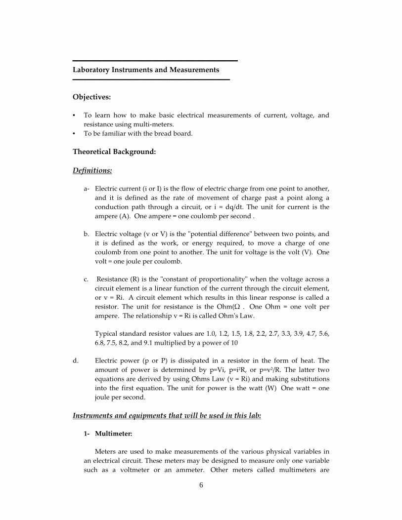
In this lab we will use a digital multimeter which is as shown in figure 1.
Figure (1) : The multimeter device
It consists of :
- Ammeter which is used to measure A.C or D.C current passing in a branch
and is connected in series with the circuit’s elements.
- Voltmeter for measuring the A.C or D.C voltage drop a cross any two point
in the circuit, and is connected in parallel.
- Ohmmeter for measuring the resistance, and is connected across the resistant.
2- Oscilloscope:
An oscilloscope (abbreviated sometimes as 'scope or O-scope) is a type of
electronic test instrument that allows signal voltages to be viewed, usually as
a two-dimensional graph which a potential differences plotted as a function
of time. Although an oscilloscope displays voltage on its vertical axis, any
other quantity that can be converted to a voltage can be displayed as well.
Oscilloscopes are commonly used when it is desired to observe the exact
wave shape of an electrical signal. In addition to the amplitude of the signal,
an oscilloscope can show distortion and measure frequency, time between
two events (such as pulse width or pulse rise time), and relative timing of two
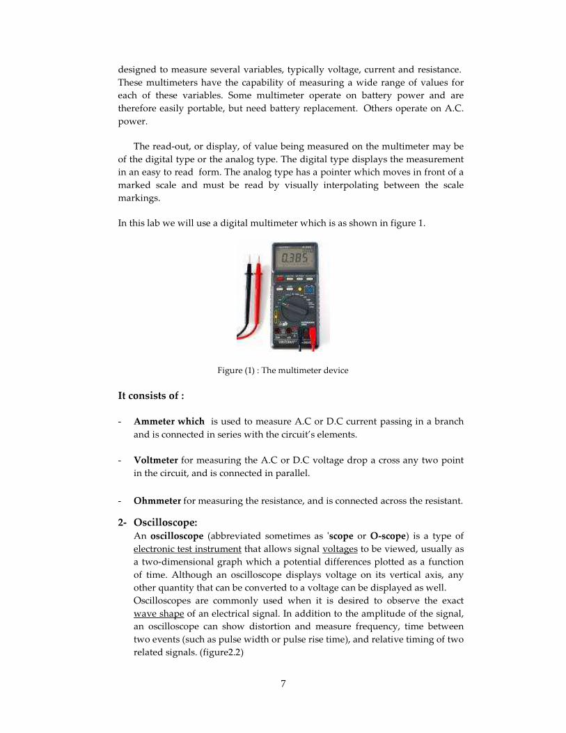
related signals. (figure2.2)
8
Figure (2) : Oscilloscope
3- Wattmeter
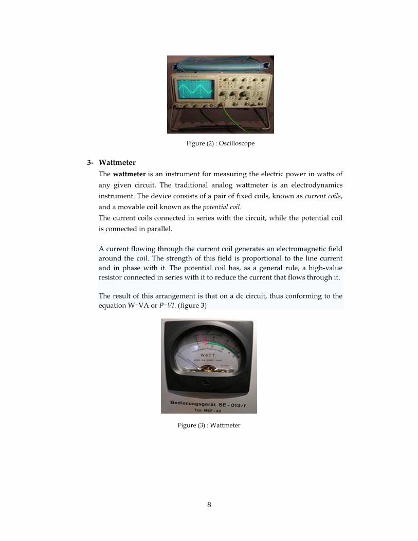
The wattmeter is an instrument for measuring the electric power in watts of
any given circuit. The traditional analog wattmeter is an electrodynamics
instrument. The device consists of a pair of fixed coils, known as current coils,
and a movable coil known as the potential coil.
The current coils connected in series with the circuit, while the potential coil
is connected in parallel.
A current flowing through the current coil generates an electromagnetic field
around the coil. The strength of this field is proportional to the line current
and in phase with it. The potential coil has, as a general rule, a high-value
resistor connected in series with it to reduce the current that flows through it.
The result of this arrangement is that on a dc circuit, thus conforming to the
equation W=VA or P=VI. (figure 3)
Figure (3) : Wattmeter
9
ـــــــــــــــــــــــــــــــــــــــــــــــــــــــــــــــــــــPrelab 1
Resistance Measurements ــــــــــــــــــــــــــــــــــــــــــــــــــــــــــــــــــــــ
a)
1- Why the voltmeter must be connected in parallel?
2- If the voltmeter is connected in series, why its reading will equal the reading
of the power supply?
3- Why the ammeter must be connected in series?
4- What is the behaviour of the capacitor and inductor at dc.?
b)
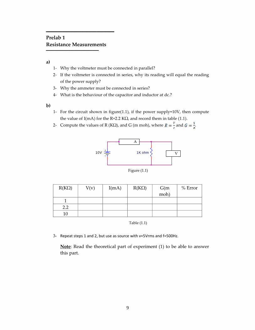
1- For the circuit shown in figure(1.1), if the power supply=10V, then compute
the value of I(mA) for the R=2.2 KΩ, and record them in table (1.1).
2- Compute the values of R (KΩ), and G (m moh), where and .
1K ohm10V
A
V
Figure (1.1)
R(KΩ) V(v) I(mA) R(KΩ) G(m
moh)
% Error
1
2.2
10
Table (1.1)
3- Repeat steps 1 and 2, but use as source with v=5Vrms and f=500Hz.
Note: Read the theoretical part of experiment (1) to be able to answer
this part.

10
c)
Figure (1.2)
Fill in the spaces:
For the circuit shown in figure (1.2)
1- Wheatstone bridge measurements method is used to measure
______________ values of resistance because _________________.
2- At stability, if R1>R3, then Runk. __________ Rvar..
3- When the readings of voltmeter is zero, if R1=R3=1KΩ, Rvar = 10KΩ, then
Runk.= _____________ .
d)
For the circuit shown in figure (1.3):
R4(unk)
R3
R1
10V
Rvar0.22 uf
1 uf10mH
A BV
Figure (1.3)
Fill in the spaces:
1- At dc, inductor acts as a ____________ and the capacitor acts as
a___________, then the circuit shown in figure (1.3) may be considered as in
figure ____________.
2- When the reading of voltmeter is zero, R1=1.8 KΩ, R3=10KΩ, Rvar.= 10KΩ
then Runk.= ___________.

11
ـــــــــــــــــــــــــــــــــــــــــــــــــــــــــــــــــــــExperiment 1
Resistance Measurements ــــــــــــــــــــــــــــــــــــــــــــــــــــــــــــــــــــــ
Part A: Familiarization
Objective:
- To measure and calculate resistors by several methods.
- Discussing the behaviour of capacitor and inductor in dc circuits.
Methods of calculating and measuring resistance:
I- By using OHM’s Law:
Experiment procedure:
a- Connect the circuit as shown in figure (1.1)
b- Set the power supply output voltage to 10v.
c- Record the value of I(ma) for R=1K, R=2.2K, and R=10K in table (1.1)
d- Compute the values of R(KΩ) using OHM Law, and G (m moh), and
compute the percentage of error for the values of R, where the
percentage of error can be computed as:
1K ohm10V
A
V
Figure(1.1)
R(KΩ) V(v) I(mA) R(KΩ) G(m
moh)
% Error
1
2.2
10 Table (1.1)
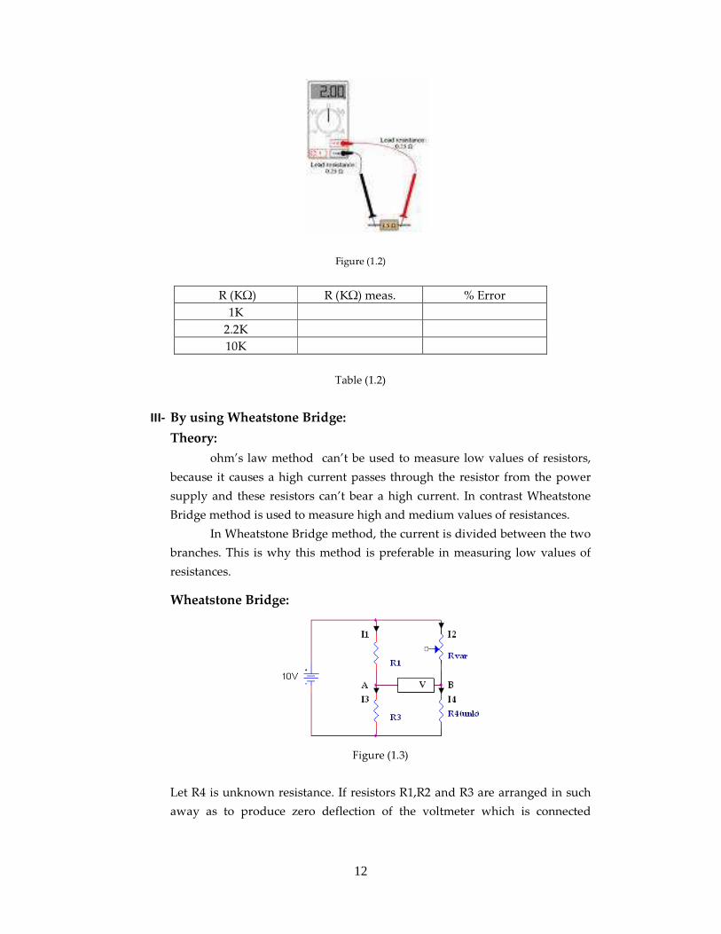
II- By using ohmmeter:
1- Connect the circuit as shown in figure (1.2).
2- Measure the value of R (KΩ) directly by connecting the digital multi-
meter in parallel with the resistor and using it as a ohmmeter.
3- Record the value of R (KΩ) and compute the percentage of error.
12
Figure (1.2)
Table (1.2)
III- By using Wheatstone Bridge:
Theory:
ohm’s law method can’t be used to measure low values of resistors,
because it causes a high current passes through the resistor from the power
supply and these resistors can’t bear a high current. In contrast Wheatstone
Bridge method is used to measure high and medium values of resistances.
In Wheatstone Bridge method, the current is divided between the two
branches. This is why this method is preferable in measuring low values of
resistances.
Wheatstone Bridge:
Figure (1.3)
Let R4 is unknown resistance. If resistors R1,R2 and R3 are arranged in such
away as to produce zero deflection of the voltmeter which is connected
R (KΩ) R (KΩ) meas. % Error
1K
2.2K
10K
13
between the points B and A, the voltage droops across R1 and R2 are equal
and the voltage drops across R3 and R4 are also equal.
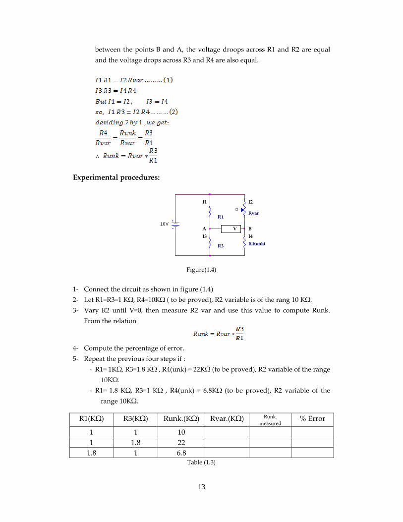
Experimental procedures:
R4(unk)R3
R1
10V
Rvar
A BV
I1 I2
I3 I4
Figure(1.4)
1- Connect the circuit as shown in figure (1.4)
2- Let R1=R3=1 KΩ, R4=10KΩ ( to be proved), R2 variable is of the rang 10 KΩ.
3- Vary R2 until V=0, then measure R2 var and use this value to compute Runk.
From the relation
4- Compute the percentage of error.
5- Repeat the previous four steps if :
- R1= 1KΩ, R3=1.8 KΩ , R4(unk) = 22KΩ (to be proved), R2 variable of the range
10KΩ.
- R1= 1.8 KΩ, R3=1 KΩ , R4(unk) = 6.8KΩ (to be proved), R2 variable of the
range 10KΩ.
R1(KΩ) R3(KΩ) Runk.(KΩ) Rvar.(KΩ) Runk.
measured % Error
1 1 10
1 1.8 22
1.8 1 6.8 Table (1.3)
14
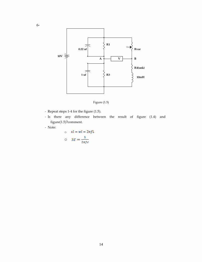
6-
R4(unk)
R3
R1
10V
Rvar0.22 uf
1 uf10mH
A BV
Figure (1.5)
- Repeat steps 1-4 for the figure (1.5).
- Is there any difference between the result of figure (1.4) and
figure(1.5)?comment.
- Note:
o
o
15
ــــــــــــــــــــــــــــــــــــــــــــــــــــــــــــــــــــــــــــــــــــــ Prelab 2
Resistor circuits and their faults ــــــــــــــــــــــــــــــــــــــــــــــــــــــــــــــــــــــــــــــــــــــ
Part A: Resistors in series and parallel:
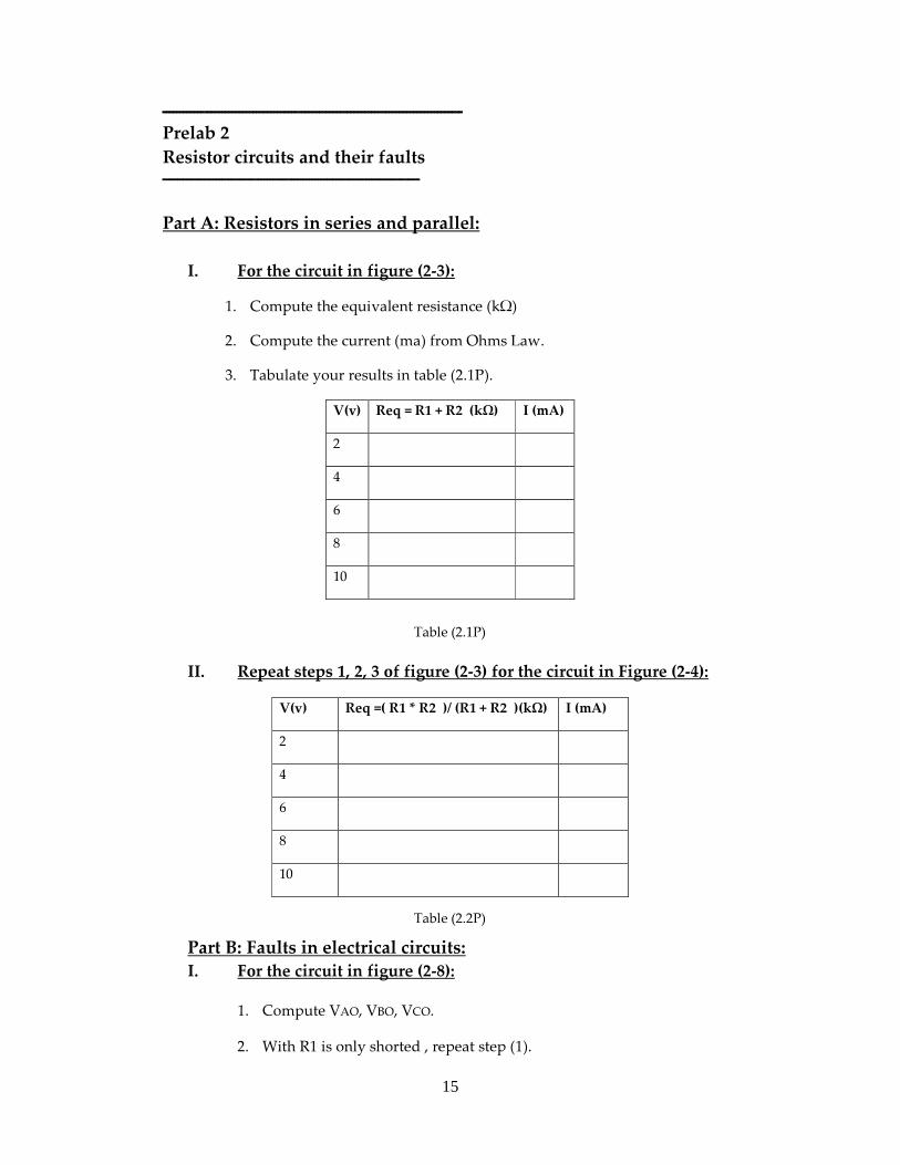
I. For the circuit in figure (2-3):
1. Compute the equivalent resistance (kΩ)
2. Compute the current (ma) from Ohms Law.
3. Tabulate your results in table (2.1P).
V(v) Req = R1 + R2 (kΩ) I (mA)
2
4
6
8
10
Table (2.1P)
II. Repeat steps 1, 2, 3 of figure (2-3) for the circuit in Figure (2-4):
V(v) Req =( R1 * R2 )/ (R1 + R2 )(kΩ) I (mA)
2
4
6
8
10
Table (2.2P)
Part B: Faults in electrical circuits:
I. For the circuit in figure (2-8):
1. Compute VAO, VBO, VCO.
2. With R1 is only shorted , repeat step (1).
16
3. With R2 is only shorted , repeat step (1).
4. With R3 is only shorted , repeat step (1).
5. With R1 is only opened , repeat step (1).
6. With R2 is only opened , repeat step (1).
7. With R3 is only opened , repeat step (1).
8. Tabulate your results in the "Calc" columns of table (2-2).
II. For the circuit of figure (2-9):
1. Compute VA, VB, and VC with respect to ground.
2. With R1 is only shorted , repeat step (1).
3. With R2 is only shorted , repeat step (1).
4. With R3 is only shorted , repeat step (1).
5. With R1 is only opened , repeat step (1).
6. With R2 is only opened , repeat step (1).
7. With R3 is only opened , repeat step (1).
8. Tabulate your results in the "Calc" columns of table (2-3).
III. For the circuit of figure (2-10):
1. Compute I, I1, I12, I2, I3.
2. With R1 is only shorted , repeat step (1).
3. With R2 is only shorted , repeat step (1).
4. With R3 is only shorted , repeat step (1).
5. With R1 is only opened , repeat step (1).
6. With R2 is only opened , repeat step (1).
7. With R3 is only opened , repeat step (1).
8. Tabulate your results in the "Calc" columns of table (2-4).
17
V Req
V Req
ـــــــــــــــــــــــــــــــــــــــــــــــــــــــــــــــــــــــــــــــــــــExperiment 2
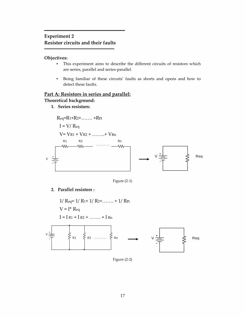
Resistor circuits and their faults ــــــــــــــــــــــــــــــــــــــــــــــــــــــــــــــــــــــــــــــــــــــ
Objectives:
• This experiment aims to describe the different circuits of resistors which
are series, parallel and series-parallel.
• Being familiar of these circuits’ faults as shorts and opens and how to
detect these faults.
Part A: Resistors in series and parallel:
Theoretical background:
1. Series resistors:
Req=R1+R2+……. +Rn
I = V/ Req
V= VR1 + VR2 + ……..+ VRn
V
R1 R2 Rn.........
Figure (2-1)
2. Parallel resistors :
1/ Req= 1/ R1+ 1/ R2+……. + 1/ Rn
V = I* Req
I = I R1 + I R2 + ……. + I Rn
VRnR2R1 .........
Figure (2-2)
18
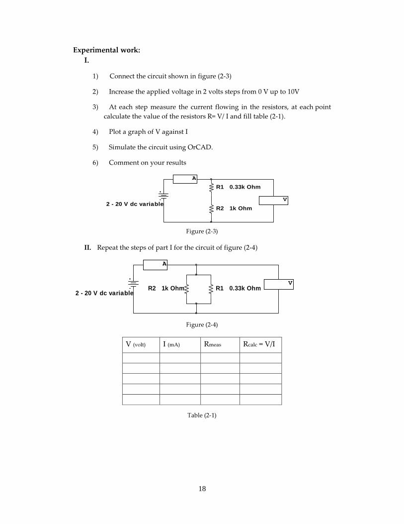
Experimental work:
I.
1) Connect the circuit shown in figure (2-3)
2) Increase the applied voltage in 2 volts steps from 0 V up to 10V
3) At each step measure the current flowing in the resistors, at each point
calculate the value of the resistors R= V/ I and fill table (2-1).
4) Plot a graph of V against I
5) Simulate the circuit using OrCAD.
6) Comment on your results
2 - 20 V dc variable
R1 0.33k Ohm
R2 1k Ohm
A
V
Figure (2-3)
II. Repeat the steps of part I for the circuit of figure (2-4)
2 - 20 V dc variableR1 0.33k OhmR2 1k Ohm
A
V
Figure (2-4)
V (volt) I (mA) Rmeas Rcalc = V/I
Table (2-1)
19
Vs R
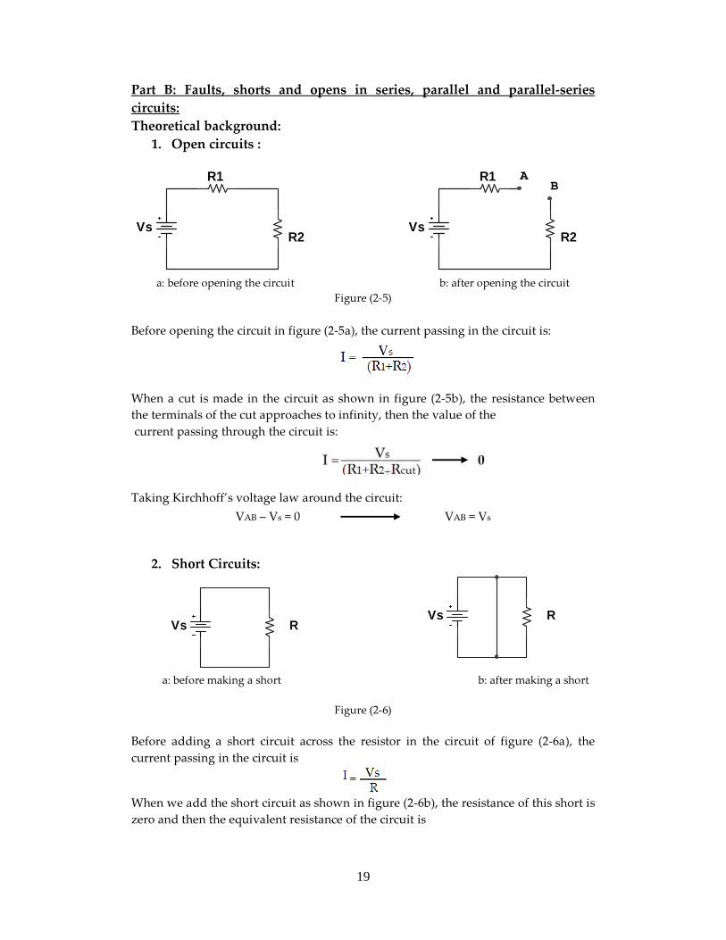
Part B: Faults, shorts and opens in series, parallel and parallel-series
circuits:
Theoretical background:
1. Open circuits :
Vs
R1
R2
Vs
R1
R2
AB
a: before opening the circuit b: after opening the circuit
Figure (2-5)
Before opening the circuit in figure (2-5a), the current passing in the circuit is:
When a cut is made in the circuit as shown in figure (2-5b), the resistance between
the terminals of the cut approaches to infinity, then the value of the
current passing through the circuit is:
Taking Kirchhoff’s voltage law around the circuit:
VAB – Vs = 0 VAB = Vs
2. Short Circuits:
Vs R
a: before making a short b: after making a short
Figure (2-6)
Before adding a short circuit across the resistor in the circuit of figure (2-6a), the
current passing in the circuit is
When we add the short circuit as shown in figure (2-6b), the resistance of this short is
zero and then the equivalent resistance of the circuit is
20
Then the value of the current passing through the circuit is
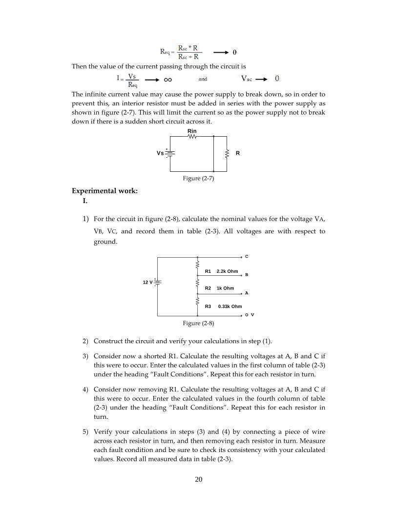
The infinite current value may cause the power supply to break down, so in order to
prevent this, an interior resistor must be added in series with the power supply as
shown in figure (2-7). This will limit the current so as the power supply not to break
down if there is a sudden short circuit across it.
Vs R
Rin
Figure (2-7)
Experimental work:
I.
1) For the circuit in figure (2-8), calculate the nominal values for the voltage VA,
VB, VC, and record them in table (2-3). All voltages are with respect to
ground.
12 V
R1 2.2k Ohm
R2 1k Ohm
R3 0.33k Ohm
A
B
C
O V Figure (2-8)
2) Construct the circuit and verify your calculations in step (1).
3) Consider now a shorted R1. Calculate the resulting voltages at A, B and C if
this were to occur. Enter the calculated values in the first column of table (2-3)
under the heading “Fault Conditions”. Repeat this for each resistor in turn.
4) Consider now removing R1. Calculate the resulting voltages at A, B and C if
this were to occur. Enter the calculated values in the fourth column of table
(2-3) under the heading “Fault Conditions”. Repeat this for each resistor in
turn.
5) Verify your calculations in steps (3) and (4) by connecting a piece of wire
across each resistor in turn, and then removing each resistor in turn. Measure
each fault condition and be sure to check its consistency with your calculated
values. Record all measured data in table (2-3).
21
6) Simulate the circuit the circuit using OrCAD.
Voltage
Normal
Short Resistors Open Resistors
R1 S/C R2 S/C R3 S/C R1 O/C R1 O/C R1 O/C
Meas Calc Meas Calc Meas Calc Meas Calc Meas Calc Meas Calc
VA
VB
VC Table (2-2)
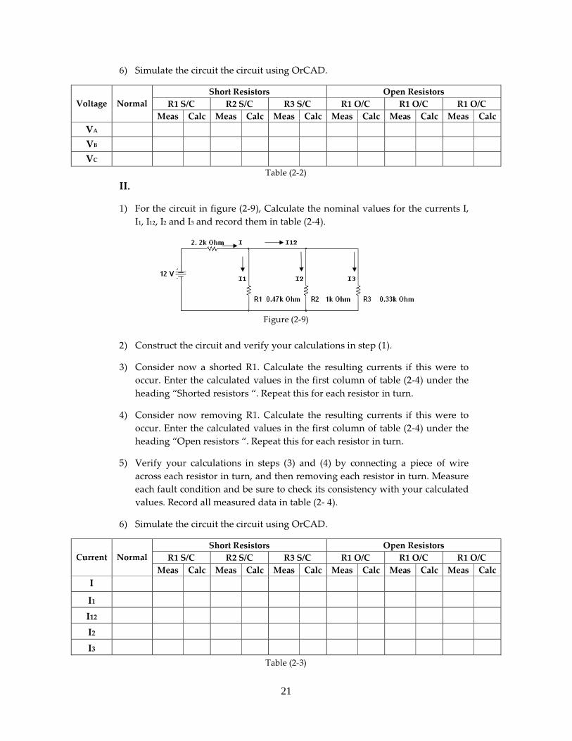
II.
1) For the circuit in figure (2-9), Calculate the nominal values for the currents I,
I1, I12, I2 and I3 and record them in table (2-4).
Figure (2-9)
2) Construct the circuit and verify your calculations in step (1).
3) Consider now a shorted R1. Calculate the resulting currents if this were to
occur. Enter the calculated values in the first column of table (2-4) under the
heading “Shorted resistors “. Repeat this for each resistor in turn.
4) Consider now removing R1. Calculate the resulting currents if this were to
occur. Enter the calculated values in the first column of table (2-4) under the
heading “Open resistors “. Repeat this for each resistor in turn.
5) Verify your calculations in steps (3) and (4) by connecting a piece of wire
across each resistor in turn, and then removing each resistor in turn. Measure
each fault condition and be sure to check its consistency with your calculated
values. Record all measured data in table (2- 4).
6) Simulate the circuit the circuit using OrCAD.
Current
Normal
Short Resistors Open Resistors
R1 S/C R2 S/C R3 S/C R1 O/C R1 O/C R1 O/C
Meas Calc Meas Calc Meas Calc Meas Calc Meas Calc Meas Calc
I
I1
I12
I2
I3
Table (2-3)

22
III.
1) For the circuit in figure (2-10), calculate the nominal values for the voltage
VA, VB, VC, and record them in table (2-5). All voltages are with respect to
ground.
12 V
R2 1k Ohm
R3 0.47k Ohm
R1 2.2k Ohm
R4 0.33k Ohm
A B C
Figure (2-10)
2) Construct the circuit and verify your calculations in step (1).
3) Consider now a shorted R1. Calculate the resulting currents if this were to
occur. Enter the calculated values in the first column of table (2-5) under the
heading “Shorted resistors “. Repeat this for each resistor in turn.
4) Consider now removing R1. Calculate the resulting currents if this were to
occur. Enter the calculated values in the first column of table (2-4) under the
heading “Open resistors “. Repeat this for each resistor in turn.
5) Verify your calculations in steps (3) and (4) by connecting a piece of wire
across each resistor in turn, and then removing each resistor in turn. Measure
each fault condition and be sure to check its consistency with your calculated
values. Record all measured data in table (2- 5).
6) Simulate the circuit the circuit using OrCAD.
Voltage
Normal
Short Resistors Open Resistors R1 S/C R2 S/C R3 S/C R1 O/C R1 O/C R1 O/C
Meas Calc Meas Calc Meas Calc Meas Calc Meas Calc Meas Calc VA VB VC
7)
Table (2-4)
23
ــــــــــــــــــــــــــــــــــ Pre-Lab 3
Oscilloscope ــــــــــــــــــــــــــــــــــ
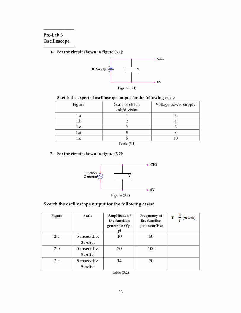
1- For the circuit shown in figure (3.1):
DC Supply V
CH1
0V Figure (3.1)
Sketch the expected oscilloscope output for the following cases:
Figure Scale of ch1 in
volt/division
Voltage power supply
1.a 1 2
1.b 2 4
1.c 2 6
1.d 5 8
1.e 5 10
Table (3.1)
2- For the circuit shown in figure (3.2):
V
CH1
0V
Function
Genertor
Figure (3.2)
Sketch the oscilloscope output for the following cases:
Figure Scale Amplitude of
the function
generator (Vp-
p)
Frequency of
the function
generator(Hz)
2.a 5 msec/div.
2v/div.
10 50
2.b 5 msec/div.
5v/div.
20 100
2.c 5 msec/div.
5v/div.
14 70
Table (3.2)
24
ـــــــــــــــــــــــــــــــــــــ
Experiment 3
Oscilloscope ــــــــــــــــــــــــــــــــــــــ
Objective:
In this experiment we shall study how to use the oscilloscope to make some
measurements in the lab.
Introduction:
We can use the oscilloscope to measure the frequency of a wave, the peak-to-peak
value, and the rms value of voltage, also to measure the phase between two waves.
Apparatus Required:
- Power supply unit.
- Function wave generator.
- Oscilloscope
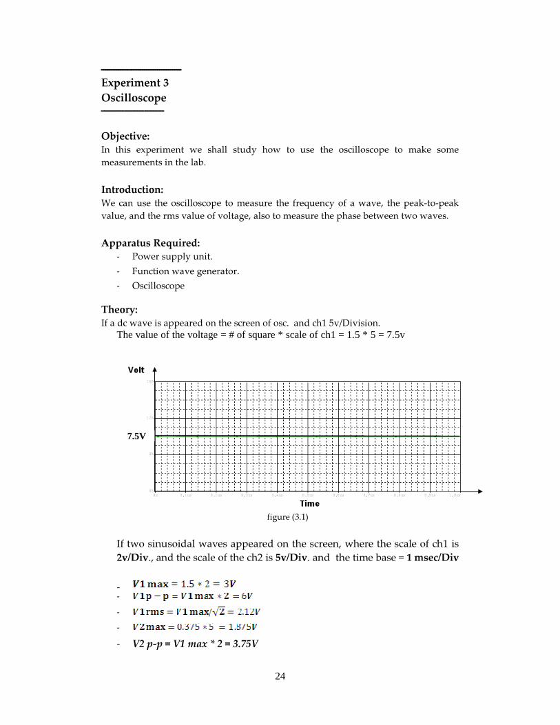
Theory:
If a dc wave is appeared on the screen of osc. and ch1 5v/Division. The value of the voltage = # of square * scale of ch1 = 1.5 * 5 = 7.5v
figure (3.1)
If two sinusoidal waves appeared on the screen, where the scale of ch1 is
2v/Div., and the scale of the ch2 is 5v/Div. and the time base = 1 msec/Div
- -
-
-
- V2 p-p = V1 max * 2 = 3.75V
7.5V
25
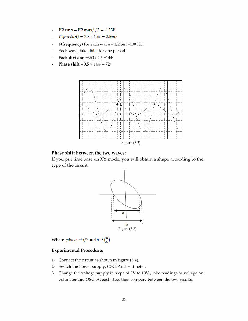
-
-
- F(frequency) for each wave = 1/2.5m =400 Hz
- Each wave take for one period.
- Each division =360 / 2.5 =144o
- Phase shift = 0.5 × 144o = 72o
Figure (3.2)
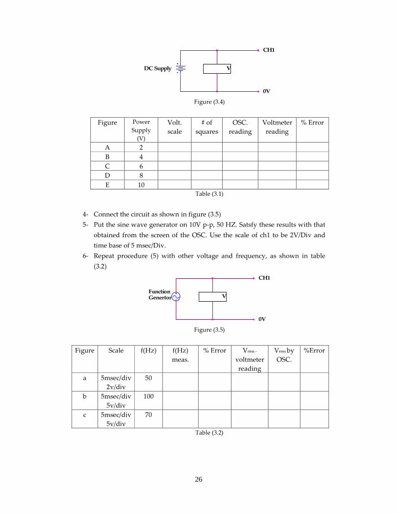
Phase shift between the two waves:
If you put time base on XY mode, you will obtain a shape according to the
type of the circuit.
Figure (3.3)
Where
Experimental Procedure:
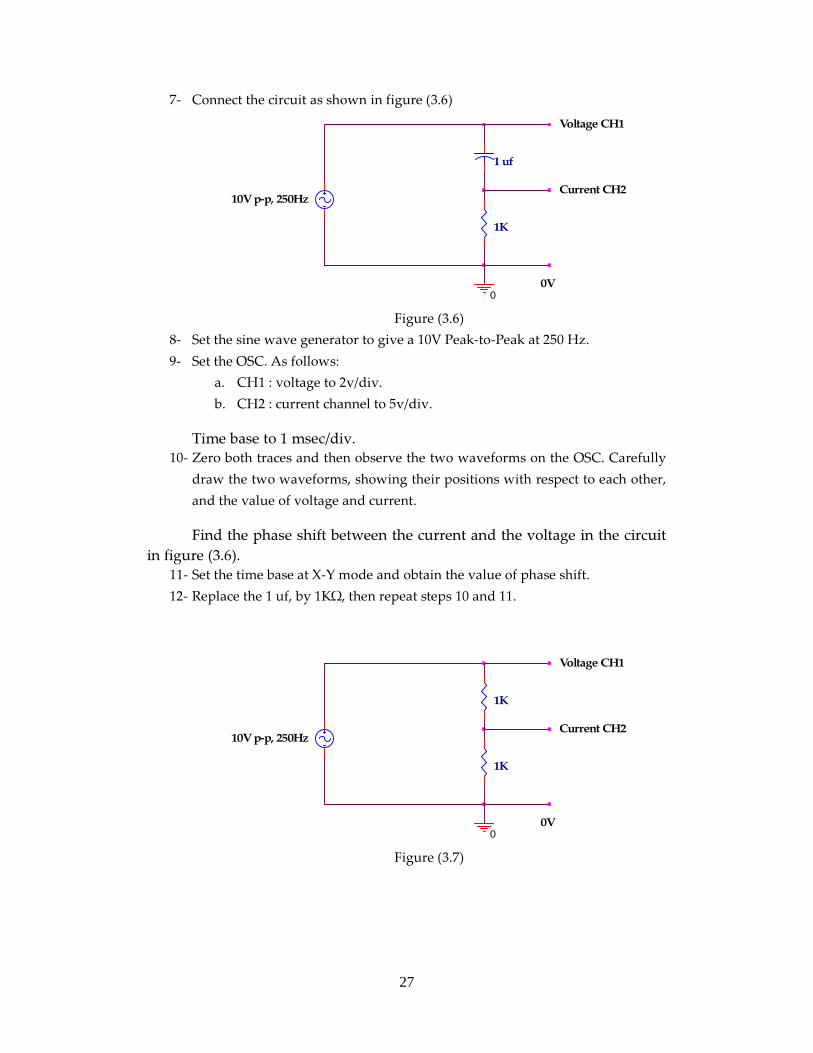
1- Connect the circuit as shown in figure (3.4).
2- Switch the Power supply, OSC. And voltmeter.
3- Change the voltage supply in steps of 2V to 10V , take readings of voltage on
voltmeter and OSC. At each step, then compare between the two results.
26
DC Supply V
CH1
0V Figure (3.4)
Figure Power
Supply
(V)
Volt.
scale
# of
squares
OSC.
reading
Voltmeter
reading
% Error
A 2
B 4
C 6
D 8
E 10
Table (3.1)
4- Connect the circuit as shown in figure (3.5)
5- Put the sine wave generator on 10V p-p, 50 HZ. Satsfy these results with that
obtained from the screen of the OSC. Use the scale of ch1 to be 2V/Div and
time base of 5 msec/Div.
6- Repeat procedure (5) with other voltage and frequency, as shown in table
(3.2)
V
CH1
0V
Function
Genertor
Figure (3.5)
Figure Scale f(Hz) f(Hz)
meas.
% Error Vrms -
voltmeter
reading
Vrms by
OSC.
%Error
a 5msec/div
2v/div
50
b 5msec/div
5v/div
100
c 5msec/div
5v/div
70
Table (3.2)
27
7- Connect the circuit as shown in figure (3.6)
0
1 uf
1K
Voltage CH1
0V
10V p-p, 250HzCurrent CH2
Figure (3.6)
8- Set the sine wave generator to give a 10V Peak-to-Peak at 250 Hz.
9- Set the OSC. As follows:
a. CH1 : voltage to 2v/div.
b. CH2 : current channel to 5v/div.
Time base to 1 msec/div.
10- Zero both traces and then observe the two waveforms on the OSC. Carefully
draw the two waveforms, showing their positions with respect to each other,
and the value of voltage and current.
Find the phase shift between the current and the voltage in the circuit
in figure (3.6).
11- Set the time base at X-Y mode and obtain the value of phase shift.
12- Replace the 1 uf, by 1KΩ, then repeat steps 10 and 11.
0
1K
1K
Voltage CH1
0V
10V p-p, 250HzCurrent CH2
Figure (3.7)
28
ـــــــــــــــــــــــــــــــــــــــــــــــــــــــــــــــــــــــــــــــــــــــــــــ Prelab 4
Millman’s and Reciprocity Theorems ـــــــــــــــــــــــــــــــــــــــــــــــــــــــــــــــــــــــــــــــــــــــــــــــــ
I. For the circuit in figure (4-7a) and figure (4-7b) :
a) Calculate :
- The voltage across the terminals A- B with the 1kΩ resistor connected.
- The current in the 1kΩ resistor.
- The voltage across the open-circuited terminals A- B after having
removed the 1kΩ resistor.
b) Using the resistor values measured in step1; compute the millman
equivalent voltage and resistance EM and RM.
c) Connect the circuit as shown in figure (4-7b). EM and RM are the values
computed n step 3.
d) Repeat step (b) for the circuit in figure (4-7b).
II. For the circuit in figure (4-8a) and figure (4-8b):
a) Calculate the currents I1, I2 and I3 flowing as shown in the figure.
b) Now connect the power supply in series with the 1.8kΩ resistor and calculate
the current I. See the figure (4-8b), and note the polarity of the relocated
power source.
c) In a similar way, relocate the power supply so that it will be in series with the
2.2kΩ and the 470Ω resistance and again calculate the current I.
29
ـــــــــــــــــــــــــــــــــــــــــــــــــــــــــــــــــــــــــــــــــــــــــــــــــــــــــــــــــــــــــــــــــــــــــــــــــــــ Experiment 4
Resistor Networks, Millman’s and Reciprocity Theorems ـــــــــــــــــــــــــــــــــــــــــــــــــــــــــــــــــــــــــــــــــــــــــــــــــــــــــــــــــــــــــــــــــــــــــــــــــــــ
Part A: Resistor Networks Objectives:
• To investigate what happens when resistor are interconnected in a circuit.
• To investigate the effect of more than one voltage source in a network.
(superposition)
• To satisfy KVL and KCL for a resistive circuit.
Theoretical Background:
The student has to study the solution of the network from any book for electric
circuit using Kirchhoff’s law (KCL and KVL) or superposition theorem.
Experimental Procedure:
I.
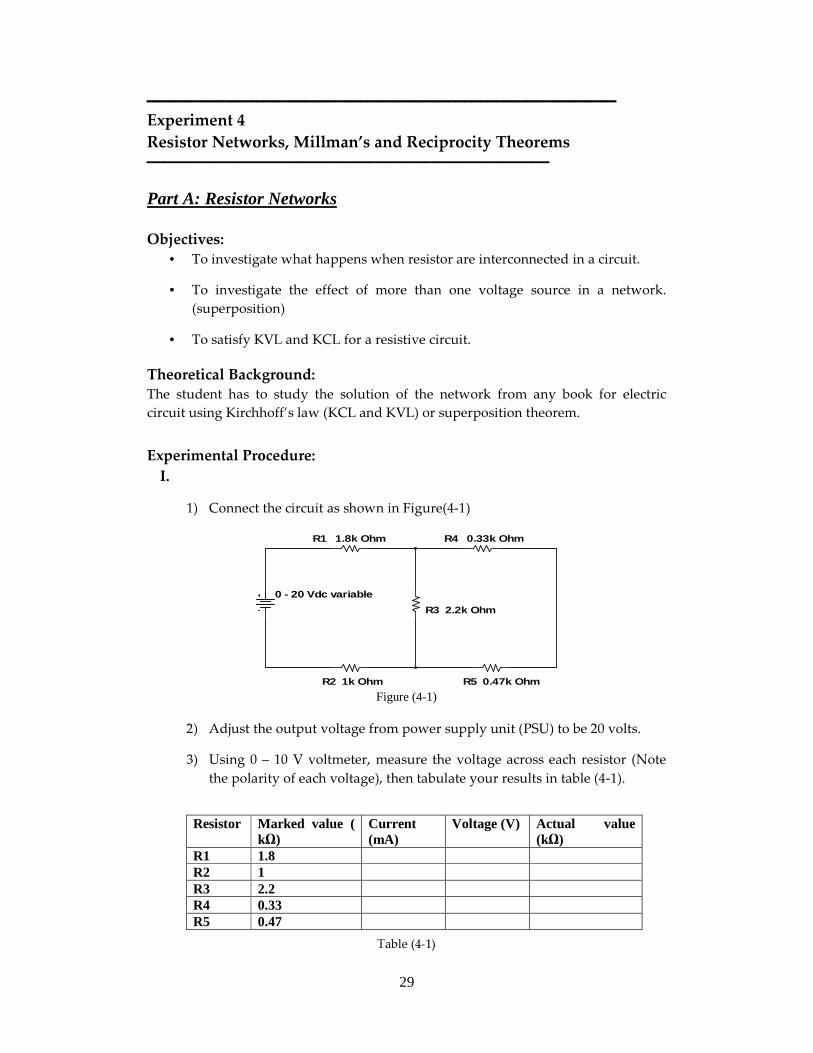
1) Connect the circuit as shown in Figure(4-1)
R1 1.8k Ohm R4 0.33k Ohm
R2 1k Ohm R5 0.47k Ohm
R3 2.2k Ohm
0 - 20 Vdc variable
Figure (4-1)
2) Adjust the output voltage from power supply unit (PSU) to be 20 volts.
3) Using 0 – 10 V voltmeter, measure the voltage across each resistor (Note
the polarity of each voltage), then tabulate your results in table (4-1).
Resistor Marked value (
kΩ) Current (mA)
Voltage (V) Actual value (kΩ)
R1 1.8 R2 1 R3 2.2 R4 0.33 R5 0.47
Table (4-1)
30
4) Measure the current in each component using the multi-meter then
tabulate your results in table (4-1).
5) From the measured values of current and voltage in each branch, calculate
using ohms law the value of the resistance in each leg of the network, and
copy the results in table (4-1)
6) Solve the circuit using node voltage method and mesh current method,
and compare the results.
7) Simulate the circuit using OrCAD.
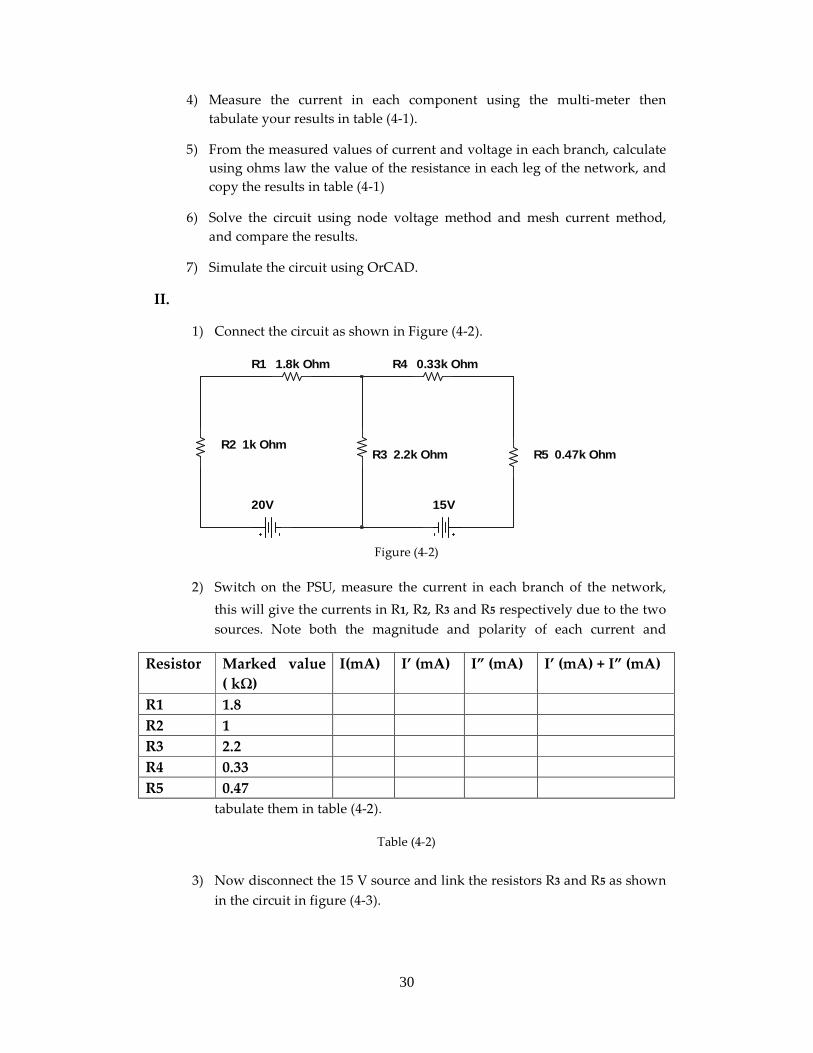
II.
1) Connect the circuit as shown in Figure (4-2).
R1 1.8k Ohm R4 0.33k Ohm
R5 0.47k OhmR3 2.2k Ohm
20V
R2 1k Ohm
15V
Figure (4-2)
2) Switch on the PSU, measure the current in each branch of the network,
this will give the currents in R1, R2, R3 and R5 respectively due to the two
sources. Note both the magnitude and polarity of each current and
tabulate them in table (4-2).
Table (4-2)
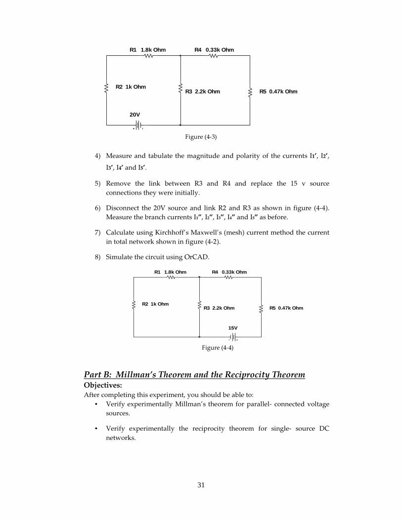
3) Now disconnect the 15 V source and link the resistors R3 and R5 as shown
in the circuit in figure (4-3).
Resistor Marked value
( kΩ)
I(mA) I’ (mA) I” (mA) I’ (mA) + I” (mA)
R1 1.8
R2 1
R3 2.2
R4 0.33
R5 0.47
31
R1 1.8k Ohm R4 0.33k Ohm
R5 0.47k OhmR3 2.2k Ohm
20V
R2 1k Ohm
Figure (4-3)
4) Measure and tabulate the magnitude and polarity of the currents I1’, I2’,
I3’, I4’ and I5’.
5) Remove the link between R3 and R4 and replace the 15 v source
connections they were initially.
6) Disconnect the 20V source and link R2 and R3 as shown in figure (4-4).
Measure the branch currents I1”, I2”, I3”, I4” and I5” as before.
7) Calculate using Kirchhoff’s Maxwell’s (mesh) current method the current
in total network shown in figure (4-2).
8) Simulate the circuit using OrCAD.
R1 1.8k Ohm R4 0.33k Ohm
R5 0.47k OhmR3 2.2k OhmR2 1k Ohm
15V
Figure (4-4)
Part B: Millman’s Theorem and the Reciprocity Theorem Objectives:
After completing this experiment, you should be able to:
• Verify experimentally Millman’s theorem for parallel- connected voltage
sources.
• Verify experimentally the reciprocity theorem for single- source DC
networks.
32
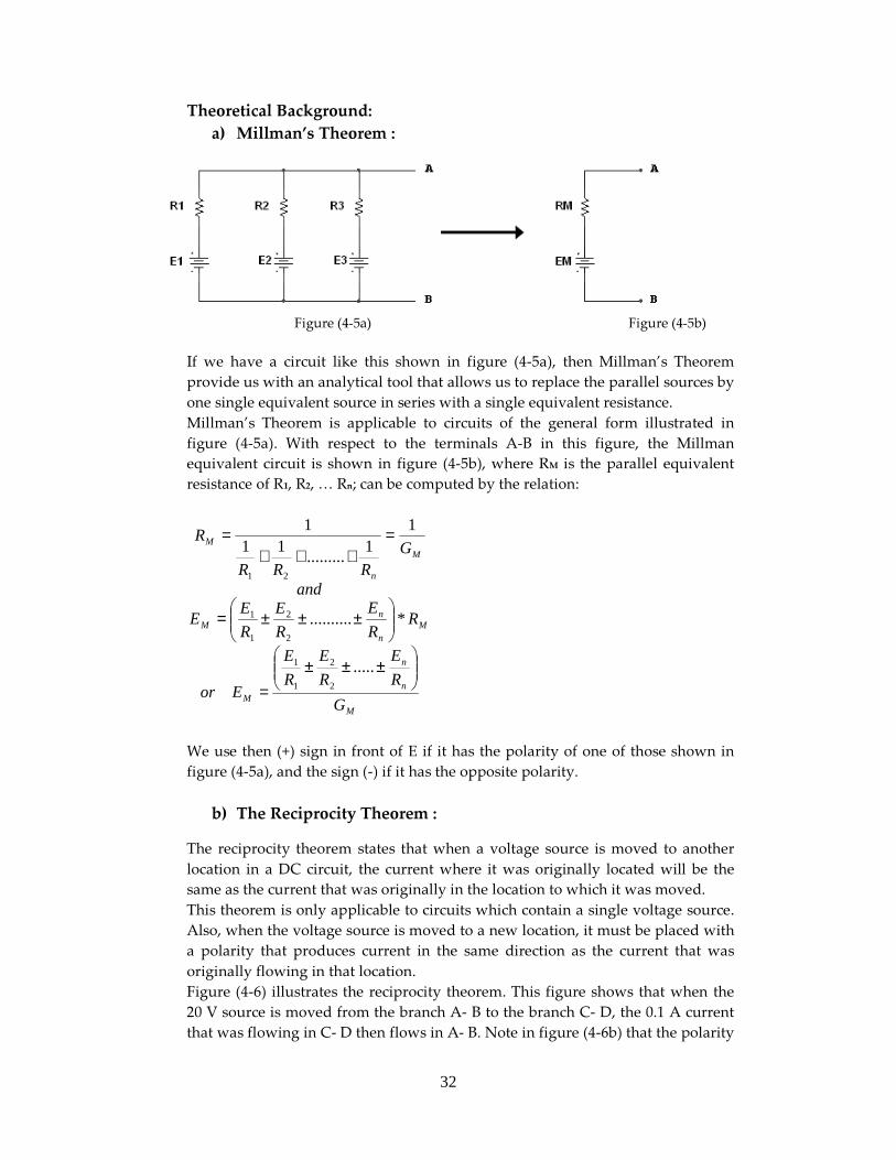
Theoretical Background:
a) Millman’s Theorem :
Figure (4-5a) Figure (4-5b)
If we have a circuit like this shown in figure (4-5a), then Millman’s Theorem
provide us with an analytical tool that allows us to replace the parallel sources by
one single equivalent source in series with a single equivalent resistance.
Millman’s Theorem is applicable to circuits of the general form illustrated in
figure (4-5a). With respect to the terminals A-B in this figure, the Millman
equivalent circuit is shown in figure (4-5b), where RM is the parallel equivalent
resistance of R1, R2, … Rn; can be computed by the relation:
M
n
n
M
Mn
nM
M
n
M
G
R
E
R
E
R
E
Eor
RR
E
R
E
R
EE
and
GRRR
R
±±±
=
±±±=
=+++
=
.....
*..........
11
.........11
1
2
2
1
1
2
2
1
1
21
We use then (+) sign in front of E if it has the polarity of one of those shown in
figure (4-5a), and the sign (-) if it has the opposite polarity.
b) The Reciprocity Theorem :
The reciprocity theorem states that when a voltage source is moved to another
location in a DC circuit, the current where it was originally located will be the
same as the current that was originally in the location to which it was moved.
This theorem is only applicable to circuits which contain a single voltage source.
Also, when the voltage source is moved to a new location, it must be placed with
a polarity that produces current in the same direction as the current that was
originally flowing in that location.
Figure (4-6) illustrates the reciprocity theorem. This figure shows that when the
20 V source is moved from the branch A- B to the branch C- D, the 0.1 A current
that was flowing in C- D then flows in A- B. Note in figure (4-6b) that the polarity
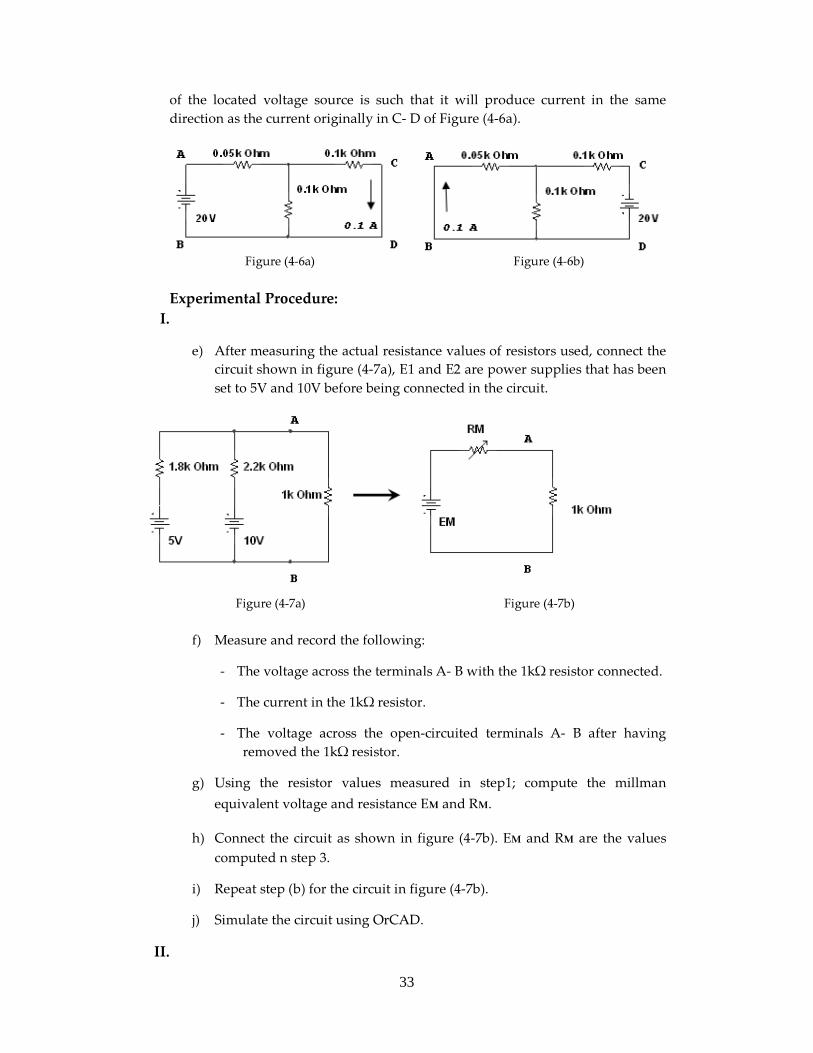
33
of the located voltage source is such that it will produce current in the same
direction as the current originally in C- D of Figure (4-6a).
Figure (4-6a) Figure (4-6b)
Experimental Procedure:
I.
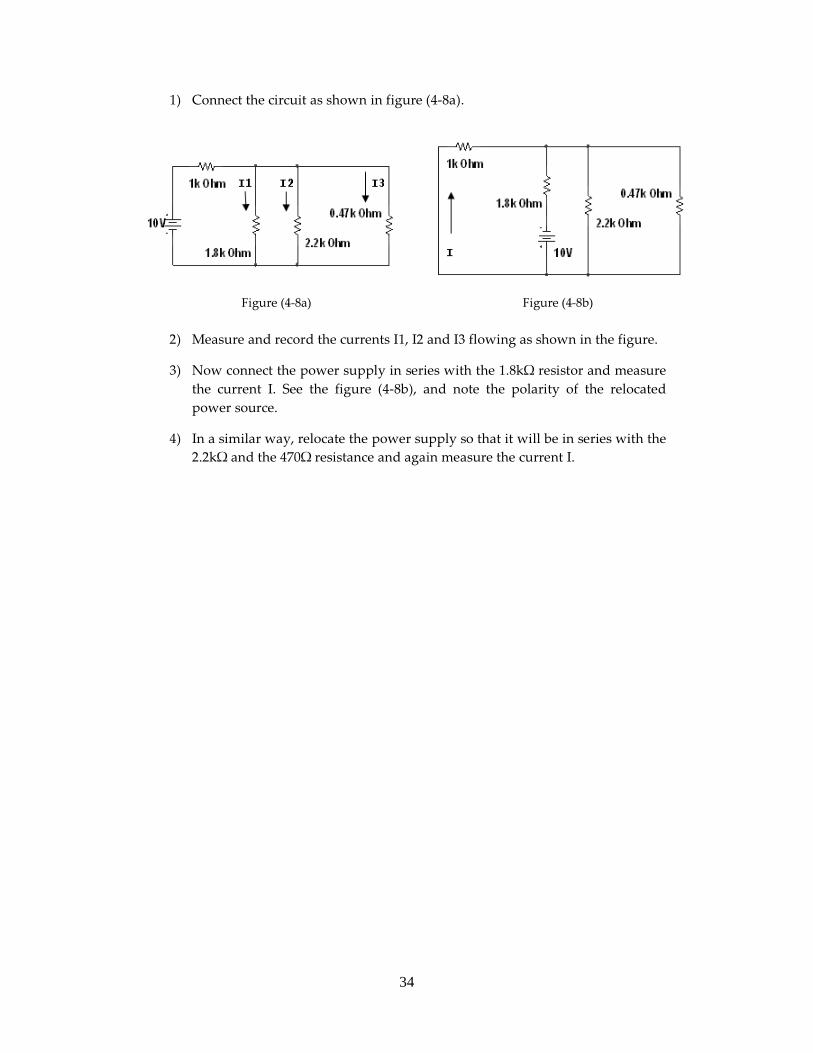
e) After measuring the actual resistance values of resistors used, connect the
circuit shown in figure (4-7a), E1 and E2 are power supplies that has been
set to 5V and 10V before being connected in the circuit.
Figure (4-7a) Figure (4-7b)
f) Measure and record the following:
- The voltage across the terminals A- B with the 1kΩ resistor connected.
- The current in the 1kΩ resistor.
- The voltage across the open-circuited terminals A- B after having
removed the 1kΩ resistor.
g) Using the resistor values measured in step1; compute the millman
equivalent voltage and resistance EM and RM.
h) Connect the circuit as shown in figure (4-7b). EM and RM are the values
computed n step 3.
i) Repeat step (b) for the circuit in figure (4-7b).
j) Simulate the circuit using OrCAD.
II.
34
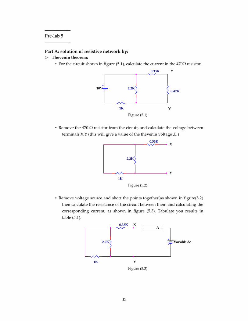
1) Connect the circuit as shown in figure (4-8a).
Figure (4-8a) Figure (4-8b)
2) Measure and record the currents I1, I2 and I3 flowing as shown in the figure.
3) Now connect the power supply in series with the 1.8kΩ resistor and measure
the current I. See the figure (4-8b), and note the polarity of the relocated
power source.
4) In a similar way, relocate the power supply so that it will be in series with the
2.2kΩ and the 470Ω resistance and again measure the current I.
35
ــــــــــــــــــــــــــــPre-lab 5 ــــــــــــــــــــــــــــ
Part A: solution of resistive network by:
1- Thevenin theorem:
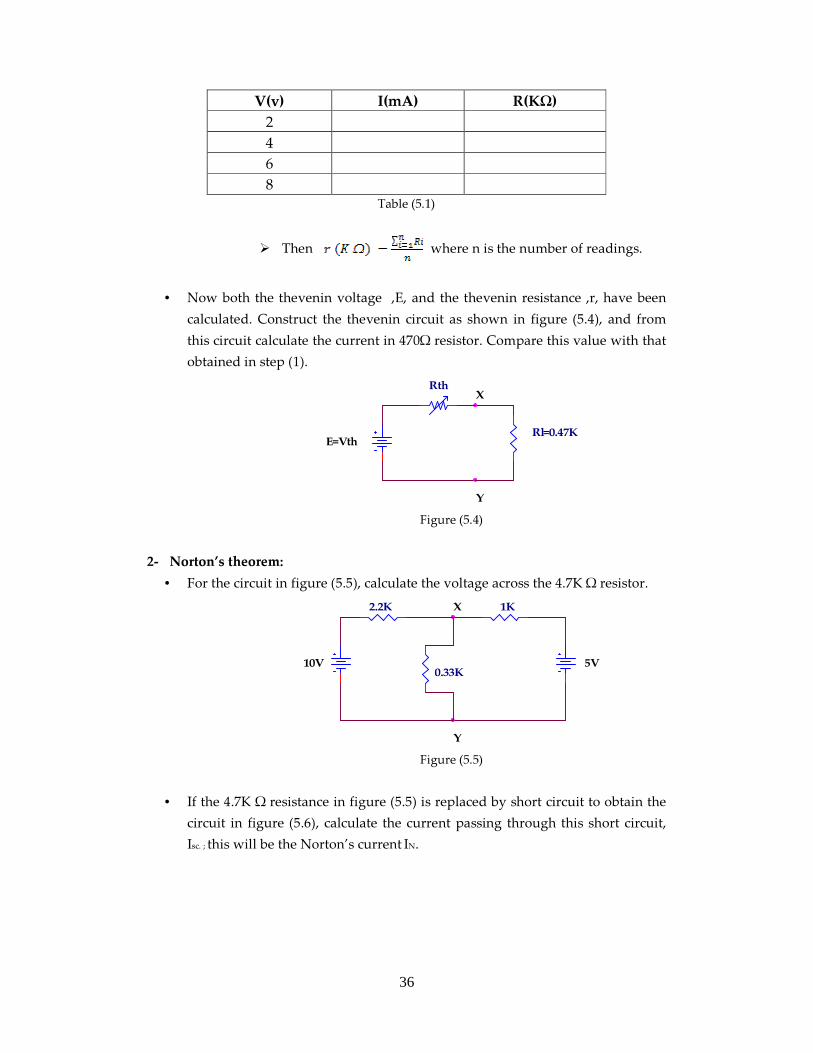
• For the circuit shown in figure (5.1), calculate the current in the 470Ω resistor.
0.33K
2.2K
1K
0.47K10V
Figure (5.1)
• Remove the 470 Ω resistor from the circuit, and calculate the voltage between
terminals X,Y (this will give a value of the thevenin voltage ,E,)
0.33K
2.2K
1K
X
Y
Figure (5.2)
• Remove voltage source and short the points together(as shown in figure(5.2)
then calculate the resistance of the circuit between them and calculating the
corresponding current, as shown in figure (5.3). Tabulate you results in
table (5.1).
0.33K
2.2K
1K
Variable dc
X
Y
A
Figure (5.3)
X
Y
36
V(v) I(mA) R(KΩ)
2
4
6
8 Table (5.1)
Then where n is the number of readings.
• Now both the thevenin voltage ,E, and the thevenin resistance ,r, have been
calculated. Construct the thevenin circuit as shown in figure (5.4), and from
this circuit calculate the current in 470Ω resistor. Compare this value with that
obtained in step (1).
Rl=0.47KE=Vth
RthX
Y Figure (5.4)
2- Norton’s theorem:
• For the circuit in figure (5.5), calculate the voltage across the 4.7K Ω resistor.
2.2K
10V
1K
0.33K5V
X
Y Figure (5.5)
• If the 4.7K Ω resistance in figure (5.5) is replaced by short circuit to obtain the
circuit in figure (5.6), calculate the current passing through this short circuit,
Isc. ; this will be the Norton’s current IN.
37
2.2K
10V
1K
5V
X
Y
A
Figure (5.6)
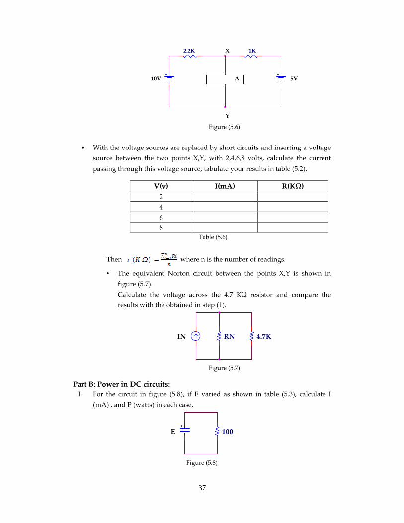
• With the voltage sources are replaced by short circuits and inserting a voltage
source between the two points X,Y, with 2,4,6,8 volts, calculate the current
passing through this voltage source, tabulate your results in table (5.2).
V(v) I(mA) R(KΩ)
2
4
6
8 Table (5.6)
Then where n is the number of readings.
• The equivalent Norton circuit between the points X,Y is shown in
figure (5.7).
Calculate the voltage across the 4.7 KΩ resistor and compare the
results with the obtained in step (1).
RN 4.7KIN
Figure (5.7)
Part B: Power in DC circuits:
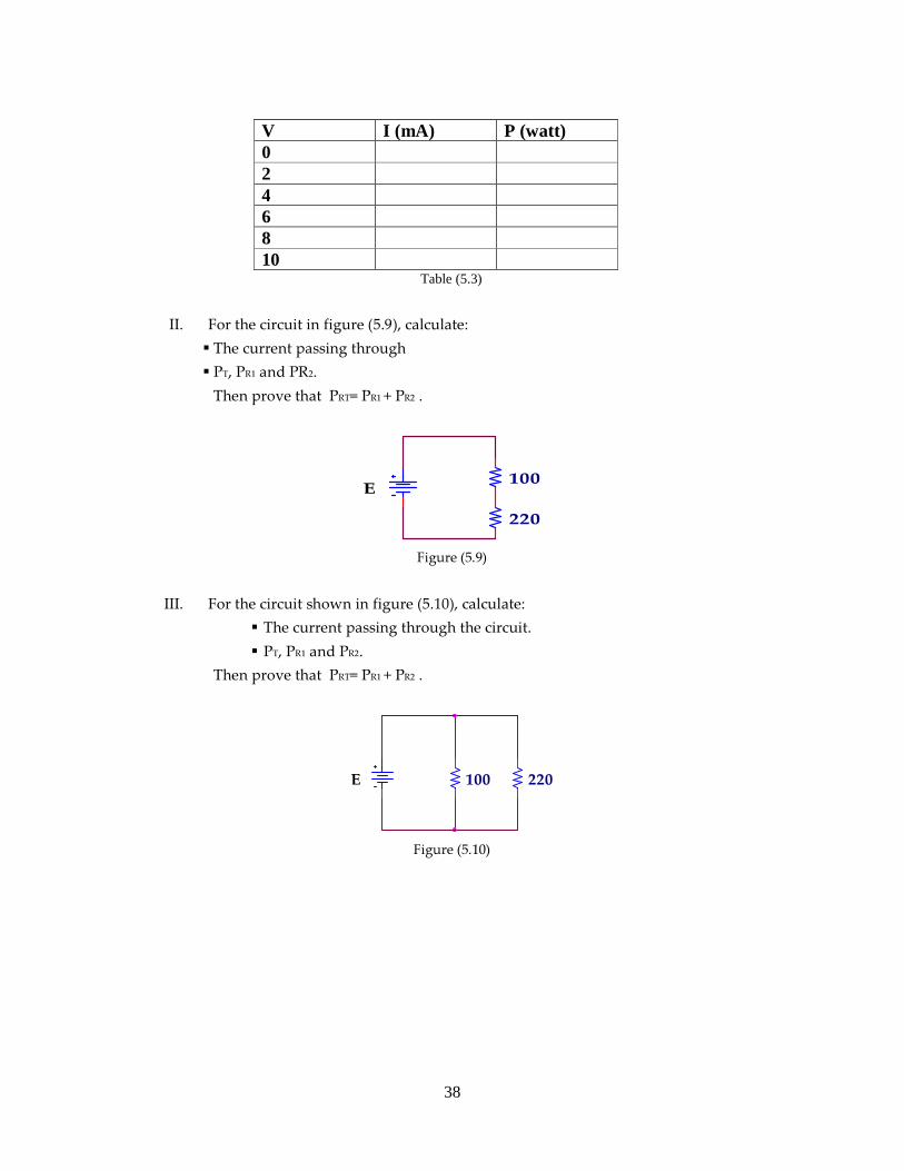
I. For the circuit in figure (5.8), if E varied as shown in table (5.3), calculate I
(mA) , and P (watts) in each case.
100E
Figure (5.8)
38
II. For the circuit in figure (5.9), calculate:
The current passing through
PT, PR1 and PR2.
Then prove that PRT= PR1 + PR2 .
100
220
E
Figure (5.9)
III. For the circuit shown in figure (5.10), calculate:
The current passing through the circuit.
PT, PR1 and PR2.
Then prove that PRT= PR1 + PR2 .
100 220E
Figure (5.10)
V I (mA) P (watt) 0 2 4 6 8 10
Table (5.3)
39
ــــــــــــــــــــــــــــــــــــــــــــــــــــــــــــــــــــــــــــــــــــــExperiment 5
A: Solution of a resistive network
B: Power in DC circuit ــــــــــــــــــــــــــــــــــــــــــــــــــــــــــــــــــــــــــــــــــــــــ
Part A: The solution of a resistive network using:
- The’venin Theorem
- Norton Theorem
Objective:
To find a method of simplifying a network in order to obtain the current
flowing in one particular branch of the network.
Theory:
The’venin’s theorem states that: the current through a resistor R connected
across any two points X and Y of a network containing one or more sources of emf is
obtained by dividing the P.d between X and Y, with R disconnected by (R+r), where r
is the resistance of the network measured between the points X and Y with R
disconnected and sources of emf replaced by their internal resistance.
Experimental Procedure:
I. Solution of the network using The’venin’s theorem:
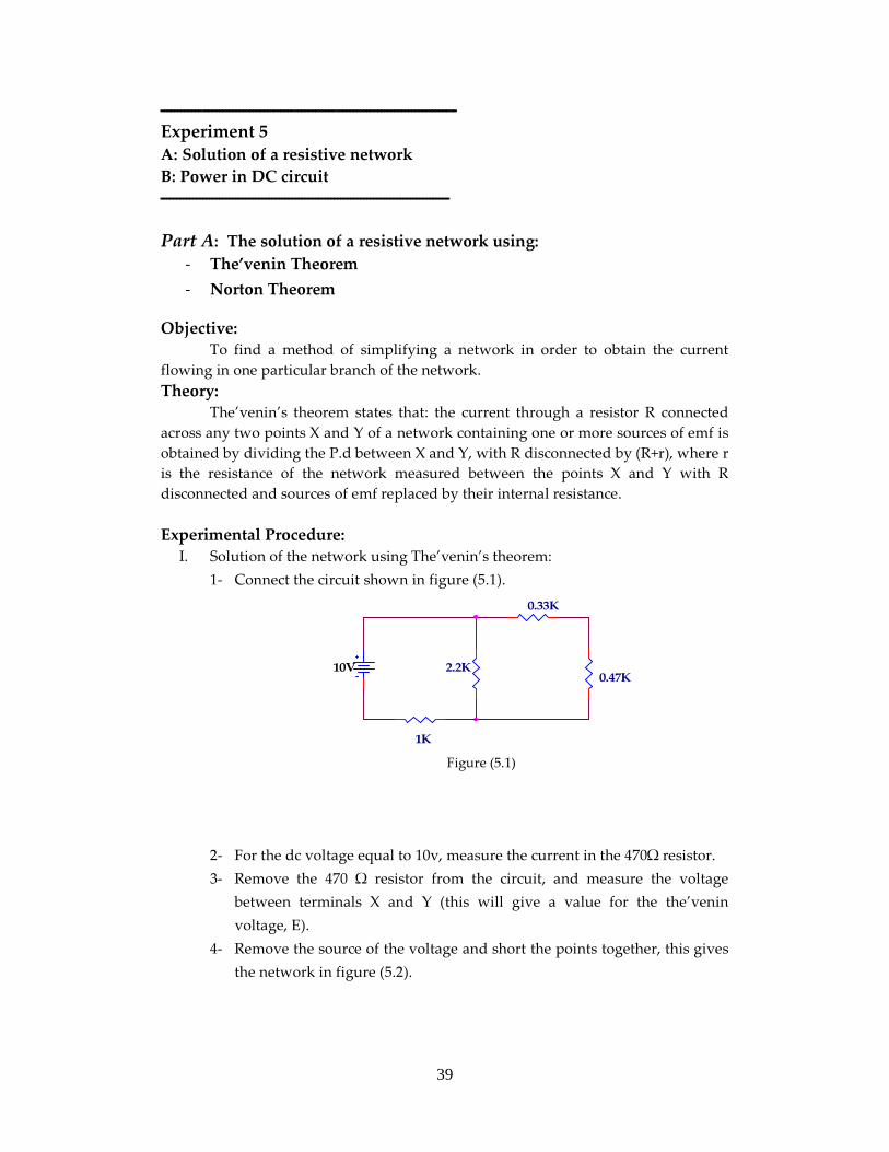
1- Connect the circuit shown in figure (5.1).
0.33K
2.2K
1K
0.47K10V
Figure (5.1)
2- For the dc voltage equal to 10v, measure the current in the 470Ω resistor.
3- Remove the 470 Ω resistor from the circuit, and measure the voltage
between terminals X and Y (this will give a value for the the’venin
voltage, E).
4- Remove the source of the voltage and short the points together, this gives
the network in figure (5.2).

40
0.33K
2.2K
1K
X
Y
Figure (5.2)
5- The resistance of this network may be found by connecting a voltage to
points X,Y and measuring the total current as shown in figure (5.2).
Measure the current for voltages of 2,4,6 and 8 Volts and tabulate your
results in table(5.1), then calculate the resistance using Ohm’s law and
take the average of r.
0.33K
2.2K
1K
Variable dc
X
Y
A
Figure (5.3)
V(v) I(mA) R(KΩ)
2
4
6
8 Table (5.1)
6- Thus we have now found the values of E and r, and a circuit shown in
figure (5.1) is simplified to the circuit shown in figure (5.4).
Rl=0.47KE=Vth
RthX
Y Figure(5.4)
41
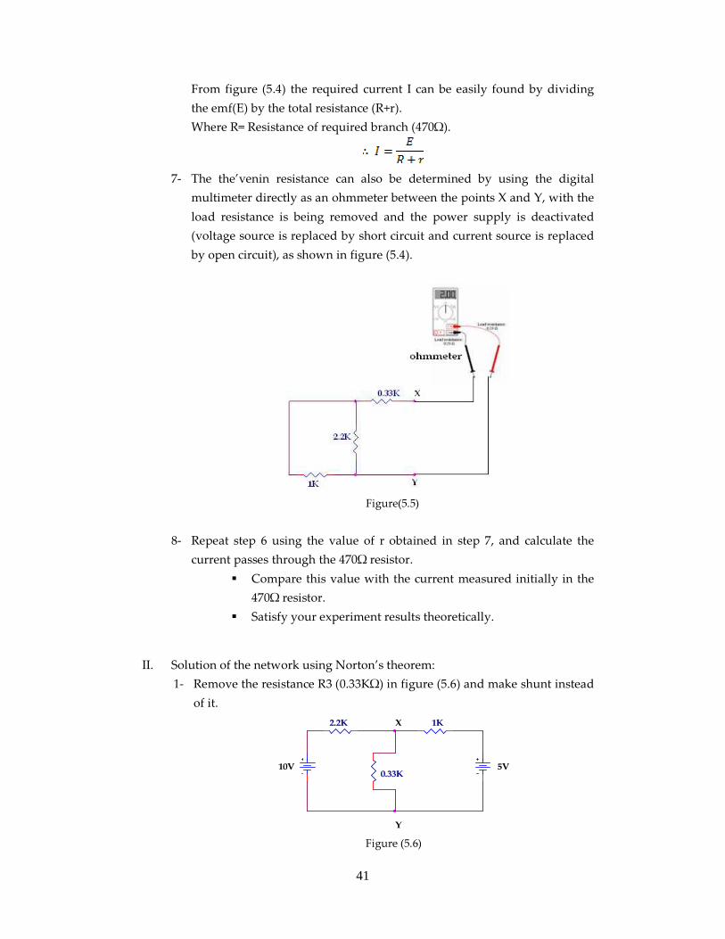
From figure (5.4) the required current I can be easily found by dividing
the emf(E) by the total resistance (R+r).
Where R= Resistance of required branch (470Ω).
7- The the’venin resistance can also be determined by using the digital
multimeter directly as an ohmmeter between the points X and Y, with the
load resistance is being removed and the power supply is deactivated
(voltage source is replaced by short circuit and current source is replaced
by open circuit), as shown in figure (5.4).
Figure(5.5)
8- Repeat step 6 using the value of r obtained in step 7, and calculate the
current passes through the 470Ω resistor.
Compare this value with the current measured initially in the
470Ω resistor.
Satisfy your experiment results theoretically.
II. Solution of the network using Norton’s theorem:
1- Remove the resistance R3 (0.33KΩ) in figure (5.6) and make shunt instead
of it.
2.2K
10V
1K
0.33K5V
X
Y Figure (5.6)
42
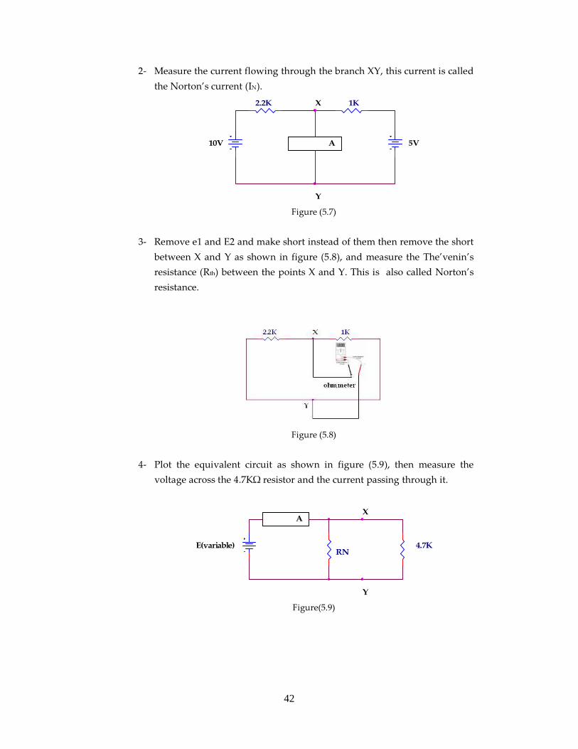
2- Measure the current flowing through the branch XY, this current is called
the Norton’s current (IN).
2.2K
10V
1K
5V
X
Y
A
Figure (5.7)
3- Remove e1 and E2 and make short instead of them then remove the short
between X and Y as shown in figure (5.8), and measure the The’venin’s
resistance (Rth) between the points X and Y. This is also called Norton’s
resistance.
Figure (5.8)
4- Plot the equivalent circuit as shown in figure (5.9), then measure the
voltage across the 4.7KΩ resistor and the current passing through it.
4.7KRN
E(variable)
X
Y
A
Figure(5.9)
43
Part B: Power in Dc Circuits:
Objective:
To investigate the concepts of electrical dc, power transfer, and the
power dissipated at dc by various components.
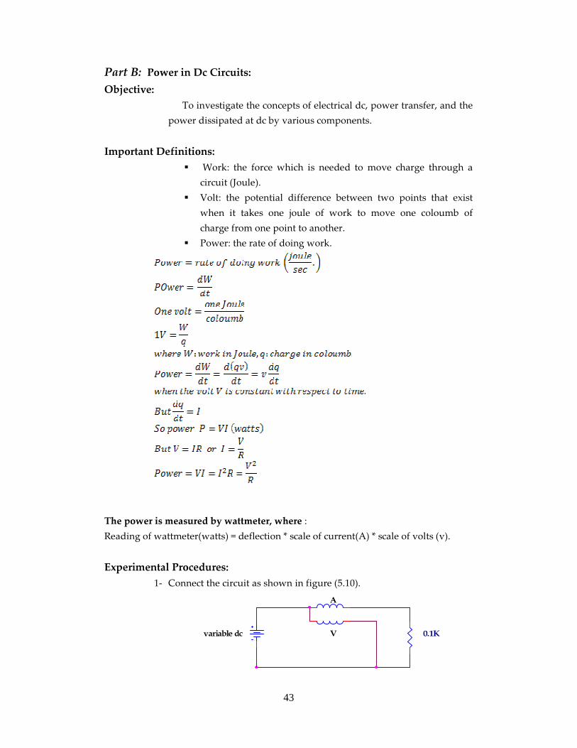
Important Definitions:
Work: the force which is needed to move charge through a
circuit (Joule).
Volt: the potential difference between two points that exist
when it takes one joule of work to move one coloumb of
charge from one point to another.
Power: the rate of doing work.
The power is measured by wattmeter, where :
Reading of wattmeter(watts) = deflection * scale of current(A) * scale of volts (v).
Experimental Procedures:
1- Connect the circuit as shown in figure (5.10).
0.1Kvariable dc
A
V
44
Figure (5.10)
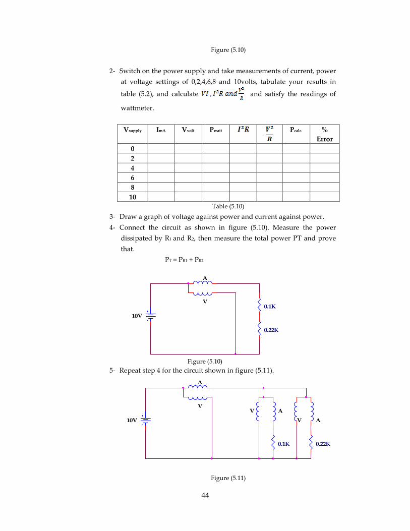
2- Switch on the power supply and take measurements of current, power
at voltage settings of 0,2,4,6,8 and 10volts, tabulate your results in
table (5.2), and calculate and satisfy the readings of
wattmeter.
Vsupply ImA Vvolt Pwatt
Pcalc. %
Error
0
2
4
6
8
10
Table (5.10)
3- Draw a graph of voltage against power and current against power.
4- Connect the circuit as shown in figure (5.10). Measure the power
dissipated by R1 and R2, then measure the total power PT and prove
that.
PT = PR1 + PR2
0.1K
0.22K
10V
A
V
Figure (5.10)
5- Repeat step 4 for the circuit shown in figure (5.11).
10V
0.22K0.1K
A
VA
A
V
V
Figure (5.11)

45
ـــــــــــــــــــــــــــــPrelab 6 ــــــــــــــــــــــــــــــ A: Electromotive Force (emf) and internal resistance of voltage source, and
maximum power transfer:
For the circuit in figure (6-1), if RL varies then I-1 will also vary according to the
relation:
Where Rin s the internal resistance of the voltage supply in this circuit, and it could
be considered, in general, as the thevenin equivalent resistance of the circuit.
Depending on the last note, obtain a similar relation I-1 and RL for the circuit in
figure (6-2)
- Discuss how do you compute the values of the electromotive force (emf) and
internal resistance of the voltage supply (Rin) for the circuit in figure (6-2)?
B: Star/ Data Conversion:
1. For the circuit in figure (6-3), find RAB, RBC, and RCA using Y/ Δ
transformation.
2. Repeat step (1) for the circuit in figure (6-4).
46
ــــــــــــــــــــــــــــــــــــــــــــــــــــــــــــــــــــــــــــــــــــــــــــــــــــــــــــــــــــــــــــــــــــــــــــــــــــــــــــــــــــــــــــــ
Experiment 6
A: Electromotive Force (emf) and internal resistance of voltage source
B: Maximum power transfer
C: Star/ Data Conversion ـــــــــــــــــــــــــــــــــــــــــــــــــــــــــــــــــــــــــــــــــــــــــــــــــــــــــــــــــــــــــــــــــــــــــــــــــــــــــــــــــــــــــــــــ
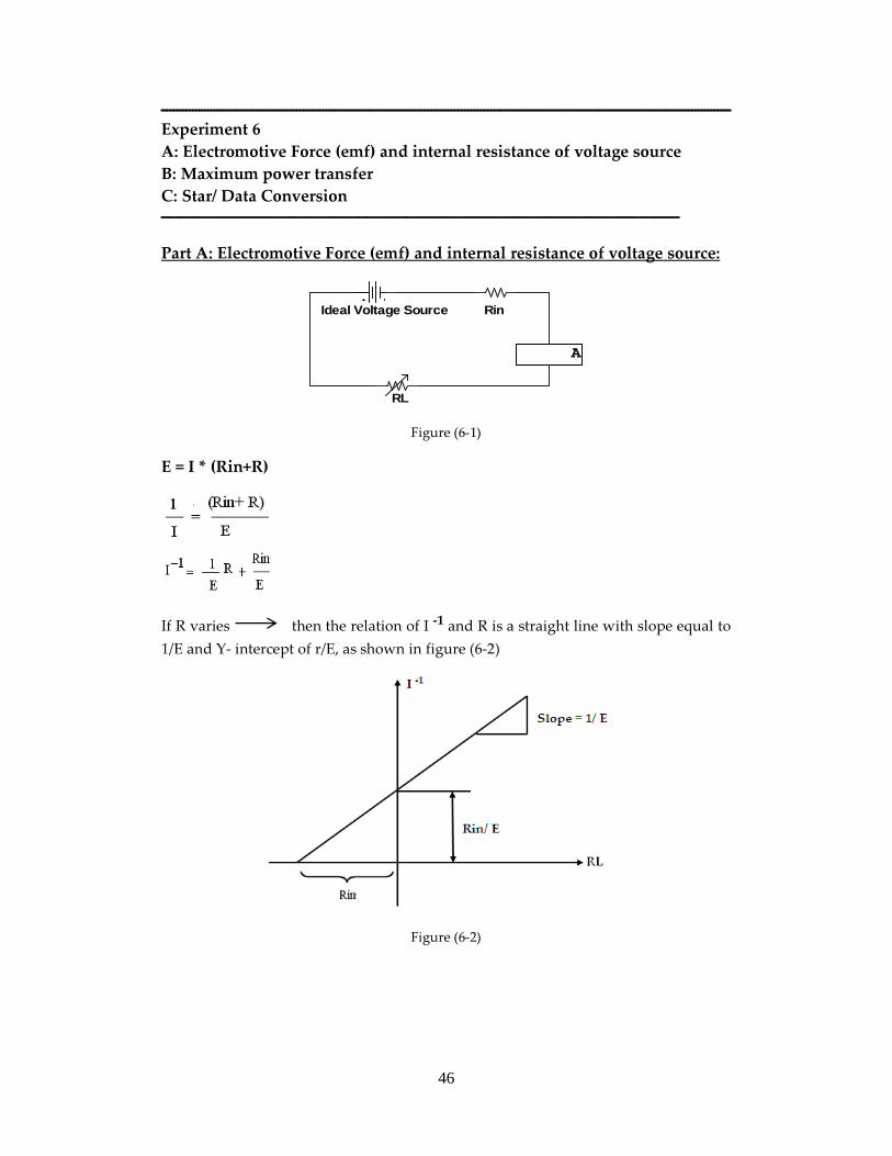
Part A: Electromotive Force (emf) and internal resistance of voltage source:
Rin
RL
Ideal Voltage Source
A
Figure (6-1)
E = I * (Rin+R)
If R varies then the relation of I -1 and R is a straight line with slope equal to
1/E and Y- intercept of r/E, as shown in figure (6-2)
Figure (6-2)
47
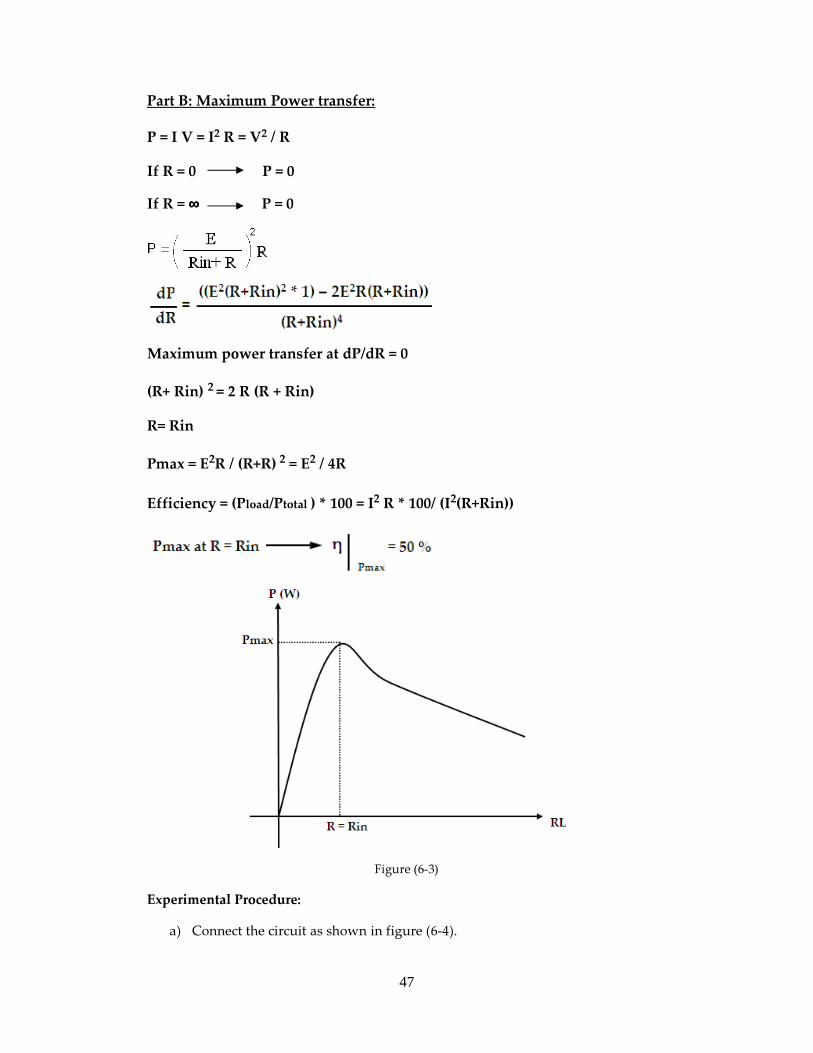
Part B: Maximum Power transfer:
P = I V = I2 R = V2 / R
If R = 0 P = 0
If R = ∞∞∞∞ P = 0
Maximum power transfer at dP/dR = 0
(R+ Rin) 2 = 2 R (R + Rin)
R= Rin
Pmax = E2R / (R+R) 2 = E2 / 4R
Efficiency = (Pload/Ptotal ) * 100 = I2 R * 100/ (I2(R+Rin))
Figure (6-3)
Experimental Procedure:
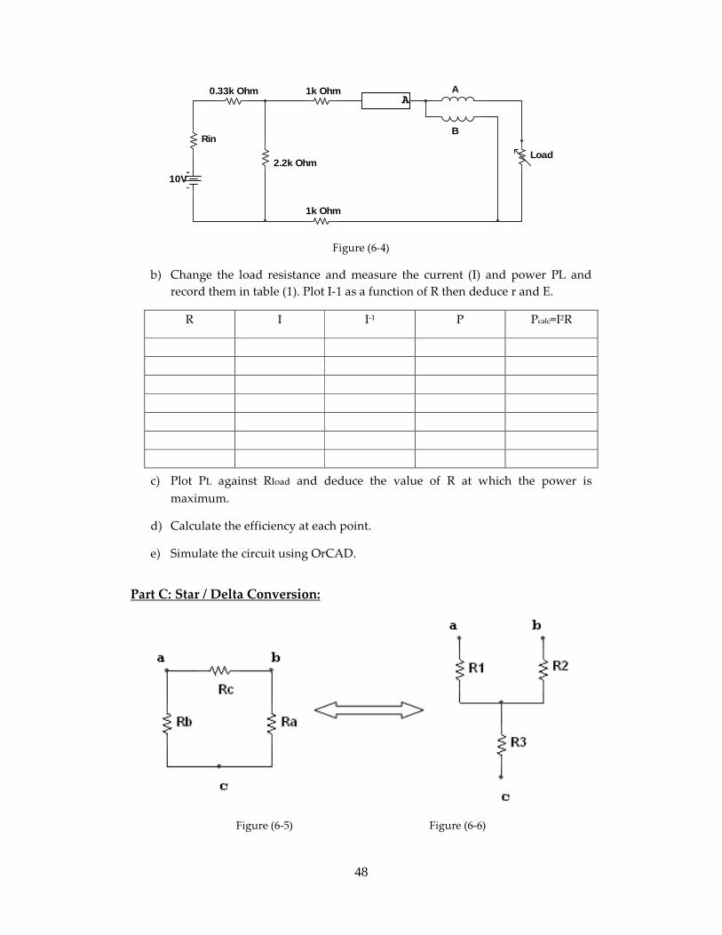
a) Connect the circuit as shown in figure (6-4).
48
10V
Rin
0.33k Ohm 1k Ohm
1k Ohm
2.2k OhmLoad
A
B
A
Figure (6-4)
b) Change the load resistance and measure the current (I) and power PL and
record them in table (1). Plot I-1 as a function of R then deduce r and E.
R I I-1 P Pcalc=I2R
c) Plot PL against Rload and deduce the value of R at which the power is
maximum.
d) Calculate the efficiency at each point.
e) Simulate the circuit using OrCAD.
Part C: Star / Delta Conversion:
Figure (6-5) Figure (6-6)
49
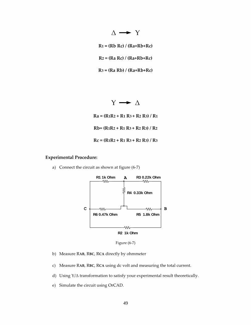
Δ Y
R1 = (Rb Rc) / (Ra+Rb+Rc)
R2 = (Ra Rc) / (Ra+Rb+Rc)
R3 = (Ra Rb) / (Ra+Rb+Rc)
Y Δ
Ra = (R1R2 + R1 R3 + R2 R3) / R1
Rb= (R1R2 + R1 R3 + R2 R3) / R2
Rc = (R1R2 + R1 R3 + R2 R3) / R3
Experimental Procedure:
a) Connect the circuit as shown at figure (6-7)
R1 1k Ohm R3 0.22k Ohm
R5 1.8k Ohm
R2 1k Ohm
R4 0.33k Ohm
R6 0.47k Ohm
A
BC
Figure (6-7)
b) Measure RAB, RBC, RCA directly by ohmmeter
c) Measure RAB, RBC, RCA using dc volt and measuring the total current.
d) Using Y/Δ transformation to satisfy your experimental result theoretically.
e) Simulate the circuit using OrCAD.
50
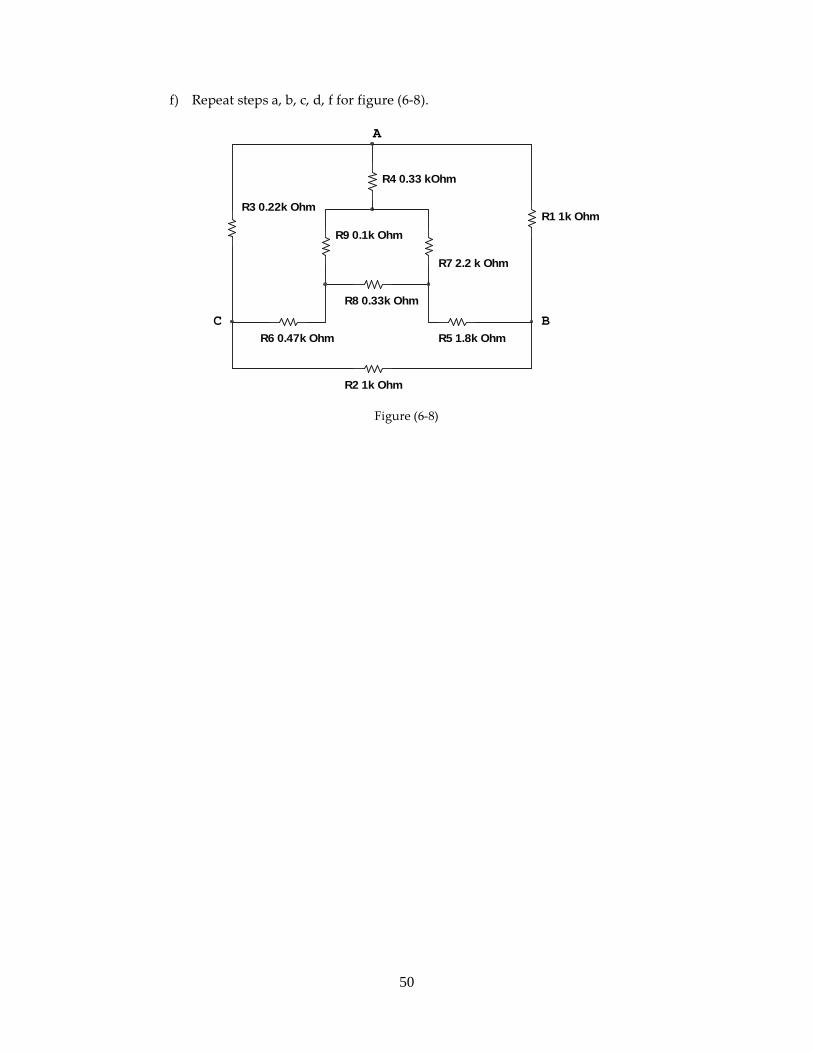
f) Repeat steps a, b, c, d, f for figure (6-8).
R2 1k Ohm
R5 1.8k OhmR6 0.47k Ohm
R8 0.33k Ohm
R9 0.1k Ohm
R7 2.2 k Ohm
R1 1k OhmR3 0.22k Ohm
R4 0.33 kOhm
C B
A
Figure (6-8)
51
ـــــــــــــــــــــــــــــــــــــــــــــــــــــــــــــــــــــــــــــــــــــــExperiment 7
RMS value of an AC Waveform ـــــــــــــــــــــــــــــــــــــــــــــــــــــــــــــــــــــــــــــــــــــــ
Objective :
- To know the concept of rms value.
- To measure rms values for different waveforms.
- To calculate the other important relations such as: form factor and peak
factor.
Theory:
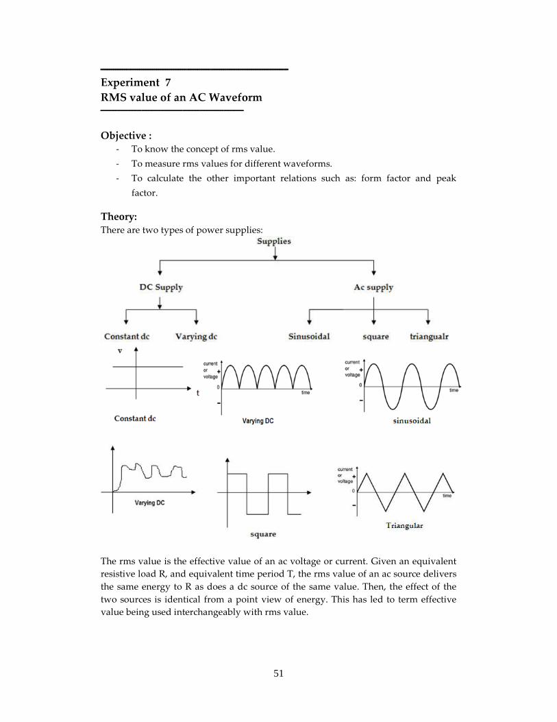
There are two types of power supplies:
The rms value is the effective value of an ac voltage or current. Given an equivalent
resistive load R, and equivalent time period T, the rms value of an ac source delivers
the same energy to R as does a dc source of the same value. Then, the effect of the
two sources is identical from a point view of energy. This has led to term effective
value being used interchangeably with rms value.
52
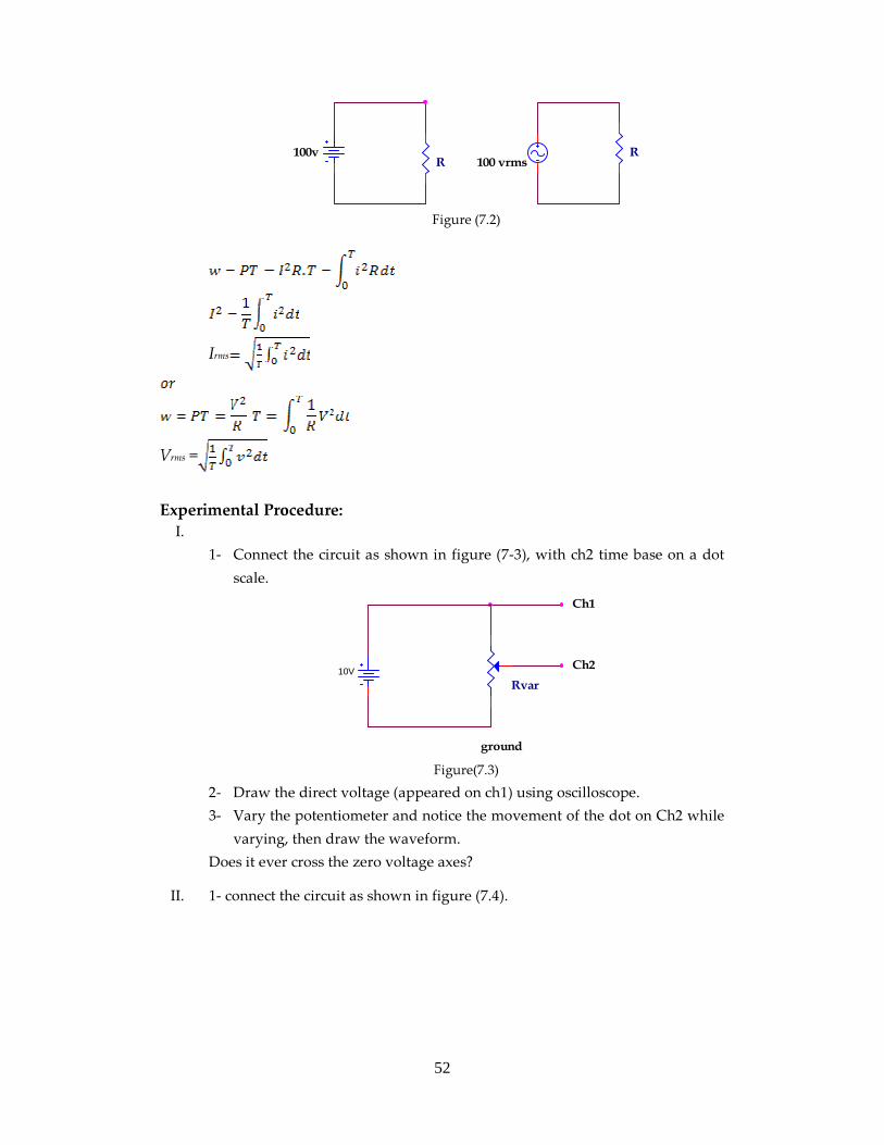
100vR
R100 vrms
Figure (7.2)
Irms
Vrms =
Experimental Procedure:
I.
1- Connect the circuit as shown in figure (7-3), with ch2 time base on a dot
scale.
Rvar10V
Ch1
Ch2
ground Figure(7.3)
2- Draw the direct voltage (appeared on ch1) using oscilloscope.
3- Vary the potentiometer and notice the movement of the dot on Ch2 while
varying, then draw the waveform.
Does it ever cross the zero voltage axes?
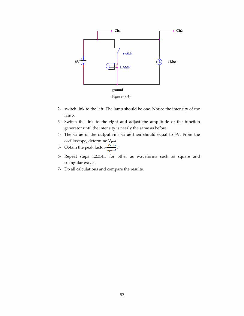
II. 1- connect the circuit as shown in figure (7.4).
53
5V
switch
1Khz
LAMP12
ground
Ch1 Ch2
Figure (7.4)
2- switch link to the left. The lamp should be one. Notice the intensity of the
lamp.
3- Switch the link to the right and adjust the amplitude of the function
generator until the intensity is nearly the same as before.
4- The value of the output rms value then should equal to 5V. From the
oscilloscope, determine Vpeak.
5- Obtain the peak factor= .
6- Repeat steps 1,2,3,4,5 for other as waveforms such as square and
triangular waves.
7- Do all calculations and compare the results.
54
ــــــــــــــــــــــــــــــــــــــــــــــــــــــــــــــــــــــــــــــــــــــــExperiment 8
Capacitors in Series and parallel ــــــــــــــــــــــــــــــــــــــــــــــــــــــــــــــــــــــــــــــــــــــــ
Objectives:
• To explore the idea of the capacitance of a component.
• To measure the value of the capacitance using DC supply.
• To investigate what happens when capacitors are connected in series and in
parallel.
Theoretical Background:
The capacitor consists of two metal plates, separated by an insulating layer. The
insulator may be air, or any other insulating material with suitable characteristics.
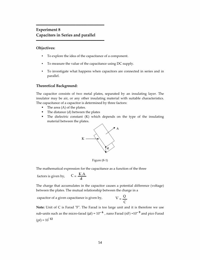
The capacitance of a capacitor is determined by three factors:
The area (A) of the plates.
The distance (d) between the plates
The dielectric constant (K) which depends on the type of the insulating
material between the plates.
Figure (8-1)
The mathematical expression for the capacitance as a function of the three
factors is given by,
The charge that accumulates in the capacitor causes a potential difference (voltage)
between the plates. The mutual relationship between the charge in a
capacitor of a given capacitance is given by,
Note: Unit of C is Farad "F". The Farad is too large unit and it is therefore we use
sub-units such as the micro-farad (µf) = 10– 6 , nano Farad (nF) =10– 9 and pico Farad
(pf) = 10 12 ـ
55
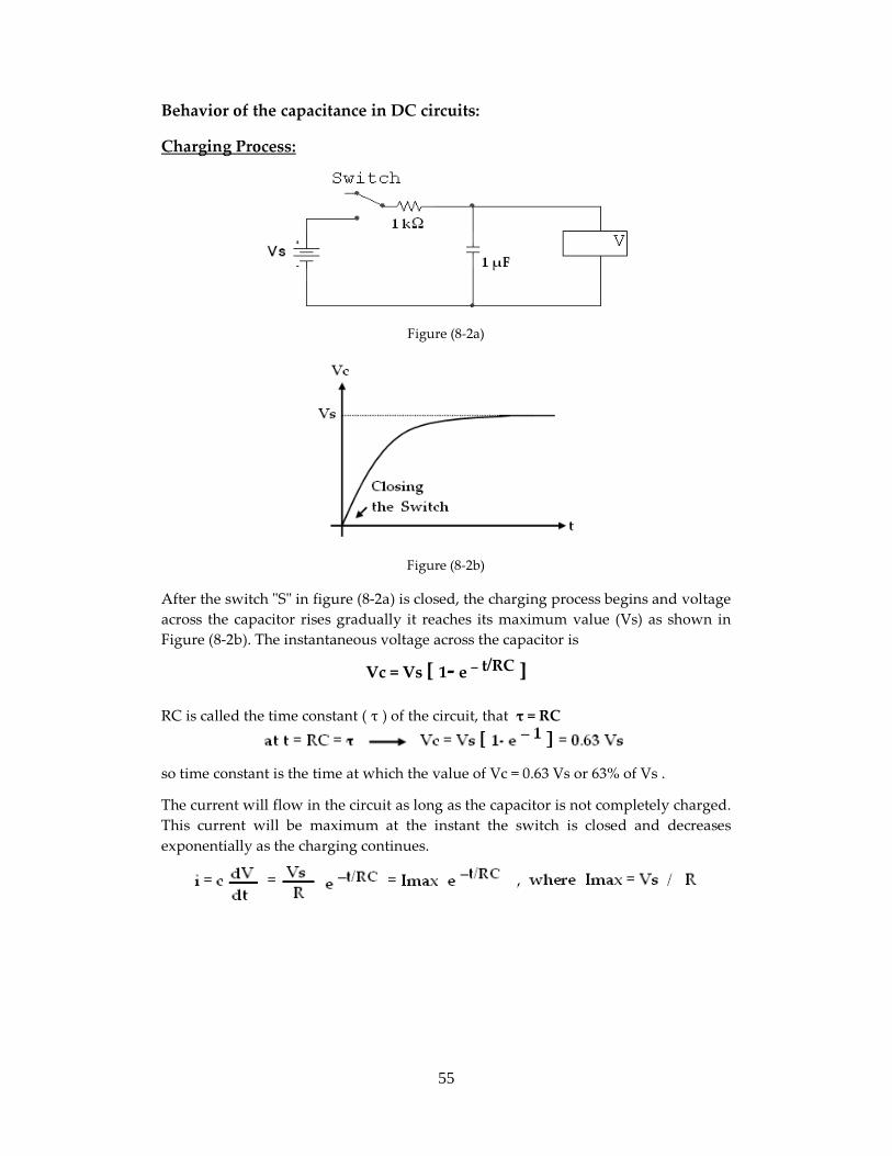
Behavior of the capacitance in DC circuits:
Charging Process:
Figure (8-2a)
Figure (8-2b)
After the switch "S" in figure (8-2a) is closed, the charging process begins and voltage
across the capacitor rises gradually it reaches its maximum value (Vs) as shown in
Figure (8-2b). The instantaneous voltage across the capacitor is
Vc = Vs [ 1- e – t/RC ] RC is called the time constant ( τ ) of the circuit, that τ = RC
so time constant is the time at which the value of Vc = 0.63 Vs or 63% of Vs .
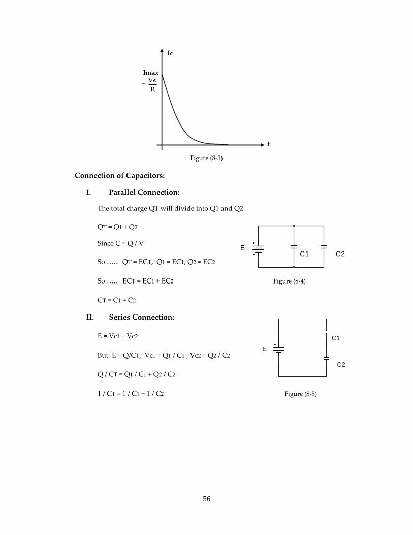
The current will flow in the circuit as long as the capacitor is not completely charged.
This current will be maximum at the instant the switch is closed and decreases
exponentially as the charging continues.
56
C1 C2E
C1
C2
E
Figure (8-3)
Connection of Capacitors:
I. Parallel Connection:
The total charge QT will divide into Q1 and Q2
QT = Q1 + Q2
Since C = Q / V
So ….. QT = ECT, Q1 = EC1, Q2 = EC2
So ….. ECT = EC1 + EC2 Figure (8-4)
CT = C1 + C2
II. Series Connection:
E = Vc1 + Vc2
But E = Q/CT, Vc1 = Q1 / C1 , Vc2 = Q2 / C2
Q / CT = Q1 / C1 + Q2 / C2
1 / CT = 1 / C1 + 1 / C2 Figure (8-5)
57
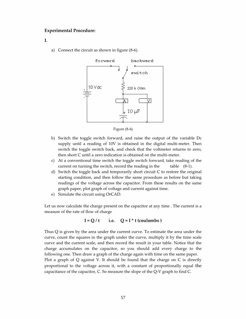
Experimental Procedure:
I.
a) Connect the circuit as shown in figure (8-6).
Figure (8-6)
b) Switch the toggle switch forward, and raise the output of the variable Dc
supply until a reading of 10V is obtained in the digital multi-meter. Then
switch the toggle switch back, and check that the voltmeter returns to zero,
then short C until a zero indication is obtained on the multi-meter. c) At a conventional time switch the toggle switch forward, take reading of the
current on turning the switch, record the reading in the table (8-1).
d) Switch the toggle back and temporarily short circuit C to restore the original
starting condition, and then follow the same procedure as before but taking
readings of the voltage across the capacitor. From these results on the same
graph paper, plot graph of voltage and current against time.
e) Simulate the circuit using OrCAD.
Let us now calculate the charge present on the capacitor at any time . The current is a
measure of the rate of flow of charge
I = Q / t i.e. Q = I * t (coulombs ) Thus Q is given by the area under the current curve. To estimate the area under the
curve, count the squares in the graph under the curve, multiply it by the time scale
curve and the current scale, and then record the result in your table. Notice that the
charge accumulates on the capacitor, so you should add every charge to the
following one. Then draw a graph of the charge again with time on the same paper.
Plot a graph of Q against V. It should be found that the charge on C is directly
proportional to the voltage across it, with a constant of proportionally equal the
capacitance of the capacitor, C. So measure the slope of the Q-V graph to find C.
58
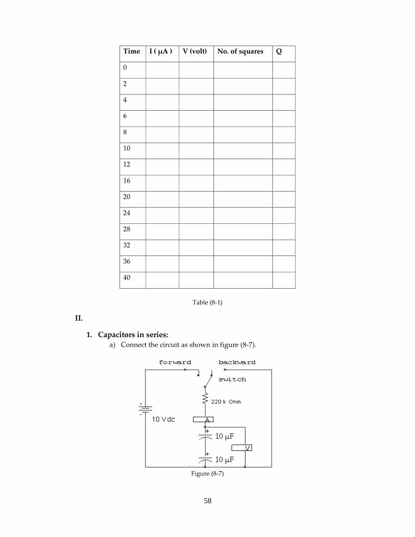
Time I ( µA ) V (volt) No. of squares Q
0
2
4
6
8
10
12
16
20
24
28
32
36
40
Table (8-1)
II.
1. Capacitors in series:
a) Connect the circuit as shown in figure (8-7).
Figure (8-7)
59
b) Repeat previous steps, plot a graph of current against time, and count
squares under the graph, and calculate the charge.
c) Plot a graph of Q against V and compute the slope to find CT, then
find a relation between C total, C1, and C2 for the series connection.
d) Simulate the circuit using Or-CAD.
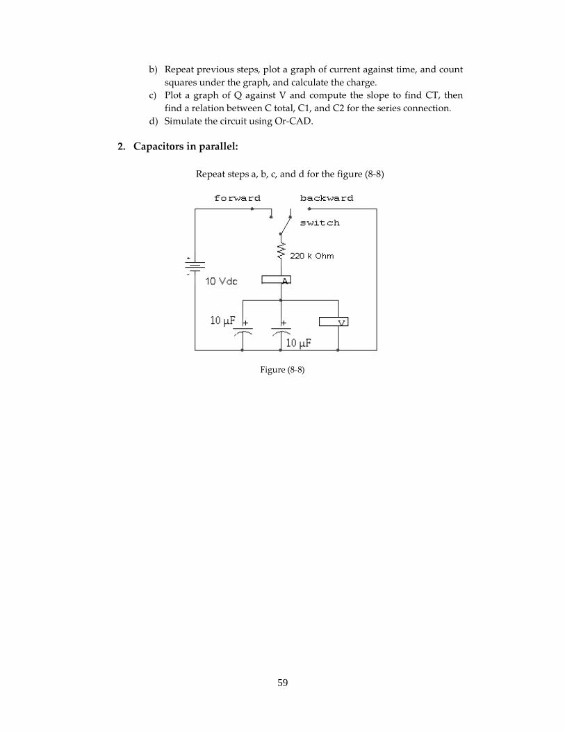
2. Capacitors in parallel:
Repeat steps a, b, c, and d for the figure (8-8)
Figure (8-8)
60
ــــــــــــــــــــــــــــــــــــــــــــــــــــــــــــــــــــــــــــــــExperiment 9
Time constant and inductance ــــــــــــــــــــــــــــــــــــــــــــــــــــــــــــــــــــــــــــــــ
Objective :
• To investigate the factors determining the charge and discharge time for a
capacitive and inductive circuits.
• To explore the idea of the inductance of a component.
Theory:
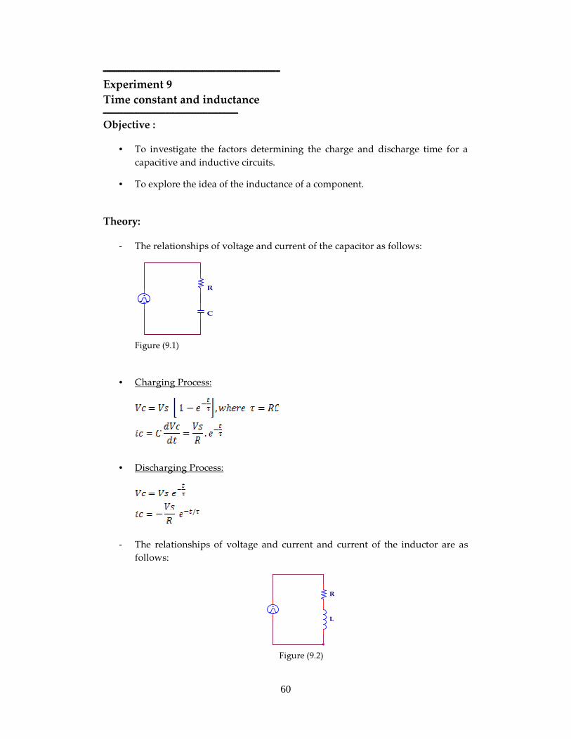
- The relationships of voltage and current of the capacitor as follows:
R
C
Figure (9.1)
• Charging Process:
• Discharging Process:
- The relationships of voltage and current and current of the inductor are as
follows:
R
L
Figure (9.2)

61
• Charging Process:
iL
• Discharging Process:
iL
Time
0s 0.5ms 1.0ms 1.5ms 2.0msV(L1:2)
-5.0V
0V
5.0V
Experimental Procedure:
I. 1- connect the circuit as shown in figure (9.5).
Time
0s 0.5ms 1.0ms 1.5ms 2.0ms-I(L1)
-5.0mA
0A
5.0mA Time
0s 0.5ms 1.0ms 1.5ms 2.0msV(C1:2)
-5.0V
0V
5.0V
Time
0s 0.5ms 1.0ms 1.5ms 2.0msV(L1:2,R1:2)
-10V
0V
10V
Time
0s 0.5ms 1.0ms 1.5ms 2.0ms-I(C2)
-10mA
0A
10mA
Time
0s 0.5ms 1.0ms 1.5ms 2.0msV(C2:2,R1:2)
-5.0V
0V
5.0V
Figure (9.3) Figure (9.4)
62
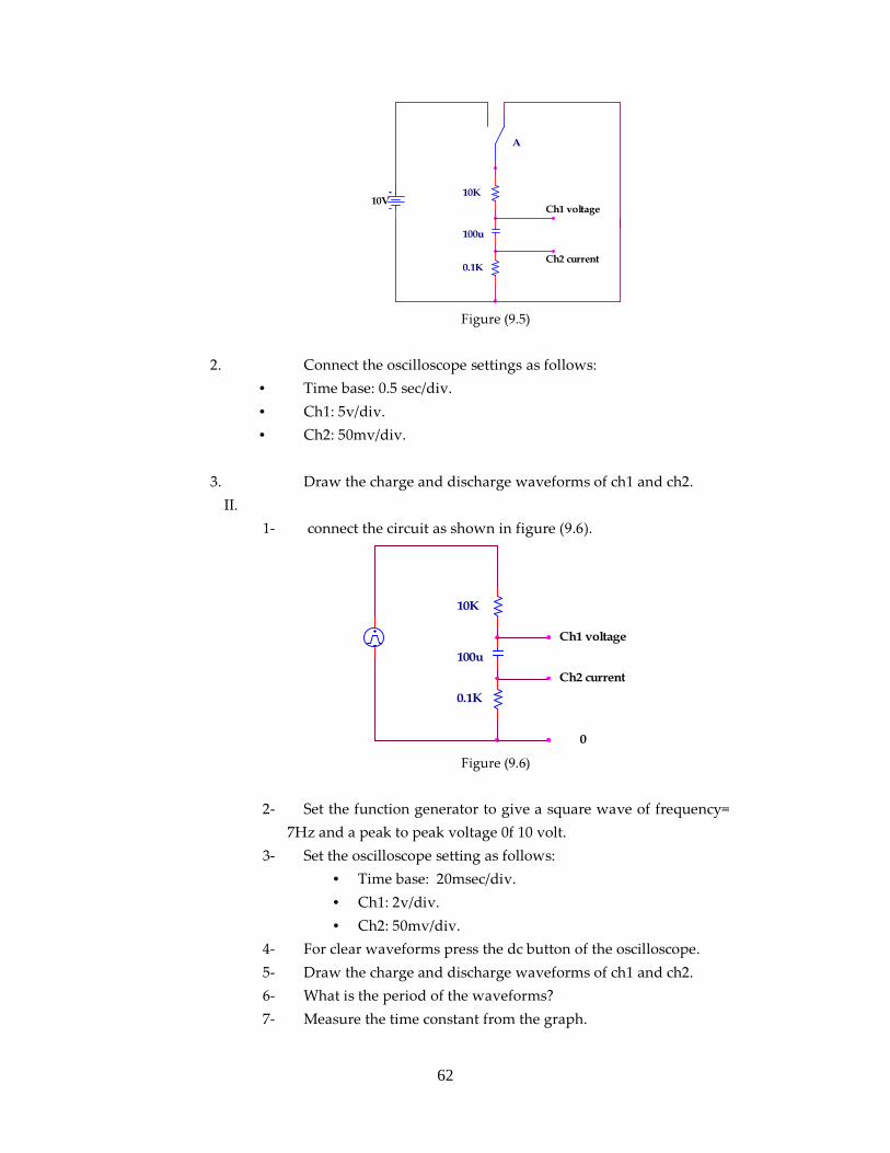
10V
A
10K
100u
0.1K
Ch1 voltage
Ch2 current
Figure (9.5)
2. Connect the oscilloscope settings as follows:
• Time base: 0.5 sec/div.
• Ch1: 5v/div.
• Ch2: 50mv/div.
3. Draw the charge and discharge waveforms of ch1 and ch2.
II.
1- connect the circuit as shown in figure (9.6).
10K
100u
0.1K
Ch1 voltage
Ch2 current
0 Figure (9.6)
2- Set the function generator to give a square wave of frequency=
7Hz and a peak to peak voltage 0f 10 volt.
3- Set the oscilloscope setting as follows:
• Time base: 20msec/div.
• Ch1: 2v/div.
• Ch2: 50mv/div.
4- For clear waveforms press the dc button of the oscilloscope.
5- Draw the charge and discharge waveforms of ch1 and ch2.
6- What is the period of the waveforms?
7- Measure the time constant from the graph.
63
8- Calculate the time constant theoretically, and then compare the
results.
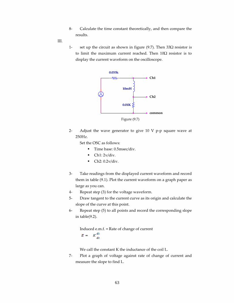
III.
1- set up the circuit as shown in figure (9.7). Then 33Ω resistor is
to limit the maximum current reached. Then 10Ω resistor is to
display the current waveform on the oscilloscope.
0.033k
10mH
0.01K
common
Ch1
Ch2
Figure (9.7)
2- Adjust the wave generator to give 10 V p-p square wave at
250Hz.
Set the OSC as follows:
Time base: 0.5msec/div.
Ch1: 2v/div.
Ch2: 0.2v/div.
3- Take readings from the displayed current waveform and record
them in table (9.1). Plot the current waveform on a graph paper as
large as you can.
4- Repeat step (3) for the voltage waveform.
5- Draw tangent to the current curve as its origin and calculate the
slope of the curve at this point.
6- Repeat step (5) to all points and record the corresponding slope
in table(9.2).
Induced e.m.f. = Rate of change of current
We call the constant K the inductance of the coil L.
7- Plot a graph of voltage against rate of change of current and
measure the slope to find L.
64
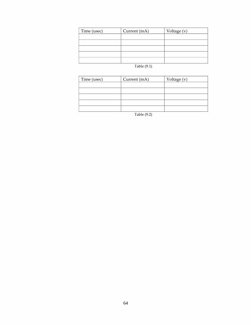
Time (usec) Current (mA) Voltage (v)
Table (9.1)
Time (usec) Current (mA) Voltage (v)
Table (9.2)
65
ـــــــــــــــــــــــــــــــــــــــــــــــــــــــــــــــــــــــــــــــــــــــــــــــــــــــــــــــــــــــــــــــــــــــــــــــ Experiment 10
A: Pulse Response of RL and RC
B: Resistive, Inductive, and capacitive at AC circuits ـــــــــــــــــــــــــــــــــــــــــــــــــــــــــــــــــــــــــــــــــــــــــــــــــــــــــــــــــــــــــــــــــــــــــــــــ
Part A: Pulse Response of RL and RC
Objective :
• To investigate the factors determining the time constant for RC, RL circuits.
• To investigate the pulse response of RL, RC circuits.
Theoretical Background :
The complete response of pulse signal flowing in RL, RC, circuit is composed of the
natural and forced response for the circuit at the same time.
There are three factors that affected the pulse response waveform:
1. Components of the circuit:
τ= RC in RC circuits
τ= L/R in RL circuits
For example : reducing R in RC circuit will reduce τ so the response will reach
the steady state value in faster time, and increasing R will make the response to
have a ramp form
2. Time period = 1/ f
The variation of frequency also affects the waveform of the pulse response.
For example : reducing frequency will expand the waveform and vice-versa.
3. Type of the input signal will affect the pulse response. It may be sine wave,
square wave, triangular wave … etc.
Experimental procedure:
I. Pulse response as a function of frequency:
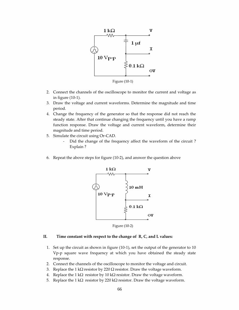
1. Set up the circuit as shown in figure (10-1). Set the output of the generator to 10
Vp-p square wave with the suitable frequency for the steady state response.
66
Figure (10-1)
2. Connect the channels of the oscilloscope to monitor the current and voltage as
in figure (10-1).
3. Draw the voltage and current waveforms. Determine the magnitude and time
period.
4. Change the frequency of the generator so that the response did not reach the
steady state. After that continue changing the frequency until you have a ramp
function response. Draw the voltage and current waveform, determine their
magnitude and time period.
5. Simulate the circuit using Or-CAD.
- Did the change of the frequency affect the waveform of the circuit ?
Explain ?
6. Repeat the above steps for figure (10-2), and answer the question above
Figure (10-2)
II. Time constant with respect to the change of R, C, and L values:
1. Set up the circuit as shown in figure (10-1), set the output of the generator to 10
Vp-p square wave frequency at which you have obtained the steady state
response.
2. Connect the channels of the oscilloscope to monitor the voltage and circuit.
3. Replace the 1 kΩ resistor by 220 Ω resistor. Draw the voltage waveform.
4. Replace the 1 kΩ resistor by 10 kΩ resistor. Draw the voltage waveform.
5. Replace the 1 kΩ resistor by 220 kΩ resistor. Draw the voltage waveform.
67
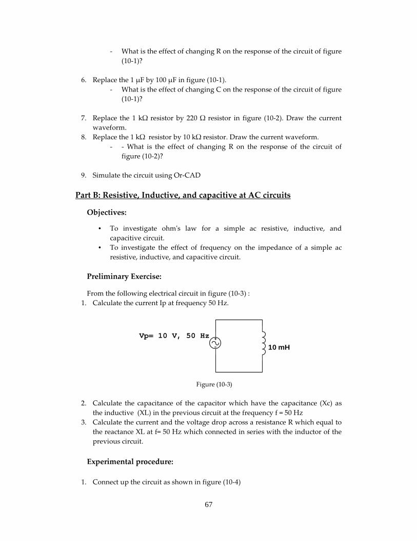
- What is the effect of changing R on the response of the circuit of figure
(10-1)?
6. Replace the 1 µF by 100 µF in figure (10-1).
- What is the effect of changing C on the response of the circuit of figure
(10-1)?
7. Replace the 1 kΩ resistor by 220 Ω resistor in figure (10-2). Draw the current
waveform.
8. Replace the 1 kΩ resistor by 10 kΩ resistor. Draw the current waveform.
- - What is the effect of changing R on the response of the circuit of
figure (10-2)?
9. Simulate the circuit using Or-CAD
Part B: Resistive, Inductive, and capacitive at AC circuits
Objectives:
• To investigate ohm's law for a simple ac resistive, inductive, and
capacitive circuit.
• To investigate the effect of frequency on the impedance of a simple ac
resistive, inductive, and capacitive circuit.
Preliminary Exercise:
From the following electrical circuit in figure (10-3) :
1. Calculate the current Ip at frequency 50 Hz.
10 mH
Vp= 10 V, 50 Hz
Figure (10-3)
2. Calculate the capacitance of the capacitor which have the capacitance (Xc) as
the inductive (XL) in the previous circuit at the frequency f = 50 Hz
3. Calculate the current and the voltage drop across a resistance R which equal to
the reactance XL at f= 50 Hz which connected in series with the inductor of the
previous circuit.
Experimental procedure:
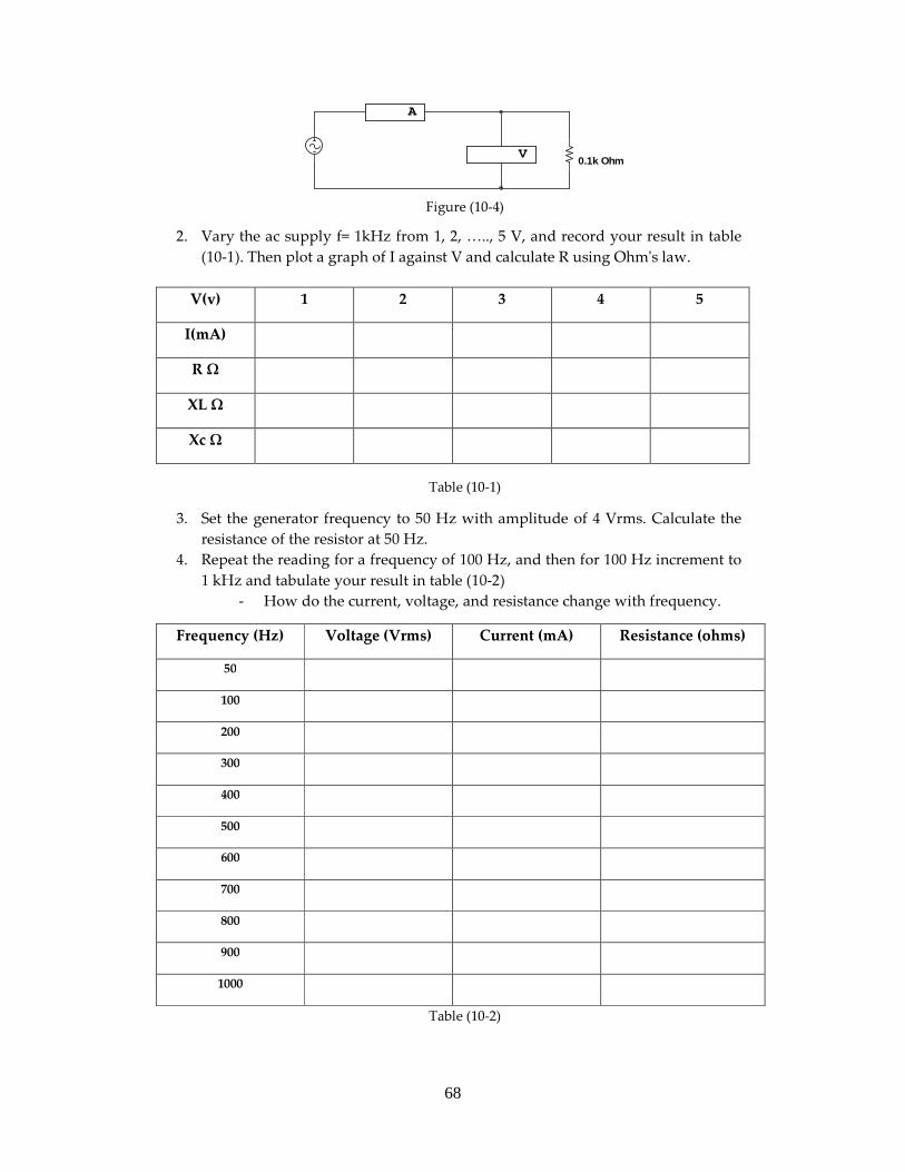
1. Connect up the circuit as shown in figure (10-4)
68
0.1k Ohm
A
V
Figure (10-4)
2. Vary the ac supply f= 1kHz from 1, 2, ….., 5 V, and record your result in table
(10-1). Then plot a graph of I against V and calculate R using Ohm's law.
V(v) 1 2 3 4 5
I(mA)
R Ω
XL Ω
Xc Ω
Table (10-1)
3. Set the generator frequency to 50 Hz with amplitude of 4 Vrms. Calculate the
resistance of the resistor at 50 Hz.
4. Repeat the reading for a frequency of 100 Hz, and then for 100 Hz increment to
1 kHz and tabulate your result in table (10-2)
- How do the current, voltage, and resistance change with frequency.
Frequency (Hz) Voltage (Vrms) Current (mA) Resistance (ohms)
50
100
200
300
400
500
600
700
800
900
1000
Table (10-2)
69
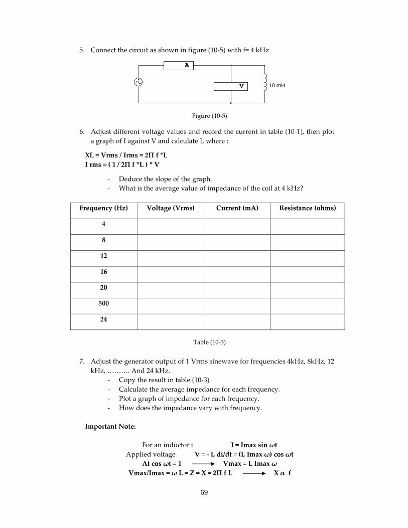
5. Connect the circuit as shown in figure (10-5) with f= 4 kHz
10 mH
A
V
Figure (10-5)
6. Adjust different voltage values and record the current in table (10-1), then plot
a graph of I against V and calculate L where :
XL = Vrms / Irms = 2Π f *L
I rms = ( 1 / 2Π f *L ) * V
- Deduce the slope of the graph.
- What is the average value of impedance of the coil at 4 kHz?
Frequency (Hz) Voltage (Vrms) Current (mA) Resistance (ohms)
4
8
12
16
20
500
24
Table (10-3)
7. Adjust the generator output of 1 Vrms sinewave for frequencies 4kHz, 8kHz, 12
kHz, ………. And 24 kHz.
- Copy the result in table (10-3)
- Calculate the average impedance for each frequency.
- Plot a graph of impedance for each frequency.
- How does the impedance vary with frequency.
Important Note:
For an inductor : I = Imax sin ωt
Applied voltage V = - L di/dt = (L Imax ω) cos ωt
At cos ωt = 1 Vmax = L Imax ω
Vmax/Imax = ω L = Z = X = 2Π f L X α f
70
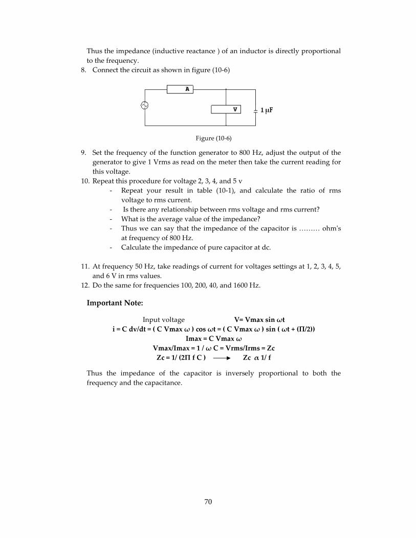
Thus the impedance (inductive reactance ) of an inductor is directly proportional
to the frequency.
8. Connect the circuit as shown in figure (10-6)
Figure (10-6)
9. Set the frequency of the function generator to 800 Hz, adjust the output of the
generator to give 1 Vrms as read on the meter then take the current reading for
this voltage.
10. Repeat this procedure for voltage 2, 3, 4, and 5 v
- Repeat your result in table (10-1), and calculate the ratio of rms
voltage to rms current.
- Is there any relationship between rms voltage and rms current?
- What is the average value of the impedance?
- Thus we can say that the impedance of the capacitor is ……… ohm's
at frequency of 800 Hz.
- Calculate the impedance of pure capacitor at dc.
11. At frequency 50 Hz, take readings of current for voltages settings at 1, 2, 3, 4, 5,
and 6 V in rms values.
12. Do the same for frequencies 100, 200, 40, and 1600 Hz.
Important Note:
Input voltage V= Vmax sin ωt
i = C dv/dt = ( C Vmax ω ) cos ωt = ( C Vmax ω ) sin ( ωt + (Π/2))
Imax = C Vmax ω
Vmax/Imax = 1 / ω C = Vrms/Irms = Zc
Zc = 1/ (2Π f C ) Zc α 1/ f
Thus the impedance of the capacitor is inversely proportional to both the
frequency and the capacitance.
71
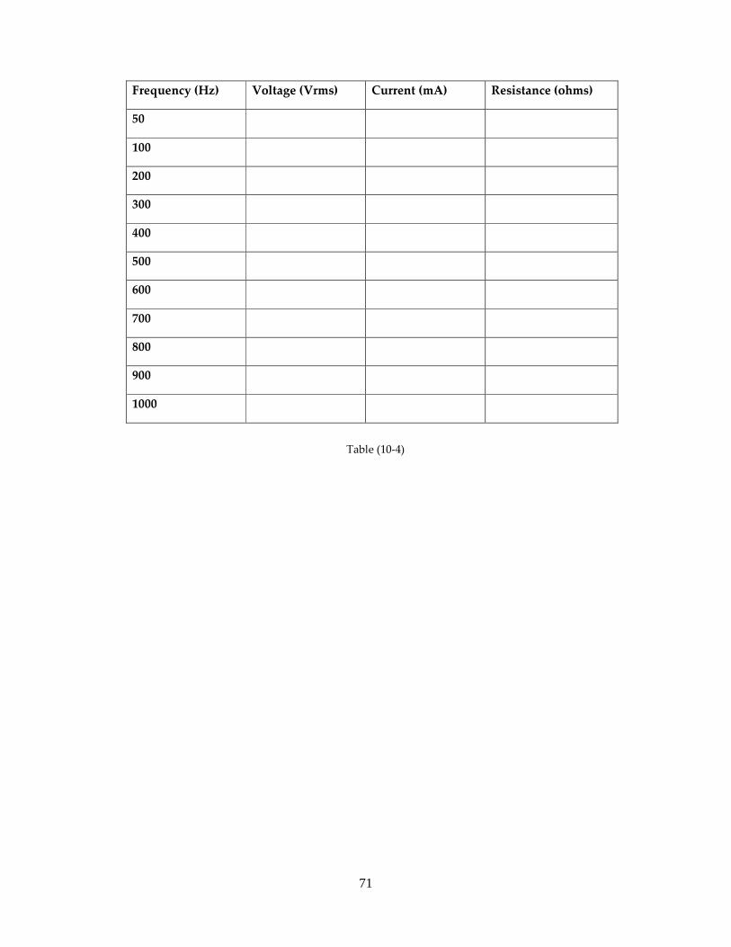
Frequency (Hz) Voltage (Vrms) Current (mA) Resistance (ohms)
50
100
200
300
400
500
600
700
800
900
1000
Table (10-4)
72
ــــــــــــــــــــــــــــــــــــــــــــــــــــــــــــــــــــــــ
Experiment 11
Damping in RLC circuits ـــــــــــــــــــــــــــــــــــــــــــــــــــــــــــــــــــــــ
Objective :
To investigate the over, under, and critical damping in series and parallel
RLC circuits .
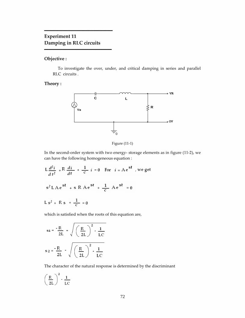
Theory :
0
C L
RVs
VR
OV
Figure (11-1)
In the second-order system with two energy- storage elements as in figure (11-2), we
can have the following homogeneous equation :
which is satisfied when the roots of this equation are,
The character of the natural response is determined by the discriminant
73
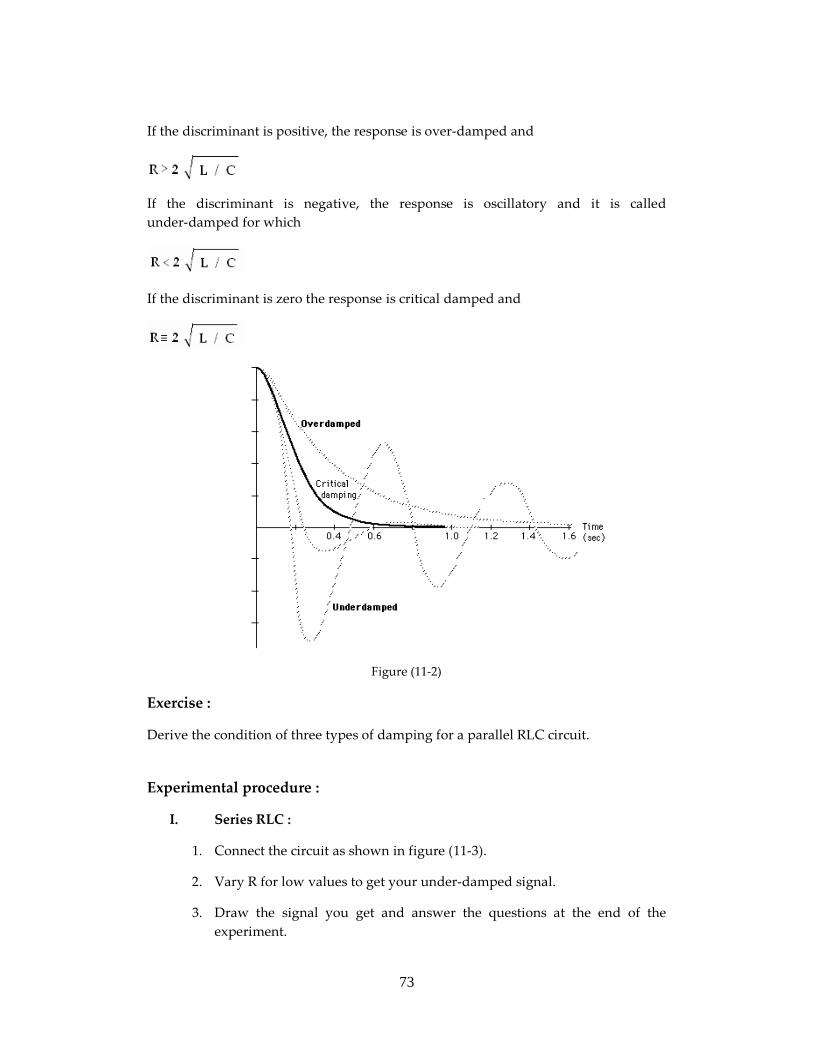
If the discriminant is positive, the response is over-damped and
If the discriminant is negative, the response is oscillatory and it is called
under-damped for which
If the discriminant is zero the response is critical damped and
Figure (11-2)
Exercise :
Derive the condition of three types of damping for a parallel RLC circuit.
Experimental procedure :
I. Series RLC :
1. Connect the circuit as shown in figure (11-3).
2. Vary R for low values to get your under-damped signal.
3. Draw the signal you get and answer the questions at the end of the
experiment.

74
4. Change the frequency and explain what happens.
5. Now vary the resistor for mid values to get your critical damping signal
and repeat steps 3 and 4.
6. Vary R for high values to get your over-damping signal, and then repeat
steps 3,4.
0
2.2 u F
R
10 mH
3 Vpp, 50 Hz
VR
OV
Figure (11-3)
II. Parallel RLC :
1. Connect the circuit as shown in figure (11-4).
0
2.2 u F R10 mH
3 Vpp, 50 Hz
VR
OV
Figure (11-4)
2. Vary R to get your under-damping signal and repeat steps 3 and 4 from
part I.
3. Now vary R to get your critical damping signal. Repeat steps 3,4.
4. Vary R to get your over-damping signal. Repeat steps 3,4 above.
Discussion:
1. Find the time period for the oscillating signal and the range of resistor
variation.
2. Find the maximum peak value for the signal.

75
3. What happens when you increase or decrease R ?
4. Calculate the resonance frequency, damping coefficient and damping factor.
5. By calculation, draw V(t) for over-damping parallel circuit, and under
damping series RLC circuit.