Embed Size (px)
Citation preview

Eindhoven University of Technology
MASTER
Self-sensing magnetic levitation : a feasibility study
van Acht, V.M.G.
Award date:1997
DisclaimerThis document contains a student thesis (bachelor's or master's), as authored by a student at Eindhoven University of Technology. Studenttheses are made available in the TU/e repository upon obtaining the required degree. The grade received is not published on the documentas presented in the repository. The required complexity or quality of research of student theses may vary by program, and the requiredminimum study period may vary in duration.
General rightsCopyright and moral rights for the publications made accessible in the public portal are retained by the authors and/or other copyright ownersand it is a condition of accessing publications that users recognise and abide by the legal requirements associated with these rights.
• Users may download and print one copy of any publication from the public portal for the purpose of private study or research. • You may not further distribute the material or use it for any profit-making activity or commercial gain
Take down policyIf you believe that this document breaches copyright please contact us providing details, and we will remove access to the work immediatelyand investigate your claim.
Download date: 23. Jul. 2018

University of Technology EindhovenDepartment of Electrical EngineeringMeasurement and Control Section
Self-SensingMagnetic LevitationA Feasibility Study
by V.M.G. van Acht
09-06-9722:08:00,25, UKMaster of Science ThesisCarried out from October 1996 to June 1997Commissioned by prof.drjr. P.PJ. van den BoschUnder supervision of dr.ir. A. Darnen

Eindhoven University of Technology
IABSTRACT
Department of Electrical Engineering Measurement and Control Group
At the Eindhoven University of Technology research is carried out at a three dimensionallaser interferometer, which can be used to measure the position of an object. (For example thetool centre point of a robot.) In the laser-interferometer a mirror is used to direct the laserbeam onto a retro-reflector on the object to be measured. The position and orientation of thismirror must be controlled extremely accurate and fast.One way to realise the laser deflection system is to use magnetic bearings. Magnetic bearingshave the advantage that friction is extremely low, tracking can be extremely accurate (inprinciple) and hardware is cheap. Magnetic bearings use several electromagnetic coils to exertpositioning forces onto the freely levitated ferromagnetic mirror. One way to obtain theposition and orientation of the mirror (necessary for the position control system of the mirror)is to measure the inductances of the same coils which are used to levitate the mirror. This iscalled selfsensing magnetic levitation. Self sensing magnetic levitation has the advantage thatno additional position sensors are necessary. Therefore it can be cheaper and smaller.
In this master of science thesis a pilot project for the magnetic levitated mirror is discussed. Asteel ball is to be levitated and controlled in the two directions ofthe vertical plane by fourcoils. Position of the ball must be obtained by measuring the inductances of the coils.First the magnetic, electrical and mechanical parameters of the levitation system aremeasured. After that, the equations of a one-dimensional magnetic levitation system arederived for current controlled coils and voltage controlled coils. Then the two differentactuators (current source and voltage source) are examined in detail. It will be shown that, incontrary to a voltage source, a current source is very likely to oscillate and suffers from a lotof output voltage noise when loaded with a coil. Next, five different ways to measure theinductances of the coils are discussed and examined in detail, and the best actuator/sensorcombination is chosen. It will appear that this is a voltage controlled current source with anadditional HF-component to measure the inductance of the coil.After that, a controller is designed for the magnetic levitated ball, using the previously chosenactuator/sensor combination, and simulations with the proposed controller are done.Finally the designed actuator and sensor are tested in practice, and recommendations are givenregarding the magnetic levitated mirror system.
3
Eindhoven University of Technology
CONTENTS
Department of Electrical Engineering Measurement and Control Group
AbstractContentsList of FiguresList of TablesList of Used Symbols1. Introduction2. Model Parameters
2.1. Measuring Coil Saturation2.2 Measuring Small-Signal Coil Parameters2.3 Measuring Position / Inductance Relation
3. Theory of Magnetic Levitation3.1 Derivation of the Coil Equations
3.1.1 Current Control3.1.2 Voltage Control
3.2 Conclusions4. Actuators
4.1 Linear Current Source4.1.1 Problems with the Current Source4.1.2 Hoo Controller Design, Current Sensing4.1.3 Hoo Controller Design, Current and Voltage Sensing4.1.4 Simulations of the Designed Current Sources4.1.5 Conclusions Regarding Current Sources
4.2 Linear Voltage Source4.3 Switched Power Supplies
4.3.1. Pulse Width Modulated Power Supply4.3.2 PWM / FM Power Supply4.3.3 PWM Power Supply with Additional High Frequency Component4.3.4 Serial Resonant Switched Power Supply4.3.5 Parallel Resonant Switched Power Supply
4.4 Conclusions Regarding the Actuator5. Sensors
5.1 Measuring LC-Oscillation Frequency With PLL5.1.1 LC-oscillator with Voltage Source5.1.2 LC-oscillator with Current Source5.1.3 Measuring Frequency With a PLL
5.2 Measuring LC-Oscillation Frequency With HF-counter5.3 Measuring LC-Oscillator Q-factor5.4 Measuring Additional High Frequency Component
5.4.1 High Frequency Component with Voltage Control5.4.2 High Frequency Component with Current Control
5.5 Correlation Measurement5.6 Conclusions Regarding the Sensor
6. Choosing Actuator / Sensor Combination6.1 Choosing Actuator/Sensor Combination
6.2 Sensor Tuning
34679
10131416161818222325262626273339474749495151535557585960626467697070747778797980
4

Eindhoven University of Technology Department of Electrical Engineering Measurement and Control Group
7. Controller Design7.1 Second Order Linear Controller7.2 Third Order Linear Controller7.3 Third Order Non Linear Controller
7.4 Reo -controller7.5 Simulations7.6 Conclusions
8. Practical Implementation8.1 Testing Actuator8.2 Testing Inductance Sensor
9. Reflecting Achieved Goals to Mirror Deflection SystemLiteratureAppendix A. Measurement of Saturation of Magnetic MaterialsAppendix B. Measurement of Position / Inductance Relation
82838485
889498999999
101105107110
5
Eindhoven University of Technology Department of Electrical Engineering Measurement and Control Group
LIST OF FIGURES
figure 1: 3D laser interferometer 10figure 2: Magnetic levitated mirror 11figure 3: Magnetic bearing, pilot project 11figure 4: Physical dimensions of the process 13figure 5: Plot of saturation of coil material 14figure 6: Magnetic properties of materials 15figure 7: Position / inductance relation 17figure 8: One dimensional levitation system 19figure 9: Vertical least mean square fits on coil measurements 20figure 10: Flux lines through coil and ball 20figure 11: Voltage Controlled Current Source 27figure 12: Equivalent circuit of a current source loaded with a coil 27figure 13: Augmented plant 28figure 14: Generalised plant for MHC-Toolbox 28figure 15: Weighting filters for MHC-Toolbox 31figure 16: Controller designed by MHC-Toolbox 32figure 17: Voltage Controlled Current Source with voltage sensing 33figure 18: Augmented plant VCCS with voltage sensing 34figure 19: Generalised plant for MHC-Toolbox VCCS with voltage sensing 34figure 20: Weighting filters for MHC-Toolbox, VCCS with voltage sensing 37figure 21: Controller designed by MHC-Toolbox, VCCS with voltage sensing 38figure 22: Circuit ofVCCS with P-controller 40figure 23: Circuit ofVCCS with Hoo controller, current sensing only 40figure 24: Circuit ofVCCS with Hoo controller, current and voltage sensing 40figure 25: Output voltage VCCS with P-controller 41figure 26: Output voltage VCCS with Hoo controller, current sensing only 42figure 27: Tracking VCCS with Hoo controller, current sensing only 42figure 28: Phase shift of output current Hoo controller, current sensing only 43figure 29: Sensor noise to output current ofHoo controller, current sensing only 43figure 30: System noise to output voltage ofHoo controller, current sensing only 44figure 31: Output voltage of VCCS with Hoo controller, current and voltage sensing 44figure 32: Tracking VCCS with Hoo controller, current and voltage sensing 45figure 33: Phase output current Hoo controller, current and voltage sensing 45figure 34: Current sensor noise to output current Hoo controller, current and voltage sensing 46figure 35: Voltage sensor noise output current Hoo controller, current and voltage sensing 46figure 36: System noise amplification output voltage Hoo controller, current and voltage
sensing 47figure 37: Voltage Controlled Voltage Source 48figure 38: Circuit ofPWM supply 49figure 39: Equivalent circuits for PWM power supply 50figure 40: Saw-tooth component on I . 51figure 41: Voltage over the coil in PWM supply with additional high frequency component 52figure 42: Current through the coil in PWM supply with additional high frequency component52figure 43: Circuit of serial resonant switched power supply 54figure 44: Circuit of parallel resonant switched power supply 55
6

Eindhoven University ofTechnology Department of Electrical Engineering Measurement and Control Group
figure 45: Signals in parallel resonant switched power supply 56figure 46: LC-Oscillator sensor 59figure 47: LC-Oscillator sensor, with LC-filter 60figure 48: Equivalent scheme for calculating influence ofRL 60figure 49: Equivalent scheme for calculating influence ofRf 61figure 50: Equivalent scheme for calculating influence of Lf and Cf 62figure 51: LC-oscillator with current source 63figure 52: Phase Locked Loop 64figure 53: Ratio between BL and B3dB 66figure 54: Input signal of the hysterese-comparator 67figure 55: Enlargement of noisy signal around Vhys 67figure 56: Equivalent schematic for Q-factor measurement 70figure 57: Phase diagram of current and voltage over coil 71figure 58: Current sensing resistor circuitry 72figure 59: Phase diagram of current and voltage over coil 74figure 60: Time I influence I noise exchange 80figure 61: Block scheme of magnetic levitation system 82figure 62: Pole and zero map of the open loop system 83figure 63: Rootloci of controlled system, K=-900, zl 2=-21±lOj 84,figure 64: Root loci of controlled system, K=-2775, zl=40,z2=z3=60 85figure 65: Root loci of the controlled linearised system, around the nominal operation point 86figure 66: Exact linearisation 87figure 67: Augmented plant 88figure 68: Generalised plant for MRC-Toolbox 88figure 69: Weighting filters for MRC-Toolbox 91figure 70: Controller designed by MRC-Toolbox 92figure 71: Rootloci of the Roo controlled system 93figure 72: Two-coil-control 94figure 73: Simulink block scheme of controlled levitation system 95figure 74: Simulink block scheme of non linear process 95figure 75: Simulink block scheme of non linear controller 95figure 76: Simulation of the third order non linear controller 96figure 77: Simulation of the Roo non linear controller 97figure 78: Simulation ofthe Roo non linear controller, frequencies above specs. 97figure 79: Simulations of the Roo controller, noisy position measurement 97figure 80: Circuitry ofVCCS source, with minor adjustments 99figure 81: Circuitry of inductance sensor 100figure 82: Degrees of freedom of magnetic levitated mirror 101figure 83: Magnetic levitated ball with capasitive sensor 103figure 84: Alternative capasitive sensor for magnetic levitated mirror 104
I LIST OF TABLES
table 1: Physical dimensions of the processtable 2: Small signal coil parameterstable 3:Functions to combine two frequencies in switched power supplytable 4: Summarisation of actuators and sensors
13165279
7

Eindhoven University of Technology Department of Electrical Engineering Measurement and Control Group
LIST OF USED SYMBOLS
In this list only global symbols are given. They can be overrid by local definitions.
A = coil model parameter [H] [kg m2 s-2 A-2]
Ao = open loop amplification opamp []B = coil model parameter [m-I]
Cf = filter capacitance [F] [A2 s4 kg m-2]
J = frequency of additional high freq. [s-I]
Jo = resonance frequency [s-I]
Jg = gravitational force [N] [kg m s-2]
Jm = magnetic reluctance force [N] [kg m s-2]
Jose = oscillation frequency oscillator [s-I]g = gravitational acceleration [m s-2]iL = current through coil [A]L = inductance of the coil [H] [kg m2 s-2 A-2]Lf = filter inductance [H] [kg m2 s-2 A-2]
Ls = leak inductance [H] [kg m2 s-2 A-2]
m = mass of the levitated ball [kg]N = number of winding [1]Rf = filter resistance [0] [kg m2 s-3 A-2]
RL = resistance of the coil [0] [kg m2 s-3 A-2]
(SNR)in = signal to noise ratio, input signal [](SNR)out = signal to noise ratio, output signal []T = period of switched power supply [s]VL = coil voltage [V] [kg m2 s-3 A-I]Vdd = supply voltage [V] [kg m2 s-3 A-I]
VL = coil voltage [V] [kg m2 s-3 A-I]Vn = noise voltage [V] [kg m2 s-3 A-I]Vs = signal voltage [V] [kg m2 s-3 A-I]Vss = ground voltage or negative supply [V] [kg m2 s-3 A-I]
x = gap length [m]
8 = duty cycle of switched power supply [](/J = flux [Wb] [kg m2 s-2 A]
flo = permeability of vacuum [Him] [kg m s-2 A-2]
flr = relative permeability []r = time constant opamp [s]
9

Eindhoven University of Technology Department of Electrical Engineering Measurement and Control Group
11. INTRODUCTION
At the Eindhoven University of Technology, Measurement and Control Section, research isdone at a three dimensional laser interferometer, which can be used to measure to position ofan object (for example the tool centre point of a robot) very accurately in all three degrees offreedom. In figure 1 the 3D interferometer system is depicted.
retro reflector
laser deflection system
Dlase, I '"le""romete,
It tool centre point
~j half pass mirror \
'-1T'i'I:I:: I, I
I'!
cco
figure 1: 3D laser interferometer
In figure 1 a laser beam goes through a half pass mirror and is directed by the laser deflectionsystem onto the retro reflector on the tool centre point (TCP) ofthe robot. The retro reflectorreflects the laser beam back via the laser deflection system on the half pass mirror. Half of thelaser-beam is then reflected onto the CCD (charge coupled device), and the other half isreflected back into the laser interferometer. The interferometer is now able to measure thedistance the laser light has travelled.A control system controls the direction of the deflection mirror in such way that the laserbeam hits the CCD in the middle. The orientation of the mirror determines (in combinationwith the distance) the position of the tool centre point.
Biggest problem of the 3D laser interferometer as described above, is that the position and theorientation of the deflection mirror must be controlled extremely accurate and fast. (Goals arean accuracy of 1~.trad with a bandwidth of300 Hz) Therefore special bearings are necessary.At the Measurement and Control Section, an air bearing is used to control the position andangles of the mirror to deflect the laser beam. As this bearing has its limitations, the idea ofdeveloping a magnetic bearing was suggested. A magnetic bearing could be realised asshown in figure 2. Here the mirror is levitated and rotated by the same magnets. Probably thiswill lead to various problems, but figure 2 is only intended as an illustration of the magneticbearing for the laser deflection mirror.
10

Eindhoven University of Technology Department of Electrical Engineering Measurement and Control Group
figure 2: Magnetic levitated mirror
As a pilot project for the magnetic levitated mirror, to learn about magnetic bearings, amagnetic levitation system as in figure 3 has been developed.
figure 3: Magnetic bearing, pilotproject
The system as depicted in figure 3 consists of four electromagnets to position a steel ball intwo directions. The currents through the magnets are supplied by four power amplifiers,which are controlled by a controller.Special about this system is that it is selfsensing. This means that no explicit position sensoris used in the levitation system but that the position of the ball is obtained by measuring theinductances of the coils. Self sensing magnetic bearing are described in [1], [2], [3] and [5].The advantage of self sensing magnetic levitation is that it can be cheaper and smaller,evidently because of the absence of position sensors.
11

Eindhoven University of Technology Department of Electrical Engineering Measurement and Control Group
The pilot project, as described above, was already realised. However, there were a few majorproblems. First of all, the current through the coil was supplied by a current source. This hassome disadvantages, as will be made clear in chapter 4. The next problem was that theposition of the ball was not measured with the upper coil as it was levitated with, but with thebottom coil. Further on, the ball was not positioned in two dimensions but in the verticaldirection only. And last but not least, the controller was not able to stabilise the ball veryaccurately.Goal of this Master Science Thesis was to solve (some) of the problems of the self sensingmagnetic levitated ball.To write this Thesis the author has intensively used three other theses of the EindhovenUniversity of Technology, [10], [11] and [12]. Citations from these reports will be madewithout further notice.
12

Eindhoven University of Technology Department of Electrical Engineering Measurement and Control Group
112. MODEL PARAMETERS
Before any hardware or a controller can be designed the model parameters for the twodimensional magnetic levitation system must be obtained. This will be described in thischapter.The dimensions and some of the magnetic properties of the physical process are depicted infigure 4 and table 1.
-~ ~~
'"~~
~
'"~'"~
.G1}.r~
a
N
figure 4: Physical dimensions ofthe process
variable description value unita depth of coil 0.025 [m]b width of coil 0.025 [m]I length of coil 0.010 [m]
A(=a·b) area of coil 0.0625 [m2]
N number of turns 1000
Pc reI. permeability coil ~1000
(ferrox cube)c diameter ball 0.020 [m]m mass of ball 0.080 [kg]
Ph reI. permeability ball ~1000
(steel)
table 1: Physical dimensions ofthe process
Note that the upper coil has two separate windings, so there is a total of five coils. (not four)
13
Eindhoven University of Technology Department of Electrical Engineering Measurement and Control Group
k1. MEASURING COIL SATURATION
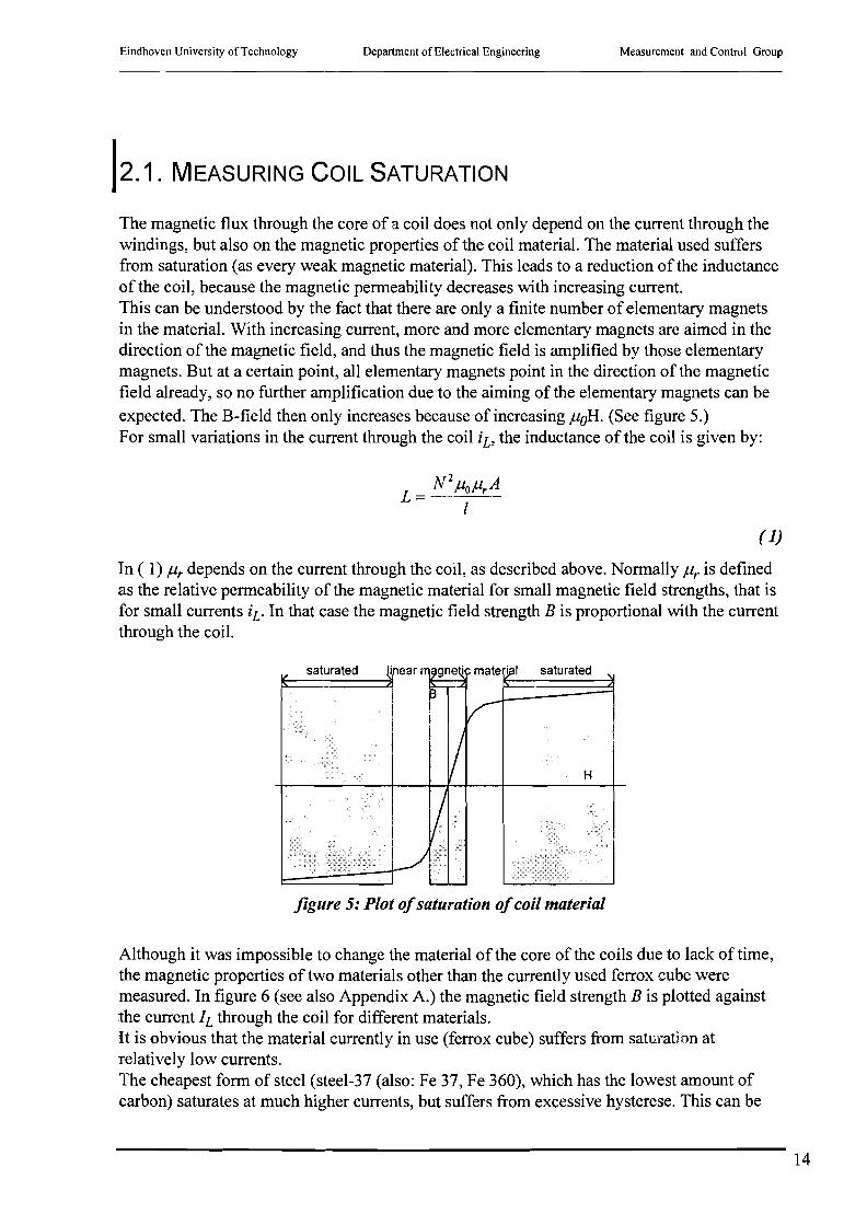
The magnetic flux through the core of a coil does not only depend on the current through thewindings, but also on the magnetic properties of the coil material. The material used suffersfrom saturation (as every weak magnetic material). This leads to a reduction of the inductanceof the coil, because the magnetic permeability decreases with increasing current.This can be understood by the fact that there are only a finite number of elementary magnetsin the material. With increasing current, more and more elementary magnets are aimed in thedirection of the magnetic field, and thus the magnetic field is amplified by those elementarymagnets. But at a certain point, all elementary magnets point in the direction of the magneticfield already, so no further amplification due to the aiming of the elementary magnets can beexpected. The B-field then only increases because of increasing ,uoH. (See figure 5.)For small variations in the current through the coil iL , the inductance of the coil is given by:
N 2,uo,ur AL =---'--".'-'--
I
( 1)
In ( 1) ,ur depends on the current through the coil, as described above. Normally,ur is definedas the relative permeability of the magnetic material for small magnetic field strengths, that isfor small currents iL. In that case the magnetic field strength B is proportional with the currentthrough the coil.
saturated
H
figure 5: Plot ofsaturation ofcoil material
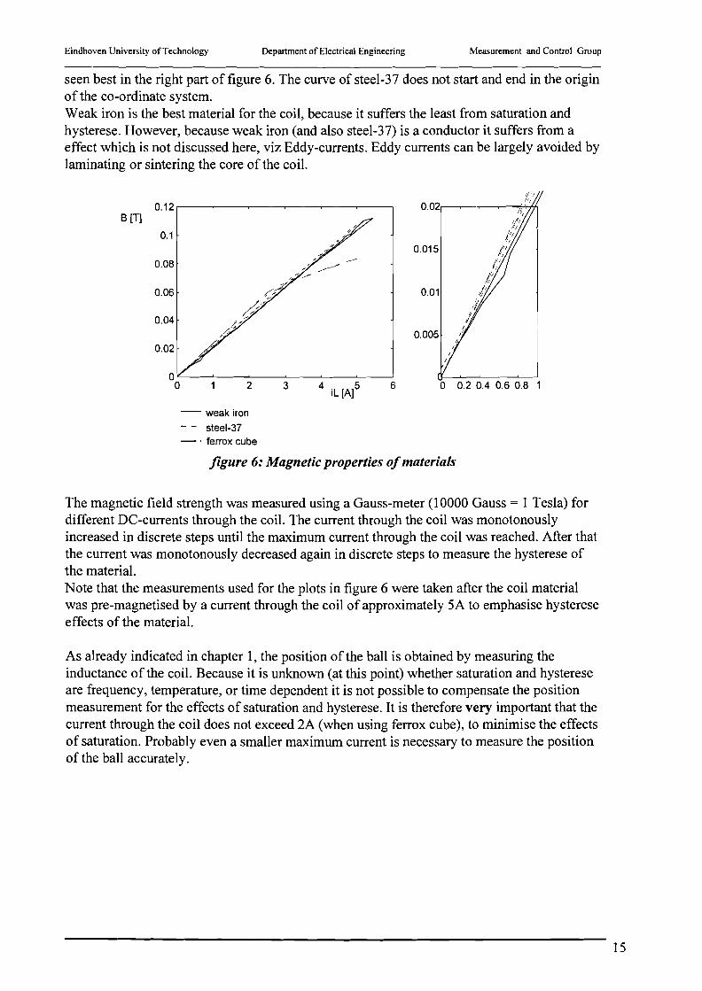
Although it was impossible to change the material of the core of the coils due to lack of time,the magnetic properties of two materials other than the currently used ferrox cube weremeasured. In figure 6 (see also Appendix A.) the magnetic field strength B is plotted againstthe current h through the coil for different materials.It is obvious that the material currently in use (ferrox cube) suffers from saturation atrelatively low currents.The cheapest form of steel (steel-37 (also: Fe 37, Fe 360), which has the lowest amount ofcarbon) saturates at much higher currents, but suffers from excessive hysterese. This can be
14
Eindhoven University of Technology Department of Electrical Engineering Measurement and Control Group
seen best in the right part of figure 6. The curve of steel-37 does not start and end in the originof the co-ordinate system.Weak iron is the best material for the coil, because it suffers the least from saturation andhysterese. However, because weak iron (and also steel-37) is a conductor it suffers from aeffect which is not discussed here, viz Eddy-currents. Eddy currents can be largely avoided bylaminating or sintering the core of the coil.
0.12B [Tj
0.1
0.08
0.06
0.04
0.02
00 2
- weak iron
- - steel-37- . ferrox cube
3 4 iL [Aj56
0.015
0.01
o 0.2 0.4 0.6 0.8
figure 6: Magnetic properties o/materials
The magnetic field strength was measured using a Gauss-meter (10000 Gauss = 1 Tesla) fordifferent DC-currents through the coil. The current through the coil was monotonouslyincreased in discrete steps until the maximum current through the coil was reached. After thatthe current was monotonously decreased again in discrete steps to measure the hysterese ofthe material.Note that the measurements used for the plots in figure 6 were taken after the coil materialwas pre-magnetised by a current through the coil of approximately 5A to emphasise hystereseeffects of the material.
As already indicated in chapter 1, the position ofthe ball is obtained by measuring theinductance of the coil. Because it is unknown (at this point) whether saturation and hystereseare frequency, temperature, or time dependent it is not possible to compensate the positionmeasurement for the effects of saturation and hysterese. It is therefore very important that thecurrent through the coil does not exceed 2A (when using ferrox cube), to minimise the effectsof saturation. Probably even a smaller maximum current is necessary to measure the positionof the ball accurately.
15

Eindhoven University of Technology Department of Electrical Engineering Measurement and Control Group
12.2 MEASURING SMALL-SIGNAL COIL PARAMETERS
Because saturation (see previous section) must be avoided, the currents applied to the coil arerelatively small. The small signal coil parameters can be measured very accurately using asimple ohm-meter and an inductance-meter. The inductance is measured when the distancebetween the ball and the coil is infinitely large. The results can be found in table 2.
Resistance [Q] Iriductance [mR]Upper coil 3.570 108.70Bottom coil 3.409 111.10Left coil 3.406 107.12Right coil 3.465 106.80Gravity coil 4.720 109.18
table 2: Small signal coil parameters
The values in table 2 show the great similarity between the five coils. The inductances andDC-resistances are about all the same, except for the gravity coil. Its DC-resistance is muchhigher than that of the other four coils. This can be explained by the fact that the gravity coilis winded around the upper coil, so that the radius of the windings is larger and the totallength of the wire is longer.Although the position of the ball is obtained by measuring the inductance of the coil, the exactvalue of the inductances in table 2 is not interesting. The position of the ball is cal.culated bymeasuring the deviation of the inductance from the value in table 2.
12.3 MEASURING POSITION I INDUCTANCE RELATION
The relation between the position of the ball and the inductance of the coil is depicted infigure 7. See also appendix B. Measurements were made by measuring the inductance of thecoil with an inductance-meter for different distances between the ball and the coil.
When an inverse proportional model is fitted on the measurement data, using a vertical leastmeans square method, the result is a model that does not describe the behaviour of the processvel)' well. (This will be discussed in detail in chapter 3.) So an exponential model is used forthe process. ( 2)Because the vertical least mean square method was used to fit the model on the measurementdata, most data points were chosen around the steady state operating point of the system(x=0.005 [m]) , and only a few with larger distance between the coil and the ball. Thereforethe model is not fitted very well on the data for larger distances between coil and ball.
16

Eindhoven University of Technology
Lm(mH)
4.
2.
2
1.
1
O.
Department of Electrical Engineering
LMS-fit: Lm=A*exp(-B*x)
Measurement and Control Group
o 0.005 0.01 0.015 0.02 0.025 0.03 0.035x(mm)
figure 7: Position / inductance relation
The values Ls, A and B found for the for the process are:
L = L + A .e- B.xs
L., =102.89[mH]
A =4.941[mH]
B =138[m-1]
(2)
Note that Ls in (2) does not comply with Ls in table 2. This is because Ls can changesignificantly when the amount of magnetic material in the direct environment of the coil ischanged. However, because exact value of Ls is unimportant, Ls will be approximated by thevalue O.11H.
Note that the relation between the induction of the coil and the distance between the ball andthe coil is measured when the ball moves in the vertical direction only. Variation in inductionby horizontal displacement is not measured. This means that the levitation system will be onedimensional.
17

Eindhoven University of Technology Department of Electrical Engineering Measurement and Control Group
/3. THEORY OF MAGNETIC LEVITATION
In this chapter the equations of a magnetic levitation system are derived. For simplicity, theball is assumed to move in the vertical direction only. This means that the coils for horizontalmovements are assumed to be absent, and thus have no influence on the ball.When the position of the ball must be controlled in two directions, the relation between theposition of the ball and the inductance of the coil (figure 7), must be measured in twodimension. Furthermore, the magnetic reluctance force (as will be derived in the chapter)would be a function of the vertical as well as the horizontal position of the ball. Also, the(varying!) mutual coupling between the coils influences the magnetic reluctance force and therelation between the position of the ball and the inductance of the coil. This would complicatethe system very much. Therefore only the one dimensional levitation system is examined inthis thesis.
The coils can be operated in two different ways. The first is to apply a certain voltage over thecoil (voltage control) by a voltage source, the current through the coil is then given by theimpedance of the coil, according to:
( 3)
In formula ( 3) ir is the current through the coil, Vr is the voltage over the coil, L is theinduction of the coil and Rr is the serie resistance.
The other way to control the coil is to force a certain current through the coil (current control)by a current source. The voltage over the coil is then given by:
( 4)
In this chapter the relation between the current through the coil and the position of the ball aswell as the relation between the voltage over the coil and the position of the ball are derived.After that, those relations are linearised in an operating point of the process to calculate thelinearised transfer function of the one dimensional levitation system.
13.1 DERIVATION OF THE COIL EQUATIONS
In this section the equations of the one dimensional magnetic levitation system are derived.The symbols as in figure 8 will be used.
18

Eindhoven University of Technology Department of Electrical Engineering Measurement and Control Group
iL
~llUL S
~L
~ Jfigure 8: One dimensional levitation system
In figure 81m is the magnetic reluctance force exerted by the coil on the ball,lg is thegravitational force, m is the mass of the ball, x is the distance between the coil and the ball, RLis the DC-resistance of the coil and L is the inductance of the coil, iL is the current through thecoil and VL is the voltage over the coil (serial connection of the inductance L and itsresistance RL).
In most literature about magnetic levitation (e.g. [1], [5], [8], [10], [11] and [12]) it is assumedthat the number ofmagnetic flux lines running through the ball does not depend on the'distance between the ball and the coil. However, this is not true for the physical process usedfor this report. (See also section 2.3.)Nevertheless we can easily set up a derivation based on the assumption that the number offlux lines through the ball is independent of the position of the ball. When further assumedthat:• The flux lines through the coil have only two paths: One path from one end of the coil
directly to the other. The other path is from one side of the coil, through the ball, to theother side of the coil.
• The permeability of the material of the coil and ball is infinite large, and does not dependon the amount of flux lines through it. (No saturation)
• The material of the coil has no memory effect. (No hysterese)• The permeability of air is one.
the relation between the coil inductance and the position ofthe ball can be derived usingHopkins' law. [13] This leads to [10], [11], [12]:
<I> f.lvAN 2
L=-=L +L = +LiL
m s (X + 2x) s
(5)
In ( 5) cP is the magnetic flux, iL is the current through the coil, Ls is the inductance ofthe coilwhich does not depend on the position of the ball ('parasitic inductance'), Lm is the positiondepended part of the inductance of the coil, X is a constant depending on the geometry, A is aconstant depending on the geometry, N is the number of windings on the coil and x is thedistance between the ball and the coil.Formula ( 5) shows that the inductance should be inversely proportional to the position of theball. However, when the constants X and A were fitted on measurements of the real process asobtained in chapter 2 with a vertical least mean square fit, it was clear that the modeldescribed in ( 5) was not a good description of the process. (See figure 9.)
19

Eindhoven University of Technology Department of Electrical Engineering Measurement and Control Group
Experiments with different models have shown that the relation between the inductance of thecoil and the position of the ball is best described by:
L = L + A .e-B·;r.\'
(6)
Lm[mH]LMS-fit: Lm=N(B+x)
0.005 0.01 0.015 0.02 0.025 0.03 0.035x[m]
4.
3.
2.
LMS-fit: Lm=A*exp(-B*x)
0.005 0.01 0.015 0.02 0.025 0.03 0.035x[m]
figure 9: Vertical least mean squarefits on coil measurements
A physical explanation of the exponential model ( 6) is that the pattern of the magnetic fluxlines of the coil is best depicted in figure lOb rather than in figure lOa. The closer the ball is tothe coil, the more flux lines run through the ball. Above experiments show that this relation isapproximately exponential for the process under study.
'------',----' a
figure 10: Flux lines through coil and hall
The magnetic reluctance force1m by the coil in the quasi-static situation (that is, when thekinetic energy of the ball is small) can be calculated using the law of energy conservation:When the current through the coil is held constant, any variation in the energy of the magneticfield is due to movement ofthe ball. This leads to: [13]
20

Eindhoven University of Technology Department of Electrical Engineering Measurement and Control Group
dW (<1> X) = i . d<1>} OW OWm' L => i . d<1> _ r .dx = dW (<1> X) = __m d<1> + _III dx
dW (<1> ) = r .dx L J m m' at> de", ,X Jm
- OW (<1> X) !i".mag1l.malerial 1 dL 1 d ( ) 1/,
m' ·2·2 L A -B·x AB -B·x ·2= = -I -=-1 - +'e =-- ·e '1", de 2 L dx 2 L dx of 2 L
(7)
where C/J is the magnetic flux Wm is the magnetic field energy andfm is the magneticreluctance force.
Remark that the partial derivation - OW~<1>,x) in ( 7) means that the magnetic field energy
must be differentiated with respect to X when C/J(and so iL) is held constant. So the magnetic
1 dL 1 d( ii .L)reluctance force is given by 1", =2ii dx and not by 1,,, "* 2 dx . [13]
The voltage over the coil, given a certain current iL through the coil is given by:
(8)
It is assumed that the ball moves in the vertical direction only, so the dynamic equations of theball can easily be derived using Newton's second law.
(9)
Combining ( 7) and ( 9) gives a relation between the current through the coil iL and theposition of the ball x:
Id2X
1,,, =m-2 - f g
dt => mx - f. = _lPABe- BX
1 g 2 L/, ·2 AB -Bx"'=-2IL e
( 10)
When formula ( 10) is combined with ( 8), it gives a relation between the voltage over the coilVL and the position of the ball x.Obvious, the relations between current and position or voltage and position are not linear.However they can be linearised in an operating point (xo, iL,O) respectively (xo, VL,O) using theTaylor approximation. In this manner the linearised transfer function of the system can bederived. First this is done for current control, after that the transfer function of the voltagecontrolled system is derived.
21
Eindhoven University ofTechnology Department of Electrical Engineering Measurement and Control Group
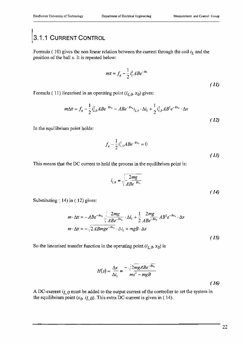
3.1.1 CURRENT CONTROL
Formula ( 10) gives the non linear relation between the current through the coil iL and theposition of the ball x. It is repeated below:
1 .2 -BxmX =J. - - 1 ABeg 2 I,
( 11)
Formula ( 11) linearised in an operating point (iL,O' xo) gives:
( 12)
In the equilibrium point holds:
1f. - - i2 ABe- Bxo =0
g 2 L,a
( 13)
This means that the DC current to hold the process in the equilibrium point is:
. !2mg11,,0 =~ ABe- Bxo
( 14)
Substituting ( 14) in ( 12) gives:
~---
m.t1X=-ABe-Bxo I. 2mg .f).i +! 2mg AB2e-Bxo.&~ ABe-1Jxo I, 2 ABe-Bxo
m· t1X =-fiABmge- liXo . f1i" + mgB· &
( 15)
So the linearised transfer function in the operating point (iL,O. xo) is
H(s) = ~_ = - {27gABe-BXof).1I, ms - mgB
( 16)
A DC-current iL,°must be added to the output current of the controller to set the system inthe equilibrium point (xo. iL,O). This extra DC-current is given in ( 14).
22

Eindhoven University of Technology Department of Electrical Engineering Measurement and Control Group
When ( 16) is factorised the following relation is obtained:
x(s) ~2ABge-Bx" 1H( s) = i(s) =- m (s-+--JgB-gB~)(-s--J&-----=gB==-)
( 17)
One can see that poles of the linearised transfer function are independent of the linearisationpoint xo. Only the gain of the linearised transfer function depends on the linearisation point.This is only true when for the relation between the position of the ball and the inductance ofthe coil an exponential model is used.
One other point of attention is that the gain of the linearised system is negative. Whendesigning a controller for the system, one has to be careful to not to generate a positivefeedback, instead of a negative.
A pole zero map of the current controlled system will be displayed in chapter 7, when acontroller is designed for the system.
3.1.2 VOLTAGE CONTROL
Formula ( 10) gives the non linear relation between the current through the coil iL and theposition of the ball x; formula ( 8) between the voltage over the coil UL, the current throughthe coil iL, and the position of the ball x. They are repeated below:
( 18)
The bottom relation of formula ( 18) linearised in an operating point (UL 0, xo) gives:,
U AU - R' R A' (L A -BX,,) A' • AB -Bx" A.~L,O + Ll L - L' lL,O + L' LllL + S + e . LllL - lL,O e . L.U
( 19)
In the equilibrium point holds:
(20)
23

Eindhoven University of Technology Department of Electrical Engineering Measurement and Control Group
Substituting ( 14) in (20) gives the DC-voltage over the coil necessary to hold the process inthe equilibrium point. The DC-voltage is:
VL,o =RL • iL,o
V - R. 2mgL,O - L ABe-Be<o
(21)
Substituting (14) in (19) and using (15) gives:
/).V = R . /).i + (L + Ae-Be<o). /).; - i ABe-Be<o.!:rtL L L.. L L,O
V R mgB·!xx-m·Ax (L A -Bx ) mgB·!:rt-m·/),% ~I 2mg AB -Be< ./). = . + + eO. - e II·ML L -J2ABmge-Be<o s -J2ABmge-Be<o ABe-Be<o
( 22)
So the linearised transfer function in the operating point (VL,O' xo) is:
(23)
A DC-voltage VL 0 must be added to the output current of the controller to set the system in,the equilibrium point (VL, 0, xo). This extra DC-voltage is given in ( 21).
When (23) is factorised the following relation is obtained:
(24)
\Vhen looking at the linearised transfer function of the voltage controlled system, oneobserves that the poles of this system are simply those ofthe current controlled system, with
one additional pole of the resistance Iinductance serial connection. (s + R/(L, + Ae-Be<II))
Only the position of this additional pole depends on the linearisation point xo. The gain of thelinearised transfer function also depends on the linearisation point.One other point of attention is that the gain of the linearised system is negative. Whendesigning a controller for the system, one has to be careful to not to generate a positivefeedback, instead of a negative.
24

Eindhoven University of Technology
13.2 CONCLUSIONS
Department of Electrical Engineering Measurement and Control Group
In the previous section the linearised transfer functions of the one dimensional magneticlevitation system were derived for both current controlled coils and voltage controlled coils.
When examining the differences in the two linearised transfer functions, one can see that fromthe point of view of the controlling of the levitated ball, the current controlled coil is the mostattractive, because its transfer function is only of the second order. Further on, the poles of thelinearised transfer function of the current controlled system do not depend on the linearisationpoint. Only the gain of the transfer function depends on the linearisation point.In the next chapter will become clear that from the point of view of the actuator currentcontrol has some disadvantages. (See chapter 4.)
25
Eindhoven University of Technology
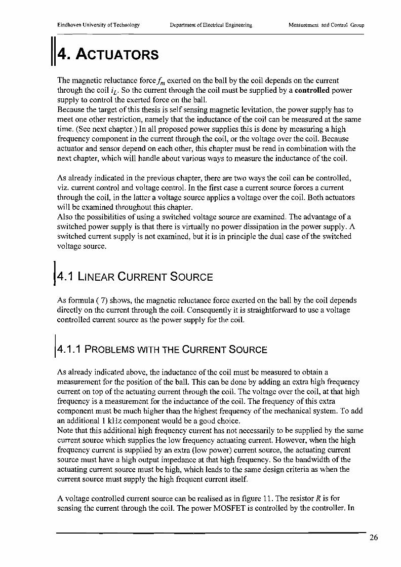
4. ACTUATORS
Department of Electrical Engineering Measurement and Control Group
The magnetic reluctance force1m exerted on the ball by the coil depends on the currentthrough the coil iL' So the current through the coil must be supplied by a controlled powersupply to control the exerted force on the ball.Because the target of this thesis is self sensing magnetic levitation, the power supply has tomeet one other restriction, namely that the inductance of the coil can be measured at the sametime. (See next chapter.) In all proposed power supplies this is done by measuring a highfrequency component in the current through the coil, or the voltage over the coil. Becauseactuator and sensor depend on each other, this chapter must be read in combination with thenext chapter, which will handle about various ways to measure the inductance of the coil.
As already indicated in the previous chapter, there are two ways the coil can be controlled,viz. current control and voltage control. In the first case a current source forces a currentthrough the coil, in the latter a voltage source applies a voltage over the coil. Both actuatorswill be examined throughout this chapter.Also the possibilities of using a switched voltage source are examined. The advantage of aswitched power supply is that there is virtually no power dissipation in the power supply. Aswitched current supply is not examined, but it is in principle the dual case ofthe switchedvoltage source.
\4.1 liNEAR CURRENT SOURCE
As formula ( 7) shows, the magnetic reluctance force exerted on the ball by the coil dependsdirectly on the current through the coil. Consequently it is straightforward to use a voltagecontrolled current source as the power supply for the coil.
4.1.1 PROBLEMS WITH THE CURRENT SOURCE
As already indicated above, the inductance of the coil must be measured to obtain ameasurement for the position of the ball. This can be done by adding an extra high frequencycurrent on top of the actuating current through the coil. The voltage over the coil, at that highfrequency is a measurement for the inductance of the coil. The frequency of this extracomponent must be much higher than the highest frequency of the mechanical system. To addan additional 1 kHz component would be a good choice.Note that this additional high frequency current has not necessarily to be supplied by the samecurrent source which supplies the low frequency actuating current. However, when the highfrequency current is supplied by an extra (low power) current source, the actuating currentsource must have a high output impedance at that high frequency. So the bandwidth of theactuating current source must be high, which leads to the same design criteria as when thecurrent source must supply the high frequent current itself
A voltage controlled current source can be realised as in figure 11. The resistor R is forsensing the current through the coil. The power MOSFET is controlled by the controller. In
26
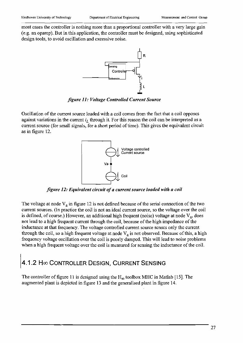
Eindhoven University of Technology Department of Electrical Engineering Measurement and Control Group
most cases the controller is nothing more than a proportional controller with a very large gain(e.g. an opamp). But in this application, the controller must be designed, using sophisticateddesign tools, to avoid oscillation and excessive noise.
ensing
Cantrall
R
L
figure 11: Voltage Controlled Current Source
Oscillation of the current source loaded with a coil comes from the fact that a coil opposesagainst variations in the current iL through it. For this reason the coil can be interpreted as acurrent source (for small signals, for a short period oftime). This gives the equivalent circuitas in figure 12.
,I Voltage controlled~ Current source
figure 12: Equivalent circuit ofa current source loaded with a coil
The voltage at node Vain figure 12 is not defined because of the serial connection of the twocurrent sources. (In practice the coil is not an ideal current source, so the voltage over the coilis defined, of course.) However, an additional high frequent (noise) voltage at node Va' doesnot lead to a high frequent current through the coil, because of the high impedance of theinductance at that frequency. The voltage controlled current source senses only the currentthrough the coil, so a high frequent voltage at node Va is not observed. Because of this, a highfrequency voltage oscillation over the coil is poorly damped. This will lead to noise problemswhen a high frequent voltage over the coil is measured for sensing the inductance of the coil.
4.1.2 Hoo CONTROLLER DESIGN, CURRENT SENSING
The controller of figure 11 is designed using the Hoo toolbox MHC in Matlab [15]. Theaugmented plant is depicted in figure 13 and the generalised plant in figure 14.
27

Eindhoven University of Technology Department of Electrical Engineering Measurement and Control Group
w G Z
V11 sensor noise
system noise tracking W11V22
f'fIference emPIre-V33
~iJ- I~ + erroru +....'~ vtJ I·~
,p vO
<iI
Controller
.C
figure 13: Augmentedplant
controller
w
figure 14: Generalised plantfor MHC-Toolbox
In figure 13 the plant P is the MOSFET, the coil L and the resistor R of figure II. The input ofthe plant is the voltage at the gate of the MOSFET vb the two outputs of the plant are theoutput current iL and output voltage of the current source va (when loaded with the coil).Although the current through the MOSFET is given by a non linear relation with the gatesource voltage, the plant is assumed to have a linear transfer function. (Any non linearity ofthe process is eliminated by the enormous gain of the controller. See further on)As resistor R is assumed to be IQ, the transfer function P11 is 1 [AN], which means that IVat the gate of the MOSFET gives IA through the coil. Transfer function P I2 is given by theinductance of the coil and its serie resistance. ( 4) An extra pole at an unimportant highfrequency is added to the zero, to make transfer function P I2 bi-proper. This gives:
R _ I10s+ 3.512 - 0.0159s + I
The plant has three exogenous inputs. The first is the sensor noise, with its shaping filter VII'lt is assumed that the signal to noise ratio of the current sensor (and its additional electronics)is 40dB at all frequencies. This means that ~ I =-40dB =0.0 IThe second exogenous input of the plant is system noise, with its shaping filter V22 . Systemnoise is for modelling the noise of the electronics of the controller. The signal to noise ratio of
28

Eindhoven University of Technology Department of Electrical Engineering Measurement and Control Group
the electronics of the controller is assumed to be 40dB at all frequencies. This means that~2 = -40dB = 0.01The third exogenous input of the plant is the reference signal, with its shaping filter V33' Thereference signal is shaped by V33 in such way, that the current source is able to supply thedemanded current, at all frequencies. (This means that the output voltage of the current sourcedoes not exceed the supply voltage of the current source Vdd, which is 30V). An additional
. .. 0.055s + 3.5zero is added to make V33 bi-proper. This gives for V33 : ~3 =---35
11 Os + .Note that weighting filter V33 as state above does not guarantee that the input signal of thecurrent source is small enough to avoid saturation of the current source. It only gives an roughestimation of the input signals of the current source for designing the HOC) controller for thecurrent source.
Further on it is assumed that: IlwJ2,llw2112,lIwJ2 < 1
The generalised plant has two exogenous outputs. First of all the tracking error, with itsshaping filter W11 . This filter is designed in such way that tracking errors for smallfrequencies and tracking errors at the position measurement frequency are weighted heavily.
. . 18.7S3 + 1229s2 + 3445s + 2469. . .ThiS gives for Wn : ~1 = 3 2 • In thiS way the weightmg upon
s +13.88s +4732s+24.76tracking errors in the interesting frequency bands is 40dB (This gives a tracking error of10..30mA) It is not possible to increase weighting on tracking errors, because the sensor noiseis only -40dB. Again the weighting filter is made bi-proper by adding an additional zero at anunimportant (high) frequency.The other exogenous output is the output voltage of the current source with its shaping filterW22. The maximum output voltage of the current source is bounded by its supply voltage Vdd,
which is 30V. This means that W:z2 =0.0333Note that (as with all other signals which are bounded to certain value in the time domain)weighting filter W22 gives no guarantee that the output voltage of the current source neverexceeds 30V.
Finally it is assumed that: Ilzlli2,llz2112 < 1
Note that all transfer functions are bi-proper, which means that the order of the numeratorpolynomial is equal to the order of the denumerator polynomial. This is necessary whencalculating an HOC) controller because else the weighting on very high frequencies would bezero or infinite (depending on the transfer function). This would give incorrect answers. Forthis reason extra poles or zeros are added (at very high, unimportant frequencies) to eachtransfer function to make them proper. The transfer function of the process P12 is proper too,which means that an additional high pass filter must be added parallel to the coil so that thesimulations agree with practice. (See section 4.1.4.)Note that all frequencies are expressed in krad rather then in rad, to avoid numerical problemswhen calculating the HOC) controller
The transfer functions of the plant and the weighting filters are repeated below:
29

Eindhoven University of Technology Department of Electrical Engineering Measurement and Control Group
~I =1
P. _ 110s + 3.512 - 0.0159s+1
J!;1 =0.01
V22 =0.01
0.055s+ 3.5J!;3 = 110s + 3.5
18.7s3 + 1229i + 3445s + 2469~l = S3 +13.88i + 47.32s+ 24.76
~2 =0.0333
(25)
The transfer functions of the plant and the weighting filters are plotted in figure 15.
11I111
111I111
111111
1111,:1
_ L L U I.J.IU
I 1111"1'
I II111111
I 1IIIIIIi
\ 11II1111
P12
100 101
Frequency kradV33
10-1
'111'1' 1111111 II !IIII I 1111111
I i I 'II '11111 1111111 I 1I11111
I IIIII! I I 1111111 I111111 I 11111',1
I 11111111 I I 111111 I 1111111 I 1111111
_1_ U-1Il..!I:- _ L' 1...lllllL _ L LI.J !.J.lll _ L 1 U UI
111111: I 1I11I I 1111111: I 111I1I1
I I lilli' I I I II 1\ I 111111!i I I; I illl
I 1111I1 ! 11111' I I I11I11I
I 111'111 I I 11111I1 I I111111
_1_ U -1IUIL _ L L1..lI-111l _ L _ L L U UI'
I 11111111 I I I111111 I I I
I I 1111111 I I II11111 1
I 11111111 I 11111111
I I I III HI I I 111111
_1_ U -1IUIL _ 1_ LU 1-111.1
I 1111111' I I lilli'
I I 1111111 I I 111III1
I I1I1I1I1 I I 1111111
I 1111[11' ! I I 111111
o
I I IIII!II I I I illill 1111!li I111111
'111111 1111111 'II 111111
'111i'l I I 1111111 Ilill" 1111I11
I111111 I I IIIII!I I I!, ,'''1 I I' .11
-1- 1-'1('1111 - f T 1-11-1111 - 1 I TIII:I'- 11-11:1
I 1111I11 I I I 111111 I 1111111' I 111II1
I 11111',1 I I I1111I1 I 1111111' I 1111'111
I I 11II111 I I 111111I I II il! I I1I1111
I 1'11111 : I I I 11111 I 1111111
I I II I· II 1111:11'- -1-111-1111
I 1111[11 1'11'11 I ,111
I I I lilli' I 111111' I 11'1111
I 11111111 I 1IIIIIi' 111111
_1_ ~[J Ilill _ 1.- _IIJI.!...I _ J. J .!..I...!..I~' __, _I J I...,! IJ.I
I I 1111111 I 11I11111 I 11111I1
I I I I11111 I 1111111 I 111'111
I I I III' I I 1111111 1',11111
I I 11\1 I I IIIIII! I111111o10-2
20
40
-40
-60
dB-20
80dB
60
I I1IIII1I I llll,;
I I l'lllil rl1111 I !IIIII
I1III111 I I Ililll IIIIII1
I I !Iilll I I Il,illl I IIIIII11
I Ii IIIII1 1'111111\ I IIII111
-1-ITITlln - r ,'TlrT:l- 11 nnirr
I Illillll I IIIIII11 '\111111
I 11111111 I I illlill I I III
IIIII11 I 11111111 IIIII11
IIIIIII1 IIIII11 I 1;11111
P11
Illilll I IIIII!I: I
111"1111 I I1III11 I
I IIIII11 1'1 !IIIII I
I IIIII11 I I IIIII11 I
__I J. I.!...I IJ..! _ ~ ~ I .!...I II I III I I
I IIIIII!I I
IIIII11
III1111
,. . . ".I I I 1'1111 I I I IIIIII I I IIIII11 I I IIIII1
I I I III I 11 I, I 111111 I I IIIII11 I I IIIII1
I I 1111111 I I I IIIII1 I I 1IIII11 I I 111111, , i III111 I I ,
"
II I , , II1I11 I , IIIII1_.I- , , 1111:1 - - -
I-
I IIIIII1- - ,- IlllllI I
, I ,llliil I I , 1111,1 , I Illllil , I lillI',
I I lillI'" I I I 1'111 1 i , I111111 I 1111I1
I I , 1111I1 , I I 111111 , 111111 1 , I '1,111
I I 111111 I I , :111'1 I !IIIII , I 111111
I I , 1I1111 I I I 11,'11 , I 1111111 , I I11111
I I , 111111 I I 11,,11 I 1IIIili I I 111111
I i I1I1111 I I , 111111 I 111111' I I I11I1I, 1111111 I , 111111 I , 11\1111 I , 11I111
- I - I llJ.llJ.! - C. !-. !...!. I.!..! "- _.,
-, Jllll.!..1 - C. C. 1J.llJl, i 1IIIil I , , 111111 I , 1111I11 I , 111I11
I I 11 11111 , , I 1111I1 , I 111I111 I I 1(1111
I I 11'1111 , I I 1I11I1 I IIIIII! I lilli',
I I I11I11 I I , 1111I1 I IIIIII! , ,I ~ " :: I
-2 -1 ,0 \1-41
10 10 10 10Frequency krad
1
-40
o
-0.5
-40.5
-39
dB-39.5
dB0.5
30

Eindhoven University of Technology Department of Electrical Engineering Measurement and Control Group
IIIIIII1III11
IIII!I
I III11I1
- I I" \11111I j Ililil
I IIIIII1
I i I ilill
Illllll 11III11
11111111 I 1111111
11111111 I 1111111
t- 1""1 1+1 It- - r- t- H r+ I
11111111 I 111111'
11111111 I 1111111
I I11111I I 1111111
1-14 1..l.1~ _ j.... +-I~ L-I-I
11111111 I 1111111
11111111 I 1111111
11111111 I I1111I1
W22I I IIIII1 IIIIII11
I IIIII11 I I1IIII1
I IIIIII1 111111',
, IIIII11 IIIII11- - 1-1111111 - - -1111111
I 11111111 I IIIIII11
I 111111',1 I IIIIII11
I I IIIII11 I II1IIII1
-30
-30.5
-28.5 , IIIII11
IIIII I 1 dB, II I III1
111',11 , ,"
IIII
I ilill -29 ' , ,
, IIIII1- - I-
I
IIIII1 I , IIIIII1
III1I1, i I1III1
flTI II -29.5, 1,11111
W11I ,1111111 IIItl1
I I illill I I 11'111
Illillll I 111'111
I IIIII11 IIIIII11
1IIII11 III11I1 I \
Ii 1,111; I I I 'III' Ijllill
-I-Ii 11',rr:- T T i1rT:rT -1~1-lnrTI1-
I Ii 11111t ; II I l'llllli
I 1IIIIIil \ I I I11II1 I III1III1
I II11I1 1'11,1,1 IIII111 I
I I IIIII11 I lilli" I Illillll I
I IIIII!II I IIIIII1 I I IIIII11 I
I I I I IIIII11 I 111I I 111 I I------------1 I 11111111 111\111 I
I I I i I I I I I I I I ~ I 1 I I I I I
I !IIIII 111111II 1111111
Illillll 11111111 1111111
I 11II1111 I1I1111 111I111
I 1I1111I1 1111111 1111111
1111111 I 1I111111
I I 1111\11 I 11I11111
I I 1111111 I 111I1111 I
-1-1-1+1t-i1t- - f- \-1+ITiIt- -.-
I I 1111111 I 111\1111 I
I 11111111 I I11I1111 I
I I I1I1111 I I I I1I111 I
_1_1_1..l-1-I-J 1>-.-_I--I--I-l-I-l-II+-_1-
I I 1111111 ! I 11I1111 I
I I 111I11I 11111I11 I
I 11111111 I 1111111 I
-3110-2 10-1 100
Frequency krad Frequency krad
figure 15: Weightingfiltersfor MHC-Toolbox
30
2510-
40
dB35
When a controller is designed using the weighting filters as in ( 25) the Hoo toolbox for MatlabMHC gives the results as in figure 16. The solid line is the transfer function from a certaininput of the augmented plant to a certain output. The dashed line is the boundary of
guaranteed stability (when y is equal to 1). The optimum ywas found to be 0.998, which isclose to 1, as it should be.
Controller Closed Loop Tracking Error (3->1)50 r-,..-,nrrm-~TTrTTT''-----T""TTTTmr----r"TTrrrm
1'111:
1111111
"III
I 1'1'11
'III: '1111111 I 11111111 I I II [III
: I I I III I I I I III; I I I I I 1I1I I I I vrfi I
11111111 I I I111I1 I 11111111 I --rl11111
11I1111 11111111 111111111 A I111I11
11111111 I 11111111 I 111'1l,.H'1 I 1111111
_1_'-' LII_~II __ 1_1-.1 UI~II_ :;d--1..:t1.J11lI- J...J 1..1.111
! I I I I I 'II I I I I I I r '-:'..-'-'-",-",J..I"-""-"_-'-~~.,Illt~:1 [I Iylill I I111I111 I 11I1111
1'11:1' [....-'"1"1'1 II 111111111 11111111
IIIIIIII~II 1111I 11I111111 111I1111
I...-l-I~III I 1111111 I 1111111 11111111
1111111 I 1'1111111 I 11I1111
-I-'I r r-; -I-Ii n,T11- ~I-I 11111'""11-"""'" TIT:
I I 1111111 I I 1I1I111 I 1111111
I 11111111 11111111 I I111111
I I; 111111 I I111I11 I I 11'1111
111',111 11111111 I 111111
1111111 11111111 I 1I1111
o
-50
dB
I 11111!1
I Ii Ilill
11I111
J -' C.::...! I~
I I , "1111 , , ~ I _I ,, I ! illl , , , , , ' 1' ,1, I , 1111I1 , , , 11',11" ,11111
11111:.1
i I11II1
I 111111 I I' I I "I, I I I I q
1111111 '111111 11111,1
11,11111 I I: lilli' 1111,,1 i 11111
nlnl- 1 -r nnl;j - r rITIT1i: -"-'i n:II 'I' I ,'"11,1 111111I1 I Ill!111
1IIIIi I1I1111 I 11111111 I Illil\1
I IIilll1 I 11I1I 11 1 I 11I11111 I 1I11111-I-,I llilil - I II nlf] - 1- 1-,111111- -1-11,1111
I I11I1111 I 1111111 I111111 I 1111111
I \ II1I111 I I 11111 11>\111 I 111I1II
I I I11111 I I 11'111 I 11111 1, I 11111111IIIiI:-II-liI,- - 1- -1--111111
I 11111111 I 11111111 111111
1111111 I 1'111'11 1I1111
_'_IJ IJIiJ.I_o
40
20
10-' 10° 101
Frequency krad
-1 00 '------'---'--'---'-'.wL--"----'--'-W..J.=-----'-.L.LLllL"------'---'--L.Lll.W
1~ 1~ 1~ 1~ 1~Frequency krad
31

Eindhoven University of Technology Department ofElectricaJ Engineering Measurement and Control Group
1\1111
! 1I1I11
! I11111
:'-I.!..'ILI _ -'- ~ i_I ~II
(111;11 I 111111I
'I'll I I I 111111
,
1
1 1, ,I111I11 1111111
,ill 11I111
--' ..J ilL'!.!.! _ J... .i I_I U III 111111\1 1111
I IIIIIII! IIIIli
I I II ilili IIII!I
I 111111;, III<I!'111i
, 11111;
,111,11
11111I
I I I111I
I III!III
I Ilirlll
111I111
11I11111
I :' 1'1111
111I111
I I 1I11I11 i 1111111
I r I 1111111
! 111!llli
_'_1_11',,:,:' __i_,~I--,-IUI
_'_1_1 ~_I i~lI __1_ ..l i'
I I I 111111 I I I 11'1111
I I: 11I1I1 I I I II illl
1IIIIIIIIIIilllili
I I II 11111 I I I I II II
1111111 I 111111
1111111 I I11I1I1
I I I I I I I I I i I ~ I I I ! i I I I I I I I I I I I I I
-1-nlin!r-rrlllllrr-llr;r-,I~ - II rln
I I I illill I I 111'111 I I \ I 1I1I
1 , I II1I11 I 11111I1 I I I I11111
I I I111111 I I I I11I11 I 111IIII
I I I1111I1 I II Ililil III I I11I111
-1-1-1111111 -111111 111- InlTi-Tliillll
I I 11;1111 II11111 1I1111
I 1'1111111 111I111
I i 1111\1. 1 1111I11
_1_'_1 _ ~.!... U ~,~ ~ ~I.!...III
I I I I II illil 1IIIil
I i',1111 1111111 i :11: 1
1111111 I111111 I 1II1111
,illill 111111' I11II1
o
-50
100 r----r,"'1"""""",-,,",""'-''''II;r-",-'''''""I IT"r----r'I"""""""I I I :11111 I I I !llli' I 11111:11 i 1111111
I 111,'111 I I I111111 I 1111111 I 1,11111
I-' i""'i"Ti11-1~ 111I11-1 1"1 I \Till ------; III i"T'i'iI I III I I I I
I I III I I
I 11111111 I 1111111
O'-===t:.LLlllJJ.L.---l...LWLLlll'-----'---'-.LllWL---l..-Ll..LlllJJ
1~ 1~ 1~ 1~ 1~Frequency krad
Output voltage noise, due to system noise (2->2)
20
40
Output voltage noise, due to sensor noise (1->2)80 r-~~.....,-_~~~___r_~~~_--.-,-....",
60
dB
50
dB
, l'lli
1111:1
1111111
, ,
,
, ,
- I :
IIIIII11I I 11111:1
'11111
I 11111" I 1111',111
1111'11 1111:11
~~. I~I -=-:. ::!:--\...II'II!I!I I I II
I I',' III '..-l--,-,--'-W-,,---rrnTT11,
, , , 11',1
, ,'"
-'- '- '...:1 I.,!. - -, , , 'II
, , ,'1 1 11
, , , IIII
I III : , ,
- --I C ~ III ~ - UI'--,- -,- '- .L
"
, II!II
I ill:I'
: 1'1111 1'11111 I I
,T',I,T" - 1- 'I-I (:1 IT - T 1 rlil
I IIIIII1
I I 11,11'1
! I : ~ i I I I I
I I! 111:11-1- 1-1111111
I : :;:::: I : 1111'1 :)':: I
- i~ ~:~';~:~ - ~ +~:~::~ - t ~ +:~:';:I I IIIIII!/ I 111:111
~:~il~ : :::::::~....,......:....~~_-";;:;;;-'"-"'""'"'O-,,, - "I II II III I I IIII II
"III I I I: IIII
111'111 I: IIII
_'_ I_I....!-'ll'.!... _ ~ ~1_11J.lli
,111 1 11 1111 11
I I I ~ 1 I I I I I I I I I I I I
I IIII I I IIIIII1
0 , III!II, , Illill, , Illt!1
Output current noise, due to sensor noise (1->1)
5
-5
15
10
-1 0 L-.L....L...c.......J..llL---l---'--'L...Ll..l...lL---L..J-J-!...l.ll"----...L..J..li.l..WJ
10.2 10.1 10° 101 102
Frequency kradOutput current noise, due to system noise (2·>1)
20 ,--,-,-TTTnrr--,--,-,,.,..,,~_,_rn-TITT1-r-rTTTrm
dB
, , I i11111
dB I ,"
0, , ,
, ' ,, , , IIIII1, , I ",
-20 ", , Iii
\1'11,
II,I,
-40 - - - I IIII1-
"
i;
Iii
-60 - '!..-l i -,"
, , 1',1111, ,11111
-80 '----LL...u.L""------"--..--L~---L-'--Lc.=~'----c..L.W
1~ 1~ 1~ 1~ 1dFrequency krad
-1 00 L-.L...LJ-W.llL.---L.LL-LUliL-L-L-Ul-Wl----L-Ll..l.J..Lill
10.2 10.1 10° 101 102
Frequency krad
figure 16: Controller designed by MHC-Toolbox
The upper left plot in figure 16 shows that the designed controller has a second order low passcharacteristic in the concerned frequency band. The -6dB point is 80 at rad/sec. The controllerhas a second break point around 3 krad/sec, so frequencies higher than 500Hz have a gain ofapproximately one.The upper right part of figure 16 shows the tracking error of the output current with an appliedinput voltage. The tracking error for low frequencies is smaller than -50 dB «0.3%) However,around the inductance measurement frequency of 6 krad/sec the tracking error is as much as-10dB, which means that the output impedance of the current source is not very high at thatfrequency. This has its consequences for the sensor as will be made clear in the next chapter.The plot on the bottom left part of figure 16 shows that the output current noise damping forsystem noise is for low frequencies higher than 60 dB (>1OOOx)The plot on the bottom right part shows that the output voltage noise amplification (!) forsystem noise at the inductance measurement frequency of 1 KHz is about 40 dB (~100x) Thismeans that when the system noise amplitude is assumed to be 1 [mV], the noise in the coilvoltage at 1 kHz is 0.1 [V] (!)
The controller design by MHC is of fifth order, but can be approximated by a second ordertransfer function. ( 26)
C(s) =(s + 3000)(s +3000)
(s + 80)(s + 80)
(26)
32

Eindhoven University of Technology Department of Electrical Engineering Measurement and Control Group
Although the controller designed in this section is able to stabilise the current source when itis loaded with a coil (in contrary to a simple proportional controller), it will inevitably causenoise problems with position sensor. As already indicated, the output voltage noiseamplification is approximately 40dB. So another Hoc> controller is designed in the next section,which suffers less from output voltage noise.
4.1.3 Hoo CONTROLLER DESIGN, CURRENT AND VOLTAGE SENSING
As already indicated in the section 4.1.2, the output voltage of the current source is notobserved. Because of this, an Hoc> controller must be designed to avoid oscillation andexcessive noise. However, the controller as designed in the previous section still suffers froma system noise amplification of 40dB at the inductance measuring frequency, which is nottolerable.Therefore in this section a current source is designed, which senses not only the currentthrough the coil, but also the voltage over the coil. Minor drawback is that this leads to someadditional electronics. The controller for the current source, as depicted in figure 17, isdesigned using the Hoc> toolbox MHC in Matlab [15].
Controller
i-Sensing
------IReference
V-Sensing
R
L
figure 17: Voltage Controlled Current Source with voltage sensing
The augmented plant is depicted in figure 18 and the generalised plant in figure 19.
33
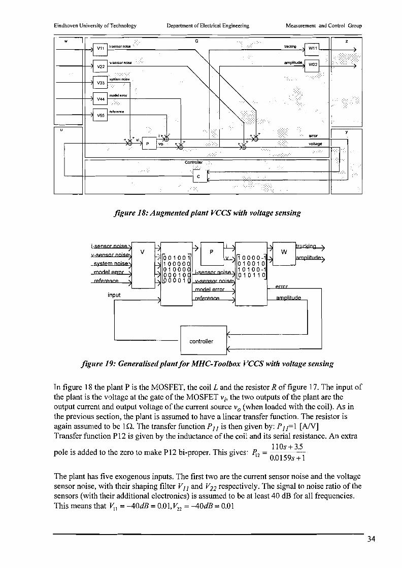
Eindhoven University of Technology Department of Electrical Engineering Measurement and Control Group
y
voltage...
G
+ + vi r---~~~-+-__---J""'="+-__I-:-*B-__,....=..,-.-_--:;9.....;rro.;...r-++----1.---++-----*&---31 + +
w
u
Controller
'---+1--------------1 C
figure 18: Augmented plant VCCS with voltage sensing
w
controller
figure 19: Generalised plant/or MHC-Toolbox VCCS with voltage sensing
In figure 18 the plant P is the MOSFET, the coil L and the resistor R of figure 17. The input ofthe plant is the voltage at the gate of the MOSFET vi, the two outputs of the plant are theoutput current and output voltage of the current source Vo (when loaded with the coil). As inthe previous section, the plant is assumed to have a linear transfer funCtion. The resistor isagain assumed to be In. The transfer function PJJ is then given by: PJJ=1 [AN]Transfer function P12 is given by the inductance of the coil and its serial resistance. An extra
I. .. . 1l0s+ 3.5
po e IS added to the zero to make PI2 bI-proper. ThIs gIves: ~2 = 00 9.15 s+I
The plant has five exogenous inputs. The first two are the current sensor noise and the voltagesensor noise, with their shaping filter VJJ and V22 respectively. The signal to noise ratio of thesensors (with their additional electronics) is assumed to be at least 40 dB for all frequencies.This means that ~ I = -40dB =0.01,V22 = -40dB =0.01
34

Eindhoven University of Technology Department of Electrical Engineering Measurement and Control Group
The third exogenous input of the plant is system noise, with its shaping filter V33. Systemnoise is for modelling the noise of the electronics of the controller. This signal to noise ratio isassumed to be alleast 40dB at all frequencies. This means that V33 = -40dB = 0.01The fourth exogenous input of the plant is the coil-model error, with its shaping filter V44 . Thevariation of the inductance of the coil because of the movement of the ball is modelled by V44.
Its value will be calculated below:Formula (2) shows that the minimum, maximum and nominal coil inductances are:
Lmin = 102.89[mH]
L"olll =105.11[mH]
Lmax =107.83[mH]
(27)
This gives a maximum coil voltage variation due to the inductance variation of the coil of:
L"OIll =1.0216LminL M max = 2.59%_max =1.0259Lnom
(28)
When assumed that the high frequent inductance measurement signal has an (voltage)amplitude of 10% of the maximum output voltage of the current source Vdd(which isassumed to be 30V), the maximum variation of the coil voltage due to variation in theinductance of the coil is:
0.0259· 0.1 0 . Vdd =0.077[V]
( 29)
Thus V44 is 0.077
The last exogenous input of the plant P is the reference signal, with its shaping filter V55• Thereference signal is shaped by V55 in such way, that the current source is able to supply thedemanded current, at all frequencies. An additional zero is added to make V55 bi-proper, This
. V. 0.055s + 3.5sgIVeS =
55 110s + 3.5Note that weighting filter V55 as stated above does not guarantee that the input signal of thecurrent source is small enough to avoid saturation of the current source. It only gives a roughestimation of the input signals of the current source for designing the Hoo controller for thecurrent source.
Further on it is assumed that: IlwIII),I,w2112,llw3112,llw4112,'I'lw5112 < 1
The generalised plant has two exogenous outputs. The first is the tracking error, with itsshaping filter WI I. Filter WI I is chosen in such a way that tracking errors for low frequenciesand tracking errors at the induction measurement frequency are weighted heavily. This gives:
18.7s3 + 1229i + 3445s + 2469~l = S3 + 13.88s2 + 4732s+ 24.76 . In this way the weighting upon tracking errors in the
35

Eindhoven University ofTechnology Department of Electrical Engineering Measurement and Control Group
interesting frequency bands is 40dB (this gives a tracking error of 10..30mA) Again W]] ismade bi-proper by adding an additional zero at an unimportant high frequency.The other exogenous output of the plant P is the output voltage of the current source with itsshaping filter Wn . As the maximum output voltage of the current source is bounded by itssupply voltage, which is assumed to be 30V, this gives: Wn =0.0333Note that (as with all other signals which are bounded to certain value in the time domain)weighting filter Wn gives no guarantee that the output voltage of the current source neverexceeds 30V.
Finally it is assumed that: ilzlliz' IIzzliz < 1
Note that all frequencies are expressed in krad rather then in rad to avoid numerical problemswhen calculating the Hoo controller
The transfer functions of the plant and the weighting filters are repeated below:
~1=1
lIDs + 3.5~z = -0.-0-15-9-s-+-1
V'; , =0.01
Vzz =0.01
~3 =0.01
V44 = 0.077
0.055s + 3.5V. =----
55 lIDs + 3.5
18.7s3 + 1229i + 3445s + 2469~,= S3 + 13.88sz + 47.32s + 24.76
Wzz =0.0333
( 30)
The transfer functions of the plant and the weighting filters are plotted in figure 20"
P11
1111111
1I1111
P12
10° 101
Frequency krad
I IIIII1 I I1III11 I I IIIIII1 I I I IIII
I1IIII1 I I IIIIII 1111111:
I ! I IIII11 I IIII111 IIIIIII1
; I IIII11 I IIII111 I I IIIIII1 I- - '-IIITIII - I" T I-I nlll - T I" 1111fTl- -I -
I I 1111!!1 I I 11111I1 I 1II1I1I1
L IIIII!I I I I IIII11 I 111111
I I 111II1I I I 1111111 I I II III
I I 11.'1 I I11I111 I I1I111 I 1111111I I I I ~ - T I-I 1-1111 - - I I1I1 Ii I - -I -, -I II III
I I 1111111 I 1111111 11111111 1111111
I: 11I111 '11'11' I 11111111 I I I11111
I 1111111 I I I ,III I 11111I11 1 I I: I1I1
_1_1_IJIJ..ilJ.._.!...1 _1~11i.1_l-_1 ~li~li' __I_!JUI...!..1
I I "11111 I I 111I11 I I 111 I 111 I ,1 ' 111
I I I IIII11 I 1)11111 11III1
I 11111111 I 1111111'1 I I! i II11
i 1IIIili 11111111 111 I1 11
a10-2
20
40
80dB
60
,,",II 11111'11 I i 111;,1 IIIII11
I 1IIIIili I I IIIII1I I I IIIII11 Ii 1111:
I 1,111111 I I IIIII11 11111111 IIIIIP
I I IIIII11 I i IIIII11 I I IIIIII1 I IIIIII1
-I-ITITIITI - r r1TrrTli-i -, IInlrf -I-!inn!
I I IIIII11 I 111'1111 I IIIII11 I IIIIIII
I IIIII11 I! I !II;' I IIII111 111111:
I Ii IIIII1 I 1111111' 11111111 IIIIII1
I IIIII11 I 1IIIIili I IIIII11 IIIIII1
1
a 1111::11 1 I I ill!11 11II11II 1111111
1111,111 I IIIII!II I 11I11111 I 1111111
I 11111I11 I III I 111I1111 I 1111111
I I I jllill 1111i!11 I 111I1111 1111111
-I -; ~ :+::~ - ~ :-: +: -: ~ ~: H:~ -:- :-: H:*,11 ' 1111 1111I111 1111111' I I1 I 1111
"II!i Ii 1,1111 I1111I11 I Illilll
11,111\1 111111I 1 Ii 1'1111 I1II111
-1~~- r--'-~ ...............~..-'--'--'-....u.u:10-:l 10-1 10u 10' 102
Frequency krad
-0.5
dB0.5
36

Eindhoven University ofTechnology Department of Electrical Engineering Measurement and Control Group
V55
-4110- 10- 100
Frequency krad
V44
I I I IIIII1 I 111\1111 I I IIIIII
Illilll I IIIII1 I I III1II
I I IIIII1 I I I1III11 IIII111
I I I1II1I1 I I III1I11 I I1III11
- P -I, r; nlr - r r n n IT1 - ..., -I"" r, n.I I I IIIII1 I I IIIII11 I II1IIII
I I I II1II1 I 11111111 I II jill
I I I1IIII I 1111111\ IIIIII1
I I I11111 I 11111111 II illl
IIIII1I IIIIII1
I1III1I I IIIIII1
-rrnnlT1I I 1111',11
I I 11111'
1IIII1
I I II11
-21 L-L...LJ....U.l..llL--'-~.Ll..lll.l..--'--'-U-Ll.llL---l.--LJ..J....U..J.!J
10.2 10.1 10° 101 102
Frequency krad
I 1',111111 I I1I11I1 I 1111I111 I11111I
I I 111111 I I 1111111 1I1I111 I I I1111
I I I I I II I I I I I I I i I I I I I I I I I I ! I I I ~ I I I
I I I1II11 I 1111111 I 111111',1 I 111I111
-20.5 - I- .j... I-I j....ll..u - ---J -I ---I. Ll UII- _ I- j... W 1-11-1-< _ ...J _I -I W uI I I1I1I1 I I 1111',11 i 1IIIil I \ 111111
I 1\111111 I 11II1I1 I II,II!I I I111111
Ii 11'111 I 111111 111111 I 111111
111111 I 111111 I I 1',11111 I 1111I1
-19.5
dB
III!III
I11I1II , I
1111111 I
11I1111 I
101 102
I I I 111II1 I I t 111111 I II I 1111I I
I 1111I111 I 111111;1 11111I1 I
11111111 I 11111111 1 11111111
"111111 I j 1111I1 1111111
_1_llll'''.!.! _ i..-I.l'lJiL __ IJ..IJ.IIJ..! _ L ~!J.I!.JI
li'lllll: I 1'111111 I I
I I I I I I II I I I ~ I I I I I I
I i I I I I I I I :: ~ I II I
I I I !IIIII I i1illl I I
11'11111 I Ii IIIII1 IIIII11 I IIIIII1
I 11111', I II II IIII I I I 11 ',11 I I I I IIII
1111111 I II1III11 IIIII11 I IIIIII1
IIIII11 I 1\111111 IIII111 I IIIII1- - I III Iii - T 1111T'ili- - -jllllill - 1111\1i1
I IIII111 I 11110111 I I IIIII11 I IIIII1
111.11111 I IIIIII11 ) IIIII11 I III1I1
111111\1 I I I IIIII1 11111111 I IIIII1
I 11111111 I I IIIII11 I IIIII11 I
V11,V22,V33
-40
-40.5
-39
dB-39.5
I I 1111
I I I III
I IIIIII!I
I 1II1111-1-1111111
I 1111111
I I I111111
111\111
dB
-20
-40
-60
I 1111111 11111111 1111',\
I IIII!I I 11111111 I 1111111
I I 111111 I 11111111 I I 1I1I1I
I I 111111 1111111I I 111II11- i I -III II - -11111111- I" -1111111
: I 1',1 Illilll I 1\11111
I1I11 I I II "III I 11111\1
I illill I) 111,111 I 1111111
I I I1I1111 I 1111111I I I -'IIIII~ - -1111111
1111111 I I111I1 I I II 'III 1111111
I illill I I 1111'111 III, 11111
I I illill I 1111111 I 11111111 1111\11
1_lil~II~ __ .LI_IUI~I_..!..l!...I.LIIJ.I__I_ 11J111
I 1111111 I 1111111 111111' I III
I111111 I I 1111'11 11111111 I 111II11
I 11111I1 ) 1:1111 11111111 1 1I11111
I1111 1111',11 I I II I11I1 I I 111111
-80 '---'---'...w-ll.W_J......J..-U..l.il.li.---'--'-.l..U..w..u...~-'-u...w'""
10.2 10.1 10° 101 102
Frequency krad
W22I I I111111 I I 11111I1 I I 11111I
I I 1111111 I I 11I1I11 I 1111I11
I 11111'1 ',1 I I Ii I1I11 I I II I111
I 11II1I11 I I Ii 111I1 I 1111111- 1- 1-1111111 - 1- I I 11111 - ill-I 1I11
I I II I 1111 I I I I ',1111 I I I I I I II
I I I111111 I 11I11111 I I I ilill
I 11111111 I 11111111 1 I II111I
10-1
I I 1111111 I IIIIII!I I I111111 11111 11
I I 11',1111 I I I111111 I 1IIIil I 1111I11
I 1111111 I 11II1111 I 11 1,1111 I I111111
-1- I-I+It1It- - 1- t-1-t1i'11t- - +- r-I-t 1+ltt - t- t-I~ r-tl
I 11111111 I 1111111 I 1111111I \ 1111111
I I11II11 I 1111\11 I 11111111 I 1111111
I I I11111 I 1111I111 I IIIIIII! I 1111',11
_ 1_ 1-I .... lUII-- _ I- 1-1 -+.1-1--< 1..1- _ I- I-- 1-1 I-+.I"l- - I-- .j... 1-1 I-l-I
I I 111111l I 11111111 I I11I1111 I 1111111
I I 1II1I1 \ I 111111I I I11I1111 I II1111I
I I I I111I1 I I 1,111111 I I' ,11111 (1111111
I I1111111
I I I111111
I Illil!11
I I 11I1111------I 1111\111
I 111I1111
I 1I111111
I I 11111I1
-30
-3110-2
-30.5
-29.5
-28.5dB
-29111I11
IIIII!
111111
I ,
: 11:111
I III
I III
11111111
1 1 11 111
1II1111
1 1 111 11
111111I
II11111
I I' III!II
W11
11I11111
11,1111
I I I 11I111
1111I11
I 1111111,
11111111 I I
I 111I111I I I 1111111 I
I I I11I11 I 1111,111 I I I ililli
- -1-liIlITTl-i i nr"rf -1-1-IIiITII-
1111111. ';'11 I 11111111
I I, 1>llj! '111111 I 11111111
I I ',11111 I! 11' 1111111
: 1111I ! 11,'11 11:1111
111111 , , li:II'
30 - -, I 111111
- -,
'"I 111111 ,
," 'II , 11'1"
, I11111 I , 11 11", I ill " I , , 111:11
40
2510- 10-1 10
Frequency krad Frequency krad
figure 20: Weightingfiltersfor MHC-Toolbox, VCCS with voltage sensing
dB35
When a controller is designed using the weighting filters as in ( 30) MHC gives the results asin figure 21. The solid line is the transfer function from a certain input of the augmented plantto a certain output. When y is equal to one, the dashed line is the boundary of guaranteed
stability. The optimum ywas found to be 1.008, which is close to 1, as it should be.
37

Eindhoven University of Technology Department of Electrical Engineering Measurement and Control Group
I 1111111
1111111
1111I11
111I11
1111I11
10'
C12
o
10°Frequency krad
Output current noise by current sensor noise (1->1)20,--~-,-,,-,,-,,-,--,-,-,,"""',,"""',,~,--'--,"""',,-,,~,,--,-,'-II"""
1111111 I 1111111' I I III I11I111
I I I I111 I I I I I 1111 I I I I 11111 I I vr1Il
III!IIII 111I11111 111I1I111 Irllill
1111111' IIII!IIII I IIIIIIII~ 111,111
I 11I1I111 __ ~ t:-l-::LI~__ I_IJ IJ'II
I I il!111 I I III1111 III! 111111
I II jllill I11I1111 I 11I1111 I I111111
II1I111 11111111 I 1111I111 1111111
1II1111 I I ',1111 11111111 111I11
I 11I11111 I I I11111 11111111
_1_1...1 UI11 I _.J -.l LIUlil _ L LI.J.llJIL_!I 11I1I111 I 11I11111 I I1111111 I
I 1111II11 I 11111111 I 1IIIIili
: 111111 1111111 I 1I111I11
1111I1I 1111111 I 11I1111
1111111 1IIIili I 1111111
o
-20
10
dB
20,--~-~----------,..,......,1II1I11 I I1III111 IIII111 I I
I11III1 I I1III111 II11I11
dB I11II11 I I III111 I I I11II1 I I
I11II11 1III111 I II11I11 I I
I I11I1I1 I 1111111 I 11111111
_l_l-l UI!lI_.J J LlUlll_ L LUILII!.... _1_1
1111111 ' I I III 11111111
1II1111 11II1 I I
I !'IIII 111111! 11:llil
1I11111 1111111 11111111
1I11111 111I1I1 I 111I1111
_:~I..J UI ,_.J..J L1Ulil _ L LUllJlL _
I II III I IIIIIII! I 11111111
111111 I 111111II I 11111111
1111111 I 11:1111 I Illillll
I1111I11 I 111111I1 I 111I1111
I II 111111 I 1 I 111111 I I ! I 11111
C11
IIII1II I I IIII1I1 1 IIIII11 I II1III1
IIIII1I III1I1I11 111111!1 II~I
II::::::: I I::::::: I :::::::: ~I:::::II: IIII:III'! 1111111/11111111
_I_IJ IJ'iJl __~ J ~liJl!l _ i.-bl.:rliill IIIII!II I I Ilrlll I 'I I IIIIIV-- I II I III1II
I I I IIIII I I I 01 I I I I I III
I IIIIIII1 I----TII jill IIIII1I
I /11------1 I. i111 I ~ I I i I 'II I I I I I III
1'--'--1 'I i III I I II Ii II I I I , j',:11 I I I I ill
_1_1...lIJlll'_ J..J LIUlli _ L L1.llll"__ I_I..J I_I:
I 111'11 I1IIII11 I 11111111 I \ III1I1
IIIII1 1IIII11 I 11111111 111',11
IIIIII11 IIIII11 I II1III11 IIIII1
IIIII111 IIIII11 I IIIIII11 11III1
I 1IIIIIil I1IIII1 IIIII11 I1III1
1~ 1~ 1~ 1~Frequency krad
Closed Loop Tracking Error (5->1)
I IIIIII11 1III111 I 1'111111 I III1II1
IIIIII11 IIIII11 Illilll III!II
11.11111 IIIII11 IIIII11 111111
I 111111i\ I I I 111111 IIIII!II I 1111111
-I-I, Inl- --,""t rlMitT - r r-I""tltllr -i-II nl,
I I III II '1111111' I IIIII11 I IIIII11
I IIIII!; I Illi)',1 I I IIIII11 I 111111:
I Illrllll IIIII11 \ I IIIII11 I IIIII11
_I~U LJIJJI_ .1 L1LJ'l.! _!.... !....'I..!.Il..!I~ __ '_I Utli
I 1III111 IIIIII1 11111',1 I IIIII11
I IIIII111 IIIII1 IIIIII11 \ IIIIIII
I IIIIII11 IIII 1111111 I I ',llill
I I I11III1 I I Iii II I 1IIIIIil I 1111 1 \\
-I-II nlill-"" rlnl - r rlTIT'Tlr -I-I" {II
I I I1III11 I 11111111
I I IIIII11 I1IIII11 I I I1IIII1 I II1I1II
I IIIIIII! I1IIII11 IIIIII1 I IIIIII1
-50
80
dB
75
70
65
6010.2
50
dB
0
o
50,--.,...--,-"-",,,'-',,",-",-.,...-,'"',"',,",,",'--'---'-'-,",-'11-''''--'''''-'-',-,",-'-,=1i I1111111 11111111 '111111 I11I11
111'111 i I 11I1111 1111',1,1 1:1111
1,111111 I Illiilll '11111
11111111 I 1IIIIili I 1I1I111 '.lJ.-11
~ -----!.lll~ =-*=- WI~ ::r-~I-~ I...!. i\ II I I I1II1111 I I llllill I I I ilill
I 11111111 I I11I1111 I I I jllill I 1111111
I 11111111 I I1111I11 I I I111111 1'1111
I I 1 I I III I II 11111 I I I I I I111 I I I I 11II
I I illill 11111111 I 11I11111 I 1I11111
__ 1J.lJll!I_...!.J UUIU _ L L1lIU"__ ~IJIJIII
111I1111 11111I11 I I1I11111 1111I11
I 11111111 1 II 1111 11IIII
I I111111 11111111 II1111
I I11I1111 111III11 1111I
I I I111111 I1111111 I I II I
-50
-40 L-.L...L-'-U-Uil-----'-'-L.LW.llL.......L...L.L-W-lill-...L-L..W-Uill
1~ 1~ 1~ 1~ 1~Frequency krad
output current noise by system noise (3->1)
dB
111111
I 111,111
_1_' -lUll
111I11
1111111
10'
o
10°Frequency krad
Output current noise by vottage sensor noise (2->1)50 I I 11I11I1 I I 1111111 I I 1111111 I I 11I11I
I I11I1111 I 11111111 I Ii Ililll I 111111
I 1111;111 I 11111111 I 11111111 I 111I11
I I 1111111 11111,1 : I'iill I 11111II
1 1 111111 IIIIII!: 1111II111 II~II
I--.!...-...! 1J...:..l!.1-.1.i..-bI~ ~ ~i~ -:r~I...!-I_llllI I I111111 I IIIIII!I I 11111111 I 1111111
I 1111111 11111111 I I II i:111 111111
111I111 1111',\11 I I II ilill ,,,1'1
I 11111111 1111111 I 1I111111
I 11111111 I IIIIII!I I 111111:
-50 _1_'--.1 I.JlliI_ ...1 ...! U UIU _ 1_ U llUII_
I 11111111 I I II '11:111
1111111 111111I 111II1
I I III 1111I11 I 1111I111
111111 I111111 I 11111111 1 1I11II1
III!II!I i 111I1111 I j I jllill
dB
,1111
, ,, ,
o
50
-50
dB
-1 00 L-.LJ..L.I..J.l..U.L----'....LLl..UJ..LL......L...L-.L.Lll.lll-....L-L.Ll.l.UlJ -1 00 L-.L..l.-'-U.L:lL----l..-W-'-Uill........L-'-'-U!J.li-..L-LLL-'-'-'"
1~ 1~ 1~ 1~ 1~ 1~ 1~ 1~ 1~ 1~Frequency krad Frequency krad
output voltage noise by system noise (3->2)100,---,-,"""',-,,-,,~"-,-,-,'-II-"~'--,-,,-,,~,,-,-,~,,-,,"""'II
I1II111 I 1I111111 Ilillll
I----L.--j ~I____l .............. 1u.w.J -J- L...J..j1.l-...l.J.
ii' lilill 1111111 I 111I111
-1-1-: tilt'\I-.,"""1 rlt1lt'\ - r- rl-rI-r1lr -I-I'" 111
I 11111111 11111111 I 11I1111 I 111I111
i I I I! 1111 i I II I 1111 I I 1'111 I I I I I I II
I I I11I111 '111;11 1111111
_!_IJ IJllll~ J J 1..1UI.!1 _l..1..11ILIIL _1_'
_1 UI.lI
I1I1111 II 1I111
! 111111 I III
I 1111111
1I1I111 1 11I11111 I 1111111
.,., nt1ln - r rl'lnlr -1-1""1111
I 11111111 I 11111111 I 111I111
I 11111111 I 11111111 I 1II1111
I 11111111 I 11111111 I 11I1111
-100 L-.L..L.LllWL---L...LL.LilllL-...L..l...LLWlL--l....LJ...Lll.llJ
1~ 1~ 1~ 1~ 1~Frequency krad
figure 21: Controller designed by MHC-Toolbox, VCCS with voltage sensing
The upper two plots in figure 21 show the transfer functions of the designed controller. Onecan see that the voltage sensing plays an important role for high frequencies only, and that forlow frequencies current sensing is important.Most important plot is in the bottom of figure 21. In contrary to the current source describedin the previous section, the current source in this section damps voltage noise at its output bysystem noise for all frequencies (!!!)
38

Eindhoven University ofTechnology Department of Electrical Engineering Measurement and Control Group
The plots of the transfer functions of the sensor noises to the tracking error show that voltagesensor noise as well as current sensor noise is damped for all frequencies.The closed loop tracking error is also plotted in figure 21. One can see that the tracking errorfor low frequencies is -70dB.(3e-4) However, the tracking error around the measuringfrequency of 6 Krad/sec is around 0 dB, which means that MHC gives no guarantee that theinductance measurement signal can be provided by this current source. However, in the plotsof figure 21 both magnitude and phase are negotiated. The phase of the high frequentinductance measurement signal is not important (Although it should be constant, see chapter5.) So it is possible that the Hoo controller designed in this section can provide the inductancemeasurement signal. This will be examined in the next section.
The controller design by MHC is of fifth order, but can be approximated by one first and onethird order controller. ( 31)
c (s)_500.(s+200)11 - (s+35)
()(s + l)(s + 10000)(s + 10000)C s - --'--_--'----'-------, --'---'-,.---,---__---'-c-
12 - 1000000. (s + 1000)(s + 1000)
(31)
Note that the voltage sensing current source as described in this section can only be usedwhen no additional sources are connected to the coil. In other words the voltage sensingcurrent source must be the one and only current source connected to the coil. This means that,in contrary to what is described in section 4.1.1, a high frequent current for inductancemeasurement must be supplied by this voltage sensing current source, and that the inductancemeasurement schemes involving an oscillator cannot be used in combination with this currentsource. (See next chapter)
4.1.4 SIMULATIONS OF THE DESIGNED CURRENT SOURCES
The reduced controllers as designed in the previous sections ( 26) and ( 31) are simulatedusing PSpice 5.1 for Windows. For comparison, a voltage controlled current source with asimple P-controller is simulated too. In the simulations the current sources are loaded with acoil.For the simulations the circuits as in figure 22, figure 23 and figure 24 are used. The inputsignal for the current source used in the simulations is a sine wave. The frequency, phase,amplitude and offset voltage of the input signal are unimportant, only the tracking error of theoutput current on the input voltage is examined.
39

Eindhoven University of Technology Department of Electrical Engineering Measurement and Control Group
+30V
ref
174p
25k
figure 22: Circuit of VCCS with P-controller
+30V
174p
25k
figure 23: Circuit of VCCS with H co controller, current sensing only
10k
+30V
0.11
3.5
figure 24: Circuit of VCCS with H co controller, current and voltage sensing
In figure 22, figure 23 and figure 24 a diode is connected anti parallel to the coil. This diodeserves two goals. The first is that when a diode is connected the voltage at the drain of theMOSFET can never exceed the negative supply voltage. When this would possible, theMOSFET could be damaged.The second reason for the extra diode, is to avoid limit cycles. At power-on, fast non lineartransients flow trough the coil, because the controller is not yet operating. When the diode isconnected to the coil, limit cycles by these transients are avoided.
40

Eindhoven University of Technology
P-controller
Department of Electrical Engineering Measurement and Control Group
In figure 25 the output voltage of a VCCS with a P-controller is plotted. Obviously a Pcontroller is not able to stabilise a current source loaded with a coil. A high pass filter (as infigure 22) is connected parallelly to the coil. Even with this additional filtering the Pcontroller is unable to stabilise the process.
-4V T ------------------------------------------------------------------------------------jI IIi,IIII,IIII,
- 8V iI
-12\1
,,
i II I I,! IIii-16V+---------------- r ---------------- T----------------,----------------,----------------,
Os 2ms 4rns: 6m3 Bms lOmsD V(Vout)
TiJ!\e
figure 25: Output voltage VCCS with P-controller
Hoo controller, current sensing only
In figure 26 the output voltage of a voltage controlled current source with the Hoo-controller ofsection 4.1.2. is plotted. An additional high pass filter (as in figure 23) is connected parallellyto the coil. The controller is not able to stabilise the process without this filter. The oscillationat the beginning of the simulation is cause by power-on transients and are damped by the highpass filter.The influence of this high pass filter on the inductance measurement will be examined in thenext chapter.
41

Eindhoven University of Technology Department of Electrical Engineering Measurement and Control Group
Ov T ------------------------------------------------------------------------------------,
,,,,IIII I
-SQV+--- ---- - -- --- ---r- - -- - -- --- - --- - -T - -- ---- - ---- - -- -j ---- - - ---- --------,- - -- -- - -- -- ---- --tOs 20ms 40ms 60ms 80ms lOOms
o V(Vout)Ti:lle
figure 26: Output voltage VCCS with H 00 controller, current sensing only
In figure 27 the tracking of the VCCS with the HtX) controller is plotted. One can see that thetracking (amplitude) is very good for frequencies up to 1KHz (the measuring frequency)In figure 28 the phase of the output current is plotted. For frequencies up to 100 Hz the phaseshift is very small. This means that no delay is introduced in the levitation system by theactuator. At the high frequent inductance measurement frequency, the phase error isapproximately 10 degrees. Depending on what inductance sensor is used, this can have twoeffects. First of all, the output impedance of the current source is not very high, so theoscillation of an LC-oscillator (see section 5.1, section 5.2, section 5.3) is damped, and itsfrequency is influenced. When using an additional high frequency component and an AMdemodulator (see section 5.4) the phase ofthe synchronous carrier must be phase shifted too,to ensure 90° phase shift between carrier and detection signal.
lOOT--------------------------------------------------------------------------------------,
t\, I
t "/ \
1.0t----------------__--:~----/ '
,,,IIIII,
I ~1 Om+ - - - - - - - - - -- - - ---- ----1--- - - - - -- -- -- - - - -- -- -, --- --- - -- - ----- - -- - - - T -- - - - - - - - - - - - - - - -----1
10h lOOh 1.OKh 10Y.h lOOKt.01(11) /(2*V(Vin)
Frequency
figure 27: Tracking VCCS with H 00 controller, current sensing only
42

Eindhoven University of Technology Department of Electrical Engineering Measurement and Control Group
Od.--------- .~--------------------------------
.~I
r II r
-100d~ iI I, I, ,, ,, ,, ,, ,, ,, r, ,, I, rI rI II r
: I :: L--------~:I II I
-200d+-------------------- T--------------------,--------------------,---------------------J10h 100h 1 ORh 10I(h 100Kh
o lp(I.1)
FrequenC:l
figure 28: Phase shift ofoutput current H 00 controller, current sensing only
In figure 29 the sensor noise attenuation to the output current is plotted. For frequencies up tothe inductance measurement frequency (the frequency band of interest) the transfer functionfrom sensor noise to output current is a unity gain function. At the resonance frequency of thehigh pass filter with the coil, sensor noise is amplified by 20dB. (But this noise can easily befiltered at the input of inductance sensor)In figure 30 the system-noise amplification of the Heo controlled current source is plotted. Asalready described in section 4.1.2, the system noise amplification at the measuring frequencyof 1kHz is 100x (I!!) This is too much.
100T--------------------------------------------------------------------------------------:, I! !;
PI1 O-:---- ~~______:._/ \
\. ~
10m+ -- ----- - - - - - - - - - - -- --,- --- -- -- - - - -- -- - - - - - -, -- ---- -- -- --- - - -- - - -- T - - - - -- - -- - - - --- - -- ---I10h 100h 1. ORh lO~:h 100Kh
o i(ll)/(v(vsource)-v(rul))
figure 29: Sensor noise to output current ofH 00 controller, current sensing only
43

Eindhoven University ofTechnology Department of Electrical Engineering Measurement and Control Group
10M T ------------------------------------------------------------------------------------,I ,I ,, .I I, ., ,, I
! . A~:, / ~: ~:
1001 /' . . . i, ./
! //<1 /: ~~, r, ,
1.Om+----------------r----------------T----------------,----------------,----------------4l.Oh 10h 1001. l.OKh 10Kh 100Kh
a V(V~:r1Jt )/( ...... ( ..~..g,::'1tel )-11':~,gate2»)
Frequency
figure 30: System noise to output voltage ofH 00 controller, current sensing only
H oo controller, current and voltage sensing
In figure 31 the output voltage of a voltage controlled current source with the Hoo-controller ofsection 4.1.3. is plotted. No additional high pass filter is connected parallelly to the coil. Thecontroller is able to stabilise the process without this filter.(!!!)
-20V T ------------------------------------------------------------------------------------,, ,, ,, ,
/\ (\I I \
I I I
I \
V \)
. (\ (\
I \ I \
I I I :Vi V i
,.,I ,
-25V+---------------- r ---------------- T ----------------,----------------,----------------4Os 21il$ 4)l~"S' oms Bms 10m,!;
a V(Vout)TiJl\e
figure 31: Output voltage ofVCCS with Hoocontroller, current and voltage sensing
In figure 32 the tracking of the VCCS with the Hoo is plotted. One can see that the tracking isvery good for frequencies up to 100Hz and at the measuring frequency of I kHzIn figure 33 the phase of the output current is plotted. For frequencies up to 300 Hz the phaseshift is very small. This means that no delay is introduced in the levitation system by the
44

Eindhoven University ofTechnology Department of Electrical Engineering Measurement and Control Group
actuator. At the high frequent inductance measurement frequency, the phase error isapproximately 65° degrees. In combination with this current source only the additional highfrequency component sensor can be used to measure the inductance ofthe coil (see section5.4). The phase ofthe synchronous carrier must not need to be shifted 90°, but only 25° toensure 90° phase shift between carrier and detection signal.
'.
5 0 r------------------------------------------------------------------------------------,,,,,,,,,,,,,II
1 O-'---i-----~ ..
, '.,,,,,II
: \
100",1----------------"------ ------ ----. ----------------,---------------\------ ----- - --1 Oh 10h 1(!!)1> 1 OY.h 10¥.h J oOK:.
o i(111/lv,vinl"2)Frequency
figure 32: Tracking VCCS with H 00 controller, current and voltage sensing
100d T ------------------------------------------------------------------------------------,, ,I I, ,, ,I ,, ,I ,I II I, ,, II ,I II ,
Od 1 -~ :, ,, \ ,
, \~!I " '-lOOd.J, ""'.." :I ,
: '" :, I
: ~" :: ,,~ :I ~I ,I II ,, ,
-200d+---------------- r---------------- r--- --r----------------r----------------!1 Ob 10h 100h 1.0¥.h 10Kh 100Kh
o ip(ll)
figure 33: Phase output current H 00 controller, current and voltage sensing
In figure 34 the noise in the output current due to the current sensor noise is plotted. Thecurrent sensor noise has a unity gain at the interesting frequencies.In figure 35 the noise in the output current due to voltage sensor noise is plotted. The voltagesensor noise is attenuated least at the inductance measurement frequency of 1 kHz, butattenuation is still 30dB.
45
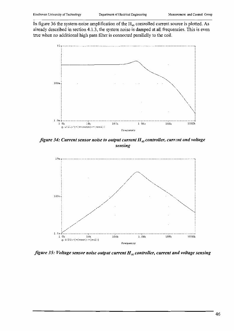
Eindhoven University of Technology Department of Electrical Engineering Measurement and Control Group
In figure 36 the system-noise amplification of the Hoo controlled current source is plotted. Asalready described in section 4.1.3, the system noise is damped at all frequencies. This is eventrue when no additional high pass filter is connected parallelly to the coil.
10 T ------------------------------------------------------------------------------------,
,,,100", J
IIIII I
1.Om+----------------r----------------T----------------,----------------,----------------41 Oh 10" 10Gh 1 OKh 10K" 100Kh
o 1(11)/(v(YsQurce)-v(vrul))
figure 34: Current sensor noise to output current H 00 controller, curr.mt and voltagesensing
lOmT------------------------------------------------------------------------------------,
Frequency
figure 35: Voltage sensor noise output current H 00 controller, current and voltage sensing
46

Eindhoven University of Technology Department of Electrical Engineering Measurement and Control Group
1.0 T ------------------------------------------------------------------------------------1, I, I
i -~--~i, I, I, II II II •I I, I, ,, ,, ,, ,, II II ,I •
1(;!!i.~ :
I ',,,,,,,,,,IIIII
~---_.
,,I ,
lGOu+---------------- r ---------------- T ----------------~----------------~----------------11 Oh 10h 100h 1.01(h 10Eh 100Kh
o V(Vout) /(II(Vgate)-V(Rl'J.2) )
figure 36: System noise amplification output voltage H 00 controller, current and voltagesensing
4.1.5 CONCLUSIONS REGARDING CURRENT SOURCES
In the previous sections the voltage controlled current source was examined as the actuator inthe magnetic levitation system. It appeared that it is very difficult to stabilise a current sourceloaded with coil, and that the output voltage of the current sources suffers from a lot of noise.This will lead to problems with the inductance measurement.
For these reasons the voltage controlled voltage source is examined as the actuator for themagnetic levitation system in the next section.
14.2 LINEAR VOLTAGE SOURCE
The power supply described in the section 4.1, was a voltage controlled current source(VCCS). It appeared that a current source is likely to oscillate when loaded with an inductor.An other possibility to drive the coil is to use a voltage controlled voltage source (VCVS)This option is examined in this section.The drawback of this option is that the magnetic reluctance force exerted on the ball by thecoil does not depend directly on the applied control voltage on the power supply. The extratransfer function of the actuator is introduced into the system, by the serial-connection of thecoil with its internal resistance. (See ( 24)) To make it even worse, this transfer function is notconstant, but depends on the distance between the ball and the coil. (See chapter 3.)One can say that noise and stability-problems are moved from the power supply to thecontroller of the levitation system.
47

Eindhoven University ofTechnology Department of Electrical Engineering Measurement and Control Group
For the target of the thesis is self sensing magnetic levitation, an other restriction of the powersupply is that the inductance of the coil can be measured simultaneously. Like with the currentsource, this is done by adding an extra high frequent voltage on top of the DC-voltage overthe coil. The frequency of this extra component must be much higher than the highestfrequency of the mechanical system. To add an additional signal around 1 kHz would be agood choice.
A voltage controlled voltage source can be realised as in figure 37. The extra voltageamplification by transistor T2 is necessary because the supply voltage of the circuit is morethan the supply voltage of the opamp. Diode D j and zenerdiode Zj have no function in thecircuit and are only for protection of the MOSFET Tj •
Vin
R2
Vout
D1
figure 37: Voltage Controlled Voltage Source
The output voltage Vout of the voltage controlled voltage source in figure 37 for lowfrequencies is given by: (When the gain ofthe opamp is assumed to be infinite.)
(32)
The VCVS must have a low-pass characteristic for stability, however the bandwidth of thevoltage controlled voltage source can be very high, in comparison with the voltage controlledcurrent source. The 3dB point is given by:
R[ +RzhdB = 2;rR
1R
2C
1
(33)
In contrast to the current source, there are no stability or noise problems when using a voltagesource.Note that care must be taken, when designing the controller for the whole levitation system,that the actuator does not saturate at its supply voltage.
48
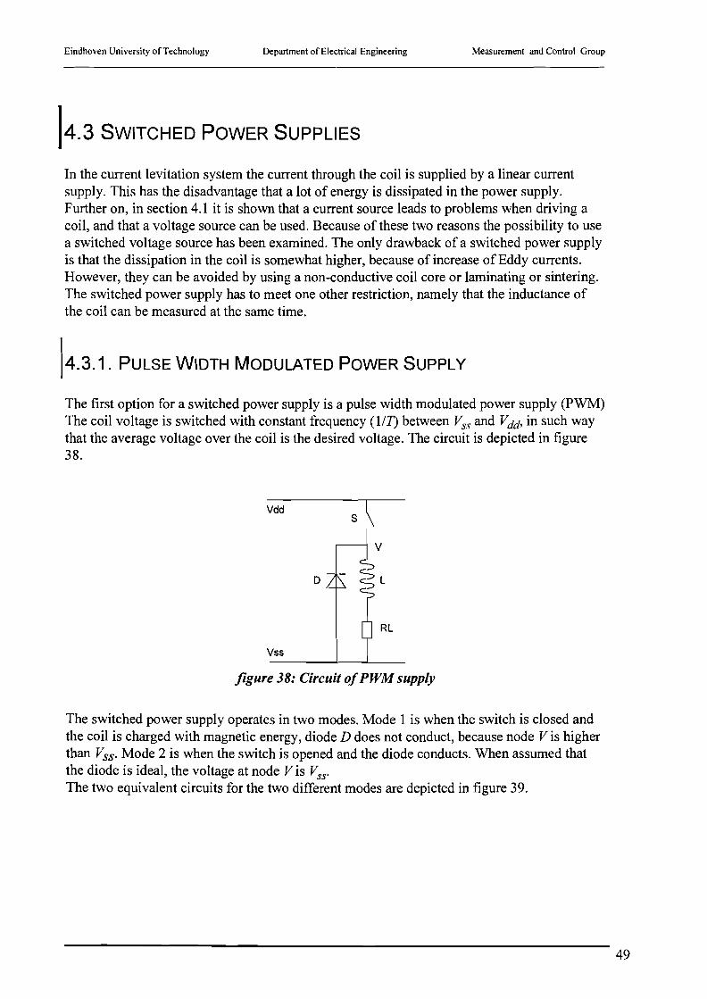
Eindhoven University of Technology Department of Electrical Engineering Measurement and Control Group
14.3 SWITCHED POWER SUPPLIES
In the current levitation system the current through the coil is supplied by a linear currentsupply. This has the disadvantage that a lot of energy is dissipated in the power supply.Further on, in section 4.1 it is shown that a current source leads to problems when driving acoil, and that a voltage source can be used. Because of these two reasons the possibility to usea switched voltage source has been examined. The only drawback of a switched power supplyis that the dissipation in the coil is somewhat higher, because of increase of Eddy currents.However, they can be avoided by using a non-conductive coil core or laminating or sintering.The switched power supply has to meet one other restriction, namely that the inductance ofthe coil can be measured at the same time.
4.3.1. PULSE WIDTH MODULATED POWER SUPPLY
The first option for a switched power supply is a pulse width modulated power supply (PWM)The coil voltage is switched with constant frequency (1/1) between Vss and Vdd' in such waythat the average voltage over the coil is the desired voltage. The circuit is depicted in figure38.
Vdd
D
Vss
figure 38: Circuit ofPWM supply
The switched power supply operates in two modes. Mode 1 is when the switch is closed andthe coil is charged with magnetic energy, diode D does not conduct, because node V is higherthan Vss. Mode 2 is when the switch is opened and the diode conducts. When assumed thatthe diode is ideal, the voltage at node V is Vss'
The two equivalent circuits for the two different modes are depicted in figure 39.
49

Eindhoven University of Technology Department of Electrical Engineering Measurement and Control Group
Vd
Mode 1 Mode 2
figure 39: Equivalent circuits for PWMpower supply
The average current through the coil iL,av can be calculated as follows:
J _ c5. Vdt!...L,av - R
L
( 34)
where c5 is the duty cycle ofthe steering ofthe switch.A high frequency saw-tooth wave form is superposed onto this average current through thecoil by the switching of the power supply. The amplitude of this saw-tooth is a measurementfor the inductance ofthe coil. The amplitude of the saw-tooth can be calculated as follows:(See also figure 40)
( 35)
RWhen assumed that T «-{ :
50
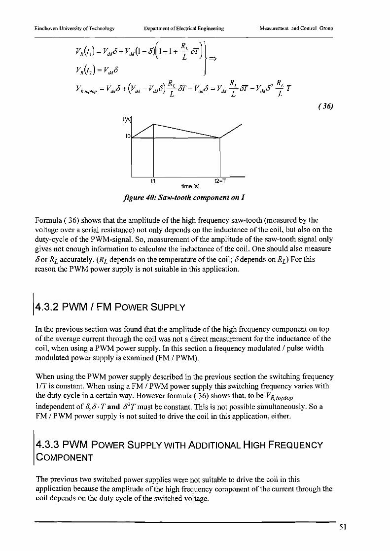
Eindhoven University of Technology Department of Electrical Engineering Measurement and Control Group
I[A
10iL-_-+- ----:::::::-'('
(36)
t1 t2=Ttime [5]
figure 40: Saw-tooth component on I
Formula (36) shows that the amplitude of the high frequency saw-tooth (measured by thevoltage over a serial resistance) not only depends on the inductance of the coil, but also on theduty-cycle of the PWM-signal. So, measurement of the amplitude of the saw-tooth signal onlygives not enough information to calculate the inductance of the coil. One should also measure
t5 or RL accurately. (RL depends on the temperature of the coil; 8 depends on RL) For thisreason the PWM power supply is not suitable in this application.
4.3.2 PWM I FM POWER SUPPLY
In the previous section was found that the amplitude of the high frequency component on topof the average current through the coil was not a direct measurement for the inductance of thecoil, when using a PWM power supply. In this section a frequency modulated I pulse widthmodulated power supply is examined (FM I PWM).
When using the PWM power supply described in the previous section the switching frequencyIff is constant. When using a FM I PWM power supply this switching frequency varies withthe duty cycle in a certain way. However formula (36) shows that, to be VR,toptop
independent of 8, 8 .T and 8 2T must be constant. This is not possible simultaneously. So aFM I PWM power supply is not suited to drive the coil in this application, either.
4.3.3 PWM POWER SUPPLY WITH ADDITIONAL HIGH FREQUENCY
COMPONENT
The previous two switched power supplies were not suitable to drive the coil in thisapplication because the amplitude of the high frequency component of the current through thecoil depends on the duty cycle of the switched voltage.
51

Eindhoven University of Technology Department of Electrical Engineering Measurement and Control Group
For that reason, a switched power supply with two switching frequencies is examined. Thefirst frequency is pulse width modulated to control the current through the coil, the second hasa even higher frequency and a constant duty cycle of 50%. It is examined whether the currentthrough the coil at the highest frequency does not depend on the duty-cycle of the lowestfrequency.
There are three different ways to combine two frequencies in a switched current supply. Theyare all Boolean functions. All three ways have a different effect on the duty cycle of theresulting signal. (See table 3.)
function result duty cycleAND always < 50%OR always> 50%XOR always = 50%
table 3:Functions to combine two frequencies in switchedpower supply
The XOR-gate can not be used in a switched power supply, because the duty cycle is always50%, and thus the output power ofthe supply can not be controlled. Only the AND-function issuitable to be used in the switched power supply for this application, because the controllermust be able to reduce the output power of the supply to nearly zero.When the AND-function is used in the PWM supply as depicted in figure 38, the voltage overthe coil, will be that as in figure 41, the current through the coil will be that as in figure 42<
VL[
time [s]
figure 41: Voltage over the coil in PWM supply with additional high frequency component
parallel lines
time [s]
figure 42: Current through the coil in PWM supply with additional high frequencycomponent
When assumed that T« i- the current through the coil (measured by a serial resistance) can
be calculated as follows:
52

Eindhoven University of Technology Department of Electrical Engineering Measurement and Control Group
(37)
The top-top value of the high frequency component in that current (voltage over the serialresistance) is:
V (C) 1 V 5+ RL 5(l-5)T+(l-5)+!(l-5) RL TVn,HF,/op/oP = VR(A) - VR(B) + :n. .2/ = ;d. L (1- 5)jT 2 L
(38)
Formula ( 38) shows that, although the duty cycle ofthe high frequency component blockwave is constant at 50%, the amplitude of the saw tooth still depends on the duty cycle of thelow frequency PWM signal.Physical explanation for this phenomenon is the serial resistance of the coil. When the switchis closed, the voltage over the coil is Vdd(l- 5) and not Vdd. When the switch is opened the
voltage over the coil is Vdd5 and not zero. Thus the amplitude ofthe high frequency voltage
over the coil depends on the duty cycle 5 and so does the amplitude of the current.This is true for all basic switched power supplies. So the amplitude of the high frequencycurrent through the coil is not a good measurement for the inductance of the coil. For thatreason in the next section, a switched power supply is proposed where the switchingfrequency of the supply is a measure for the inductance of the coil.
4.3.4 SERIAL RESONANT SWITCHED POWER SUPPLY
In the previous sections the amplitude of certain signals was a measurement for the inductanceof the coil. It appeared that this was not easy to implement. In a resonant switched powersupply not the amplitude, but the frequency of the current through the coil is measured. Thecircuit of a serial resonant switched power supply is depicted in figure 43.
53

Eindhoven University of Technology Department of Electrical Engineering Measurement and Control Group
+
Vdd
D1 81
c L RL
+
Vdd
D2
Vr---t---l ~J'J'J'-CJ--I
82
figure 43: Circuit 0/serial resonant switchedpower supply
The switches 8] and 82 conduct alternatively, with a certain duty cycle. So the voltage at nodeV is (in this sequence): +Vddwhen 8] is closed (82 opened, D] and D2 do not conduct), -Vddwhen D2 conducts (8] and 82 opened, D] does not conduct), -Vddwhen 82 is closed (8]opened, D] and D2 do not conduct) and +Vddwhen D] conducts (8] and 82 opened, D2 doesnot conduct).When the sequence as described above, is repeated at the resonance frequency of the serial LCcircuit, the current through the inductor can be controlled by the duty cycle of the 8] and 82.
The current through the inductor is given by the well known equation:
( 39)
The resonance frequency of the RL, L and C in serial is (when RL «2# ):
1fo =2ITHe
( 40)
So the output power of the resonant power supply is controllable, given by ( 39), and theinductance is observable, given by ( 40).
However, there is one problem: The impedance of coil is 2ifoL , so when roughly estimatedvalues for/o and L are used, the impedance of the coil is:
J 2
Z = ~(2;ifoL) ~ 2·IT ·1000· 0.1 ~ 6300
( 41)
A current of approximately 2A is needed to levitate the ball. So, the voltage over the coil withthat current will be:
V =z· iL ~ 630·2 =1260V
(42)
54

Eindhoven University of Technology Department of Electrical Engineering Measurement and Control Group
This voltage is much too high for safe operation, and much to high for normal capacitors. It isnot possible to force a DC-current through the coil, because of the serial capacitor. So a serialresonant switched power supply is not suited to be used in this application.
4.3.5 PARALLEL RESONANT SWITCHED POWER SUPPLY
In the previous section a resonant power supply with a capacitor in serie with the inductancewas examined. In this section a parallel switched power supply will be discussed. This has theadvantage that a DC-current can flow through the coil.The circuit of a parallel resonant switched power supply is given in figure 44.
Vdd
~ C
v
~LC;
_~RLfigure 44: Circuit ofparallel resonant switched power supply
The circuit in figure 44 is nearly the same as in figure 38 except that the diode is replaced by acapacitor. When the switch is closed, a current starts to flow through the switch into the coil.When the switch is opened, that current continues to flow through the coil, so it is drawn fromthe capacitor. The capacitor charges, the inductor discharges. This process continues until theinductor is completely discharged and the capacitor is fully charged. At this point, the currentis zero, and the voltage at node V has reached its minimum. Then the current starts to flow inthe other direction. The capacitor is discharged and the inductor charges, however, the currentis flowing in the other direction now. When the voltage over the capacitor is zero the inductoris fully charged. The current continues to flow in the other direction, until all energy in theinductor is in the capacitor again. The voltage at node V is at its maximum now. The currentswitches direction again, and the capacitor is discharged, until the voltage at node V is Vdd.Then the switch is closed again. (See figure 45)
The current through the coil can be controlled by the duty cycle of the switch. The current isgiven by (39). The inductance of the coil can be measured by the resonance frequency oftheLC-circuit. The resonance frequency is given by ( 40).
55

Eindhoven University of Technology Department of Electrical Engineering Measurement and Control Group
I[A]
v [V]
1 closed81 close 81 openedtirne[s]
figure 45: Signals in parallel resonant switched power supply
However, there is one problem with this parallel resonant switched power supply, viz. that theenergy stored in the coil must be stored in the capacitor completely. The energy in theinductor and capacitor is:
1 .2El = - Lll, 2 '
1 2E(. = -CUe'
- 2
( 43)
When roughly estimated values forfo, Land iL are used, the voltage over the maximumvoltage over the capacitor will be:
(44)
This voltage is much too high for safe operation.
It is not possible to enlarge the capacitor because then the resonance frequency would not bemuch higher than the bandwidth of the mechanical system. This would lead to high frequencymovements of the ball, and therefore wrong measurement of the position.So a parallel resonant switched power supply is not suitable as a power supply in thisapplication.
56

Eindhoven University of Technology Department of Electrical Engineering Measurement and Control Group
14.4 CONCLUSIONS REGARDING THE ACTUATOR
In this chapter various actuator types were examined for the magnetic levitation system. Insection 4.1 the current source was described. It appeared that a current source loaded with acoil is very likely to oscillate, and that the output voltage of the current source suffers fromexcessive noise. Therefore two Hoo controllers were designed for stabilising the currentsource. The first Hoo controller only observes the current through the coil, the other controllerobservers the current as well as the voltage over the coil. Although the latter performs betterregarding to noise reduction, it cannot be used in combination with the inductancemeasurement schemes involving an LC oscillator.The other type of actuator for the magnetic levitation system is the voltage controlled voltagesource, described in section 4.2. It appeared that the voltage source (loaded with a coil) doesnot have any of the disadvantages of the current source.Finally switched power supplies were examined as the actuator for the magnetic levitationsystem. It was shown that it was not possible to simultaneously use the coil as actuator andposition sensor when using a switched power supply.
Regarding above, one can see that the voltage controlled voltage source is the best actuatortype for the levitation system. However, as will be shown in the next chapter, it is verydifficult to combine the voltage source with any sensor.
57

Eindhoven University of Technology
5. SENSORS
Department of Electrical Engineering Measurement and Control Group
Keypoint of this thesis is (quasi) self sensing magnetic levitation. That means that the positionof the levitated ball is not measured by an additional position sensor (such as a camera) but bymeasuring the inductance of the same coil that levitates the ball. This rises one big problem,namely how to measure the inductance of the coil, at the same time a control current is forcedthrough it.An other problem is that the coil suffers from saturation and hysterese by the control current.(See chapter 2.) This influences the measurement of the inductance, and will lead to errors inthe position sensing.Several options for the sensor are examined throughout this chapter. In the next chapter achoice is made for a particular actuator/sensor combination.
The most simple way to measure the inductance of the coil, at the same time the controlcurrent flows through it, is by alternating between the two operating modi (control andsensing) at a high frequency. The sample theorem ofNyquist requires that the frequency atwhich the position of the ball is measured, is at least twice the maximum frequency in thesystem. In [10], [11] and [12] the maximum frequency of the mechanical system is assumed tobe 100Hz. This means that the sample frequency is at least 200Hz, but that 1kHz would besensible, because of the phase shift due to sampling.The time slot in which the coil is used as sensor can not be very long, in comparison to thetime the coil is used as an actuator, because the average current through, or voltage over thecoil is given by the output of the controller. Assume that for 10% of the time, the coil is usedfor sensing the position, and for 90% of the time the coil is used as actuator. (That means that
the duty cycle <5is 0.1)1
This gives a time of about f' <5 =1· 10-3 ·0.1 ::: 1.10-4 [s] in which the measurement has to
take place. However, the time constant ~ is about ~:= 0.1 ::: 3 .10-2 [s]. So the currentRL RL 3.5
flowing through the coil during the actuating modus, will continue to flow through the coilduring the sensing modus. The sensor must allow this current to flow, or else the voltage overthe coil will rise to very hi,gh potentials. An other effect of the continuous current through thecoil is that unwanted effects, such as saturation, (still) influence the measurement.
Increasing the serial resistance of the coil, to reduce the time constant ~L is not a solution,
because then the voltage ever that resistance VR ::: IL • RL would be very large: When the timeconstant is reduced by (only) a factor 1000, the voltage over the resistor would be enlarged bya factor 1000. That voltage would then be a few kVolt.
The above leads to the conclusion that alternating between actuating and sensing with the coilis in the practical application not possible. All proposed sensors are therefore continuous.
An other point ofattention is that the serial resistance of the coil to be measured is not aconstant but temperature dependent. Its value is in the range:
58

Eindhoven University of Technology Department of Electrical Engineering
RL min =2.50 RL nom =3.50 RL max =4.50, , ,
Measurement and Control Group
( 45)
In the next sections various way to measure the inductance of the coil are proposed. First,three different ways to obtain the inductance of the coil involving an LC-oscillator areexamined: In section 5.1. the oscillation frequency of the LC-oscillator is measured using aphase locked loop. In section 5.2 the oscillation frequency of the LC-oscillator is measured bycounting pulses between two zero crossings. And finally in section 5.3 the quality factor ofthe LC-oscillator is examined.In section 5.4 an additional high frequency component is added to the voltage over the coiland the high frequency current is measured, to obtain the inductance. Also the dual case (add ahigh frequency current and measure high frequency voltage) is examined.In section 5.5 correlation measurement is examined as a way to obtain the inductance of thecoil.For all these different ways to measure the inductance of the coil, constraints to the circuit, theinfluence of the actuator on the sensor, the influence of the sensor on the actuator and thesignal to noise ratio of the measurement is determined.
15.1 MEASURING LC-OSCILLATION FREQUENCY WITH PLL
One way to measure the inductance of a coil is to measure its oscillation frequency incombination with a (known) capacitor. The oscillation frequency of a LC-oscillator (when itsdamping is small) is given in ( 40). However, the actuating current must be supplied to thecoil also. This gives the circuit as in figure 46.
Power Amplifier
figure 46: LC-Oscillator sensor
Chapter 4 showed that the power amplifier can either be a voltage source or a current source.First the consequences of using a voltage source are examined. After that the current source isdiscussed.One possibility to determine the inductance of the coil is to measure the oscillation frequencyof the LC-oscillator with aphase locked loop (PLL). This is examined in section 5.1.3. Another way to measure the oscillation frequency is counting pulses between two zero-crossings(examined in section 5.2) The inductance of the coil can also be obtained by determining theQ-factor of the LC-oscillator (examined in section 5.3)
59

Eindhoven University ofTechnology Department of Electrical Engineering Measurement and Control Group
5.1.1 LC-OSCILLATOR WITH VOLTAGE SOURCE
The output impedance of an ideal voltage source is zero, so the LC-oscillation of the oscillatorin figure 46 would be totally damped. A solution for this contradiction is to increase theoutput impedance of the voltage source around the oscillation frequency of the LC-oscillator.(The power amplifier is then converted to a current source, at that frequency) This can bedone by an external LC-filter. (See figure 47.)
Lf
Rf
figure 47: LC-Oscillator sensor, with LC-filter
Note that the LC-oscillator in figure 46 (and figure 47 too) is a parallel LC-oscillator. Aparallel LC-oscillator can be connected to a current source. The dual case, a serial LCoscillator, can be connected to a voltage source. However when a capacitor is in serie with thecoil, no (actuating) DC-current can be forced through the coil.
It is desired that the oscillation frequency of the oscillator only depends on the inductance ofthe coil. Therefore the influence of the various components in figure 47 is examined. They areexamined separately, to avoid mathematical complexities.
Influence of RL
In figure 48 the equivalent schematic of figure 47 is plotted, when the influences of Lf CfandRfon the oscillation frequency are neglected.
L
RL
c
figure 48: Equivalent scheme/or calculating influence 0/R[
The impedance of the schematic in figure 48 is given by:
I'mC(jmL + RL )
Z(jm) = ) -1 1 1- m2LC + j mR C--+--+R L
jmC jmL L
( 46)
60

Eindhoven University of Technology Department of Electrical Engineering Measurement and Control Group
When ~I «4 L~' which is true in this application (1 «130000), ( 46) can be approximated
by:
. 1 RL- jf1J---
Z(Jm)~ C LC
( m+ RL +j rI)(m+ RL _ j rI)2L ~LC 2L ~LC
( 47)
Formula ( 47) shows that RL has 'no' influence on the oscillation frequency, when
R2 1L~'- « 4 LC . This influence decreases with increasing foZ.c·
Influence of Rf
In figure 49 the equivalent schematic of figure 47 is plotted, when the influences ofLfi CfandRL on the oscillation frequency are neglected.
figure 49: Equivalent schemefor calculating influence ofRf
The impedance of the schematic in figure 49 is given by:
(48)
When Rf » JL , which can be true (Rf»628), ( 48) can be approximated by:vC
1-jm-
Z(Jm)~ C
(m+_1
+j rIJ(m+-1j rIJ2R
fC ~ LC 2R
fC - ~LC
( 49)
Formula ( 47) shows that Rf has 'no' influence on the oscillation frequency, when
ifRf » ,) C . This influence increases with increasing ~losc .
61

Eindhoven University ofTechnology Department of Electrical Engineering Measurement and Control Group
In this approximation Rfis not only Rfof figure 47, but can also be the output impedance of atrue current source as described in chapter 4, or the characteristic impedance of the LC-filterin figure 47.
Influence of Cf and Lf
In figure 50 the equivalent schematic of figure 47 is plotted, when the influence of RL on theoscillation frequency is neglected.
R
figure 50: Equivalent scheme/or calculating influence 0/Lfand Cf
For the equivalent scheme of figure 50 the following relations apply:
• L·LfL =--L+Lf
C· = C + Cf
(50)
The optimum case is when Lfequals L and Cfequals C. When this is the case L* is decreasedby a factor 2 and c* is increased a factor 2. So the oscillation frequency is still
1lose = 2;rrJLC .
However, in the previous paragraph it derived that to have no influence on the oscillation
frequency Rf »~~ . The characteristic impedance ofthe parallel connection of Lfand Cf is:
Z = ILf. So the parallel connection of Rfand Lfand Cfhas an impedance which is always
VCf
smaller than #.This means that the filter in serie with the voltage source always influences the oscillationfrequency of the LC-oscillator. In other words, when a voltage source is used as the actuatorofthe levitation system, and the induction sensor involves an LC-oscillator, the influence ofthe filter on the inductance measurement must be compensated for.
5.1.2 LC-OSCILLATOR WITH CURRENT SOURCE
In section 5.1.1 the power amplifier of figure 46 coil was a voltage source. In this section acurrent source is used as a power amplifier. However, it was made clear in the previous
62

Eindhoven University ofTechnology Department of Electrical Engineering Measurement and Control Group
chapter that the coil voltage suffers from a lot of noise when using a current source. Anadditional high-pass RC-filter is needed to limit the impedance of the load at high frequencies.The influence of this filter on the oscillation frequency of the oscillator is examined in thissection.Note that the output impedance of the current source and the serial resistance of the coil RLalso influence the oscillation frequency. The influence of the output impedance of the currentsource is comparable to the influence of Rf . The influence of Rfand RL is already examined inthe previous section.
When the additional high-pass filter is added to the circuit of figure 46, this leads to aequivalent circuitry as depicted in figure 51.
L
R
figure 51: LC-oscillator with current source
The impedance of the circuit in figure 51 is given by:
1z= 1 I
j roC + 1 + J'~m->L-+-R-L--+R
• ~_J""' fJW\.-f
=
=- jm3LCCfRf - m2(LC + CCfRfRL+ LCf ) + jW(RLC + RLCf + RfCf ) + 1
( 51)
When Cf-<C and Rj»RL this can be approximated by:
(52)
Formula ( 52) is true only when Cf-<C and Rj»Rr. this means that Cfand Rfmust be:
63

Eindhoven University of Technology Department of Electrical Engineering
{C~200nF
Cf «200nF~ Cf < 200pF
{RL ~ 3.50
Rf »3.50~ Rf > 3KO
Measurement and Control Group
(53)
When Rf and Cf satisfy ( 53) no compensation is necessary in the measurement for the(known) influence ofRfand Cf
5.1.3 MEASURING FREQUENCY WITH A PLL
The oscillation frequency of the oscillator in figure 46 can be measured by using a phaselocked loop. (See figure 52.) However, because of the additional, unavoidable noise at theinput of the phase detector of the PLL (for example due to the low frequent actuating currentthrough the coil), the measurement of the frequency of the oscillator suffers from noise.
Vin inputfilter
phasedetector
loopfilter
voltagecontrolled f---'-----7oscillator
figure 52: Phase Locked Loop
In [14] the behaviour of a PLL with a noisy input signal is examined. The noise signal isassumed to have a flat spectrum in a small frequency band around the oscillation frequency ofthe oscillator OJi' (Because of the input filter of the phase detector.) In that case the noisesignal n(t) can be written as:
n{t) =r{t) cos( Ill;! + lpi{t))
r{t),lpi{t) = stochastic
(54)
The noise signal C.ln be decomposed in quadrature components:
(55)
The two input signals of the phase detector of the PLL can be written as:
v;/t) = ~(t) + n{t) = r;,l .sin(OJ;! + B;{t)) + nJt) cos(OJ;!) + n.,{t) sin(OJ;!)
V;.2{t) =v,'cJt) = 110 . cos(OJ;! + e,,{t) + o"Jt))
(56)
64

Eindhoven University of Technology Department of Electrical Engineering Measurement and Control Group
where Bo(t) is the phase shift necessary to lock the PLL, Bno(t) is the output noise of the PLL,Vs{t) is the output signal of the input filter without additional noise and Vvco(t) is the outputvoltage of the voltage controlled oscillator (YeO). When assumed that the phase detector isan ideal multiplier with a small gain Kd, and that the signal to noise ratio of the input signal ofthe phase detector is relatively high (>4dB), the output voltage Vd0fthe phase detector isgiven by:
(57)
Because the loop filter is linear and the voltage controlled oscillator can be considered to havea linear transfer function from input voltage to output frequency, the signal to noise ratio ofthe output of the PLL {SNR)out can be calculated by multiplying Vdwith the transfer functionof the filter and Yeo. This gives:
(SNRLul =(SNR) i/l • 2~ ,L
(58)
where Bi is the bandwidth of the input filter of the PLL and BL is the noise bandwidth of theloop filter of the PLL. For a second order loop filter with a normalised transfer function as in (59) this noise bandwidth BL is given in ( 60).
(59)
(60)
For different loops this relation reduces to:
high gain: a == 0: BL =
The bandwidth of the loop filter determines how fast the PLL is, the noise bandwidth of theloop filter determines (in combination with the input filter of the PLL) the phase jitter. Theratio between the two is therefore interesting. (See also figure 53)
65
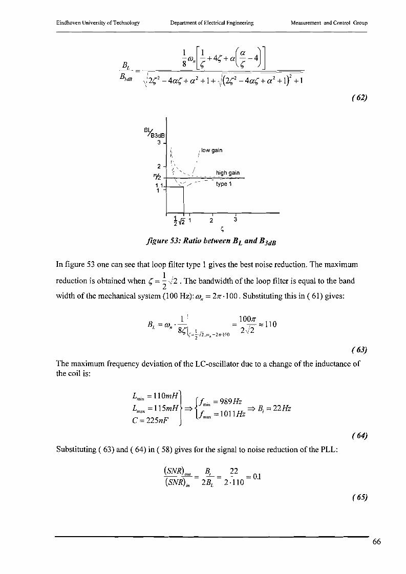
Eindhoven University of Technology Department of Electrical Engineering Measurement and Control Group
\
~\ floW gain
r\2 11',_ /
\ - high gain'Y2 +--.;-------'-~~~--\'-/' - t 11.1+-_'.:.., ./ ype
1
(62)
I
~ v'2 1 2 3
~
figure 53: Ratio between BL and B3dB
In figure 53 one can see that loop filter type 1 gives the best noise reduction. The maximum
reduction is obtained when C; =~ J2 .The bandwidth of the loop filter is equal to the band
width of the mechanical system (l00 Hz): 0)" =21r·l 00. Substituting this in ( 61) gives:
1 iB =0) •-I = 1O~ ~ 110
L "8/'1 I 2-v2'=' l,r~--fi OJ =211"·\00, 2 • n
(63)
The maximum frequency deviation of the LC-oscillator due to a change of the inductance ofthe coil is:
Lmin =110mH} {f.. =9 '9 u:mm 8 nZ
Lmax =115mH => f. = 1011Hz => Bj = 22HzC =225nF max
(64)
Substituting ( 63) and ( 64) in ( 58) gives for the signal to noise reduction of the PLL:
(65)
66

Eindhoven University of Technology Department of Electrical Engineering Measurement and Control Group
Substituting ( 65) shows that the PLL amplifies(!) the noise at the input to the output by afactor 10. Physical explanation for this phenomenon is that the PLL must get all its information out of a maximum frequency sweep of 22 Hz, and that this sweep can take placewith a maximum frequency of 100 Hz. It is easy to understand that such a measurementcomes with a lot of noise.
5.2 MEASURING LC-OSCILLATION FREQUENCY WITH HFCOUNTER
In section 5.1 the oscillation frequency of the LC-oscillator was measured using a PLL. Another way to measure a frequency is to count the number of pulses of (known) HF-sourcebetween two zero crossings of the LC-oscillator output. This gives a system which is alreadydepicted in figure 46. The influences of various filters necessary to drive the coil are alreadyexamined in the previous section. Therefore in this section only a relation between the signalto noise ratio of the output of counter and the signal to noise ratio of the input is derived.
In figure 54 the input signal of the comparator is depicted. The comparator has hysteresis, toavoid high frequency noise at the output of the comparator at the switching point. The twodetection levels of the comparator are also depicted in figure 54.
Voltage[V],--------.
output hysteresecomperator
time[s]
figure 54: Input signal ofthe hysterese-comparator
In figure 55 an enlargement of the region inside the circle of figure 54 is depicted.
t" ~ - - ttrue
figure 55: Enlargement ofnoisy signal around Vhys
67

Eindhoven University of Technology Department of Electrical Engineering Measurement and Control Group
Because a very small band pass filter around the oscillation frequency of the LC-oscillator ())s
leads the comparator, to filter as much noise as possible, the noise Vn(t) can be assumed to
have very small band pass characteristic around ())s (which is not the case in figure 55), thenoise can be approximated by:
v" (t) =Vn.sin(OJ,J + On) ,(66)
where On is stochastic and 9;, is the maximum amplitude of the noise signal. (*Maximumamplitude ofthe noise: See later on.) The noisy signal Vs(t)+ Vn(t) can be written as:
..,. () ..,. ( ) ! ..,.2 ..,...,. (). [ ( 9;, sin(0,,) )Jv, t + vn t =1)1 + v, + 2v,vn cos 0" .sm OJ.! + arctan..,. ..,. ()vs + V n cos 0"
(67)
The maximum phase error of the comparator due to the additional noise can be calculated asfollows:
[( P;, sin(0,,) l]d arctan,
__ \. r, + rn cos(o,J = 9;, (~, cos(On) + 9;,) =0
d 8" 29;,p., cos(0,,) + 9;,2 + p"2
~ cos(0,,) = - ~'s
( 9;,)~ 0" =arccos - JI,.
(68)
When the result of ( 68) is substituted in ( 67), this gives for the maximum phase error of thecomparator:
B"rror,max =arctan
f. sinlarccos(-1.)Jf, +~ cos(arccos(- ~JJ
(69)
According to the definition in ( 72) the signal to noise ratio of the output is:
(70)
68
Eindhoven University of Technology Department of Electrical Engineering Measurement and Control Group
Formula ( 70) shows that the signal to noise ratio at the output has a minimum (worst) value.This arises from the assumption that the noise has a very small band pass characteristic, andhas a certain maximum value.
For small values ofx arcsin(x) ~ x. This reduces (70) to:
(SNRLut = 1(SNR);11
(71)
Remark that the result of formula ( 71) compared to the result of formula ( 65) seems to besomewhat optimistic. For in both cases the frequency of an oscillator is used as a measure forthe inductance of the coil. Probably, the signal to noise ratio of the sensor described in thissection is much less than formula (71) shows.
(*) Note that in this section for simplicity the signal to noise ratio is not defined as the powerof the signal divided by the power of the noise, but as the maximum amplitude of the signaldivided by the maximum amplitude of the noise.
(SNR) JI, IIVsII.,(Jut = r = 'IVII
fl I" iXI
(72)
This means that not all noise-models can be used in this approximation. For exampleGaussian noise can not be used, because the 'amplitude' of Gaussian noise goes to infinity:
(73)
wheref.xfx) is the probability density function.
15.3 MEASURING LC-OSCILLATOR Q-FACTOR
In the previous sections the oscillation frequency of the LC-oscillator was measured. In thissection the Q-factor of the oscillator in figure 47 is measured as a sensor for the inductance ofthe coil. The impedance of a circuit as given in figure 56 is:
69

Eindhoven University of Technology Department of Electrical Engineering Measurement and Control Group
(74)
Rf c
figure 56: Equivalent schematic/or Q-factor measurement
This can be written as:
(75)
As can be seen in ( 75), Qp does not only depend on L, but also on Rr- (To be more precisely,
Qp oc )i ,Qp oc ~ -) So, to measure L from the quality factor Qp of the oscillator, Rr must beL
measured too. (Rr is temperature dependent.) For this reason Q-factor measurement is not agood method for measuring the inductance of the coil, in this application.
5.4 MEASURING ADDITIONAL HIGH FREQUENCY
COMPONENT
An other option for measuring the coil inductance which will be examined in this report, isadding an extra high frequency component with a constant amplitude to the band limitedcontrol voltage over the coil or current through the coil. Because both a voltage source and acurrent source can be used to drive the coil, this option is examined first for voltage control,and after that for current control.
5.4.1 HIGH FREQUENCY COMPONENT WITH VOLTAGE CONTROL
When a high frequency component is added to the band limited control voltage over the coil,the extra high frequent current through the coil is a measurement for the inductance of thecoil:
70

Eindhoven University of Technology Department of Electrical Engineering
1i = ·UL R
L+ jmL L
Measurement and Control Group
(76)
Formula ( 76) shows that the current is not inversely proportional with the inductance,because of the serial resistance of the coil. There are two ways to overcome this problem.The first is to add a very high frequency, so that mL » RL • This will lead to certain (butsmall) error, depending on the measuring frequency. Problem is that a very high frequencyvoltage over the coil will lead to a very small current. Noise will disturb the measurement ofthis current.The second solution for the problem is not to measure the amplitude of the total current, but tomeasure the amplitude and phase of the high frequency current. This option will be discussedin this section.
A phase diagram of the voltage over the coil VL and its serial resistance VR, due to a currentthrough the coil h is depicted in figure 57. Vs is the voltage applied voltage over the serialconnection of the coil and the internal resistance. (See also figure 58.)
Vs
\VD
figure 57: Phase diagram ofcurrent and voltage over coil
From figure 57 the following two relations for the serial connection of the coil with itsresistance can be derived: .
(77)
Substituting the two formulas from ( 77) into each other gives:
(78)
71

Eindhoven University of Technology Department of Electrical Engineering
Voltage source
Measurement and Control Group
+ ! +VRs VR
- I - I
figure 58: Current sensing resistor circuitry
When the voltage over an extra serial resistance Rs with the coil (to measure the current iLthrough the coil, see figure 58) is multiplied with cos(mt) and after that is lead through a lowpass filter gives the DC-voltage: (This is also called synchronous AM-demodulation) [10],[11], [12]
Vdelll = [JlR, 0 sin(mt + ¢) + ~(lwJreq] 0 cos(mt) =
[JlR, • ( sin(mt) cos(¢) + cos(OJ() sin(¢))] . cos(mt) + ~owJreq 0 cos(mt) =1 1 low.pas."
'2 JlR•. sin(¢) + '2 JlR, sin(2mt + ¢) + ~owJreq cos(mt) =
~ JlR, sin(¢)
(79)
Substituting ( 79) and ( 77) in ( 78) leads to:
L=
Ii 0 _Vdem., 1
-JI2 R
JIR,-' omR,
( 80)
Formula ( 80) gives the equation which describes how the inductance (and so the position ofthe ball) can be measured with the DC-output voltage ofthe demodulator and the amplitude ofthe voltage over the extra serial resistance Rs. As the amplitude of the additional high
frequency voltage over the coil JI" its frequency m and Rs are constants, the relation betweenthe inductance of the coil L and the output voltage of the demodulator Vdem is proportional.Note that JlRs is not constant and must be measured separately.
Measurement of the voltage over the current sensing resistor comes with inevitable noise.This influences the accuracy of the inductance measurement of the coil. When assumed thatthe input voltage VRs suffers from band limited noise with frequency m, amplitude JI" and
stochastic phase B(See section 5.2) the input of the demodulator is given by:
72

Eindhoven University of Technology Department of Electrical Engineering
1\ . sin(mt + ¢) + }In' sin(mt + B)
Measurement and Control Group
( 81)
The output voltage of the demodulator is then given by:
Vdem = (}lR, . sin(mt + ¢) + JI" .sin(mt + B)). cos(mt) =
[}lR, (sin(mt) cos(¢) + cos(mt) sin(¢)) + JI" (sin(mt) cos(B) + cos(mt) sin(B))] cos(mt) =1 1 1 1 low.pass- }lR. sin(¢) + -}In sin(B) + -}lR sin(2mt + ¢) + -2}1n sin(2mt + B) =2' 2 2 ..
l}ln sin(¢) + l JI" sin(B)2' 2
(82)
The measured inductance is, according to ( 80), given by:
L _ 2RY,Vdem = Rs}l,(}lR, sin(¢)+ JI"sin(B))
- (}lR, + JI" sin(¢ - B)r(J) (}lR, + JI" sin(¢ - B)r(J)
(83)
Maximum of this function is reached when B= ¢. This maximum is:
R)~ sin(¢) . (}lR, + JI,,)Lmax = }I 2(J)
R.,
(84)
Using ( 80) and ( 84) gives for the signal to noise ratio(*) of the inductance measurement:
(SNRt'l -1(SNR). -
l/l
(85)
Formula ( 85) shows that the signal to noise ratio of the inductance measurement is equal tothe signal to noise ratio of the input signal of the sensor. (which is Rs)
(*) Again, in this section the signal to noise ratio is defined as the maximum amplitude of thesignal devided by the maximum amplitude of the noise. See section 5.2 for details.
73

Eindhoven University of Technology Department of Electrical Engineering Measurement and Control Group
5.4.2 HIGH FREQUENCY COMPONENT WITH CURRENT CONTROL
In the previous section a high frequent component is added to the voltage over the coil. Whena current source is used a high frequent component can be added to the current through thecoil. This has some advantages, as will be made clear in this section.The high frequency voltage over the coil is not a direct measurement for the inductance of thecoil, because of the serial resistance of the coil:
(86)
Like with voltage control, there are two ways to overcome this problem:The first is to add a very high frequency, so that wL » RL • This will lead to certain (butsmall) error, depending on the measuring frequency. Problem is that a very high frequencycurrents can not be supplied to the coil, due to the high impedance of the inductor at thatfrequency.The second solution for the problem is not to measure the amplitude of the total voltage, butto measure the amplitude of the voltage which is 90° out of phase with the applied current.This option will be discussed in this section.
A phase diagram of the voltage over the coil VL and its serial resistance VR, due to a currentthrough the coil iL is depicted in figure 59. Note that this is the same diagram as in figure 57,except for the fact that now iL is known, and Vs (not VL) can be measured.
Vs
VI::;
figure 59: Phase diagram ofcurrent and voltage over coil
The vector diagram in figure 59 shows that the voltage over the inductive part of the coilimpedance is always 90° out ofphase with the applied high frequency current. This has someadvantages:
When the voltage over the serial-connection of the coil inductance and resistance (Vs) ismultiplied with cos(wt) and after that is lead through a low pass filter this gives the DC~voltage:
74

Eindhoven University of Technology Department of Electrical Engineering Measurement and Control Group
Vdem = [17•.sin(m( + ¢) + ~ow.freq.] • COS(m() =
[~ . (sin(m() COS(¢) + COS(m() sin(¢))] . COS(m() + ~ow.freq • COS(m() =I I low. pass.
2~ sin(¢) + 2~ sin(2m( + ¢) + ~aw.freq cos(m() =
~ ~,sin(¢)
(87)
Substituting ( 87) in ( 78) leads to:
L = ~. sin(¢) = 2Vdem
iL • W iLm
( 88)
Formula ( 88) gives the equation which describes how the inductance (and so the position ofthe ball) can be measured with the DC-output voltage of the demodulator. Remark that the
amplitude of the applied high frequent current through the coil iL and its frequency mareconstants. This means that, in contrary to the voltage controlled coil, only the output voltageof the demodulator Vdem must be measured.
Like with the voltage controlled coil, the measurement of the coil voltage comes withinevitable noise. When assumed that the input voltage Vs suffers form band limited noise with
frequency m, amplitude r" and stochastic phase B(See section 5.2) the input of thedemodulator is given by:
17, .sin(m( + ¢) + r" .sin(m( + B)
(89)
The output voltage of the demodulator is then given by:
Vdem =(~ .sin(m( + ¢) + r" .sin(w( + B)). cos(m() =
[17. (sin(m() cos(¢) + cos(m() sin(¢)) + 17n(sin(m() cos(B) + cos(W() sin(B))]cos(m() =1 1 1 1 low.pass
2~. sin(¢) + 217n sin(B) + 217s sin(2m( + ¢) +2r" sin(2m( + B) =
~ 17, sin(¢) + ~ 17nsin(B)
(90)
The measured inductance is according to ( 88) given by:
75

Eindhoven University of Technology Department of Electrical Engineering
L = 2Vdem = 17ssin(¢) + JI" sin(e)
tLOJ tLOJ
Measurement and Control Group
Maximum of this function is reached when e=¢. This maximum is:
U~ing ( 88) and ( 92) gives for the signal to noise ratio(*) of the inductance measurement:
P. sin(¢)
(SNR) = L = [[OJ = 17. =(SNR).out Lmax-L (~.+JI,,)sin(¢)_p.sin(¢) JI" III
tLOJ tLOJ
-'-c--(S_lVR-,-:-,)o=-ut =1(SNRL,
(91)
(92)
(93)
Formula ( 93) shows that the signal to noise ratio)fthe inductance measurement is equal tothe signal to noise ratio of the input signal of the sensor, which is the voltage over the coil.
Also, the high frequent current through the coil suffers from noise. It is assumed that theamplitude of the current through the coil is given by:
(94)
where i" is stochastic.
Substituting ( 94) and ( 77) in ( 87) gives:
1~ 2 2 2 ( .. .. ) OJL 1(.. .. )Vdem =-2 RL + OJ L lL + 1/1 ~. 2 2 2 =-2 lL + 1/1 O1L
RL +m L
(95)
Using ( 88) leads to:
(96)
This gives for the signal to noise ratio(*):
76

Eindhoven University of Technology Department of Electrical Engineering
(SNR) = Lmeasured (SNR)- L L = ~measured - real
(SNR) 0111 -1(SNR);n -
Measurement and Control Group
(97)
Remark that for this sensor the voltage sensing current source, as described in section 4.1.3,can be used. That means that no additional filter is necessary to stabilise the current source.This has the advantage that no compensation is necessary for the influence of such a filter onthe inductance measurement.
(*) Again, in this section the signal to noise ratio is defined as the maximum amplitude ofthesignal devided by the maximum amplitude of the noise. See section 5.2 for details.
15.5 CORRELATION MEASUREMENT
In the previous sections the inductance of the coil is measured by adding a particular sensingsignal to the control current or voltage over the coil. Problem of all these options was thenoise at the output of the power amplifier. In this section this noise is used as sensing signal tomeasure the inductance of the coil. This can be done by correlation measurement.
The impedance of the serial connection of the inductance L and the resistance RL of the coil isgiven by:
(98)
This means that the spectrum of the noise in the current through the coil is given by:
(99)
And that the spectrum of the noise in the voltage over the coil is given by:
( 100)
So when the spectrum ofthe noise in the coil voltage and the spectrum ofthe noise in thecurrent through the coil can be measured, the impedance of the coil can be calculated by:
77

Eindhoven University of Technology Department of Electrical Engineering
Iz( 'OJ): = .cDllo;se",ollage(jOJ), } I "cD (. )
~ lloi.\'e,CUrrelll } OJ
Measurement and Control Group
( 101)
However, the inductance of the coil can not be calculated when only the impedance of theserial connection of the inductance and the resistance is known. So an other measurement isnecessary to determine RL. This can only be done by using one of the methods described inthe previous sections. This means that correlation measurement can not be used to determinethe impedance of the coil in this application.
15.6 CONCLUSIONS REGARDING THE SENSOR
In this chapter various sensors for the self sensing magnetic levitation system were examined.The sensor must be adapted to the actuator type (voltage source or current source), howeverthe actuator influences the sensor. This influence must be compensated for.First the sensor examined was to measure the oscillation frequency of an LC-oscillator with aphase locked loop. It appeared that this combination has a very bad signal to noise ratio(compared to other sensors) Therefore it will not be used in the levitation system.The second sensor which was examined, was the HF-pulse counting between two zerocrossings. Although the signal to noise ratio of this sensor seemed much better than theinductance sensor using the PLL, it was remarked that the calculations of the signal to noiseratio was probably much too optimistic. Therefore this way to measure the inductance of thecoil will not be used in the levitation system.Next, the Q-factor of an LC-oscillator was examined as a way to obtain the inductance of acoil. It was shown that the Q-factor not only depends on the inductance ofthe coil, but also onits serial resistance RL. As the serial resistance RL of the coil is temperature dependent, thistype of sensor cannot be used in this application.The fourth type of inductance sensor which was examined was adding a high frequency signalto the current through the coil or voltage over the coil. It appeared that, when a using currentcontrolled coil, this type of sensor is accurate and simple.Finally the last sensor discussed was correlation measurement. It was shown that when usingcorrelation measurement only, the inductance ofthe coil cannot be obtained. For this reasonthis inductance sensor is not used in the magnetic levitation system.
One can say that, from the sensor's point view, a current controlled coil with an additionalhigh frequency component is the best option for the actuator/sensor combination in thisapplication.
78
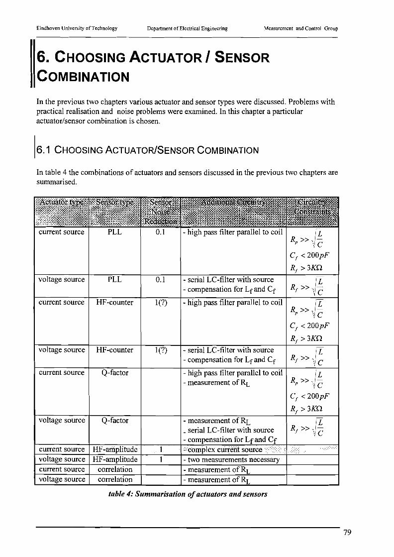
Eindhoven University of Technology Department of Electrical Engineering Measurement and Control Group
6. CHOOSING ACTUATOR I SENSOR
COMBINATION
In the previous two chapters various actuator and sensor types were discussed. Problems withpractical realisation and noise problems were examined. In this chapter a particularactuator/sensor combination is chosen.
6.1 CHOOSING ACTUATOR/SENSOR COMBINATION
In table 4 the combinations of actuators and sensors discussed in the previous two chapters aresummarised.
current source PLL 0.1 - high pass filter parallel to coilRp »{fCf < 200pF
Rf > 3Kn
voltage source PLL 0.1 - serial LC-filter with sourceRf »{f- compensation for Lf and Cf
current source HF-counter 1(7) - high pass filter parallel to coilR »{f
p C
Cf < 200pF
Rf >3Kn
voltage source HF-counter 1(?) - serial LC-filter with sourceRf »{f- compensation for Lf and Cf
current source Q-factor - high pass filter parallel to coilRp »{f- measurement of RL
Cf < 200pF
Rf >3Kn
voltage source Q-factor - measurement of RLRf »{f_serial LC-filter with source
- compensation for Lf and Cfcurrent source HF-aniplitude 1 ";icomplex curr~nt sourcevoltage source HF-amplitude 1 - two measurements necessarycurrent source correlation - measurement of RLvoltage source correlation - measurement of RL
table 4: Summarisation ofactuators and sensors
79
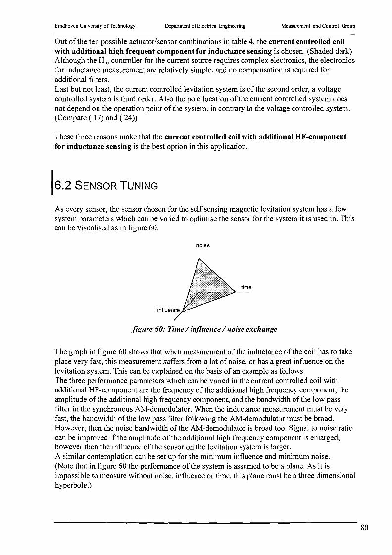
Eindhoven University of Technology Department of Electrical Engineering Measurement and Control Group
Out of the ten possible actuator/sensor combinations in table 4, the current controlled coilwith additional high frequent component for inductance sensing is chosen. (Shaded dark)Although the Hoo controller for the current source requires complex electronics, the electronicsfor inductance measurement are relatively simple, and no compensation is required foradditional filters.Last but not least, the current controlled levitation system is of the second order, a voltagecontrolled system is third order. Also the pole location of the current controlled system doesnot depend on the operation point of the system, in contrary to the voltage controlled system.(Compare ( 17) and ( 24))
These three reasons make that the current controlled coil with additional HF-componentfor inductance sensing is the best option in this application.
16.2 SENSOR TUNING
As every sensor, the sensor chosen for the self sensing magnetic levitation system has a fewsystem parameters which can be varied to optimise the sensor for the system it is used in. Thiscan be visualised as in figure 60.
noise
figure 60: Time / influence / noise exchange
The graph in figure 60 shows that when measurement of the inductance of the coil has to takeplace very fast, this measurement suffers from a lot of noise, or has a great influence on thelevitation system. This can be explained on the basis of an example as follows:The three performance parameters which can be varied in the current controlled coil withadditional HF-component are the frequency of the additional high frequency component, theamplitude of the additional high frequency component, and the bandwidth of the low passfilter in the synchronous AM-demodulator. When the inductance measurement must be veryfast, the bandwidth of the low pass filter following the AM-demodulator must be broad.However, then the noise bandwidth of the AM-demodulator is broad too. Signal to noise ratiocan be improved if the amplitude of the additional high frequency component is enlarged,however then the influence of the sensor on the levitation system is larger.A similar contemplation can be set up for the minimum influence and minimum noise.(Note that in figure 60 the performance of the system is assumed to be a plane. As it isimpossible to measure without noise, influence or time, this plane must be a three dimensionalhyperbole.)
80

Eindhoven University of Technology Department of Electrical Engineering Measurement and Control Group
In the levitation system under study, the bandwidth of the mechanical system is assumed to be100 Hz. This means that the low pass filter in the AM-demodulator must have a bandwidth ofat least 100 Hz.Further more the Nyquist criterion requires that the sample frequency is at least two times thehighest frequency to be measured. So this criterion demands that the frequency of theadditional high frequency is at least 200 Hz. However, because the band pass input filters ofthe AM-demodulator cannot be infinitely steep, the frequency of the additional componentmust even be as much as 1 kHz, to avoid noise caused by the actuating current.Finally, the amplitude of the additional high frequency component must be chosen. When theactuating current is zero, still a DC-voltage must be supplied to the coil to be able to sourcethe inductance sensing signal. The DC-current by this DC-voltage must be compensated forby the current through the opposite coil, and thus must be a small as possible. On the otherhand, when the inductance sensing signal is very small, the signal to noise ratio of theinductance sensor is very low.
Regarding the restrictions as stated above the three system parameters for the inductancesensor are chose as follows:
fHF
Blow passjilter AM-demodulator
Vinductance measurement, DC
Vinductance measurement, AC
iinductance measurement, DC
iinductance measurement, AC
= 1 kHz= 100 Hz= 1.5 V= 1.5 V=285 mA= 2.38 rnA
( 102)
81

Eindhoven University of Technology Department of Electrical Engineering Measurement and Control Group
7. CONTROLLER DESIGN
In the previous chapter the current controlled coil with additional HF-component was chosenas the actuator/sensor combination for the self sensing magnetic levitation system. This givesthe system as depicted in figure 61.
~ ~ L inductance induction ->H -
/ c measurement,
position
current source
i/
..L. 0- ~}- po,,;O"
+position,/ /
+'r-:' controller .......
HF-source
figure 61: Block scheme ofmagnetic levitation system
In chapter 4, section 4.1.4, the transfer function and phase shift form input voltage to outputcurrent of the current and voltage sensing Hoo controller is plotted. As already indicated, thebandwidth of the Hoo controller is much more than the bandwidth of the mechanical system.Abo the phase shift for low frequenc ies is very small. This means that the current source has aunity gain transfer function (in the concerned frequency band) and introduces no delay timeinto the levitation system.Further more, as the additional high frequency component in the current through the coil tomeasure its inductance is at least two time higher than the highest frequency in the mechanicalsystem (that means is at least 200Hz), the output signal of the inductance sensor does notsuffer from aliasing. Because operation of the sensor is continuous, the sensor does notintroduce a time delay into the system.So, the actuator as well as the sensor are designed such that they do not have any influence onthe transfer function of the magnetic levitation system, as derived in chapter 3.
When the model parameters, given in chapter 2, are substituted into the linearised transferfunction given in chapter 3 by ( 17) a controller for this linearised process can be designedusing several design tools, e.g. Matlab. The model parameters are summarised in ( 103)
x(s) !2ABge- BXo 1H(s) =- =- r-=i(s) ~ m (s + ~gB )(s - ~ gB)
82
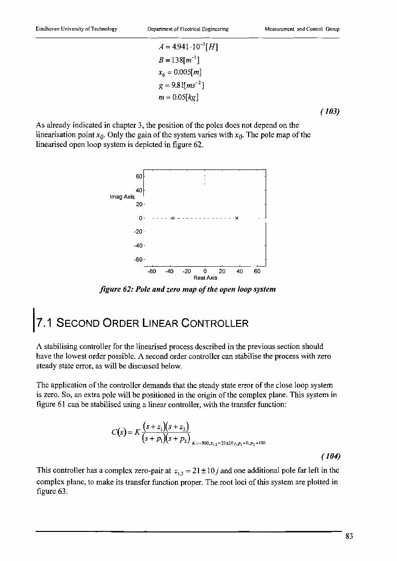
Eindhoven University of Technology Department of Electrical Engineering
A =4.941·1O-3 [H]
B =138[m-1]
Xo = O.005[m]
g = 9.81[ms- 2]
m =O.05[kg]
Measurement and Control Group
( 103)
As already indicated in chapter 3, the position of the poles does not depend on thelinearisation point Xo. Only the gain of the system varies with Xo. The pole map of thelinearised open loop system is depicted in figure 62.
60
40ImagAxis
20
Io - - - - - -x- - - - - - - -i - - - - - - -* - - - - I
-20
-40
-60
-60 -40 -20 0 20 40 60Real Axis
figure 62: Pole and zero map ofthe open loop system
jJ.1 SECOND ORDER LINEAR CONTROLLER
A stabilising controller for the linearised process described in the previous section shouldhave the lowest order possible. A second order controller can stabilise the process with zerosteady state error, as will be discussed below.
The application of the controller demands that the steady state error of the close loop systemis zero. So, an extra pole will be positioned in the origin of the complex plane. This system infigure 61 can be stabilised using a linear controller, with the transfer function:
( 104)
This controller has a complex zero-pair at Zl 2 = 21 ±10 j and one additional pole far left in the
complex plane, to make its transfer function proper. The root loci of this system are plotted infigure 63.
83

Eindhoven University ofTechnoJogy Department of Electrical Engineering Measurement and Control Group
, ,
Of--+---*
-20
-40
20
60Imag Axis
40
-60
-60 -40 -20 0 20 40 60Real Axis
figure 63: Rootlod ofcontrolled system, K- 900, ZI,2=-2lrlOj
When the zeros ofthe controller are located more to the right, the inner pole-pair would beless damped, so the zeros must be located as far to the left as possible. However, when the twozeros are located more to the left than that they are in figure 63, the outer pole-pair would goto the zeros in stead of the inner, and the latter pair would be much less damped. So theposition of the zeros in figure 63 is the optimum.The gain K of the controller is chosen at Kopt such that a line through the two poles with apositive imaginary part leads through the origin. (See dashed line in figure 63.) In that casethe system is damped optimal: When the gain K set lower than Kopt' the inner pole-pair wouldbe less damped than in the case K is equal to Kopt' and when the gain is set higher than Kopt'
the outer pole-pair would be less damped.Remarkable is that the gain of the controller is negative. This is because the process has also anegative gain. Physical interpretation of this phenomenon is that (when in equilibrium) thecurrent through the coil iL increases, the distance between the ball and the coil x decreases.
Note that it is possible that the gain K is such high that the actuator is not able to supply thedemanded current at aU times, or that the magnetic material of the coil saturates. This will beexamined in detail in section 7.5.
17.2 THIRD ORDER LINEAR CONTROLLER
Simulations (see section 7.5) show that the second order controller designed in the previoussection is not able to stabilise the non linear process. Therefore a third order controller whicheffects much more damping is designed in this section. Simulations show that this controllercan stabilise the non linear process. Formula ( 105) shows the transfer function of a third ordercontroller which can be used in the control scheme in figure 61.
( 105)
84

Eindhoven University of Technology Department of Electrical Engineering Measurement and Control Group
This controller has one zero at s=-40 to cancel one open loop system pole, two zeros at s=-60and two additional poles far left in the complex plane, so that its transfer function is proper.The root loci of this system are plotted in figure 64.
50o
200.------r----,---...,.,.-----.----,.---,
150
100ImagAxis
50
o
-50
-100
-150
-200 '-----_~__~_...J......o.__--'-__'-----'
-200 -150 -100 -50Real Axis
figure 64: Root loci ofcontrolled system, K- 2775, zl=40,Z2=Z3=60
A comparison between figure 63 and figure 64 shows that the poles of the closed loop systemare located more to the left in the complex plane. This implies that the system is moredamped.Disadvantage of a third order controller in comparison with the second order controller is thatthe former has an extra differentiator, and thus suffers more from noise.As with the previous controller, the position of the zeros and the gain of the controller areoptimised using a iterative process.
Note that again, saturation of the current source and the magnetic material of the coil core isexamined in section 7.5.
17.3 THIRD ORDER NON LINEAR CONTROLLER
In the previous two sections the root loci were plotted for the controlled linearised system inthe nominal operation point Xo (=0.005[m]) However, when the system is not in the nominaloperation point, but in x=x* the root loci of the controlled linearised system differ, as can beseen in figure 65.
85

Eindhoven University of Technology Department of Electrical Engineering Measurement and Control Group
50o
200 .---~--,....--..,.--,-----,-------,,.------,
150
100ImagAxis
50
o
-50
-100
-150
-200 '--_----'-__~_...l..._L___'___ ____'_
-200 -150 -100 -50Real Axis
figure 65: Root loci o/the controlled linearised system, around the nominal operation point
In figure 65 for x*=0.002 (point 1), x*=0.004 (point 2), x*=0.006 (point 3), x*=0.008 (point4) and x*=O. 010 (point 5) the root loci and the position of the poles are calculated, using thelinear third order controller of the previous section. One can see that the trajectory on whichthe poles are located does not depend on the operation point x *, but that the gain oftheprocess (and thus the optimal gain Kopt ofthe controller) changes significantly. It is thereforesensible to design a controller which takes the operation point into account.
Formula ( 17) shows that the transfer function(*) of the process can be described by:
1H(s, x) = A(x) ( )( )'s+ p s- p
( 106)
where:
( 107)
It is then easy to correct for the dependence of the gain on x by taking:
( 108)
and:
K(x)· A(x) =Gopt
( 109)
The relative difference in the gain of the linearised process in the operating x and the nominaloperating point Xo is:
86

Eindhoven University of Technology Department of Electrical Engineering Measurement and Control Group
J-B(x-xo)
=e 2
( 110)
This difference in the gain of the process must be compensated in the non linear gain of thecontroller. This gives the transfer function(*) of the non linear controller by:
C(s,x) = e~B(X-Xo) . [Ko
/ (s + 40)(s + 60)\s + 60)] = e~B(X-Xo) .[_ 2775 (s +40)(s + 60)\s + 60)]11 s(s + 140) s(s +140)
(111)
According to ( 14) a DC-current must be added to the output of the controller to set theprocess in the equilibrium point the controller is designed for. So, the current through the coilto levitate the ball is given by:
. 1211ig.I L =~~ + Icon/roller
( 112)
The technique described in this section, can also be applied to other linear controllers (Such asHoo-controllers, see next section.) to adapt them to the non linear process. This technique isalso known as exact linearisation. [16]In figure 66 the procedure of exact linearisation is plotted.
Non Linear Controller Non Linear ProcessEquilibrium
+ Linear Non Linear Current
IF-Non LineaRef ... Controller "1 Gain ~'"
i~
Gain 8 rt..inear Process '"',1'- '1+,
1/A(x) A(x),
Dfl'I
figure 66: Exact linearisation
(*) Formally this is not a transfer function. A transfer function does only depend on thefrequency (jOJ =s) and not the operation point x. Transfer functions must be linear.Nevertheless, in this report a transfer function multiplied with a non linear function whichonly depends on x is also called a transfer function.
87

Eindhoven University of Technology Department of Electrical Engineering
17.4 HCO -CONTROLLER
Measurement and Control Group
As with the current source (see section 4.1) an Hoo-controller can be designed for the processto find an optimal balance between noise reduction, overshoot, step response, actuatorsaturation etc. A non linear Hoo-controller will be designed in this section using the exactlinearisation scheme as described in the previous section. Therefore, a linear Hoo controllerwill be designed first and after that, this controller will be adapted to the non linear process.
In figure 67 the augmented plant is plotted for the system linearised in the operating point xo.( 103) The generalised plant is depicted in figure 68.
w
u.----t+----*9-~
figure 67: Augmentedplant
z
controller
figure 68: Generalised plantfor MHC-Toolbox
In figure 67 the plant is the coil, controlled by the voltage controlled current source, as insection 4.1, and the ball. The input of the plant is the input voltage of the VCCS, the twooutputs are the position of the ball, and the voltage over the coil. As already indicated insection 7, the voltage controlled current source and the inductance sensor have no influenceon the transfer function of the magnetic levitation system as derived in chapter 3. (In theconcerned frequency band.) This leads to the transfer functions of the plant P as in ( 113)
88

Eindhoven University ofTechnology Department of Electrical Engineering Measurement and Control Group
The plant has three exogenous inputs. The first is sensor noise, with its shaping filter VI I. Theposition sensor with its additional electronics is assumed to have a signal to noise ratio of atleast 60dB. This leads to VJJ=-60 dB=O.OOlThe second exogenous input of the plant is system noise, with its shaping filter V22. Systemnoise is added mainly for modelling coil saturation but also for modelling the signal to noiseratio of the electronics in the controller, and the influence of the high frequency inductancesensing signal. When the currents through the coil are not too large, the influence of saturationeffects is relatively small. V22 is chosen as: V22=-60 dB=O.OOlThe last exogenous input of the plant is the reference signal for the position, with its shapingfilter V33. The reference signal is assumed to consist of low frequencies only.
Finally it is assumed that: '1'lwII12,lIw2112,lIw3112 < 1
The plant has three exogenous outputs. First of all the current through the coil, with itsshaping filter WI I. This exogenous input is to model saturation effects of the magneticmaterial of the coil core. WI I is chosen at 0.33.Note that weighting filter WI I as state above does not guarantee that the input signal of thecurrent source is small enough to avoid saturation of the current source. It only gives an roughestimation of the output signals of the current source for designing the HC() controller for thelevitation system.The second exogenous output of the plant is the output voltage of the current source with itsshaping filter W22, to model saturation ofthe output voltage of the voltage controlled currentsource. The maximum output voltage of the current source is bounded by its supplied voltage,which is assumed to be 30V. This leads to W22=0.0333Note that, again, W22 gives no guarantee that the desired output voltage of the current sourcenever exceeds 30VThe last exogenous input of the plant is the tracking error of the ball, with its shaping filterW33. The tracking error must be small for low frequencies can be large for high frequencies.
Finally it is assumed that: !iZII12,llz2112,!lz3112 < 1
The transfer functions of the plant are: (Remark that the position of the ball is expressed inmillimetres rather than in metres)
1000~ I = _ 0.1 092s2 + 147.8048
P. _ 691s+2198012 - s + 6280
( 113)
The transfer functions of the weighting filters are: (Remark that the position of the ball isexpressed in millimetres rather than in metres.)
89

Eindhoven University of Technology Department of Electrical Engineering Measurement and Control Group
~I
~2
V;\ =0.001
V;2 =0.001
10.62.83
V;3 = 3(s+ 62.8)
1
31
30
30.6.284• (s + 6.28)2
W;3 = 2(s + 0.628)2(S + 62.8)
( 114)
As formula ( 113) shows, the plant is linearised in the operating point xo.The transfer functions ofthe plant and the weighting filters are plotted in figure 69.
P12
. 1111]
I1I111
'i I111
'III
: II,
111111
I I111I
1111I1
, 111\:
I I 1'1111
, 111I
'II
I1111
-1111111
I I ,III'
I 1 I i III:
" I111
I I lilli'
I I I II
I T II Ii'
I i 1111:1
I I" III:,
I 1111l
I I '_' I_"~ _
11111I 11
I II I1I11
I Iii 1111'
I 11I1II11
I 1111II1
I 1111I1I
I 111I111
I 11111I1
I Ilillll
11I1111
I 111\111
1I11I11
I I 111111' I I 111I111
'111111 I I 1I111I1
-1- 1-11'1111 -1-lllllljT-
I :11111 I I Illilll
I I I ililil I 11111111
I I 111I111
I I 111~11~_I_!-IJI11!..!._
I I 11111I1 I I 111I1I1 I 11111\1
I 1111I1I1 I 1'111111 I I! 11111
111:11 I 111111,
1II'IIil I I II I I i III
- 1- I-n ITIII - r r II ITI IT - ! T Ii fllT~
I I; 111111 I I I I1I1I1 11111,11
1IIIil I 1111111
102
Frequency radV33
I1IIII1 I I I IIIII1 I \ I' 1IIIi I IIIII!I
I1IIII1 I I1IIII11 I 1'1"'11
111111111111111111111"'/'111111- ,- rlilTl1i - r ril 111fT ~ TTl nl~ - T - fiT!
I I II1I11 I I IIII111 I I : I!I:I I' IIII
I I I I I I I I I I I I I I I I I I I I ~ II ~ I I;: I I I I I
I i I I I I I I I I I I I I I I I i I I I I I ' I ~ , I I I I I I I-1-'-I-illlll-III!llliT-TTI-'II I ;11111
I I 1111111 I I 11II1I1 I : I III: 11I1
111 111 I I I1II11 I I,ll" '11111
I 111111 I I I I1I111 I 1111I1I1 ,1111
11111111-111-111111 111I11I ' '11111
111111 11I1111 1111111 I I II!I
11I1111 I I 11'1111 I 1111111' I 11I1111
_1 __ IJIIII~ _ ~ ~I_"JI~ _ ~ ~ 1_llJl.iJ _ i ilill
1111111 I I I I! III I I II11111 I Ii 11I1
I 1111111 I I' .il!11 I 11111111 I Ii 1I111
i lilli' 1111111 I I I111111 I i'lllll
40
o
30
-50
-100
dB
dB50
illl
11,11:
111111'
1111"
IIII1
I1II1
I IIIII
illl 20, II L
, IIIII1
IIII11
1010' 10°
" ! I II
I I II ;111
;! IIIII
I1II111
IIIIII1
j IIIII1
! I1II1
II,n'n-"-Trifli
, I1I1I
I1II1I11
11 1 1111
IIII1II1
I I11I1111
, Illill
1 '1 1"
I I IIIIII1
I Ii 1.1111
IIIII1"II,
I 1111':1
101
102
103
Frequency 'adV11,V22
11111I1 1,1; 11111 1
, , 11',illl 1IIIili
I illill I: I!:'I
I 1111'11
I Illill'
I 1',11111,
11,1111 I I I
-1-'-li:'I!1 - r'11'llil
- :_ I_'..!.! .!...'II__ 1_ ,_ I ~ --'Ii lilill
I 1111'11
I I III'
; lilli'
I: 1I111 1IIIili
: i 11]11 1111I11
II jllil 11111'.
11'1111 I I 1111'1
11-1111 I 111111
I ~'_I:~I!..!. _.!... J. 1_liJ~1
I 1,1','11 ........ I 1I111
I I 1'11111 ......,,' i "I!I
11 1 '11111 "1 1 111 1
III: . :~'III
I! 111:1 I I I I i I II
I I'1' I 1111111
-1-- i-I"Tlnl- - I rlll"TllT
I I 1111'1 I I 1111II1
I I I II1111 I I 11111I1
I I 111111: I I 1I11111
I 11111'11 I I 1111111
I 1111111: I I 111'111
',lil'l , III
- :-' n In - T I II il n'111111 I 11111'1
1,11111 11111'1
I1III1 111111
060 f-..,....,...,.,.,.:,.,;:.,.::,..:_,..,..,...,..,.,..,.,,...... ,_,..,,.,.,1.,."_.,......,...,'.,.'..,:,..:''''I:I I I lilli' I III
I 111I111 I I 11 1111 I I II
111111 I I I: 1I111 I I 11'11
_1_ I_I..!.I.!.-II~ _ 1_ ~ I~ i III __ .!.- ~I UI.!J _ ~..!. I
I 111'111 I I,'
I I11I111 111111:
I I 1111111 11I1111
I I 111I1I1 Ilillll
-50
odB
-60.5
dB
-59.5
-61 '-:-.L-l...J....U.Ll!.L-----'-L.L'-Ll.l.l.l...:-L...L.L.Llll.ll...-...L.J....Ll.llill -150 '-:-.L-l...J....U.illL---l-U...LLl.LlL-L..lJ..LllL"---..L....l....Ll.WlJ
10° 10' 102
103
10' 10° 10' 102 103
10'Frequency rad Frequency fad
90

Eindhoven University of Technology Department of Electrical Engineering Measurement and Control Group
W22
102
Frequency rad
I I I 111I11 I I I II1111 I I II I 1111 I I I 1I111
I , 111I11 I I I II111I I I II11111 I I I 11111
I I 111I11 I I I tllill I I I111111 I I I 11111-
I- I~!IITII"I - I I (I ITT - T T I:TIITI- -; iT 1I111
I I I 111111 I I I 11111 I I 1111111 I I I 1IIIt
I I I 111111 I I1111 I I i I11111 I I I 1II11
I I I 111111 I I 11111 I I , 111111 I , Ilill- - - - - - - - - - - - - - -
I I I, I 111 I I 111I1 I I I 111II1 I I I 111I1, I111I1 I I 11111 I I I 1I1I11 I I I 11I1I
I I I I1I111 I I 1II11 I I I 1II1I1 I I 11111- - - - - -11111
- - - - - -I I
-I I I 1I11I1 I I I I I I 1II111 I 1I1II
I I I 1I11I1 I I I 1II11 I I I I tlill I I 11III
I I I 1I11I1 I I I 1III1 I I I 111[11 I I I 1111I
- I_,- I JILII.!... - L ~ I_ UI.!J - .!... .1 LI 1 11.11 - J J.1 IJ III
I I I 1,11111 I I I Ilitll I I I 111111 I I I 111I1
I I I 111'11 I I I 1III11 I I I 111111 I I I 1111I
I I I II1111 I I I 111I11 I I I 11111I I I I 11I11
-30
-29
-30.5
-29.5
-28.5
dB
W33
I I IIII1I1
I II 11111 I I I I I I II
III1I11 I IIIII11-----------I I III1I11 I IIIII11
I I IIIII11 I IIIIII1
I I II1I111 I I III1I1
_ J... J. Li .!...II ..U _ ...!. ...! 1 I...!. I II
I I I1I1I11 IIII!II
I I I 1111111
I 111II111 I I111II1
W11
102
Frequency rad
I I I IIIIII I I III1II1
I I Illilll I I III11I
I I I' I I I I
I I I I I 1'1
I I IIIIII1 I I IIIIII1
I I IIIIII1 I II11III1
_1_ U....!llilL _ 1_ LU UllJI I I IIIII1 IIIIII1
IIIII!I I I 1111111
'111111 I1III11
-10
I I I IIIIII I IIIIII I I IIIII11 I IIIIII1
I ! I III1II I IIIII1 I ',111111 I IIIIII1
I I I11I1I1 I I I I1IIII I IIIII11 I IIIIII1
-I~I-IIITIIT - r ,n(IIIT - T IlnlTI -"T'" TIIII
I I I I I I I I I I I I I I I I I I I I I I : I : ~ I I I I I I I I I
I I' ,11111 I I I I1III1 I I 1IIIIil I 1.111111
I I" II III f i I I I IIII I I I I i IIII I I I I, II II-9.5 F--"--t'-:....,-o.-,--,...-"'-'---~- ....-"'-,.....,--ii'-...::-'---~- -i"-;-f-:'-'-;;""'::'-":;-"'::-""-'i'+'--'""I
-10.5
-8.5 '-"""TT!"rrrr--,----r-rrnrrr--r-T"TT1"TT1'r---r...-r.,..,-rrn
dB
-9
dB
o
-50
1111II1 111111
111I111 II1111
1I1II11 II1111
11111I1 I 1111111
I I I11I1111 I 11II11I
__ 1_111.!...11!.... _ L L L 1 U Ull.! _ 1 J 11.1..11 1
I: 111I11 I I I 1111111 I I: III
I I I111111 I I 1I111 1I1111 11111
1111111 I I 111I1 II 1111 I1111
111I111 I 1I111 11I1 I1I11
, 1,,1'11 1I1I1 I 111I111I I I III
I 1111111 I I I 11111 I IIIIIII! 11111
-1-r-ITlrllr-rrllliIIT-rTrlnITl-T ITI
1 ',11111 I 11111111 I I II ilill I I I I
I It I ',II I I I I I II II II 1111I I I I I
I I I I I I III I I I I I II II I II 11111 I I I I I
I Ii 11I111 : 1111I1 I 1111111' I 11I11
I111111 '11'111 I 1IIIIIIi I I111111
-1 00 I...-J......l...J...J...L.l..W._'---'-.J....U..ll.ll.----'--'-l....W..WJ......J...J.......l...J...llJ..UJ
10° 10' 102
103
10·Frequency rad
figure 69: Weightingfiltersfor MHC-Toolhox
When a controller is designed using the weighting filters as in ( 114) MHC gives the results asin figure 70. The solid line is the transfer function from a certain input of the augmented plantto a certain out. The dashed line is the boundary of stability. The optimum for ywas found tobe 1.138, which is close to 1, as it should be.
100Closed Loop output voltage by sensor noise (1->2)
dB50
30
lilli' I I 111 ' 111 ',111111 I 111I1I1
I I 1111111 I I 11111 1IIIili
I I 1111111 I I I1111 I1I111I 1111111
I I 1111I11 I I ; 111I I I I! I111I I 11I11I1. -1-1-1111111 - 1"1 Illii - T 11111111- ,-\ I1I111
I I 1111111 I I .1111 1111111 I 1111111
I I 1111111 I I ;111: I 1111111
[ 111111 I I ilill I 1111111
I I lilli' I I I 1111111
11-1111111-11 I 111111
"1111 I I 1I1111 I 1111
I111I11 I I 1'1111 I II, II
11 1111 I I 111111 1111'11
'IIJ..IIJ... _!.... !... I_I I---.!IU _.!..! _1J..1Ill_ J J .!IJIII
I 1111II1
111II1
111;11
I 1111111
dB
50
o
I-----.!-!--U-l-III---- l..---l.-1-l-l-l1W-- L....l-- ~14- w.J..11
I 11I1I1I1 I I 1111111 I 11 I 1111 I 1111111
I I111I111 I I I111111 I I III !I 111111
I I I II11I1 I I I 111111 I II 1111 I 1111[11
I II1111 I I 111I1I1 I I11111 111I11
___ I.!I.!...II.I- _1_ !""IJ.IJ..II.!. _.I- I_I iJI!.!. _.!..l U.!...!III I I I III I I I I I 1111 I II I1111 I I I I I II
I 1111111 I I I III111 Ii 1111I1 I11111
1111111 11111111 I 1IIIIIil 111111
1111111 I II1I II ilill Ii 111I
I 1111111 I I I III I 11111[11 1I1111
1 1111II1 I I11111 I 11111111 I 1II1111
- 1- !-I Tin II - r IIITI rr - r r II n lIT - T T rI n I
I I [Itlill I 1111111 I 111II111 I I111I11
I I 11111',1 I 1111111 I Illillll I 1IIItii
111I111 I I11I111 11I1I1I I I I: 1111
I 1111111 11I11111 I 11111"' I 1I1I1I1
I1111111 I 1',111111 I 11111111 I IIIIII[
20 '-:-.....................-'..UJ..-:-'--'-w..u~---'-...l....l..u..w.J.L.-...l.-LLl..LLl.lJ -50 L-.L...L.LllillL---L--'-'-'-J..J.llL--L.-.L..LJ-illiL.-.l-L...J..J...I.wJJ
10° 10' 102 103 10· 10° 10' 102 103
10·Frequency rad Frequency rad
91

Eindhoven University of Technology Department of Electrical Engineering Measurement and Control Group
Closed-loop position noise by sensor noise (1->3)
I I 1II1I11 1 11I1I111 I 11111111 I1 1 1111
I I I \llill I 11I11I11 I 1IIIilii I 11)./'111
Illllllil 1IIIIilii 111111111 1/11',111
-1-rll"lnli -, iillllrT - T T ilnln71 l" IiTI
I 11I11111 I 1 11I1111 I 1111-1"i"I1 I I 1111,1
111111111 i 11111!11 I nillill 11111,11
1IIIilili 1111117 .---(11111111 I 111'11
- i- 1-1111111 - ....c.....i-Hiil;l - 'I T II lilT! - T I" Ii I11I
1/ n"I~ I~ I I I I 'I I I I I " I I I I II I I I , , I II
I i I lilli' \ I I11111 I 11111111 1111II1
I I I I I I I 11I11111 111I111
- II1I - 1IIIIIilj -I II1I111
~i!---'--l...u""""""-.l"";1 II I III I I I I 1 I I I t
I I I II1111 I I
__ 1_lll.!...ll.!.... _1_ l-1-.!iJ.I!.i. _ ~ l U!....II~_
I I I I11111 I I I illill I I11I111
"lllill I I 1111111 I I1I1I11
I I 1111',1; I I: II-III ,1111
o
50
-50
Closed Loop position noise by system noise (2->3)150 ,-----~..,.....,.,..".,...~....,....,.~...,.-....,....,.T""T"'"""'"""',..._~...,...,..,.,..,."
-1 00 L-.L.....L.Llll.l.U-----l.--l....L...Llllll---'--.L.W..llllL-----l...u..J.llJJ
10° 101 102 103 10·Frequency rad
Closed Loop tracking error (3->3)
dB100
III,'
'II
111\11
I "
I I 11111,1
1\11111
')/ "/ IIIII111
I I II I
, "
I I IIII1
',111111
I :11 II- -: I
IIIIII1
'1 'II
I I 11;1111
I I I IIII 11,1,;
jllill I I: 11111,
) I ililll I I 111',11'
. - - l~il','111 -'I T I-I
I I 11111t) I I 11:lOi,
I I I I I1II I I III I
I 11,1:,1 : 11'11'
I I III I
I:]' ~
I~I ;11,,1
v-I I I II !II I I I
I !IIIII 1'11111
101
102 103 10·Frequency rad
Closed l.oop output voltage by reference (3->2)
I illli
I III~
11../'11 11 1
£_1 ~ I~ I~II \ III111
I I 111011
IIIII1
II jill
I IIIII1------I '111111
I 1111'11
I III1II1
I I: I illl
of---,---,---,-'!,;I'.!o'.!o'_.!-.w"':":'=_-'--.J....u.,;=-.".--, _I J IJ IIII I I IIIII1 I I I' I I 1'111,1 I I: I11I
I 1'1"11 : I 1"1 I1III11
IIIII!
IIII I
150
50
100
150
dB
of---'-_'_-_'-_.,.,..--
I I Illilll I I I !lllli I 111111',1 11 1 I1
I I1I11I1 11111111 1IIIIIIIj Ilyll
: :: II ~~,: : : : :::: II::: ::::: : ':~:::::1IIIIIIil 1111111I1 I11111111 VI 111111
_11- --:~:~::~ - ~ ~IIJt:~:~ _l } ~:~:';~7f ~ ~:~:::11111111' 1I11I111 1111.01 IIIIIII!
:: ::::::11 I 1:111111 :: ~::::: :: :;:'1::
'11111 I 1111I11 1/' 11II11 1I1111
_:_II_:~:~I:~ _ ~ ~:~';~I,~ fi
~ ~~ II:~ I Ii 1111
I I 11I1111 I 1\1101
'I 11,1 ':1I 11III111 I III II
, I I i III" I I I ,II
o
100
dB
I 1111\1
~--'- _ J ---' J. 1'1'.1111
I I'll
III III
IIII!III I I III I
I : : : :::: :: ({:: :~,II I I 1:','11 1/1' I 11111
,,- TIIIIIIII-J:'! 111-1111
I I Ii lil]l I I
I "Iill
I lilli',
I 111111,
II I
I I I
I1111',1'
1111:1
I I 1IIIil- 1- 1-'- 11,1
"'I
'11111
I 1IIIi\:
I I II1I11
I 11111::-1- ,- 1111'1
I 11',1
I
50
dB
100
II I I Iii I ill : II!!II
-50 L-.L.......LU.J.ll.c--'-L~~L~--'-.w..;.;."---...L-'--LL~ -1 00 L-L...!...L.....=---'---l....L...l.ll"'---'--.L.W--'-'-"~-L.....--'.J.J..J
10° 10' 102 103 10· 10° 10' 102 103 10·Frequency rad Frequency rad
figure 70: Controller designed by MHC-Toolbox
The upper left plot in figure 70 shows the transfer function of the controller. The controller isof the tenth order.The upper right part of figure 70 shows the bottle neck of the system for high frequencies. Theplot of bottom left part shows the bottle neck for frequencies around 100Hz. Apparently, themaximum output voltage of the voltage controlled current source is for high frequencies thelimiting factor for the system. This can be understood by the fact that the output voltage is thethird(!) derivate ofthe position.The tracking error for low frequencies is -60dB (0.1 %)For all frequencies system-noise 1S damped very well.
In figure 71 the rootloci of the system controlled by the Hoo-controller are plotted. The plot onthe right is an enlargement of the shaded area in the left plot.
92

Eindhoven University of Technology Department of Electrical Engineering Measurement and Control Group
systempoles
50-200 -150 -100 -50 0Real Axis
o-1000 -500Real Axis
20001..----~---~---____",___,
1500
-200u---------'-----'--------'>.L-J-1500
figure 71: Rootloci ofthe Hwcontrolled system
Until now the designed Hoo-controller was a linear controller. However, like with the thirdorder linear controller designed in section 7.2, a non linear Hoo-controller can be designedusing exact linearisation. The same non linear functions as in section 7.3 can be used. Thisgives the following transfer function(*) for the non linear Hoo-controller:
c{ )- B(x-xol. H ( ),s,x -e Ji1lH -co1l/roller's. ~
( 115)
Again the process must be set in the equilibrium point the controller is designed for. Thereforea DC current must be added to the output of the controller. So, the current through the coil tolevitate the ball is given by:
. I 2mglL = ~ ABe-Bx + ico1llroller
( 116)
(*) Formally this is not a transfer function. A transfer function does only depend on thefrequency (jm =s) and not the operation point x. Transfer functions must be linear.Nevertheless, in this report a transfer function multiplied with a non linear function whichonly depends on x is also called a transfer function.
93

Eindhoven University of Technology
17.5 SIMULATIONS
Department of Electrical Engineering Measurement and Control Group
In this section the non linear process controlled by the various controllers designed in theprevious sections is simulated, using Matlab 4.2c.l with Simulink.
Although a certain DC-current iogiven by ( 14) necessary to keep the process in its operating
point, preliminary simulations show that, to stabilise the process, the control current T canexceed io in the negative direction. This means that in those situations in spite thegravitational force the controller wants to 'push' the ball away from the upper coil. However,because the electromagnet can only 'pull' at the ball, the control current must flow throughthe bottom coil, in stead of the upper coil. [11] This gives the control scheme as in figure 72.
in
Selector Amplifiers
figure 72: Two-coil-control
When simulating the two-coil-control scheme as in figure 72 one can use the followingoperation for the square in ( 7)
1 -B.x.2 (. )I' =- - AB· e . 1 • sgn 1
Jill 2 L L '
( 117)
where1m is the total magnetic reluctance force on the ball by the two coils and iL is thecurrent through (one of) the coils.
Using ( 117) gives the Simulink model as in figure 73, figure 74 and figure 75 for thecontrolled non linear system.
94
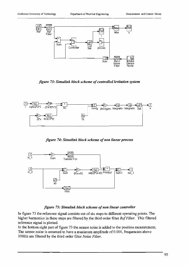
Eindhoven University of Technology Department of Electrical Engineering Measurement and Control Group
Controller proces
SensorNoise
figure 73: Simulink block scheme ofcontrolled levitation system
xSatfm+fg (fm+fg)lm
ffg
figure 74: Simulink block scheme ofnon linear process
11-----.......>/'\:::>----*'::"+11----------,In_1
B'(x-xO)
xOXO
L- ~ f U }-- ---J
iO(x)
figure 75: Simulink block scheme ofnon linear controller
In figure 73 the reference signal consists out of six steps to different operating points. Thehigher harmonics in these steps are filtered by the third order filter RefFilter. This filteredreference signal is plotted.In the bottom right part of figure 73 the sensor noise is added to the position measurement.The sensor noise is assumed to have a maximum amplitude of 0.001, frequencies above100Hz are filtered by the third order filter Noise Filter.
95

Eindhoven University of Technology Department of Electrical Engineering Measurement and Control Group
The measured position of the ball is subtracted from the reference signal, and then supplied tothe controller. The block scheme of the (non linear) controller is depicted in figure 75.The output signal of the controller is clipped at +4A (upper coil) or -4A (bottom coil) by thesaturation block, to simulate the saturation of the coil. (Magnetic hysterese is not modelled.)The output of the saturation block supplied as the input signal of the process. The blockscheme of the non linear process is depicted in figure 74.
In figure 75 an additional gain block is added in series with the linear transfer function of thecontroller. This is because the input signal of the Hoo controller designed in section 7.4 wasexpressed in millimetres rather than in meters. Also, as already indicated in chapter 2, the gainof the process is negative. Therefore this amplifier block must have a gain of -1000.
In figure 76 the simulation with the third order non linear is depicted. The plot on the left isthe position of the ball, the plot on the right is the current through the coil. Obviously thecontroller cannot stabilise the ball very well: High frequencies are poorly damped. (Thesecond order controller, and the linear third order controller are unable to stabilise the ball atall.) In the reference signal all frequencies above 15Hz are filtered by the reference filter.
32
5r-----.-:----r-:-~ I
o l _
_51------'----~--_....J
o
0.01 r------,-------.------.,
l008 ---- ----- ---: ------ ------;- --- ---~ ~-__ -~ I t rF
:::: :h:h~]: --:::1.~,::-r~J::::l002 ----- -~ ----l----j'-'- -- --;- ------- ----
:~ :o . ""_~_~__.__.l~_____'o 1 2 3
figure 76; Simulation o/the tMi'd order non linear controller
In figure 77 simulation of the non linear Hoo-controller is depicted. One can see that thetracking of the reference signal is very well. In the reference signal all frequencies above15Hz are filtered by the reference filter. The current through the coil never exceeds thesaturation value of approximately 4A.
96

Eindhoven University of Technology Department of Electrical Engineering Measurement and Control Group
0.01 5.------.....,...-------,r-------,
),008 ------- -- ---c - - -- - - - -- - --,- - --- --- - - --
32
,. ,, ,o ------------~------------~-----------
,,,,,,,,,,,,-5 L-__-----''----__-----'' --l
o32
),006 ,,..~ :
::::: ::::::~:r:::f:: :.:::::::::::0'-----'-----'---------'o
figure 77: Simulation ofthe H 00 non linear controller
In figure 78 the Hoo-controlled process is simulated, when a reference signal is applied abovethe design criteria of the Hoo-controller. (Note that for visibility the time axis is expanded afactor three.) Now in the reference signal all frequencies above 50Hz are filtered by thereference filter. This leads to more overshoot in position of the ball, and the current throughthe coil saturates.
0.01 ,---------,---------, 5,--------,-------,
),008
If
10.5
,o ------------------~ -----------------
,,,,,,,
-5 L- ----'-' ---'
oo-.--------.:-.----------'o 0.5
),006 1\ - -- -- - - - - - - - - - - -- ~- ----- -- - - - - - - ----I ,
J.OO4 ----- -- --- --- -----L::----- ---J.002 ----------. ---_. -- ~ -----------------,,,
figure 78: Simulation ofthe H oo non linear controller,frequencies above specs.
In figure 79 the Hoo-controlled process is simulated, when noise is added to the positionmeasurement signal. (Note that for visibility the time axis is expanded a factor three.) Asstated before, the maximum amplitude of the noise is O.OOIm, and it is low pass filtered by athird order filter at 100Hz. One can see that the coil does saturate. Sensor noise has a verylarge influence on the performance of the controller.
0.01 ,--------,---------,
(
....... p,t."',J/"\"""\J.004 ----- -- ---'" ---- -~ \( --- --- --- _. -- --
: y""'tP{y" ''iV 6:J' ¥
J.002 /-----------·-----i------------------,
0-· .:. ...J
o 0.5 1
5,--------,-------,
0.5
o
-5 L- ---'- ----'
o
,,,,------------------,------------------,
,,,------------------~------------------,
J.008
J.006
figure 79: Simulations ofthe Hoocontroller, noisy position measurement
97

Eindhoven University of Technology
17.6 CONCLUSIONS
Department of Electrical Engineering Measurement and Control Group
In this chapter a non linear Hoo controller is designed for controlling the magnetic levitationsystem. The controller was designed for the linearised system, and then adapted to the nonlinear system using a technique called exact linearisation. The performance of the designedcontroller has been examined by simulating its behaviour in the non linear process. Theperformance of the designed controller has been compared to linear and non linear PIDcontrollers.It appeared that the designed non linear Hoo controller was able to stabilise the position of theball very accurate. However, noise deteriorates the performance of the controller.
98
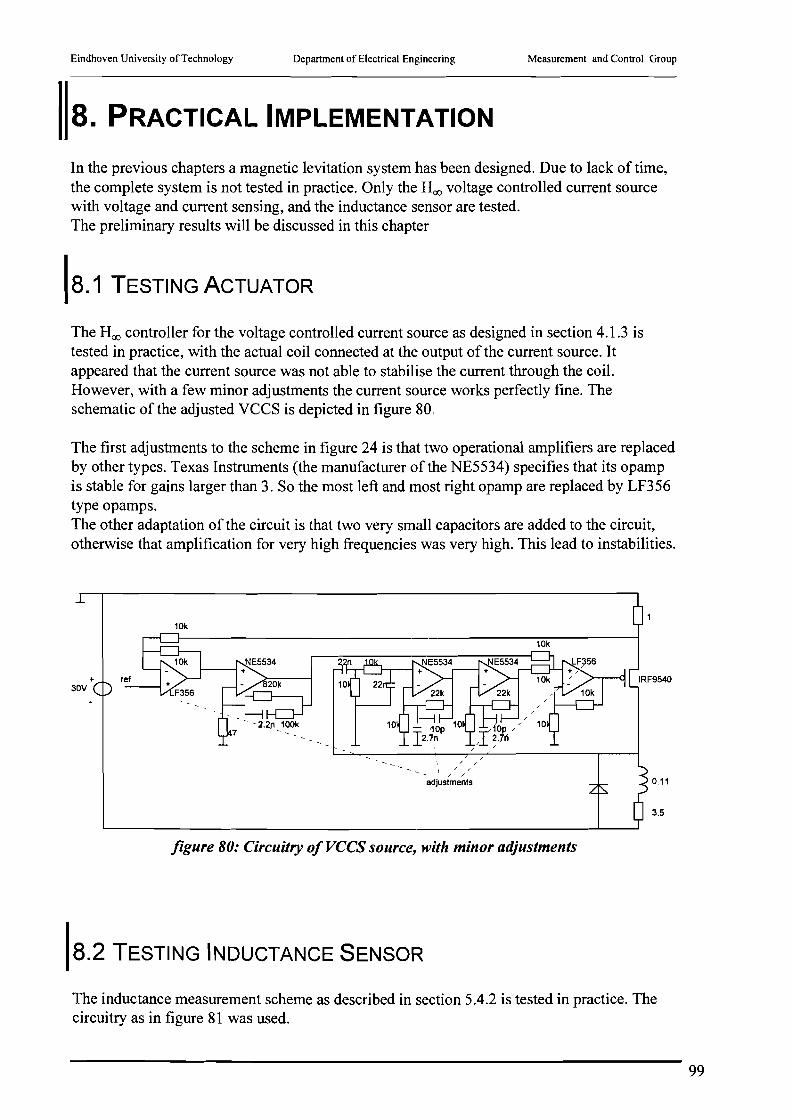
Eindhoven University of Technology Department of Electrical Engineering Measurement and Control Group
8. PRACTICAL IMPLEMENTATION
In the previous chapters a magnetic levitation system has been designed. Due to lack of time,the complete system is not tested in practice. Only the Hoo voltage controlled current sourcewith voltage and current sensing, and the inductance sensor are tested.The preliminary results will be discussed in this chapter
18.1 TESTING ACTUATOR
The Hoo controller for the voltage controlled current source as designed in section 4.1.3 istested in practice, with the actual coil connected at the output ofthe current source. Itappeared that the current source was not able to stabilise the current through the coil.However, with a few minor adjustments the current source works perfectly fine. Theschematic of the adjusted VCCS is depicted in figure 80.
The first adjustments to the scheme in figure 24 is that two operational amplifiers are replacedby other types. Texas Instruments (the manufacturer of the NE5534) specifies that its opampis stable for gains larger than 3. So the most left and most right opamp are replaced by LF356type opamps.The other adaptation of the circuit is that two very small capacitors are added to the circuit,otherwise that amplification for very high frequencies was very high. This lead to instabilities.
3.5
0.11
/ /
/ /- / /
adjustments
+30V
10k
figure 80: Circuitry of VCCS source, with minor adjustments
18.2 TESTING INDUCTANCE SENSOR
The inductance measurement scheme as described in section 5.4.2 is tested in practice. Thecircuitry as in figure 81 was used.
99
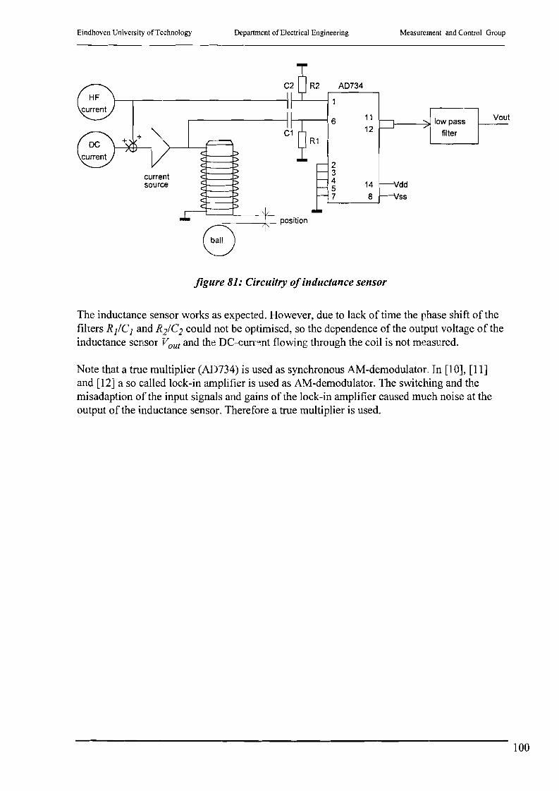
Eindhoven University ofTechnology Department of Electrical Engineering Measurement and Control Group
Vout
Vdd
Vss
I--_~ low pass
filter
11
12
14
8
2345
1 7
R2 AD734
R1
- -t position
8
,.-----------11--,-----1 6
currentsource
figure 81: Circuitry ofinductance sensor
The inductance sensor works as expected. However, due to lack of time the phase shift of thefilters RjlCJ and R2/C2 could not be optimised, so the dependence of the output voltage of theinductance sensor Vout and the DC-cun~ent flowing through the coil is not measured.
Note that a true multiplier (AD734) is used as synchronous AM-demodulator. In [10], [11]and [12] a so called lock-in amplifier is used as AM-demodulator. The switching and themisadaption of the input signals and gains of the lock-in amplifier caused much noise at theoutput of the inductance sensor. Therefore a true multiplier is used.
100

Eindhoven University of Technology Department of Electrical Engineering Measurement and Control Group
9. REFLECTING ACHIEVED GOALS TO MIRROR
DEFLECTION SYSTEM
As already indicated in chapter 1, the levitated ball as described in this report, is a pilot projectfor a magnetic levitated mirror. In this chapter the achieved goals for the ball will be reflectedon to the magnetic levitated mirror.
The magnetic levitated mirror for the laser deflection system has five degrees of freedom(DOF): three degrees for the position ofthe centre point of the mirror (x, y, z); and two for the
angle of the mirror (e, rp). See figure 82.
figure 82: Degrees ojJreedom ojmagnetic levitated mirror
In the application the mirror is used for (a laser interferometer), both the position and theorientation ofthe mirror must be known very accurately: the accuracy of position of themirror determines the accuracy of the laser interferometer (distance), and the accuracy of theorientation of the mirror determines the accuracy ofthe 3D-measurement of the position ofthe object.In contrary to the accuracy, the bandwidth and tracking ability specifications are very differentfor the position and the orientation ofthe mirror. First of all, the position of the mirror mustbe the same at all times. This leads to high noise reduction in a broad frequency bandwidth,but no tracking requirements of a reference signal. The bandwidth and tracking abilityrequirements of the orientation on the other hand are very stringent.This leads to the following observations or recommendations for the mirror levitation system:
1. In the current levitation system for the ball, I-shaped coils are used. In this case only afew flux lines lead through the ball, but most of them go around the ball. This leads tolarge Ls and small Lm, which means that the induction of the coil is very large, and thatthe induction is only slightly dependent of the position of the ball. Because of this themagnetic reluctance forcefm' is very small compared to the current through the coil iL>and the sensitivity of the coil as sensor is poor.It is much better to use U-shaped coils to levitated the ball (and the mirror). This willsolve the above problems.
2. To levitate the mirror, a large current is needed. This leads to saturation of the magneticmaterial and excessive heat production in the coil windings. The current necessary for
101

Eindhoven University ofTechnology Department of Electrical Engineering Measurement and Control Group
levitation can be (much!) smaller when the mirror is close to the levitation magnets.(~1 J.lm)For the orientation ofthe mirror a large air gap is inevitable. However because theinertia of the mirror is much smaller than the mass of the mirror ( 118), a smaller currentis needed for the same tracking error and bandwidth.
( 118)
where m is the mass of the mirror and r the radius of the half sphere mirror.
3. The mirror levitation system must be much smaller than the current ball levitationsystem. This will lead to scaling of the dimensions of the system in all three directions.The mass of the ball (mirror) will decrease with the third power of the scaling factor, thearea of the coils with the square of the scaling factor. This will lead to less saturation ofthe coils, and better heat radiation. Also, this will lead to a faster system.
4. In the current levitation system the material of the coil is ferrox cube. This materialsuffers form saturation at low flux densities (~O.lT) When weak iron (>99.98% Fe) orsilicon iron (SiFe) is used as the core material for the coil, the coil will suffer much lessfrom saturation (~1..2T) (See also section 2.1)Furthermore, in the current levitation system the ball to be levitated is a steel ball. Steel«99% Fe) has poor magnetic properties. It is better to use a weak: iron, silicon iron orferrox cube ball. In that case the magnetic reluctance force exerted on the ballfm at acertain current iL is much larger. Also the influence of the position of the ball x on theinductance of the coil L would be much higher.Note that to avoid Eddy current losses, the coils must be laminated or sintered whenusing weak iron or silicon iron. The ball nor the mirror must not be laminated becauseelse they would be anisotrope
5. More research is needed to examine the saturation characteristics of the magneticmaterial of the coil. It is unknown (at the section MBS ofthe TUE) whether saturation istemperature dependent, frequency dependent, time dependent, etc. When this is all notthe case saturation can easily be compensated for by using a look-up table.
6. Also hysterese of the magnetic material of the coil must be examined in detaiL Maybehysterese can be eliminated by adding a high frequency current to the actuator current.Note that this is already the case because of the inductance measurement.
7. Biggest problem of the magnetic levitated mirror for the laser interferometer is tomeasure the position (and orientation) ofthe mirror sufficiently accurate. Up till nowthis is done by measuring the inductance of the coil. (self sensing) Apart from saturationand hysterese, there is one other major problem: the inductance of the coil changes onlyvery slightly when the mirror (or ball) moves.Using the parameters of the current levitation system, the necessary accuracy of theinductance measurement is calculated as follows:
102

Eindhoven University of Technology Department of Electrical Engineering Measurement and Control Group
K
,ix = 10 .10-3m~ M = 4 ·1 0-3 H ~}
,ix =1·1O-6 m~ M =4.10-7 H accuracy.L =O.l000004H
L =100.10-3
"( 119)
Formula ( 119) shows that the inductance of the coil L must be measured with 7(1l!)significant digits. This must be considered as impossible, all the more because of theeffects of saturation and hysterese.
An other way to measure the position ofthe ball is to use a capasitive sensor as in figure83.
figure 83: Magnetic levitated ball with capasitive sensor
Because no additional wiring to or from the ball (or mirror) is desired, one cannotmeasure the distance between the ball and the coil by sensing the capacity of thecapacitor formed by one capasitive sensor as one plate and the ball as the other plate.Therefore two capasitive sensors are needed. The two capacitors are serie connectedthrough the (conducting!) ball. Those two capacitors cannot lie on opposite sides of theball (e.g. not sensor 1 and 3 or 2 and 4 in figure 83) because then the position of the ballhas no influence on the capacity of the serie connection of the two capacitors. (See (120), where K is a constant determined by the geometry of sensor and ball, x is thedistance between the first sensor and the ball and a-x is the distance between the secondsensor and the ball.)
K KKc- x a-x = _
- K K x+a-x - a-+--x a-x
( 120)
However, when the capacity of the four capacitors formed by the serie connection ofsensor 1 and 2, 2 and 3, 3 and 4, and 4 and 1 are measured, the position of the ball canbe calculated in 2D, using a formula which will not be derived here.
An other possibility to use capasitive position measurement (which can only be used forvery small gap widths is depicted in figure 84. The capacity between the bar "in themiddle ofthe sensor and its shield (shaded in grey) is influenced by the position of themirror. When designed correctly the inductance of the wires compensates the capacity
103

Eindhoven University of Technology Department of Electrical Engineering Measurement and Control Group
between shield and conductor in the wire (as with coaxial cables). So the capacity iszero when the mirror is very far away. (ideally)
sensor mirror
figure 84: Alternative capasitive sensorfor magnetic levitated mirror
Position measurement based on capasitive sensors can be much more accurate then theinductance measurement principle.
104

Eindhoven University of Technology
LITERATURE
Department of Electrical Engineering Measurement and Control Group
[1] Vischer, D. and H. Bleuler.A New approach to Sensorless and Voltage Controlled AMBs Based on NetworkTheory Concepts.Magnetic Bearing. Proc. 2nd
• Int. Symp. (1990), p. 301-306July 12-14, 1990, Tokyo, Japan.
[2] Mizuno, T. and H. Bleuler and C. Gabler and D. VischerTowards Practical Applications of Self-Sensing Magnetic Bearings.Magnetic Bearings. Proc 3rd
• Int. Symp. (1992), p. 169-175.Technomic Publishing Co., Inc., Lancaster.
[3] Vischer, D. and H. Bleu1er.Self-Sensing Active Magnetic Levitation.IEEE Transactions on Magnetics, Vol. 29 (1993), No.2, p. 1276-1281.
[4] Mizuno, T.Phase-Locked Loops for the Stabilization of Active Magnetic Suspensions.JSME International Journal, Series A, Vol. 37 (1994), No.3, p. 499-503.
[5] Bleuler, H. and D. Vischer and G. Schweitzer and A. Traxler and D. Zlatnik.New Concepts for Cost-effective Magnetic Bearing Control.Automatica, Vol. 30 (1994), No.5, p. 871-876.
[6] Kurita, Y.Displacement-Sensorless Control Using Electromagnets (Vibration Control by Currentand Magnetic Flux Feedback).JSME International Journal, Series C, Vol. 38 (1995), No.2, p. 233-239.
[7] Jayawant, B.V. and R.J. Whorlow and B.E. Dawson.New transducerless magnetic suspension system.lEE proc.- Sci. Meas. Technol., Vol. 142 (1995), No.3, p. 255-261.
[8] Mizuno, T. and H. BleulerSelf-Sensing Magnetic Bearing Control System Design Using the Geometric Approach.Control Eng. Practice, Vol. 3 (1995), No.7, p. 925-932.
[9] Sivadasan, K.K.Analysis of Self-Sensing Active Magnetic Bearings Working on InductanceMeasurement Principle.IEEE Transactions on Magnetics, Vol. 32 (1996), No.2, p. 329-334.
[10] J.H.H. Kop, A Magnetic levitation system, Master Science Thesis, EindhovenUniversity of Technology, Department of Electrical Engineering, Measurement andControl Group.
105

Eindhoven University of Technology Department of Electrical Engineering Measurement and Control Group
[11] MoL. Thijssen, A 2-dimensional magnetic levitation-system, Master Science Thesis,Eindhoven University of Technology, Department of Electrical Engineering,Measurement and Control Group.
[12] P.B. Houtkamp, Preparatory study ofa two axis mirror deflection system withmagnetic bearings, Master Science Thesis, Eindhoven University of Technology,Department of Electrical Engineering, Measurement and Control Group.
[13] A. Vandenput. Elektromechanica en vermogenselektronica, College diktaat,Eindhoven University of Technology, Department of Electrical Engineering, EMV.
[14] G.G. Persoon. Cursus Modeme Analoge Electronica. Phase-Locked Loops. Collegedictaat, Eindhoven University ofTechnology, Department of Electrical Engineering,SES.
[15] Heinz Falkuso Multivariable Hoo Control Design Toolbox User Manual, EindhovenUniversity of Technology, Department of Electrical Engineering, MBS.
[16] T. Sugie, K. Simizu, and 1. Imurao Hoo control with exact linearization and itsapplication to magnetic levitation systems. IFAC, Vol. 4, pages 363-366, 1993.
106

Eindhoven University of Technology Department of Electrical Engineering Measurement and Control Group
ApPENDIX A. MEASUREMENT OF SATURATION
OF MAGNETIC MATERIALS
ferrox-cube:
~ 0.0l1li
0.08 2.00.16 3.80.22 5.250.26 6.250.30 7.200.34 8.050.43 10.20.47 11.20.53 12.50.60 14.50.67 16.00.74 17.90.81 19.50.85 20.50.88 21.20.94 22.81.00 24.01.06 25.51.15 27.81.21 29.01.28 30.51.36 32.51.43 34.21.51 36.51.56 37.81.62 39.51.68 40.01.80 42.71.90 45.51.99 47.52.07 49.52.16 52.02.23 53.52.32 54.92.41 57.52.49 59.52.55 60.52.64 62.02.72 62.52.80 64.22.89 65.53.01 66.53.13 68.53.25 69.53.39 71.03.51 72.0
3.713.843.994.264.374.484.584.714.804.915.024.854.784.654.554.454.354.164.043.923.683.473.363.173.052.912.822.652.462.242.121.961.841.751.611.471.301.140.920.820.650.460.330.140.00
72.574.075.077.878.279.580.581.582.082.683.882.181.980.880.079.078.076.575.574.272.070.269.066.566.064.062.560.557.853.050.046.543.540.538.034.530.527.521.819.215.511.07.403.050.0
107

Eindhoven University of Technology
Steel-37:
Department of Electrical Engineering Measurement and Control Group
IU'I'PUU\ ,··.~Vl'fmm
0.00 1.00.02 1.50.04 1.80.06 2.20.08 2.60.11 3.20.13 3.60.14 3.90.16 4.20.18 4.60.20 5.00.22 5.50.25 6. I0.27 6.60.29 7.00.32 7.60.35 8.10.38 8.80.40 9.20.42 9.60.44 10.00.47 10.50.51 11.50.53 11.90.57 12.60.59 13.20.63 14.00.66 14.70.69 15.50.75 16.80.81 18. I0.86 19.20.88 19.70.92 20.50.96 21.31.02 22.51.05 23.11.08 23.91.12 24.91.17 25.91.22 26.91.25 27.51.32 29.01.36 30.01.41 30.91.43 31.51.49 32.11.52 32.51.58 34.11.63 35.81.69 37.01.74 38.01.79 39.01.86 40.21.91 41.81.97 42.52.05 44.82.15 46.82.21 48.12.27 49.52.35 '1.02.44 53.52.53 55.02.60 56.2
I"mmmw >~v'/JiiiiiilIPII"I2.66 58.02.71 59.32.78 60.52.89 62.52.98 65.03.04 66.03.12 68.03.16 68.53.25 70.53.38 73.03.44 74.23.50 76.03.54 76.53.62 78.23.69 80.03.76 81.53.88 83.93.94 85.04.00 86.14.06 87.54.13 88.54.20 90.14.29 92.04.37 93.84.52 96.54.62 99.04.69 1004.76 1034.84 1054.94 1065.03 1084.93 1064.87 1044.73 1014.64 99.04.54 98.04.34 94.04.25 92.04.12 89.04.07 88.03.99 86.5
3.90 85.03.68 80.03.39 74.03.17 70.02.94 64.52.64 58.52.48 55.02.31 51.02.17 48.02.02 44.51.86 41.01.73 38.51.54 34.01.33 29.51.I7 28.00.94 21.50.84 19.40.64 15.00.48 11.20.38 920.30 7.50.16 4.20.00 1.0
108

Eindhoven University of Technology
weak iron:
Department of Electrical Engineering Measurement and Control Group
1\(~('0%\TI\pll,(~)i<; it \\U\\pQ{mDi •0.00 0.00.08 1.850.23 4.950.41 8.700.53 11.20.67 14.20.78 16.60.88 18.81.00 21.21.11 23.81.27 27.01.46 30.81.67 35.01.84 38.21.99 42.02.09 44.02.21 46.52.29 48.02.39 50.52.49 53.02.62 55.02.72 57.82.85 60.22.93 62.23.03 64.23.12 66.23.21 68.23.31 70.03.39 71.83.52 74.23.63 76.53.76 80.03.89 82.54.01 85.04.16 88.04.27 90.04.38 92.2
[ii114.48~4.59 96.54.73 1004.83 1014.96 1055.06 1075.20 1105.44 1123.70 78.03.56 75.03.46 72.53.35 70.53.23 68.03.09 65.52.92 61.52.74 57.8
2.61 54.52.51 53.02.40 50.02.28 47.82.14 44.21.98 41.01.85 39.01.69 35.01.56 32.2
1.43 30.0
1.33 28.0
1.17 24.0
1.06 21.80.91 18.50.72 14.50.66 12.00.43 8.70.27 5.50.17 3.80.00 0.0
109

Eindhoven University of Technology Department of Electrical Engineering Measurement and Control Group
ApPENDIX B. MEASUREMENT OF POSITION IINDUCTANCE RELATION
ferrox coil, steel ball
x [mm] L [mH] Lm [mH]
0.7 107.41 4.521.2 107.10 4.211.3 107.10 3.971.7 106.74 3.851.8 106.80 3.662.2 106.44 3.552.3 106.55 3.392.7 106.19 3.302.8 106.28 3.173.2 106.06 3.043.3 105.93 2.963.7 105.95 2.843.8 . 05.73 2.744.2 105.63 2.664.3 105.55 2.564.7 105.45 2.504.8 105.39 2.395.2 105.28 2.325.3 105.21 2.245.7 105.13 2.165.8 105.05 2.096.2 104.98 2.036.3 104.92 1.966.7 104.85 1.926.8 104.81 1.857.2 104.74 1.787.3 104.67 1.737.7 104.62 1.657.8 104.54 1.628.2 104.51 1.578.3 104.46 1.528.7 104.41 1.478.8 104.36 1.439.2 104.32 1.409.3 104.29 1.359.7 1 14.24 1.289.8 1)4.17 1.2110.2 104.10 1.1910.8 104.08 1.07.. 1.2 103.96 1.0411.8 103.93 0.8313.2 103.72 0.8213.8 103.71 0.6615.2 \(13.55 0.6415.8 H!3.53 0.3520.2 103.24 0.3420.8 103.23 0.0930.2 102.98 0.0730.8 102.96 0.07
c
110