Embed Size (px)
Citation preview

Sensors 2010, 10, 544-583; doi:10.3390/s100100544
sensors ISSN 1424-8220
www.mdpi.com/journal/sensors
Article
Semiconductor Laser Multi-Spectral Sensing and Imaging
Han Q. Le 1,*
and Yang Wang
1,2
1 Photonic Device and System Lab, Department of Electrical and Computer Engineering, D2-N318,
University of Houston, 4800 Calhoun, Houston, TX 77204-4005, USA 2 Labsphere, Inc. 231 Shaker Street, North Sutton, NH 03260, USA; E-Mail: [email protected]
* Author to whom correspondence should be addressed; E-Mail: [email protected];
Tel.: +1-713-743-4465; Fax: +1-713-743-4444.
Received: 23 November 2009; in revised form: 14 December 2009 / Accepted: 5 January 2010 /
Published: 13 January 2010
Abstract: Multi-spectral laser imaging is a technique that can offer a combination of the
laser capability of accurate spectral sensing with the desirable features of passive
multispectral imaging. The technique can be used for detection, discrimination, and
identification of objects by their spectral signature. This article describes and reviews the
development and evaluation of semiconductor multi-spectral laser imaging systems.
Although the method is certainly not specific to any laser technology, the use of
semiconductor lasers is significant with respect to practicality and affordability. More
relevantly, semiconductor lasers have their own characteristics; they offer excellent
wavelength diversity but usually with modest power. Thus, system design and engineering
issues are analyzed for approaches and trade-offs that can make the best use of
semiconductor laser capabilities in multispectral imaging. A few systems were developed
and the technique was tested and evaluated on a variety of natural and man-made objects.
It was shown capable of high spectral resolution imaging which, unlike non-imaging point
sensing, allows detecting and discriminating objects of interest even without a priori
spectroscopic knowledge of the targets. Examples include material and chemical
discrimination. It was also shown capable of dealing with the complexity of interpreting
diffuse scattered spectral images and produced results that could otherwise be ambiguous
with conventional imaging. Examples with glucose and spectral imaging of drug pills were
discussed. Lastly, the technique was shown with conventional laser spectroscopy such as
wavelength modulation spectroscopy to image a gas (CO). These results suggest the
OPEN ACCESS

Sensors 2010, 10
545
versatility and power of multi-spectral laser imaging, which can be practical with the use of
semiconductor lasers.
Keywords: multispectral; laser sensing; laser imaging; spectral imaging; spectroscopy;
chemical detection; semiconductor lasers; mid-infrared lasers
1. Introduction
Optical spectroscopic imaging and the related multi/hyperspectral imaging are highly useful
techniques for a wide and diverse range of applications, ranging from microscopic chemical/biological
imaging to stand-off mapping of chemical distribution and long-range remote sensing [1-3]. As far as
the measurement approach is concerned, the trend has been to use passive multi-/hyperspectral
imaging, which employs detectors coupled with wavelength filters/multiplexers to measure the
emission or scattered radiation from targets in the natural environment. In some cases, broad-band
non-laser light sources are used when illumination is needed.
Lasers uniquely offer radiometric and spectroscopic accuracy and resolution, and multispectral
imaging technology can be greatly expanded with the laser. There are applications in which the laser
multispectral capability provides invaluable performance; some examples are in the field of LIDAR [4].
For the last few decades since late 1970s to early 1980s, the value of multispectral LIDAR has been
well demonstrated as numerous work developed multi-wavelength or tunable/frequency agile LIDARs
for applications that range from chemical agent detection [5,6] to atmospheric sensing [4].
Interestingly, the use of multi-wavelength capability is not only for atmospheric gas
spectroscopy [7-12] but also for the -dependence effect of aerosol scattering [13-17]. More recently,
supercontinuum, broadband, or multi-lines LIDAR have also been developed [18-20] for these
similar applications.
However, spectral imaging is a more general concept than spectroscopic chemical detection. There
is a distinction in the concept. Spectral imaging involves the use of spectral discrimination to segment
or classify different objects in an image even without a priori spectroscopic knowledge of the objects.
In this sense, laser multi-spectral imaging can be viewed as the active counterpart of the passive
technique but with laser radiometric accuracy and spectroscopic versatility. Passive spectral sensing
must make some estimation on the ambient incident radiation on the target, or the thermal condition of
the target vs. its ambience, and the background radiation. Laser spectral imaging does not suffer from
this uncertainty. Naturally, “spectral” implicitly includes spectroscopy, and laser offers techniques
such as Raman, fluorescence, photothermal, photoacoustics, or nonlinear optics that are not available
with the passive technique.
Compared with point spectroscopic sensing, the imaging function is essential for certain concepts of
operation. Consider for example the case of a small contaminated spot or a speck of substance of
interest in a scene that is cluttered with many objects. Point spectroscopic detection can be applied if
the suspected spot is known. This means the user must guess roughly where it is, then scans the

Sensors 2010, 10
546
instrument and searches for it. This scanning is basically a form of “manual” imaging. Automated
imaging enables searching for the target rather than just “guessing” and identifying the target.
A practical challenge with laser multispectral imaging is that it is technically difficult and costly to
integrate many large laser systems to obtain a wide spectral coverage. Tunable lasers can be used, but
it is difficult to obtain a wide tuning range. In addition, the tuning must be fast so that the target does
not change much over the tuning period in order to avoid spectral distortion; and complex and
expensive frequency-agile tunable lasers are required.
What makes the technique interesting recently is the advance of semiconductor lasers.
Semiconductor lasers are small, compact, affordable, available over many spectral regions, and
amenable to multi-spectral system integration. Certainly, their power and brightness are somewhat
limited, and they are not meant to replace large, powerful lasers in those applications that demand
them. But there are also applications that require only modest power, and they truly offer practicality
and opportunities to develop the methodology and technique for multispectral laser imaging.
This paper describes some recent studies [22-27] in laser multi-spectral sensing and imaging with
semiconductor lasers ranging from near-IR (NIR) to midwave- and longwave-IR (M/LWIR), showing
the technique capability and potential for spectroscopic discrimination of objects. The essence of this
work is imaging, in the same spirit of passive spectral imaging and is not limited to spectroscopic
sensing in the conventional sense of those works mentioned above [4-17]. A recent work also
demonstrated the use of multispectral semiconductor laser imaging for stand-off explosives detection
using thermoabsorption spectroscopy [28,29], showing the promise of this technique. This paper
focuses on two aspects of the technique: the system design issues with the use of semiconductor lasers,
and the test and evaluation of the intrinsic capability of laser spectral resolution for spatial
discrimination with examples of chemicals and materials.
2. Basic Aspects of the Technique
2.1. Review of generic concepts
The generic concept of laser multi-spectral imaging is quite simple and is illustrated in Figure 1(a).
A multi-spectral laser source excites the target, which can be a gas or condensed matter. The receivers,
which can be single-element detectors, arrays, or focal plane arrays, measure the target responses.
Being both imaging and spectroscopy, the technique can employ any combination of approaches from
either field. Imaging can be achieved by scanning as illustrated in Figure 1(b), where the directionality
of the laser beam is used to map point by point, or by staring as illustrated in Figure 1(c), in which the
entire illuminated area is mapped. A hybrid approach can be achieved by applying the staring mode
over a small illuminated area, and the scanning mode over a large area. All imaging techniques are
well established, employed from short-range laser scanners to longer range 3D LIDAR. In addition,
other hybrid approaches including spatial encoding or multiplexing techniques, similarly to structured
light can also be applied. Which approach to use depends on applications; however, as discussed in
Section 3, it is important to consider the system optimization issue for low-power semiconductor lasers,
which is more complex than just basic simple noise considerations.

Sensors 2010, 10
547
For the spectral measurement of the target, there are several spectroscopic techniques. Most
common are absorption, which involves measuring elastic scattering, and fluorescence or Raman
scattering, which involves inelastic scattering. In principle, any specific technique can be applied, e.g.,
WMS (wavelength modulation spectroscopy), nonlinear spectroscopy such as CARS (coherent
anti-Stokes Raman scattering), two-photons, and other multi-wave mixings, or non-optical responses
such as photoacoustics and thermal radiation (thermoabsorption).
The signal S(λ;r) is a function of wavelength and position r, obtained by scaling the detected
signal Pscat(λ;r) vs. excitation laser power, i.e., S(λ;r) = Pscat(λ;r)/ Pinc(λ) for linear spectroscopy, and
other appropriate scaling can be applied for nonlinear processes. An essential distinction is the priority
of the two variables and r. For spectroscopic detection, is the key variable. A multi-spectral image
is a set of spectra LmpmS
1;
r at location pr , which is not necessarily the same as a set of intensity
images LmmpS
1;
r that is obtained for different ’s. Suppose two intensity images {S(r; λ1)} and
{S(r; λ2)} are obtained independently, each can be multiplied by an arbitrary non-zero constant:
11 ;rSA , 22 ;rSA , and the integrity of each image is maintained. Yet, 2211 ;,; pp SASA rr
does not constitute a valid spectrum of pixel rp. An example of such a problem is when various single-
images are taken at different times for which the illumination condition has changed unknown to the
system. The result is spectral distortion of each pixel. Thus, it is essential to consider measurement
methods that minimize the spectral distortion of LmpmS
1;
r .
There are two basic approaches to interpret the spectral signal S(λ;r). The phenomenological
approach uses S(λ;r) as a feature for discriminating various objects in the image. The prior-knowledge
approach interprets S(λ;r) with pattern recognition algorithms applied to a library of spectra. Thus, if
target locations A and B have different S(λ;r), the phenomenological approach would discriminate
Figure 1. (a) Top: generic concept of multispectral laser imaging. (b) Lower left: imaging
by scanning and point-by-point mapping; (c) Lower right: imaging with broad-area
staring receiver arrays.

Sensors 2010, 10
548
them as belonging to different objects, without the need to identify what they are. The prior-knowledge
approach aims to identify or classify what they are.
A conceptual comparison of these two approaches is illustrated in Figure 2. Suppose the target is a
surface contaminated with some chemical agent. In Figure 2(a), area A and B have spectra as shown.
The phenomenological approach can distinguish them based on their difference, and mark them with
different colors in a false color image (FCI), even as the approach does not recognize either spectrum.
The prior-knowledge approach does not care about their difference (A-B), but tries to match A and B
to a library of known spectra. If the matching is successful for both A and B, then this approach is
more informative than the phenomenological approach.
However, a key aspect in spectral imaging, as opposed to point spectroscopic sensing, is the spatial
discrimination. In some cases, this allows the phenomenological approach to be more informative than
the prior-knowledge approach. Consider for example, area A is contaminated with chemical X, but
with such a small quantity that it produces only a small signal on top of the much more prominent
spectrum of the substrate. Spectra A and B are then very similar to each other, and the prior knowledge
approach, when comparing each spectrum independently to the library, may determine that both match
to the same library spectrum with, say 95% confidence. Hence, the approach returns a uniform FCI
image as in Figure 2(b)-left. Yet, if (A-B) is larger than the measurement uncertainty, the
phenomenological approach can make a distinction to produce the FCI as in Figure 2(b)-right. To the
Figure 2. Comparison between absolute spectroscopic imaging and phenomenological
imaging algorithm. In case (a), contaminated area A is spectrally distinguishable from B
(substrate), and both are spectroscopically identified. The false color image (FCI) of
(a)-top shows A and B being distinguishable by both algorithms. In case (b), A and B
spectra are so similar that the absolute spectroscopic imaging does not make a distinction,
yielding the FCI of (b)-left. However, the phenomenological algorithm detects a
statistically significant difference in the A-B spectrum, and hence, can make a distinction
in the FCI of (b)-right.

Sensors 2010, 10
549
user who tries to detect something suspicious, the knowledge that A is somehow different from B is
highly valuable. Both methods can be combined, so that the phenomenological approach can make a
discrimination to remove the common background between A and B, and yield a difference that
represents the contaminant spectrum. Subsequently, this spectrum can be identified by the
prior-knowledge method.
The key point is that laser spectral imaging is more than just performing spectroscopic sensing
point by point. Imaging offers spatial contrast with the statistics of many-pixel population that allows
cluster discrimination in the multi-dimensional spectral space. This cannot be obtained with
single-point sensing measurements. In addition, it offers information on target shape and form that can
be analyzed in the same vein as that in machine vision to recognize an object. Thus, the combination of
spectroscopy, image processing, and pattern recognition enables laser spectral imaging to have a broad
application potential.
2.2. Issues on spectroscopic interpretation
As laser spectroscopic sensing usually aims to identify the chemical of interest on the first-principle
approach, using prior knowledge from a library of spectra, this requires experimental control over the
spectral signal S(λ;r) and a theoretical basis for its interpretation. For example, if S(λ;r) is the absorbed
transmittance that obeys Beer’s law ]ˆexp[ ΩLC through a region with chemical concentration
C, absorption path length Ω̂L along the laser probe direction Ω̂ , and is the absorption spectrum,
then ln[S(λ;r)] can be matched to the absorption spectra in the database. If S(λ;r) is the Raman or
fluorescence spectrum from a rarified medium with no multiple scatterings and no re-absorption, then
the spectrum is simply that of the molecules.
However, when imaging an unknown target, it is not always straightforward to interpret S(λ;r).
Consider the example in the previous section, the target are spots of chemical agent contaminating on a
surface, and S(λ;r) represents diffuse scattering (reflectance), then the signal can be a complicated
function of not only the chemical agent dielectric function , but also the film thickness, the laser
incident angle, scattering angle, and the substrate spectral property as well as its surface roughness.
Examples of this issue are discussed in Section 6. As mentioned, the phenomenological approach can
be useful to contrast a contaminated spot vs. the area without, but a valid physical model is necessary
to extract relevant information for spectroscopic analysis and identification.
The issues of this technique are thus in the ability to control the measurements and the knowledge
of target properties. In laser spectroscopic point sensors, all conditions are well controlled to achieve
accurate and sensitive detection. Such a condition in general is not always attainable in many
applications. The challenge of laser spectral imaging is to optimize the technique to deal with
uncontrolled situations, and this is discussed in Section 6.
2.3. Issues on measurement methods
At a level more basic than spectral interpretation, the quality of raw data is determined by the SNR
(signal-to-noise ratio) of each pixel-wavelength r;S , the spectral fidelity of LiiS
1;
r , and the

Sensors 2010, 10
550
spatial image quality. The first two are most important for spectral identification. System design and
measurement methods aim to optimize these figures-of-merit.
An issue is the relative performance of two opposite measurement methods: sequential, which
acquires one pixel at a time, and parallel, which acquires all pixels simultaneously, i.e., scanning vs.
staring. It might appear that the staring approach would be more convenient if the laser power is plenty,
and that the scanning approach is preferred when the power is low. But the comparison is not so
simplistic; the issue is exactly when a method is more advantageous, and a detailed consideration is
crucial for practical applications.
For the sequential method, assume a system that can perform perfect time-division multiplexing, so
that at any given time, it can give its total laser power P at wavelength to illuminate only one pixel.
Let NEP be the average noise equivalent power of the receiver. It is a function of wavelength and other
experimental configuration; here NEP is taken as a system-averaged Figure. Let be the measurement
time, then the average SNR of each pixel is (using additive Gaussian noise model):
(1)
where is the fraction of incident power that is returned as the signal. From Equation 1, for a given
desired SNR, the power required is:
(2)
A calculation of the power scaling behavior in Equation 2 is illustrated in Figure 3(a). It shows the
power requirement as a function of desired SNR and pixel-wavelength product QL, with Q being the
number of pixels and L being the number of wavelengths, to acquire the whole image in 1 sec. The two
planes correspond to two return factors = 10−8
and 10−4
. The former case, = 10−8
corresponds to
very weak return such as in LIDAR; the latter case, = 10−4
corresponds to short-range scattering. The
various lines on the surfaces are power-contours 5-dBW apart, showing the trade-off between SNR and
pixel-wavelength product QL. The required power for = 10−8
can be up to 9.6 dBW for
Q = 128 × 128 and L = 50 image with 30-dB SNR. With higher return factor = 10−4
, the lower plane
shows that even sub-mW power level (–35 dBW) is sufficient for such an image with 26-dB SNR.
Although the calculation is idealistic and does not include other inefficiency and loss, the result shows
that over a wide range of conditions from = 10−8
to 10−4
, laser multi-spectral imaging is not overly
demanding in terms of power, and is within the capability of the semiconductor laser technology for
certain circumstances.
To compare the sequential vs. the parallel method, it is necessary to consider dead time t0, which is
the time for the scanning system to move from one pixel to another, during which no measurement can
be made. Detailed calculation for this comparison is given in the Appendix Section A. The main
results can be summarized as follow. Let Tsequent and Tparal denote the net time to acquire an image for
a desired SNR and pixel-wavelength product QL, then their ratio is [cf. the Appendix Section A,
Equation (A.9.a) ]:
NEP
PSNR
NEPSNRP
1

Sensors 2010, 10
551
QLT
T
paral
sequent
1 (3.a)
where, for simplicity, is defined by:
2
0
1/
NEPSNR
Pt
(3.b)
It appears that the sequential method allows faster (more efficient) image acquisition than the
parallel approach for increasing QL. Conversely, for the same total image acquisition time T, the
power required for the sequential approach in Equation (A.2) is less than that for the parallel approach
as shown in the Appendix Section A, Equation (A.10):
QLP
P
paral
sequent
1 (4)
This comparison is illustrated in Figure 3(b), which shows the power requirement for each method
as a function of SNR and QL. The calculation assumes a weak return, = 10−8
and a total acquisition
time T = 10 sec. With zero dead time, the sequential method is certainly more power-efficient, as
suggested by the scaling behavior in Equations (3) and (4). Both equations suggest the advantage of
the sequential over the parallel method for large QL. It is simply the consequence of the additive
Gaussian noise model. The upper most plane represents the parallel method, showing that as much
as 34.1 dBW is required to achieve the same result as that with 4.6 dBW with the sequential method,
represented by the lowest plane with zero dead time t0. This reflects the ideal case of Equation (4).
However, with realistic dead time and the time constraint on a measurement, the advantage is not
for all conditions. With long t0, such as a switching time between pixels of ~10−4
s, or a wavelength
tuning time ~10-2
s, the value of in Equation (3.b) can be large, ~102–10
4, which negates the
advantage of large QL. This is shown by the middle surface in Figure 3(b) that represents the case of
t0 = 0.1 ms. At some point, it curves up rapidly and is no longer advantageous vs. the parallel method.
The simple reason is that the power must be infinite since there is not enough time left to measure each
pixel given the 10-sec time constraint and finite dead time t0. In practice, hybrid method can be used,
for example, all wavelengths can be measured simultaneously to obtain the spectrum of one pixel, and
spatial scanning can be applied to the next pixel. Similarly, a small block of spatial pixels can be
measured in parallel. This is discussed in the Appendix Section A.
A calculation based on a more realistic noise model is shown in Figure 3(c), which addresses the
reverse question of Figure 3(b): given a power P, what is the time it takes to obtain an entire image?
Figure 3(c) shows the net time T as a function of received power P and the number of spatial pixels Q.
Here, the calculation assumes that all L = 25 wavelengths are measured in parallel, and the spatial
pixels are measured sequentially. It employs the hybrid model of Equation (A.8) in the Appendix
Section A. As labeled, the top plane corresponds to Tparal. The other two surfaces represent Tsequent with
two different dead times t0 = 0.05 ms and 0.5 ms. The results show the obvious rule that for both
methods, the higher the received power is, the faster the measurement will be. When the return power
is scarce, the sequential method is better. But when signal power is ample, the parallel approach is

Sensors 2010, 10
552
faster as expected, as the sequential method is limited by the dead time, unless at large Q as
shown in Equation (3.a).
Figure 3. (a) Left: Transmitter power required as a function of pixel-wavelength product
number and desired SNR for two return factors = 10-8
and 10-4
, with 1-sec total data
acquisition time with no dead time between pixel (t0 = 0). (b) Right: Comparison of power
requirement for sequential scanning vs. parallel staring method of imaging. Depending on
dead time t0, each method can be best for certain condition. For both, contour lines of
5-dBW apart are also shown. (c) Time needed to acquire a complete multispectral image as
a function of received power and number of pixels. For low received power, the sequential
scanning method is superior. But the parallel staring method is better with ample signal
power. The noise model includes laser relative intensity noise (RIN) as indicated.
A discussion of the model used to calculate Figure 3(c) is given in the Appendix Section A. It
involves real system noise behaviors that are more complex than those represented in Equations (3)
and (4), and which include laser RIN (relative intensity noise) and the frequency-dependence aspect
such as 1/f-noise spectral density. The main result is summarized here [cf. Equation (A.14) of
the Appendix]:
22
22
/
1
QLFRINPFNEP
fRINPfNEP
QLT
T
pp
ss
paral
sequent
(5)
In Equation (5), explicit frequency-dependence of the noise is shown, where fs and Fp represent the
measurement frequencies of the serial and parallel methods, respectively, and are given in the
Appendix Section A, Equations. (A.13.a,b). Equation (5) shows the complexity in comparing the two
methods, which can be very system-dependent and application-specific since different noise terms can
dominate in various conditions. In general, since Fp << fs, the 1/f-noise component can be a critical
factor in favor of the sequential method, which was indeed observed experimentally in this work.
The key point is that it is necessary to conduct detailed SNR analysis and calculations in order to
determine the optimal method for a given circumstance. This system engineering issue is quite relevant
to practical applications, which often have constraints or requirements in regard to laser power,
(c)

Sensors 2010, 10
553
collection optics, image resolution, and measurement time. To deliver the best performance possible
under these conditions, a system cannot be based on any arbitrary method. Analysis of a nature similar
to that for Figure 3(c) is essential.
Beyond the SNR of S(λ;r), the spectral integrity of LiiS
1;
r is critical. If the target is dynamic,
changing its position or properties over the duration of Tsequent or Tparal, there is a risk of spectral and
spatial distortion. The nature of the distortion is different for each method, and the parallel method
suffers less critical spectral distortion than the sequential method. Thus, measurement method and
system optimization cannot be expressed with some rigid rules. Figure 3(c) reflects only a general
guideline. The parallel method is usually suitable when there is ample laser power and the image does
not require a large number of pixels, and the opposite is true for the sequential method. However, not
the least important is the practical issues. For example, large FPA (focal plane array) can be expensive
and have the issue of pixel uniformity, while fast scanning technology may require complex control
and stabilization in addition to wear-and-tear if using mechanical moving parts. The design and
optimization thus must be done for each specific system and application.
3. Experimental System
This paper discusses a number of laser spectral imaging studies involving absorption or diffuse
reflectance and scattering [22-25]. The focus was not about detecting or investigating some specific
chemicals or objects of interest, but to evaluate the methodology, capability and potential of the laser
multispectral imaging technique. As mentioned in the introduction, the challenge of broad spectral
coverage is usually a key issue. A notable feature is the use of semiconductor lasers, which offer
practical and affordable wide spectral coverage by combining many lasers.
3.1. System architecture, lasers, and optical hardware
The experimental method involves parallel, simultaneous measurements with all wavelengths to
acquire the spectrum of a pixel, and sequential scanning to acquire the spatial image. This was done by
combining many laser beams into a common aperture, using coarse wavelength-division-multiplexing
(WDM) with thin-film bandpass filters as illustrated in Figure 4(a). The block diagram of the system is
illustrated in Figure 4(b).
Imaging was achieved by using an X-Y galvanometer scanner to raster-sweep the multi-wavelength
beam. The system is laser-power limited, with power ranging from <0 dBm to 10 dBm. Coupled with
the return factor ~10−8
to 10-4
, the scanning method is most appropriate as discussed above. The
WDM approach with simultaneous measurements of all wavelengths is essential to avoid spectral
distortion as mentioned. Beam overlap is also crucial to avoid the parallax artifact that can cause
spatio-spectral distortion. The beam centroids are overlapped within 1/10 of the beam spot size at their
waists, and the beam directions are within 50 rad of each other.
A key feature is the application of scalable code-division-multiplexing (CDM) architecture for
modulation and demodulation to simultaneously measure and distinguish various wavelengths [23-25].
Each laser is modulated with its own unique code. A receiver is capable of receiving and decoding all

Sensors 2010, 10
554
signals simultaneously. The more wavelengths a system has, the more efficient this approach will be.
This architecture is suitable for multi-spectral laser imaging, as opposed to imaging with different laser
wavelengths. It is less susceptible to spectral distortion than a method that captures the images
sequentially with different wavelengths at different times, as discussed in Section 2.1.
Two semiconductor laser packages were used, a near-IR package with five to seven wavelengths
from 0.65 to 1.5 m, and a mid-IR/long-IR package with four wavelengths from 3.3 to 9.6 m. The
number of wavelengths is modest compared with typical passive multispectral systems, which can
have 100 s of wavelengths. However, the goal here is not to perform high resolution spectroscopy but
to test and evaluate the essential concept of laser multi-spectral imaging. In fact, the capability and
potential of this technique can be demonstrated even with this modest number of wavelengths. The
reason for the relatively low number of wavelengths here is not due to some technical limitation
but mainly affordability and functionality consideration. Presently, semiconductor lasers in
the 0.65–1.5 m range are highly affordable thanks to the economies of scale of various applications in
this wavelength range, but this spectral region is not useful for molecular absorption measurement,
being barely in the 3rd
overtone bands. More wavelengths are not necessarily useful for the
experiments in this work, which did not involve objects with strong color variation in this range. The
mid-IR lasers 3–12 m are spectroscopically more useful, but not as affordable, although they do have
the potential to be inexpensive with volume production.
The receivers were simply designed with configurations appropriate for the wavelengths used and
the level of scattered light power. The optics include lenses with NA from 0.3 to 0.5, with AR coating
for the appropriate spectral range. The receiver aperture diameter ranges from 5 to 10 cm for strong
signal conditions. For longer-range and weak signals (M/LWIR standoff measurements),
a 12’-parabolic reflector in a converted Cassegrain telescope was used. A variety of thin-film filters
were employed as needed. Polarization optics for Stokes parameter measurements were also available
Figure 4. Left: block diagram of the multi-spectral laser imaging system. Right-top:
wavelength-division multiplexed transmitter for vis-near-IR diode lasers. Right-bottom:
mid-IR system.

Sensors 2010, 10
555
for the vis-near-IR setup, but the results [26,27] are not relevant to the results discussed in this paper.
The detectors include Si and InGaAs for near-IR, and a combination of InSb and HgCdTe with a
bandpass beam-splitter for M/LWIR.
3.2. Signal processing and system evaluation
Dedicated home-built electronics include high-bandwidth (10–100 MHz) transimpedance amplifiers
(TIA) integrated with appropriate detectors. In addition, a data acquisition board converts the signal
with a 12-bit ADC at a rate from 20–200 MS/s, which is subsequently processed with a DSP function
to extract the CDM signals. The processed signal is ten acquired with a commercial computer data
acquisition system. A key performance feature was the simultaneous measurements of all wavelength
signals (on the time scale of one full CDM chip sequence) without cross-talk (<–30 dB), which could
also be further filtered out at higher-level signal processing with the computer.
Noises were characterized at every node of the system, and have been discussed elsewhere [24,25].
Laser RIN was minimized by stabilizing the laser driver electronics, including the use of battery to
reduce the 1/f-component. Detector intrinsic noises were typically only 2–5 dB higher than
manufacturers’ specifications. The TIA’s were designed for low noise, and the TIA-ADC combination
added a typical noise Figure of only ~2.5–6 dB, the worst being for the high-bandwidth cases.
However, a further analysis showed that it was not the noise, but the 12-bit ADC that was
responsible for a limited dynamic range and a low resolution of the signal amplitude. This translated
into a worse spectral resolution for multispectral images. It was calculated that the system could have
substantially better performance with 24-bit resolution to fully record the range of backscattered
signals. In many cases, weak returned signals that were well above the noise were under-resolved
digitally because of more intense specular scattered lights in the same image. Hence, the results
reported in the following sections should be viewed with the perspective that they were not yet at the
laser-power limit (even as low as the power was) but still limited by the system processing electronics.
Nevertheless, all experimental results were obtained at or near the expected system noise level. There
were some systemic errors in some cases, but did not affect the results discussed here.
4. Experiment Design and Result Overview
The experimental objectives were to test the performance and capability of the system for
multi-spectral imaging. The spectroscopy of various targets is not the main interest; the targets were
selected to simply represent a variety of common man-made and natural materials. The specific aspects
of laser multispectral imaging of interest are:
i The technique intrinsic capability of multi-spectral vector resolution that helps spatial
discrimination with examples of chemicals and objects;
ii The technique capability to reduce spectroscopic ambiguity, as compared with passive spectral
imaging with examples on glucose sensing and on common drug pills imaging;

Sensors 2010, 10
556
iii And furthermore, to compare its compatibility with conventional spectroscopic sensing, results
on wavelength modulation spectroscopic imaging for not only CO gas but other objects in the
scene is also described.
For the first aspect, multi-spectral resolution here means the discrimination of normalized spectral
vectors Sr
LiiS
1; from each other. It does not mean the resolution of two close spectral lines
since the only fixed discrete wavelengths are used here. A key issue in spectral imaging is to
distinguish the spectra of two pixels, which are said to be resolvable if their normalized spectra
difference is larger than measurement uncertainty:
2121 ;ΣΣSS rM (6)
where 21 SS represents the distance between them in certain metrics, 21;ΣΣM is also a metric to
measure their variance tensors that represent measurement uncertainty, and r is a criterion factor. As a
simple example, a metric would be the Mahalanobis distance between the two vectors [36]. A simple
example when there is no correlation between various spectral components is:
1
; 22
21
221
22
21
221
22
21
221
21
21
22
22
11
11
LL
LLSSSSSS
M
ΣΣ
SS (7)
where 2
mn represents the total measurement uncertainty that includes any systemic bias and errors. A
key value in active laser spectral imaging is the control and knowledge of 2
mn , as compared with
passive spectral imaging that deals with unknown or insufficient knowledge of the ambient
illumination condition. The results in Section 5 indicate that even for low-power short-range standoff
system, laser spectral imaging can still perform significant spectral-spatial discrimination of various
objects, owing to the low value of 2
mn .
The result in Section 6 focuses on another aspect of spectral imaging: the ambiguity and
uncertainty in interpreting the spectral results. It is well known that the color of an object may appear
differently for different viewpoints and illuminating angles and conditions. Laser allows control of the
illumination, and while diffuse-scatter imaging can still have significant uncertainty, the problem can
be handled to allow detecting and distinguishing intrinsic spectral features from systemic artifacts.
Specific cases to discuss the issue include aqueous glucose measurements and the spectral absorption
imaging of particulate matters in some drug pills.
Lastly, laser spectral imaging can certainly be employed as just common spectroscopic sensing.
A tunable laser was used to perform conventional wavelength modulation spectroscopic (WMS)
imaging of a gas. The key point is not the WMS itself, but the imaging aspect that allows multi
functional applications. This is discussed in Section 7.
5. Results on Spectral Resolution with Mid-IR Imaging
5.1. Mid-IR spectroscopy and multi-spectral resolution
The mid-IR region is interesting for spectroscopic imaging owing to molecular vibration absorption.
Both passive and active laser imaging systems have been developed to image chemicals in all forms,

Sensors 2010, 10
557
from gaseous clouds to liquid and solid matters. As indicated in Section 3.1, a limitation here is the
laser power, which was quite modest even for short-range (13–40 m) standoff experiments. A further
limitation was the signal dynamic range owing to the low resolution 12-bit ADC as discussed in
Section 3.2. Furthermore, only four M/LWIR wavelengths were available, which were not specifically
chosen for any spectroscopic advantages. Yet, in spite of these limitations, significant capability of
spectral resolution was observed with the system.
Figure 5 illustrates the result on a target consisting of pieces of common materials located at 13 m
away [24]. It only served as a target for system testing rather than for any specific interests. A
photograph of the target is shown in Figure 5(a). From the 4- mid-IR spectral images, various
phenomenological approaches can be applied to produce the FCI’s in (b-d). The algorithm for the FCIs
in Figure 5(b,c) does not remove the contrast between the bright wall background and the absorptive
objects, resulting in under-usage of spectral information, since various object spectra that are
statistically different are lost in comparison with the bright wall. The algorithm of the FCI in 5(d)
over-uses spectral information because it does not take into account noises, and contrast-enhances
statistically irresolvable spectra. The FCI in 5(d) is a balance between these two extremes, producing
an image with reasonable discrimination among the various objects. Materials that appear only as
black or transparent in the visible are clearly distinguishable in the M/LWIR images.
Figure 5. (a) A visible image of the target. (b,c,d) False color images (FCI) from the
same IR spectral images with different phenomenological approaches. The algorithms for
(b) and (c) do not remove the contrast between the background and the objects, showing
that most were highly absorptive (dark appearance) and resulting in under-classification
of the objects. The algorithm for (d) over-classifies them and makes more color
distinction than physically meaningful. The algorithm for (e) preserves the laser spectral
data in lieu of intensity, resulting in physically relevant classifications. Notice that
colorless materials (black or transparent) in (a) have “colorful” mid-IR signatures in (e).
(f) Bhattacharyya distances between various objects labeled in (e). The red dashed line
marks the threshold value for two colors to be considered statistically different. As
shown, various objects are spectrally more distinguishable than the FCI in (e) can
represent [24].

Sensors 2010, 10
558
However, the FCI’s in Figure 5 are only for illustration, not for quantitative evaluation of the system
capability. For the latter, a key criterion is to consider whether the system is able to discriminate
objects in consistence with their spectroscopic signatures.
For this test, FTIR reflectance spectra of various objects were obtained and shown in Figure 6. They
were calibrated against a gold mirror which served as a reference. Most materials were strongly
absorptive and their spectra were dominated by systemic background artifacts in the 3–8 m region,
and have some characteristic signatures in the 8–10 m fingerprint region. The correspondence
between the objects in Figure 5(a) and the materials in Figure 6 is as follows: 1a, 1b, 1c: different types
of glass and quartz; 2: CaF2; 3: vinyl electrical tape; 4a, 4b: two types of asphalt; 5: black insulator
foam; 6: plexiglass; 7: cardboard; 8 and 9: two types of plastic polymer; 10: painted wall. The vertical
lines mark the laser wavelengths. One can construct the equivalent 4- signatures of the objects from
the FTIR spectra, and the anticipated spectral contrast (or distance) between objects can be calculated
with criteria in Equations (6) and (7) by scaling for comparable signal amplitude equivalent noises.
The laser system outperformed the FTIR-based criterion. A simple reason was that the FTIR signals
from many materials were insufficient to provide any significant spectral contrast. The weak spectral
signals, if any were dominated by a large systemic background in the 3–8 m region. The common
systemic background could be verified with the strong correlation function among them. In fact,
several materials have practically identical 4- FTIR signatures, simply for the lack of sufficient
reflectance signal power, such as the black vinyl tape, some polymers, asphalts, and foams. This is the
reason for various objects to appear dark black in Figure 5(b,c). Yet, with the laser measurements, the
object spectra were statistically distinguishable once normalized. For example, the black vinyl tape and
a polymer 4- spectra form clusters in the 4-D wavelength space that are resolvable. They would not
have been distinguishable based on their 4- FTIR signatures. This simply owes to the fact that the
lasers had sufficient power to generate spectroscopically meaningful backscattered signals from
these materials.
A useful statistical metric for the spectral contrast among the materials is the Bhattacharyya
measure (or distance) [36]:
Figure 6. FTIR reflectance spectra of the target materials used in Figure 5. The spectra
were calibrated with a gold mirror. The vertical lines mark the laser wavelengths used in
spectral imaging. The materials were highly absorptive and systemic background artifact
dominates some spectra [24].

Sensors 2010, 10
559
L
dsdsdsPPD ...ln,21B VSUSVU (8)
Where P[S(U)], P[S(V)] are the probability density function of normalized spectral vector S of
region U and V that consist of all pixels of the same materials. Larger Bhattacharya distance DB(U,V)
means larger color difference between two objects. Some results are illustrated in Figure 5(f). They
confirm that the system of these 4 wavelengths can distinguish these test materials as well as they
should be, including some high absorptive materials with SNR as low as a few dB. Statistically, the
materials are more distinguishable with the Bhattacharyya metric than what can be seen from the FCI,
which is limited to three colors RGB as opposed to 4- data. A simple empirical criterion to test is to
randomly divide a pixel population of the same object into two sets and measure their DB(U1,U2).
Several such exercises were performed to yield a distribution of DB(U1,U2). Ideally, it should be
applied to a population with high SNR for all wavelengths. Unfortunately, there was no such a
population. A few clusters were selected and yielded result ranging from 0.05 to 0.32 for very noisy
pixels. An empirical mean is shown as the dashed line in Figure 5(f). Indeed, it shows that every object
as indicated was distinguishable except for two pieces of glasses, which should indistinguishable
as expected.
Another explanation of the laser system ability to outperform the FTIR-based results is the statistics
of population. Laser measurements include many sampled points of the materials, whereas the FTIR
results came from a single measurement over a spot of the sample (although a larger spot than the laser
beam), and hence, they lack the statistics of population. The sufficient data population enables the
DB(U,V) measurement in Equation (16) to yield reasonable resolution among closely clustered
spectral populations.
Thus the result here essentially validates the performance of the laser multispectral imaging system,
which met the criterion of spectral discrimination of various test objects. It should be noted that if the
FTIR fingerprint region data were used, many materials would also be very well resolved from each
other. However, the scope of this test is not about optimal spectroscopic wavelength range. Given the
available laser wavelengths, the test could only be applied as it was. In fact, the system capability
would have been more pronounced if materials with unique signatures over these four wavelengths had
been specially selected. More generally, there is no doubt that passive technique such as FTIR offer the
advantage of broad spectral coverage that is a challenge for the laser-based system. Precisely for this
reason, as multispectral laser systems acquire more wavelengths, they can be expected to offer the
combined advantages of broad spectral coverage as proven with the FTIR passive method, and the
laser radiometric accuracy and dynamic range as demonstrated in these test results.
5.2. Example of chemical discrimination
Figure 7 shows dry sand with patches of oil and water contamination. For the visible image in
Figure 7(a), the contamination appears as dark patches, but the distinction is based on intensity, not
color as the relative RGB decompositions in Figure 7(b) of the three marked spots appear nearly the
same. Their IR spectra in Figure 7(d) are truly different, which reflect in the FCI Figure 7(c),
suggesting different chemicals.

Sensors 2010, 10
560
Figure 8(a) shows the visible image of an aluminum plate contaminated with four different oils, two
are bio-organic and two are petroleum hydrocarbons. The oil films were estimated to be <100 m thick.
In the IR multi-spectral FCI of Figure 8(b), the oil patches appear as green/blue, and the metal appears
red/yellow. The Al plate had strong specular and speckles components, overwhelming the receiver
dynamic range. Attenuating the optical signal to avoid saturation by the Al signals rendered all
other features noisy. This is the problem of limited dynamic range as discussed in Section 3.
Nevertheless, this case is also an example of the discussion in Section 2.1 about discrimination without
spectroscopic identification.
Figure 8. Left: visible image of an aluminum plate contaminated with 4 thin-film stripes of
oils. Right: the multi-spectral MIR false-color image showing the oil films as green/blue
and the metal as red/yellow. Petrochemical cutting fluid displays a bluish hue that is
statistically distinguishable from the organic oils.
The mid-IR signatures of all oils with four wavelengths were similar and not sufficient to identify
individually, although all were distinguishable from bare Al. Spectral discrimination shows only
cutting fluid oil as being slightly different from the others. Measurement at just one point would not
have been sufficient to infer the difference between the cutting fluid from the others with high
Figure 7. (a) Visible image of sand contaminated with oil and water. (b) RGB
colorimetric decompositions of spots marked by dashed yellow square boxes in (a), which
shows that the appearance difference between the three marked spots is not spectral
(color) but only of intensity (lightness). (c) The M/LWIR multi-spectral false color image
makes clear spectral discrimination and not just intensity discrimination between the
spots. The reason is shown in (d): they have distinctive M/LWIR spectra.
Sensors 2010, 10
561
confidence, given the signal-to-noise level of the data. Yet, imaging with phenomenological spectral
contrast yields sufficient statistics with its Bhattacharyya distance 1.03 from the others, allowing
inference with higher confidence that the area was indeed contaminated with something different from
the rest.
Various images of other natural objects are shown in Figure 9. The top row shows the target
photographs. The bottom row shows their FCI from the M/LWIR multispectral images. Figure 9(a)
shows a soil collection; the FCI shows distinction among various types. Figure 9(b,c) show sand,
humus soil, and leaves. The FCI in Figure 9(c) shows that a part of a leave that barely appears
yellowish in the visible becomes pronounced in the IR. The fact that Figure 9(b,c) FCIs reveal
different features of the same target is simply because the 4- images contain more spectral resolution
than what can be projected into 3- RGB FCIs for human perception. Thus, Figure 9(b,c) FCIs
represent two different 4D-to-3D projections that show different distinction. In Figure 9(d) FCI, dried
leaves appear as light green, compared with black for green leaves. The problem of Fig, 9(d) was also
the limited dynamic range of the system as the strong specular reflection caused the system to reduce
the sensitivity to other objects, rendering them with insufficient resolution for spectral discrimination.
Figure 9. Top row: target photographs. Bottom row: corresponding FCI from M/LWIR
multispectral images. (a) Mineral collection. The M/LWIR FCI shows sand (quartz) as
red, humus soil and woods as brownish/dark green, and asphalts as bluish. The beam
was ~2.5 cm, and larger than most pebbles. (b) Sandy soil, humus soil, and leaves. The
M/LWIR FCI shows sandy and humus soils have different colors. (c) M/LWIR FCI of the
same target in (b) under a slightly different arrangement. A barely discernible yellowish
spot of a leave became very pronounced in the FCI. (d) Household objects. Dried leaves
are distinctive from green leaves (black because of weak signals). A piece of wood
appears as yellow; and concrete appears as gray. Other shiny objects with specular
reflection caused the dynamic range problem as spectra of weak signals (dark region) were
lost in signal digitization (flare problem).

Sensors 2010, 10
562
6. Results on Diffuse Scatter Imaging with Near-IR
6.1. The spectral issue of diffuse scattering
Several images in Section 5 show spectral variation within a homogeneous object. This variation
can be attributed to signal noises. However, even without the noises, there is an intrinsic spectral
variation effect due to the scattering process that is a function of the viewing angle, the illumination
condition, and the random surface structure of an object. This is the reason why a homogeneous object
may appear to have spatially varying hue. A challenge in multispectral imaging is to distinguish this
type of variation from that associated with the material dielectric property. This section considers
this issue.
Figure 10 illustrates the scattering that ranges from strongly specular to highly diffused from a
random surface, which ranges from smooth to rough from left to right. The calculation was based on
the FDTD (finite difference time domain) method. The surface is statistically homogeneous in the
sense that they were generated with a statistical model that assumes a surface distribution with unique
characteristic length and surface roughness. Real surfaces are much more complex and the issue will
be discussed in Section 6.3. For comparison, a model based on the Cook-Torrance bidirectional
reflection distribution function (BRDF) with two surface parameters is plotted in Figure 10(b). The
difference between the two calculations is that the FDTD does not make distinction of the specular and
the diffused, as the result is from numerical solution of the wave equation, whereas the BRDF involves
phenomenological incoherent summation of two distributions.
The issue is illustrated in Figure 10(b). As a function of the viewing angle, the observer (represented
by the eye) will see different color from the object. When the observer looks at highly-diffuse scattered
light, the color will be somewhat dominated by the surface absorption property, determined by
r;Im . When the observer looks at specular-reflection-like scattered light, the color will be
somewhat dominated by the surface Fresnel reflectance, determined by r;Re . This effect is not
only a function of the viewing angle, but also of the illumination angle and especially the surface
Figure 10. (a) FDTD calculation of scattered light from a random surface with roughness
increasing from left to right. (b) A phenomenological Cook-Torrance scattering model.

Sensors 2010, 10
563
microscopic structure, morphology and subsurface bulk structure. This problem raises the challenge of
interpreting spectroscopic information in multi-spectral images.
The interest of spectral imaging is not in the scattering angular distribution, but to infer the substrate
dielectric r; spectroscopic properties from the scattered light. The latter can be described in terms
of the differential scattering coefficient:
inc
ˆ;ˆˆ;ˆ
P
P SISI
ΩΩΩΩS (9)
where SIP ΩΩ ˆ;ˆ is the scattered power per sterad, IΩ̂ is the incident direction, and incP is the
incident power. All three quantities SI ΩΩS ˆ;ˆ , SIP ΩΩ ˆ;ˆ and incP are implicitly -dependent, but
variable is omitted for simplicity. As illustrated in Figure 10(a), the issue is that for a random surface,
there is no simple relationship between SI ΩΩS ˆ;ˆ spectrum and r; . Only for a smooth surface, in
which SI ΩΩS ˆ;ˆ is the Fresnel reflectance is there a known analytic relation between SI ΩΩS ˆ;ˆ
and r; .
The function SI ΩΩS ˆ;ˆ is conceptually similar to BRDF, or more generally BSDF (bidirectional
scattering distribution function). But a key difference between SI ΩΩS ˆ;ˆ here and the common
BSDFs often used in computer graphics is that the latter are phenomenological models; some are based
on ray optics and thus do account for the field coherent effects (interference, diffraction) that can be
significant in spectroscopic measurements. In computer graphics, the light is often phenomenologically
approximated as a linear combination of reflection and absorption, which can be acceptable to the
human visual experience but is not optically correct for spectral sensing.
When an object has very pronounced characteristic spectroscopic features, the above effect might
not appear important. An object with a pronounced color can easily be recognized under almost any
illumination condition and viewing angle. But when trying to compare two “hues” with subtle
differences, such as detecting some small contamination, this effect becomes important. An intuitive
example is when we humans must distinguish two similar hues, such as two close shades of paint. We
often tilt and rotate the objects to look at different angles, and/or change the illumination in order to
find a favorable condition that can enhance their spectral contrast to our eyes. Laser measurements
offer their advantages in such cases. The next section discusses some experimental results and a
theoretical basis for complex diffuse scattering with implication on spectral imaging. The experimental
results include the detection of aqueous glucose and contrast imaging of common drug pills.
6.2. The case of aqueous glucose
Prior to theoretical consideration, consider the experimental results on glucose that illustrate the
effects of spectral variation discussed above. Although the work [30,31] did not involve imaging, the
result is quite relevant and useful not only for considering the complex aspects of spectroscopic
sensing but also approaches for optimization. Figure 11(a,b) show the experimental configurations to
measure glucose, either from a substrate, or in a thin water film on a substrate
that may or may not contain glucose. This problem can be relevant to the detection of any
thin film material absorption. The typical glucose concentration in these experiments was
from 200 to 1,000 mg/dL (except for one result at 4,000 mg/dL). In the 8–11 m spectral range, the

Sensors 2010, 10
564
glucose modification to the water dielectric function is ~ a few times 10−3
as shown in a model
calculation in Figure 12 for the Re and Im part of the dielectric constant. The challenge was to detect
this small difference of , or in other words, to detect small “hue” variation.
It was found that the backscattered spectrum indeed exhibited spectral variation depending on the
incident light configuration, the scattered light collection, and the substrate properties. The spectrum
variation can be conveniently (but inaccurately) referred to as Fresnel-like, absorption-like, or neither.
Figure 13(a) shows the reflectance from a thick gelatin glucose sample, which is a Fresnel-like
spectrum in the 8–10 m range [26]. For reference, the absorption-dominated result from a
transmission cell measurement was also given. Both were obtained by subtracting the measured
spectra by that of pure water. The result can be interpreted that the backscattered light was principally
from the smooth air-gelatin interface reflection and determined by Fresnel reflection. The
dashed curves are results from the computation model showing agreement for this trivial case.
Angular-dependence spectral change was also observed [26] as expected.
Figure 13(b) shows the derivative spectra vs. wave number, which are more effective to enhance the
glucose absorption features in the 9-m range. The modeling results (dashed curve) also account well
Figure 12. (a) and (b): The Re and Im part of the glucose-induced change of water
dielectric constant as a function of glucose concentration, relative to that of pure water.
Figure 11. Experimental configurations to measure glucose. (a) glucose was dissolved in
the gelatin with a smooth surface. (b) glucose was dissolved in a thin water film or in the
substrate with a random surface. For strong diffuse scattering, the optical measurement
configuration was not fixed, but varied to study different components of scattered light.

Sensors 2010, 10
565
for the measurements. Both results of Figure 13(a,b) can be considered as a case of well controlled
scattering process, in which there is little ambiguity in the measurement configuration and the nature
of the spectrum.
However, more significant are the results of uncontrolled cases, similarly to the detection of
contaminants in an uncontrolled, unknown condition. The results in Figure 13(c,d) correspond to the
experimental configuration in Figure 11(b), which involves scattering from a thin film of aqueous
glucose on a substrate with random surface. The results are less clear-cut about the nature of the signal.
Figure 13(c) appears to be “absorption-like”, based on the 4,000 mg/dL result, which can be
interpreted as being dominated by the absorption of the thin water film as the incident light made
roundtrip through the film before being backscattered from the substrate. Figure 13(d) is different,
which although noisy, does not appear to be consistent with the simple interpretation of being either
absorption-like or reflectance-like. The film thickness and substrate were different and unknown for
both measurements in Figure 13(c,d). A computer simulation of random scattering from the substrate
produced a best match for the result in Figure 13(d), which is shown as the solid curve. Both results in
Figure 13. Spectra of aqueous glucose from Refs. [30,31] (a) Reflectance spectrum from
gelatin glucose and transmission spectrum of aqueous glucose with modeling (dashed line)
(b) Derivative vs. wavenumber of the spectra in (a); solid lines are experiments, dashed
lines are modeling results. (c) and (d): Derivative spectra of diffuse backscattered signal of
aqueous glucose thin film under the experimental configuration in Figure 11(b). In (c), the
glucose is in a thin tear layer on a human eye conjunctiva, showing absorption-like result.
But (d) is a different result that is neither reflectance-like nor absorption-like, it is fitted
with a computer simulation (solid curve fit). (e) and (f): exact calculation of signal
in Equation (10), showing significant spectrum variation vs. incident angle and
film thickness.

Sensors 2010, 10
566
Figure 13(c,d) are clear evidence that there are inevitable spectral variations vs. scattering
configuration and substrate properties. In addition, there was not an algorithm that would allow unique,
unequivocal inference of glucose concentration from the scattered light spectrum, since many
simulation scenarios could produce similar results within the 8.9–9.6 m range.
The theoretical implication on detection will be discussed more generally in Section 6.3. Here, some
aspects of the problem can be understood by considering the calculation in Figure 13(e,f), which shows
the exact analytic result based on the case of a smooth substrate surface and the film is parallel with a
uniform thickness. The backscattered signal in this case is the electric field reflectance
[cf. the Appendix Section B, Equation (A.18.a)]:
sffa
idksffa
sffaidk
sffa
kkkkekkkk
kkkkekkkkr
f
f
2
2
;k (10)
where: inc0 cos kka ; inc2
0 sin ff kk ; inc2
0 sin ss kk ; /20 k ; and
f is the dielectric function of the aqueous glucose film with thickness d. The calculation is also
for the derivative spectrum and the relative change. As shown, the spectral variation is quite substantial
as a function of the incident angle [Figure 13(e)] and film thickness [Figure 13(f)]. For a focused beam,
the net reflectance (or backscattered) signal detected is [cf. the Appendix Section B, Equation (A.24)]:
2
apertureReceiver
;ˆˆˆ kkkΩΩΩk deArdHRS i
SSTS (11)
where k;r is given by Equation (10), kk
ieA is the amplitude-phase product of the incident
beam such that
kkrrkk deeAE ii is the incident beam electric field, SH Ω̂ is the receiver
collection efficiency and the integral is not for all k, but only those in the direction collected by the
receiver aperture. Equations (10) and (11) show the important of the phase of the light.
Phenomenological ray-optics approach such as those in computer graphic BSDF would not produce
the spectral variation in Figure 13(e,f). However, although inaccurate, it is convenient to think of
SS Ω̂ as a combination of many rays, some are Fresnel-like specular reflection and some are
diffuse-scattered rays from the substrate after being absorbed by the film. Thus, for a random surface
that may have heterogeneous morphology and capillary film-thickness variation, any combination of
the results of Figure 13(e,f) can be the case. It is not surprising to observe spectral variation under
various measurement conditions.
Nevertheless, the essential result is that a deviation of ~ few times 10−3
of f [Figure 12(a,b)]
can be detected under uncontrolled (unknown) light scattering condition. The issue here is not that it is
difficult to detect a contaminant, but only to determine the contaminant quantity from the scattered
light. The specific issue for the glucose experiments was that its concentration could not be determined
with the desired accuracy and error limit. The reason is the complexity of the random scattering
process. In contrast, under a well controlled configuration without random scattering, similar
experiments allowed far more precise glucose measurement with lower concentration [32].

Sensors 2010, 10
567
On the issue of sensitivity, part of the problem was also the SNR. The use of derivative spectrum is
to bring out the glucose feature from the background. However, those obtained in Figure 13 were not
truly wavelength modulation spectroscopy measurements (WMS). They were obtained numerically
from -tuning spectra, which were obtained at slow speeds (from 1 to 10’s of seconds tuning time),
and hence suffered significant 1/f-noise. At least 5–10 dB SNR improvement can be expected with
high-frequency WMS. In addition, the sample actually changed over the scanning period, including the
movement of the substrate, or the slow evaporation of the water film, or the continuing capillary action
on a surface. This is also related to the discussion in Section 1 about the need for fast wavelength
tuning, or frequency agile capability. The net result was large errors and noises that seemed to limit the
sensitivity to ~ few times 10−3
of f ; otherwise, there was sufficient laser power for
detecting <10−4
change of f .
The implication for spectral imaging is that in spite of the intrinsic uncertainty with random surface
diffuse scattering, detection and image discrimination are possible but will require approaches to
optimize the measurements and minimize the uncertainty. This is discussed in the next section, which
is generally applicable to other problems of a similar nature.
6.3. Generalization for diffuse scattering
The basis for detecting a substance via its absorption in random diffuse scattering can be formulated
as follow. Here, only elastic scattering is considered, as inelastic scatterings such as fluorescence or
Raman have signals of a different nature. One can generally assume that the scattered electric field
amplitude ES
is an unknown but deterministic function of the substrate dielectric function εs(λ) and the
film dielectric function εf(λ;CX), which is dependent on contaminant concentration CX. The scattered
electric field X;,; CfsS E can be expanded with the first-order Taylor’s series:
XXX~0;,;;,; ε
εCC
f
SfsSfsS
EEE (12)
where f XX ˆ~ , X̂ is the specific dielectric function per unit of substance concentration CX,
and is a substitution factor to account for the displacement of solvent molecules by those of
substance X. There is of course a dependence on the incident and detection angle incΩ̂ , recΩ̂ , but these
are omitted for clarity. It should be noted that the model of Equation (12) is generic and not limited to
the configuration in Figure 11. In the plane-wave decomposition approach, the incident field is a linear
combination of plane wave with wave vector k. Each ES
of Equation (12) then corresponds to the
k-plane wave component. The detected scattered field is a sum of all k’s of those in Equation (12).
Details of the rest of discussion are given in the Appendix Section C, and the key results are
summarized here. It can be shown that the scattered light intensity S(λ) is a linear combination both
X~Re ε and X
~Imε ; and the derivative ddS / additionally contains dεd /~Re X and dεd /~Im X :
d
εdb
d
εdaε
d
dbε
d
daC
d
dSS
d
d XXXXX
0~Im~Re~Im~Re2 (13)
where a() and b() are coefficient functions defined in the Appendix Section C, Equations (A.28). If
a() and b() are known, the contaminant concentration CX can be inferred, given Xˆ of the

Sensors 2010, 10
568
substance of interest is known. For a known geometry, a() and b() can be computed. However, as
discussed in the Appendix Section C, the challenge is that a() and b() are not precisely known for
unknown substrate surface characteristics. Nevertheless, if the surface statistical properties are known,
computer simulation similar to that shown in Figure 10(a) can establish some estimates for their
magnitudes. If some reasonable bounds of their values can be assumed, it is possible to estimate a
range of magnitude for CX, although its precise value cannot be determined.
This is the basis of how glucose was detected in the experiments in Section 6.2 above. In particular,
it appears that a’(), and b’() are quite small for these experiments and, this explains the presence of
both dεd /~Re X and dεd /~Im X in several spectra depending on the experimental condition. The
glucose results and this theoretical consideration entail a number of implications on the strategy of
detection of contaminants and interpretation of spectral images. The details are given in the Appendix
Section C; the key points are summarized in the follow:
i It is not a rational strategy to search for a fixed spectral pattern, since the relative magnitudes of
coefficients a(), b(), a’(), and b’() are likely to vary substantially vs. angles and collection
configuration. A flexible spectral pattern matching based on various combinations of the basis
functions of f and its derivatives is a more appropriate strategy.
ii As a corollary, it is important in spectral imaging not to make arbitrary distinction between two
objects of identical nature just because they appear to have different spectra as a result of the
measurement conditions as mentioned in (i). This is the difference between physics-based
processing of spectral images and purely phenomenological image processing.
iii Obviously, choosing a spectral range such that dεd /~Re X and dεd /~Im X have unique,
special features is essential to detect the contaminant. Higher order derivatives are theoretically
even better if there is sufficient SNR.
iv It is desirable that coefficients a(), b(), a’(), b’() of Equation (13) be as large as possible.
For spectral imaging, it is desirable to diversify the illumination and detection configuration to
search for optimal illumination and viewing angles. This is actually the reason why we humans
intuitively tilt and rotate objects to enhance hue contrast as mentioned above. It is also the reason
for the large angular variation in Figure 13(e,f) as these coefficients increase for larger scattered
angle in this particular case. Not only the amplitude but the phase of the field is important; for
example, the phase term in Equation (10) is a significant factor for the large variation in
Figure 13(e,f).
v For quantifying the contaminant, XC can only be determined if coefficients a(), b(), a’(),
b’() are known. A possible strategy is to collect as much scattered light as possible to average
out all spectral variations, and if the spatially-averaged a(), b() are nearly independent of the
wavelength, then a’(), b’() can be omitted, greatly reducing the uncertainty. Suppose there are
L ≥ 2 wavelengths for measurement, then linear regression can be used to infer the CX and
coefficient products as discussed in the Appendix Section C, Equations (A.30) and (A.31).
Specifically in regard to the points in (iv) and (v) above about diversifying and expanding the
collection of scattered light, the next section discusses a multispectral imaging result that underscore
this consideration.

Sensors 2010, 10
569
6.4. Near-IR spectral imaging of drug pills
Conventional spectral imaging is most interesting and performs best when there is a large spectral
variation. As an example, Figure 14 shows results of vis-near-IR laser spectral imaging of a US
currency banknote, its color photocopy, and some ink drawing on a paper. It is evident that some
wavelength such as near-IR 0.83 m provided large spectral contrast and the discrimination was quite
easy and straightforward.
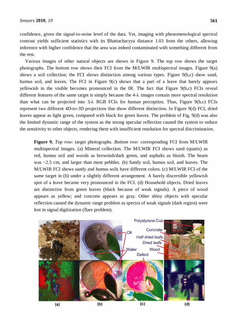
However, an example of a more challenging problem, which also underscores the usefulness of
laser spectral imaging is the case of drug pills shown in Figure 15. Figure 15(a) shows a conventional
visible image (photograph) of two common drug pills, both appeared white. The question is whether
there is any spectroscopic feature or difference between them, and what laser spectral imaging can
detect. Unlike the glucose problem in Section 6.2, in which the spectral signature is known and the
experiment was designed to search for it, there is no prior knowledge of the two pills spectroscopic
properties. The experiments were performed for the vis-near IR region, from 0.69 to 1.55 m. The
problem is that they appear to have very little spectroscopic characteristics in this spectral region, and
thus pose a more interesting test to laser multispectral imaging.
The 5 × 6 matrix of scattering coefficient rS ;; images for wavelength from 0.69 to 1.55 m
(vertical, column) and for polar scattering angle from 30 to 80 degree off incident (horizontal, row)
are shown in Figure 15(b). In principle, scattering images vs. azimuthal angle should have also been
measured; however, observation indicated that the azimuthal scattering was generally uniform except
Figure 14. Example of spectral images with features that allow strong discrimination
[27]. (a) Legitimate US currency (top left 4 images) vs. its color photocopy (bottom left 4
images). The false color images (FCI) right top and bottom are discriminated mainly on
the 830 nm spectral images. (b) Similar experiments on common marker dark blue ink vs.
FDC#1 blue. The two FCI’s show their spectral difference and detailed variation within
the large letters.
FDC #1 Blue
common marker
Regular Marker 635 nm 650 nm
690 nm 850 nm
(a) (b)
False color image
False color image
635 nm
Legitimate currency
650 nm
690 nm 830 nm
Color copy
635 nm 650 nm
690 nm 830 nm
Sensors 2010, 10
570
for some extreme locations with sharp edges or pointed depression and protrusion. It was decided that
these locations were not significant and errors from them were acceptable.
Conventionally, the spectral images of Figure 15(b), in which each pixel is a vector in 30-D space,
are processed with various image processing algorithms to enhance the features of interest if they are
known or expected. Alternatively, the images can be phenomenologically classified into clusters in
the 30-D space. Then three processed images with the most interest aspects can be combined for a
RGB FCI. In this case, there is a large amount of information in the 30 images; and the classification
can range from very fine to very coarse as desired. Not every piece of information is of interest
however. In fact, every single pixel is virtually unique in this 30-D space and can be statistically
discriminated from all others. The objective here is not to discriminate various pixels for the sake of
discrimination. It is only to compare the pills and see if there is meaningful spectroscopic information.
Therefore, the approach is not to interpret the images with phenomenological pattern recognition, but
with light scattering principles. For example, simple shadowing effect caused one pill to be spectrally
darker than the other. Pure phenomenological classification can claim this as a discriminating feature,
but clearly, it is not meaningful for this purpose.
The interpretation must deal with both angular and wavelength-dependence variations in the images,
which were far from uniform within the measurement uncertainty over the pill surfaces. Although
there was some evidence of spectral signature with long wavelength, 1.31 and 1.55 m, the amplitude
of these signals is only comparable to other variation that is caused by the surface geometrical or
morphological effect. As discussed in Section 6.3 above, there is a spectral effect on SI ΩΩS ˆ;ˆ of
Equation (9) that is unrelated to the spectroscopy of r; . In this particular case, it is the geometrical
effect associated with -dependence interference and diffraction. For a random surface, this often gives
rise to the speckle effect in high coherence case. Even for incoherent radiation, this effect exists, which
is the reason why a surface that is rough in the visible, can act like a mirror in the IR. Some aspect of
this effect has been studied and discussed in WMS imaging [22].
Figure 15. (a) A conventional visible photograph of two drug pills. (b) Scattering
coefficient images for wavelength from 0.69 from 1.55 m (vertical, column) and for
viewing angle from 30-80 degree (horizontal, row). (c) False color image of scattering
properties of the two pills, taking into account both angular and wavelength data.
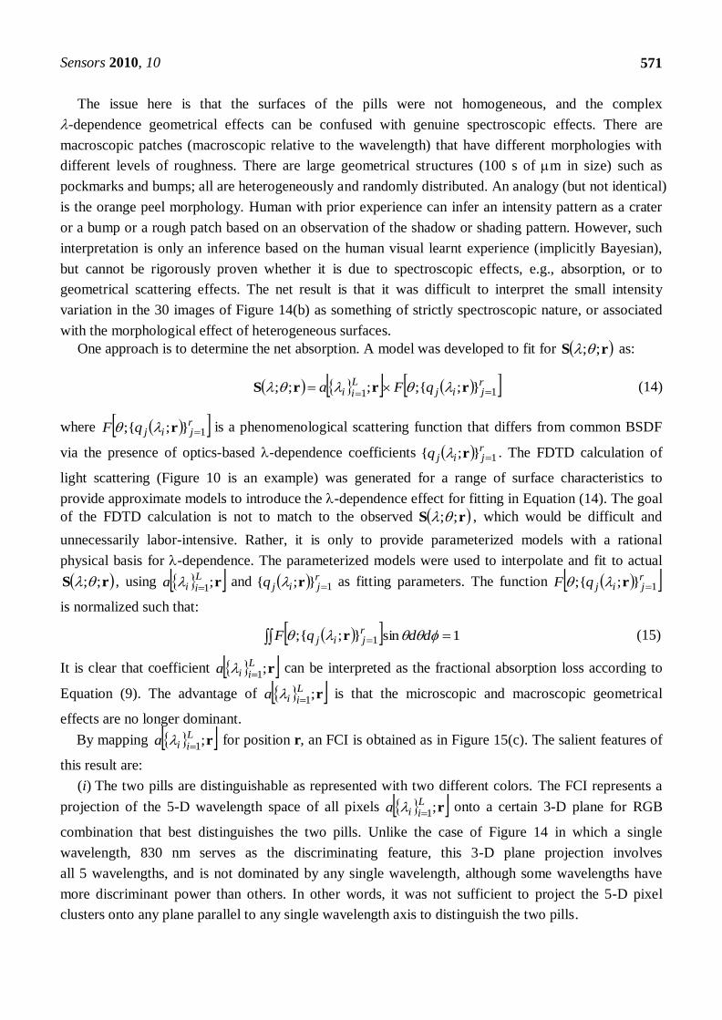
Sensors 2010, 10
571
The issue here is that the surfaces of the pills were not homogeneous, and the complex
-dependence geometrical effects can be confused with genuine spectroscopic effects. There are
macroscopic patches (macroscopic relative to the wavelength) that have different morphologies with
different levels of roughness. There are large geometrical structures (100 s of m in size) such as
pockmarks and bumps; all are heterogeneously and randomly distributed. An analogy (but not identical)
is the orange peel morphology. Human with prior experience can infer an intensity pattern as a crater
or a bump or a rough patch based on an observation of the shadow or shading pattern. However, such
interpretation is only an inference based on the human visual learnt experience (implicitly Bayesian),
but cannot be rigorously proven whether it is due to spectroscopic effects, e.g., absorption, or to
geometrical scattering effects. The net result is that it was difficult to interpret the small intensity
variation in the 30 images of Figure 14(b) as something of strictly spectroscopic nature, or associated
with the morphological effect of heterogeneous surfaces.
One approach is to determine the net absorption. A model was developed to fit for rS ;; as:
rjij
Lii qFa 11
};{;;;; rrrS (14)
where rjijqF 1};{; r is a phenomenological scattering function that differs from common BSDF
via the presence of optics-based -dependence coefficients rjijq 1};{ r . The FDTD calculation of
light scattering (Figure 10 is an example) was generated for a range of surface characteristics to
provide approximate models to introduce the -dependence effect for fitting in Equation (14). The goal
of the FDTD calculation is not to match to the observed rS ;; , which would be difficult and
unnecessarily labor-intensive. Rather, it is only to provide parameterized models with a rational
physical basis for -dependence. The parameterized models were used to interpolate and fit to actual
rS ;; , using r;1
Liia
and rjijq 1};{ r as fitting parameters. The function r
jijqF 1};{; r
is normalized such that:
1sin};{; 1 ddqF rjij r (15)
It is clear that coefficient r;1
Liia
can be interpreted as the fractional absorption loss according to
Equation (9). The advantage of r;1
Liia
is that the microscopic and macroscopic geometrical
effects are no longer dominant.
By mapping r;1
Liia
for position r, an FCI is obtained as in Figure 15(c). The salient features of
this result are:
(i) The two pills are distinguishable as represented with two different colors. The FCI represents a
projection of the 5-D wavelength space of all pixels r;1
Liia
onto a certain 3-D plane for RGB
combination that best distinguishes the two pills. Unlike the case of Figure 14 in which a single
wavelength, 830 nm serves as the discriminating feature, this 3-D plane projection involves
all 5 wavelengths, and is not dominated by any single wavelength, although some wavelengths have
more discriminant power than others. In other words, it was not sufficient to project the 5-D pixel
clusters onto any plane parallel to any single wavelength axis to distinguish the two pills.

Sensors 2010, 10
572
This simple result is highly deceptive for its apparent obviousness. If the pixels were segmented
phenomenologically in the 30-D space and projected into other arbitrary 3-D plane, there would be
pixels from both pills grouped together as being in the same category, and spatially adjacent pixels
could have been segregated into different categories. The result would have been two pills with
mixture of multi-colors pixels, but not necessarily distinguishable from each other except for the
overall shape. Here, the two pills are recognized as of slightly different spectroscopic property that is
independent of their morphological scattering property.
(ii) The dark spots in the FCI of each pill represent true spectral absorbance that is distinguishable
from their surroundings. The main discrimination features here are the l.31 and 1.55 m as mentioned
above. The dark spots were proved not to be results of some intensity variation associated with surface
texture variation. And likewise, the effect of surface coarse texture was also removed in the image. In
other words, without the dark spots, each pill would have appeared almost of a uniform color.
We hypothesize the dark spots as indicators of pharmaceutical ingredients. Note that their grain size
as well as spectral nature is clearly different for the two drug pills. Again, this result is also deceptive
for its simplicity. A purely data driven phenomenological classification would form a matrix of both
spectral and morphological spots, and it would be difficult to discern the pharmaceutical ingredient
particles from the surface bumps and troughs. It is also clear that there are some errors at the sharp
edges that had strong scattering and for which the model of Equation (15) was not valid, resulting in
wrong classification.
It should be note that the FCI image Figure 15(c) is not a direct construction from various linear
combinations of the rS ;; of Figure 15(b), but only represents a mapping of coefficient r;1
Liia
,
which is fundamentally of a different nature than the conventional scattered light intensity images in
Figure 15(b). This result shows the versatility of spectral imaging, which can be applied beyond the
original concept of scattered light mapping to generate secondary images (derived images) for relevant
information. The difference between the spectral imaging result in this section vs. that of Section 5 is
that the Section 5 images were obtained with much lower SNR, with lower laser power and at a
standoff distance. In compensation, the use of M/LWIR helped better spectroscopic discrimination for
those targets in Section 5. In this section, the vis-near-IR imaging of the drug pills enjoyed no such
natural spectroscopic contrast. On the other hand, the experiments had much higher SNR. This
illustrates the laser advantages of radiometric accuracy and dynamic range that allow the distinction of
small spectral difference, which could otherwise be difficult with the passive methods.
7. Results on WMS Imaging with Tunable MWIR Lasers
In the results of Section 5 and 6, multi-spectral imaging was applied for spectral discrimination of
various targets, but not for the identification of any target with prior spectroscopic knowledge, except
for the glucose detection. A multi-spectral imaging system can also perform spectroscopic
identification under appropriate condition. This section describes the use of a tunable MWIR laser
coupled into the same imaging system to performed WMS absorption imaging of CO gas. More details
can be found in [22]. The use of semiconductor-laser-based system for WMS methane gas detection
has been well developed and commercialized [33-35]. A fortuitous advantage in this case is the

Sensors 2010, 10
573
methane overtone absorption line at 1.651 m, which is within the range of affordable DFB lasers of
telecom technology.
In this experiment, the CO gas was confined to a tube as shown in the top left photograph of
Figure 16(a), owing to its toxicity. The transmitted beam was scattered off from a topographic target
and detected. The MWIR laser was tuned to the CO absorption line at 4.88693 m, and the 2nd
order
WMS measurement was performed. The 2nd
order WMS image was shown in the top right of
Figure 16(a). Since all other objects in the scene besides CO gas have very small 2nd
order derivatives
at this particular wavelength, they do not appear on the WMS image, and the result is specific to CO
gas detection and identification.
A concept for more practical application is illustrated in Figure 16(b). A synthetic image obtained
by digital fusion of a CCD camera image of the gas cell with the 2nd
order WMS image of CO is
shown in the bottom of Figure 16(a). The fusion was performed on a computer; however, the algorithm
can easily be implemented with a dedicated FPGA. More generally, a system with many
wavelengths can simultaneously detect different spectroscopic signatures and use color-coding to
show different species.
A point worth noting is that imaging also offers additional knowledge, as opposed to spectroscopic
sensing of a single point. Although most objects apart from CO gas have very small WMS signature, it
is nevertheless detectable above the noise level. This is not the system bias which is a non-zero
“baseline” that must be removed as a part of system calibration. In fact, wavelength-modulation
Figure 16. (a) Top left: a CCD visible image of the CO gas tube. Top right: the 2nd
order
wavelength modulation spectroscopy (WMS) image of the entire scene, measured at
the 4.88693 m, showing only the signature of CO absorption, since all other objects
have negligible 2nd
order WMS signals. Bottom: a synthetic image, obtained by digital
combination of the CCD visible image in top left with the 2nd
order WMS image in top
right. (b) Concept diagram of a combined passive and active imaging system that would
allow synthetic images such as the bottom of (a) [22].
(a) (b)

Sensors 2010, 10
574
imaging (WMI) is more general than WMS and not just for gas detection. The geometrical effects
discussed in Section 6 above also have WMI signature [22], which can obfuscate the spectroscopic
signature. Imaging allows spatial discrimination, which is the comparison of different points of the
scene to decide if the signal is from a background or something that is standout among other objects.
Together with multispectral capability, which allows measuring with different wavelengths to improve
the specificity with respect to a gas, the technique can overcome these issues to provide more accurate
spectroscopic imaging.
8. Conclusions
Multi-spectral laser imaging technique using semiconductor lasers was studied and demonstrated
for a variety of targets to evaluate the technique capability and potential applications. Semiconductor
lasers are significant with regard to potential practicality and affordability; however, they also warrant
considerations on system design and engineering. The basic system design, issues on engineering, and
measuring approaches are discussed with regard to the tradeoff between the staring imaging technique
and scanning imaging technique that is appropriate for low power such as semiconductor lasers.
Although the number of lasers and wavelengths are modest for the system studied, which included
a four M/LWIR-wavelength system and five vis-near-IR-wavelength system, the various results in
Sections 5–7 show the potential and capability of this technology. For a variety of targets, ranging
from common natural and man-made materials, the M/LWIR results demonstrated high multi-spectral
resolution to help discriminate complex targets. The issue of diffuse scattering in spectral imaging was
also discussed, with examples on glucose measurements and vis-near-IR imaging of drug pills. WMS
imaging for gas detection also show its compatibility with conventional spectroscopy.
Multispectral and hyperspectral imaging with passive techniques have been well developed for
numerous applications involving target spectral segmentation, discrimination, and identification. Yet,
the passive technique cannot avoid some uncertainty and ambiguity on the background radiation, as
well as a lack of strong signals in some cases. This is not an issue with laser spectral imaging, as the
laser light can be discriminated from the background. Furthermore, although this works involved only
elastic scattering imaging, the system design and analysis here are obviously relevant and applicable to
other laser spectroscopic techniques such as Raman, fluorescence, photoacoustic, or nonlinear optics.
As laser spectroscopic sensing is well proven of its value, it is natural to extend the laser spectroscopic
capability into the multi-spectral imaging domain that can offer the combined power and capability of
both techniques. This paper aims to contribute to the development of this trend.
Acknowledgements
Part of this work was sponsored by the US DARPA, and the US Department of Justice.
References and Notes
1. Infrared and Raman Spectroscopic Imaging; Salzer, R., Siesler, H.W., Eds.; Wiley-VCH:
Weinheim, Germany, 2009.

Sensors 2010, 10
575
2. Chang, C.I. Hyperspectral Imaging: Techniques for Spectral Detection and Classification;
Springer: Berlin, Germany, 2003.
3. Levenson, R.M.; Mansfield, J.R. Multispectral imaging in biology and medicine: Slices of life.
Cytometry A 2006, 69, 748–758.
4. Lidar—Range-Resolved Optical Remote Sensing of the Atmosphere; Weitkamp, C., Ed.; Springer:
Berlin, Germany, 2005.
5. Swim, C.; Vanderbeek, R.G.; Emge, D.; Wong, A. Overview of chem-bio sensing. Proc. SPIE
2006, 6218, 621802–621809.
6. Warren, R.E.; Vanderbeek, R.G.; Ahl, J.L. Detection and classification of atmospheric arerosols
using multi-wavelength LWIR LIDAR. Proc. SPIE 2009, 7304, doi:10.1117/12.818694.
7. Gimmestad, G.G.; Differential-Absorption Lidar for Ozone and Industrial Emissions.
In Lidar—Range-Resolved Optical Remote Sensing of the Atmosphere; Weitkamp, C., Ed.;
Springer: Berlin, Germany, 2005.
8. Weibring, P.; Smith, J.N.; Edner, H.; Svanberg, S. Development and testing of a frequency-agile
optical parametric oscillator system for differential absorption lidar. Rev. Sci. Instrum. 2003, 74,
4478–4492.
9. Prasad, C.R.; Kabro, P.; Mathur, S.L. Tunable IR differential absorption lidar for remote sensing
of chemicals. Proc. SPIE 1999, 3757, 87–97.
10. Weibring, P.; Abrahamsson, C.; Sjöholm, M.; Smith, J.N.; Edner, H.; Svanberg, S.
Multi-component chemical analysis of gas mixtures using a continuously tunable lidar system.
Appl. Phys. B: Lasers Opt. 2004, 79, 395–530.
11. Fujii, T.; Fukuchi, T.; Cao, N.; Nemoto, K.; Takeuchi, N.; Trace atmospheric SO2 measurement
by multiwavelength curve-fitting and wavelength-optimized dual differential absorption lidar.
Appl. Opt. 2002, 41, 524–531.
12. Velsko, S.P.; Ruggiero, A.J.; Hermann, M.R. Frequency-agile OPO-based transmitters for
multiwavelength DIAL. Proc. SPIE 1996, 2833, 144–154.
13. Pahlow, M.; Müller, D.; Tesche, M.; Eichler, H.; Feingold, G.; Eberhard, W.L.; Cheng, Y.
Retrieval of aerosol properties from combined multiwavelength lidar and sunphotometer
measurements. Appl. Opt. 2006, 45, 7429–7442.
14. Weibring, P.; Edner, H.; Svanberg, S. Versatile mobile lidar system for environmental monitoring.
Appl. Opt. 2003, 42, 3583–3594.
15. Müller, D.; Wandinger, U.; Althausen, D.; Fiebig, M. Comprehensive particle characterization
from three-wavelength raman-lidar observations: case study. Appl. Opt. 2001, 40, 4863–4869.
16. Althausen, D.; Müller, D.; Ansmann, A.; Wandinger, U.; Hube, H.; Clauder, E.; Zörner, S.
Scanning 6-wavelength 11-channel aerosol lidar. J. Atmos. Oceanic Technol. 2000, 17, 1469–1482.
17. Yabuki, M.; Kuze, H.; Kinjo, H; Takeuchi, N. Determination of vertical distributions of aerosol
optical parameters by use of multi-wavelength lidar data. Jpn. J. Appl. Phys. 2003, 42; 686–694.
18. Schliesser, A; Brehm, M.; Keilmann, F. Frequency-comb infrared spectrometer for rapid, remote
chemical sensing. Opt. Exp. 2005, 13, 9029–9038.
19. Andersen, J.F.; Busck, J.; Heiselberg, H. Pulsed Raman fiber laser and multispectral imaging in
three dimensions. Appl. Opt. 2006, 45, 6198–6204.

Sensors 2010, 10
576
20. Brown, D.M.; Shi, K.; Liu, Z.; Philbrick, C.R. Long-path supercontinuum absorption
spectroscopy for measurement of atmospheric constituents. Opt. Exp. 2008, 16, 8457–8471.
21. Vodopyanov, K. Sensing with mid-infrared frequency combs: a novel modality for ultrasensitive
detection of hazardous materials. Proc. SPIE 2009, 7304, doi:10.1117/12.820774.
22. Wang, Y.; Peng, C.; Zhang, H.; Le, H.Q. Wavelength modulation imaging with tunable
mid-infrared semiconductor laser: spectroscopic and geometrical effects. Opt. Exp. 2004, 12,
5243–5257.
23. Morbi, Z.; Ho, D.B.; Ren, H.W.; Le, H.Q.; Pei, S.S. Short-range remote spectral sensor using
mid-infrared semiconductor lasers with orthogonal code-division multiplexing approach. Opt. Eng.
2002, 41, 2321–2337.
24. Wang, Y.; Wang, Y.; Le, H.Q. Multi-spectral mid-infrared laser stand-off imaging. Opt. Exp.
2005, 13, 6572–6586.
25. Wang, Y.; Wang, Y.; Peng, C.; Zhang, H.; Seetheraman, A.; Le, H.Q. Concepts for scalable,
CDMA-networked, M/LWIR semiconductor laser standoff chemical detection system. Proc. SPIE
2004, 5617, 179–189.
26. Wang, Y.; Hu, B.; Le, H.Q. Laser multispectral polarimetric diffuse-scatter imaging. Proc. SPIE
2007, 6565, doi:10.1117/12.719247.
27. Wang, Y.; Wang, Y.; Le, H.Q. Multi-spectral imaging with mid-infrared semiconductor lasers.
Proc. SPIE 2005, 6062, doi:10.1117/12.643228.
28. Furstenberg, R.; Kendziora, C.A.; Stepnowski, J.; Stepnowski, S.V.; Rake, M.; Papantonakis,
M.R.; Nguyen, V.; Hubler, G.K.; McGill, R.A. Stand-off detection of trace explosives via
resonant infrared photothermal imaging. Appl. Phys. Lett. 2008, 93, 224103–224105.
29. Papantonakis, M.R.; Kendziora, C.A.; Furstenberg, R.; Stepnowski, S.V.; Rake, M.; Stepnowski,
J.; McGill, R.A. Stand-off detection of trace explosives by infrared photothermal imaging. Proc.
SPIE 2009, 7304, doi:10.1117/12.818752.
30. Gillespie, W.; Burd, J. Private communications, 2007.
31. Gillespie, W.; Le, H.Q. Unpublished data, 2007.
32. Guo, B.; Wang, Y.; Wang, Y.; Le, H.Q. Mid-infrared laser measurements of aqueous glucose.
J. Biomed. Opt. 2007, 12, 024005–024018.
33. Vujkovic-Cvijin, P.; Cooper, D.E.; van der Laan, J.E.; Warren, R.E.; Diode-laser-based lidars: the
next generation. Proc. SPIE 1999, 3758, 142–149.
34. Frish, M.B.; Wainner, R.T.; Green, B.D.; Laderer, M.C.; Allen, M.G. Standoff gas leak detectors
based on tunable diode laser absorption spectroscopy. Proc. SPIE 2005, 6010, 86–94.
35. Iseki, T.; Tai, H.; Kimura, K. A portable remote methane sensor using a tunable diode laser. Meas.
Sci. Technol. 2000, 11, 594–602.
36. Pattern Classification; Duda, R.O., Hart, P.E., Stork, D.G., Eds.; Wiley-Interscience: New York,
NY, USA, 2001.

Sensors 2010, 10
577
Appendix
A. System noise considerations for parallel and sequential measurements
This section considers the calculation of the laser power and image acquisition time for the parallel
and sequential methods as discussed in Section 2.3. For the sequential method, the signal-to-noise ratio
(SNR) of a single measurement (single pixel, single wavelength) is:
(A.1)
where P is the laser power, is the fraction of incident power that is returned as the signal, is the
measurement time, and NEP is the average noise equivalent power of the receiver. From
Equation (A.1), for a given desired SNR, the power required is:
(A.2)
From Equation (A.2), the measurement time required for each pixel for a given power is:
(A.3)
The total time required to complete an image with the sequential method is:
(A.4)
where subscript sequent denotes the sequential measurement method, Q is the number of spatial pixels,
L is the number of wavelengths, and t0 is the dead time when the system is busy, changing wavelength
or illuminating spot and does not perform a measurement.
For the parallel method, assume that P is simultaneously divided among all pixel-product QL,
Then, the average SNR of each pixel is:
(A.5)
and Equations (A.2) and (A.3) now become:
(A.6)
(A.7)
More generally, a hybrid approach can divide into block M × N, which means M sequential
measurements of N parallel-measured blocks. Then, the time is:
NEP
PSNR
NEPSNRP
1
21
NEPSNR
P
2
00
1NEPSNR
PtQLtQLTsequent
NEPQL
PSNR
NEPSNRQLP
1
paralTNEPSNRQLP
21
QL

Sensors 2010, 10
578
(A.8)
Comparing of Equation (A.4) and of Equation (A.7):
(A.9.a)
where, for simplicity is defined:
(A.9.b)
it appears that the sequential method allows faster (more efficient) image acquisition than the parallel
method as a function of increasing QL. Conversely, for the same total image acquisition time T, the
power required for the sequential method in Equation (A.2) is less than that for the parallel method in
Equation (A.6):
(A.10)
A more realistic noise model involves also the laser RIN (relative intensity noise). In this case, the
term NEP in the above equations is replaced by:
(A.11)
for the sequential term, and:
(A.12)
for the parallel term. They are simply the additive combination of receiver noise NEP and laser RIN.
For both, explicit frequency-dependence is shown to include realistic noise behaviors, which often
involve 1/f-component; and:
(A.13.a)
(A.13.b)
which represent the measurement frequencies of the serial and parallel methods, respectively.
Certainly, the laser intensity fluctuation effect, i.e., RIN can be reduced by dividing the received signal
with the monitored laser transmitted power. However, this can be sometimes impractical with respect
to system cost and complexity.
2
0, NEPSNRP
NtMT NM
sequentT paralT
QLT
T
paral
sequent
1
2
0
1/
NEPSNR
Pt
QLP
P
paral
sequent
1
22ss fRINPfNEPNEP
22 /QLFRINPFNEPNEP pp
222
21
ssss
fRINPfNEPSNR
Pf
222
2
/
1
QLFRINPFNEPQLSNR
PF
pppp

Sensors 2010, 10
579
Using Equations (A.11)–(A.13), Equation (A.9.a) becomes:
(A.14)
which asymptotically approaches to Equation (A.9.a) if laser RIN is negligible compared to the
receiver noise. Both Equations (A.13.a) and (A.13.b) entail a relationship, as fs and Fp appear on both
sides of the equations. This reflects the case when the noise power spectral density is not a flat white
spectrum, but may have f-dependency. It means that the desire SNR is achievable only if there is a
solution for (A.13.a) and (A.13.b).
B. Reflection from a thin-film on a dielectric substrate
This section derives Equations (10) and (11) in Section 6.2. Consider the case in Figure A.1, which
is a thin-film of material with dielectric function on a substrate with dielectric function .
The reflection coefficient of a plane wave with wave vector k and incident angle θinc can be
obtained by imposing the continuity boundary condition for the E and H field in the y-z plane at each
interface. For the TE mode, and for each region, air, film, substrate are:
Air: ; (A.15.a)
Film:
(A.15.b)
22
22
/
1
QLFRINPFNEP
fRINPfNEP
QLT
T
pp
ss
paral
sequent
f s
yE zH
reeeEE
xikxiktziy
aa1
0
reikeike
k
iEH
xika
xika
tziz
aa1
0
0
2
10
c
ceeeEE
xikxiktziy
ff
2
1
0
0
c
ceikeike
k
iEH
xikf
xikf
tziz
ff
Figure A.1. Reflectance from a thin-film layer on a dielectric substrate.
inc
d
k;r
inc2
0 sin ff kk
inc0 cos kka
inc0 sin k
inc2
0 sin ss kk

Sensors 2010, 10
580
Substrate: ;
(A.15.c)
where k0 ≡ 2π/λ, is the magnetic permeability, which is the same for all layer in this case, is the
light frequency, and other quantities are defined in Figure A.1. Two relevant coefficients are reflection
r in Equation (A.15.a) and transmission t in Equation (A.15.c); coefficients c1 and c2 in
Equation (A.15.c) are simply some values to be solved by imposing the boundary condition.
It is convenient to put Equations (A.15.a, b, c) in the matrix form, and drop term that is
common to all; then the continuity of and at each interface gives:
Air-film: (A.16.a)
Film-substrate: (A.16.b)
Eliminating coefficients c1 and c2 in both Equations (A.16.a and b) yields:
(A.17)
which can be solved to give:
(A.18.a)
(A.18.b)
where subscript TE indicates transverse electric. A similar result can be obtained for the TM mode:
(A.19)
which yields:
(A.20.a)
00
teeeEE
dxikdxiktziy
ss
00
0t
eikeikek
iEH
dxiks
dxiks
tziz
ss
tzieE 0
yE zH
2
1
00
11111
c
c
ikikrikikHki
E
ffaaxz
y
0
11
2
1
0
t
ikikc
c
eikeik
ee
Hki
E
ssdik
fdik
f
dikdik
dxz
y
ff
ff
0
111111111
t
ikikeikeik
ee
ikikikikr ssdik
fdik
f
dikdik
ffaaff
ff
sffa
idksffa
sffaidk
sffa
kkkkekkkk
kkkkekkkkr
f
f
2
2
TE ;k
sffa
idksffa
idkfa
kkkkekkkk
ekkt
f
f
2TE
4;k
0
11
0
01
111
0
01111
1
1
t
ikikeikeik
ee
ikikikikr
sss
fdikf
dikf
dikdik
fffaa
ff
ff
sffsfaf
idksffsfaf
sffsfafidk
sffsfaf
kkkkekkkk
kkkkekkkkr
f
f
2
2
TM ;k

Sensors 2010, 10
581
(A.20.b)
These results are used to plot Figure 13(e,f).
In the glucose experiments described in Section 6.2, the beam is not a plane wave, but a focused
beam. Thus, the beam can be expressed as a linear superposition of plane waves:
(A.21)
Each k component of Equation (A.21) contributes a reflection wave with amplitude:
(A.22)
where is given in Equation (A.18.a) or (A.20.a), depending on the polarization. The reflected
beam is a coherent sum of all reflected waves of Equation (A.22):
(A.23)
where , where , are the incident wave vector components in the y–z
plane. Since the beam has low NA focusing, with little transverse spatial component, one can
approximate as a constant , which can be taken out of the integral. Then the collected
power of the scattered beam is:
(A.24)
where is the receiver collection efficiency for beam in the viewing (receiving) angle , and
the integration is over the receiver angular aperture. If the receive responsivity is uniform over its field
of view, is simply = 1.
It should be noted that Equation (A.24) has general validity for diffuse scattering and is not limited
to that of Figure (A.1); and it was used for the FDTD computer simulation of scattering from a rough
surface as illustrated in Figure 10, except that coefficient is not that of Equations (A.18.a)
or (A.20.a) but represents the backscattering amplitude.
C. Detection of small contamination in elastic diffuse scattering:
Consider the case of scattering illustrated in Figure 11(b), but with the generalization for any
solvent with a small contamination. Let the film have a known dielectric function εf(λ), which is altered
to become εf(λ;CX) because of some contaminant X, and CX is its concentration. It is expected that
is small, such as ~10
−3 for glucose in Section 6.2 and even smaller in other
cases. The question is what is the physical basis for the contamination to be detected and quantified via
elastic scattering? In other words, how does CX manifest itself in the scattered light, and how does one
detect and quantify CX.
sffsfaf
idksffsfaf
idkfsfa
kkkkekkkk
ekkt
f
f
2TM
4;k
kkrrkk deeAE ii
kkk
ieAr ;
k;r
kkkr
rkk deeArEii refl;refl
zyak reflk y z
rk reflie
rk 0ie
2
apertureReceiver
;ˆˆˆ kkkΩΩΩk deArdHRS i
SSTS
SH Ω̂ SΩ̂
SH Ω̂
k;r
fff C /; X

Sensors 2010, 10
582
One can generally assume that the scattered electric field amplitude
is an unknown but
deterministic function of εf(λ;CX) and substrate dielectric function εs(λ). The scattered electric field
can be expanded with the first-order Taylor’s series:
(A.25)
where , and is the specific dielectric function per unit of substance concentration,
and is a substitution factor to account for the displacement of solvent molecules by those of
substance X. It should be noted that the model of Equation (A.25) is generic and not limited to the
configuration in Figure 11(b). The detected scattered field is a sum of all those in Equation (A.25), and
the total collected scattered intensity S is:
(A.26.a)
where: (A.26.b)
Applying Equation (A.26.b) in Equation (A.26.a), and keep the 1st order of CX, and furthermore,
split into its Re and Im component, then S consists of a background term without CX and a
term with CX:
(A.27)
where . For the derivative spectrum in the manner of WMS, the 1st order is:
(A.28.a)
where: (A.28.b)
Also: (A.28.c)
In light of Equations (A.28), any CX -dependent result in Figure 13 can be interpreted as a linear
combination of various terms in (A.28.a) column vector. The following are can be inferred:
(i) It is desirable that the term of Equation (A.28.c) does not have spectral features that
mask those of , , , and of Equation (A.28.a). For the
glucose experiments in Section 6.2, neither water nor the substrate has sharp features in the 9–10 m
range. and contribute at most a gradual linear baseline, which does not overwhelm
SE
X;,; CfsS E
XXX~0;,;;,; ε
εCC
f
SfsSfsS
EEE
f XX ˆ~X̂
;;,;2
X UCS fs
ff
SS
εεCd
εεCd
0XX0
;XX;
~~ UUk
EkEU
kk
X~
fffs εεCSCS
*
X
*
XX0X Im~ImRe~Re2;,;U
UU
U
200 US
;~Im~Re~Im~Re2;,; XX
XXX0
X
b
ad
dbd
da
d
εd
d
εdεεC
d
dSCS
d
dfs
kEkE
UU kk ddiba fsS
ffsS
f
,;,; *';;
*
d
dS
d
dSSS
d
d
d
dS f
f
s
sfs
,;0
X~ε
ddS /0
X~Reε X
~Imε dεd /~Re X dεd /~Im X
dd s / dd f /

Sensors 2010, 10
583
and . It is obviously futile to detect the signature of contaminant X over a
spectral range in which the solvent and/or a substrate have the same or similar spectral signature.
(ii) It is desirable that coefficients a(), b(), a’(), b’() be as large as possible. In Equation
(A.28.b), the magnitude of a() and b() depends on two terms. Normalized to incident laser power,
the crucial term determining the coefficient magnitude is:
(A.29)
This term entails that it is most desirable for the scattered field to be sensitive to the film dielectric
constant. This is also intuitively self-explanatory, since the measurement aims to detect very small
modification to the film εf(λ), hence the scattered field has to be insensitive to this quantity to detect a
small change.
(iii) With respect to the problem of quantification, CX cannot be determined independently unless
the coefficients are known. A desirable circumstance is that a’), b’) are negligible as discussed
in Section 6.3. Suppose there are L ≥ 2 wavelengths for measurement, then linear regression can be
used to infer the CX and coefficient products from the second-term of the right hand side of
Equation (A.28.a):
(A.30)
There are additional possible strategies to isolate the coefficients from CX, for example, the
coefficients also appear in the term of Equation (A.28.c), and a similar equation
can be obtained:
(A.31)
provided that the wavelength set 1’, 2’,… M’ is such that Equation (A.30) is negligible and so are
other terms in Equation (A.28.c). In essence, Equation (A.31) is to use the film εf(λ) as the calibration
material to determine a and b, which then can be used subsequently to infer CX.
© 2010 by the authors; licensee Molecular Diversity Preservation International, Basel, Switzerland.
This article is an open-access article distributed under the terms and conditions of the Creative
Commons Attribution license (http://creativecommons.org/licenses/by/3.0/).
dεd /~Re X dεd /~Im X
kE
kE
k
k
d
d
fsS
fsSf
,;
,;
;
';
ddS
ddS
ddS
bC
aC
εε
εε
εε
LLL /
/
/
'~Im'~Re
'~Im'~Re
'~Im'~Re
22
1
X
X
XX
2X2X
1X1X
ddS ff //
ddS
ddS
ddS
b
a
dddd
dddd
dddd
MMfMf
ff
ff
/'
/'
/'
/'Im/'Re
/'Im/'Re
/'Im/'Re
22
1
22
11