Embed Size (px)
Citation preview
EFFECTS OF WATER ON THE STRESS
CORROSION CRACKING OF CARBON
STEEL IN ETHANOLIC MEDIA
Fortunate Moyo
A research report submitted to the Faculty of Engineering and the Built
Environment, University of the Witwatersrand, Johannesburg, in partial
fulfilment of the requirements for the degree of Master of Science in
Engineering
Johannesburg, 2013

Page i
DECLARATION
I declare that this research report is my own unaided work. It is being submitted to
the degree of Master of Science in Engineering to the University of the
Witwatersrand, Johannesburg. It has not been submitted before for any other
degree or examination in any other University.
Fortunate Moyo
5th day of February 2013

Page ii
ABSTRACT
In this study, the effect of water on the stress corrosion cracking (SCC) of
ASTM 516 in ethanol was investigated. Ethanol is hygroscopic in nature and its
water content can increase rapidly when exposed to humid conditions. The
presence of water in ethanol is likely to increase ethanol’s oxygen content which
is the major instigator of SCC.
In order to have an insight into the SCC susceptibility of carbon steel in ethanol-
water solutions, the corrosion behaviour of the steel in these solutions was first
evaluated. Carbon steel specimens in ethanol solutions with water exhibited
various extents of localised corrosion, which increased in severity with increase in
water content from 1 to 5 vol%. The occurrence of localised attack suggested that
the presence of water promoted the formation of surface films; a condition
suitable for SCC. Carbon steel specimens subjected to slow strain rate tests,
however, exhibited ductile fractures indicating that the presence of up to 5vol%
water did not induce SCC of carbon steel in ethanol.

Page iii
To my parents
Kendu and Saziso Moyo

Page iv
ACKNOWLEDGEMENTS
The support of the DST/NRF Centre of Excellence in Strong Materials (CoE-SM)
towards this research is hereby acknowledged. I would also like to acknowledge
the financial aid contributed by the University of Witwatersrand Postgraduate
Merit Award.
I am grateful for the support of my supervisor, Josias Van Der Merwe, for his
patience and insightful mentorship. My profound gratitude goes to the technical
staff of the School of Chemical and Metallurgical Engineering especially
Shadrack, Theo, Rhod, Phatu, Bruce and Doctor for their invaluable assistance.
Great thanks to my fellow Masters students who made the year of my study
enjoyable.
Lastly, but not least, I wish to thank and acknowledge the support of my family
especially my sister Sanelisiwe.

Page v
CONTENTS
DECLARATION………………………………………………………………….i
ABSTRACT………………………………………………………………………ii
DEDICATION…………………………………………………………………..iii
ACKNOWLEDGEMENTS…………………………….………………………iv
CONTENTS ……………...………………………………………………………v
LIST OF FIGURES…………………………………………………………..…ix
LIST OF TABLES……………………………………………………………....xi
LIST OF SYMBOLS………………………………………………………...…xii
CHAPTER ONE: INTRODUCTION…………………………………………..1
1.1 Motivation…………………………………………………………………..1
1.2 Objectives…………………………………………………………………...3
1.3 Hypothesis…………………………………………………………………..3
1.4 Delimitations of the study…………………………………………………..4
1.5 Technical Approach…………………………………………………………4
CHAPTER TWO: LITERATURE REVIEW………………………………….5
2.1 Introduction…………………………………………………………………5
2.2 Ethanol………………………………………………………………………5
2.2.1 Production of ethanol……………………………………………………..6
2.2.2 Chemical properties of ethanol……………………………………………7
Ethanol and water…………………………………………………………….7
Ethanol and oxygen…………………………………………………………..8
2.3 Corrosion reactions…………………………………………………………8
Charge transfer control……………………………………………………….9
Diffusion control…………………………………………………………….10

Page vi
Mixed control………………………………………………………………..10
2.4 Stress corrosion cracking…………………………………………………..11
2.4.1 Definition of SCC………………………………………………………..11
2.4.2 Mechanisms of SCC……………………………………………………..13
Film rupture-Metal dissolution mechanism…………………………………13
Stress-sorption mechanism………………………………………………….14
Electrochemical mechanism………………………………………………...14
2.4.3 Crack morphology of SCC……………………………………………...15
2.4.4 SCC of carbon steel in ethanol environments…………………………...16
2.5 Monitoring corrosion processes…………………………………………...18
2.5.1 Linear polarisation resistance……………………………………………19
2.5.2 Electrochemical impedance spectroscopy……………………………….20
The Nyquist plot…………………………………………………………….21
The Bode plots………………………………………………………………22
CHAPTER THREE: EXPERIMENTAL METHODS……………………….24
3.1 Introduction………………………………………………………………..24
3.2 Materials used……………………………………………………………...24
3.3 Electrochemical measurements……………………………………………24
3.3.1 Apparatus………………………………………………………………...25
3.3.2 Sample preparation………………………………………………………26
3.3.3 Procedures……………………………………………………………….27
Linear polarisation resistance……………………………………………….27
Electrochemical impedance…………………………………………………27
3.3.4 Repeatability of the potentiostat……………………………………..…29
3.4 Slow strain rate test………………………………………………………..30
3.4.1 Apparatus………………………………………………………………..30
3.4.2 Sample preparation………………………………………………………32
3.4.3 Procedures……………………………………………………………….33
Calibration of the stepper motor…………………………………………….33
SSRT………………………………………………………………………...33
3.5 Solution characterisation…………………………………………………..34
Page vii
3.5.1 Apparatus………………………………………………………………...34
3.5.2 Procedures……………………………………………………………….34
Water content………………………………………………………………..34
Conductivity and dissolved oxygen…………………………………………35
Acidity………………………………………………………………………35
3.6 Metallographic analysis……………………………………………………35
3.6.1 Apparatus………………………………………………………………...35
3.6.2 Procedures……………………………………………………………….36
3.7 Immersion test……………………………………………………………..36
3.7.1 Procedures……………………………………………………………….36
CHAPTER FOUR: RESULTS AND DISCUSSION
CORROSION CHARACTERISATION…………………………….……….38
4.1 Introduction………………………………………………………………..38
4.2 Solution characterisation…………………………………………………..38
4.2.1 Conductivity……………………………………………………………..38
4.2.2 Dissolved oxygen………………………………………………………..43
4.2.3 Acidity…………………………………………………………………...46
4.3 Passivation tendencies……………………………………………………..50
4.4 Corrosion mechanism……………………………………………………...53
4.5 Corrosion rates……………………………………………………………..57
CHAPTER FIVE: RESULTS AND DISCUSSION
FAILURE ANALYSIS…………………………………………………………61
5.1 Introduction………………………………………………………………..61
5.2 Characterisation of the carbon steel……………………………………….61
5.3 SCC susceptibility…………………………………………………………62
5.4 Surface examination……………………………………………………….68
CHAPTER SIX: CONCLUSIONS……………………………………………72

Page viii
REFERENCES…………………………………………………………………74
APPENDICES…………………………………………………………………..80
Appendix A: Water contents estimations…….………………………………..80
Appendix B: SSRT…………….………………………………………………83
Page ix
LIST OF FIGURES
Figure 2.1: Flowchart showing the steps in the production of ethanol……………6
Figure 2.2: The factors that contribute to SCC…………………………………..11
Figure 2.3: A typical polarisation curve for an active/passive alloy……………..12
Figure 2.4: The effect of SCC on the load carrying thickness…………………...13
Figure 2.5: SCC in brass exposed to ammonia……………...…………………...15
Figure 2.6 Schematic presentation of SCC cracking modes..…………………....16
Figure 2.7: SCC in steel equipment used in fuel ethanol………………………...17
Figure 2.8: Crack velocity and water content in fuel ethanol……………………18
Figure 2.9: A linear polarisation plot………………………………………….....19
Figure 2.10: A typical Nyquist plot……………………………………………...22
Figure 2.11: Typical Bode plots…………………………………………………23
Figure 2.12: A typical equivalent circuit…………………………………………23
Figure 3.1: Arrangement of the Autolab, water bath and Faraday cage…………25
Figure 3.2: The corrosion cell inside the Faraday cage………………………….26
Figure 3.3: Equivalent circuits used to evaluate EIS data……………………….28
Figure 3.4: The tensile testing machine for SSRT without the corrosion cell…...31
Figure 3.5: The corrosion cell used in the tensile test……………………………32
Figure 3.6: Dimensions for SSRT specimens……………………………………32
Figure 3.7: The arrangement for measuring pHe………………………………...34
Figure 3.8: Dimensions for the immersion coupons…………………………..…36
Figure 4.1: Conductivity of ethanol-water solutions before immersion………....39
Figure 4.2: Solution resistance measured by EIS………………………………...41
Figure 4.3: Conductivity after 72 hours of immersion…...………………………42
Figure 4.4: Variation of dissolved oxygen with time and water content………...44
Figure 4.5: Variation of pHe with water content………………………………...48
Figure 4.6: Change in water content after 90 days of immersion……………….49
Figure 4.7: Evolution of OCP with time for different ethanol-water solutions….51
Figure 4.8: Double layer capacitance as a function of water content……………52
Figure 4.9: Nyquist and Bode plots for the carbon steel specimens……………..54
Figure 4.10: Micrographs of the carbon steel after 72 hours of immersion……...56
Page x
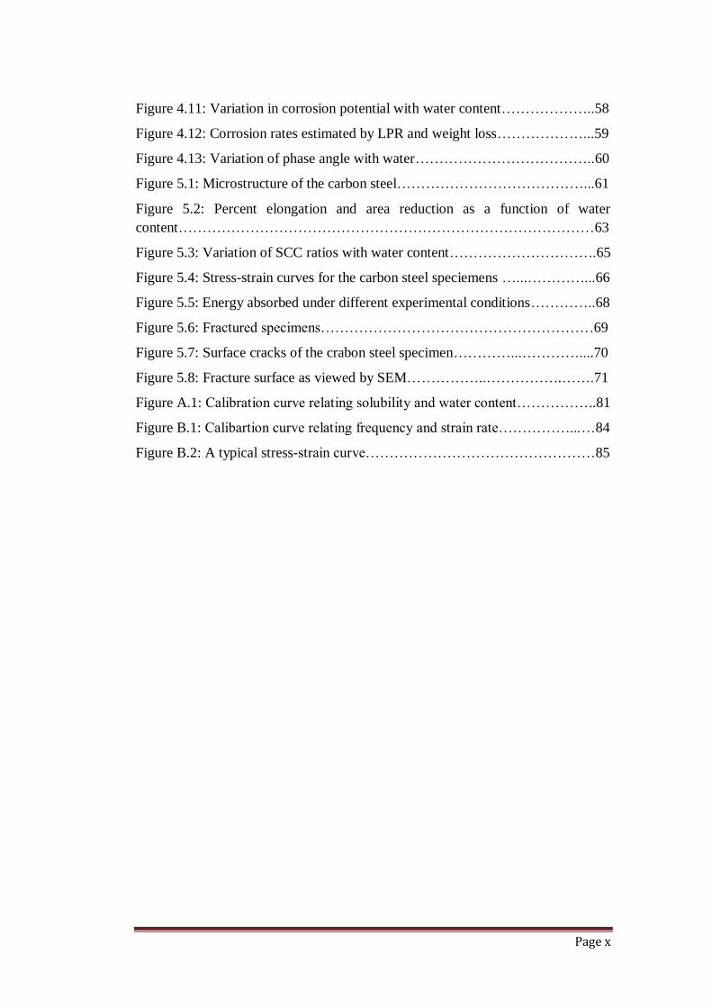
Figure 4.11: Variation in corrosion potential with water content………………..58
Figure 4.12: Corrosion rates estimated by LPR and weight loss………………...59
Figure 4.13: Variation of phase angle with water………………………………..60
Figure 5.1: Microstructure of the carbon steel…………………………………...61
Figure 5.2: Percent elongation and area reduction as a function of water
content……………………………………………………………………………63
Figure 5.3: Variation of SCC ratios with water content………………………….65
Figure 5.4: Stress-strain curves for the carbon steel speciemens …...…………...66
Figure 5.5: Energy absorbed under different experimental conditions…………..68
Figure 5.6: Fractured specimens…………………………………………………69
Figure 5.7: Surface cracks of the crabon steel specimen…………...…………....70
Figure 5.8: Fracture surface as viewed by SEM……………..…………….…….71
Figure A.1: Calibration curve relating solubility and water content……………..81
Figure B.1: Calibartion curve relating frequency and strain rate……………...…84
Figure B.2: A typical stress-strain curve…………………………………………85
Page xi
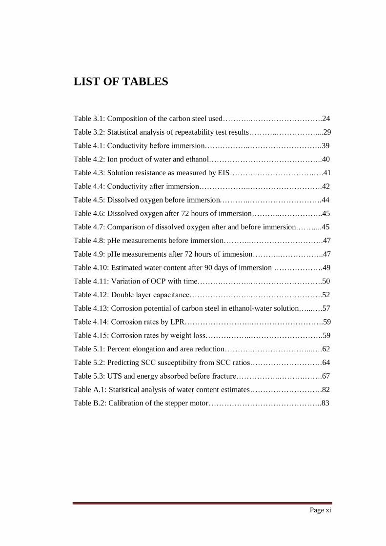
LIST OF TABLES
Table 3.1: Composition of the carbon steel used………..……………………….24
Table 3.2: Statistical analysis of repeatability test results………..……………....29
Table 4.1: Conductivity before immersion…….………..……………………….39
Table 4.2: Ion product of water and ethanol……………………………………..40
Table 4.3: Solution resistance as measured by EIS………..………………….….41
Table 4.4: Conductivity after immersion………………..……………………….42
Table 4.5: Dissolved oxygen before immersion.………..……………………….44
Table 4.6: Dissolved oxygen after 72 hours of immersion………..……………..45
Table 4.7: Comparison of dissolved oxygen after and before immersion.……....45
Table 4.8: pHe measurements before immersion………..……………………….47
Table 4.9: pHe measurements after 72 hours of immesion………..……………..47
Table 4.10: Estimated water content after 90 days of immersion ……………….49
Table 4.11: Variation of OCP with time……….………..……………………….50
Table 4.12: Double layer capacitance…………….……..……………………….52
Table 4.13: Corrosion potential of carbon steel in ethanol-water solution…...….57
Table 4.14: Corrosion rates by LPR……………………..……………………….59
Table 4.15: Corrosion rates by weight loss……….……..……………………….59
Table 5.1: Percent elongation and area reduction………..…………………...….62
Table 5.2: Predicting SCC susceptibilty from SCC ratios……………………….64
Table 5.3: UTS and energy absorbed before fracture……………..……….…….67
Table A.1: Statistical analysis of water content estimates……………………….82
Table B.2: Calibration of the stepper motor……………………………………..83

Page xii
LIST OF SYMBOLS
A Area [mm2]
γ Surface energy
pH Negative logarithm of hydrogen ions in aqueous solutions
pHe Negative logarithm of hydrogen ions in ethanol solutions
pKa Negative logarithm of the acid dissociation constant
Ks Ionic product
k Conductivity [µS/cm]
I Current [A]
E Voltage [V]
ΔI Change in current [A]
ΔE Change in potential [V]
iR Ohmic drop [V]
Ecorr Free corrosion potential [V]
Icorr Corrosion current density [A/m2]
βa Anodic Tafel constant [V/dec]
βc Cathodic Tafel constant [V/dec]
η Overpotential [V]
ηA Activation polarisation [V]
ηC Concentration [V]
D Diffusion coefficient [cm2/s]
dC Concentration gradient [mol/cm3]
dx The Nerst diffusion layer [cm]
Rp Polarisation resistance [Ωm2]
RΩ Ohmic resistance [Ω]
Page xiii
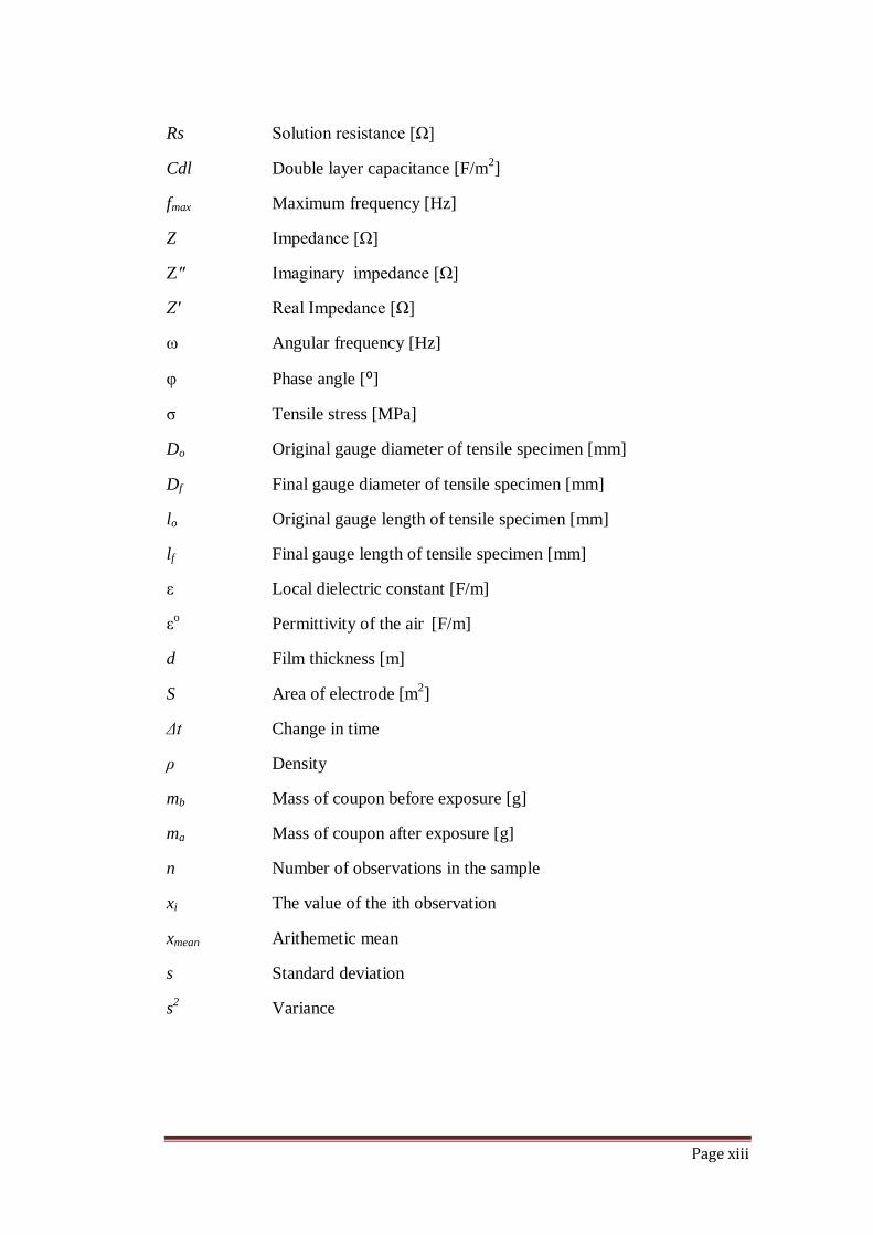
Rs Solution resistance [Ω]
Cdl Double layer capacitance [F/m2]
fmax Maximum frequency [Hz]
Z Impedance [Ω]
Z″ Imaginary impedance [Ω]
Z′ Real Impedance [Ω]
ω Angular frequency [Hz]
φ Phase angle [⁰]
σ Tensile stress [MPa]
Do Original gauge diameter of tensile specimen [mm]
Df Final gauge diameter of tensile specimen [mm]
lo Original gauge length of tensile specimen [mm]
lf Final gauge length of tensile specimen [mm]
ε Local dielectric constant [F/m]
εo Permittivity of the air
[F/m]
d Film thickness [m]
S Area of electrode [m2]
Δt Change in time
ρ Density
mb Mass of coupon before exposure [g]
ma Mass of coupon after exposure [g]
n Number of observations in the sample
xi The value of the ith observation
xmean Arithemetic mean
s Standard deviation
s2 Variance
Page xiv
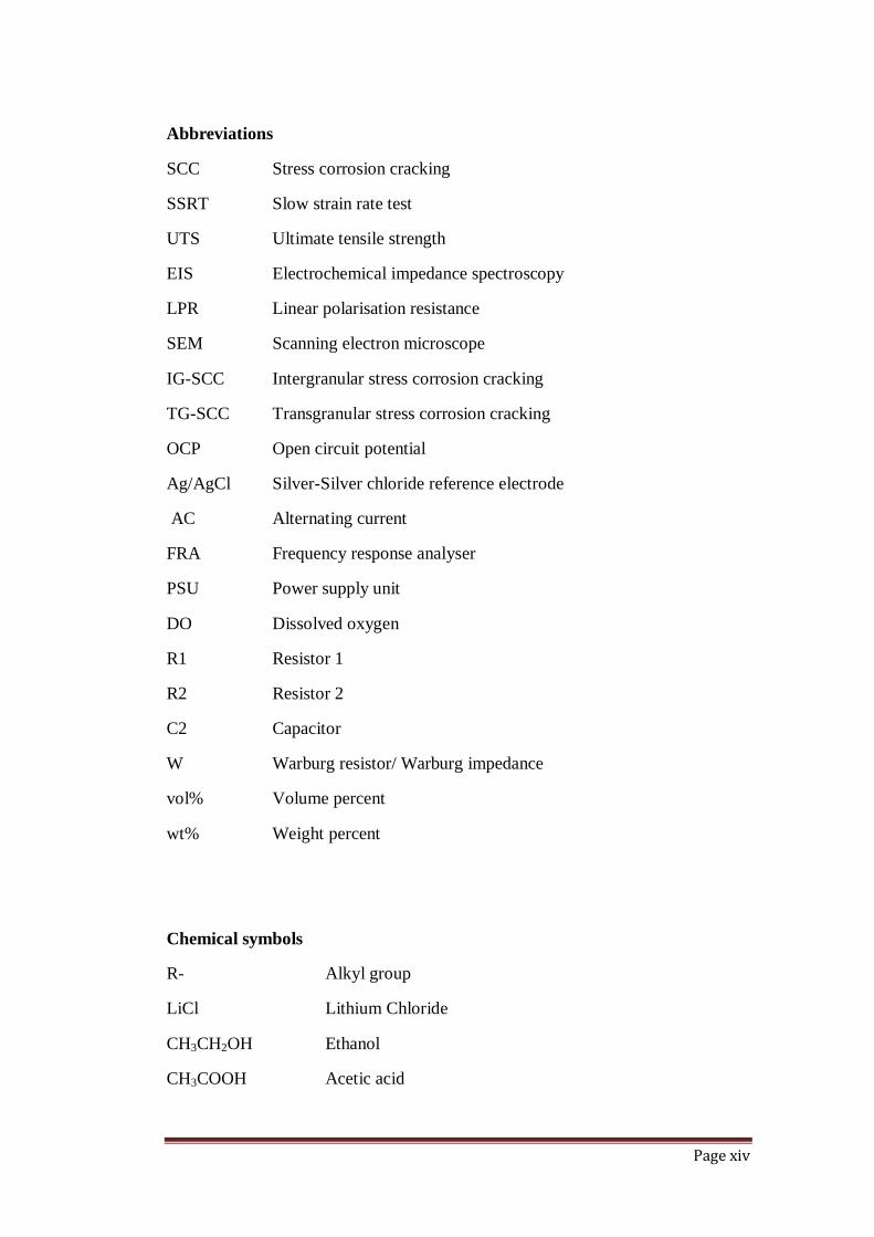
Abbreviations
SCC Stress corrosion cracking
SSRT Slow strain rate test
UTS Ultimate tensile strength
EIS Electrochemical impedance spectroscopy
LPR Linear polarisation resistance
SEM Scanning electron microscope
IG-SCC Intergranular stress corrosion cracking
TG-SCC Transgranular stress corrosion cracking
OCP Open circuit potential
Ag/AgCl Silver-Silver chloride reference electrode
AC Alternating current
FRA Frequency response analyser
PSU Power supply unit
DO Dissolved oxygen
R1 Resistor 1
R2 Resistor 2
C2 Capacitor
W Warburg resistor/ Warburg impedance
vol% Volume percent
wt% Weight percent
Chemical symbols
R- Alkyl group
LiCl Lithium Chloride
CH3CH2OH Ethanol
CH3COOH Acetic acid

Page xv
Acronyms
UN-Energy United Nations Energy
ORNL Oak Ridge National Laboratory
API American Petroleum Institute
US United States
ACE Associated Chemical Enterprise
ASTM American Society for Testing and Materials International
NACE National Association of Corrosion Engineers International
ASM American Society for Materials
NPL National Physical Laboratory
REM Renewable Energy Magazine

Page 1
CHAPTER ONE
INTRODUCTION
1.1 Motivation
Most of the world’s energy consumption originates from fossil sources such as
coal, gas and oil. The concern surrounding the sustainability of these fuels has
raised contentious debates and has increased the demand for alternative fuels. In
addition to the depletion of their sources and their ever fluctuating prices, these
fuels are associated with huge emissions of hydrocarbons and carbon dioxide,
both of which are major contributors to global warming (Fergusson, 2001).
Biomass products such as bioethanol and biodiesel have been explored as
potential alternative fuels to those that are petroleum-derived. Of these, bioethanol
has gained significant interest because it can be used in all existing petrol engines
without modifications. Popular ethanol blend fuel brands include E10 and E85
which contain 10 and 85% ethanol respectively. On the 23rd
August 2012, South
Africa’s Department of Energy published regulations regarding mandatory
blending of fuels with bioethanol (Herald, 2012); after announcing plans to invest
R2 billion in an ethanol plant earlier in the year (Roelf, 2012). The move is in line
with the world’s trends towards ‘greener’ and less costly fuels.
The move to introduce this regulation is not only aimed at decreasing South
Africa’s carbon footprint but is also set to reduce her reliance on imported fuels.
For a country reeling under very high unemployment rates, at 29.8% as of the first
week of October 2011, (Statssa, 2012) the increase in ethanol production could
also lead to increased job creation. RFA (2012) reported that in the USA, ethanol
production was responsible for 90 200 direct jobs in 2011 alone. In addition,
ethanol production could increase household income for the farming rural folk
Page 2
and reduce the high rural-to-urban migration currently being experienced in the
country (Statssa, 2012).
The world’s leading consumers of bioethanol are Brazil, USA and Sweden, with
100% of Brazil’s fuelling stations providing ethanol blended fuels
(UN Energy, 2011). According to a report by ORNL (2008), these countries and
others have reported occurrences of SCC of carbon steels exposed to ethanol
fuels. Carbon steel is a very versatile form of steel. It has a wide range of
engineering applications and its relatively low cost makes it an ideal material for
projects requiring a lot of steel. In Brazil, carbon steels are commonly used in
ethanol plants (Osterman, 2012) while in the USA, user terminals’ storage tanks,
pipes, loading/unloading racks are usually made of carbon steel (Beavers et al.,
2008).
During their service lives, these structures are subjected to different forms of
stress. Buried pipes, for example, may be subjected to subsidence of the ground
while suspended pipes may experience stresses from misalignment during
assembly or simply as a result of unevenly distributed dead loads. In addition,
welding and machining of components often leaves them with high residual
stresses, creating an ideal environment for SCC initiation (Scheel, 2010).
Extensive work has been done on the SCC of carbon steel in ammonia and
carbonated solutions, yet little is understood on this phenomenon in ethanol. In the
1990s, the American Petroleum Institute (API) pioneered research into the SCC of
carbon steel in ethanol and ethanol-blended fuels. Since then, there has been a
growing interest in the phenomenon (Kane et al., 2004; Sridhar, 2006; Lou et al.,
2009; Lou & Singh, 2011) with most work focused on the environmental factors
that may affect SCC behaviour of carbon steel in ethanol and ethanol blended
fuels. These studies recognised that the presence of certain impurities in ethanol
affected its aggressiveness and therefore its ability to support SCC. One of these
impurities is water.
Ethanol is hygroscopic in nature (Codd et al., 1972; Sridhar, 2006). If exposed to
humid conditions, its water content will increase radically. During the production
Page 3
of ethanol, water enters the ethanol stream as water vapour in the hot product.
This, coupled with the fact that ethanol forms an azeotrope with water, it is almost
impossible for an ethanol stream to have no water. Despite this, little analytical
attention has been paid to the effect of water on the SCC behaviour of carbon steel
in ethanol. Most studies have been based on high salt concentrations, yet in reality
ethanol has very low salt impurities (Lou & Singh, 2011). It is therefore probable
that at any given moment, a stream of ethanol would have a more significant
concentration of water than salts.
In anticipation of high ethanol production, it is necessary to recommend ways to
minimize SCC in carbon steels in contact with ethanol. The challenge is to
understand the mechanism of degradation of carbon steel in ethanol-water
mixtures so as to be able to predict the threshold water concentration for SCC and
hence prevent this insidious form of corrosion.
1.2 Objectives
The objectives of this research are;
1) To study the corrosion characteristics of carbon steel in mixtures of
ethanol and water.
2) To establish if ethanol-water mixtures can support SCC and hence
determine the threshold water concentration, in the absence of aggressive
salts, that can support SCC.
3) To ascertain if, in the absence of oxygen and ambient humidity, there is a
change in the water content of ethanol in contact with carbon steel.
1.3 Hypothesis
The presence of water increases the quantity of oxygen in ethanol and influences
the SCC susceptibility of carbon steel in ethanol solutions.
Page 4
1.4 Delimitations of the study
This study was solely concerned with the effect of water on the SCC behaviour of
carbon steel in ethanol solutions. Carrying out electrochemical tests in low
conductivity medium is quite a challenge, which has led many authors to use
supporting electrolytes such as sodium chlorides and perchlorates (De Souza,
1987; Lou, 2010; Bhola et al., 2011). However, for the present work, no
supporting electrolyte was used. The effects of pressure, temperature, grain size
and manufacturing history on the SCC of carbon steel were not considered.
1.5 Technical Approach
To achieve the goals mentioned in Section 1.2, solution characterisation,
mechanical and electrochemical techniques were employed. The solution
properties of the different ethanol-water mixtures as well as their potential as
corrosives were characterized by evaluating their electrical conductivity and
oxygen content. The acidity of the solutions was quantified by pHe.
Slow strain-rate tests (SSRT) were used to evaluate the susceptibility of carbon
steel to SCC in various ethanol-water environments. Confirmation of the
occurrence of SCC was done using a scanning electron microscope (SEM).
Electrochemical impedance spectroscopy (EIS) and linear polarisation resistance
(LPR) techniques were used to study the corrosion characteristics of carbon steel
in ethanol-water solutions.
Page 5
CHAPTER TWO
LITERATURE REVIEW
2.1 Introduction
The interest in the phenomenon of stress corrosion cracking (SCC) in ethanol has
been encouraged by the increased demand for ethanol caused by its growing
application as a fuel and a fuel additive. To better understand this phenomenon, it
is mandatory to study the basic concepts of SCC. An appreciation of ethanol, its
production and its chemistry is necessary in order to understand and thus explain
corrosion characteristics of carbon steel in this solvent. The aim of this section of
the report is to address these matters, as well as to give an overview of the
different types of corrosion reactions. A description of corrosion monitoring
techniques is given.
2.2 Ethanol
Ethanol is a flammable liquid derived from carbohydrate raw materials. It is used
in alcoholic beverages, antiseptics, cosmetics and perfume preparations, as well as
in pharmacology. However, its largest single use is as a motor vehicle fuel and
fuel additive. In 2011 alone, the world’s production of ethanol for fuel
consumption was estimated at 84 501 million litres (REM, 2012). Although
ethanol fuel has been used in America since 1978, it only gained global interest
recently, owing to governments becoming proactive in dealing with issues of
global warming and the sustainability of petroleum derived fuels.
Page 6
2.2.1 Production of ethanol
Ethanol is produced from a variety of organic sources including corn, barley,
sugar cane, wheat, beverage waste and potato waste. The manufacture of ethanol
is based on the microbiological action of yeast enzymes on sugars found in these
sources. The fermentation reaction follows Equation 2.1 (Codd et al., 1972).
C6H12O6 enzymes 2C2H5OH + 2CO2 ………..2.1
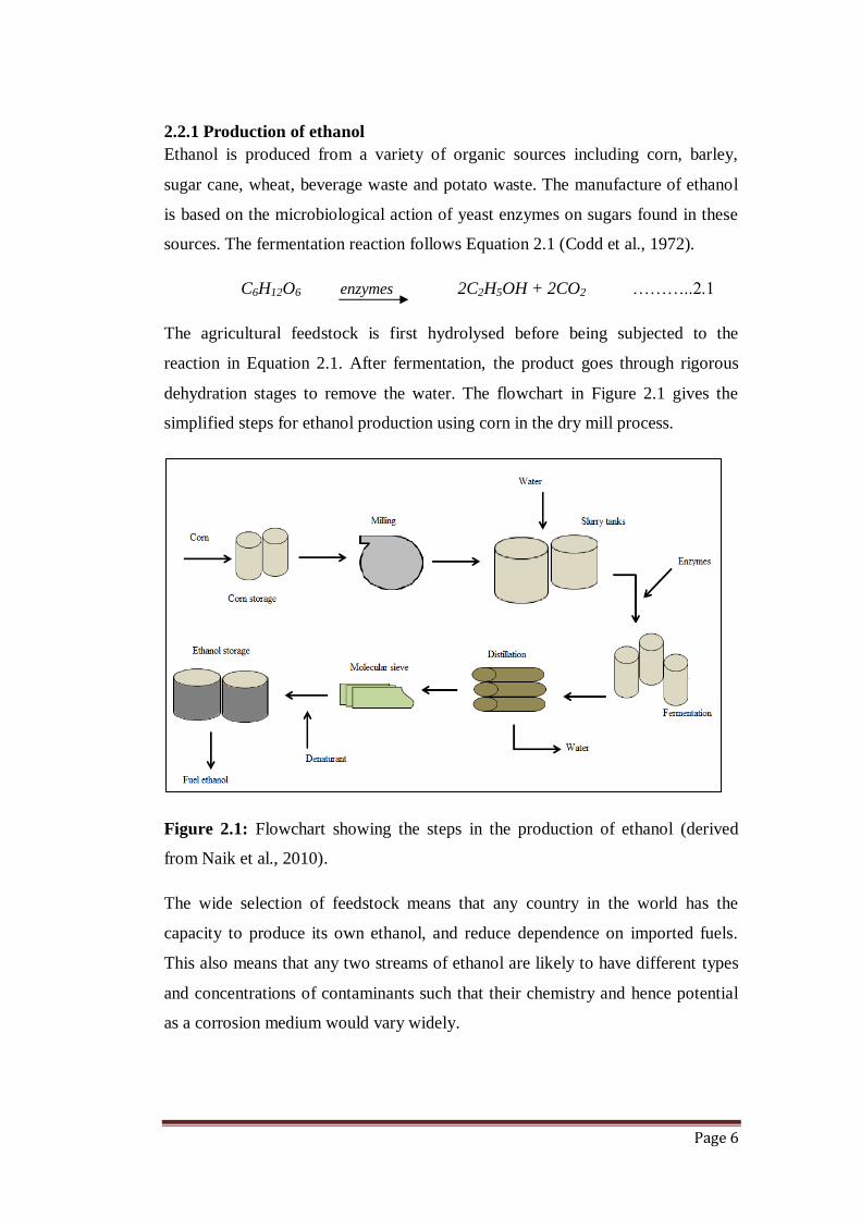
The agricultural feedstock is first hydrolysed before being subjected to the
reaction in Equation 2.1. After fermentation, the product goes through rigorous
dehydration stages to remove the water. The flowchart in Figure 2.1 gives the
simplified steps for ethanol production using corn in the dry mill process.
Figure 2.1: Flowchart showing the steps in the production of ethanol (derived
from Naik et al., 2010).
The wide selection of feedstock means that any country in the world has the
capacity to produce its own ethanol, and reduce dependence on imported fuels.
This also means that any two streams of ethanol are likely to have different types
and concentrations of contaminants such that their chemistry and hence potential
as a corrosion medium would vary widely.
Page 7
2.2.2 Chemical properties of ethanol
All alcohols, like water, are amphoteric. In the presence of water, alcohol will
either be reversibly protonated or will dissociate slightly as given in Equations
2.2 and 2.3 (McMurry, 2007).
...............…..…. 2.2
.......................... 2.3
where R is the alkyl group on ethanol. From these equations, it can be
inferred that ethanol is a protic medium and just like water, is capable of
sustaining electron transfer and ionization of hydrogen atoms (Kane et al., 2004).
This thus implies that ethanol can support corrosion processes. The effects of
water and oxygen on the chemical properties of ethanol are summarised below.
i. Ethanol and water
Ethanol is completely miscible in water since both solvents are polar in nature.
The two liquids form an azeotropic mixture at 96% ethanol. During manufacture,
ethanol and water are separated by azeotropic distillation techniques, namely
molecular sieving as mentioned in Figure 2.1. Despite this, ethanol rarely has zero
water. Ethanol is extremely hygroscopic in nature (Sridhar, 2006) and will absorb
huge quantities of water when exposed to humid conditions.
The presence of water in ethanol has the effect of increasing the dielectric
constant of ethanol (Faraji et al., 2009). Materials with a high dielectric constant
break down easier when subjected to an electric field than those with a low
dielectric constant. The consequence of this break down is an increased ability for
the material to facilitate the flow of charge through it, and thus conduct electricity.
Since increasing water content gives a corresponding increase in electrical
conductivity, it means that increasing water increases the risk of corrosion in
ethanol solutions.
The pKa of water is 15.74 while that of ethanol is 16 (McMurry, 2007). This
implies that water is a stronger acid than ethanol. Its presence in ethanol should
therefore increase the acidity of the solution.
Page 8
ii. Ethanol and oxygen
In fuels, the main benefit of ethanol is its ability to increase oxygen content and
thus ensure complete combustion. Ethanol has a very high solubility for oxygen.
At about 20⁰C, oxygen solubility in ethanol is 44 cm³/L compared to 6.4 cm³/L
for distilled water at the same temperature (Reseder, 1980). Considering this
difference, it should be expected that an increase in water content would markedly
reduce oxygen solubility in ethanol.
Taking the solubility of oxygen to be a direct reflection of oxygen concentration
in the solution, it follows therefore that the diffusion rates of oxygen in ethanol-
water mixtures will be lower than in anhydrous ethanol. This inference can be
supported by Fick’s law of diffusion described in Equation 2.4 where D is the
diffusion coefficient, dC is change in concentration and dx is the distance from
electrode surface.
.............................2.4
According to this equation, if the concentration of a species in the bulk solution is
high, then diffusion rates of that species will be high.
The oxidation of ethanol produces acetic acid as per Equation 2.5 (Tembe, 2010).
CH3CH2OH + O2 → CH3COOH + H2O ..………………2.5
Organic acids are weak acids and are generally regarded as non-corrosive. Yet,
they can hydrolyse well enough to act as true acids towards most metals
(Scribner, 2001). The pKa of acetic acid at 25⁰C is 4.75 and its pH is 2.4. The
oxidation of ethanol is thus associated with an increase in acidity and an increased
corrosion risk.
2.3 Corrosion reactions
The theory of corrosion states that corrosion proceeds by an electrochemical
reaction which can be divided into two or more oxidation and reduction reactions.
Page 9
A metal, M, corroding in neutral water would thus react as per Equations 2.6 and
2.7.
M → M+ + ē (oxidation/anodic) ……………….. 2.6
2H2O + 2ē → 2OH‾ (reduction/cathodic) ………..............2.7
When the metal, M, is not in equilibrium with its ions, for example when the
anodic reaction is much faster than the cathodic reaction, the electrode potential,
E, of M differs from its corrosion potential, Ecorr, by an amount known as the
overpotential or polarisation, η. This parameter is defined by Equations 2.8 and
2.9 (Roberge, 2008).
……………….. 2.8
………………… 2.9
In Equation 2.9, ηA is the activation polarization, ηC is the concentration
polarization and iR is the ohmic drop brought about by the electrical resistivity of
the environment. In practice, one of the three potentials in the equation
predominates (Codd et al., 1970; Simbi, 2006). This has led to the classification of
three types of corrosion reactions.
i. Charge transfer controlled
A charge (or electron) transfer controlled reaction is characterised by a large
activation potential, ηA. The activation potential of a corrosion reaction is a
measure of how hard the anodic and the cathodic reactions must be driven to
achieve the corrosion current and is strongly dependent on the composition of the
solution.
Anions of low molar polarisation, when absorbed onto metal surfaces, have a poor
tendency to promote electron exchange reactions and hence reduce the rate of
electron transfer (Clubley, 1988; Simbi, 2006). Such anions substantially increase
the activation potential and slow down corrosion processes. Inhibitors are
examples of species that cause charge transfer controlled reactions.
Page 10
Both water and ethanol have permanent dipoles arising from the asymmetric
bonds between the oxygen and the hydrogen atoms. However, water molecules
have a higher molar polarisation by virtue of their size. This implies that the
presence of water in ethanol would improve the alcohol’s tendency to promote
electron transfer processes and increase corrosion rates.
ii. Diffusion-controlled
During a corrosion process, there exists a deviation of the concentration of the
corroding species on the electrode surface from that in the bulk solution. This
variation is described by Fick’s law (Equation 2.4) and is characterised by the
concentration polarization, ηC. A corrosion reaction whereby the slowest step
involves a diffusion process is termed diffusion-controlled
(Roseblim et al., 1968). The rate of such a reaction is increased by agitating the
environment, increasing temperature and the concentration of the diffusing
species.
Diffusion-controlled reactions are characterised by a limiting current density
which is defined as the highest current density possible for a given electrode
reaction due to the limitations imposed by the diffusion velocity of the reacting
particles (Lapedes, 1978; Simbi, 2006). Corrosion processes of iron in water are
controlled by the diffusion rate of oxygen to the corroding surface (Fontana, 1986;
Revie, 2011) and the corrosion rate is usually determined by the limiting current
density for the cathodic reduction of oxygen.
The corrosion processes in ethanol-water solutions are likely to be diffusion
controlled given the low diffusion rates discussed in Section 2.2.2.
i. Mixed control
In mixed control processes, the rate of charge transfer is such that the
concentration of one of the species decreases significantly at the interface
(Pletcher, 1991) and differs greatly from its concentration in the bulk. This will
give rise to a concentration gradient: the driving force for diffusion. As such, the
Page 11
corrosion process is controlled by both the rate of charge transfer at the electrode
and the diffusion of species to the electrode surface.
2.4 Stress corrosion cracking
2.4.1 Definition of SCC
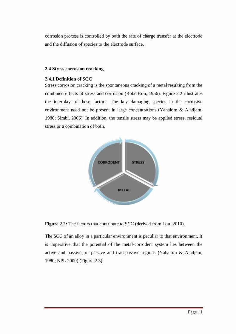
Stress corrosion cracking is the spontaneous cracking of a metal resulting from the
combined effects of stress and corrosion (Robertson, 1956). Figure 2.2 illustrates
the interplay of these factors. The key damaging species in the corrosive
environment need not be present in large concentrations (Yahalom & Aladjem,
1980; Simbi, 2006). In addition, the tensile stress may be applied stress, residual
stress or a combination of both.
Figure 2.2: The factors that contribute to SCC (derived from Lou, 2010).
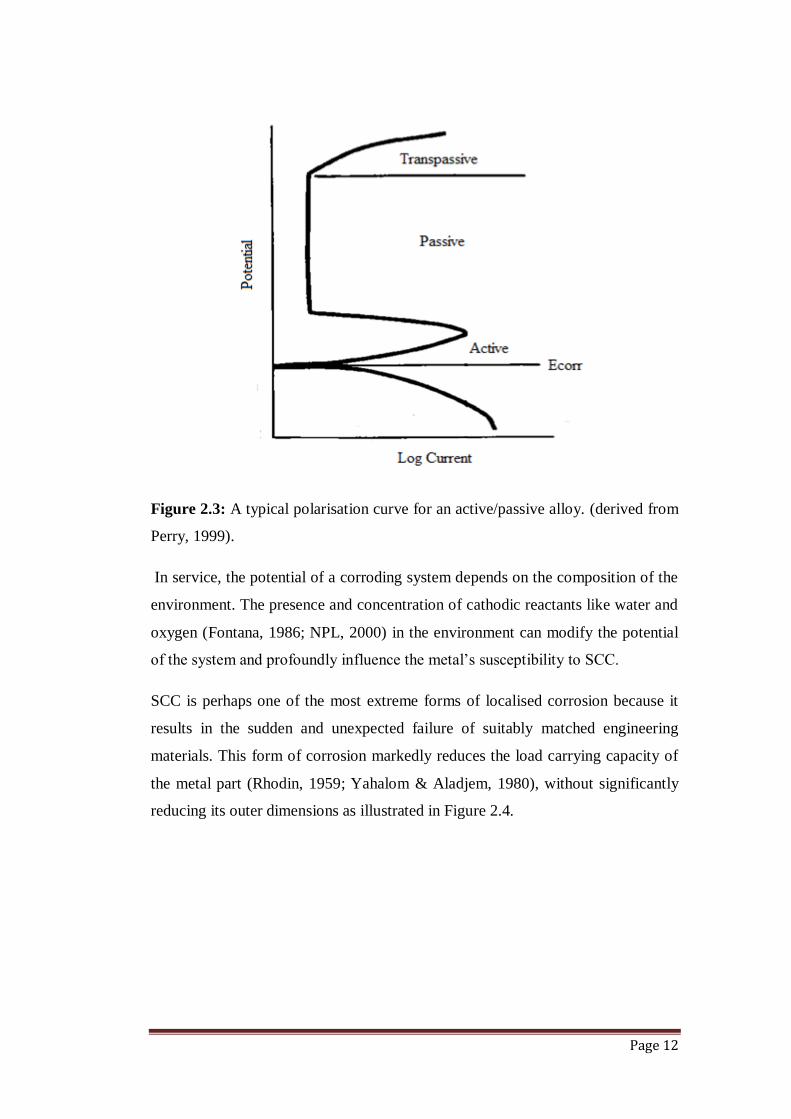
The SCC of an alloy in a particular environment is peculiar to that environment. It
is imperative that the potential of the metal-corrodent system lies between the
active and passive, or passive and transpassive regions (Yahalom & Aladjem,
1980; NPL 2000) (Figure 2.3).
Page 12
Figure 2.3: A typical polarisation curve for an active/passive alloy. (derived from
Perry, 1999).
In service, the potential of a corroding system depends on the composition of the
environment. The presence and concentration of cathodic reactants like water and
oxygen (Fontana, 1986; NPL, 2000) in the environment can modify the potential
of the system and profoundly influence the metal’s susceptibility to SCC.
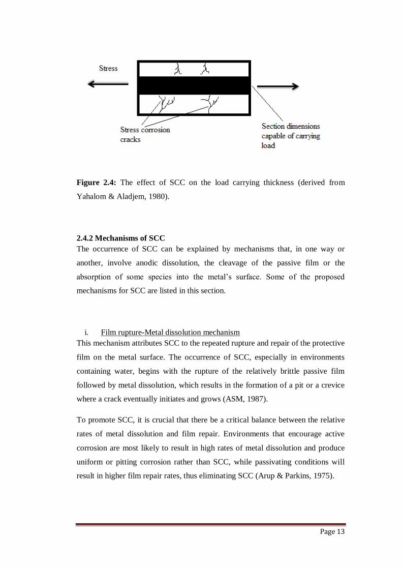
SCC is perhaps one of the most extreme forms of localised corrosion because it
results in the sudden and unexpected failure of suitably matched engineering
materials. This form of corrosion markedly reduces the load carrying capacity of
the metal part (Rhodin, 1959; Yahalom & Aladjem, 1980), without significantly
reducing its outer dimensions as illustrated in Figure 2.4.
Page 13
Figure 2.4: The effect of SCC on the load carrying thickness (derived from
Yahalom & Aladjem, 1980).
2.4.2 Mechanisms of SCC
The occurrence of SCC can be explained by mechanisms that, in one way or
another, involve anodic dissolution, the cleavage of the passive film or the
absorption of some species into the metal’s surface. Some of the proposed
mechanisms for SCC are listed in this section.
i. Film rupture-Metal dissolution mechanism
This mechanism attributes SCC to the repeated rupture and repair of the protective
film on the metal surface. The occurrence of SCC, especially in environments
containing water, begins with the rupture of the relatively brittle passive film
followed by metal dissolution, which results in the formation of a pit or a crevice
where a crack eventually initiates and grows (ASM, 1987).
To promote SCC, it is crucial that there be a critical balance between the relative
rates of metal dissolution and film repair. Environments that encourage active
corrosion are most likely to result in high rates of metal dissolution and produce
uniform or pitting corrosion rather than SCC, while passivating conditions will
result in higher film repair rates, thus eliminating SCC (Arup & Parkins, 1975).
Page 14
According to the film rupture-metal dissolution mechanism, it is necessary for the
metal to passivate in the given environment. Passivity is not an inherent metal
property (Uhlig, 1948), but depends entirely on the environment to which it is
exposed. Many substances are capable of producing some degree of passivity,
oxygen being the most common. However, for some metals like aluminium and
titanium (Brown, 1977) water has been observed to perform this function just as
well.
ii. Stress-sorption mechanism
In this mechanism, fractures result from the production of a brittle region at the
crack tip because of the absorption of specific species into the metal (Yahalom &
Aladjem, 1980). An example is hydrogen embrittlement. In acidic media,
hydrogen production may result from the cathodic reaction as shown in Equation
2.8.
2H+ + 2ē → H2 ………………………. 2.8
In neutral media, hydrogen ions may be produced by a chemical reaction between
the exposed metal and water within confined volumes such as crack tips and
crevices (Equation 2.9). The ions thus produced are subsequently reduced as per
Equation 2.8 to give hydrogen gas.
Fe2+
2H2O → Fe(OH)2 + 2H+ ………………………. 2.9
Hydrogen atoms, because of their small size, have a high diffusivity in the metal
lattice. The absorbed hydrogen atoms interact with strain bands in the crack tip
and reduce the surface energy, γ, in this region. This compromises the mechanical
properties of the metal by lowering the stress required to produce a brittle fracture.
iii. Electrochemical mechanism
The electrochemical theory of SCC proposes that in the alloy, there must exist the
susceptibility to selective corrosion along a more or less continuous path
(Uhlig, 1948). Microstructural differences give rise to electrochemically distinct
Page 15
regions (Arup & Parkins, 1975), especially where there is the segregation of one
species to the grain boundaries. Grain boundaries are usually anodic to the
material within the grains (ASM, 1987) and will therefore be preferentially
dissolved when exposed to the corrosive medium. This results in intergranular
corrosion and the extent of grain boundary penetration plays a significant role in
SCC susceptibility in the given media. The crack path coincides with the
corrosion path.
In low carbon steels, carbon tends to segregate to the ferrite grain boundaries as
carbon or carbide precipitates (Arup & Parkins, 1975). The carbon enriched
boundaries then become anodic to the adjacent grains, and the small anode to
cathode ratio that results becomes the driving force for intergranular corrosion.
Under the simultaneous influence of stress, the steel would fail by intergranular
SCC (IG-SCC).
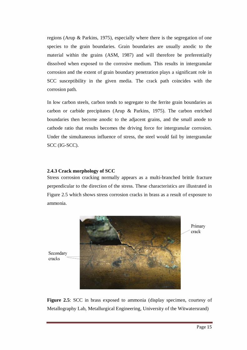
2.4.3 Crack morphology of SCC
Stress corrosion cracking normally appears as a multi-branched brittle fracture
perpendicular to the direction of the stress. These characteristics are illustrated in
Figure 2.5 which shows stress corrosion cracks in brass as a result of exposure to
ammonia.
Figure 2.5: SCC in brass exposed to ammonia (display specimen, courtesy of
Metallography Lab, Metallurgical Engineering, University of the Witwatersrand)
Page 16
Figure 2.5 shows secondary cracks branching off from the larger primary crack.
The corrosion products accumulate along the cracks and outline the morphology
of the secondary cracks. Considering Figures 2.4 and 2.5, the final fracture would
then consist of two distinct zones: a zone formed by the propagation of corrosion
cracking, with traces of corrosion products, and a zone produced by the
mechanical failure of the metal.
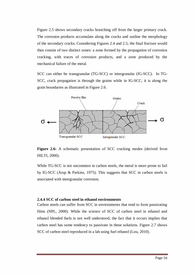
SCC can either be transgranular (TG-SCC) or intergranular (IG-SCC). In TG-
SCC, crack propagation is through the grains while in IG-SCC, it is along the
grain boundaries as illustrated in Figure 2.6.
Figure 2.6: A schematic presentation of SCC cracking modes (derived from
HILTI, 2000).
While TG-SCC is not uncommon in carbon steels, the metal is more prone to fail
by IG-SCC (Arup & Parkins, 1975). This suggests that SCC in carbon steels is
associated with intergranular corrosion.
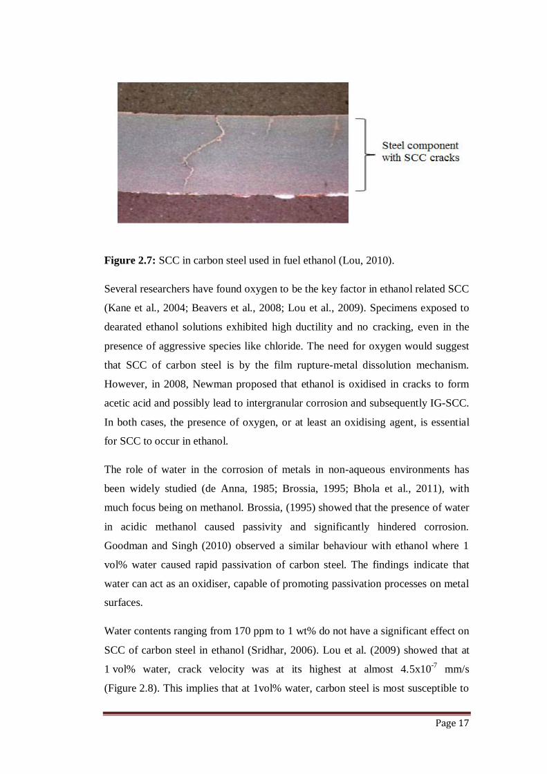
2.4.4 SCC of carbon steel in ethanol environments
Carbon steels can suffer from SCC in environments that tend to form passivating
films (NPL, 2000). While the science of SCC of carbon steel in ethanol and
ethanol blended fuels is not well understood, the fact that it occurs implies that
carbon steel has some tendency to passivate in these solutions. Figure 2.7 shows
SCC of carbon steel reproduced in a lab using fuel ethanol (Lou, 2010).
Page 17
Figure 2.7: SCC in carbon steel used in fuel ethanol (Lou, 2010).
Several researchers have found oxygen to be the key factor in ethanol related SCC
(Kane et al., 2004; Beavers et al., 2008; Lou et al., 2009). Specimens exposed to
dearated ethanol solutions exhibited high ductility and no cracking, even in the
presence of aggressive species like chloride. The need for oxygen would suggest
that SCC of carbon steel is by the film rupture-metal dissolution mechanism.
However, in 2008, Newman proposed that ethanol is oxidised in cracks to form
acetic acid and possibly lead to intergranular corrosion and subsequently IG-SCC.
In both cases, the presence of oxygen, or at least an oxidising agent, is essential
for SCC to occur in ethanol.
The role of water in the corrosion of metals in non-aqueous environments has
been widely studied (de Anna, 1985; Brossia, 1995; Bhola et al., 2011), with
much focus being on methanol. Brossia, (1995) showed that the presence of water
in acidic methanol caused passivity and significantly hindered corrosion.
Goodman and Singh (2010) observed a similar behaviour with ethanol where 1
vol% water caused rapid passivation of carbon steel. The findings indicate that
water can act as an oxidiser, capable of promoting passivation processes on metal
surfaces.
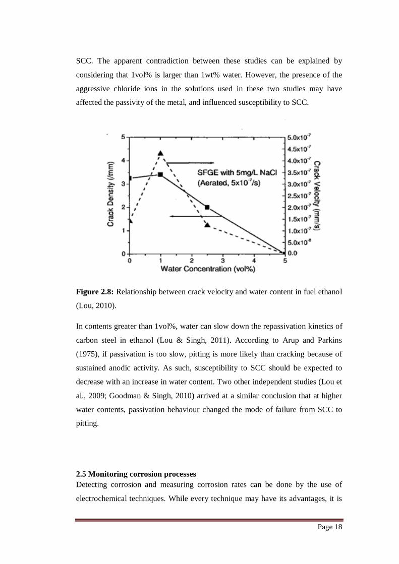
Water contents ranging from 170 ppm to 1 wt% do not have a significant effect on
SCC of carbon steel in ethanol (Sridhar, 2006). Lou et al. (2009) showed that at
1 vol% water, crack velocity was at its highest at almost 4.5x10⁻⁷
mm/s
(Figure 2.8). This implies that at 1vol% water, carbon steel is most susceptible to
Page 18
SCC. The apparent contradiction between these studies can be explained by
considering that 1vol% is larger than 1wt% water. However, the presence of the
aggressive chloride ions in the solutions used in these two studies may have
affected the passivity of the metal, and influenced susceptibility to SCC.
Figure 2.8: Relationship between crack velocity and water content in fuel ethanol
(Lou, 2010).
In contents greater than 1vol%, water can slow down the repassivation kinetics of
carbon steel in ethanol (Lou & Singh, 2011). According to Arup and Parkins
(1975), if passivation is too slow, pitting is more likely than cracking because of
sustained anodic activity. As such, susceptibility to SCC should be expected to
decrease with an increase in water content. Two other independent studies (Lou et
al., 2009; Goodman & Singh, 2010) arrived at a similar conclusion that at higher
water contents, passivation behaviour changed the mode of failure from SCC to
pitting.
2.5 Monitoring corrosion processes
Detecting corrosion and measuring corrosion rates can be done by the use of
electrochemical techniques. While every technique may have its advantages, it is
Page 19
essential to complement it with other measuring techniques. By so doing, a more
accurate picture of the electrode processes may be obtained.
2.5.1 Linear polarisation resistance
Linear polarisation resistance (LPR) measuring techniques involve an iR drop
through the electrolyte surrounding the electrode and/or through a surface film. It
is a useful method for determining instantaneous corrosion rates and is both rapid
and non-intrusive (Song & Saraswathy, 2000). In addition, LPR can give the
corrosion potential of a metal in contact with an electrolyte which is in fact, an
indication of the tendency of a metal to corrode in that environment.
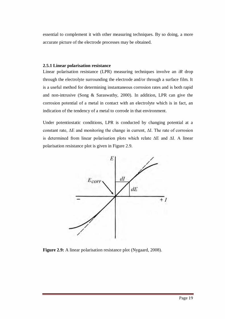
Under potentiostatic conditions, LPR is conducted by changing potential at a
constant rate, ΔE and monitoring the change in current, ΔI. The rate of corrosion
is determined from linear polarisation plots which relate ΔE and ΔI. A linear
polarisation resistance plot is given in Figure 2.9.
Figure 2.9: A linear polarisation resistance plot (Nygaard, 2008).
Page 20
The corrosion rate is expressed by the Stern-Geary equation
[
( )] (
) ..……………………. 2.10
In Equation 2.10, icorr is the corrosion current density, Rp is the polarisation
resistance and βa and βc are the anodic and cathodic Tafel constants respectively.
The value of Rp is the gradient of the linear polarisation plot (Figure 2.9) within
10-30 mV more noble or more active than Ecorr, the free corrosion potential.
The main limit of LPR is that it is often erroneous when used in environments in
which the electrolyte has significantly high resistivity. In such cases it should be
complimented by other electrochemical techniques such as EIS.
2.5.2 Electrochemical impedance spectroscopy
Electrochemical Impedance Spectroscopy (EIS), also referred to as AC impedance
analysis, is a technique used to investigate the corrosion behaviour of metals in
low conductivity solutions. It is a non-destructive technique in which a small
sinusoidal voltage is superiposed on an applied potential at predetermined discrete
frequencies. The current responses to these perturbations are used to determine
impedance (resistance), Z, as defined by Equation 2.11 (Pletcher, 1991).
E = IZ …………………….2.11
E is the applied voltage and I is the current. The analysis of EIS data involves the
use of passive elements like resistors, capacitors and inductors and these elements
represent some physical component of the corroding system. Listed below are
some of the common passive elements and their interpretation.
i. RΩ: Referred to as the ohmic resistance, RΩ is the resistance between the
working electrode and the reference electrode. It is used to characterise the
resistance of the solution and its value is determined at the high frequency
end of the impedance spectrum.
ii. Rct: Rct is the charge transfer resistance which characterises the electron
transfer process in corrosion.
Page 21
iii. Rp: Rp is the polarisation resistance that arises from the polarisation of the
working electrode. Polarisation resistance is related to the corrosion rate
by the Stern-Geary relationship given in Equation 2.10.
iv. Cdl: This refers to the double layer capacitance and is related to the double
layer formed as the ions in the solution approach the electrode surface
(Metrohm, 2011). The double layer capacitance is closely related to the
thickness, d, of the film formed on the surface by Equation 2.12 (Ebrahim
et al., 2012).
.............................................2.12
In this equation, εo and ε are the permittivity of air and the local dielectric
respectively and S is the surface area of the electrode.
v. W: Known as the Warburg impedance or the diffusion impedance, this
quantity models the diffusion of ionic species at the interface (Metrohm,
2011) and can be used to qualify diffusion controlled corrosion processes.
Experimental data from EIS is presented in a wide range of plots, but only two
will be discussed here.
i. The Nyquist plot
This is a plot of the imaginary component of impedance, Z″ against the real part
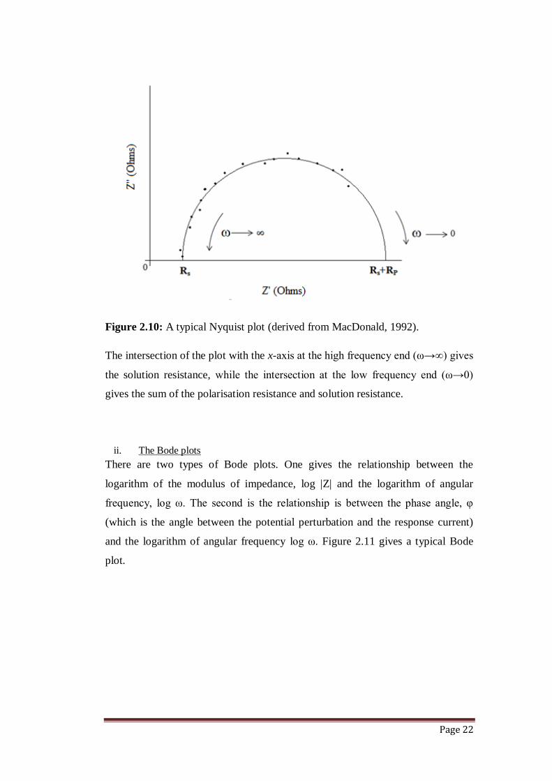
of impedance, Z′. A typical Nyquist plot is shown in Figure 2.10.
Page 22
Figure 2.10: A typical Nyquist plot (derived from MacDonald, 1992).
The intersection of the plot with the x-axis at the high frequency end (ω→∞) gives
the solution resistance, while the intersection at the low frequency end (ω→0)
gives the sum of the polarisation resistance and solution resistance.
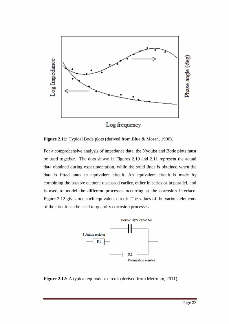
ii. The Bode plots
There are two types of Bode plots. One gives the relationship between the
logarithm of the modulus of impedance, log |Z| and the logarithm of angular
frequency, log ω. The second is the relationship is between the phase angle, φ
(which is the angle between the potential perturbation and the response current)
and the logarithm of angular frequency log ω. Figure 2.11 gives a typical Bode
plot.
Page 23
Figure 2.11: Typical Bode plots (derived from Blue & Moran, 1990).
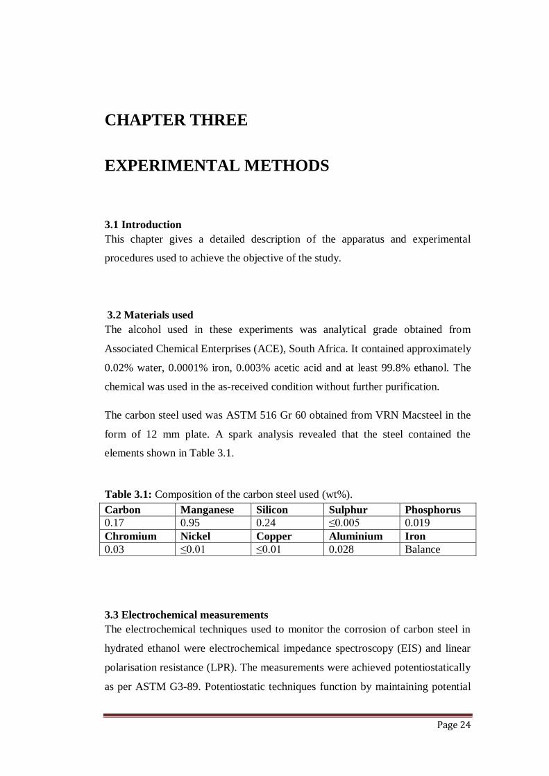
For a comprehensive analysis of impedance data, the Nyquist and Bode plots must
be used together. The dots shown in Figures 2.10 and 2.11 represent the actual
data obtained during experimentation, while the solid lines is obtained when the
data is fitted onto an equivalent circuit. An equivalent circuit is made by
combining the passive element discussed earlier, either in series or in parallel, and
is used to model the different processes occurring at the corrosion interface.
Figure 2.12 gives one such equivalent circuit. The values of the various elements
of the circuit can be used to quantify corrosion processes.
Figure 2.12: A typical equivalent circuit (derived from Metrohm, 2011).
Page 24
CHAPTER THREE
EXPERIMENTAL METHODS
3.1 Introduction
This chapter gives a detailed description of the apparatus and experimental
procedures used to achieve the objective of the study.
3.2 Materials used
The alcohol used in these experiments was analytical grade obtained from
Associated Chemical Enterprises (ACE), South Africa. It contained approximately
0.02% water, 0.0001% iron, 0.003% acetic acid and at least 99.8% ethanol. The
chemical was used in the as-received condition without further purification.
The carbon steel used was ASTM 516 Gr 60 obtained from VRN Macsteel in the
form of 12 mm plate. A spark analysis revealed that the steel contained the
elements shown in Table 3.1.
Table 3.1: Composition of the carbon steel used (wt%).
Carbon Manganese Silicon Sulphur Phosphorus
0.17 0.95 0.24 ≤0.005 0.019
Chromium Nickel Copper Aluminium Iron
0.03 ≤0.01 ≤0.01 0.028 Balance
3.3 Electrochemical measurements
The electrochemical techniques used to monitor the corrosion of carbon steel in
hydrated ethanol were electrochemical impedance spectroscopy (EIS) and linear
polarisation resistance (LPR). The measurements were achieved potentiostatically
as per ASTM G3-89. Potentiostatic techniques function by maintaining potential
Page 25
constant and measuring the current response. These methods were preferred to
galvanostatic techniques because the resulting data are easier to interpret and are
particularly useful when determining the effect of environmental changes on
reaction rates (Greene, 1965).
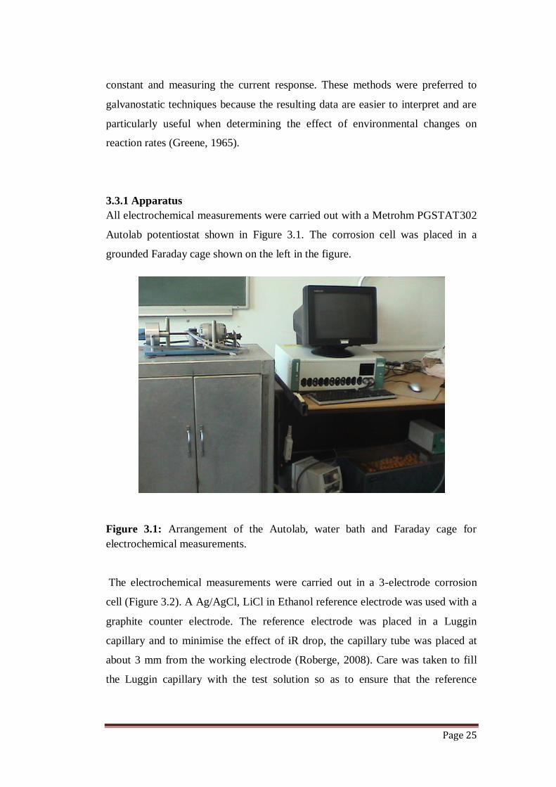
3.3.1 Apparatus
All electrochemical measurements were carried out with a Metrohm PGSTAT302
Autolab potentiostat shown in Figure 3.1. The corrosion cell was placed in a
grounded Faraday cage shown on the left in the figure.
Figure 3.1: Arrangement of the Autolab, water bath and Faraday cage for
electrochemical measurements.
The electrochemical measurements were carried out in a 3-electrode corrosion
cell (Figure 3.2). A Ag/AgCl, LiCl in Ethanol reference electrode was used with a
graphite counter electrode. The reference electrode was placed in a Luggin
capillary and to minimise the effect of iR drop, the capillary tube was placed at
about 3 mm from the working electrode (Roberge, 2008). Care was taken to fill
the Luggin capillary with the test solution so as to ensure that the reference
Page 26
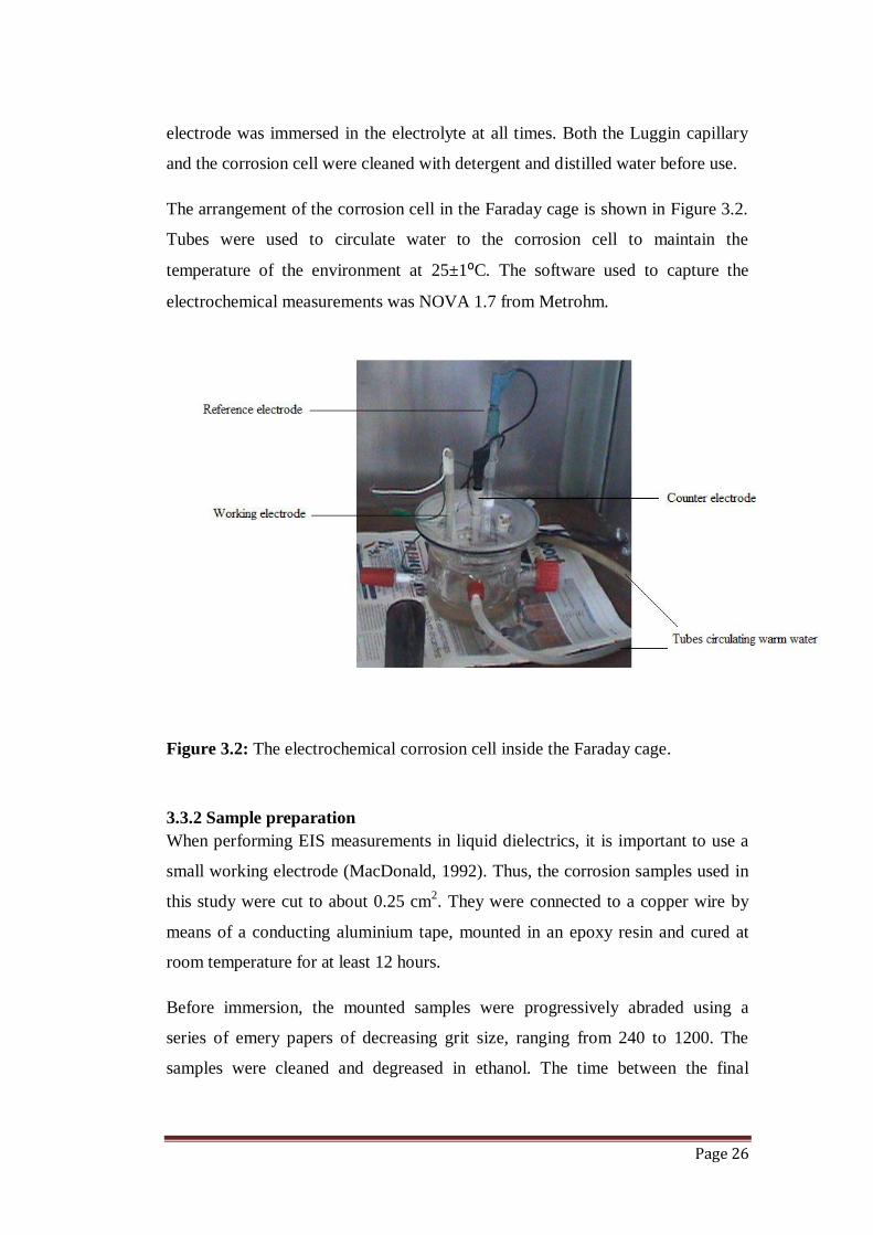
electrode was immersed in the electrolyte at all times. Both the Luggin capillary
and the corrosion cell were cleaned with detergent and distilled water before use.
The arrangement of the corrosion cell in the Faraday cage is shown in Figure 3.2.
Tubes were used to circulate water to the corrosion cell to maintain the
temperature of the environment at 25±1⁰C. The software used to capture the
electrochemical measurements was NOVA 1.7 from Metrohm.
Figure 3.2: The electrochemical corrosion cell inside the Faraday cage.
3.3.2 Sample preparation
When performing EIS measurements in liquid dielectrics, it is important to use a
small working electrode (MacDonald, 1992). Thus, the corrosion samples used in
this study were cut to about 0.25 cm2. They were connected to a copper wire by
means of a conducting aluminium tape, mounted in an epoxy resin and cured at
room temperature for at least 12 hours.
Before immersion, the mounted samples were progressively abraded using a
series of emery papers of decreasing grit size, ranging from 240 to 1200. The
samples were cleaned and degreased in ethanol. The time between the final
Page 27
surface preparation and the start of the experiment was kept to no more than 2
hours. This was done so as to improve repeatability.
3.3.3 Procedures
i. Linear polarisation resistance
The test environments were made by placing known volumes of water into a
500 ml beaker and filling up with ethanol to the 500 ml mark. No supporting
electrolytes or salts were added to the solution. The linear polarisation
measurements were carried out at a scan rate of 0.5 mV/s. Open circuit potential
(OCP) values were recorded at a 12 hour interval over a period of 72 hours.
ii. Electrochemical impedance
The solutions used were prepared as in the procedure for linear polarisation
resistance. Measurements were done at frequencies ranging from 80 Hz to
0.01 Hz at amplitudes of 10 mV. The low frequency limits were chosen to ensure
minimal changes in the system, and therefore guarantee linearity conditions. A
frequency response analyser, FRA, was used in conjunction with NOVA 1.7 to
collect impedance data.
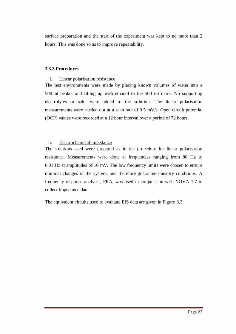
The equivalent circuits used to evaluate EIS data are given in Figure 3.3.
Page 28
Figure 3.3: Equivalent circuits used to evaluate EIS data
Circuits (a) and (b) were used to analyse the data obtained from experimentation
in ethanol solutions containing no water and with 1 vol% water. These circuits are
non-distinguishable (Bio-Logic, 2011) and are therefore interchangeable. In
circuit (b), R1 is equivalent to RΩ, the solution resistance while R2 is equal to the
polarisation resistance, Rp. In circuit (a), R1 is equivalent to Rp while the solution
resistance is expressed by Equation 3.1 (Bio-Logic, 2011)
……………………………… 3.1
For the analysis of carbon steel specimens in ethanol with 2.5 and 5 vol% water,
Circuit (c) was used. The choice of the circuits was based on the shapes of the
Nyquist curves obtained in the preliminary stages of the study. The curves for the
specimens in the solutions with 2.5 and 5 vol% water were characterised by a
Warburg slope thus necessitating the integration of the Warburg impedance into
Circuit (c).
Page 29
The double layer capacitance was calculated using Equation 3.2.
…………………………………….3.2
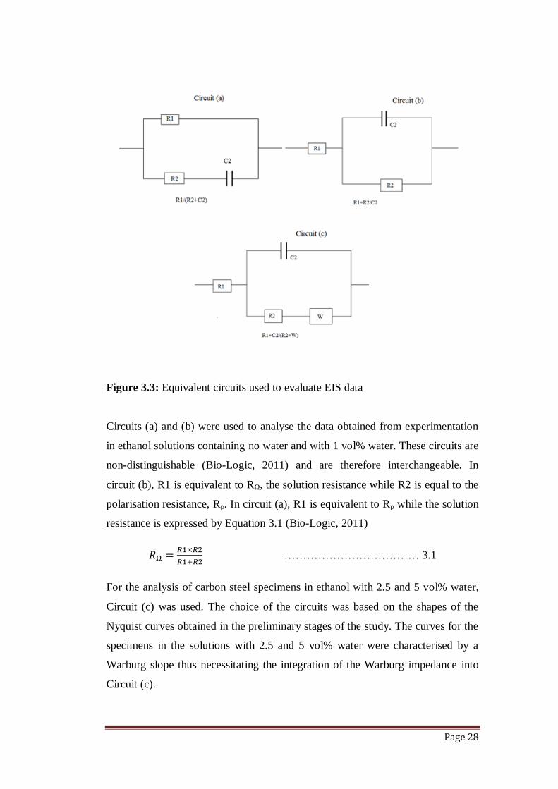
3.3.4 Repeatability of the potentiostat
The precision of a measuring technique lies in its ability to reproduce its own
results (Shoukri, 2004). The repeatability of the potentiostatic measuring method
was determined by carrying out two OCP tests in anhydrous ethanol. Presented in
Table 3.2 are the results of the statistical analysis of the obtained results.
Table 3.2: Statistical analysis of repeatability test results
Time
(h)
First test
(mV)
Second test
(mV) Average OCP (mV) Difference
0 217 201 209.0 -16
12 281 282 281.5 1
24 282 293 287.5 11
36 289 308 298.5 19
48 271 290 280.5 19
60 300 311 305.5 11
72 305 314 309.5 9
Mean Difference 7.7
Standard deviation
of difference 12.1
The standard deviation of the differences is 12.1 and the coefficient of
repeatability, r, is twice this value (24.2mV).
Mean difference is the mean of the differences of the results of the two tests. In
this case, the mean is 7.7. Since the same method was used, under identical
conditions and by the same researcher, the mean difference should ideally be zero.
However, the mean difference in this analysis is not significantly further from
Page 30
zero. Given this, the repeatability and hence precision of the measuring technique
is fairly good.
3.4 Slow strain-rate test
The criterion given in the NACE standard TM0111-2011 was used to
characterise SCC susceptibility of carbon steel in various ethanol-water
solutions. The possibility that specimen failure under tensile loading may be as
a consequence of simple void coalescence and not SCC was considered, and
metallographic examination, by use of optical and scanning electron
microscopes (SEM), was done to confirm the occurrence of SCC.
3.4.1 Apparatus
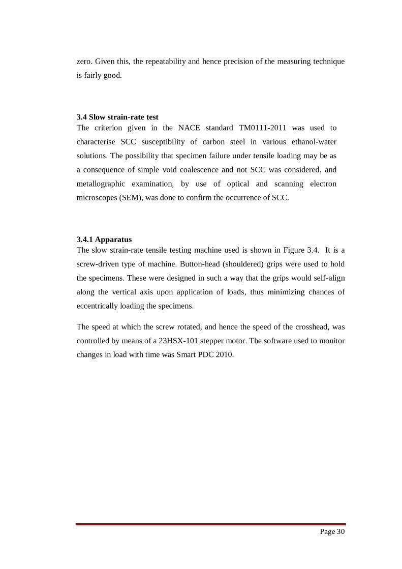
The slow strain-rate tensile testing machine used is shown in Figure 3.4. It is a
screw-driven type of machine. Button-head (shouldered) grips were used to hold
the specimens. These were designed in such a way that the grips would self-align
along the vertical axis upon application of loads, thus minimizing chances of
eccentrically loading the specimens.
The speed at which the screw rotated, and hence the speed of the crosshead, was
controlled by means of a 23HSX-101 stepper motor. The software used to monitor
changes in load with time was Smart PDC 2010.
Page 31
Figure 3.4: The tensile testing machine for SSRT without the corrosion cell.
A signal generator, together with a driving circuit consisting of a Gecko G230V
stepper drive, an 8A PSU board and a 32VAC transformer, was used to drive the
motor. The stepper motor-signal generator combination was calibrated to
determine the variation of strain-rate with the frequency of the generated pulse.
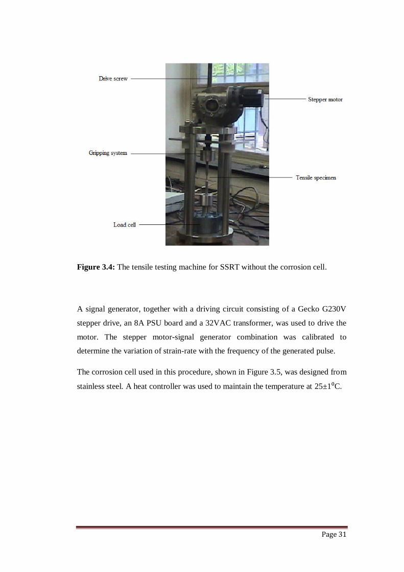
The corrosion cell used in this procedure, shown in Figure 3.5, was designed from
stainless steel. A heat controller was used to maintain the temperature at 25±1⁰C.
Page 32
Figure 3.5: SSRT corrosion cell used in the tensile test.
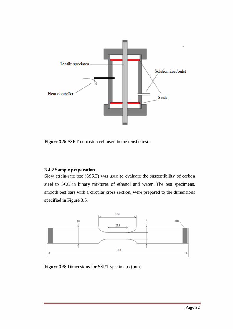
3.4.2 Sample preparation
Slow strain-rate test (SSRT) was used to evaluate the susceptibility of carbon
steel to SCC in binary mixtures of ethanol and water. The test specimens,
smooth test bars with a circular cross section, were prepared to the dimensions
specified in Figure 3.6.
Figure 3.6: Dimensions for SSRT specimens (mm).
Page 33
The sample shoulders were made quite long, 0.5 times longer than the corrosion
cell, to avoid galvanic corrosion between the specimen and the stainless steel
grips. The specimens were ground with emery paper of 1200 grit size and the
direction of grinding was parallel to the longitudinal axis of the tensile pieces.
This direction was maintained to avoid inducing circumferential dents and
stress raisers, thus ensuring that any surface cracks perpendicular to the stress
would be as a result of SCC. After grinding, the specimens were carefully
cleaned with ethanol and dried in a stream of compressed air.
3.4.3 Procedures
i. Calibration of the stepper motor
It is not stress per se, but the plastic strain that it produces (Shier et al., 1994)
that is responsible for SCC, and the propagation of cracks is dependent on the
rate of metal exposure by plastic strain. A slow strain-rate will allow adequate
repassivation of the crack tip (Jarvis, 1994) and suppress SCC. On the other
hand, a high strain-rate will result in a ductile fracture, as the rate of
electrochemical reactions will be too slow to enable repassivation and therefore
the propagation of SCC. In this study, strain-rates in order of 10μ/s were
chosen.
ii. SSRT
The test environment was made by placing known volumes of water in a
measuring cylinder and adding enough ethanol to make a 100 ml solution. The
corrosion cell was filled to about 90% volume, and the variation in the load
with time was recorded at 15 minute intervals. To avoid trapping water, the
corrosion cell was filled with ethanol and soaked for at least 8 hours before the
actual test. A baseline test was carried out in air, using a tensile specimen made
from ASTM 516. The results obtained in the tests in different ethanol solutions
were compared to the results the baseline test.
Page 34
3.5 Solution characterisation
The properties of the ethanol-water solutions were characterised in terms of
acidity, oxygen content and electrical conductivity. The solutions were prepared
from analytical grade ethanol and distilled water.
3.5.1 Apparatus
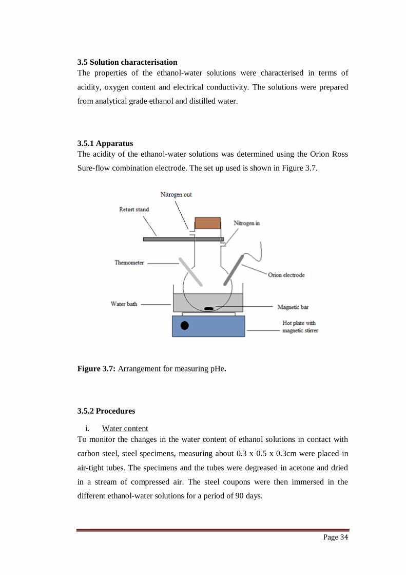
The acidity of the ethanol-water solutions was determined using the Orion Ross
Sure-flow combination electrode. The set up used is shown in Figure 3.7.
Figure 3.7: Arrangement for measuring pHe.
3.5.2 Procedures
i. Water content
To monitor the changes in the water content of ethanol solutions in contact with
carbon steel, steel specimens, measuring about 0.3 x 0.5 x 0.3cm were placed in
air-tight tubes. The specimens and the tubes were degreased in acetone and dried
in a stream of compressed air. The steel coupons were then immersed in the
different ethanol-water solutions for a period of 90 days.
Page 35
Sodium chloride is sparingly soluble in ethanol (at 0.52 g/L), but is highly soluble
in water (at 359 g/L). The difference in the solubility is what was used to estimate
the water content in solutions containing unknown compositions of ethanol and
water. A calibration curve relating solubility as a function of water content was
generated using known mixtures of ethanol and water. This curve was then used
to determine the composition of unknown mixtures of ethanol and water. The
exact procedure is outlined in Appendix A.
ii. Conductivity and dissolved oxygen
The conductivity and dissolved oxygen were measured using probe type meters.
In both cases, the readings were noted after 30 s of immersion.
iii. Acidity
The acidity of the ethanol mixtures was monitored by pHe as prescribed in the
ASTM D6423 standard. The parameter pHe is a measure of the acid strength of
alcohol fuels as defined by the said standard. For each solution sample, successive
repeats were taken and the four values whose difference did not exceed 0.29 were
averaged. The pHe values were taken before and after immersion.
3.6 Metallographic analysis
The occurrence of SCC was confirmed using a stereo microscope and a scanning
electron microscope (SEM).
3.6.1 Apparatus
A TOPCON SM-510 scanning electron microscope made by Oxford Instruments
was used. The microscope, with a tungsten filament, was continuously cooled
with liquid nitrogen and used a spot size of 10 mm2. Analysis was performed with
Oxford Link Isis and Link Tetra software operating on a HP work station.
Page 36
Visual inspection of the fractured and the corroded specimens was performed on a
stereo microscope equipped with a Nikon SMZ 745T camera. The camera was
operated by NIS Elements (Version 4) imaging software.
3.6.2 Procedures
The carbon steel specimens were stored in a desiccator immediately after slow
strain-rate testing. Before examination, the samples were cleaned in acetone in an
ultrasonic cleaner for 20 minutes.
3.7 Immersion test
An immersion test was carried out to compliment corrosion rates determined by
electrochemical methods. The immersion tests were performed under static
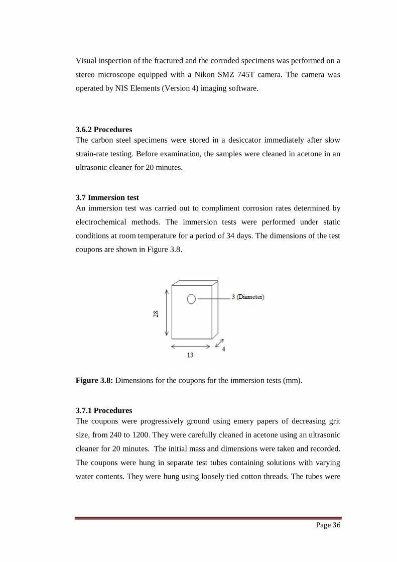
conditions at room temperature for a period of 34 days. The dimensions of the test
coupons are shown in Figure 3.8.
Figure 3.8: Dimensions for the coupons for the immersion tests (mm).
3.7.1 Procedures
The coupons were progressively ground using emery papers of decreasing grit
size, from 240 to 1200. They were carefully cleaned in acetone using an ultrasonic
cleaner for 20 minutes. The initial mass and dimensions were taken and recorded.
The coupons were hung in separate test tubes containing solutions with varying
water contents. They were hung using loosely tied cotton threads. The tubes were
Page 37
sealed to ensure that any oxygen in the solution was from the water. After the
immersion period, the specimens were cleaned and their masses recorded.
The corrosion rates were calculated as per Equation 3.3 (Obuka et al, 2012).
( )
………………………….. 3.3
K is a constant of unit conversion and its value was quoted as (Van
der Merwe, 2011). The parameters mb and ma are the mass of the coupon before
and after exposure respectively, while A is the exposed area, Δt, the exposure time
in hours and ρ is the density of the coupon.
Page 38
CHAPTER FOUR
RESULTS AND DISCUSSION:
CORROSION CHARACTERISATION
4.1 Introduction
This chapter presents and discusses the results obtained from the electrochemical
techniques used to evaluate the corrosion of carbon steel in the various solutions
of ethanol and water. The evolution of conductivity, dissolved oxygen and pHe of
the different test environments with time was also analysed in the bid to explain
the observed corrosion behaviour.
4.2 Solution characterisation
4.2.1 Conductivity
The conductivity of the ethanol-water solutions was measured as per the
procedure in Section 3.5.2 and the results are presented in Table 4.1 and Figure
4.1.
Page 39
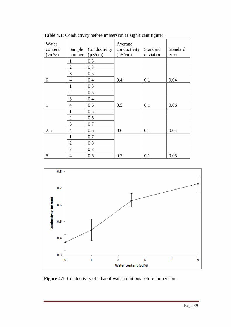
Table 4.1: Conductivity before immersion (1 significant figure).
Water
content
(vol%)
Sample
number
Conductivity
(µS/cm)
Average
conductivity
(µS/cm)
Standard
deviation
Standard
error
0
1 0.3
0.4 0.1 0.04
2 0.3
3 0.5
4 0.4
1
1 0.3
0.5 0.1 0.06
2 0.5
3 0.4
4 0.6
2.5
1 0.5
0.6 0.1 0.04
2 0.6
3 0.7
4 0.6
5
1 0.7
0.7 0.1 0.05
2 0.8
3 0.8
4 0.6
Figure 4.1: Conductivity of ethanol-water solutions before immersion.
Page 40
The increase in water content increased the conductivity of ethanol-water
mixtures from 0.4 µS/cm at 0 vol% water to 0.7 µS/cm at 5 vol% water. Electrical
conductivity in a solution occurs when there are ionisable species in the solution
capable of providing mobile ions. The observed conductivity trend could be
because of the autoprotolysis of water according to Equation 4.1.
2H2O ↔ H3O+ + OH‾ …………………….. 4.1
Ethanol is also a protic solvent capable of self-dissociation by Equation 4.2
(Metzge, 2012)
2C2H5OH ↔ C2H5OH2+ + C2H5O
‾ ……………………4.2
However, the ionic products formed by Equation 4.2 are much fewer as evidenced
by the low ion product constant (Ks) shown in Table 4.2.
Table 4.2: Ion product of water and ethanol.
Solvent Ion product (Ks)
C2H5OH 10‾19
H2O 10‾14
The increase in the concentration of ionic products produced by the autoprotolysis
of water leads to an increase in the dielectric constant of ethanol (Section 2.2.2)
and therefore electrical conductivity. The trend observed in Figure 4.1 is in
agreement with surveyed literature (ORNL, 2008; Spitze et al., 2009), and that of
the solution resistance as obtained by EIS (Table 4.3 and Figure 4.2).
Page 41
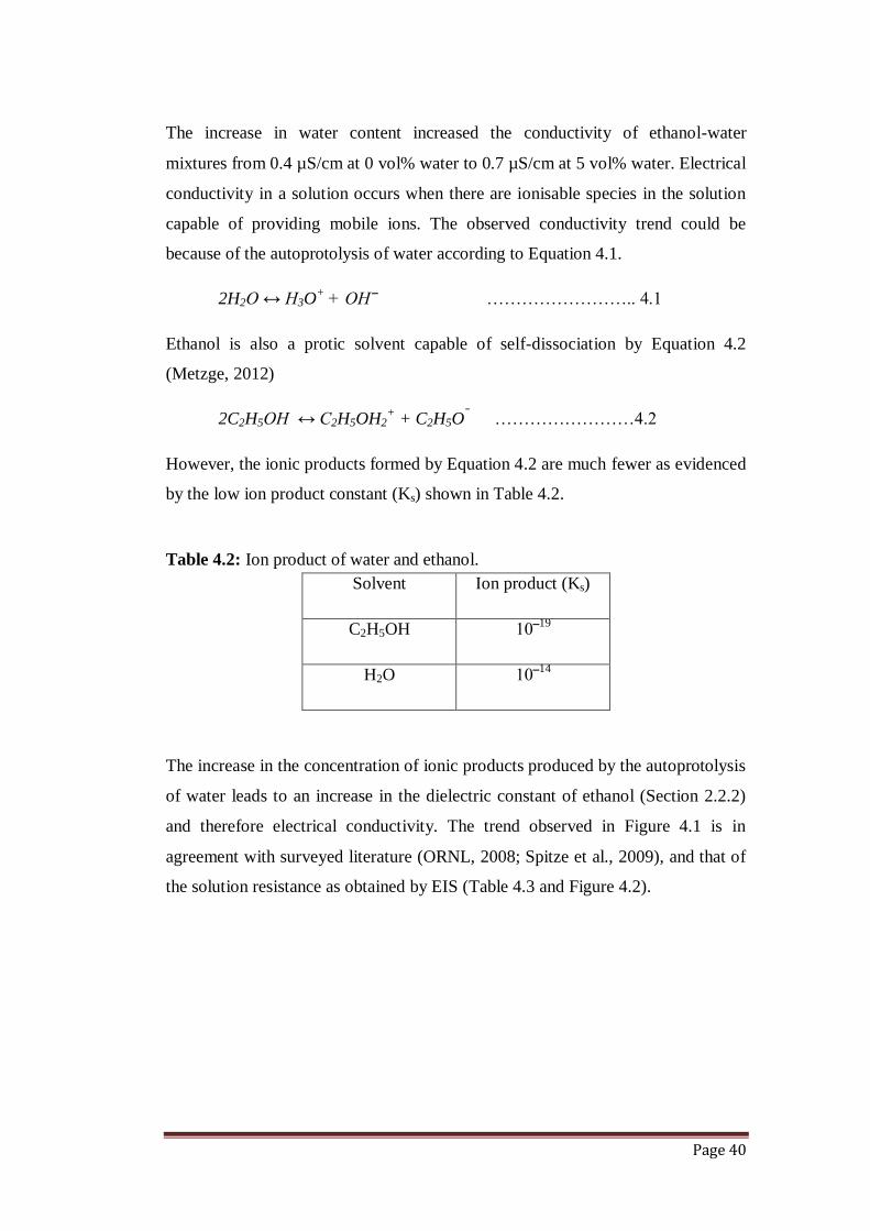
Table 4.3: Solution resistance as measured by EIS
Sample
number No water
1 vol%
water
2.5 vol%
water
5 vol%
water
1 1.53E+06 9.47E+05 3.60E+05 1.24E+05
2 1.44E+06 4.08E+05 3.17E+05 1.64E+05
3 3.76E+05 7.37E+05 3.27E+05 2.55E+05
4 6.75E+05 6.51E+05 3.16E+05 3.80E+05
5 1.21E+06 4.51E+04 3.15E+05 2.85E+05
6 6.08E+05 5.72E+05 3.35E+05 1.54E+05
Average 9.73E+05 5.60E+05 3.28E+05 2.27E+05
Standard
deviation 4.82E+05 3.09E+05 1.74E+04 9.74E+04
Standard
error 2.41E+05 1.55E+05 8.68E+03 4.87E+04
Figure 4.2: Solution resistance measured by EIS.
Solution resistance is inversely proportional to conductivity. As such, the trend in
Figure 4.2 shows an increased conductivity with increase in water content. The
electrical conductivity of the solutions was also measured at the end of the
immersion period. It was found to be significantly higher than the initial
conductivity values. Table 4.4 and Figure 4.3 show the results of the experiment.
0.0E+00
2.0E+05
4.0E+05
6.0E+05
8.0E+05
1.0E+06
1.2E+06
1.4E+06
0 1 2 3 4 5
Res
ista
nce
(Ω)
Water content (vol%)
Page 42
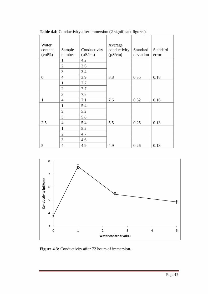
Table 4.4: Conductivity after immersion (2 significant figures).
Water
content
(vol%)
Sample
number
Conductivity
(µS/cm)
Average
conductivity
(µS/cm)
Standard
deviation
Standard
error
0
1 4.2
3.8 0.35 0.18
2 3.6
3 3.4
4 3.9
1
1 7.7
7.6 0.32 0.16
2 7.7
3 7.8
4 7.1
2.5
1 5.4
5.5 0.25 0.13
2 5.2
3 5.8
4 5.4
5
1 5.2
4.9 0.26 0.13
2 4.7
3 4.6
4 4.9
Figure 4.3: Conductivity after 72 hours of immersion.
3
4
5
6
7
8
0 1 2 3 4 5
Co
nd
uct
ivit
y (µ
S/cm
)
Water content (vol%)
Page 43
The observed values were too high to be explained by the autoprotolysis of water,
or the increase in the dielectric constant of ethanol with water percentage. As
such, the source of this high electrical conductivity was not the increasing water
content, but rather the presence of corrosion products. The major corrosion
product was likely to contain ferric ions, which have a high mobility and electrical
conductivity.
Besides being an indication of the risk of corrosion in a solution, electrical
conductivity can be a reflection of the concentration of the conducting ions in the
solution (Codd et al., 1970; Spitze et al., 2009). From Figure 4.3, the conductivity
of the solution with 1 vol% water had the highest conductivity of 7.6 µS/cm,
implying the highest concentration of ferric ions. The extent of corrosion in this
solution would be expected to be severe.
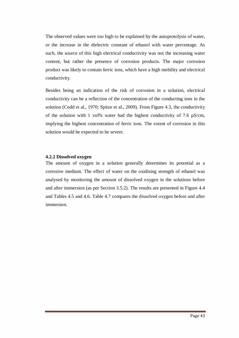
4.2.2 Dissolved oxygen
The amount of oxygen in a solution generally determines its potential as a
corrosive medium. The effect of water on the oxidising strength of ethanol was
analysed by monitoring the amount of dissolved oxygen in the solutions before
and after immersion (as per Section 3.5.2). The results are presented in Figure 4.4
and Tables 4.5 and 4.6. Table 4.7 compares the dissolved oxygen before and after
immersion.
Page 44
Table 4.5: Dissolved oxygen before immersion.
Water
content
(vol%)
Sample
number
Dissolved
oxygen
(mg/L)
Average
dissolved
oxygen
(mg/L)
Standard
deviation
Standard
error
0
1 5.85
6.00 0.15 0.08
2 6.17
3 6.09
4 5.90
1
1 6.12
6.09 0.28 0.14
2 6.46
3 5.81
4 5.95
2.5
1 6.20
6.11 0.15 0.08
2 6.16
3 5.88
4 6.18
5
1 6.00
6.45 0.52 0.26
2 6.82
3 6.98
4 6.00
Figure 4.4: Variation of dissolved oxygen (DO) with time and water content.
Page 45
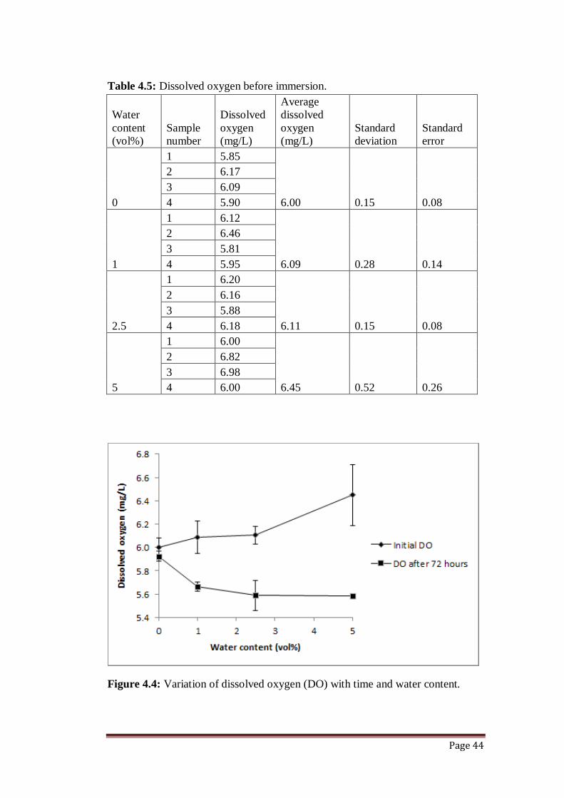
Table 4.6: Dissolved oxygen after 72 hours of immersion.
Water
content
(vol%)
Sample
number
Dissolved
oxygen
(mg/L)
Average
dissolved
oxygen
(mg/L)
Standard
deviation
Standard
error
0
1 6.03
5.93 0.09 0.04
2 5.90
3 5.82
4 5.95
1
1 5.76
5.66 0.08 0.04
2 5.59
3 5.69
4 5.61
2.5
1 5.58
5.59 0.03 0.01
2 5.60
3 5.62
4 5.56
5
1 5.55
5.58 0.04 0.02
2 5.63
3 5.54
4 5.61
Table 4.7: Comparison of dissolved oxygen before and after immersion.
Water content
(vol%)
Initial
dissolved
oxygen (mg/L)
Dissolved
oxygen after 72
hours (mg/L)
Percentage
difference (%)
0 6.00 5.93 1.17
1 6.09 5.66 7.06
2.5 6.11 5.59 8.51
5 6.45 5.58 13.49
Before immersion, there was an increase in the quantity of dissolved oxygen with
increase in water added. The trend observed was expected, since water contains
dissolved oxygen. As such, an increase in water will result in an increase in the
oxidising strength of ethanol-water mixtures. However, the content of dissolved
oxygen decreased with time, with the dissolved oxygen in ethanol containing
5 vol% water decreasing by as much as 13% after 72 hours of immersion.
Page 46
The concentration of oxygen in undiluted ethanol changed by only 0.078 mg/L
over the 72 hours of immersion. This slight change could be due to the fact that
anhydrous ethanol is hygroscopic, and the absorbed water ensures a constant
replenishment of dissolved oxygen. It is likely that the presence of water in
ethanol reduced its affinity for water vapour, and therefore its ability to replenish
any oxygen consumed by corrosion processes.
Perry (1999) showed that oxidising substances do not always accelerate corrosion
processes, but may retard them if the oxidising substance can form and preserve a
protective film on the material’s surface. The ability of the oxidising agent to
preserve a protective film depends primarily on the rate at which it is replenished
at the corrosion interface. A limited supply of the oxidising species can be
detrimental in so far as maintaining a passive state is concerned. Given this, the
poor replenishment of oxygen in ethanol-water mixtures with increased water
contents would mean reduced ability to repair any passive films broken down,
either by localised dissolution or by mechanical rupture.
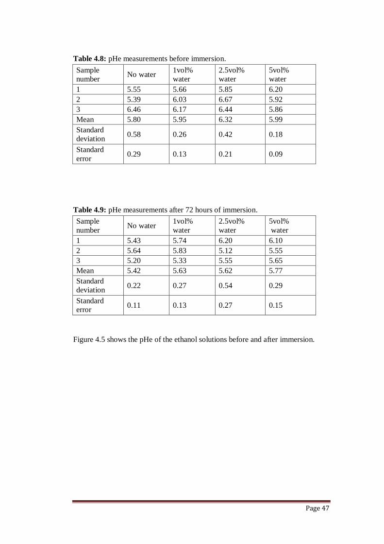
4.2.3 Acidity
The acidity of a solution can be used to qualify its potential as a corrosive
medium. In ethanol, this acidity is quantified by pHe which is, as is the case with
aqueous solutions, the negative logarithm of the activity of hydrogen ions in the
ethanol solution. On the pHe scale, 9.6 at 25⁰C is neutral, and a pHe of 6 is
considered highly acidic (Kane et al., 2004; Spitzer et al., 2009). Tables 4.8 and
4.9 present the results obtained in the experiment.
Page 47
Table 4.8: pHe measurements before immersion.
Sample
number No water
1vol%
water
2.5vol%
water
5vol%
water
1 5.55 5.66 5.85 6.20
2 5.39 6.03 6.67 5.92
3 6.46 6.17 6.44 5.86
Mean 5.80 5.95 6.32 5.99
Standard
deviation 0.58 0.26 0.42 0.18
Standard
error 0.29 0.13 0.21 0.09
Table 4.9: pHe measurements after 72 hours of immersion.
Sample
number No water
1vol%
water
2.5vol%
water
5vol%
water
1 5.43 5.74 6.20 6.10
2 5.64 5.83 5.12 5.55
3 5.20 5.33 5.55 5.65
Mean 5.42 5.63 5.62 5.77
Standard
deviation 0.22 0.27 0.54 0.29
Standard
error 0.11 0.13 0.27 0.15
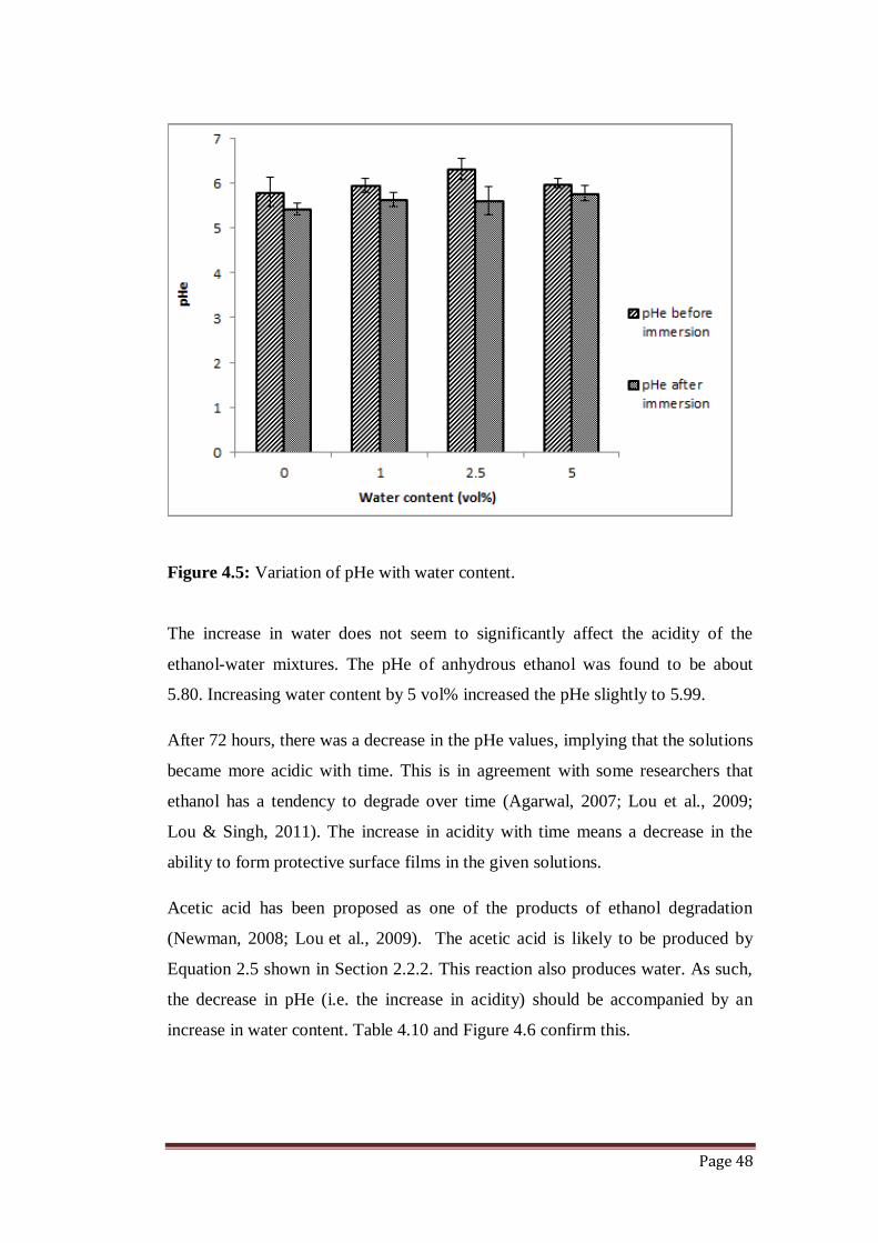
Figure 4.5 shows the pHe of the ethanol solutions before and after immersion.
Page 48
Figure 4.5: Variation of pHe with water content.
The increase in water does not seem to significantly affect the acidity of the
ethanol-water mixtures. The pHe of anhydrous ethanol was found to be about
5.80. Increasing water content by 5 vol% increased the pHe slightly to 5.99.
After 72 hours, there was a decrease in the pHe values, implying that the solutions
became more acidic with time. This is in agreement with some researchers that
ethanol has a tendency to degrade over time (Agarwal, 2007; Lou et al., 2009;
Lou & Singh, 2011). The increase in acidity with time means a decrease in the
ability to form protective surface films in the given solutions.
Acetic acid has been proposed as one of the products of ethanol degradation
(Newman, 2008; Lou et al., 2009). The acetic acid is likely to be produced by
Equation 2.5 shown in Section 2.2.2. This reaction also produces water. As such,
the decrease in pHe (i.e. the increase in acidity) should be accompanied by an
increase in water content. Table 4.10 and Figure 4.6 confirm this.
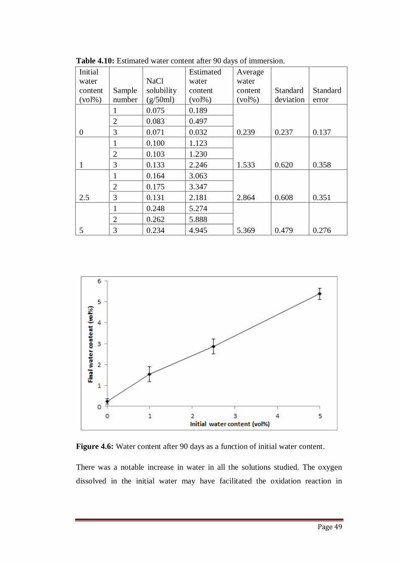
Page 49
Table 4.10: Estimated water content after 90 days of immersion.
Initial
water
content
(vol%)
Sample
number
NaCl
solubility
(g/50ml)
Estimated
water
content
(vol%)
Average
water
content
(vol%)
Standard
deviation
Standard
error
0
1 0.075 0.189
0.239 0.237 0.137
2 0.083 0.497
3 0.071 0.032
1
1 0.100 1.123
1.533 0.620 0.358
2 0.103 1.230
3 0.133 2.246
2.5
1 0.164 3.063
2.864 0.608 0.351
2 0.175 3.347
3 0.131 2.181
5
1 0.248 5.274
5.369 0.479 0.276
2 0.262 5.888
3 0.234 4.945
Figure 4.6: Water content after 90 days as a function of initial water content.
There was a notable increase in water in all the solutions studied. The oxygen
dissolved in the initial water may have facilitated the oxidation reaction in
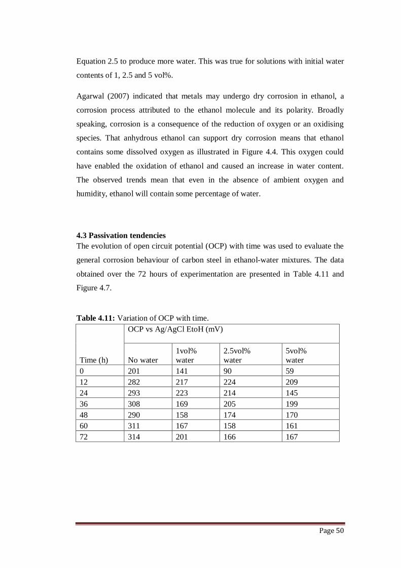
Page 50
Equation 2.5 to produce more water. This was true for solutions with initial water
contents of 1, 2.5 and 5 vol%.
Agarwal (2007) indicated that metals may undergo dry corrosion in ethanol, a
corrosion process attributed to the ethanol molecule and its polarity. Broadly
speaking, corrosion is a consequence of the reduction of oxygen or an oxidising
species. That anhydrous ethanol can support dry corrosion means that ethanol
contains some dissolved oxygen as illustrated in Figure 4.4. This oxygen could
have enabled the oxidation of ethanol and caused an increase in water content.
The observed trends mean that even in the absence of ambient oxygen and
humidity, ethanol will contain some percentage of water.
4.3 Passivation tendencies
The evolution of open circuit potential (OCP) with time was used to evaluate the
general corrosion behaviour of carbon steel in ethanol-water mixtures. The data
obtained over the 72 hours of experimentation are presented in Table 4.11 and
Figure 4.7.
Table 4.11: Variation of OCP with time.
Time (h)
OCP vs Ag/AgCl EtoH (mV)
No water
1vol%
water
2.5vol%
water
5vol%
water
0 201 141 90 59
12 282 217 224 209
24 293 223 214 145
36 308 169 205 199
48 290 158 174 170
60 311 167 158 161
72 314 201 166 167
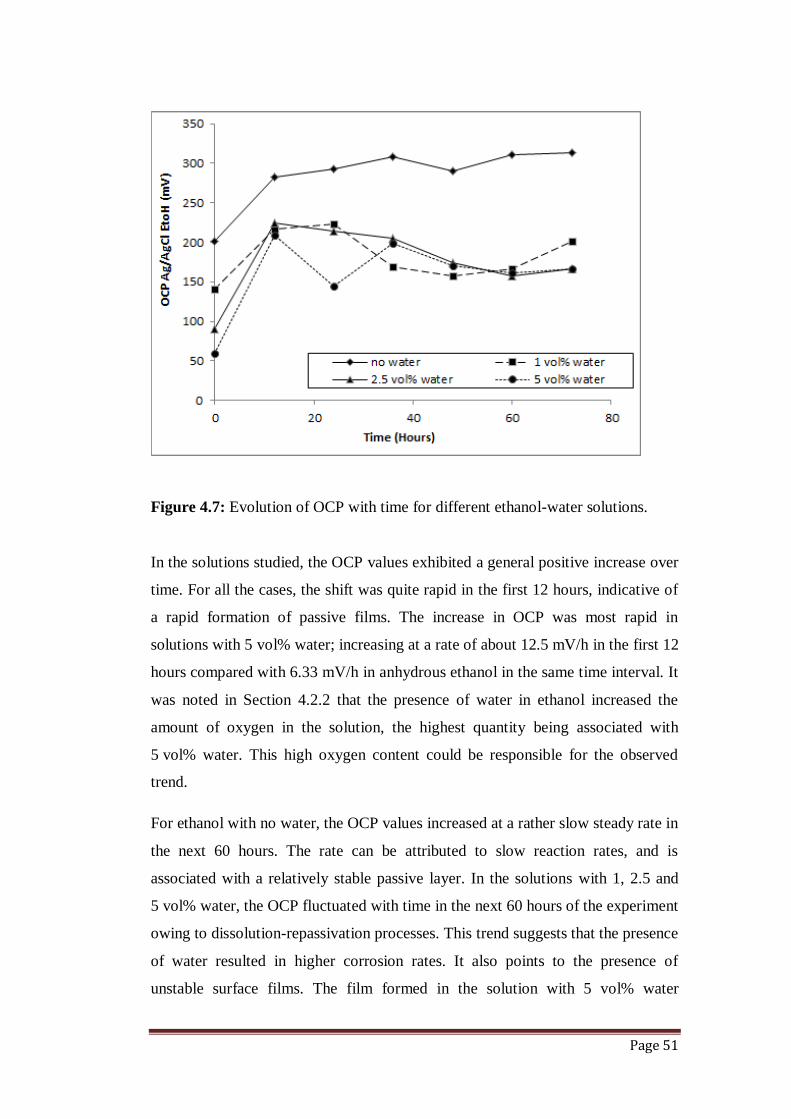
Page 51
Figure 4.7: Evolution of OCP with time for different ethanol-water solutions.
In the solutions studied, the OCP values exhibited a general positive increase over
time. For all the cases, the shift was quite rapid in the first 12 hours, indicative of
a rapid formation of passive films. The increase in OCP was most rapid in
solutions with 5 vol% water; increasing at a rate of about 12.5 mV/h in the first 12
hours compared with 6.33 mV/h in anhydrous ethanol in the same time interval. It
was noted in Section 4.2.2 that the presence of water in ethanol increased the
amount of oxygen in the solution, the highest quantity being associated with
5 vol% water. This high oxygen content could be responsible for the observed
trend.
For ethanol with no water, the OCP values increased at a rather slow steady rate in
the next 60 hours. The rate can be attributed to slow reaction rates, and is
associated with a relatively stable passive layer. In the solutions with 1, 2.5 and
5 vol% water, the OCP fluctuated with time in the next 60 hours of the experiment
owing to dissolution-repassivation processes. This trend suggests that the presence
of water resulted in higher corrosion rates. It also points to the presence of
unstable surface films. The film formed in the solution with 5 vol% water
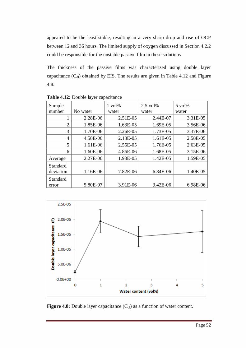
Page 52
appeared to be the least stable, resulting in a very sharp drop and rise of OCP
between 12 and 36 hours. The limited supply of oxygen discussed in Section 4.2.2
could be responsible for the unstable passive film in these solutions.
The thickness of the passive films was characterized using double layer
capacitance (Cdl) obtained by EIS. The results are given in Table 4.12 and Figure
4.8.
Table 4.12: Double layer capacitance
Sample
number No water
1 vol%
water
2.5 vol%
water
5 vol%
water
1 2.28E-06 2.51E-05 2.44E-07 3.31E-05
2 1.85E-06 1.63E-05 1.69E-05 3.56E-06
3 1.70E-06 2.26E-05 1.73E-05 3.37E-06
4 4.58E-06 2.13E-05 1.61E-05 2.58E-05
5 1.61E-06 2.56E-05 1.76E-05 2.63E-05
6 1.60E-06 4.86E-06 1.68E-05 3.15E-06
Average 2.27E-06 1.93E-05 1.42E-05 1.59E-05
Standard
deviation 1.16E-06 7.82E-06 6.84E-06 1.40E-05
Standard
error 5.80E-07 3.91E-06 3.42E-06 6.98E-06
Figure 4.8: Double layer capacitance (Cdl) as a function of water content.
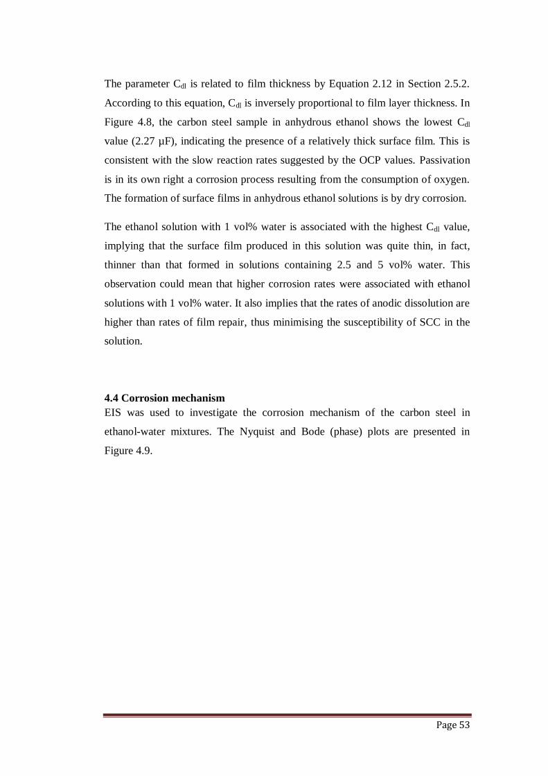
Page 53
The parameter Cdl is related to film thickness by Equation 2.12 in Section 2.5.2.
According to this equation, Cdl is inversely proportional to film layer thickness. In
Figure 4.8, the carbon steel sample in anhydrous ethanol shows the lowest Cdl
value (2.27 µF), indicating the presence of a relatively thick surface film. This is
consistent with the slow reaction rates suggested by the OCP values. Passivation
is in its own right a corrosion process resulting from the consumption of oxygen.
The formation of surface films in anhydrous ethanol solutions is by dry corrosion.
The ethanol solution with 1 vol% water is associated with the highest Cdl value,
implying that the surface film produced in this solution was quite thin, in fact,
thinner than that formed in solutions containing 2.5 and 5 vol% water. This
observation could mean that higher corrosion rates were associated with ethanol
solutions with 1 vol% water. It also implies that the rates of anodic dissolution are
higher than rates of film repair, thus minimising the susceptibility of SCC in the
solution.
4.4 Corrosion mechanism
EIS was used to investigate the corrosion mechanism of the carbon steel in
ethanol-water mixtures. The Nyquist and Bode (phase) plots are presented in
Figure 4.9.
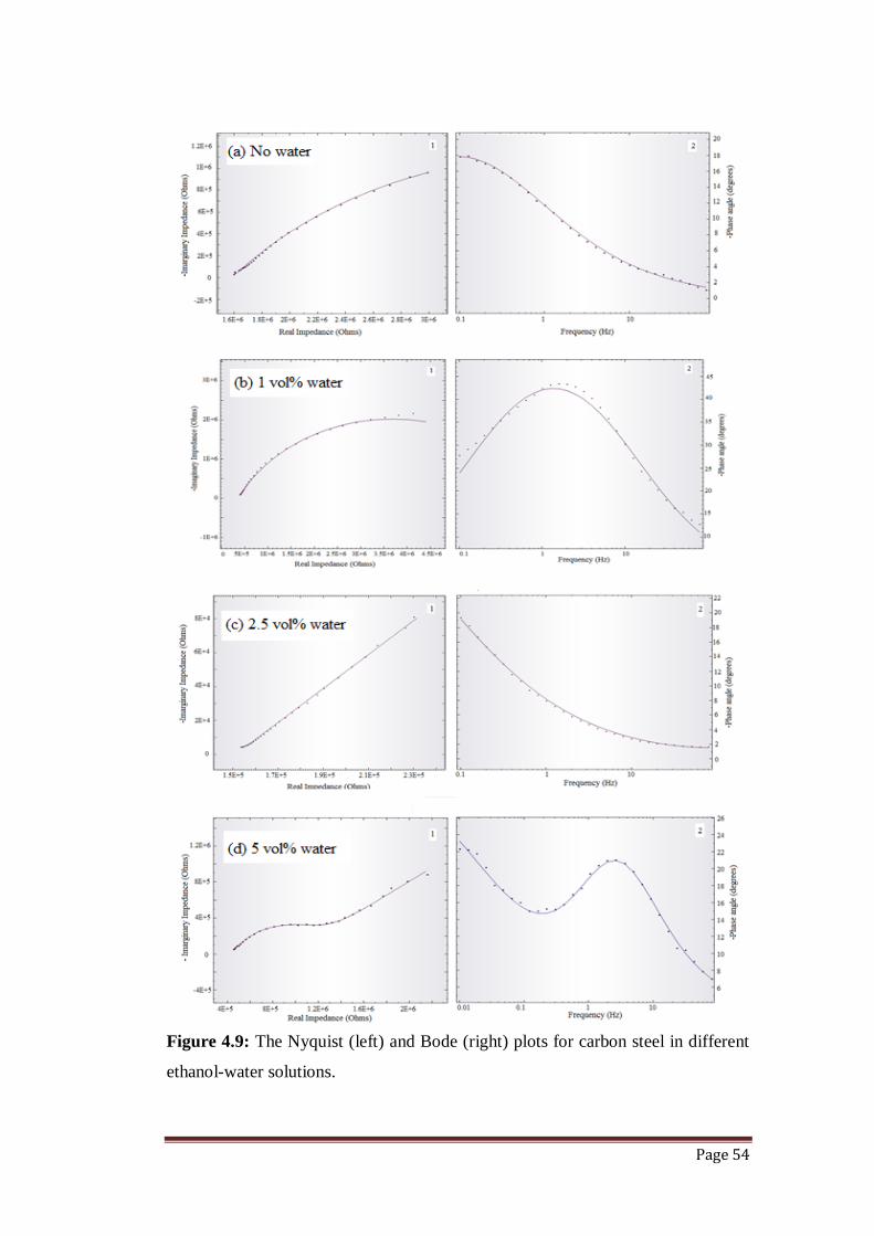
Page 54
Figure 4.9: The Nyquist (left) and Bode (right) plots for carbon steel in different
ethanol-water solutions.
Page 55
The Nyquist plot in the ethanol solution containing no water (Figure 4.9 (a))
shows the beginning of a semicircle, indicating a reaction sequence that is charge
transfer controlled. This should be expected, given the high resistivity associated
with this solution presented in Figures 4.1 and 4.2. The semicircle appears to have
a considerably large radius, implying a large value for the polarisation resistance.
Polarisation resistance is due to the formation of insoluble protective films
(Codd et al., 1970) and a large resistance is indicative of negligible corrosion
rates.
In the solution with 1 vol% water, the Nyquist plot, Figure 4.9 (b), is also a
semicircle but with a smaller radius, suggesting higher corrosion rates. While the
Nyquist plot suggests a charge transfer controlled reaction sequence, the Bode
plot (Figure 4.9 (b) right) indicates a corrosion process under mixed control. The
corrosion process is not only dependent on the resistivity of the solution, but also
on the mass transport of oxygen to the corrosion surface. This is consistent with
the suggestion made in Section 2.2.2 that the presence of water in ethanol
markedly reduces the diffusion rate of oxygen in the reaction surface.
An increase in water content to 2.5 vol% changes the shape of the Nyquist plot
(Figure 4.9 (c)) to a straight line with a slope of about 0.93. The shape of the plot
means that the corrosion reaction in the solution is diffusion-controlled. The
Warburg impedance, represented by the slope of the plot is almost one, indicating
active corrosion.
The Nyquist plot in Figure 4.9(d) shows a depressed semi-circle at high
frequencies and a straight line at low frequencies, indicating a corrosion process
that is under mixed control: charge transfer at high frequencies and diffusion at
low frequencies. The depression on the circle could be due to a lack of
homogeneity of the electrode surface, perhaps inhomogeneity brought about by
local attack.
Post-test examination, by use of a stereomicroscope, was used to confirm the
suggested corrosion mechanisms. Figure 4.10 presents the results of the visual
inspection of the carbon steel specimens exposed to the different ethanol-water

Page 56
mixtures for 72 hours. The corroded samples were compared to an un-etched un-
corroded baseline sample (Figure 4.10(a)).
Figure 4.10: Micrographs of the carbon steel after 72 hours of immersion.
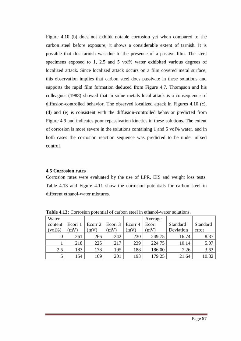
Page 57
Figure 4.10 (b) does not exhibit notable corrosion yet when compared to the
carbon steel before exposure; it shows a considerable extent of tarnish. It is
possible that this tarnish was due to the presence of a passive film. The steel
specimens exposed to 1, 2.5 and 5 vol% water exhibited various degrees of
localized attack. Since localized attack occurs on a film covered metal surface,
this observation implies that carbon steel does passivate in these solutions and
supports the rapid film formation deduced from Figure 4.7. Thompson and his
colleagues (1988) showed that in some metals local attack is a consequence of
diffusion-controlled behavior. The observed localized attack in Figures 4.10 (c),
(d) and (e) is consistent with the diffusion-controlled behavior predicted from
Figure 4.9 and indicates poor repassivation kinetics in these solutions. The extent
of corrosion is more severe in the solutions containing 1 and 5 vol% water, and in
both cases the corrosion reaction sequence was predicted to be under mixed
control.
4.5 Corrosion rates
Corrosion rates were evaluated by the use of LPR, EIS and weight loss tests.
Table 4.13 and Figure 4.11 show the corrosion potentials for carbon steel in
different ethanol-water mixtures.
Table 4.13: Corrosion potential of carbon steel in ethanol-water solutions.
Water
content
(vol%)
Ecorr 1
(mV)
Ecorr 2
(mV)
Ecorr 3
(mV)
Ecorr 4
(mV)
Average
Ecorr
(mV)
Standard
Deviation
Standard
error
0 261 266 242 230 249.75 16.74 8.37
1 218 225 217 239 224.75 10.14 5.07
2.5 183 178 195 188 186.00 7.26 3.63
5 154 169 201 193 179.25 21.64 10.82
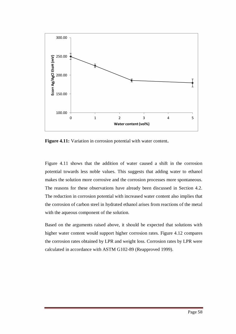
Page 58
Figure 4.11: Variation in corrosion potential with water content.
Figure 4.11 shows that the addition of water caused a shift in the corrosion
potential towards less noble values. This suggests that adding water to ethanol
makes the solution more corrosive and the corrosion processes more spontaneous.
The reasons for these observations have already been discussed in Section 4.2.
The reduction in corrosion potential with increased water content also implies that
the corrosion of carbon steel in hydrated ethanol arises from reactions of the metal
with the aqueous component of the solution.
Based on the arguments raised above, it should be expected that solutions with
higher water content would support higher corrosion rates. Figure 4.12 compares
the corrosion rates obtained by LPR and weight loss. Corrosion rates by LPR were
calculated in accordance with ASTM G102-89 (Reapproved 1999).
100.00
150.00
200.00
250.00
300.00
0 1 2 3 4 5
Eco
rr A
g/A
gCl E
toH
(m
V)
Water content (vol%)
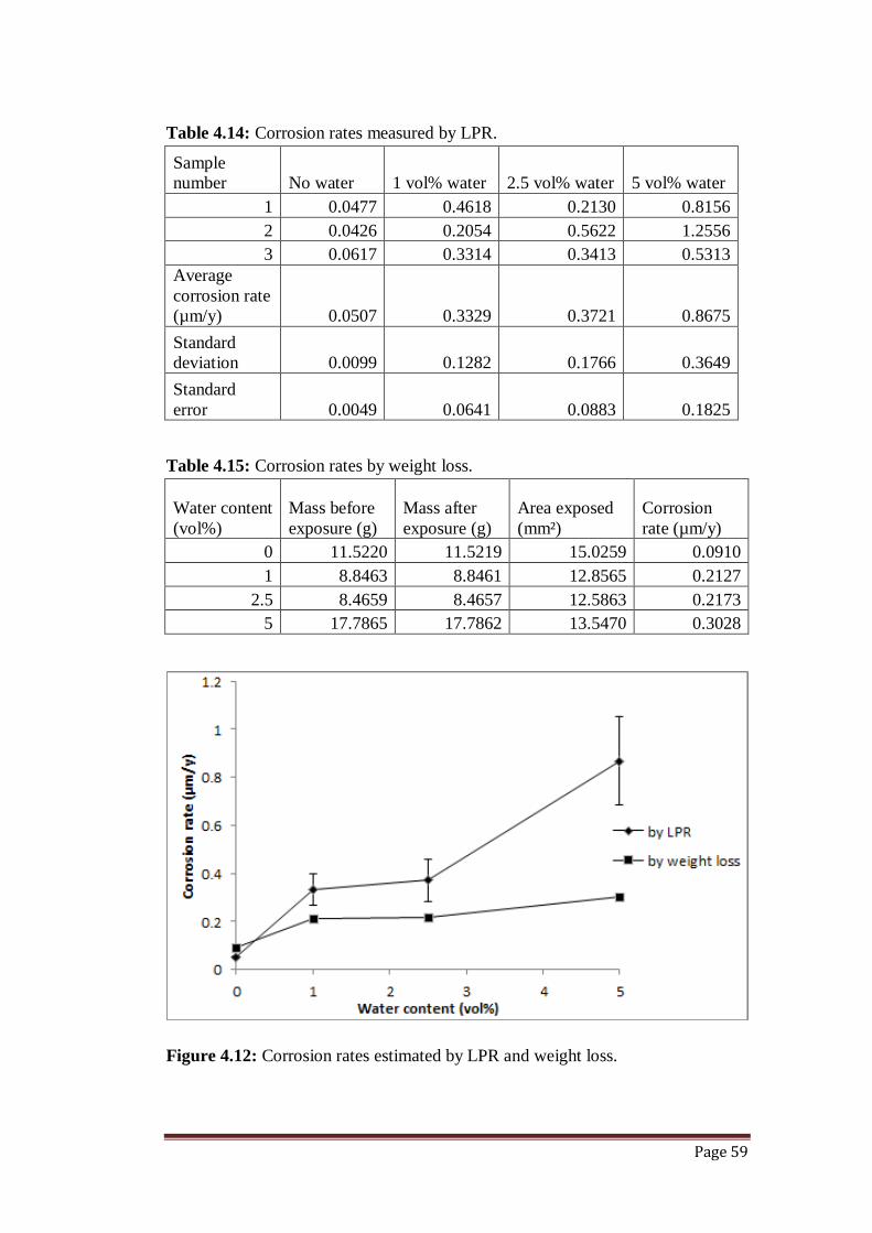
Page 59
Table 4.14: Corrosion rates measured by LPR.
Sample
number No water 1 vol% water 2.5 vol% water 5 vol% water
1 0.0477 0.4618 0.2130 0.8156
2 0.0426 0.2054 0.5622 1.2556
3 0.0617 0.3314 0.3413 0.5313
Average
corrosion rate
(µm/y) 0.0507 0.3329 0.3721 0.8675
Standard
deviation 0.0099 0.1282 0.1766 0.3649
Standard
error 0.0049 0.0641 0.0883 0.1825
Table 4.15: Corrosion rates by weight loss.
Water content
(vol%)
Mass before
exposure (g)
Mass after
exposure (g)
Area exposed
(mm²)
Corrosion
rate (µm/y)
0 11.5220 11.5219 15.0259 0.0910
1 8.8463 8.8461 12.8565 0.2127
2.5 8.4659 8.4657 12.5863 0.2173
5 17.7865 17.7862 13.5470 0.3028
Figure 4.12: Corrosion rates estimated by LPR and weight loss.
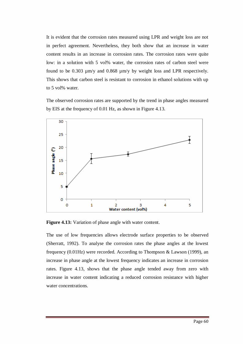
Page 60
It is evident that the corrosion rates measured using LPR and weight loss are not
in perfect agreement. Nevertheless, they both show that an increase in water
content results in an increase in corrosion rates. The corrosion rates were quite
low: in a solution with 5 vol% water, the corrosion rates of carbon steel were
found to be 0.303 µm/y and 0.868 µm/y by weight loss and LPR respectively.
This shows that carbon steel is resistant to corrosion in ethanol solutions with up
to 5 vol% water.
The observed corrosion rates are supported by the trend in phase angles measured
by EIS at the frequency of 0.01 Hz, as shown in Figure 4.13.
Figure 4.13: Variation of phase angle with water content.
The use of low frequencies allows electrode surface properties to be observed
(Sherratt, 1992). To analyse the corrosion rates the phase angles at the lowest
frequency (0.01Hz) were recorded. According to Thompson & Lawson (1999), an
increase in phase angle at the lowest frequency indicates an increase in corrosion
rates. Figure 4.13, shows that the phase angle tended away from zero with
increase in water content indicating a reduced corrosion resistance with higher
water concentrations.
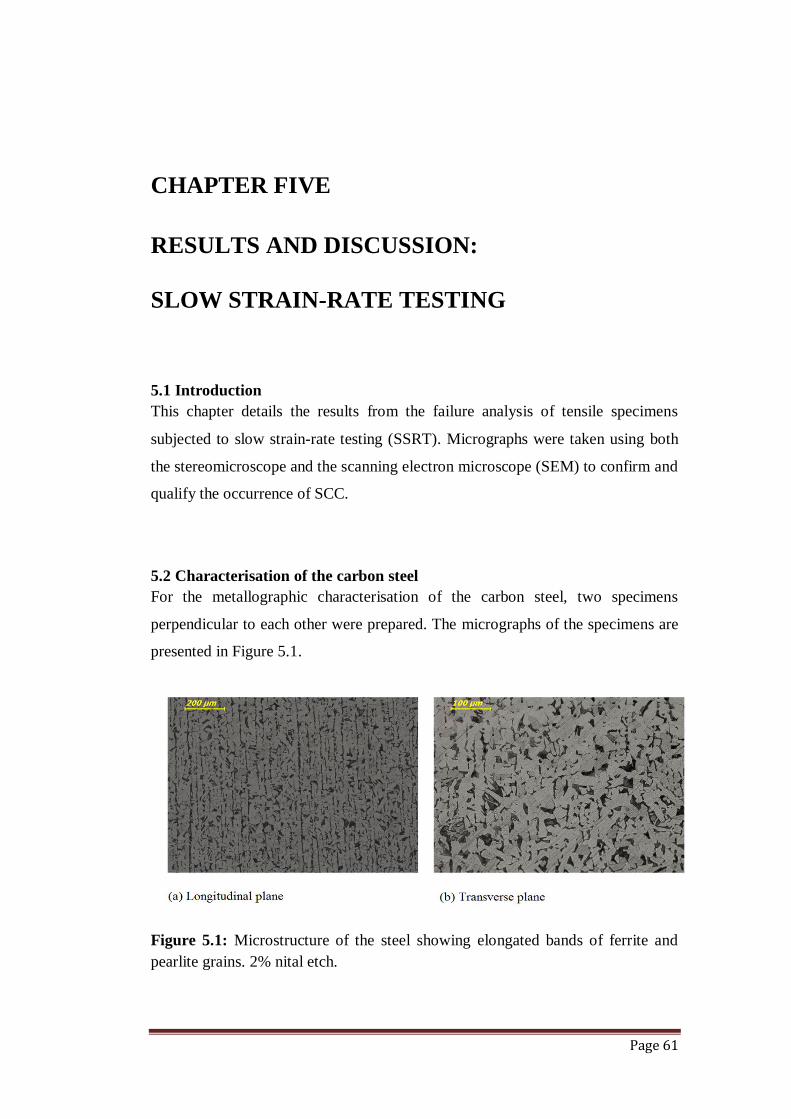
Page 61
CHAPTER FIVE
RESULTS AND DISCUSSION:
SLOW STRAIN-RATE TESTING
5.1 Introduction
This chapter details the results from the failure analysis of tensile specimens
subjected to slow strain-rate testing (SSRT). Micrographs were taken using both
the stereomicroscope and the scanning electron microscope (SEM) to confirm and
qualify the occurrence of SCC.
5.2 Characterisation of the carbon steel
For the metallographic characterisation of the carbon steel, two specimens
perpendicular to each other were prepared. The micrographs of the specimens are
presented in Figure 5.1.
Figure 5.1: Microstructure of the steel showing elongated bands of ferrite and
pearlite grains. 2% nital etch.
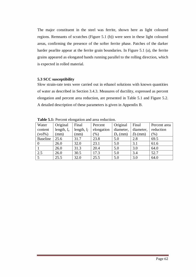
Page 62
The major constituent in the steel was ferrite, shown here as light coloured
regions. Remnants of scratches (Figure 5.1 (b)) were seen in these light coloured
areas, confirming the presence of the softer ferrite phase. Patches of the darker
harder pearlite appear at the ferrite grain boundaries. In Figure 5.1 (a), the ferrite
grains appeared as elongated bands running parallel to the rolling direction, which
is expected in rolled material.
5.3 SCC susceptibility
Slow strain-rate tests were carried out in ethanol solutions with known quantities
of water as described in Section 3.4.3. Measures of ductility, expressed as percent
elongation and percent area reduction, are presented in Table 5.1 and Figure 5.2.
A detailed description of these parameters is given in Appendix B.
Table 5.1: Percent elongation and area reduction.
Water
content
(vol%)
Original
length, lo
(mm)
Final
length, lf
(mm)
Percent
elongation
(%)
Original
diameter,
Do (mm)
Final
diameter,
Df (mm)
Percent area
reduction
(%)
Baseline 25.6 31.7 23.8 5.0 2.8 69.5
0 26.0 32.0 23.1 5.0 3.1 61.6
1 26.0 31.3 20.4 5.0 3.0 64.0
2.5 26.0 30.5 17.3 5.0 3.4 52.7
5 25.5 32.0 25.5 5.0 3.0 64.0
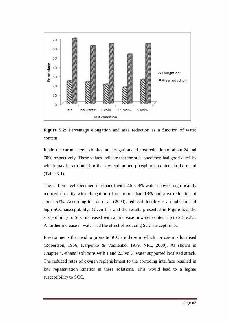
Page 63
Figure 5.2: Percentage elongation and area reduction as a function of water
content.
In air, the carbon steel exhibited an elongation and area reduction of about 24 and
70% respectively. These values indicate that the steel specimen had good ductility
which may be attributed to the low carbon and phosphorus content in the metal
(Table 3.1).
The carbon steel specimen in ethanol with 2.5 vol% water showed significantly
reduced ductility with elongation of not more than 18% and area reduction of
about 53%. According to Lou et al. (2009), reduced ductility is an indication of
high SCC susceptibility. Given this and the results presented in Figure 5.2, the
susceptibility to SCC increased with an increase in water content up to 2.5 vol%.
A further increase in water had the effect of reducing SCC susceptibility.
Environments that tend to promote SCC are those in which corrosion is localised
(Robertson, 1956; Karpenko & Vasilenko, 1979; NPL, 2000). As shown in
Chapter 4, ethanol solutions with 1 and 2.5 vol% water supported localised attack.
The reduced rates of oxygen replenishment to the corroding interface resulted in
low repassivation kinetics in these solutions. This would lead to a higher
susceptibility to SCC.
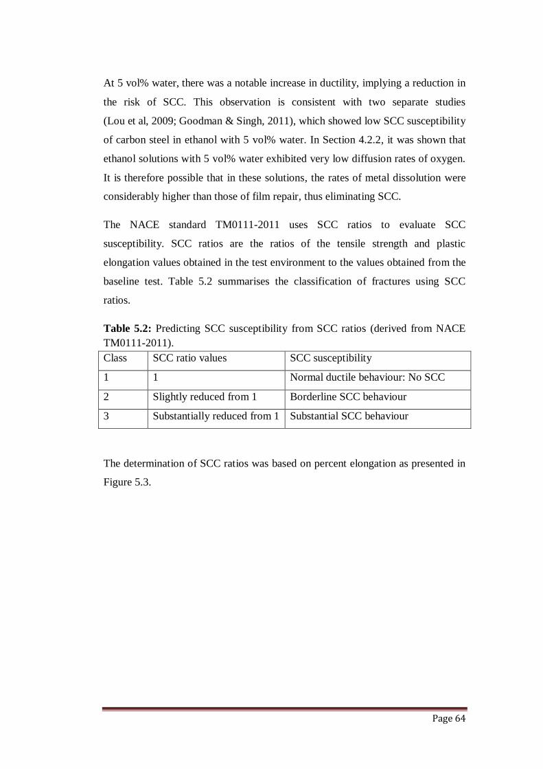
Page 64
At 5 vol% water, there was a notable increase in ductility, implying a reduction in
the risk of SCC. This observation is consistent with two separate studies
(Lou et al, 2009; Goodman & Singh, 2011), which showed low SCC susceptibility
of carbon steel in ethanol with 5 vol% water. In Section 4.2.2, it was shown that
ethanol solutions with 5 vol% water exhibited very low diffusion rates of oxygen.
It is therefore possible that in these solutions, the rates of metal dissolution were
considerably higher than those of film repair, thus eliminating SCC.
The NACE standard TM0111-2011 uses SCC ratios to evaluate SCC
susceptibility. SCC ratios are the ratios of the tensile strength and plastic
elongation values obtained in the test environment to the values obtained from the
baseline test. Table 5.2 summarises the classification of fractures using SCC
ratios.
Table 5.2: Predicting SCC susceptibility from SCC ratios (derived from NACE
TM0111-2011).
Class SCC ratio values SCC susceptibility
1 1 Normal ductile behaviour: No SCC
2 Slightly reduced from 1 Borderline SCC behaviour
3 Substantially reduced from 1 Substantial SCC behaviour
The determination of SCC ratios was based on percent elongation as presented in
Figure 5.3.
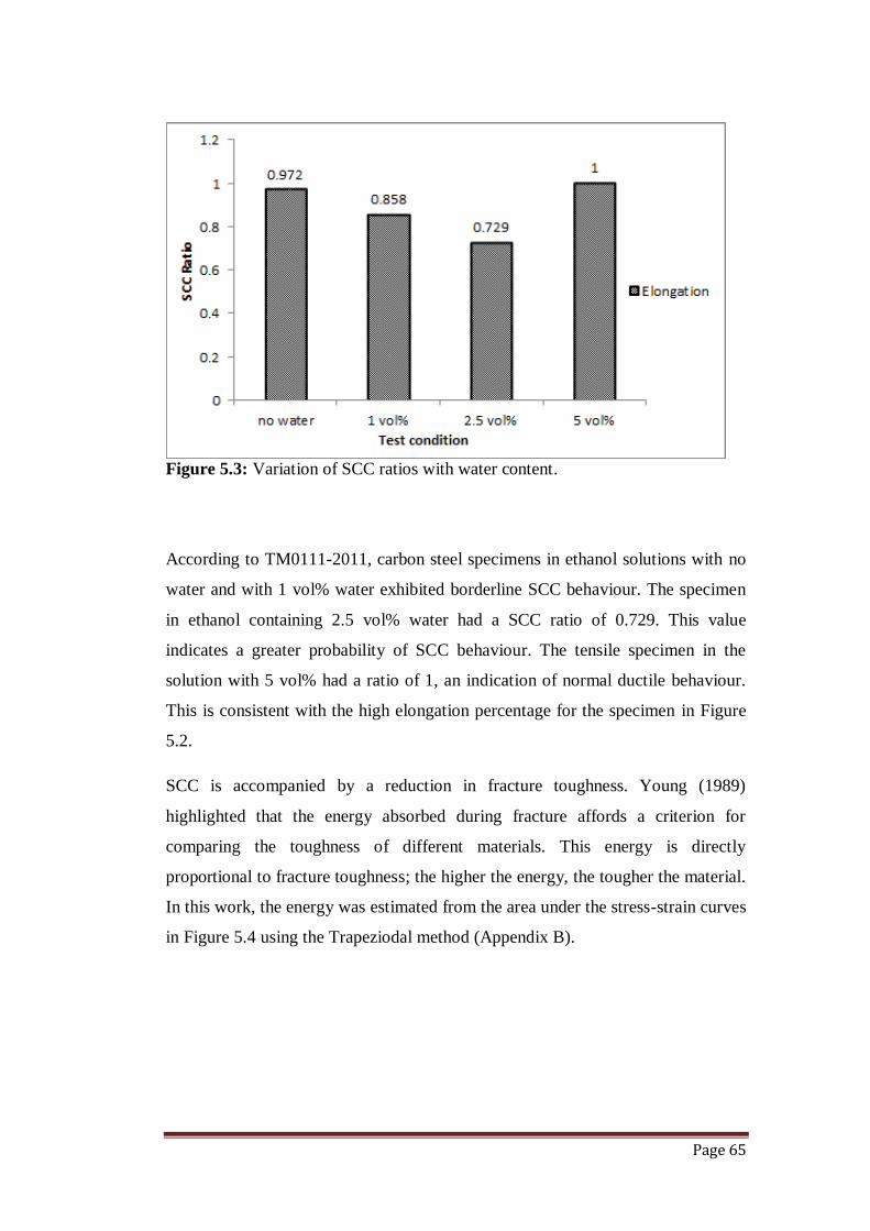
Page 65
Figure 5.3: Variation of SCC ratios with water content.
According to TM0111-2011, carbon steel specimens in ethanol solutions with no
water and with 1 vol% water exhibited borderline SCC behaviour. The specimen
in ethanol containing 2.5 vol% water had a SCC ratio of 0.729. This value
indicates a greater probability of SCC behaviour. The tensile specimen in the
solution with 5 vol% had a ratio of 1, an indication of normal ductile behaviour.
This is consistent with the high elongation percentage for the specimen in Figure
5.2.
SCC is accompanied by a reduction in fracture toughness. Young (1989)
highlighted that the energy absorbed during fracture affords a criterion for
comparing the toughness of different materials. This energy is directly
proportional to fracture toughness; the higher the energy, the tougher the material.
In this work, the energy was estimated from the area under the stress-strain curves
in Figure 5.4 using the Trapeziodal method (Appendix B).
Page 66
Figure 5.4: Stress-strain curves for the carbon steel specimens in different
ethanol-water mixtures. (a) baseline, (b) no water, (c) 1 vol% water, (d) 2.5 vol%
water and (e) 5 vol% water.
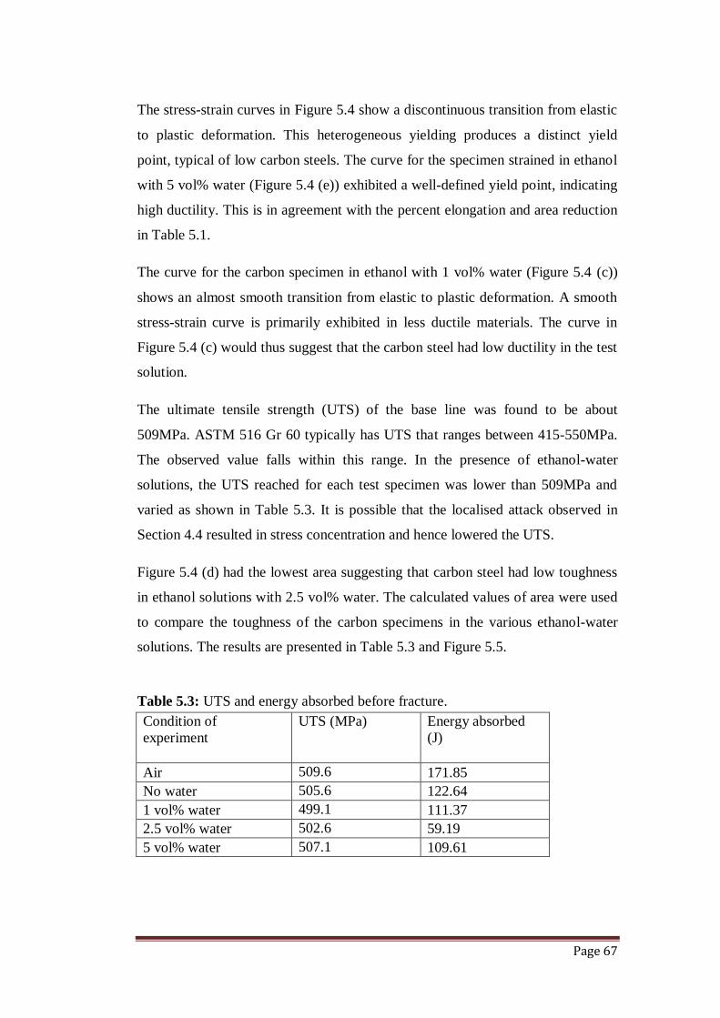
Page 67
The stress-strain curves in Figure 5.4 show a discontinuous transition from elastic
to plastic deformation. This heterogeneous yielding produces a distinct yield
point, typical of low carbon steels. The curve for the specimen strained in ethanol
with 5 vol% water (Figure 5.4 (e)) exhibited a well-defined yield point, indicating
high ductility. This is in agreement with the percent elongation and area reduction
in Table 5.1.
The curve for the carbon specimen in ethanol with 1 vol% water (Figure 5.4 (c))
shows an almost smooth transition from elastic to plastic deformation. A smooth
stress-strain curve is primarily exhibited in less ductile materials. The curve in
Figure 5.4 (c) would thus suggest that the carbon steel had low ductility in the test
solution.
The ultimate tensile strength (UTS) of the base line was found to be about
509MPa. ASTM 516 Gr 60 typically has UTS that ranges between 415-550MPa.
The observed value falls within this range. In the presence of ethanol-water
solutions, the UTS reached for each test specimen was lower than 509MPa and
varied as shown in Table 5.3. It is possible that the localised attack observed in
Section 4.4 resulted in stress concentration and hence lowered the UTS.
Figure 5.4 (d) had the lowest area suggesting that carbon steel had low toughness
in ethanol solutions with 2.5 vol% water. The calculated values of area were used
to compare the toughness of the carbon specimens in the various ethanol-water
solutions. The results are presented in Table 5.3 and Figure 5.5.
Table 5.3: UTS and energy absorbed before fracture.
Condition of
experiment
UTS (MPa) Energy absorbed
(J)
Air 509.6 171.85
No water 505.6 122.64
1 vol% water 499.1 111.37
2.5 vol% water 502.6 59.19
5 vol% water 507.1 109.61
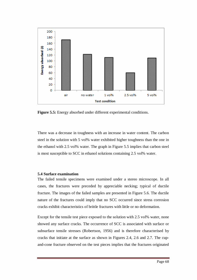
Page 68
Figure 5.5: Energy absorbed under different experimental conditions.
There was a decrease in toughness with an increase in water content. The carbon
steel in the solution with 5 vol% water exhibited higher toughness than the one in
the ethanol with 2.5 vol% water. The graph in Figure 5.5 implies that carbon steel
is most susceptible to SCC in ethanol solutions containing 2.5 vol% water.
5.4 Surface examination
The failed tensile specimens were examined under a stereo microscope. In all
cases, the fractures were preceded by appreciable necking; typical of ductile
fracture. The images of the failed samples are presented in Figure 5.6. The ductile
nature of the fractures could imply that no SCC occurred since stress corrosion
cracks exhibit characteristics of brittle fractures with little or no deformation.
Except for the tensile test piece exposed to the solution with 2.5 vol% water, none
showed any surface cracks. The occurrence of SCC is associated with surface or
subsurface tensile stresses (Robertson, 1956) and is therefore characterised by
cracks that initiate at the surface as shown in Figures 2.4, 2.6 and 2.7. The cup-
and-cone fracture observed on the test pieces implies that the fractures originated
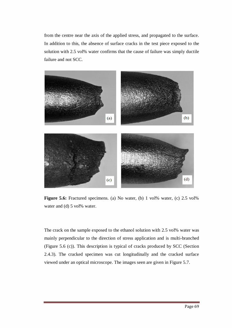
Page 69
from the centre near the axis of the applied stress, and propagated to the surface.
In addition to this, the absence of surface cracks in the test piece exposed to the
solution with 2.5 vol% water confirms that the cause of failure was simply ductile
failure and not SCC.
Figure 5.6: Fractured specimens. (a) No water, (b) 1 vol% water, (c) 2.5 vol%
water and (d) 5 vol% water.
The crack on the sample exposed to the ethanol solution with 2.5 vol% water was
mainly perpendicular to the direction of stress application and is multi-branched
(Figure 5.6 (c)). This description is typical of cracks produced by SCC (Section
2.4.3). The cracked specimen was cut longitudinally and the cracked surface
viewed under an optical microscope. The images seen are given in Figure 5.7.
Page 70
Figure 5.7: Surface cracks (indicated by arrows) on the carbon specimen viewed
at different angles. 2% nital.
The cracks cut across the ferrite and pearlite grains, typical of TG-SCC
(Figure 2.6). The average crack length was found to be 60.34 μm. Dividing the
crack length by the time to failure gave a crack velocity of about 2.66x10⁻7 mm/s.
This value is much greater than that observed by Lou (2010) (Figure 2.8).
SEM fractographs were obtained to study the crack on the test piece in the ethanol
solution with 2.5 vol% water. The SEM fractographs are shown in Figure 5.8. The
crack is multi-branched, as observed under the stereomicroscope.
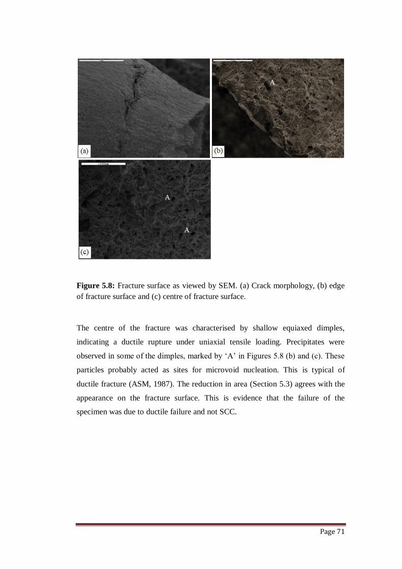
Page 71
Figure 5.8: Fracture surface as viewed by SEM. (a) Crack morphology, (b) edge
of fracture surface and (c) centre of fracture surface.
The centre of the fracture was characterised by shallow equiaxed dimples,
indicating a ductile rupture under uniaxial tensile loading. Precipitates were
observed in some of the dimples, marked by ‘A’ in Figures 5.8 (b) and (c). These
particles probably acted as sites for microvoid nucleation. This is typical of
ductile fracture (ASM, 1987). The reduction in area (Section 5.3) agrees with the
appearance on the fracture surface. This is evidence that the failure of the
specimen was due to ductile failure and not SCC.
Page 72
CHAPTER SIX
CONCLUSIONS
The effects of water on the SCC of carbon steel in ethanolic media were studied
by investigating how it influences the chemical properties of ethanol, the
corrosion characteristics of carbon steel in ethanol-water mixtures and the tensile
properties of carbon steel exposed to different ethanol-water mixtures.
The solution characterisation of ethanol-water revealed that adding water to
ethanol increased oxygen content and the electrical conductivity but did not show
any effect on the acidity of ethanol. The ethanol-water solutions exposed to
carbon steel for short period of time did not show any measurable change in water
content. However, exposure for longer period showed significant changes,
indicating that the degradation of ethanol was time dependent.
The increase in conductivity and oxygen content was accompanied by an increase
in the corrosiveness of ethanol as observed by the increase in corrosion rate in
anhydrous ethanol with increase in water content. The corrosion mechanism of
carbon steel was found to be charge transfer controlled in anhydrous ethanol,
mixed in ethanol with 1 vol% and 5 vol% water and diffusion-controlled in
solutions with 2.5 vol% water.
Despite the high oxygen quantities associated with ethanol solutions containing
higher levels of water, corrosion in these solutions was seen to be characterised by
low diffusion rates of oxygen to the corroding surface, leading to poor
repassivation kinetics. The low diffusion rates implied mean that adding water to
ethanol reduces the diffusion of oxygen in the solution, making it less prone to
promote stable surface films. This was confirmed by the localised attack observed

Page 73
on the corrosion specimens. The extent of attack was more severe in solutions
with 1 and 5 vol% water.
The specimens subjected to SSRT were fairly ductile, exhibiting appreciable
plastic deformation before fracture. The specimen in the ethanol solution with
2.5 vol% water displayed surface cracks perpendicular to the direction of stress
application and satisfied the conditions of the NACE TM0111-2011 criterion for
substantial SCC behaviour. However, the SEM fractographs revealed that the
specimen in this solution had failed by ductile failure and not SCC. The
specimens in solutions containing 0, 1 and 5 vol% water did not exhibit any SCC
characteristics.
This work revealed that while the presence of water in ethanol enabled the
initiation of various extents of corrosion, water contents of up to 5 vol% have no
effect on the SCC susceptibility of carbon steel in ethanolic media.
Recommendations
Strain rate plays a significant role in the SCC of a metal in a given environment
(Shier et al., 1994; Jarvis, 1994). It is recommended that further study be done
using different strain rates to see if the conclusions drawn in this present work
hold at any strain rate.
Page 74
REFERENCES
Agarwal, A.K., 2007, ‘Biofuels (alcohols and biodiesel) applications as fuels for
internal combustion engines’, Progress in Energy and Combustion Science, vol.
33, pp. 233-271.
Arup, H. & Parkins, R.N. (Ed.) 1975, Stress corrosion research, Nato Advanced
Study Institute, Netherlands.
ASM, 1987, ASM Handbook Vol. 12: Fractography, 9th Edn., ASM International,
Ohio, USA.
ASTM D6423 (2008), ‘Standard test method for determination of phe of ethanol,
denatured fuel ethanol, and fuel ethanol (Ed75-Ed85)’, ASTM, West
Conshohocken, USA.
ASTM G3-89 (2010), ‘Standard practise for conventions applicable to
electrochemical measurements corrosion testing’, ASTM, West Conshohocken,
USA.
ASTM G102 (1989) (Reapproved 1999), ‘Standard practise for calculation of
corrosion rates and related information from electrochemical measurements’,
ASTM, West Conshohocken, USA.
Beavers, J.A., Brogers, M.P., Agrawal, A.K. and Tallarida, F.A., 2008,
‘Prevention of internal SCC in ethanol pipelines’, Paper no. 08153, NACE
Corrosion Conference & Expo 2008, accessed on 23 November 2011,
http://www.dnvcolumbus.com/files/dsp_recent_publications_9_1_6.pdf
Bhola, S.M., Bhola, R., Jain, L., Mishra, B. and Olson, D.L., Corrosion behaviour
of mild carbon steel in ethanolic solutions, Journal of Materials Engineering and
Performance, vol. 20, no. 3, pp. 409-416.
Bio-Logic, 2011, Atlas of electrochemical nyquist diagrams: a guide to selected
equivalent circuits, accessed 4 July 2012, www.bio-logic.info
Blue, G.D. and Moran, C.M., 1990, Electrochemical corrosion studies in low
conductivity media, Astronautics Laboratory (AFSC), USA.
Brossia, C.S., 1995, ‘The electrochemistry of iron in methanolic solutions and its
relationship to corrosion’, Corrosion Science, vol. 37, no. 9, pp. 1455-147.
Brown, B.F., 1977, Stress Corrosion Cracking Control Measures, Department of
Commerce, National Bureau of Standards, Washington DC, USA.
Page 75
Clubley, B.G. (Ed.), 1988, Chemical inhibitors for corrosion control, Royal
Society of Chemistry, Manchester, UK, pp. 6, 73.
Codd, L.W., Dijkhoff, K., Fearon, J.H., Van Oss, C.J., Robernsen, H.C., and
Stanford E.G. (Eds.), 1972, Petroleum and Organic Chemicals, Materials and
Technology, vol. 4, Longman, USA, pp. 276-277.
Codd, L.W., Dijkhoff, K., Fearon, J.H., Van Oss, C.J., Robernsen, H.C., Stanford
E.G. and Van Thoor, T.J.W. (Eds.), 1970, Metals and Ores, Materials and
Technology, vol. 3, Longman, USA, pp. 791-795.
de Anna, P.L., 1985, The effects of water and chloride ions on the electrical
behaviour of iron and 304L stainless steel in alcohols, Corrosion science, vol. 25,
no. 1, pp. 43-53.
De Souza, J.P., Mattos, O.R., Sathler, L., Takenont, H., 1987, Impedance
measurements of corroding mild steel in an automotive fuel ethanol with and
without inhibitor in a two and three electrode cell, Corrosion Science, vol. 21, no.
21, pp. 1351-1364.
Ebrahim, N., Momeni, M., Kosari, A., Zakeri, M., and Moayed, M.H., 2012,
‘Comparative study of critical pitting temperature (CPT) of stainless steels by
electrochemical impedance spectroscopy (EIS), potentiodynamic and
potentiostatic techniques’, Corrosion Science, vol. 59, pp. 96-102.
Faraji, M., Farajtabar, A. and Gharib, F., 2009, ‘Determination of water-ethanol
mixtures autoprotolysis constants and solvent effects’, Journal of Applied
Chemical Research, vol. 9, pp. 7-12.
Fergusson, A., 2001, Ozone depletion and climate change: Understanding the
linkages, Ministry of Public Works and Government Services, Canada, accessed
on 26 December 2012, http://expstudies.tor.gc.ca/e/ozone
Fontana, M.G., 1986, Corrosion Engineering, 3rd
Edn, McGraw-Hill, New York,
USA.
Goodman, L. and Singh P.M., 2010, ‘Effects of ethanol fuel on chemistry on SCC
and passivation of pipeline steel’, accessed on 23 November 2011,
http://www.ipst.gatech.edu/students/posters/110309_goodman.pdf
Greene, N.D., 1965, Electrode Kinetics, Rensselaer Polytechnic Institute, New
York, USA.
Herald, Sept 2012, SA introduces mandatory ethanol blending, New Ziana,
accessed on 4 September 2012, www.zimpapers.co.zw

Page 76
Hetĕnyi, M. (Ed.), 1950, Handbook of Experimental Stress Analysis, John Wiley
& Sons, New York, USA.
HILTI, 2000, Corrosion-Resistant Fastenings, accessed on 4 July 2012,
http://www.us.hilti.com/fstore/holus/LinkFiles/hilti.pdf
Jarvis, A.R., 1994, Environmental assisted cracking (EAC) behaviour of a low
alloy nickel in a sour environment, MSc Dissertation, University of the
Witwatersrand, Johannesburg.
Kane, R.D., Maldonado, J.G. and Klein L.J., 2004, ‘Stress corrosion cracking in
fuel ethanol: A newly found phenomenon’, Paper no.04543, Corrosion 2004,
accessed on 23 November 2011,
http://www.icorr.net/wpcontent/uploads/2011/01/Ethanol_SCC.pdf
Karpenko, G.V. and Vasilenko, I.I., 1979, Stress Corrosion Cracking of Steels,
Transtech Publication, Switzerland.
Khuri, A.I., 2003, Advanced Calculus with Application in Statistics, 2nd
Edn.,
John Wiley & Sons, New Jersey, USA.
Knott J.F. and Withey P.A., 1993, Fracture Mechanics: Worked Examples, 2nd
Edn., The Institute of Materials, London, UK.
Lapede, D.N., 1978, Dictionary of scientific and technical terms, 2nd
Edn.,
McGraw Hill, New York, USA, pp. 918.
Lou, X., 2010, Stress corrosion cracking and corrosion of carbon steel in
stimulated fuel-grade ethanol, PhD dissertation, Georgia Institute of Technology,
accessed on 23 November, 2011, http://gateway.proquest.com
Lou, X. and Singh, P.M., 2011, ‘Corrosion and pitting behaviour of carbon steel
in simulated fuel-grade ethanol under variations in ethanol chemistry’, accessed
on 3 December 2011, http://www.onepetro.org/mslib/servlet/onepetropreview
Lou, X., Yang, D. and Singh, P.M., 2009, ‘Effects of ethanol chemistry on stress
corrosion cracking of carbon steel in fuel-grade ethanol’, Corrosion, vol. 65,
no.12, pp. 785-796.
Macdonald, J.R., 1992, ‘Impedance spectroscopy’, Annals of Biomedical
Engineering, vol 20, pp. 289-305.
McMurry, J., 2007, Organic Chemistry: A Biological Approach, Thomson Books,
Belmont, California, USA.
Metrohm, 2011, Autolab Application Notes, accessed on 4 July 2012
http://www.ecochemie.nl/export/Homepages/Autolab/download/Applicationnotes
Page 77
Metzge, R.M., 2012, The Physical Chemist’s Toolbox, John Wiley & Sons, New
Jersey, USA.
NACE Standard TM0111-2011, ‘Standard test method: slow strain rate test
method for evaluation of ethanol stress corrosion cracking in carbon steels’,
NACE International, Houston, USA.
Naik, S.N., Vaibhav, V.G., Prasant, K.R. and Ajay, K.D., 2010, Production of first
and second generation biofuels: A comprehensive review, renewable and
sustainable energy reviews, vol. 14, pp. 578-597, accessed on 10 November 2012,
http://efwscientists.com/WordPress/wp-content/
NPL, 2000, Guidelines to good practice in corrosion control: Stress corrosion
cracking, accessed on 17 November 2011, http://www.npl.co.uk
Newman, R.C., 2008, ‘Review and hypothesis for the stress corrosion mechanism
of carbon steels in alcohols’, Corrosion, vol. 64, no.11, p 819-824.
Nygaard, P.V., 2008, Non-destructive electrochemical monitoring of
reinforcement corrosion, PhD Thesis, Technical University of Denmark, accessed
on 8 July 2012,
http://www.byg.dtu.dk/upload/institutter/byg/publications/rapporter/byg-r202.pdf
Obuka, N.S., Okoli, N.C., Ikwu G.R. and Chukwumuanya, E.O., 2012, ‘Review
of corrosion kinetics and thermodynamics of CO2 and H2S corrosion effects and
associated prediction/evaluation on oil and gas pipeline steel’, International
Journal of Scientific and Technology Research, vol. 1, no. 4, p. 156-162.
ORNL, 2008, ‘Ethanol pipeline corrosion literature study: Final report’, accessed
on 23 November 2011, http://www.ornl.gov/sci/ees/itp/documents/ORNL
Osterman, K., 2012, ‘Stainless steels: cost effective materials’, Ethanol Producer
Magazine, accessed on 26 December 2012,
http://ethanolproducer.com/articles/8853/stainless-steels-cost-effective-materials
Perry, R.H. and Green D.W. (Ed.), 1999, Perry’s Chemical Engineers’ Handbook,
7th edn, McGraw-Hill, USA.
Pletcher, D., 1991, A First Course in Electrode Processes, The Electrochemical
Consultancy, England.
REM, 2012, Global ethanol production to top 85billion litres in 2012, Renewable
Energy Magazine, accessed on 29 December 2012,
www.renewableenergymagazine.com/article/global-ethanol-to-top-85-billion
Page 78
Reseder, R.S.T. (Ed.), 1980, NACE Corrosion Engineer’s Reference Book, NACE
International, Houston, USA.
Revie, R.W. (Ed.), 2011, Uhlig’s Corrosion Handbook, John Wiley and Sons,
New Jersey, USA.
RFA, 2012, Accelerating Industry Innovation: 2012 Ethanol Industry Outlook,
accessed on 10 November 2012, http://ethanolrfa.3cdn.net
Rhodin, T.N. (Ed.), 1959, Physical Metallurgy of Stress Corrosion Fracture,
Metallurgical Society Conferences, AIME, Pennsylvania, USA.
Roberge, P.R., 2008, Corrosion Kinetics and Application of Electrochemistry to
Corrosion, McGraw Hill, New York, USA.
Robertson, W.D., 1956, Stress Corrosion Cracking and Embrittlement, John
Wiley, New York, USA.
Roelf, W., 2012, ‘South Africa sees $ 258mln ethanol plant by 2014’, Reuters US
Edition accessed on 3 March 2012,
http://news.yahoo.com/africa-sees-258-mln-ethanol-plant-2014-112718876.html
Rosenblim, L., Scheuermann, C., Barrett, C.A. and Lowdermilk, W.H., 1968,
‘Mechanism and kinetics of corrosion of selected iron and cobalt alloys in
refluxing mercury’, NASA, Washington DC, accessed on 26 December, 2012
http://www.researchgate.net/publication/24334555
Scheel, J., September 2010, ‘Eliminating stress corrosion cracking in stainless
steels’, Metal Finishing News, vol. 11, accessed on 3 March 2012,
http://mfn.li/article/?id=898
Schweitzer, P.A., 2010, Fundamentals of Corrosion: Mechanism, Causes and
Preventative Methods, CRC Press, New York, USA.
Scribner, L.A., 2001, ‘Corrosion by organic acids’, Corrosion, accessed on 17
January 2012, www.onepetro.org/mslib/servlet/onepetropreview
Shier, L.L., Jarman, R.A. and Burstein, G.T., 1994, Corrosion Volume 1: Metals/
Environment Reactions, 3rd
edn, Butterworth Heinemann, Oxford.
Sherratt, M.S., 1992, Corrosion monitoring using electrochemical noise, LPR,
ZRA and AC impedance techniques, MSc Dissertation, University of the
Witwatersrand, Johannesburg, RSA.
Simbi, D.J., 2006, Lecture notes distributed in Corrosion engineering MG415,
University of Zimbabwe, Harare, Zimbabwe, on February 2006.

Page 79
Song, H. and Saraswathy, V., 2007, ‘Corrosion monitoring of the reinforced
concrete structures: A review’, International Journal of Electrochemical Science,
vol. 2, pp. 1-20.
Spitzer, P., Fisicaro, P., Seitz, S. and Champion, R., 2009, ‘pH and the electrolytic
conductivity as parameters to characterize bioethanol’, Accred. Qual. Assur., vol.
14, pp. 617-676, accessed on 3 March 2012, http://link.springer.com/content/pdf
Sridhar, N., Price, K., Buckingham, J. and Dante, J., 2006, ‘Stress corrosion
cracking of carbon steel in ethanol’, Corrosion, vol. 62, no. 8, pp. 687-702.
Stassa, 2012, Census 2011 Statistical Release P0301.4, Statistics South Africa,
Pretoria, accessed on 26 December 2012, www.statssa.gov.za
Tembe, S.M., 2010, Low temperature oxidation of ethanol to acetic acid using
gold based catalysts, MSc Dissertation, University of Witwatersrand,
Johannesburg, RSA.
Thompson, N.G. and Lawson, K.M., 1991, An electrochemical method for
detecting ongoing corrosion of steel in a concrete structure with cathodic
protection applied, Strategic Highway Research Program, National Research
Council, Washington DC, USA.
Thompson, N.G., Lawson, K.M. and Beavers, J.A., 1988, ‘Monitoring
cathodically protected steel in concrete structures with electrochemical impedance
techniques’, Corrosion Engineering, vol. 44, no. 8, pp. 581-588.
Uhlig, H. (Ed.), 1948, Corrosion Handbook, John Wiley & Sons, London.
UN-Energy, 2011, Ethanol Fuel in Brazil, Energy Stories, accessed on 2 January
2013, http://www.un-energy.org/stories/38-ethanol-fuel-in-brazil
Van der Merwe, J.W., 2011, Introduction to corrosion, Lecture notes distributed
in Weldability of steels and stainless steels CHMT7050, University of
Witwatersrand, Johannesburg on 12 September 2011.
Yahalom, J. and Aladjem, A., 1980, Stress Corrosion Cracking, Freund
Publishing House, Israel.
Yates, P., 2005, Chemical Calculations at a Glance, Blackwell Publishing,
England.
Young, W.C., 1989, Roark’s formulas for stress and strain, 6th Edn., McGraw
Hill, UK.
Page 80
APPENDICES
Appendix A
Water content estimation
Apparatus:
oven, funnel, filter paper, crucible, timer, measuring scale.
Procedure:
1. Dry crucible in oven at approximately 100⁰C for at least 5 minutes.
2. Allow the crucible to cool and then measure its mass (m1).
3. Add sodium chloride and weigh (m2).
4. Place the crucible in the oven and dry the salt for about 20 minutes.
5. Allow to cool and weigh (m3). If m3-m2 is less than 0.003 g, proceed.
Otherwise, place in the oven and dry further.
6. Dissolve the salt in 50 mL of the solution whose composition is to be
determined.
7. Shake thoroughly for ±4 minutes.
8. Filter. Place residue in the oven for 45-60 minutes.
9. Weigh a dry crucible (m4).
10. Place dried residue in the dry crucible, allow to cool and weigh (m5)
The mass of the salt that has dissolved is given by [(m3-m1)-(m5-m4)]. The
solubility of sodium chloride is thus expressed as this mass per 50 mL.
Statistical analysis
The t-distribution was used to generate a confidence interval. A total of 15 repeats
were measured for solutions with 60 v% water and the solubility of each was
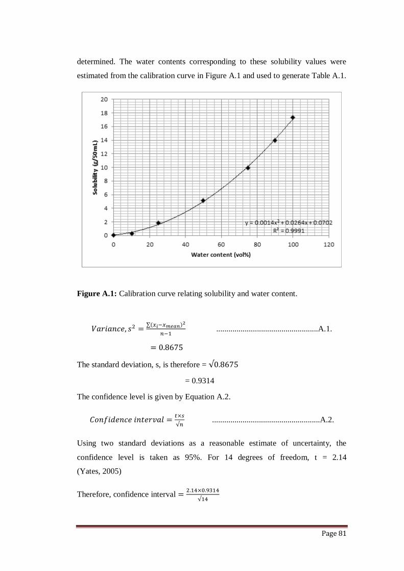
Page 81
determined. The water contents corresponding to these solubility values were
estimated from the calibration curve in Figure A.1 and used to generate Table A.1.
Figure A.1: Calibration curve relating solubility and water content.
∑( )
..................................................A.1.
The standard deviation, s, is therefore =
= 0.9314
The confidence level is given by Equation A.2.
.....................................................A.2.
Using two standard deviations as a reasonable estimate of uncertainty, the
confidence level is taken as 95%. For 14 degrees of freedom, t = 2.14
(Yates, 2005)
Therefore, confidence interval
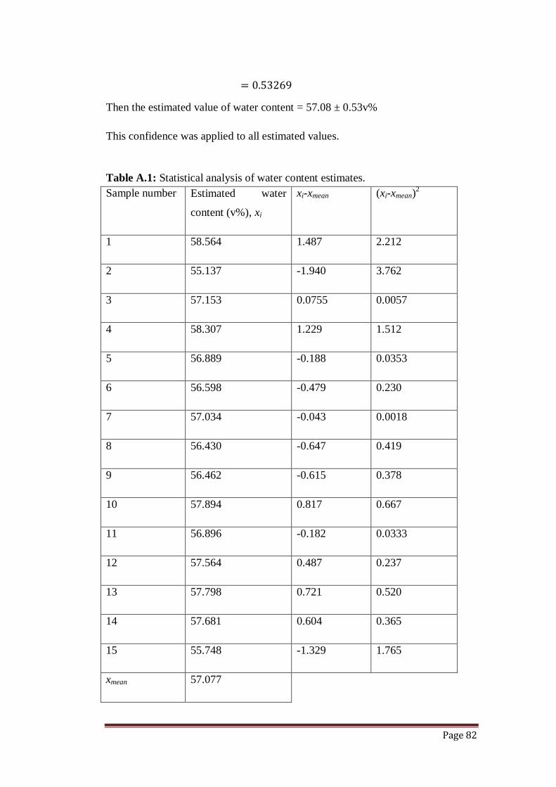
Page 82
Then the estimated value of water content = 57.08 ± 0.53v%
This confidence was applied to all estimated values.
Table A.1: Statistical analysis of water content estimates.
Sample number Estimated water
content (v%), xi
xi-xmean (xi-xmean)2
1 58.564 1.487 2.212
2 55.137 -1.940 3.762
3 57.153 0.0755 0.0057
4 58.307 1.229 1.512
5 56.889 -0.188 0.0353
6 56.598 -0.479 0.230
7 57.034 -0.043 0.0018
8 56.430 -0.647 0.419
9 56.462 -0.615 0.378
10 57.894 0.817 0.667
11 56.896 -0.182 0.0333
12 57.564 0.487 0.237
13 57.798 0.721 0.520
14 57.681 0.604 0.365
15 55.748 -1.329 1.765
xmean 57.077

Page 83
Appendix B
SSRT
Calibration of the SSRT motor
To calibrate the motor, the strain rate was determined at different frequencies by
Equation B.1.
........................... B.1
and strain is given by
.............................. B.2
The obtained results are shown in Table B.1 and were used to plot a calibration
curve shown in Figure B.1.
Table B.1: Calibration of the stepper motor.
Frequency
(Hz)
Strain
Time
(s)
Strain rate x10⁻⁶ (s⁻¹)
20 0.06290 182220 0.345187
40 0.10714 106200 1.00888
60 0.18723 137500 1.36167
80 0.20146 92460 2.17889
100 0.23850 76800 3.10547
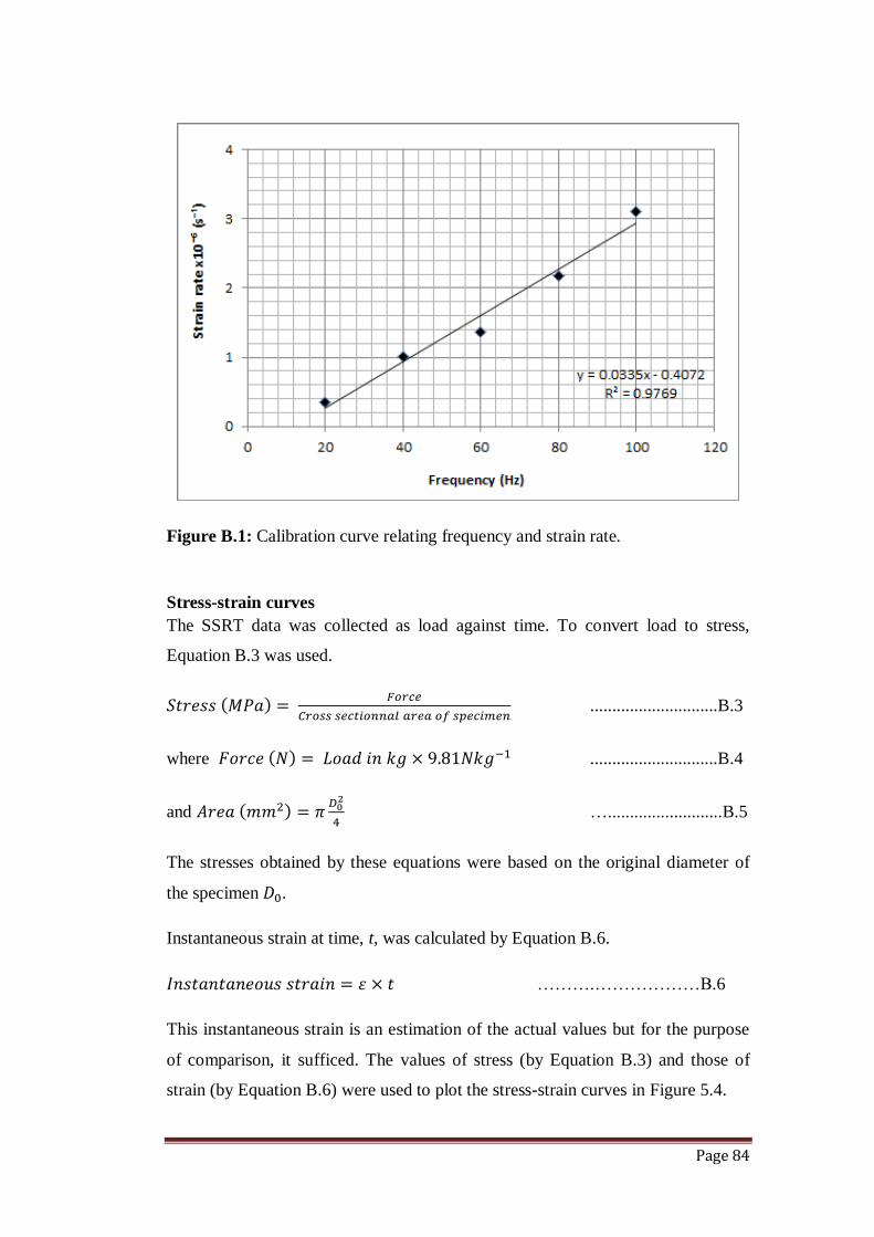
Page 84
Figure B.1: Calibration curve relating frequency and strain rate.
Stress-strain curves
The SSRT data was collected as load against time. To convert load to stress,
Equation B.3 was used.
( )
.............................B.3
where ( ) .............................B.4
and ( )
…..........................B.5
The stresses obtained by these equations were based on the original diameter of
the specimen .
Instantaneous strain at time, t, was calculated by Equation B.6.
……….………………B.6
This instantaneous strain is an estimation of the actual values but for the purpose
of comparison, it sufficed. The values of stress (by Equation B.3) and those of
strain (by Equation B.6) were used to plot the stress-strain curves in Figure 5.4.
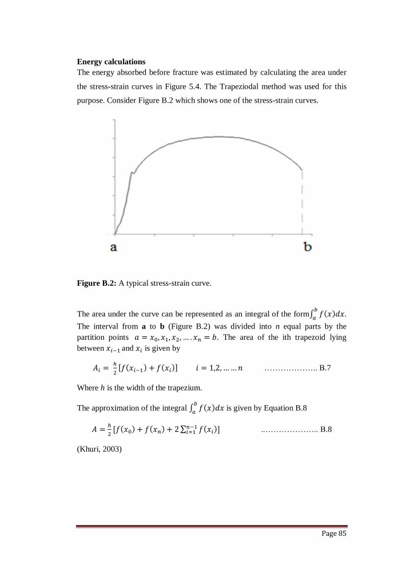
Page 85
Energy calculations
The energy absorbed before fracture was estimated by calculating the area under
the stress-strain curves in Figure 5.4. The Trapeziodal method was used for this
purpose. Consider Figure B.2 which shows one of the stress-strain curves.
Figure B.2: A typical stress-strain curve.
The area under the curve can be represented as an integral of the form∫ ( )
.
The interval from a to b (Figure B.2) was divided into n equal parts by the
partition points . The area of the ith trapezoid lying
between and is given by
[ ( ) ( )] ……………….. B.7
Where h is the width of the trapezium.
The approximation of the integral ∫ ( )
is given by Equation B.8
[ ( ) ( ) ∑ ( )]
..……………….. B.8
(Khuri, 2003)

Page 86
Ductility
Ductility was expressed as percent elongation and area reduction calculated
according to Equations B.9 and B.10.
………………. B.9
………………. B.10