https://doi.org/10.1177/05694345211019714

The American Economist 1 –18

© The Author(s) 2021Article reuse guidelines:

sagepub.com/journals-permissions DOI: 10.1177/05694345211019714

journals.sagepub.com/home/aex

Original Research Article

A Guide to Using the Synthetic Control Method to Quantify the Effects of Shocks, Policies, and Shocking Policies

Bibek Adhikari1

AbstractGovernments introduce various policies intending to improve the overall economy or to influence individual behavior. However, estimating the causal impact of these policies is challenging. I describe how the Synthetic Control Method (SCM) can be used in undergraduate econometrics or capstone courses to estimate the impact of economic policies. The SCM is a data-driven design that provides a systematic way of constructing a comparison group that looks very similar to the group implementing the policy. Thus, it allows us to estimate the policy’s impact by comparing the outcome variable’s post-policy path between the policy group and the comparison group. I review a broad range of policies and events that are analyzed using this method, briefly describe the theory behind the method, discuss various best practices, and provide a step-by-step implementation guide using the adoption of a value-added tax (VAT) by France as an example.JEL Classifications: C01, A1, A2

Keywordssynthetic control method, applied econometrics, policy evaluation

Received: December 7, 2020; Revised: April 12, 2021; Accepted: April 23, 2021

Introduction

Governments at all levels—national, state, and local—introduce policies with an aim to improve the overall economy or to influence the behavior of firms, employees, and citizens. And often, countries and localities around the world experience large-scale disasters ranging from earth-quakes to hurricanes and, most recently, the coronavirus disease 2019 (COVID-19) pandemic. How do these policies and shocks affect the economy and people’s behavior? For instance, how does COVID-19 affect the economy? Which non-pharmaceutical interventions among mask mandate, social distancing, school closure, or lockdown is most effective in reducing the spread

1Illinois State University, Normal, USA

Corresponding Author:Bibek Adhikari, Assistant Professor, Department of Economics, Illinois State University, Stevenson Hall 425, Campus Box 4200, Normal, IL 61790, USA. Email: badhik1@ilstu.edu

1019714 AEXXXX10.1177/05694345211019714The American EconomistAdhikariresearch-article2021

2 The American Economist 00(0)

of COVID-19? How do gun policies, such as right-to-carry (RTC) concealed handgun laws and Stand Your Ground laws that have been introduced in many states, affect gun violence and homi-cide? What are the economic consequences of a global surge of populism such as Brexit or the election of Donald Trump as the president of the United States? These are important and some-times controversial policies with the potential to affect the lives and welfare of millions of peo-ple. Importantly, these are a small sample of some of the great questions you can study in an econometrics class or a capstone experience.

However, assessing the actual causal effects of these policies is challenging because once a unit (e.g., individuals, firms, or states) implements such policy, it is impossible to factually know what would have happened to that unit had it not implemented the policy. If we can somehow find another unit that did not implement the policy but is otherwise very similar to the unit imple-menting the policy (i.e., a twin or a doppelganger), then we can compare the behavior of the unit implementing the policy (also called the treated unit) and its doppelganger (or, the comparison unit) to infer the impact of the policy (Born et al., 2019b). Of course, the challenge is that such doppelgangers rarely exist as no two individuals, counties, states, countries are very similar to each other.

In this article, I describe a new econometric technique called Synthetic Control Method (SCM) that can be used to construct the synthetic unit—a doppelganger that did not implement the pol-icy but was behaving in a very similar way to the treated unit for a long period of time (Abadie & Gardeazabal, 2003; Abadie et al., 2010, 2015). More formally, the SCM is a data-driven research design that provides a systematic way of constructing a synthetic unit from the weighted average of units from the comparison units, such that the constructed synthetic unit matches the path of the outcome variable as well as all the important predictors of the outcome variable for many periods before the policy’s implementation. Once such synthetic unit is constructed, we can simply take the difference between the outcome of the treated unit and that of the synthetic unit to find the causal impact of treatment. The idea being that if the treated unit and the synthetic unit were on a very similar path for many periods before the treatment and then their path starts diverging right after the implementation of the treatment, then we can attribute the divergence in the path to the treatment.

The SCM can be applied to answer numerous questions of interest and I believe it is very suit-able for undergraduate research projects. Its suitability for undergraduate research comes from three things. First, Abadie et al. (2010) have made the synth package that enables one to use the method freely available in all the major statistical software such as Stata and R.1

Second, SCM does not require micro-data or big data that are usually hard to access and require significant time investment before they can be used for analysis. The SCM is best suited for aggregate data at the city, state, or country level that are easily available from public sources such as the World Bank, International Monetary Fund, or the Federal Reserve Economic Data (FRED) website.

Third, the SCM allows estimating the causal effect of a policy intervention in settings where only a few treated and control units are observed over a long time period. Thus, some of the most important policies, such as the ones mentioned above or the ones I review in the next sec-tion, can be analyzed using the SCM and publicly available data. For instance, many states and cities have legalized medical and recreational marijuana use, decriminalized drug use, passed right-to-work laws, paid family and medical leave, increased minimum wage, and so on that can be analyzed using this method. Most of these policy changes are frequently reported in newspa-pers and magazines. There also exists an excellent database of various policy changes in the U.S. states since 1900 (Jordan & Grossmann, 2020). Students can also analyze the impact of the policies reviewed in this article but on different outcomes of interest. Any of these approaches would guide students through the analysis part but still allow for significant original research experience.

Adhikari 3

In the next section, I review various studies that use the SCM to estimate the causal impact of shocks like natural and human-caused disasters, unique events like the presidency of Hugo Chavez and Brexit, common policies like tax reforms, carbon taxes, and gun laws, and “shocking policies” like decriminalization of drug use and prostitution. I will then explain the fundamental challenge of causal inference and describe how SCM can be used to overcome such challenges and estimate the causal impact of the treatment. Next, I will provide various best practices and a step-by-step guide using the adoption of a value-added tax (VAT) by France as an example. The next section concludes the article.

Review of the Literature Using the SCM

Regional integration, disintegration, and populism

Numerous studies use the SCM to study the economic effects of regional integration, disintegra-tion, and populism. In fact, Abadie et al. (2015), who expanded the SCM, illustrated the method’s main ideas by estimating the economic impact of the 1990 German reunification on West Germany. They find that reunification reduced gross domestic product (GDP) per capita of West Germany by about US$1,600 per year on average over the 1990–2003 period compared with Synthetic Germany, which comprised Austria, Japan, Netherlands, Switzerland, and the United States. In the U.S. context, Hall et al. (2020) also find no effect or negative effect of city–county consolidations on per capita income, population, and employment. On top of that, they find that consolidation can deepen the urban-rural divide by accelerating the decline of rural populations relative to those of urban areas.

Many studies quantify the economic effects of joining, abstaining, or exiting from the European Union (EU) or adopting the Euro as their national currency using the SCM. For instance, Campos et al. (2019) study the impact of joining the EU from 1973 to 2004. They find a large and positive (about 10% on average) growth effect of joining the EU in all countries except for Greece. Campos et al. (2015) study the peculiar case of Norway that, despite qualify-ing for full EU membership, decided only to join the European Economic Area that gave Norway access to the Single Market but avoided full institutional integration. They find that had Norway chosen full integration, the average Norwegian region would have experienced an annual pro-ductivity growth increase of about half a percentage point. Saia (2017) studies the impact of the adoption of the Euro as the national currency and finds that it led to an increase in intra-European trade flows by about 19% to 55%. He also estimates that the trade flows would have been 16% higher between the United Kingdom and its main trading partners if the United Kingdom had joined the Euro. However, the effect of adopting the Euro on GDP per capita was mixed. Puzzello and Gomis-Porqueras (2018) find that adopting the Euro had a negative impact on the GDP per capita of Belgium, France, Germany, and Italy, no significant change in the Netherlands, and a positive and significant impact on GDP per capita of Ireland. Finally, two articles estimate the impact of the United Kingdom’s decision to leave the EU (i.e., Brexit). Born et al. (2019b) find that the Brexit vote resulted in a cumulative loss of £55 billion in the United Kingdom’s GDP by the end of 2018. Breinlich et al. (2020) find that U.K. firms increased investment to the remain-ing EU states by 17%, whereas the investment from these EU states to the United Kingdom decreased by about 9%. They conclude that United Kingdom being a smaller economy than the EU caused this disparate impact as U.K. firms increased investment to set up subsidiaries in the EU countries to retain access to the EU market after Brexit, whereas the firms from EU members did not reciprocate.

There has been a rapid increase in nationalism or populism across the world, with more than 16 countries being governed by populist governments in 2018 (Funke et al., 2020). Born et al. (2019a) study the impact of Trump’s presidency on the U.S. economy. They did not find any

4 The American Economist 00(0)

positive impact on GDP per capita, employment, labor force participation, or unemployment rate in the United States under Trump’s administration compared with the synthetic United States. Grier and Maynard (2016) study the impact of Hugo Chavez on the Venezuelan economy and find that Chavez’s administration had a significant negative impact on GDP per capita and no improvements on poverty, health, or inequality. In a related study, Absher et al. (2020) estimate the impact of populist leaders in Venezuela, Nicaragua, Bolivia, and Ecuador and find that GDP per capita in these countries decreased by about 20% compared with their corresponding Synthetic units while there was no significant improvement in the inequality or health outcomes. Finally, similarly negative effects on income per capita are found in a comprehensive study of 50 populist presidents and prime ministers between 1900 and 2018 (Funke et al., 2020).

Deregulation, liberalization, and structural reforms

How do structural reforms of the economy such as deregulation of the labor market, product market, or trade liberalization affect the economy? Adhikari et al. (2018) study six of the most extensive structural reforms in the advanced economy of New Zealand, Australia, Denmark, Ireland, Netherlands, and Germany. They find a positive impact on four of the countries, but no impact on the other two countries, with suggestive evidence that reforms implemented under weak macroeconomic conditions did not improve economic growth. Nannicini and Billmeier (2011) and Billmeier and Nannicini (2013) study the impact of trade liberalization in transition-ing economies as well as in a worldwide sample of countries. They find that liberalizing the economy had a positive effect in most regions, except in Africa, which had no significant impact. Eren and Ozbeklik (2016) study the impact of Oklahoma’s right-to-work law that prohibited union security agreements between companies and unions, meaning that employees in unionized firms cannot be required to join the union or pay the union dues although they may still receive the benefits that paying members receive. They find that such laws decreased private-sector unionization rates but did not affect the total employment rate, average wages in the private sec-tor, or average wage in the manufacturing sector.

Flat tax, sin tax, and tax reforms

Taxes are a fact of life. So much so that, after the U.S. constitution was written, Benjamin Franklin wrote to Jean-Baptiste Le Roy, “Our new Constitution is now established, and has an appearance that promises permanency; but in this world nothing can be said to be certain, except death and taxes.” Government taxes our income, consumption, and wealth to raise revenue, but it also imposes a “sin tax” on goods with negative externality such as cigarettes, alcohol, marijuana, and carbon emission. What are the intended and unintended consequences of such taxes? Several studies try to answer these questions using the SCM.

Do major tax reforms affect economic growth and inequality? Adhikari and Alm (2013, 2016) study the impact of replacing the progressive income tax with a flat-rate income tax by eight Eastern European countries and find a positive and statistically significant impact in seven out of eight countries. Rubolino and Waldenström (2020) study the impact of flattening the income tax rate on top income shares in Australia, New Zealand, and Norway using the SCM. They find that these reforms increased the income shares of the top percentile of the income distribution. Adhikari (2020) estimates the impact of replacing sales tax with a VAT on GDP per worker, total factor productivity, and capital deepening in a sample of 33 countries that implemented such reforms compared with their respective synthetic controls. He finds that VAT had a positive and significant impact but only on developed countries.

Do individuals move to different countries to avoid high taxes? Kleven et al. (2013) study the effect of top tax rates on the international mobility of football players and Akcigit et al. (2016)

Adhikari 5

study the international mobility of “superstar” inventors. Both studies find that a sizable number of “superstar” taxpayers move to a different country to avoid higher top marginal tax rates.

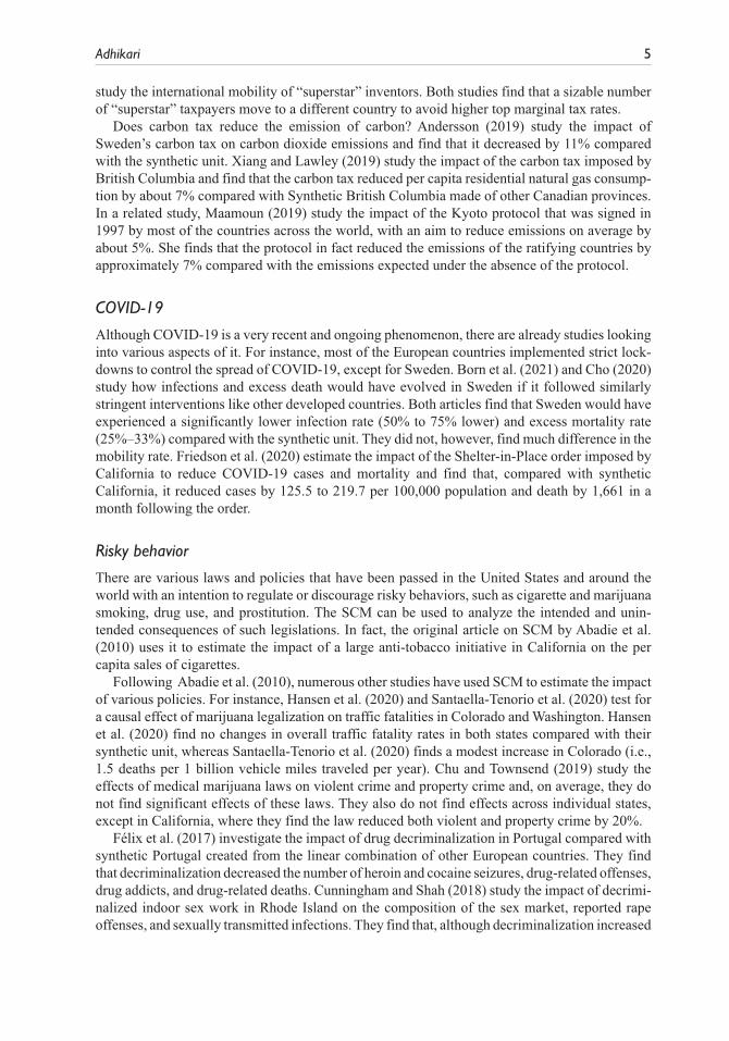
Does carbon tax reduce the emission of carbon? Andersson (2019) study the impact of Sweden’s carbon tax on carbon dioxide emissions and find that it decreased by 11% compared with the synthetic unit. Xiang and Lawley (2019) study the impact of the carbon tax imposed by British Columbia and find that the carbon tax reduced per capita residential natural gas consump-tion by about 7% compared with Synthetic British Columbia made of other Canadian provinces. In a related study, Maamoun (2019) study the impact of the Kyoto protocol that was signed in 1997 by most of the countries across the world, with an aim to reduce emissions on average by about 5%. She finds that the protocol in fact reduced the emissions of the ratifying countries by approximately 7% compared with the emissions expected under the absence of the protocol.

COVID-19

Although COVID-19 is a very recent and ongoing phenomenon, there are already studies looking into various aspects of it. For instance, most of the European countries implemented strict lock-downs to control the spread of COVID-19, except for Sweden. Born et al. (2021) and Cho (2020) study how infections and excess death would have evolved in Sweden if it followed similarly stringent interventions like other developed countries. Both articles find that Sweden would have experienced a significantly lower infection rate (50% to 75% lower) and excess mortality rate (25%–33%) compared with the synthetic unit. They did not, however, find much difference in the mobility rate. Friedson et al. (2020) estimate the impact of the Shelter-in-Place order imposed by California to reduce COVID-19 cases and mortality and find that, compared with synthetic California, it reduced cases by 125.5 to 219.7 per 100,000 population and death by 1,661 in a month following the order.

Risky behavior

There are various laws and policies that have been passed in the United States and around the world with an intention to regulate or discourage risky behaviors, such as cigarette and marijuana smoking, drug use, and prostitution. The SCM can be used to analyze the intended and unin-tended consequences of such legislations. In fact, the original article on SCM by Abadie et al. (2010) uses it to estimate the impact of a large anti-tobacco initiative in California on the per capita sales of cigarettes.

Following Abadie et al. (2010), numerous other studies have used SCM to estimate the impact of various policies. For instance, Hansen et al. (2020) and Santaella-Tenorio et al. (2020) test for a causal effect of marijuana legalization on traffic fatalities in Colorado and Washington. Hansen et al. (2020) find no changes in overall traffic fatality rates in both states compared with their synthetic unit, whereas Santaella-Tenorio et al. (2020) finds a modest increase in Colorado (i.e., 1.5 deaths per 1 billion vehicle miles traveled per year). Chu and Townsend (2019) study the effects of medical marijuana laws on violent crime and property crime and, on average, they do not find significant effects of these laws. They also do not find effects across individual states, except in California, where they find the law reduced both violent and property crime by 20%.

Félix et al. (2017) investigate the impact of drug decriminalization in Portugal compared with synthetic Portugal created from the linear combination of other European countries. They find that decriminalization decreased the number of heroin and cocaine seizures, drug-related offenses, drug addicts, and drug-related deaths. Cunningham and Shah (2018) study the impact of decrimi-nalized indoor sex work in Rhode Island on the composition of the sex market, reported rape offenses, and sexually transmitted infections. They find that, although decriminalization increased

6 The American Economist 00(0)

the indoor sex market’s size, it decreased reported rape offenses by 30% and female gonorrhea incidence by about 40%.

Guns and crimes

Gun violence and other violent crimes are major public safety issues in the United States and many states have passed laws with an aim to reduce them. However, such laws are controversial and thus it is important to know the effects of such policies. Donohue et al. (2019) study the impact of RTC concealed handgun laws on violent crime and find that RTC laws are associated with 13% to 15% higher violent crime rates compared with their synthetic counterpart. Guettabi and Munasib (2020) study the impact of Stand Your Ground laws—a modification of the “no duty to retreat” law outside of one’s residence on firearm deaths that has been adopted in more than 20 U.S. states following Florida’s adoption in 2005. They find that death from guns would have been substantially lower in Alabama, Florida, and Michigan had these states not passed Stand Your Ground laws. However, they did not significantly impact the rest of the 19 states that passed Stand Your Ground laws.

Pinotti (2015) studies the impact of organized crime in two regions of southern Italy exposed to mafia activity and finds that the mafia’s presence lowers GDP per capita by 16% in these regions compared with similar regions in other parts of Italy.

Immigration

How does immigration affect the wages and employment of native workers? One of the classic studies on this topic is Card (1990), who studied the impact of almost 125,000 Cuban refugees’ arrival in Miami in what is known as the Mariel Boatlift. He found that its impact on the employ-ment and wages of low-skilled non-Cubans in Miami was economically insignificant. Peri and Yasenov (2019) reexamined the labor market effect of the Mariel Boatlift using the SCM. They also did not find any significant difference in the wages of workers in Miami relative to synthetic Miami. However, Dustmann et al. (2017) find that a unique immigration policy in Germany that allowed neighboring Czech workers to seek employment in German municipalities along the border but denied residence rights led to a modest decline in average local wages and a sharp decline in local employment of natives compared with their respective synthetic controls.

Many fear that large-scale immigration can negatively affect the institutions and social norms of countries that are at the receiving end of the migration. Are these fears grounded in actual evidence? Powell et al. (2017) study this question in the context of Israel, leveraging the large immigration inflow from the Soviet Union in the 1990s. They find that mass migration from a country with very different political and economic institutions can impact institutions in a desti-nation country and find that Israel enjoyed greater economic freedom and moved further away from socialism compared with synthetic Israel, mostly due to the immigrant’s influence on the political process.

Disasters and terrorism

Cavallo et al. (2013) study the impact of catastrophic natural disasters on economic growth and find that only extremely large disasters have a negative effect on output in both the short and the long runs. They find that even extremely large disasters do not display any significant effect on economic growth if it is not followed by political upheaval.

Grossman and Slusky (2019) study the impact of large exposure to lead and other contami-nants caused when the city of Flint in Michigan switched its public water source from Lake Huron to Flint River. They compare the change in the fertility rate and health at birth in Flint

Adhikari 7

before and after the water switch to the changes in similar cities. They find that Flint’s fertility rates decreased by 12% and decreased overall health at birth.

The Fundamental Challenge of Causal Inference and the SCM

Fundamental challenge of causal inference

The fundamental challenge of estimating the causal impact of a policy is that it is only possible to observe what happened after the policy was introduced. Once the policy is in place, it is impos-sible to factually know what would have happened without that policy in place. That is, we can observe the number of COVID-19 cases in a city with intervention, but it is not possible to observe how many cases the city would have had in this time period had they not put such restric-tions in place. This hypothetical situation of what would have happened in the absence of the intervention is called the “counterfactual” and, unfortunately, the counterfactual will always be unknown. The best we can do is credibly estimate the missing counterfactual. Once we estimate the missing counterfactual, we can estimate the causal impact of treatment by comparing the dif-ference in outcomes between the treated group and its counterfactual.

One of the best ways of finding whether and how a treatment (i.e., shock or policy in our case) affects a particular outcome is by conducting a randomized experiment. This usually entails ran-domly drawing some units (e.g., individuals, firms, or states) and placing them into two groups called the “treatment group” and the “control group.” The treatment group receives treatment and the control group does not, which is basically an attempt to fulfill the ceteris paribus assumption by only changing one thing between the treatment group and the control group: exposure to treat-ment. Thereafter, to find the causal impact of treatment, one simply takes the difference between the outcome of the treated group and that of the control group.

Randomized experiments are very popular in natural sciences and it has become quite popular in economics too. In fact, Kahneman and Smith won the 2002 Nobel prize in economics for establishing laboratory experiments as a tool in economic analysis and Banerjee, Duflo, and Kremer won the 2019 Nobel prize for pioneering the use of randomized controlled trials to study poverty.

However, experiments, especially randomized controlled trials, are relatively rare in econom-ics because they are often very costly to conduct, politically controversial, and face various ethi-cal issues. For example, it would be unethical to randomly restrict some citizens from wearing masks to study the causal effect of masks on the spread of COVID-19. It would be very expen-sive to test the impact of Universal Basic Income on long-term life satisfaction by giving some citizens a monthly income solely for experimentation. And it would be politically infeasible to study the effects of gun laws by randomly assigning gun policies to some states. Thus, a large share of the empirical work in economics relies on policies that are not determined randomly but actively chosen.

As policies that are not determined randomly usually do not generate data with random assign-ment to the policies, it will be difficult to estimate the causal impacts of such policies. Let me explain this challenge using COVID-19 as an example. Did the non-pharmaceutical interventions reduce the spread of the COVID-19 virus? To answer this question, one could compare the spread of COVID-19 in cities that introduced non-pharmaceutical interventions with the spread in cities without such interventions. A cursory observation (or even a cross-sectional regression) will likely show that cities with the most stringent restrictions are the ones that also experience the greatest spread of COVID-19. Does it mean that these restrictions cause an increase in COVID-19 cases? It is most likely that the causation is reversed in this case. The cities with higher COVID-19 cases choose more stringent restrictions than cities with a lower number of cases. One could also com-pare the number of COVID-19 cases before and after the intervention in the city that introduced

8 The American Economist 00(0)

intervention. However, given that these cases are increasing over time, often exponentially, a simple before-after comparison (or a time series regression) will likely show that COVID-19 increased after the intervention. These factors, which may be unknown to the researchers, can induce a correlation between non-pharmaceutical intervention policies and COVID-19 cases that do not indicate what would happen if the interventions were not introduced.

Fortunately, recent improvements in applied econometric techniques allow us to estimate the causal impact of these types of interventions by leveraging natural experiments or quasi-experi-ments. These quasi-experiments are basically “quasi-random” assignment of treatment to some groups due to natural events, various policies, rules, and regulations passed at some jurisdictions but not others, arbitrary age threshold above which you can purchase alcohol and tobacco products, and so on. Some of the most popular techniques in applied economics are difference-in-differences, instrumental variable, regression discontinuity design, and SCM. Whereas traditional econometrics textbooks do not cover these methods, a few textbooks have started covering the first four methods (e.g., see Angrist & Pischke 2009, 2015). However, the SCM has not yet been covered in a textbook except for Cunningham (2021).2 Thus, in this article, I attempt to close that gap.

SCM

Suppose we have J + 1 units (i.e., city, state, or country), where Unit 1 introduces the policy we are interested in evaluating at time T0 +1. Let’s call Unit 1 the treated unit as it introduced the policy and the remaining J units that did not introduce the policy the donor pool from which synthetic unit will be constructed. Let T0 be the number of pre-policy periods (i.e., months, quar-ters, or years), with 1 ≤ T0 < T. Also, let Yit

NP be the outcome variable observed for unit i at time t with no policy (NP), and Yit

P be the outcome variable observed for unit i at time t with policy (P). The observed outcome variable can be written as

YY intheabsenceof policy

Y Y D inthe presencit

itNP

itP

itNP

it it

=≡ + τ eeof policy

,

where τit itP

itNPY Y= −( ) is the effect of the policy for unit i at time t and Dit =1 if t T> 0 and

i =1, and Dit = 0 otherwise.For any treated unit, we can only observe Yit

P in the post-policy period. However, to estimate the treatment effect, we need to estimate the counterfactual Yit

NP, which is the outcome variable of the unit that introduced the policy had the unit not introduced it. To estimate the counterfac-tual, we use the linear factor model of the form

Y ZitNP

t t i t i it=∝ + + +θ λ µ ε

where ∝t is an unknown common factor with constant factor loadings across units, Zi is a vector of observed covariates with coefficients θt , µi is a ( )F ×1 vector of unknown parameters, λt is a ( )1×F vector of unobserved common factors, and εit are idiosyncratic error terms with zero mean.

Let us define a synthetic control unit as a weighted average of the units in the donor pool. That is, a synthetic control can be represented by a J × 1 vector of weights, W = (w2, . . ., wJ+1)' such that wj ≥ 0 for j = 2, . . ., J + 1 and w2+ . . . + wJ+1= 1, where vector W represents a potential synthetic control. Then the outcome variable for each potential synthetic control unit is given by

j

J

j jt t t

j

J

j j t

j

J

j i

j

J

j jtw Y w Z w w=

+

=

+

=

+

=

+

∑ ∑ ∑ ∑= + + +2

1

2

1

2

1

2

1

α θ λ µ ε .

Adhikari 9

Now let us suppose that there are ( ,..., )* *w wJ2 1+ ' , such that the following condition holds.

j

J

j j

j

J

j jT T

j

J

j jw Y Y w Y Y w Z Z=

+

=

+

=∑ ∑ ∑= … = =2

1

1 11

2

1

1

2

10 0

* * *, , , .

Thus, the treatment effect at time t ϵ {T0+1, . . ., T} can be estimated by

τ1 1

2

1

t t

j

J

j jtY w Y= −=

+

∑ * .

To find the optimal weights, let the ( )T0 1× vector K = ( ,..., )k kT1 0' define a linear combina-

tion of pre-policy outcomes, Y k YjK

s

T

s js==∑1

0

, where j belongs to { ,..., },1 1J + j=1 denotes

treated unit and j ≠ 1denote donor units. Consider M of such linear combinations defined by the vectors ( ,..., )K KM1 . Let X1 be ( Z Y YK KM

1 1 11' ', ,..., ) , the vector of pretreatment variables

that we aim to match as closely as possible for the treated unit. Let X0 be the matrix where each column of the matrix is a vector of the same pretreatment variables for each potential donor unit. The synthetic control algorithm chooses W * to minimize the distance X1 0−X WV X W V X W= − −( ) ( )1 0 1 0X X‘ , where V is a symmetric, positive semi-definite and diagonal matrix, such that the root mean square prediction error (RMSPE) of the outcome variable is mini-mized for the pre-policy periods, which ensures that larger weights is given to those variables that have the highest predictive power.

How to assess the pretreatment fit of the synthetic unit?

To assess whether the comparison unit created using SCM is a good counterfactual, we need to measure how well it resembles the treated unit before the treatment. Abadie et al. (2010) use RMSPE of the outcome variable to measure fit or lack of fit between the path of the outcome variable for treated unit and its synthetic counterpart, defined as

RMSPET

Y w Yt

T

t

j

J

j jt= −

= =

+

∑ ∑1

0 1

1

2

12

0

* .

When the RMSPE is 0, it means that the synthetic unit perfectly matched the pre-policy trajec-tory of our treated unit, indicating a perfect fit. However, when the RMSPE is not 0, it becomes difficult to map the magnitude of RMSPE to the synthetic unit’s goodness of fit. Adhikari and Alm (2016) developed a “pretreatment fit index” that allows one to assess the quality of the pre-treatment fit easily. To do so, they first calculate benchmark RMSPE, which is defined as

Benchmark RMSPET

Yt

T

t= ( )=∑1

0 1

12

0

.

Thereafter, the pretreatment fit index is defined as the ratio of the RMSPE and the benchmark RMSPE:

Fit IndexRMSPE

benchmark RMSPE= .

10 The American Economist 00(0)

A fit index of X means that the RMSPE is equivalent to the RMSPE obtained when the differ-ence between the treated and the synthetic unit is X percent on each pretreatment year. If the RMSPE is 0, then the fit index will be 0, indicating a perfect fit. If the RMSPE is equal to the benchmark RMSPE, then the fit index will be 1, indicating that the fit is similar to that created by a synthetic unit that is twice as big (or half as small) as the treated unit. The fit index can even be greater than 1 in cases where the outcome variable of the treated unit is bigger by a magnitude of two or more (or smaller by a magnitude of half or less). A fit index greater than 1 usually indi-cates a poor fit and such synthetic unit should not be used as the counterfactual, especially when the outcome variable is say, GDP per capita, where it is safe to assume that a synthetic unit with twice the GDP per capita of the treated unit cannot reasonably be a good counterfactual. When the outcome variable is, say, inflation rate, then the fit index of 1 could mean that the treated unit has inflation of 2% while the control unit has inflation of 4%. In such a case, one might still be able to use the counterfactual with the fit index of 1 or more, but one must be very cautious and properly justify the use.

How to assess whether the estimated effects are statistically significant?

The SCM is usually used when the treatment effect arises from the change in policy by a small group of units and where data are usually of small sample size. Thus, the standard large-sample significant tests that are typically used for inference, such as calculating standard error, confi-dence intervals, or p values, are not appropriate. Instead, we can conduct placebo experiments and calculate pseudo p values to test whether the estimated impact of the policy of interest could be driven entirely by chance. Specifically, we can conduct a series of placebo experiments by iteratively estimating the “placebo” treatment effect for each unit in the donor pool (i.e., untreated units) by falsely assuming that these units introduced our policy of interest in the same year the actual treated unit did. Thereafter, we can run the SCM analysis to find the placebos treatment effect for these placebo units. This iterative procedure provides a distribution of estimated pla-cebo treatment effects for the units with no policy. If the placebo experiments create enough placebo treatment effects of magnitude greater than the one estimated for the treated unit, then we conclude that there is no statistically significant evidence of an effect of policy in the treated unit. If the placebo experiments create placebo treatment effects of magnitude greater than the one estimated for the treated unit in more than 10% of the placebo experiments (i.e., if the cor-responding pseudo p value is greater than .1), then we can conclude that there is no statistically significant evidence of an effect of the policy in the treated unit. If the corresponding pseudo p value is less than .1, then we can conclude that there the policy had a statistically significant impact on the treated unit.

Diagnostics using leave-one-out (LOO) test

We can implement a LOO test to check the sensitivity of our baseline estimates to the inclusion of specific donor countries in the synthetic unit’s construction. To apply this test, you iteratively reestimate the baseline model, excluding in each iteration one of the donor countries that received positive weights in the baseline model. If the LOO synthetic units closely track the baseline syn-thetic units in all iterations, then the estimated treatment effects will be similar no matter which donor country is removed from the sample, ensuring that the results are not driven by shocks experienced by some individual donor country, thus increasing our confidence that the estimated impact is the true impact of the policy in question.

Adhikari 11

Best Practices and an Illustrated Example

Best practices

The first step in running SCM is to identify the introduction or removal of a policy you are inter-ested in. The impact of small interventions is difficult to detect using this method; thus, the policy of interest should have the potential to affect the outcome of interest significantly.

The second step is to identify the potential donor units that did not make such policy changes. It is important to carefully choose the potential donor units because you want poten-tial donor units to be similar to the treated unit. Thus, you might want to limit the potential donor pool to the countries from the same geographic region, or same income group (i.e., developing countries or developed countries), or similar demographic, and so on depending on your research question. However, limiting the potential donor unit this way has a tradeoff too. If there are not enough countries in the donor pool, the SCM might not be able to find a syn-thetic unit with a good pretreatment fit. Even if it finds a synthetic unit with a good pretreat-ment fit, there might not be enough countries in the donor pool for running placebo analysis, which means that the size and the power of the inference will be small and unreliable. There are a couple of different ways to tackle this. For instance, Billmeier and Nannicini (2013) run the SCM twice, one restricting the donor pool to the country from the same geographic region and the other without that restriction. Adhikari and Alm (2016) use the “hybrid donor pool,” where the donor pool for each treated country is restricted to the same geographic region. However, they run the placebo experiment using a worldwide sample of countries, but placebo treatment effects are calculated by restricting the donor pool of each placebo unit to their respective region. That is, they calculate regional placebo treatment effects for the global pool of countries.3

Third, you need to obtain the data you want to evaluate and prepare the data for analysis. You need a panel data set and it must be declared as a panel data set in Stata, which can be done using tsset command. You need to choose how many years of pretreatment data you want to use for constructing the synthetic control unit and how many years of posttreatment data you want to use to evaluate the impact of the treatment. It is better to have many pretreatment periods because the longer treated units and synthetic units are moving along the same path, the more likely it is that they would move along the same path in the absence of the treatment. However, it is best to have about 5 to 10 periods of posttreatment data because the further away we go from the treatment date, the more likely it is that other shocks or policies are implemented, which can contaminate our treatment effect.

Fourth, outcome variables that are very volatile or include random noise, like stock market returns, are usually not suitable for analysis using SCM. Thus, you will notice most analyses using the SCM use variables, such as GDP per capita, COVID cases per capita, crimes per capita, and so on.

Fifth, there should not be any missing observation for the outcome variable in the full sample period—for both the treatment unit and donor units. If there are just a few missing values, then you can interpolate the missing values. If there are lots of missing values, then the data might not be suitable for analysis.

Sixth, there should be at least one non-missing observation of all the predictor variables in the pretreatment period for both the treatment unit and all donor units. This is because we usually use the average value of predictors in the pretreatment years. However, if we have more non-missing observations in the pretreatment years, then we will have more confidence that the averages cal-culated reflect the true average due to the law of large numbers. Thus, having full and balanced panel data for predictors is ideal but not necessary.

Seventh, if there are some outliers in the data, they should be removed as the SCM matches in the pretreatment period and if it matches on the outlier, then that match might not reflect the true path of the outcome variable.

12 The American Economist 00(0)

Once you prepare the data, you are ready to run the SCM module. To do so, you can type the following in Stata: synth Y_var Y_var X_var, trunit (treated unit) trperiod (treatment period) keep (filename) nested fig replace, where the first instance of Y_var denotes the outcome vari-able, the second instance of Y_var denotes the use of the outcome variable as the predictor vari-able, and the X_var represents the list of all other predictor variables.

The synth module by default uses the averages of all predictor variables over the entire pre-intervention period, ignoring missing values when taking the averages. Thus, having some miss-ing values in the predictors is fine. I also recommend using the averages of predictor variables and including the outcome variable’s average as one of the predictors. I do not advise using all pretreatment observations of the outcome variable as separate predictors as doing so makes all other covariates irrelevant even when these covariates are important predictors of the outcome variable (Kaul et al., 2015).

You need to put the unit id for the treatment unit in trunit (. . .) and the treatment year in the trperiod (. . .). The nested option instructs the program to search for the best fitting convex com-bination of the control units that achieve even lower RMSPE than the default option although it might increase the run time of the program by a little. The fig option produces the figure showing the trajectory of the outcome variable of the treated unit and control unit for the full sample period. However, the figure for placebo treatment effects and other diagnostic tests needs to be created manually. Finally, the keep (. . .) option saves a data set with the results that can be used to process the result further. Now, let us put this theory and best practices to test.

Illustrative example

In this section, I will use the adoption of VAT by France in 1968, one of the first countries in the world to do so, as the treatment to illustrate the use of the SCM.4 My aim is to both illustrate how the method can be implemented in Stata and to provide a guide on how to describe the pretreat-ment fit, treatment effect, inference, and robustness tests. Thus, for each of these, I will start with an implementation guide and end with a guide to discuss the output.

I want 10 pretreatment years and 5 posttreatment years; thus, the sample period will be 1958 to 1973. I drop any countries that adopted a VAT in the sample period as I am interested in esti-mating the impact of adopting a VAT. I also drop various other countries that either experienced major shock in their economy or are prone to have large shocks. More precisely, I drop countries flagged as an outlier by the Penn World Table database, small island countries, countries from the Soviet Union, countries with oil and gas as the main source of income, and countries that engaged in a major war during the sample period. This leaves me with 30 countries in the donor pool.

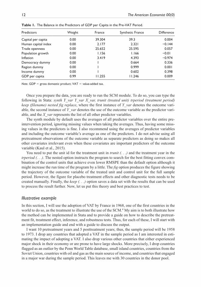
Table 1. The Balance in the Predictors of GDP per Capita in the Pre-VAT Period.

Predictors Weight France Synthetic France Difference

Capital per capita 0.00 39.304 39.3 0.004Human capital index 0.00 2.177 2.321 −0.144Trade openness 0.00 25.652 25.595 0.057Population growth 0.00 1.156 1.166 −0.01Inflation 0.00 3.419 4.393 −0.974Democracy dummy 0.00 1 0.664 0.336Region dummy 0.00 1 0.999 0.001Income dummy 0.00 1 0.602 0.398GDP per capita 0.99 11.255 11.246 0.009

Note. GDP = gross domestic product; VAT = value-added tax.

Adhikari 13

In the first step, the SCM algorithm assigns weights to each of the covariates that can range from 0% to 100% but must add up to 100%, such that the variables that can most accurately predict the trend in the outcome variable of France before the treatment receive the highest weights. Table 1 presents the weight assigned to each predictor. The most predictive covariate, in this case, was the pretreatment average of GDP per capita, which accounted for 99% of the weight. The other variables I included, capital per capita, human capital index, trade openness, population growth rate, inflation rate, and three dummy variables that have value 1 if they are a democracy, belong to the same geographic region as France, and belong to the same income group as France, made up for the remaining 1%.

Next, the algorithm finds synthetic France as a linear combination of countries in the donor pool, such that synthetic France matches the values of the variables with the highest predictive power as closely as possible and the RMSPE of the outcome variable is minimized. The differ-ences in the pretreatment average of covariates between France and synthetic France are pre-sented in Table 1 and the differences are minor for all predictors. The RMSPE is 0.1167 (or a 0.01 fit index). Thus, both the predictors and the RMSPE of the outcome variable show excellent pretreatment fit between France and synthetic France.

The individual countries in the synthetic unit and their contribution (which ranges from 0% to 100% and adds up to 100%) are as follows: Spain (32.8%), Finland (23.4%), Canada (19.3%), United States (16.9%), Greece (6.9%), and Switzerland (0.6%). The remaining countries in the donor pool are assigned a 0% weight by the algorithm. Put differently, the weights reported above indicate that GDP per capita trends in France prior to the adoption of a VAT is best repro-duced by a combination of Spain, Finland, Canada, the United States, Greece, and Switzerland.

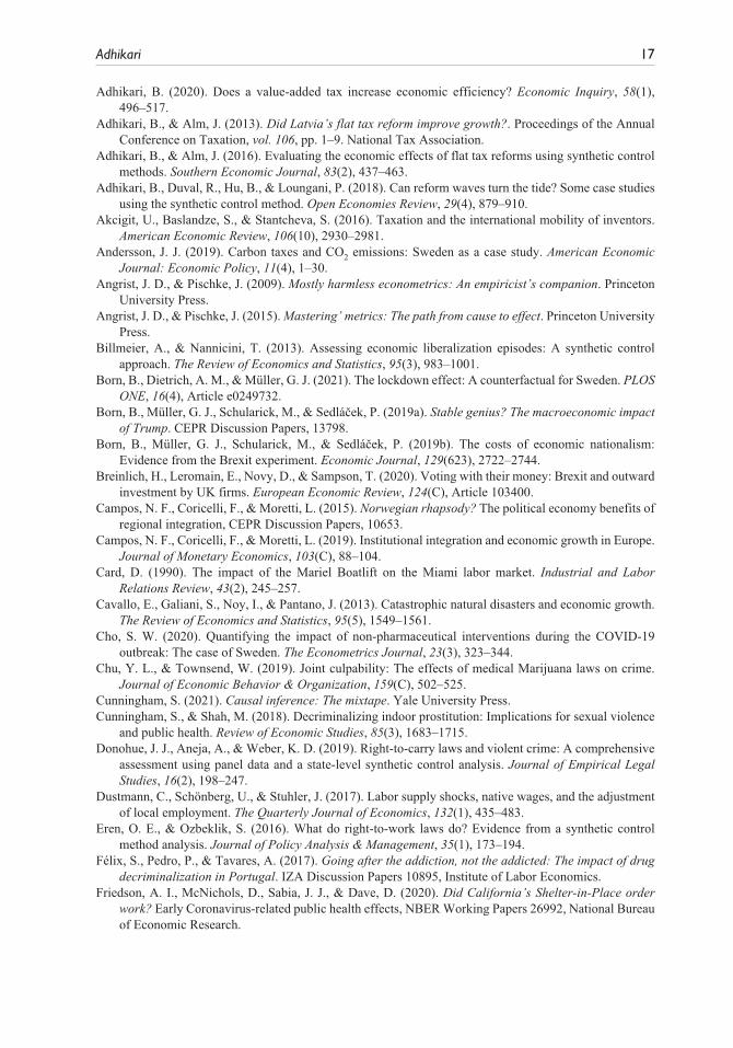
Figure 1. The impact of VAT on GDP per capita of France versus synthetic France.Note. VAT = value-added tax; GDP = gross domestic product.

14 The American Economist 00(0)

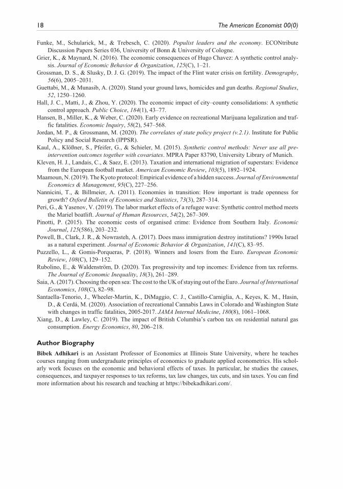
Figure 2. The true impact of VAT on GDP per capita in France versus various Placebo impacts.Note. VAT = value-added tax; GDP = gross domestic product.

Figure 3. The leave-one-out (LOO) distribution of the synthetic units for France.Note. GDP = gross domestic product.

Adhikari 15

Results

The impact of VAT on the GDP per capita of France is illustrated in Figure 1. The vertical dashed line indicates the treatment year. The difference between the connected line (GDP per capita of France) and the dashed line (GDP per capita of synthetic France) before the treatment year indi-cates the quality of pretreatment fit. The same difference after the treatment year indicates dynamic treatment effects. We see a modestly positive impact of VAT on GDP per capita. The VAT increased France’s total GDP per capita in the 5 years by US$3,055 (i.e., US$611 per year increase in the 5, post-VAT, years) compared with its synthetic counterpart.

The placebo experiment graph is presented in Figure 2. This can be achieved in Stata by first storing the list of unit id of all donor countries in a local macro, and then using foreach loop to run the main synth command where we only change the argument inside trunit (. . .) with the local macro containing a list of donor countries.

The dashed vertical line denotes the treatment year, the solid blue line indicates the treatment effect of France, and the dashed gray lines indicate placebo treatment effects obtained by run-ning the SCM algorithm by assuming the countries from the donor pool adopted VAT in 1968. Out of 30 placebo units, 25 are consistently below the solid blue line, indicating that most of the placebo treatment effects are smaller in magnitude than the true treatment effect. Thus, it sug-gests that the estimated impact is the true impact of VAT and not something spurious due to random chance.

The LOO distribution of the Synthetic Units for France is presented in Figure 3. This can be achieved in Stata by first saving the unit id of all the countries that contributed positively to the construction of synthetic unit in a local macro, and then using a foreach loop to remove one donor country at a time and then running the baseline synth command.

The LOO figure shows that the main result is fairly robust to the exclusion of any one country from the donor pool. All LOO versions of synthetic France are below the solid blue line, indicat-ing the positive impact of VAT no matter which synthetic France we use as the counterfactual. However, Figure 3 also suggests that the estimated impact using main synthetic France (as in Figure 1) gives one of the highest positive impacts, thus, the true impact might be smaller in magnitude, although still positive, than found in Figure 1.

Conclusion

Governments introduce various policies intending to improve the overall economy or to influ-ence behavior. However, estimating the causal impact of these policies is challenging. In this article, I describe how the SCM can be used to estimate the causal impact of economic policies. The SCM is a data-driven research design that provides a systematic way of constructing a com-parison group that looks very similar to the group implementing the policy. Thus, it allows us to estimate the policy’s impact by comparing the post-policy path of the outcome variable between the policy and the comparison groups.

The SCM is very suitable for undergraduate research projects for three main reasons. First, the synth package that allows one to use the method is freely available in all the major statistical software. Second, SCM can be used, using aggregate data at the city, state, or country level that are easily available from public sources. Third, some of the most important policies like the ones I reviewed in this article can be analyzed using the SCM. For instance, many more states and cities have legalized medical and recreational marijuana use, decriminalized drug use, passed right-to-work laws, paid family and medical leave, increased minimum wage, and so on that can be analyzed using this method. Most of these policy changes are frequently reported in newspa-pers and magazines. There also exists an excellent database of various policy changes in the U.S. states since 1900 (Jordan & Grossmann, 2020). Finally, students can also analyze the impact of

16 The American Economist 00(0)

the policies reviewed in this article but on different outcomes of interest. Any of these approaches would guide students through the analysis part but still allow for significant original research experience.

Acknowledgments

The author is thankful to the Irving Fisher Article Award committee and Omicron Delta Epsilon for award-ing his project titled, “Does A Value-Added Tax Increase Economic Efficiency?” the 2017 Irving Fisher Article Award, from which the idea of this article originated.

Declaration of Conflicting Interests

The author(s) declared no potential conflicts of interest with respect to the research, authorship, and/or publication of this article.

Funding

The author(s) received no financial support for the research, authorship, and/or publication of this article.

ORCID iD

Bibek Adhikari https://orcid.org/0000-0002-5698-7575

Notes

1. You can install synth in Stata by typing “ssc install synth, replace all” and you can install it in R by typing “install.packages (‘Synth’).” You can access the help file and documentation by typing “help synth” in Stata. The help file for R is available at https://cran.r-project.org/web/packages/Synth/Synth.pdf. The replication data and files for Abadie et al. (2015) are available on Dataverse at https://doi.org/10.7910/DVN/24714.

2. This article differs from Cunningham (2021) in three important aspects. First, Cunningham (2021) is geared toward the audience that already have some graduate-level econometrics training, whereas this article is geared toward students in undergraduate econometrics or capstone classes. Second, Cunningham’s (2021) discussion of the application of the SCM is limited to a few articles in labor economics, whereas I discuss a very wide range of topics to help students find suitable research ques-tion using the method. Third, I also provide a list of best practices that students can follow for proper implementation of the method. However, the readers may find the sample codes to run synth in Stata as well as R from Cunningham (2021) useful, which they can access through https://mixtape.scunning.com/synthetic-control.html.

3. Due to data constraints, I will be not restricting the donor pool in this example. However, I include two indicator variables that are true if the donor countries are from the same geographic region as France and if they belong to the same income group as France.

4. This article uses adoption of the VAT by France to illustrate the use of the SCM. If you are instead interested in the impact of VAT on GDP per worker and its determinants for a wide sample of countries, please see Adhikari (2020), from which the idea of this article originated.

References

Abadie, A., Diamond, A., & Hainmueller, J. (2010). Synthetic control methods for comparative case stud-ies: Estimating the effect of California’s tobacco control program. Journal of the Statistical Association of America, 105(490), 493–505.

Abadie, A., Diamond, A., & Hainmueller, J. (2015). Comparative politics and the synthetic control method. American Journal of Political Science, 59(2), 495–510.

Abadie, A., & Gardeazabal, J. (2003). The economic costs of conflict: A case study of the Basque Country. The American Economic Review, 93(1), 113–132.

Absher, S., Grier, K., & Grier, R. (2020). The economic consequences of durable left-populist regimes in Latin America. Journal of Economic Behavior and Organization, 177(C), 787–817.

Adhikari 17

Adhikari, B. (2020). Does a value-added tax increase economic efficiency? Economic Inquiry, 58(1), 496–517.

Adhikari, B., & Alm, J. (2013). Did Latvia’s flat tax reform improve growth?. Proceedings of the Annual Conference on Taxation, vol. 106, pp. 1–9. National Tax Association.

Adhikari, B., & Alm, J. (2016). Evaluating the economic effects of flat tax reforms using synthetic control methods. Southern Economic Journal, 83(2), 437–463.

Adhikari, B., Duval, R., Hu, B., & Loungani, P. (2018). Can reform waves turn the tide? Some case studies using the synthetic control method. Open Economies Review, 29(4), 879–910.

Akcigit, U., Baslandze, S., & Stantcheva, S. (2016). Taxation and the international mobility of inventors. American Economic Review, 106(10), 2930–2981.

Andersson, J. J. (2019). Carbon taxes and CO2 emissions: Sweden as a case study. American Economic Journal: Economic Policy, 11(4), 1–30.

Angrist, J. D., & Pischke, J. (2009). Mostly harmless econometrics: An empiricist’s companion. Princeton University Press.

Angrist, J. D., & Pischke, J. (2015). Mastering’ metrics: The path from cause to effect. Princeton University Press.

Billmeier, A., & Nannicini, T. (2013). Assessing economic liberalization episodes: A synthetic control approach. The Review of Economics and Statistics, 95(3), 983–1001.

Born, B., Dietrich, A. M., & Müller, G. J. (2021). The lockdown effect: A counterfactual for Sweden. PLOS ONE, 16(4), Article e0249732.

Born, B., Müller, G. J., Schularick, M., & Sedláček, P. (2019a). Stable genius? The macroeconomic impact of Trump. CEPR Discussion Papers, 13798.

Born, B., Müller, G. J., Schularick, M., & Sedláček, P. (2019b). The costs of economic nationalism: Evidence from the Brexit experiment. Economic Journal, 129(623), 2722–2744.

Breinlich, H., Leromain, E., Novy, D., & Sampson, T. (2020). Voting with their money: Brexit and outward investment by UK firms. European Economic Review, 124(C), Article 103400.

Campos, N. F., Coricelli, F., & Moretti, L. (2015). Norwegian rhapsody? The political economy benefits of regional integration, CEPR Discussion Papers, 10653.

Campos, N. F., Coricelli, F., & Moretti, L. (2019). Institutional integration and economic growth in Europe. Journal of Monetary Economics, 103(C), 88–104.

Card, D. (1990). The impact of the Mariel Boatlift on the Miami labor market. Industrial and Labor Relations Review, 43(2), 245–257.

Cavallo, E., Galiani, S., Noy, I., & Pantano, J. (2013). Catastrophic natural disasters and economic growth. The Review of Economics and Statistics, 95(5), 1549–1561.

Cho, S. W. (2020). Quantifying the impact of non-pharmaceutical interventions during the COVID-19 outbreak: The case of Sweden. The Econometrics Journal, 23(3), 323–344.

Chu, Y. L., & Townsend, W. (2019). Joint culpability: The effects of medical Marijuana laws on crime. Journal of Economic Behavior & Organization, 159(C), 502–525.

Cunningham, S. (2021). Causal inference: The mixtape. Yale University Press.Cunningham, S., & Shah, M. (2018). Decriminalizing indoor prostitution: Implications for sexual violence

and public health. Review of Economic Studies, 85(3), 1683–1715.Donohue, J. J., Aneja, A., & Weber, K. D. (2019). Right-to-carry laws and violent crime: A comprehensive

assessment using panel data and a state-level synthetic control analysis. Journal of Empirical Legal Studies, 16(2), 198–247.

Dustmann, C., Schönberg, U., & Stuhler, J. (2017). Labor supply shocks, native wages, and the adjustment of local employment. The Quarterly Journal of Economics, 132(1), 435–483.

Eren, O. E., & Ozbeklik, S. (2016). What do right-to-work laws do? Evidence from a synthetic control method analysis. Journal of Policy Analysis & Management, 35(1), 173–194.

Félix, S., Pedro, P., & Tavares, A. (2017). Going after the addiction, not the addicted: The impact of drug decriminalization in Portugal. IZA Discussion Papers 10895, Institute of Labor Economics.

Friedson, A. I., McNichols, D., Sabia, J. J., & Dave, D. (2020). Did California’s Shelter-in-Place order work? Early Coronavirus-related public health effects, NBER Working Papers 26992, National Bureau of Economic Research.

18 The American Economist 00(0)

Funke, M., Schularick, M., & Trebesch, C. (2020). Populist leaders and the economy. ECONtribute Discussion Papers Series 036, University of Bonn & University of Cologne.

Grier, K., & Maynard, N. (2016). The economic consequences of Hugo Chavez: A synthetic control analy-sis. Journal of Economic Behavior & Organization, 125(C), 1–21.

Grossman, D. S., & Slusky, D. J. G. (2019). The impact of the Flint water crisis on fertility. Demography, 56(6), 2005–2031.

Guettabi, M., & Munasib, A. (2020). Stand your ground laws, homicides and gun deaths. Regional Studies, 52, 1250–1260.

Hall, J. C., Matti, J., & Zhou, Y. (2020). The economic impact of city–county consolidations: A synthetic control approach. Public Choice, 184(1), 43–77.

Hansen, B., Miller, K., & Weber, C. (2020). Early evidence on recreational Marijuana legalization and traf-fic fatalities. Economic Inquiry, 58(2), 547–568.

Jordan, M. P., & Grossmann, M. (2020). The correlates of state policy project (v.2.1). Institute for Public Policy and Social Research (IPPSR).

Kaul, A., Klößner, S., Pfeifer, G., & Schieler, M. (2015). Synthetic control methods: Never use all pre-intervention outcomes together with covariates. MPRA Paper 83790, University Library of Munich.

Kleven, H. J., Landais, C., & Saez, E. (2013). Taxation and international migration of superstars: Evidence from the European football market. American Economic Review, 103(5), 1892–1924.

Maamoun, N. (2019). The Kyoto protocol: Empirical evidence of a hidden success. Journal of Environmental Economics & Management, 95(C), 227–256.

Nannicini, T., & Billmeier, A. (2011). Economies in transition: How important is trade openness for growth? Oxford Bulletin of Economics and Statistics, 73(3), 287–314.

Peri, G., & Yasenov, V. (2019). The labor market effects of a refugee wave: Synthetic control method meets the Mariel boatlift. Journal of Human Resources, 54(2), 267–309.

Pinotti, P. (2015). The economic costs of organised crime: Evidence from Southern Italy. Economic Journal, 125(586), 203–232.

Powell, B., Clark, J. R., & Nowrasteh, A. (2017). Does mass immigration destroy institutions? 1990s Israel as a natural experiment. Journal of Economic Behavior & Organization, 141(C), 83–95.

Puzzello, L., & Gomis-Porqueras, P. (2018). Winners and losers from the Euro. European Economic Review, 108(C), 129–152.

Rubolino, E., & Waldenström, D. (2020). Tax progressivity and top incomes: Evidence from tax reforms. The Journal of Economic Inequality, 18(3), 261–289.

Saia, A. (2017). Choosing the open sea: The cost to the UK of staying out of the Euro. Journal of International Economics, 108(C), 82–98.

Santaella-Tenorio, J., Wheeler-Martin, K., DiMaggio, C. J., Castillo-Carniglia, A., Keyes, K. M., Hasin, D., & Cerdá, M. (2020). Association of recreational Cannabis Laws in Colorado and Washington State with changes in traffic fatalities, 2005-2017. JAMA Internal Medicine, 180(8), 1061–1068.

Xiang, D., & Lawley, C. (2019). The impact of British Columbia’s carbon tax on residential natural gas consumption. Energy Economics, 80, 206–218.

Author Biography

Bibek Adhikari is an Assistant Professor of Economics at Illinois State University, where he teaches courses ranging from undergraduate principles of economics to graduate applied econometrics. His schol-arly work focuses on the economic and behavioral effects of taxes. In particular, he studies the causes, consequences, and taxpayer responses to tax reforms, tax law changes, tax cuts, and sin taxes. You can find more information about his research and teaching at https://bibekadhikari.com/.