Dyn Games Appl (2016) 6:477–494DOI 10.1007/s13235-015-0144-4

Effects of Network Characteristics on Reaching thePayoff-Dominant Equilibrium in Coordination Games:A Simulation study

Vincent Buskens · Chris Snijders

Published online: 24 February 2015© The Author(s) 2015. This article is published with open access at Springerlink.com

Abstract We study how payoffs and network structure affect reaching the payoff-dominantequilibrium in a 2× 2 coordination game that actors play with their neighbors in a network.Using an extensive simulation analysis of over 100,000 networks with 2–25 actors, we showthat the importance of network characteristics is restricted to a limited part of the payoffspace. In this part, we conclude that the payoff-dominant equilibrium is chosen more often ifnetwork density is larger, the network is more centralized, and segmentation of the networkis smaller. Moreover, it is more likely that heterogeneity in behavior persists if the networkis more segmented and less centralized. Persistence of heterogeneous behavior is not relatedto network density.

Keywords Coordination · Social networks · Dynamic games · Simulation methods

1 Introduction

While social networks are widely considered as facilitators for cooperation and are judgedas instrumental for reaching more efficient outcomes in society [11,24], not all networks areequally beneficial under all circumstances. When game play occurs on networks, it is not atall obvious to which state—if any—equilibrium behavior will converge. This theoretical andempirical controversy has been most apparent in research based on Harsanyi and Selten’s[18] equilibrium selection principles payoff dominance and risk dominance. The payoff-dominant equilibrium is the equilibrium that Pareto dominates other equilibria, while therisk-dominant equilibrium is the equilibrium that actors are more likely to choose if they are

V. Buskens (B)Department of Sociology/ICS, Utrecht University, Padualaan 14, 3584 CH Utrecht, The Netherlandse-mail: v.buskens@uu.nl

C. SnijdersHuman Technology Interaction Group, Eindhoven University of Technology, PO Box 513, 5600 MBEindhoven, The Netherlandse-mail: c.c.p.snijders@tue.nl

478 Dyn Games Appl (2016) 6:477–494

more uncertain about what the other actor will do. The choice between different equilibriais then considered a matter of coordination on an appropriate convention, more than it isa matter of optimal choice. Several scholars have analyzed theoretically how equilibriumbehavior, and thereby the emergence of conventions, depends on differences in the size andshape of the networks between actors (the ‘local interaction structure’), in ways similar tothe seminal work of Nowak and May [23] regarding the feasibility of cooperative behaviorin the Prisoner’s Dilemma when played on a lattice.

1.1 Theoretical Research on Network Effects in Coordination Games

With respect to coordination games, Ellison [14] has argued that, in general, local (as opposedto random) interaction strongly increases the speed of convergence to the risk-dominantequilibrium. Ellison takes this as evidence in favor of the applicability of evolutionarymodelsto larger populations of locally interacting actors. Anderlini and Ianni [1] likewise show,among other things, how stable states that cannot be reached in a situation where interactionis not local, can be reached when local interaction is assumed. Networks in these studiesmost often have regular structures such as a line [14] or a lattice [4,5]. What these studiesalso have in common is that the networks are relatively small in size, and the number ofdifferent networks being considered is usually relatively small. The networks that are beingcompared serve as stylized examples of real- life networks and are mainly meant (1) to showthat (different kinds of) network effects on (the speed of) cooperation can exist and (2) tocompare theoretical predictions on given networkswith empirical behavior in these networks.Although the general gist of this research seemed to be that networks favor cooperationin different contexts, several puzzling findings remained, and more extensive (simulation)analyses have followed, with different research approaches. One prominent research linefocuses on which kinds of network characteristics are known to exist in real-world networksand then compares collections of networkswith such characteristicswith a baseline collectionof networks. Analyses along these lines have been conducted in for instance Santos et al.[28], Tomassini and Pestelacci [30] and Roca et al. [25–27]. Santos et al. [28] show thatheterogeneity in terms of the degree distribution positively affects cooperation in severalgames, by comparing populations of single-scale networks with scale-free networks. Thispositive effect of the degree distribution, however, seems not in line with several other results.Tomassini and Pestelacci [30] compare large random networks, scale-free networks andnetworks based on a real-world structure. They conclude that only small differences betweenthe different types of networks exist in Stag Hunt games, although community structure doesplay a role for somenetwork types.Roca et al. [25–27] conduct similar kinds of analyses basedon a larger set of underlying games, different kinds of strategy updating rules and a largerset of networks (different variants of random, scale-free and small-world networks). Amongmany other things not directly related to our paper, they find that ‘best response [networksimulation] is largely unaffected by the underlying network, which implies that, in mostcases, no promotion of cooperation is found with this dynamics.’ What is well established isthat the findings on network characteristics (can) depend on several dimensions, including thestrategy update rule, the kind of network and game, the possibility of dynamically rewiringties, and the game and the choice of payoffs. Typical for research in this direction is thatalthough large classes of (often also large) networks are compared, the focus in terms ofnetwork characteristics is on a comparison of one or two network characteristics acrossgroups, with no or less attention for potential effects of other network characteristics. That is,a found difference or a lack of a found difference between, say, a group of random networks

Dyn Games Appl (2016) 6:477–494 479

and a group of scale-free networks might be due to other characteristics of the networks inthe respective groups.

Cassar [10, p. 228], when considering hypotheses about the effects of network characteris-tics on the kind and speed of convergence, argues ‘it is important to note that these results [onthe effects of network characteristics] are exploratory, because a theory linking network char-acteristics to individual behavior is yet not available. It is hoped that these empirical findingsstimulate such theoretical development.’We argue that, because results in the studies summa-rized above focus on comparisons of large groups of networks that do not control for possibleother structural differences in the networks, the reasons for effects of network characteristicson cooperation (in games in general and coordination games in particular) are incomplete.Wetry to fill this gap, at least for smaller networks in coordination games. The focus on smallernetworks allows us to consider many different networks and to control for the differences instructural characteristics between these networks to a large extent. In addition, the focus onsmaller networks allows our results to be directly applicable to empirical research on smallernetworks, for instance, on public good provision in small groups or social influence in schoolclasses, or on cooperative behavior in networks in the experimental social sciences.

1.2 Coordinating on Efficient Play as Dependent on Network Characteristics

By simulating game play in a large number of different networks, we analyze how char-acteristics of networks affect the likelihood of ending up in a specific equilibrium. This isa research technique applied also in some sociological studies (see [7, Chapter 4], [9,36]).Common to these analyses is the idea that the way in which actors are connected is of keyimportance for their behavior and that simulation can be used to eventually ‘partial out thenet effects’ of the different network characteristics. Moreover, varying the payoff configu-rations allows us to consider interactions between the payoffs and network characteristicsas well. By including a completely deterministic and a more probabilistic version of thesimulation, we likewise investigate whether our results change as a consequence of thesedifferent setups. Our main research question is how network characteristics such as networksize, density, centralization and segmentation affect the probability that locally interactingactors in a network converge to the payoff-dominant equilibrium in a coordination game andhow these effects depend on the payoffs of the underlying coordination game. In addition,we examine how those network characteristics determine the probability that the behaviorin the network becomes homogeneous (everybody chooses the same behavior) or remainsheterogeneous (see also [27]). Compared to earlier theoretical analyses, we cover a largervariation of network characteristics simultaneously, including the density of the network, thevariation in numbers of ties between actors (centralization), the clustering of social ties (seg-mentation) as well as some network aspects (such as the specific number of neighbors actorshave) that turn out to have theoretical relevance, but were not identified in earlier analyses.As we will show, the different types of network effects that we encounter are only relevantin a limited part of the payoff parameter space of the games we analyze.

1.3 Empirical Research on Coordination Games

A series of empirical analyses, mainly in experimental economics, has considered the con-ditions under which human subjects choose which kind of equilibrium in games where bothkinds of equilibria exist (cf. early studies by Cooper et al. [12] and Van Huyck et al. [33,34]),again, often related to theoretical arguments aimed at developing a theory of the evolution ofconventions [20,37]. Unfortunately, the empirical studies do not provide consistent evidence

480 Dyn Games Appl (2016) 6:477–494

on the empirical importance of network structure to convergence to one or the other equi-librium. Keser et al. [21] found that play in a ring network (each actor has two neighbors)is less likely to lead to the efficient outcome than play in a mixed network. Berninghauset al. [4] also found that a ring network (of size 8 or 16) leads to less convergence to thePareto-efficient strategywhen compared to groups of three connected players and that latticesof size 16 also lead to efficient play less often. Frey et al. [15] find no evidence of networkeffects in coordination games (using networks of size 6). In part, this could be due to the factthat the power to find such differences was relatively low given that the more experiencedparticipants quickly converged to the Pareto-optimal solution. Antonioni et al. [2] find thatsubjects are equally likely to converge to the efficient outcome when comparing a randomwith a ‘cliquish’ network. The experiments by Cassar [10] showed that coordination on theefficient outcome was more likely in a scale-free network (compared to a random network,both of size 18), possibly because of the higher level of clustering in the scale-free networks.Given that the theoretical results depend on several parameters of the model, as mentionedabove, that the variance in game and network conditions that can be accomplished in labo-ratory settings is necessarily restricted, and that humans are influenced by many other thingsthan just following a strict rule of play, these diverging experimental findings are perhaps notthat surprising. Still, they signal that a more detailed theoretical analysis of how behavior incoordination games is conditioned by the network in which actors are embedded might beinformative also for the interpretation of the divergent empirical results. We will interpretsome of these experimental findings in more detail in light of our theoretical implications inSect. 6.

2 Simulation of Coordination Games Played on a Network

In our simulation, actors interact in connected symmetric binary networks, where the numberof actors varies between 2 and 25. In each round, actors play the same 2 × 2 coordinationgame with their neighbors, the actors with whom they are connected. Actors have a fixedstrategy with respect to all their neighbors within a single round. After each round, actorscan choose to update their choice of behavior in the coordination game in the next round.The simulation ends when convergence is reached (no actor wants to change behavior anymore) or a given number of rounds (see below) have been played. After a simulation, we savethe proportion of actors playing the behavior related to the payoff-dominant equilibrium, thepayoffs in the constituent coordination game and the characteristics of the network. Acrosssimulations, we vary the network (we ran simulations for 112,614 networks) and the payoffs(81 different payoff configurations). The details of the simulation are presented below.

2.1 Sampled Networks and Network Characteristics

We only consider connected networks, with network sizes (the number of actors) varyingfrom 2 to 25. For networks with size 2 through 8, we generated all 12,112 connected non-isomorphic graphs. For network sizes larger than 8, we generated all connected networksfor smaller and larger numbers of ties and sampled networks from the set of networks withintermediate numbers of ties. For networks with sizes from 9 through 12, we generatedroughly 10,000 networks per network size. For networks with sizes from 13 through 16, wegenerated roughly 5000 networks per network size, and for networks of size 17 through 25,we generated roughly 3800 networks per network size. Taken together, this gives us a set of

Dyn Games Appl (2016) 6:477–494 481

Table 1 The constituentcoordination game(b < c < a < d)

D C

D a, a c, b

C b, c d, d

112,614 different networks. A more detailed description of the sampling of networks can befound in the Appendix.

We calculated several characteristics for each network:

• Size: the number of actors in the network.• Density: the proportion of ties present in the network, which equals the number of ties

divided by (size · (size − 1))/2.• Degree: the number of neighbors each actor has (an actor characteristic that we use to

calculate further network characteristics).• Centralization: the standard deviation in the degrees of the actors divided by the size of

the network (cf. [29]; ‘heterogeneity’ in terms of Santos et al. [28]).• Segmentation: comparing across all distances between pairs of actors in the network that

are larger than 1,1 this is the proportion of distances that is 3 or larger. If all actors aredirectly connected, all distances are equal to 1 and the measure is defined as 0 [3].

Loosely speaking, we tried to capture ‘howmany ties there are’ (density), ‘the extent to whichthere are actors with much more ties than others’ (centralization) and ‘the extent to whichthe network consists of strongly connected groups that are themselves loosely connected’(segmentation). There are of course more possibilities to include network characteristics,but these are some of the most basic ones. Whereas these measures are of clear substantialinterest, we also control for other network characteristics that affect the results, aswill becomeclear in Sect. 3.

• Maximal degree: the largest degree that occurs in the network.• Proportion of actors with an odd number of neighbors

2.2 The Choice of Payoffs in the Constituent Game

The coordination game being played in each round of a simulation is the two-actor symmetricnormal-form game as displayed in Table 1. Because b < c < a < d , (D, D) and (C, C) areboth Nash equilibria. (C, C) is always the payoff-dominant equilibrium. If a − b = d − c,then the mixed equilibrium is risk-dominant, and if a − b < d − c, then (C, C) is both therisk-dominant and the payoff-dominant equilibrium. We focus on the more interesting casewhere a − b > d − c. In this case, (D, D) is the risk-dominant equilibrium and (C, C) thepayoff-dominant equilibrium. That (D, D) is the risk-dominant equilibrium can easily beinferred by considering what actors would do as a best reply if the other actor would playD and C with equal probability. In our simulations, we chose b = 0 and d = 20 and varieda and c randomly between 0 and 20, while making sure that a > c and a + c > 20. Usingintegers for all payoffs, this gives 81 different payoff configurations.

For each network of size 2–12,we ran two simulations, eachwith a randomly chosen payoffconfiguration. For networks with sizes 13–25, we ran only one simulation with a randomlychosen payoff configuration. In sum, this leads to a total number of 165,428 simulations.Although this implies that we simulate either one or two payoff configurations per network

1 Distance is the minimal number of ties through which two actors can reach each actor, also called minimalpath (see [35]: 110–111).

482 Dyn Games Appl (2016) 6:477–494

structure, we chose to restrict our simulations in this sense because the number of networksis large enough to ensure that all payoff configurations are adequately represented in thesimulation sample: All payoff configurations co-occur with all network characteristics.

2.3 Behavior in One Round of Play and the Adaptation Strategy

In each round, an actor can choose between C and D, but we assume that actors must playtheir choice of behavior against all their neighbors: They cannot differentiate their behaviorwith respect to their neighbors. Note that this is similar to the way in which [14] and mostothers discussed in the introduction operationally define the freedom of choice of behaviorthat actors have. After each period, actors observe the percentage of their neighbors thatplayed C and can decide to change their behavior for the following round.2 We ran separatesimulations for two so-called adaptation strategies, i.e., two ways in which actors could adapttheir behavior between rounds of play with their neighbors:

• [Adaptation Strategy 1:Myopic best reply] Each actor plays eitherC orDwith probability1 in round 1. In round t + 1, an actor plays what would have been the best reply againsthis neighbors’ play in round t .

• [Adaptation Strategy 2: Changing propensities] In round 1, each actor has a propensityto play C equal to 0.5. If his best reply against the behavior of his neighbors at time twould have been D, he increases his propensity to play Dwith 0.1. If his best reply wouldhave been C, he decreases his propensity to play D with 0.1. Clearly, propensities willbe bounded between 0 and 1.3

We continued the simulation until convergence was reached or a specific number of rounds(depending on the adaptation strategy, see below) had been played.

For adaptation strategy 1 (in which behavior is completely deterministic), we calculatedthe average proportion of C choices after the process converged. Convergence was reachedif, given the behavior of others, no actor wanted to change behavior anymore. For networkswith at most 10 actors, we calculated this average proportion across all possible startingconfigurations of C and D behavior in a network (210 = 1024 configurations). For networksizes n larger than 10, we chose 1024 starting sets of playing C or D out of the 2n possiblestarting configurations. The starting sets were chosen such that starting states with manyDs as well as with many Cs were guaranteed, while taking into account that the averageprobability to play C or D across the whole set of networks with a given size remained0.5.4 Most of the time we found convergence to all-D, sometimes to all-C and sometimesto a heterogeneous equilibrium in which some play D and some play C (only in 1.6% ofthe simulations all starting configurations within one network converged to the same state,namely all-D). In addition, because of the discrete and deterministic updating rule, sometimesa starting configuration led to flipping back and forth between two states (9.4% of the times).When this occurred, we saved the average of Ds across these two states. It never occurredthat there was a larger cycle of states in which the process got stuck.

2 It would not make a difference to assume that actors observe the behavior of all their neighbors. Becauseactors cannot differentiate their behavior among their neighbors, their replies are necessarily based on theproportion of neighbors playing D or C anyway.3 One could also use a slightly more sophisticated (and standard) adaptation strategy in which the propensityp to play ‘X’ in round t + 1 is reinforced through p(t + 1) = p(t)+q(1− p(t)), with q a learning parameter.The results are very similar.4 To see how this was accomplished, suppose n = 25. We need to create 1024 binary strings of length 25,representing behavior of the 25 actors. Then for every k, with k = 1, . . . , 1024, we first randomly select abinary string of length 15 and then complete it with the number k in 10-digit binary representation.

Dyn Games Appl (2016) 6:477–494 483

In the case where actors’ behavior is not deterministic but based on propensities (adap-tation strategy 2), we chose a starting position with propensities all equal to 0.5 (for allnetwork sizes) and replicated the simulation 100 times. Convergence was reached when noactor wanted to change propensity any more, and at that point, we registered the percentageof actors who played C. This percentage we averaged across the 100 replications. Most of thetime, these replications converged to an all-D or an all-C state. Only in 2.3% of the replica-tions, a heterogeneous equilibriumwas reached.We set themaximal number of roundswithinthese replications to 1000, and for the smaller networks, convergence was always reached.We discovered later that convergence was not always reached within 1000 rounds for largernetworks.We checkedwhether excluding the networks that did not always converge (this hap-pened in less than 0.2% of the networks, while it happened in less than 0.06% of the networksmore than four times out of 100 replications) changed our results, but this was not the case.

Taken together, this generates a data set with 165,428 ‘observations,’ where each observa-tion consists of the average proportion of actors playing C across the replications at the endof a simulation, the payoff configuration that was used in the constituent game and the set ofnetwork characteristics as described above. This enables us to analyze how network charac-teristics (and choice of payoffs) relate to the likelihood that the payoff-dominant equilibriumis reached. Before we do that, we first present some analytic results.

3 Analytic Preliminaries

Let A be the binary incidence or adjacency matrix representing the ties in the network ofactors and bt is the vector of behavior of actors at time t . bt,i = 1 means that actor i playedC with probability 1 at time t . Define RISK := (a − b)/(a − b − c + d). RISK > 0.5 refersto the situation where (D, D) is the risk-dominant equilibrium. RISK < 0.5 refers to thesituation where the risk-dominant and payoff-dominant equilibrium (C, C) coincide.

We now consider how the cooperation level depends on RISK. For the simulations onthe basis of adaptation strategy 1, ‘myopic best reply,’ the following claims can be easilychecked. Given a vector of behavior bt , actor i changes to bt+1,i = 1 − bt,i if and only if

(1 − 2bt,i )

⎛⎝∑

i �= j

Ai j((b − a) + bt, j (a + d − b − c)

)⎞⎠ > 0.

Likewise, given a complementary behavioral vector 1 − bt , actor i changes to bt+1,i = bt,iif and only if

(1 − 2bt,i )

⎛⎝∑

i �= j

Ai j((c − d) + bt, j (a + d − b − c)

)⎞⎠ > 0.

Note that the only difference between the two equations is that the (b− a) term that appearsin the first equation changes into (c− d) in the second equation. These inequalities have twoimportant implications. Consider two complementary states bt and 1 − bt . In that case,

1. If a − b = d − c (we then have RISK = 0.5), the two inequalities are exactly the same.This implies that given two simulations with complementary starting positions, acrossthese two simulations, any two complementary states are equally likely to occur (thetwo simulations with complementary starting positions are each other’s mirror image).Consequently, in this situation, we expect an average percentage of actors playing C of50% at the end of the simulation runs: For each network converging to a percentage of

484 Dyn Games Appl (2016) 6:477–494

actors playing C equal to p, there is a ‘mirror network’ that converges to a percentageof actors playing C of 1 − p. In particular, this result does not depend on the networkin which the simulation takes place, which implies that when RISK = 0.5, there are noeffects of network characteristics whatsoever.

2. If RISK �= 0.5, we see something similar. The two expressions above imply that whenwe compare two simulations in which the values of a − b and d − c are reversed (say,a − b = 1 and d − c = 5 in one simulation, and a − b = 5 and d − c = 1 in the other),the occurrence of a state in one of these simulations coincides with the occurrence ofthe complementary state in the other simulation. Thus, if the network is the same in bothsimulations, the number of times we find actors playing D in one simulation correspondswith the number of times they play C in the other simulation. As a consequence, to theextent to which the network facilitates playing C in one simulation, it facilitates playingD in the other simulation. Note also that when we interchange the values of a − b andd − c, we change the value of RISK to 1 − RISK. Taken together, this implies that ifwe would analyze network effects for RISK < 0.5, we should find exactly the reversedeffects as the ones we will find for values of RISK > 0.5 (under the assumption, as wehave here, that the population of networks that are considered is symmetric). Therefore,we can restrict our analyses below to values of RISK > 0.5 and can infer the networkeffects for RISK < 0.5.

In the simulations on the basis of adaptation strategy 2, ‘changing propensities,’ the argumentsare basically the same. We can follow the line of argumentation as given for the myopic bestreply adaptation strategy, because the same inequalities determine the probabilities to changepropensities. Hence, also in this case, we can restrict ourselves to values of RISK > 0.5.

Next, we show that the relation between RISK and the cooperation level is a step func-tion. Assume a − b > d − c, and hence that RISK > 0.5. An actor will increase his

propensity to play C in a round of a simulation if and only if Number of neighbors playing CTotal number of neighbors

> a−ba−b−c+d > 1

2 . This implies that if an actor has only one or two neighbors, the above equa-

tion is fulfilled if and only if all of his neighbors play C, irrespective of the precise values ofthe payoffs. Consequently, in this particular case, variations in RISK do not directly affectthe propensity to play C of actors with one or two neighbors. Hence, should we happen toconsider a network in which all actors have two neighbors or less, then the expectation toreach the (C, C) equilibrium does not depend on RISK, as long as RISK > 0.5. In a similarfashion, one can argue that for actors with three neighbors, it matters only whether RISKis larger or smaller than 2/3, and for actors with four neighbors, it matters only whetherRISK is larger or smaller than 3/4. For actors with five neighbors, it matters whether RISKis smaller than 3/5, between 3/5 and 4/5, or larger than 4/5. Note that these RISK thresholdsare of importance in the complete network and depend crucially on the maximal number ofneighbors (the maximal degree) in the network.

As one example, consider the case where the maximal degree in a given network equals 6.The threshold values are 1/2 (for those with two neighbors), 2/3 (for those with 3 neighbors),3/4 (for those with 4), 3/5 and 4/5 (for those with 5), and 4/6 and 5/6 (for those with 6neighbors).

As Table 2 clarifies, for networks with a maximal degree of 6, the simulation results arestable in between the RISK thresholds. In general, based on the same logic, the simulationresults are stepwise constant for all networks (and hence for all our simulation data). Notethat when the number of neighbors one has is even, it is generally more difficult ‘to pass athreshold.’ This is because in our simulation, for any given number of neighbors, the first

Dyn Games Appl (2016) 6:477–494 485

Table 2 RISK thresholds in thesimulations for networks withmaximal degree at most 6

Because the proportion ofneighbors that behaves the sameor differently as a focal actor canonly take the values mentioned,the expected percentage of Cchoices does not vary betweenthese RISK thresholds

RISK threshold Number of neighbors for which threshold is relevant

1/2 2, 4, 6

3/5 5

2/3 3, 6

3/4 4

4/5 5

5/6 6

threshold of interest is the first proportion that can occur that is larger than 50%. For evennumbers, this tends to be a larger number. For instance, an actor needs 3 neighbors out of4 playing C before the actor switches to C, but with a total of 3 neighbors, the actor wouldhave needed only 2 out of 3, or with 5 neighbors only 3 out of 5. Therefore, if we are dealingwith a network with a lot of actors who have an even number of neighbors, it will be moredifficult to reach the (C, C) equilibrium.

4 Simulation Results

We now estimate the relation between the proportions of times actors play C after conver-gence as dependent on the network characteristics and the payoffs. The analyses for the twodifferent adaptation strategies, ‘myopic best reply’ versus ‘changing propensities,’ are inperfect concordance. We therefore only report the analyses for the simulation based on thepropensities.

For reasons outlined in the previous section, we chose to analyze the relation betweenthe network characteristics and the proportion of times actors play C separately for differentvalues of RISK (as opposed to including the value of RISK as a covariate). The next questionis for which values of RISK these steps are made in our simulations. We ran our analysesunder the restrictions that b = 0, d = 20, b < c < a < d , and a + c > 20. Given theserestrictions, there are 17+ 15+ 13+ 11+ 9+ 7+ 5+ 3+ 1 = 81 ways to choose a and c.In fact some of these choices lead to the same value of RISK. For instance, (a, c) = (16, 12)and (a, c) = (18, 11) both correspond to RISK = 2/3. It turns out that there are 76 differentRISK values larger than 0.5 in our simulations. To keep matters tractable, we group some oftheRISKcategories that are created using these 76 thresholds together, based on a preliminaryanalysis predicting the proportion of C choices on the basis of dummies for all but one of theRISK values. This revealed where the most substantial steps in the described step functionwere made. On the basis of these preliminary results, we divided the RISK values in 14categories (cf. Table 3).

We start to see network effects aroundRISK = 10/19 (=0.526). Actorswith 19 neighborsor more are the sole cause of this effect. Therefore, our first interval of RISK values is (0.5,0.526). The next cutoff value is reached for actors with 17 neighbors at 9/17, leading toa second interval [0.526, 0.53). The other cutoff levels are likewise related to actors witha specific number of neighbors who become important as soon as that particular level ofRISK is passed. Explaining the proportion of actors playing C with this limited number ofcategories hardly reduced the explained variance compared to the full model.5

5 Note that the cutoff value for actors with 18 neighbors is only at 10/18 = 0.556, which is even beyondthe cutoff levels for 15, 13 and 11 actors and is the same as for actors with 9 neighbors. This shows onceagain that when we compare actors with a given odd number of neighbors with actors with an even number

486 Dyn Games Appl (2016) 6:477–494

Table 3 Average percentage of C choices and proportion convergence to heterogeneous state, per RISKcategory

RISK category Interval per RISKcategory

Averagepercentage of Cchoices

Proportionconvergence toheterogeneous state

1 0.500–0.526 26.9 3.8

2 0.526–0.530 26.1 4.1

3 0.530–0.534 25.7 4.1

4 0.534–0.540 24.8 4.0

5 0.540–0.546 23.5 3.9

6 0.546–0.552 22.2 4.1

7 0.552–0.556 20.5 3.6

8 0.556–0.567 18.7 3.9

9 0.567–0.572 15.5 3.7

10 0.572–0.599 12.9 3.6

11 0.599–0.601 8.2 2.8

12 0.601–0.666 3.7 2.5

13 0.666–0.667 0.9 0.26

14 0.667–1.000 0.2 0.09

Another reason why it makes sense to divide our simulation in several RISK categoriesis that network effects turn out to depend to a considerable extent on the value of RISK. Inextreme cases (RISK close to 0.5 or closer to 1), network effects do not matter at all, butfor specific values of RISK, the network effects get to be more important. By running ouranalyses per RISK category, we can study the variation in the sizes of the network effectswhile moving from low to high-risk situations.

The first results of our simulations can be seen in Table 3. Table 3 shows the proportion ofactors that chooses C at the end of a simulation, averaged across RISK values within RISKcategories and across the 100 replications per simulation. It appears that the proportion oftimes actors play C after convergence strongly decreases with RISK. Thus, the more risky thepayoff-dominant equilibrium is, the less likely that the strategy related to that equilibriumis chosen. Even for RISK values relatively close to 0.5, the propensity that actors play Cafter convergence is considerably lower than the propensity that they play D. Note thatin experimental research, a considerable likelihood, around 25%, for playing C seems to berealized for larger values of RISK than in our simulation.Without network context, Friedman[16] finds around 20% of C behavior for RISK = 2/3 (see also [32]). Berninghaus et al. [4]find even more C behavior for RISK = 7/10 in a network context. We return to this issue inour conclusion section. Only a limited percentage of the simulations converged to a state inwhich the behavior of the actors remains heterogeneous. It also seems that this percentage isrelatively stable until RISK = 0.6 (category 11) where it drops down. A second drop occursat RISK = 2/3 (category 13).

Footnote 5 continuedof neighbors, actors with an odd number of neighbors are more likely to pass a threshold value of neighborssuch that playing C is advantageous.

Dyn Games Appl (2016) 6:477–494 487

Table 4 Summary statistics of key dependent and independent variables (165,428 observations)

Variable Mean St. Dev. Minimum Maximum

Proportion C 0.11 0.13 0 0.62

Proportion heterogeneous 0.02 0.08 0 0.88

Density 0.56 0.23 0.08 1

Centralization 0.30 0.10 0 0.87

Segmentation 0.14 0.21 0 0.89

Size 13.11 4.97 2 25

Percentage actors with odd neighbors 0.51 0.16 0 1

Maximal degree 9.04 4.49 1 24

We further analyze the data produced by the simulations using standard linear regressionmethods.6 The summary statistics of our variables are presented in Table 4, starting with ourtwo target variables: (1) the proportion of actors who play C after convergence (averagedacross 100 replications) and (2) the proportion of the 100 replications that converges to anequilibrium in which behavior is heterogeneous (some actors play D while others play C).The independent variables are the network characteristics that we defined above: density,segmentation, centralization, size, proportion of actors with an odd number of neighbors andthe maximal degree.7

As we have argued above, there are no effects of networks for RISK = 0.5, the results aresymmetric around RISK = 0.5, and the cooperation level is dependent on RISK as a stepfunction.We split the data in three intervals of RISK values: between 1/2 and 3/5, between 3/5and 2/3 and larger than 2/3. There is still variation in effect sizes of network characteristicspredicting the average propensity to play C within these intervals, but it nevertheless makesthe varying importance of network effects clearer (see Table 5). We show some more detailson variationwithin RISK categories later. Considering the propensity to end in an equilibriumwith heterogeneous behavior, there is hardly any further variation in the effect sizes of networkcharacteristics for different RISK categories than the differences between the three categoriesas distinguished in Tables 5 and 6.

Table 5 shows that network density has a positive effect on playing C, but the size ofthe effect decreases with increasing RISK. Segmentation has a negative effect if RISK isbetween 1/2 and 3/5, but a positive effect if RISK is larger than 3/5. This can be explained asfollows. The effect of segmentation has two sides: segmentation inhibits the diffusion of abehavior throughout the whole network, while it helps to maintain a given kind of behavior ina small part of the network while others choose the other behavior. Therefore, if C behaviorstarts to spread in the network, segmentation will reduce the probability that diffusion takesover the whole network. If D is the more dominant behavior, segmentation helps to maintainC in a small part of the network. Clearly, these two effects work in different directions,and the second effect becomes more important when the likelihood that D takes over thenetwork becomes larger, that is, if RISK is larger. This argumentation is also confirmed by

6 As our target variable is a proportion, one could consider a logit transformation to ensure that predictedproportions remain within the (0, 1) interval. As the results turned out to be substantially similar and thedisadvantage is that this makes interpretation and comparison of the coefficients more complicated, we choseto present standard linear regression analyses.7 We divided size by 25 and maximal degree by 24 in the analyses to make the effect sizes more comparablewith the other variables that also vary between 0 and 1.

488 Dyn Games Appl (2016) 6:477–494

Table 5 Linear regression analyses on the average proportion of actors playing the payoff-dominant equilib-rium for different sizes of RISK and controlling with dummies for relevant RISK categories

1/2 < RISK < 3/5 3/5 ≤ RISK < 2/3 RISK ≥ 2/3

Density 0.20 0.020 0.007

Segmentation −0.10 0.094 0.006

Centralization 0.086 (−0.004) 0.009

Size/25 0.049 −0.14 −0.002

Proportion actors with odd neighbors 0.30 0.056 (−0.001)

(Maximal degree)/24 −0.093 0.059 −0.002

Constant (0.001) 0.081 0.004

R2 0.56 0.27 0.14

R2 (only dummies RISK categories) 0.21 0.044 0.099

Number of observations (networks) 75,777 (64,612) 34,473 (32,136) 55,178 (49,297)

Standard errors corrected for clustering within the same network, all coefficient are significant at p < 0.001except for the coefficients between brackets

Table 6 Linear regression analyses on the proportion convergence to an equilibrium with heterogeneousbehavior for different sizes of RISK and controlled with dummies for the relevant RISK categories

1/2 < RISK < 3/5 3/5 ≤ RISK < 2/3 RISK ≥ 2/3

Density −0.037 (−0.017) −0.005

Segmentation 0.32 0.27 0.013

Centralization −0.078 −0.11 (−0.001)

Size/25 −0.11 −0.13 −0.012

Proportion actors odd neighbors 0.095 0.075 0.002

(Maximal degree)/24 0.11 0.12 0.015

Constant (0.008) (0.019) 0.003

R2 0.56 0.46 0.062

R2 (only dummies RISK categories) 0.0003 0.0002 0.0029

Number of observations (networks) 75,777 (64,612) 34,473 (32,136) 55,178 (49,297)

Standard errors corrected for clustering within the same network, all coefficients are significant at p < 0.001except for the coefficients between brackets

the fact that the positive effect of segmentation disappears if we control for the proportionof times the network converged to an equilibrium with heterogeneous behavior. The effectof centralization is positive but a bit smaller than the effect of density and it almost vanishesfor RISK > 3/5. As expected, the effect of having an odd number of neighbors is positivebecause in that case, the probability to have, by chance, a majority on your side is larger.To prefer playing C, it is necessary to have a majority of neighbors playing C, while actorsprefer to play D if neighbors are equally divided among playing D or C. We do not haveadequate interpretations for the effects of network size andmaximal degree. The effect of sizeis positive for RISK close to 0.5 and becomes negative for larger values of RISK. The effectof maximal degree is negative for RISK close to 0.5 and becomes positive for larger valuesof RISK. Notice that the explained variance decreases rapidly with RISK as well. If RISKbecomes larger, the likelihood that the network can actually help to prevent behavior from

Dyn Games Appl (2016) 6:477–494 489

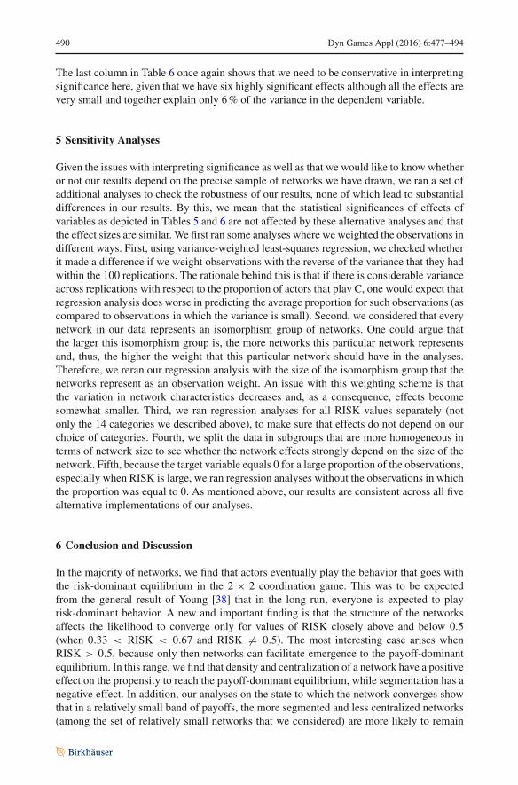
Fig. 1 Effects of network characteristics on the average proportion of actors playing the payoff-dominantequilibrium for fourteen RISK categories. Effect size shows how much the likelihood of reaching the payoff-dominant equilibrium increases with a one-unit increase in the related independent variable for a specificRISK category. Note that the scale on the x-axis is not linear in RISK, because the RISK categories are notequidistant (cf. Table 3)

moving to the risk-dominant equilibrium reduces quickly. Finally, we graph the regressioncoefficients of the six network characteristics in Fig. 1, where the analyses are done for eachRISK category separately. This figure shows that in particular in the first 10 RISK categories,the effects changewithRISK, butmostly stay consistently either positive or negative (networksize is the exception). The figure also demonstrates again that the network effects decreasedramatically if RISK is larger than 2/3. All the network effects also seem to start decreasingfor RISK approaching 0.5. Note that in all likelihood, this is not a spurious effect, since allnetwork effects are 0 at RISK = 0.5.

In Table 6, we show three regression analyses predicting the probability to converge toa state in which behavior is heterogeneous.8 As was shown in Table 3, this probability isalways low. Surprisingly, there is hardly any effect of density on expected heterogeneity ofbehavior, and it shows a pattern that is difficult to interpret. Given the problems to interpretsignificance in these simulated data and the relatively low t values for the coefficient, wemaintain the claim that there is hardly any evidence to support a substantial effect of densityhere. By far, the most important predictor is segmentation of the network, and it has, asexpected, a positive effect on persistent heterogeneity of behavior. The proportion of actorswith an odd number of neighbors also has a substantial positive effect. Centralization has aconsistent negative effect on heterogeneity of behavior. Again, both the size of the networkand the maximal degree of the network have small and difficult to interpret effects. Given thatthese hardly contribute to the explained variance, we will not try to interpret them in moredetail. As in Table 5, we see that the explained variance decreases with increasing RISK.

8 Again the results do not change substantially when we first logit-transform the target variable.

490 Dyn Games Appl (2016) 6:477–494

The last column in Table 6 once again shows that we need to be conservative in interpretingsignificance here, given that we have six highly significant effects although all the effects arevery small and together explain only 6% of the variance in the dependent variable.

5 Sensitivity Analyses

Given the issues with interpreting significance as well as that we would like to know whetheror not our results depend on the precise sample of networks we have drawn, we ran a set ofadditional analyses to check the robustness of our results, none of which lead to substantialdifferences in our results. By this, we mean that the statistical significances of effects ofvariables as depicted in Tables 5 and 6 are not affected by these alternative analyses and thatthe effect sizes are similar. We first ran some analyses where we weighted the observations indifferent ways. First, using variance-weighted least-squares regression, we checked whetherit made a difference if we weight observations with the reverse of the variance that they hadwithin the 100 replications. The rationale behind this is that if there is considerable varianceacross replications with respect to the proportion of actors that play C, one would expect thatregression analysis does worse in predicting the average proportion for such observations (ascompared to observations in which the variance is small). Second, we considered that everynetwork in our data represents an isomorphism group of networks. One could argue thatthe larger this isomorphism group is, the more networks this particular network representsand, thus, the higher the weight that this particular network should have in the analyses.Therefore, we reran our regression analysis with the size of the isomorphism group that thenetworks represent as an observation weight. An issue with this weighting scheme is thatthe variation in network characteristics decreases and, as a consequence, effects becomesomewhat smaller. Third, we ran regression analyses for all RISK values separately (notonly the 14 categories we described above), to make sure that effects do not depend on ourchoice of categories. Fourth, we split the data in subgroups that are more homogeneous interms of network size to see whether the network effects strongly depend on the size of thenetwork. Fifth, because the target variable equals 0 for a large proportion of the observations,especially when RISK is large, we ran regression analyses without the observations in whichthe proportion was equal to 0. As mentioned above, our results are consistent across all fivealternative implementations of our analyses.

6 Conclusion and Discussion

In the majority of networks, we find that actors eventually play the behavior that goes withthe risk-dominant equilibrium in the 2 × 2 coordination game. This was to be expectedfrom the general result of Young [38] that in the long run, everyone is expected to playrisk-dominant behavior. A new and important finding is that the structure of the networksaffects the likelihood to converge only for values of RISK closely above and below 0.5(when 0.33 < RISK < 0.67 and RISK �= 0.5). The most interesting case arises whenRISK > 0.5, because only then networks can facilitate emergence to the payoff-dominantequilibrium. In this range, we find that density and centralization of a network have a positiveeffect on the propensity to reach the payoff-dominant equilibrium, while segmentation has anegative effect. In addition, our analyses on the state to which the network converges showthat in a relatively small band of payoffs, the more segmented and less centralized networks(among the set of relatively small networks that we considered) are more likely to remain

Dyn Games Appl (2016) 6:477–494 491

heterogeneous. Network density does not have an effect on the likelihood of behavior toconverge to a homogenous state.

The important advantage compared to earlierwork is thatwe identify a set of network char-acteristics that affect coordination behavior in networks while controlling for simultaneouslyvarying other network characteristics. Santos et al.’s [28] finding that efficient coordination ismore likely in heterogeneous networks is in line with our finding that centralization promotesefficient coordination, but we show that other types of heterogeneity in the network, such assegmentation, can have negative effects on reaching efficient coordination. Our results alsoprovide alternative explanations for why previous theoretical papers in which sets of largenetworks are compared often do not find network effects (cf. [25–27,30]). As we show forsmaller networks, network effects are relevant only in a limited part of the payoff parame-ter space, but in this space, they do exist. In most of the papers comparing sets of (large)networks, a large range of payoffs is considered and when one compares results across thiswhole parameter space, network effects might indeed appear small or nonexistent. A secondalternative explanation is that in the papers in this tradition, usually a few sets of networksare compared, for instance, scale-free networks and regular lattices, while the structuraldifferences between these networks are multi-dimensional. Clearly, scale-free networks aremore centralized than regular lattices, but they could also be more segmented (or differ inother network characteristics). Given that these two structural network characteristics haveopposing effects according to our analyses, these two effects might cancel out by comparinga set of scale-free networks with a set of regular lattices. On the other hand, any differencesfound between, say, scale-free networks and regular lattices could have been due to multipledifferences in characteristics of the network structure. We consider the identification of thisissue as one of the main steps ahead of this contribution.

The positive effect of density on reaching the payoff-dominant equilibrium is consistentwith the neighborhood size effect found in Berninghaus and Schwalbe [5] because in theirmodels, a network is denser if neighborhood size increases. Our model gives a somewhatmore elaborate underpinning of this effect in Berninghaus and Schwalbe [5], as in their case,their result was based on a restricted set of networks (only lattices were considered). There arealso some notable differences with previous research in terms of predictions for empiricaltests. Given that our model predicts that networks with odd neighborhood sizes are morelikely to evolve to the payoff-dominant equilibrium than networks with even neighborhoodsizes, we predict that the effect of neighborhood size is not monotonic. For instance, giventhe coefficients in our model, we predict that three-person neighborhoods converge to thepayoff-dominant equilibrium more easily than four-person neighborhoods. Unfortunately,this result cannot be tested with the kinds of experiments as reported in Berninghaus et al.[4], because, probably coincidentally, only even-numbered neighborhoods were used in thatcase.

Comparing our resultsmore closelywith the experimental results byBerninghaus et al. [4],it is striking that although they use a rather high RISK value (0.7), they do find convergenceto the payoff-dominant equilibrium as well as large differences between network conditions.This contrastswith our theoretical finding that the differences between networksmainly occurat RISK values between 0.5 and 0.6. One potential explanation for this is that our simulation isbased on actors who start to make random choices, while subjects in the laboratory might usestarting propensities with a higher weight on playing the payoff-dominant-related behavior.An alternative explanation is that introducing altruism in the model by placing at least somepositive weight on the payoff for the other person in a utility function of this person wouldalready decrease the RISK value of the game in terms of utility (as compared to in termsof only the payoffs). Therefore, it may be reasonable for comparing our results with these

492 Dyn Games Appl (2016) 6:477–494

and future experimental results to assume that the subjective risk for the participants to playthe payoff-dominant equilibrium is lower than if one would purely consider the payoffs. Aswe mentioned in the introduction, Berninghaus et al. [4] also find that the payoff-dominantequilibrium is reached more easily in the closed triad than in the circle with eight actors.The main variation here is the change in the density of the network and this result clearlycorresponds with the positive effect we find for density on reaching the payoff-dominantequilibrium. When one compares a lattice in which everybody plays with four neighbors,with a circle where subjects also play with four neighbors (both networks with a total of 16nodes), the only network characteristic that varies is segmentation. Density, centralization,etc., are all constant. Our positive effect of segmentation for intermediate risk values couldexplain the higher probability of subjects playing C on the circle. Of course, this cannot beconsidered as conclusive evidence for our theory given that the subjective risk is unclear andthe effect of segmentation also changes depending on the value of RISK. Nevertheless, ourtheoretical results seem to have at least some consistency with these empirical results.

The fact that network effects are limited to the range of payoffs where there is a slightlystronger attraction of the risk-dominant equilibrium than of the payoff-dominant equilibrium(or the other way round) might also be the explanation why Antonioni et al. [2] do not findan effect of cliquish (segmented) networks on convergence to the payoff or risk-dominantequilibrium and Frey et al. [15] do not find the network effects that are expected from ouranalyses. Again one issue might be that the subjective risk is not the same as the risk weconsider purely based on monetary payoffs. A strong argument in favor of this explanationis that the payoff-dominant equilibrium remains a strong attractor even with RISK is con-siderably larger than 0.5. Both papers blame deviations from theoretical predictions alsoon the assumption of myopic best reply behavior and suggest that subjects might use moresophisticated behavioral strategies. Although in general we would prefer to stick to the moresimple behavioral theory, we concede that making the behavioral assumptions more complexis an equally promising strand for further research in trying to understand the dynamics ofcoordination on networks better.

Besides the comparisonwith existing empirical research, we provide several new hypothe-ses on effects of network characteristics on both the playing behavior related to the payoff-dominant equilibrium and the likelihood that multiple norms persist after convergence. Test-ing some of these hypotheses empirically remains a challenge for future research. A likelytheoretical extension would be to consider how conclusions would change if we do not onlyallow actors to change their ties but also to change their partners. For an overview on theliterature on these dynamic networks, one can consult Dutta and Jackson [13]. Specific mod-els on coordination games played on networks are studied by Jackson and Watts [19], Goyaland Vega-Redondo [17], Berninghaus and Vogt [6], Buskens et al. [8] and Tsvetkova andBuskens [31].

Acknowledgments We thank Siegfried Berninghaus, Werner Raub, Tom Snijders and Jeroen Weesie fortheir comments and suggestions on earlier versions of this manuscript. This paper is part of the Polarization andConflict Project CIT-2-CT-2004-506084 funded by the European Commission-DGResearch Sixth FrameworkProgramme. This article reflects only the author’s views, and the Community is not liable for any use that maybe made of the information contained therein. Financial support for Buskens was provided by the RoyalNetherlands Academy of Arts and Sciences (KNAW) for the project ‘Third-Party Effects in CooperationProblems’ and by Utrecht University for the High Potential-program ‘Dynamics of Cooperation, Networks,and Institutions.’

Open Access This article is distributed under the terms of the Creative Commons Attribution License whichpermits any use, distribution, and reproduction in any medium, provided the original author(s) and the sourceare credited.

Dyn Games Appl (2016) 6:477–494 493

Appendix: Sampling of Networks

Below you find a more detailed account of the number and kind of networks sampled.The networks are available for research purposes. For network sizes from 2 through 8, weuse all connected non-isomorphic networks (N = 12,112). Networks are generated usingspecialized software called Nauty version 2.2 (see [22]).

For networks size 9 through 25, we use all the connected non-isomorphic networks fordensities (number of ties) for which the number of different networks is limited. For otherdensities, we choose a random sample of the connected networks, where random means thateach tie had the same probability of being in the network.

In detail:

• Size 9: all networks with 8–10 or 26–36 ties; sample of 400 for networks with 11–25ties.

• Size 10: all networks with 9–10 or 36–45 ties; sample of 300 for networks with 11–35ties.

• Size 11: all networks with 10–11 or 46–55 ties; sample of 200 for networks with 12–45ties.

• Size 12: all networks with 11 or 57–66 ties; sample of 200 for networks with 12–56 ties.• Size 13: all networks with 69–78 ties; sample of 50 for networks with 12–68 ties.• Size 14: all networks with 82–91 ties; sample of 50 for networks with 13–81 ties.• Size 15: all networks with 96–105 ties; sample of 50 for networks with 14–95 ties.• Size 16: all networks with 111–120 ties; sample of 50 for networks with 15–110 ties.• Size 17–25:

• all networks with size · (size − 1)/2 to size · (size − 1)/2 − 5 ties.• sample of 20 for networks with size −1 to size · (size − 1) − 6 ties.

Total number of networks: 112,614.

References

1. Anderlini L, IanniA (1996) Path dependence and learning fromneighbors. GameEconBehav 13:141–1772. AntonioniA,CacaultMP, LaliveR, TomassiniM (2013)Coordination on networks: does topologymatter?

PLoS One 8(2):e550333. Baerveldt C, Snijders TAB (1994) Influences on and from the segmentation of networks: hypotheses and

tests. Soc Netw 16:213–2324. Berninghaus SK, Ehrhart K-M,Keser C (2002) Conventions and local interaction structures: experimental

evidence. Game Econ Behav 39:177–2055. Berninghaus SK, Schwalbe U (1996) Conventions, local interaction and automata networks. J Evol Econ

6:313–3246. Berninghaus SK, Vogt B (2006) Network formation in symmetric 2×2 games. Homo Oecon 23:421–4667. Buskens V (2002) Social networks and trust. Kluwer, Boston8. Buskens V, Corten R, Weesie J (2008) Consent and conflict: coevolution of coordination and networks.

J Peace Res 45:205–2229. BuskensV,YamaguchiK (1999)A newmodel for information diffusion in heterogeneous social networks.

In: Becker M, Sobel M (eds) Sociological methodology. Blackwell, Oxford, pp 281–32510. Cassar A (2007) Coordination and cooperation in local, random and small world networks: experimental

evidence. Games Econ Behav 58:209–23011. Coleman JS (1988) Social capital in the creation of human capital. Am J Soc 94:S95–S12012. Cooper R, DeJong D, Forsythe R, Ross TW (1990) Selection criteria in coordination games: some exper-

imental results. Am Econ Rev 80:218–23413. Dutta B, Jackson MO (eds) (2003) Networks and groups: models of strategic formation. Springer, Berlin14. Ellison G (1993) Learning, local interaction, and coordination. Econometrica 61:1047–1071

494 Dyn Games Appl (2016) 6:477–494

15. FreyV,CortenR,BuskensV (2012)Equilibriumselection in network coordinationgames: an experimentalstudy. Rev Netw Econ 11(3). doi:10.1515/1446-9022.1365

16. Friedman D (1996) Equilibrium in evolutionary games: some experimental results. Econ J 106:1–2517. Goyal S, Vega-Redondo F (2005) Network formation and social coordination. Game Econ Behav 2:178–

20718. Harsanyi JC, Selten R (1988) A general theory of equilibrium selection in games. MIT Press, Cambridge19. JacksonMO,Watts A (2002) On the formation of interaction networks in social coordination. Game Econ

Behav 41:265–29120. KandoriM,MailathGJ, RobR (1993) Learning,mutation, and long run equilibria in games. Econometrica

61:29–5621. Keser C, Erhart KM, Berninghaus S (1998) Coordination and local interaction: experimental evidence.

Econ Lett 59:269–27522. McKay BD (2003) Nauty user’s guide (version 2.2). Tech. Rpt. TR-CS-90-02, Dept. Computer Science,

Australian National University23. Nowak MA, May RM (1992) Evolutionary games and spatial chaos. Nature 359:826–82924. Raub W, Weesie J (1990) Reputation and efficiency in social interactions: an example of network effects.

Am J Soc 96:626–65425. Roca CP, Cuesta JA, Sánchez A (2009a) Effect of spatial structure on the evolution of cooperation. Phys

Rev E 80:04610626. RocaCP,Cuesta JA, SánchezA (2009b) Promotion of cooperation on networks?Themyopic best response

case. Eur Phys J B Condens Matter Complex Syst 71:587–59527. Roca CP, Lozano S, Arenas A, Sánchez A (2010) Topological traps control flow on real networks: the

case of coordination failures. PLoS One 5(12):e1521028. Santos FC, Pacheco JM, Lenaerts T (2006) Evolutionary dynamics of social dilemmas in structured

heterogeneous populations. PNAS 103:3490–349429. Snijders TAB (1981) The degree variance: an index of graph heterogeneity. Soc Netw 3:163–17430. Tomassini M, Pestelacci E (2010) Evolution of coordination in social networks: a numerical study. Int J

Mod Phys C 21(10):1277–129631. Tsvetkova M, Buskens V (2013) Coordination on egalitarian networks from asymmetric relations in a

social game of chicken. Adv Complex Syst 16(1): doi:10.1142/S021952591350005732. VanHuyck JB (2008) Emergent conventions in evolutionary games. In: Plott CR, Smith S (eds) Handbook

of experimental economics results. North Holland, Amsterdam, pp 520–53033. Van Huyck JB, Battalia RC, Beil RO (1990) Tacit coordination, strategic uncertainty, and coordination

failure. Am Econ Rev 80:234–24834. Van Huyck JB, Battalia RC, Beil RO (1991) Strategic uncertainty, equilibrium selection, and coordination

failure. Q J Econ 106:885–91035. Wasserman S, Faust K (1994) Social network analysis: methods and applications. Cambridge University

Press, New York36. Yamaguchi K (1994) The flow of information through social networks: diagonal-free measures of ineffi-

ciency and the structural determinants of inefficiency. Soc Netw 16:57–8637. Young HP (1993) The evolution of conventions. Econometrica 61:57–8438. YoungHP (1998) Individual strategy and social structure: an evolutionary theory of institutions. Princeton

University Press, Princeton