EFFECTS OF LANDSCAPE CONFIGURATION ON NORTHERN …

EFFECTS OF LANDSCAPE CONFIGURATION ON NORTHERN BOBWHITE IN

SOUTHEASTERN KANSAS

by

BRIAN E. FLOCK

B.S., California University of Pennsylvania, 1997 M. S., Emporia State University, 2002

AN ABSTRACT OF A DISSERTATION

submitted in partial fulfillment of the requirements for the degree

DOCTOR OF PHILOSOPHY

Division of Biology College of Arts and Sciences

KANSAS STATE UNIVERSITY Manhattan, Kansas

2006

Abstract

Northern bobwhite (Colinus virginianus) populations in much of the species range have been

declining for the last 35 years. I trapped and equipped bobwhite with radio transmitters and

tracked them during 2003-2005. I used these data to examine the effects of landscape

configuration on survival as well as the habitat association of bobwhite in southeastern Kansas. I

used the nest survival model in Program MARK to determine the effects of habitat configuration

on weekly survival of radio equipped bobwhite during the Fall-Spring (1 October to 14 April)

and the Spring-Fall (15 April to 30 September) at home range and 500 m buffer scales.

Individual survival probability for the Fall-Spring period was 0.9439 (S.E. = 0.0071), and the

most parsimonious model for the Fall-Spring period at the home range scale was B0 + percent

woodland + percent cropland. At the 500 m buffer scale the most parsimonious model was B0 +

percent Conservation Reserve (CRP) program land. The weekly survival probability for the

Spring-Fall period was 0.9559 (S.E. = 0.0098). At the home range and 500 m buffer scales there

were weak associations of habitat to survival during Spring-Fall with the most parsimonious

model for both scales B0 + percent other. Using Euclidean Distances to measure distance from

animal location to each habitat, I found that habitat selection was occurring during the Spring-

Fall (Wilkes λ = 0.04, F 6,36 = 143.682, P < 0.001) and Fall-Spring (Wilkes λ = 0.056, F 6, 29 =

81.99, P < 0.001). During Spring-Fall bobwhite were associated with locations near cool-season

grasses and during Fall-Spring preferred locations near woody cover. Bobwhite also showed

habitat selection at a second more refined land use classification level for Spring-Fall (Wilkes λ

= 0.006, F 16, 26 = 284.483, P < 0.001) and Fall-Spring (Wilkes λ = 0.004, F 16, 19 = 276.037, P <

0.001). During the Spring-Fall, bobwhites were associated with locations near cool-season grass

pastures and roads and during Fall-Spring were associated with locations in close proximity to

roads and CRP. Understanding the effects of habitat configuration on bobwhite is an important

step in developing a broad-scale management plan.

EFFECTS OF LANDSCAPE CONFIGURATION ON NORTHERN BOBWHITE IN

SOUTHEASTERN KANSAS

by

BRIAN E. FLOCK

B. S., California University of Pennsylvania, 1997 M.S., Emporia State University, 2002

A DISSERTATION

submitted in partial fulfillment of the requirements for the degree

DOCTOR OF PHILOSOPHY

Division of Biology College of Arts and Sciences

KANSAS STATE UNIVERSITY Manhattan, Kansas

2006

Approved by:

Major Professor Dr. Philip S. Gipson

Abstract

Northern bobwhite (Colinus virginianus) populations in much of the species range have

been declining for the last 35 years. I trapped and equipped bobwhite with radio transmitters and

tracked them during 2003-2005. I used these data to examine the effects of landscape

configuration on survival as well as the habitat association of bobwhite in southeastern Kansas. I

used the nest survival model in Program MARK to determine the effects of habitat configuration

on weekly survival of radio equipped bobwhite during the Fall-Spring (1 October to 14 April)

and the Spring-Fall (15 April to 30 September) at home range and 500 m buffer scales.

Individual survival probability for the Fall-Spring period was 0.9439 (S.E. = 0.0071), and the

most parsimonious model for the Fall-Spring period at the home range scale was B0 + percent


percent Conservation Reserve (CRP) program land. The weekly survival probability for the

Spring-Fall period was 0.9559 (S.E. = 0.0098). At the home range and 500 m buffer scales there

were weak associations of habitat to survival during Spring-Fall with the most parsimonious

model for both scales B0 + percent other. Using Euclidean Distances to measure distance from

animal location to each habitat, I found that habitat selection was occurring during the Spring-

Fall (Wilkes λ = 0.04, F 6,36 = 143.682, P < 0.001) and Fall-Spring (Wilkes λ = 0.056, F 6, 29 =

81.99, P < 0.001). During Spring-Fall bobwhite were associated with locations near cool-season

grasses and during Fall-Spring preferred locations near woody cover. Bobwhite also showed

habitat selection at a second more refined land use classification level for Spring-Fall (Wilkes λ

= 0.006, F 16, 26 = 284.483, P < 0.001) and Fall-Spring (Wilkes λ = 0.004, F 16, 19 = 276.037, P <

0.001). During the Spring-Fall, bobwhites were associated with locations near cool-season grass

pastures and roads and during Fall-Spring were associated with locations in close proximity to

roads and CRP. Understanding the effects of habitat configuration on bobwhite is an important

step in developing a broad-scale management plan.

Table of Contents

List of Figures .................................................................................................................... iii

List of Tables ..................................................................................................................... iv

Acknowledgements........................................................................................................... vii

CHAPTER 1 - Introduction ................................................................................................ 1

CHAPTER 2 - Effects of Landscape Configuration on Northern Bobwhite Survival ....... 2

Abstract........................................................................................................................... 2

Introduction..................................................................................................................... 2

Study Area ...................................................................................................................... 4

Methods .......................................................................................................................... 5

Survival ....................................................................................................................... 7

Survival Habitat Analysis ........................................................................................... 7

Results............................................................................................................................. 8

Discussion....................................................................................................................... 9

Management Implications............................................................................................. 12

CHAPTER 3 - Distance – Based Habitat Associations of Northern Bobwhite in

Southeastern Kansas ......................................................................................................... 30

Abstract......................................................................................................................... 30

Introduction................................................................................................................... 31

Study Area .................................................................................................................... 32

Methods ........................................................................................................................ 33

Habitat Association Analysis .................................................................................... 34

Results........................................................................................................................... 35

Land Cover Analysis................................................................................................. 36

Land Use Analysis .................................................................................................... 36

Discussion..................................................................................................................... 37


CHAPTER 4 - A Technique for Modeling Usable Space Based on Distance.................. 48

Abstract......................................................................................................................... 48

i

Introduction................................................................................................................... 48

Study Area .................................................................................................................... 50

Methods ........................................................................................................................ 50

Results........................................................................................................................... 51

Discussion..................................................................................................................... 51


CHAPTER 5 - A Blueprint for Northern Bobwhite Habitat Management in the Modern

Agricultural Landscape..................................................................................................... 69

Abstract......................................................................................................................... 69

Introduction................................................................................................................... 69

Habitat Management: A Multiple Scale Approach....................................................... 71

Broad-scale Planning ................................................................................................ 71

Focus Area Planning and Management .................................................................... 73

Thinking Outside the Box: Biofuels and Wildlife Habitat ........................................... 75

Conclusions................................................................................................................... 76

CHAPTER 6 - Summary and Conclusions....................................................................... 78

CHAPTER 7 - References ................................................................................................ 80

ii

List of Figures

Figure 2.1. Weekly survival probabilities for southeastern Kansas, USA, with upper (---) and

lower (···) confidence intervals for northern bobwhite based on most parsimonious model,

B0 + percent CRP, during the Fall-Spring (1 October to 30 September) at the 500 m buffer

scale....................................................................................................................................... 26

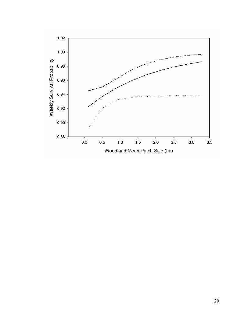
Figure 2.2. Weekly survival probabilities for southeastern Kansas, USA, with upper (---) and

lower (···) confidence interval for northern bobwhite based on second most parsimonious

model, B0 + Woodland Mean Patch Size, during the Fall-Spring (1 October to 14 April) at

the 500 m buffer scale........................................................................................................... 28

Figure 4.1. 2003 land cover of study area in southeastern Kansas, USA. ................................... 55

Figure 4.2. Winter weighted overlay model based on 5 habitat categories and 30-150m buffers

around each habitat to depict October to April usable space in southeastern, Kansas, USA.

............................................................................................................................................... 57

Figure 4.3. October to April usable space model with known covey locations in a portion of

southeastern Kansas, USA. ................................................................................................... 59

Figure 4.4. 2003 land cover of a portion study area in southeast Kansas, USA, containing a large

Conservation Reserve Program field before hypothetical management............................... 61

Figure 4.5. October-April usable space model based on 5 habitat categories and distance from

each habitat before hypothetical management on study area in southeastern, Kansas, USA.

............................................................................................................................................... 63

Figure 4.6. Portion of study area in southeastern Kansas, USA, with hypothetical management in

place which include fencerows and native warm season grass buffers. ............................... 65

Figure 4.7. October to April usable space model based on hypothetically managed portion of

study area in southeastern, Kansas, USA, based on 5 habitat categories and distance to each

habitat.................................................................................................................................... 67

iii

List of Tables

Table 2.1. Percentage of land cover classes found in the study area in southeastern Kansas,

USA, 2003 to 2005. .............................................................................................................. 14

Table 2.2. Model selection for weekly probability of individual survival based on habitat

configuration of the covey home range during Fall-Spring (1 October to 14 April) for

northern bobwhite in southeastern Kansas, USA, 2003 to 2005. Model statistics include the

deviance (Dev -2lnℓ), number of parameters (K), Akaike’s Information Criterion (AICc)

corrected for small sample sizes, ∆ AICc, and Akaike weights (wi). Presented are the top 20

models. .................................................................................................................................. 15

Table 2.3. Model selection for weekly probability of individual survival based on habitat

configuration of 500 m buffer around covey home range during Fall-Spring (1 October to

14 April) for northern bobwhite in southeastern Kansas, USA, 2003 to 2005. Model

statistics include the deviance (Dev -2lnℓ), number of parameters (K), Akaike’s Information

Criterion (AICc) corrected for small sample sizes, ∆ AICc, and Akaike weights (wi).

Presented are the top 20 models............................................................................................ 17

Table 2.4. Observed and hypothetical habitat configurations based on B0 + percent woodland +

percent cropland and their effects on probability of weekly survival (Sw) and standard error

(SE) during the Fall-Spring (1 October to 14 April) at the home range scale in southeastern

Kansas, USA. ........................................................................................................................ 19

Table 2.5. Observed and hypothetical habitat configurations based on B0 + percent woodland +

percent CRP and their effects on probability of weekly survival (Sw) and standard error (SE)

during the Fall-Spring (1 October to 14 April) at the home range scale in southeastern

Kansas, USA. ........................................................................................................................ 20

Table 2.6. Model selection for comparison of burned CRP versus nonburned CRP individual

weekly probability of surviving for northern bobwhite in southeastern Kansas, USA, 2003

to 2005 during Fall-Spring (1 October to 14 April). Model statistics include the deviance

(Dev -2lnℓ), number of parameters (K), Akaike’s Information Criterion (AICc) corrected for

small sample sizes, ∆ AICc, and Akaike weights (wi). ......................................................... 21

Table 2.7. Model selection for weekly probability of surviving based on habitat configuration of

home range scale during Spring-Fall (a5 April to 30 September) for northern bobwhite in

iv

southeastern Kansas, USA, 2003 to 2005. Model statistics include the deviance (Dev -

2lnℓ), number of parameters (K), Akaike’s Information Criterion (AICc) corrected for small

sample sizes, ∆ AICc, and Akaike weights (wi). Presented are the top 25 models............... 22

Table 2.8. Model selection for weekly probability of surviving based on habitat configuration of

500 m buffer during Spring-Fall (15 April to 30 September) for northern bobwhite in

southeastern Kansas, USA, 2003 to 2005. Model statistics include the deviance (Dev -

2lnℓ), number of parameters (K), Akaike’s Information Criterion (AICc) corrected for small

sample sizes, ∆ AICc, and Akaike weights (wi). Presented are the top 20 models............... 24

Table 3.1. Percentage of level 2 land use classes from 2003 to 2005 for the study in southeastern

Kansas, USA. ........................................................................................................................ 41

Table 3.2. Pair-wise comparisons of distance/random ratios for habitats for southeastern Kansas,

USA, during Spring-Fall (15 April to 30 September) at the level 1 land cover classification

scheme. Table shows t-value (p-value) for each pair-wise comparison along with final land

cover ranking. The higher the rank more preference for that land cover type...................... 42

Table 3.3. Pair-wise comparisons of distance/random ratios for habitats in southeastern Kansas,

USA, during Fall-Spring (1 October to 14 April) at the level 1 land cover classification

scheme . Table shows t-value (p-value) for each pair-wise comparison along with final

ranking. The higher the rank more preference for that land cover type. .............................. 43

Table 3.4. Simplified ranking matrices based on pair-wise comparisons of distance/random

ratios for each land use class during Spring-Fall (15 April to 30 September). Each element

in the matrix was replaced by its sign; a triple sign represents significant difference at the P

< 0.05. A + represents a positive association and a – represents a negative association. The

higher the rank more preference for that land use type. ....................................................... 44

Table 3.5. Simplified ranking matrices based on pair-wise comparisons of distance/random

ratios for each land use class during Fall-Spring (1 October to 14 April). Each element in

the matrix was replaced by its sign; a triple sign represents significant difference at the P <

0.05. A + represents a positive association and a – represents a negative association. The

higher the rank more preference for that land usetype. ........................................................ 46

Table 4.1. Model values used to create October-April weighted overlay analysis of usable space

available for northern bobwhite in my study area in southeast Kansas, USA. Percentages

v

are based on proportion of telemetry locations for bobwhite within each habitat. A higher

score represents a more favorable area for bobwhite............................................................ 54

vi

Acknowledgements

First, I thank my adviser Dr. Philip S. Gipson for giving me the opportunity to work on

this research with him. He has shown immeasurable patience and support through out my tenure

at Kansas State University. I would also like to thank Roger D. Applegate for being a mentor

and friend. He has shown great patience, support, and kindness over the last 8 years and in

particular over the last 2 years. With his guidance and tutelage I became a better biologist and

researcher. I would like to thank my other committee members Brett K. Sandercock, Shawn J.

Hutchinson, and Warren Ballard for serving on my committee and providing advice and support.

From Kansas Department of Wildlife and Parks (KDWP), I would like to thank Lance

Hedges for providing assistance on the project and providing me landowner contacts in

southeastern Kansas. I would also like to thank the numerous conservation officers and biologists

in the Region 5 who helped fill in during the brief period when I was without a Research

Assistant.

I would like to thank Frank Loncarich and Tracy Dick for helping me with fieldwork and

collecting data used in my dissertation. I particularly thank Tim Strakosh for filling in during my

last summer of data collection even though he was working on his own dissertation. I also thank

the numerous landowners for allowing me to conduct my research on their property. Without

them this research would not have been conducted.

Much love and support was provided by my Father, Mother, sister, Lorraine Koontz and

brother-in-law Duane Koontz.

The funding source for this research was CFDA Wildlife Restoration Federal Act 15.611,

Kansas Department of Wildlife and Parks Federal Aid Grant W-50-R-4. Additional funding was

provided by KSU Division of Biology, Kansas State University, U. S. Geological Survey, and

The Wildlife Management Institute.

vii

CHAPTER 1 - Introduction

Northern bobwhite (Colinus virginianus) populations have shown a declining trend for

the last 35+ years throughout much of their range (Sauer et al. 2005) even though the bobwhite is

one of the most studied game birds in North America. This decline has often been attributed to

changes in land-use, particularly changes in farming practices (Brennan 1991, Church and Taylor

1992, Brady et al.1993, Peterson et al. 2002). The shift to clean farming resulted in a loss of

habitat as well as fragmentation of the landscape.

In order to improve quail habitat, past management has focused on enhancing habitat

quality at a fine scale such as a field. Under this plan it is assumed that “quality habitat”

randomly scattered throughout the landscape will provide increased numbers of quail and other

wildlife. Often the benefits of this type of management are backed up by the use of correlative

measures such as density or use versus availability studies. Van Horne (1983) felt that density

was a misleading indicator of habitat quality and listed environmental and species specific

characteristics that increased the probability that density would not be correlated positively with

habitat quality. Other researchers have concluded that use versus availability were poor measures

of habitat quality. Hobbs and Hanley (1990) concluded that use versus availability revealed little

about habitat quality and recommended using studies which enabled investigation of direct links

between habitat and an organism’s fitness. One way to link habitat quality to fitness is by

examining the effects of habitat on the organism’s survival (Garshelis 2000).

Edge has been hypothesized to be an important habitat component for bobwhite

(Stoddard 1931, Rosene 1984). However, very little information is available on the preference of

bobwhite for various edge types or what constitutes acceptable edge. Roseberry and Sudkamp

(1998) found that Illinois bobwhites were associated with patchy landscapes that contained

moderate amounts of row crop, grassland, and abundant woody edge.

My objectives for this study were to determine 1) the effects of landscape configuration

in a fescue dominated agricultural system on bobwhite survival and habitat preference; 2) to

develop a spatial model for determining usable space within the landscape; and 3) develop a

blueprint for managing northern bobwhite within the modern agricultural landscape.

1

CHAPTER 2 - Effects of Landscape Configuration on Northern

Bobwhite Survival

Abstract Northern bobwhite (Colinus virginianus) populations in much of the species range have been

declining for the last 35+ years. This decline has continued, even though northern bobwhites are

one of the most studied and managed game birds in North America. Past work has often focused

on fine-scale management and research often at the field scale. Also the benefits of fine-scale

management have often been based on density and habitat use versus availability studies. A

better method is to relate habitat use to fitness: either survival or reproductive success. I used

the nest survival model in Program MARK to determine the effects of habitat configuration on

weekly survival of radio equipped bobwhite during the Fall-Spring (1 October to 14 April) and

the Spring-Fall (15 April to September 30) at home range and 500 m buffer scales. Individual

survival probability for the Fall-Spring period was 0.9439 (S.E. = 0.0071). The most

parsimonious model for the Fall-Spring period at the home range scale was B0 + percent


percent Conservation Reserve (CRP) program land. Percent woodland and percent cropland were

positively associated while percent CRP was negatively associated with Fall-Spring survival.

The weekly survival probability for the Spring-Fall period was 0.9559 (S.E. = 0.0098). At the

home range and 500 m buffer scales there were weak associations of habitat to survival during

Spring-Fall. The most parsimonious model for both scales was B0 + percent other, but it was

equally parsimonious to the Null model (no covariates and constant survival). Understanding the

effects of habitat configuration on northern bobwhite is an important step in developing a broad

scale management plan for northern bobwhite. During the Fall-Spring period when habitat may

be more limited in areas dominated by fescue increasing woodland habitat particularly shrub

cover in close proximity to cropland areas should increase survival.

Introduction Northern bobwhite (Colinus virginianus) populations have shown a declining trend for

the last 35+ years throughout much of their range (Sauer et al. 2005) even though the bobwhite is

one of the most studied game birds in North America. The decline has often been attributed to

2

changes in land use, particularly changes in farming practices (Brennan 1991, Church and Taylor

1992, Brady et al.1993, Peterson et al. 2002). The shift to clean farming resulted in a loss of

habitat as well as fragmentation of the landscape.

In order to improve bobwhite habitat past management has focused on enhancing habitat

quality at a fine scale such as a field. Management at this level may include food plots, disk

strips, planting of native warm season grasses, or prescribed burning. Under this plan it is

assumed that “quality habitat” randomly scattered through out the landscape will provide

increased numbers of quail and other wildlife. Often the benefits of this type of management are

inferred from the use of correlative measures such as density or use versus availability studies.

However density measures may not be adequate for measuring the responses of quail or other

wildlife to habitat improvements.

Van Horne (1983) felt that density was a misleading indicator of habitat quality and

listed environmental and species specific characteristics that increase the probability that density

would not be correlated positively with habitat quality. The environmental characteristics include

highly seasonal habitat requirements, unpredictability over time, and patchiness of habitat (Van

Horne 1983). Species characteristics include having social dominance interactions, high Spring-

Fall capacity, and being generalist (Van Horne 1983). Both the environmental and species

characteristics describe the life history of quail especially in the current agricultural landscape.

The problem with considering only density while ignoring these traits of quail is that habitat

management limited to a fine spatial scale can result in doing more harm than good. For instance

if density is used to measure the relative quality of a particular habitat, biologists may be

ignoring source/sink dynamics that could be occurring in the area. The alteration of habitat

could result in high density of individuals in the altered patch while numbers are depressed in the

surrounding area. However, if the high density of individuals is not due to high fitness, but

instead the result of individuals being drawn into the area and resulting lower fitness, the

assumptions that the habitat is quality habitat is violated.

Other researchers have concluded that use versus availability were poor measures of

habitat quality. Hobbs and Hanley (1990) concluded that use versus availability revealed little

about habitat quality and recommended using studies which enabled investigation of direct links

between habitat and an organism’s fitness. One way to link habitat quality to fitness is by

examining the effects of habitat on the organism’s survival (Garshelis 2000).

3

Habitat use and survival have been studied extensively, but specific linkages between

habitat quality and survival have not been established. For instance, Williams et al. (2000) felt

that survival, movement, and woody-cover selection seemed to be linked on their rangeland

study. Taylor et al. (1999) also felt that habitat composition probably affected survival, but they

were unable to establish direct linkages or make specific recommendations. More often survival

and habitat have been treated as two separate entities as reported by Dixon et al. (1996). Call

(2002) did attempt to determine the effects of habitat on survival; however her models indicated

that behavior such as nesting or brood rearing had significant affects on survival.

Another problem with past research was that it often focused on relatively fine temporal

scales during the life cycle of northern bobwhite. For instance some studies either examined the

nesting season, May through September (Parsons 1994, Taylor et al. 1999, Call 2002), or

focused only on winter, October through March (Dixon et al. 1996, Williams et al. 2000,

Williams 2001). Fine temporal scales make it difficult to determine if survival differs

significantly during different periods within the same area and time or if the difference are due to

other temporal variations. This could result in assumptions that a particular time period was

having a greater effect on the demographics of a population than it really was having.

My research is one of the first attempts at using radio telemetry information to model the

effects of habitat configuration on survival of northern bobwhite during both Fall-Spring and

Spring-Fall seasons. This study is also the first to model the effects of habitat configuration at

multiple spatial scales. This work should allow biologists to better understand the needs of

northern bobwhite populations with in the landscape.

Study Area The study area was a 64.75 km2 area located in the southwestern corner of Bourbon

County, Kansas, 3.2 km south of Uniontown. This area was a demonstration area for the Quail

Initiative sponsored by Kansas Department of Wildlife and Parks and other cooperators. It

consists of large fescue pastures and hayfields intermixed with native warm season grass

pastures and hayfields. Large tracts of cropland are located within the floodplains of streams.

Smaller tracts of cropland are scattered throughout the upland. Narrow riparian forest

interconnected small woodlots and linear wooded fencerows throughout the area. Many of the

fencerows consisted of Osage Orange (Maclura pomifera) >50 years of age. Conservation

4

Reserve Program (CRP) lands are scattered throughout the uplands and in small patches in the

floodplains of streams and creeks. CRP consisted of native warm season grasses such as Big

Bluestem (Adropogon gerardii), Indian grass (Sorghastrum nutans), and Switchgrass (Panicum

virgatum).

The land cover of the study area changed very little over the course of the study

with only a small increase in the percent of CRP and a decrease in cropland (Table 2.1).

Woodland patch size on the study area ranged from 0.4 to 332.2 ha. Cropland patch size in the

study area ranged from 0.1 ha to 83.5 ha. Cool season grasses patch size ranged from 0.3 to

282.2 ha. Native warm season grass patches ranged from 0.1 to 128.9 ha. CRP tract sizes in the

study area ranged from small isolated patches of 0.5 to 58 ha.

Methods Bobwhite were trapped from January through March and October through December in

2003 and 2004 using baited funnel traps on eight 0.64 km2 areas. All captured bobwhite were

sexed, aged, weighed, and banded. Three to 6 random individuals within each covey weighing

>150 g were fitted within a necklace transmitter weighing <5 g. In late March all individuals

caught were equipped with radio transmitters to examine dispersal patterns. Bobwhite were

located 3 to 7 times/week until mortality, loss of contact (radio failure or long distance

movement), or end of study. All bobwhite were released immediately at the capture location.

Bobwhite with radio transmitters were located using a combination of 3 element yagi

antennas and 4 element null peak vehicle antennas. Homing and short distance triangulation (<

200 m) were conducted with hand held antennas. UTM, NAD83, Zone 15, gridded aerial photos

were used to record location of bobwhites when homing and short distance triangulation was

used. When bobwhite were flushed a Garmin Legend Global Positioning System (GPS) was

used to record the location within 5 m. Vehicle telemetry consisted of 2 to 3 bearings were taken

<15 minutes apart in order to triangulate the radio-equipped bobwhite’s location. A GPS was

used to record the base stations for vehicle triangulation. I used the program LOAS (Ecological

Software Solutions, Urnsach, Switzerland) to obtain locations of radio collared bobwhite based

on triangulation data.

Mortalities were determined by signal strength and fluctuation. When mortality was

suspected I homed in on the transmitter in order to find the bobwhite’s carcass and transmitter to

5

determine the cause of death. The cause of death was determined based on the bobwhite remains

and marks on the transmitter. Mortalities were classified as avian, mammalian, and unknown.

For each mortality location I also recovered the location to within <5 m using a Garmin GPS. I

also noted the habitat type of each mortality site.

Land cover was on-screen digitized in ArcView 3.3 (Environmental Systems Research

Institute, Inc. Redlands, CA) for the study area. We used 2002 Digital Orthophotos Quarter

Quads (DOQQ) as well as 2003 and 2004 National Agricultural Inventory Program digital color

aerial photos as base maps for land cover analysis. The DOQQs and NAIP digital color aerial

photos were obtained from Kansas Data Access and Support Center (DASC). Land cover was

classified for 2003, 2004, and 2005. Habitat was classified as other (farmstead, urban, rock

quarry, roads, and farm ponds), cool-season grassland (fescue hayfield, fescue pasture, fescue

waterway, and odd areas), native grassland (native hayfield, native rangeland, and native

waterway), woodland (fencerows, grazed woodlots, and ungrazed woodlot), and CRP (new

riparian buffers, new CRP, and established CRP). All areas were ground truthed in order to

obtain accurate maps for all 3 years.

I conducted home range analysis for Fall-Spring (1 October to 14 April) and for Spring-

Fall (15 April through 30 September). I used the Animal Movements 2.04 extension (Hooge and

Eichenlaub 2000) for ArcView to remove 5% of the outlier locations to minimize triangulation

error before conducting home range analysis. I used the Animal Movements extension to

calculate a 95% Fixed Kernel home range for each coveys and each individual.

To estimate the percentage of each habitat type within the home ranges, I used the

tabulate area command in the ArcView Spatial Analyst (Environmental Systems Research

Institute, Inc. Redlands, CA) extension. I also calculated the percent of each habitat type within

a 500 m buffer for each home range. In order to determine the effects of landscape pattern on

survival I clipped the land cover layer for each with the corresponding home range and 500 m

buffer using ArcView. I then used the Patch Analyst 3.0 (Rempel 2003) extension for ArcView

to calculate number of patches, mean patch size, and edge density for cool-season grassland,

native grassland, CRP, other, and woodland.

6

Survival

Survival estimation was conducted on birds surviving >14 days post capture. Survival

analysis was conducted for 2 seasons, Spring-Fall (15 April to 30 September) and Fall-Spring (1

October to 14 April). During the Fall-Spring season, I assumed survival times for individuals

were independent of the covey and depredation events were random and independent of covey

size and association. These assumptions were based on the findings of Williams et al. (2003) in

which they found that individuals routinely switch coveys. For the Spring-Fall season I assumed

that birds were randomly sampled and survival times for individuals were independent.

For both seasons I assumed that left censored individuals, those which died during the 14

day acclimation period, had survival distribution similar to previously marked bobwhite,

censoring due to radio failure or long distance movement were independent of the animals fate,

and trapping, handling, and radio marking did not affect survival (Pollock et al. 1989, White and

Garrot 1990). Radio equipped bobwhite were right censored if their fate was unknown due to

radio failure, long distance movement, or survival beyond each season.

Survival Habitat Analysis

I used the nest survival model in Program Mark (White and Burnham 1999, Dinsmore et

al. 2002, Rotella et al. 2004) to analyze effects of habitat on weekly survival of northern

bobwhite during the 2 seasons and at 2 spatial scales which included home range and 500 m

buffer around each home range for all years combined. Encounter histories for the nest survival

model included: initial date of radio attachment (k), the last date a bobwhite was known to be

alive (l), the date the bobwhite was last alive or discovered dead (m), and the fate of each

bobwhite. At each spatial scale, I used percent area, patch metrics, and landscape metrics to

model the effects on survival. I developed 39 a priori models and 16 of those were based on

percent land cover, 18 on patch metrics, and 5 on landscape metrics. I also modeled effects of

sex, age and weight on survival.

Models were based on perceived habitat needed by northern bobwhite based on literature

and my observations. For percent land cover, models were based on expected seasonal needs of

northern bobwhite and habitats that may increase mortality risk. For instance, it has often been

assumed that bobwhite need a mix of woody cover, cropland, and native warm season grasses or

CRP for good survival. Negative association models would be those with poor quality habitats

7

due to limited cover and high predation risk like roads, ponds, farmsteads (other), fescue with

limited cover, and large expanses of cropland.

Late winter burning has been promoted as a necessary management tool for maintaining

native warm season grasses. During the study 7 coveys were exposed to late winter burning

(March through April) of the CRP fields in which the covey’s home range was located.

Therefore I also modeled the effects of burning on survival of these coveys compared to other

coveys which had not undergone burning. I randomly selected 7 coveys which also had a high

proportion of their home range located in CRP for the comparison.

To determine model fit and selection an information-theoretic approach (Burnham and

Anderson 1998) was used. I used the deviance (Dev = -2lnℓ), the number of parameters (K), and

Akaike’s Information Criterion corrected for small sample sizes (AICc) to determine model fit.

I based model selection on differences between the minimum AICc model ( AICc) and Akaike

weights (wi). I considered models having a ∆AICc ≤ 2 to be equally parsimonious. Parameters

estimates were taken directly from the minimum AICc if number of parsimonious models was <

2. If number of parsimonious models was >2, I used model averaging to estimated the

parameters.

∆

Results From 2003 to 2005 a total of 275 northern bobwhites representing 42 coveys were

captured and equipped with radio transmitters. I used 179 radio equipped bobwhite representing

35 coveys to determine the effects of habitat configuration on winter survival. Fall-Spring

period sample size was reduced due to 7 coveys not having enough locations to calculate home

range size. Sample size was also reduced because 20 individuals within remaining coveys did not

survive past the 14 day acclimation period. Of the 179 remaining radio equipped bobwhite, 94

were male and 85 were female. Mean weight at capture for males was 184.51 g (S.D. = 14.99 g).

For females mean weight at capture was 182.73 g (S.D. = 12.09 g). Spring-Fall period survival

was based on 42 radio equipped individuals that had survived through the winter. Of the

bobwhite available for survival analysis 25 were male and 17 were female.

Fall-Spring period survival at the home range scale had 6 different models that were

equally parsimonious (∆ AICc <2.0) and which had similar levels of support (wi = 0.07 to 0.17,

Table 2.2) and were based on 2 to 3 parameters. All models contained B0 which was a constant.

8

Based on model averaging the weekly survival probability was 0.9439 (S.E. = 0.0071).

Similarly, Fall-Spring survival at the 500 m buffer scale had 10 models that were equally

parsimonious (∆ AICc <2.0) and similar levels of support (wi = 0.03 to 0.083, Table 2.3) and were

based on 2 to 3 parameters.

For the Fall-Spring period home range scale the top most parsimonious models were B0

+ percent woodland + percent cropland. The second most parsimonious model was B0 + percent

woodland + percent CRP. In these models percent woodland and cropland was positively

associated with survival (Table 2.4). Percent CRP was negatively associated with survival

(Table 2.5). For the Fall-Spring survival at the 500 m buffer scale the top most parsimonious

model was B0 + percent CRP. The second most parsimonious model was B0 + woodland mean

patch size. Percent CRP had a negative association with survival (Figure 2.1). Woodland mean

patch size had a positive association with survival at the 500 m buffer scale (Figure 2.2).

When I compared survival of coveys located in nonburned CRP versus coveys located in

burned CRP, I found a group effect (Table 2.6). The weekly survival probability for coveys in

nonburned CRP was 0.9496 (S.E. = 0.0136). For coveys in burned CRP the weekly survival

probability was 0.8956 (S.E. = 0.0233).

Spring-Fall period survival at the home range scale had 27 different models that were

equally parsimonious (∆ AICc <2.0) and which had similar levels of support (wi = 0.019 to 0.053,

Table 2.7) and were based on 2 to 3 parameters. Based on model averaging the weekly survival

probability was 0.9559 (S.E. = 0.0098). Spring-Fall period survival at the 500 m buffer scale

had 14 models that were equally parsimonious (∆ AICc <2.0) and which had similar levels of

support (wi = 0.026 to 0.072, Table 2.8). Both the Spring-Fall period home range and 500m

buffer models had other as a predictor however in both cases this parameter was not significant

because the confidence interval contained 0. None of the parameters in either the home range or

500 m buffer were significant making the Null model (intercept only with no covariates) just as

likely.

Discussion This study is the first of to look at the effects of habitat configuration on the survival of

northern bobwhite throughout the year. Understanding how survival is affected by landscape

pattern is an important step in learning how to better manage for bobwhite. Unfortunately, few

9

studies have linked habitat to survival. Instead this linkage has only been inferred in most cases.

A number of past studies have estimated survival for bobwhite during Fall-Spring (winter/fall)

and Spring-Fall (spring/summer); however, these studies often used different period lengths

when estimating survival which make comparisons of reported survival difficult and sometimes

misleading. Williams et al. (2000) found in Kansas that on their cropland study area, winter

survival (11 November to 31 January) was 0.47 and on the rangeland study area survival was

0.29. Based on my weekly survival probability estimate, bobwhite survival in southeastern

Kansas during a similar 12 week period would be 0.5. In South Carolina, Dixon et al. (1996)

found a winter survival estimate (24 November to 15 March) from 0.288 to 0.359. Based on a

weekly survival probability estimates for my study, survival for a 16 week period would be 0.40.

Taylor et al. (1999) estimated a summer survival (24 April to 20 August) in Kansas for

their cropland study area for both sexes at 0.26 and for rangeland study males 0.36 and 0.51 for

females. For a similar 17 week period survival for southeast Kansas was 0.46. Call (2002)

estimated a summer (1 May to 30 September) survival at 0.31 for quail on management areas in

central Missouri. Based on my weekly survival probability the probability of surviving a 21

week period would be 0.38.

Burger et al. (1995) found a Fall-Spring survival of 0.159 and a Spring-Fall of 0.332.

Survival for my study for the same 26 week period for Fall-Spring would be 0.222 and for

Spring-Fall it would be 0.309. In most instances my survival estimates were higher then those

reported in the literature. One reason for this is probably due to difference in survival calculation

methods. However, it is also possible that difference in study areas, where studies were

conducted, and habitat could explain the difference.

Several of the top models at the home range scale had percent woodland as a predictor

of survival during the winter. In these models percent woodland was positively associated with

survival. Woodland within my study area consisted of areas of mature trees and fencerows often

with a shrubby understory. Williams et al. (2000) felt that low survival, reduced movement, and

woody cover were linked on their rangeland study area. Woody cover in Williams et al. (2000)

consisted of patches of shrubs distributed within the landscape which differed from my study.

Other researchers have found woody cover to be the primary escape cover for bobwhite

(Wiseman and Lewis 1981, Exum et al. 1982, Roseberry and Klimstra 1984). Although woody

10

cover types may differ between studies the importance of this habitat type underscores the need

to create areas with some type of shrub cover whether as understory or as patches of cover.

The most parsimonious model at the home range scale also had percent cropland

positively associated with survival. However, Williams et al. (2000) found avoidance of cropland

in both their cropland study area and rangeland study area. The positive association of survival

to cropland on my study area may be due to the fact that in many instances ideal woody cover

was located near crop fields because it was protected from grazing. This often resulted in wider

woodland patches with a shrubby understory. The majority of pastures in the study area were

fescue pastures that provided limited protection during the winter to quail and where woody

cover was often grazed or limited. Crop type may also have an effect on survival for instance 2

coveys were associated with fallow winter wheat field while another was associated with milo

stubble that provided cover for the birds. The close juxtaposition of cropland to shrubby wide

woodlands may also explain the positive association.

No published studies have examined the effects of CRP on survival of northern bobwhite

during Fall-Spring period. At both the home range and 500 m buffer scales in my study, percent

CRP was found to negatively effect survival of bobwhite. On the study area CRP was CP-2

(native warm season grasses) enrolled under general sign-up that ranged in size from 10 to 120

ha. The negative association with the increases in CRP was most likely due to the limited woody

cover associated with larger fields. CRP fields in the area tend to be dominated by native grasses

and lack much of a woody component. Fencerows of newer CRP fields also often lacked a

shrubby understory.

Very few studies have examined the effects of habitat use during the Spring-Fall period

on survival. In southeastern Kansas, I found that survival at both the home range and 500m

buffer scales was associated negatively with percent other (roads, ponds, and farmsteads). These

areas may act as predator sources and travel corridors within the landscape. Many of the

farmsteads in the area had free ranging cats. Roads and ponds could create areas for predators to

concentrate hunting for prey. This association was weak probably, due to the fact that the next

most parsimonious model was the null model which contained no covariates.

Call (2002) found that during the Spring-Fall period survival was explained more by the

behavior (nesting or brooding) than by habitat association. Although I did not examine the

effects of behavior on survival, the weak association of my Spring-Fall period models may hint

11

that habitat alone is not the major cause. It could also mean that even in a fescue dominated

system, habitat may not be limiting during the summer when fescue is able to maintain its

growth and provide some cover for bobwhite. This allows bobwhite to disperse over the

landscape, reducing the effects of particular habitat configuration on survival.

The weak model associations during the Spring-Fall period may be due to the relatively

small sample size during this period. During late April and early May a large number of radio

equipped bobwhite where unable to be located. It is believe that this was due to increased

dispersal due to the changes in the landscape which made dispersal easier. More research needs

to be conducted on dispersal and the effects of habitat use during Spring-Fall and Fall-Spring

periods under different habitat configurations in under to better understand the effects on

survival.

Management Implications Managers need to place more emphasis on managing woody cover adjacent to croplands.

A technique that may be beneficial to quail is edge feathering in which trees along the edge of

crop fields are cut to create a brushy edge. This would provide increase shrub cover for quail and

reduce competition of trees with agricultural crops. In areas where woody cover is lacking or

sparse planting of shrubs along fencerows could increase use by quail as well as increase the

connectivity of woodland patches in adjacent fields.

Managers should work with landowners to increase the woody component of CRP fields

enrolled under general sign-up. In large CRP fields creating shrubby fencerows or patches of

shrubs within the core of the area would increase winter survival of bobwhite by providing more

escape cover. In areas where woody cover is already available and adjacent to cropland,

landowners should be encouraged to enroll portions of their cropland into continuous CRP

programs such as CP-33 (northern bobwhite upland buffers) and CP-22 (riparian buffers). This

interspersion of cropland, grassland and woodland should provide a good mix habitat for

bobwhite. Managers must be cautions though with these practices because at this point no

research has been done on the effects of these programs on survival of bobwhite.

Burning of native warm season grasses in late winter can have a detrimental effect on

survival of bobwhite using the area especially in a system like that of southeastern Kansas where

winter habitat is limited. CRP fields burned on the study area were often done by landowners

12

who burned the entire field in a short period of time. When these areas were burned it reduced

their use by bobwhite until late in the growing season and forced bobwhite to use poor quality

habitat. Managers should encourage the use of rotational patch burning in which only a portion

of the CRP field is burned in a given year. This would allow for coveys to shift to unburned areas

and create a mosaic of burned and unburned ears. It would also allow for nesting to continue in

the unburned areas. More research needs to be conducted on the effects of fire on survival of

bobwhite as well as the use of patch burning on CRP fields.

13

Table 2.1. Percentage of land cover classes found in the study area in southeastern Kansas,

USA, 2003 to 2005.

2003 2004 2005

CRPa 4.0 5.3 5.3

Cropland 21.2 19.8 19.8

Other 2.8 2.8 2.8

Woodland 22.2 22.2 22.2

Native Warm Season Grass 5.9 5.9 5.9

Cool Season Grass 43.9 44.0 44.0

a Conservation Reserve Program.

14

Table 2.2. Model selection for weekly probability of individual survival based on habitat configuration of the covey home

range during Fall-Spring (1 October to 14 April) for northern bobwhite in southeastern Kansas, USA, 2003 to 2005. Model

statistics include the deviance (Dev -2lnℓ), number of parameters (K), Akaike’s Information Criterion (AICc) corrected for

small sample sizes, ∆ AICc, and Akaike weights (wi). Presented are the top 20 models.

Model Dev K AICc ∆ AICc wi

B0a + % Woodland + % Cropland 484.8 3 490.8 0.0 0.176

B0 + % CRP + % Woodland 485.8 3 491.8 1.0 0.106

B0 + % Woodland 488.0 2 492.0 1.1 0.099

B0 + % CRP 488.3 2 492.3 1.4 0.085

B0 + % CRP + % Cool Season + % Native 484.3 4 492.3 1.5 0.084

B0 + % CRP + % Woodland + % Cropland 484.5 4 492.5 1.7 0.074

B0 + Cropland Edge Density 489.1 2 493.1 2.3 0.056

B0 + Woodland MPS + Cropland MPS 487.5 3 493.6 2.7 0.045

B0 + % CRP + % Cropland 488.0 3 494.0 3.2 0.036

B0 + % CRP + % Native Grass 488.2 3 494.3 3.4 0.032

continued

15

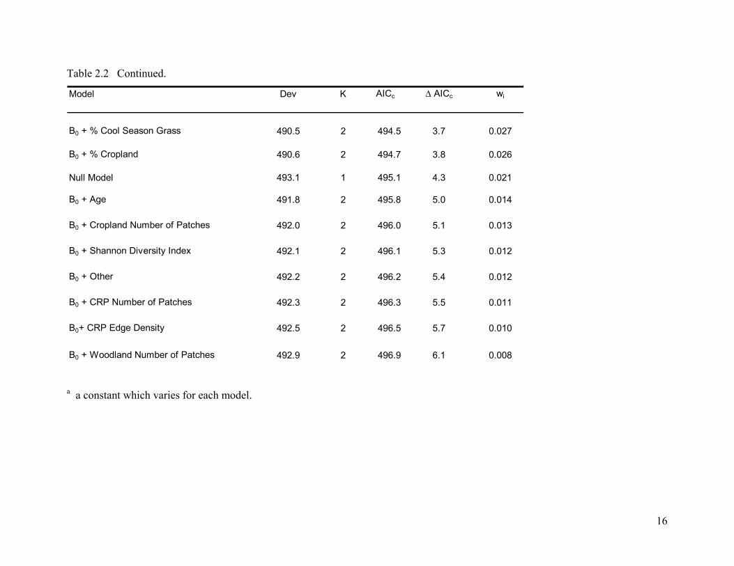
Table 2.2 Continued.


B0 + % Cool Season Grass 490.5 2 494.5 3.7 0.027

B0 + % Cropland 490.6 2 494.7 3.8 0.026

Null Model 493.1 1 495.1 4.3 0.021

B0 + Age 491.8 2 495.8 5.0 0.014

B0 + Cropland Number of Patches 492.0 2 496.0 5.1 0.013

B0 + Shannon Diversity Index 492.1 2 496.1 5.3 0.012

B0 + Other 492.2 2 496.2 5.4 0.012

B0 + CRP Number of Patches 492.3 2 496.3 5.5 0.011

B0+ CRP Edge Density 492.5 2 496.5 5.7 0.010

B0 + Woodland Number of Patches 492.9 2 496.9 6.1 0.008 a a constant which varies for each model.

16

Table 2.3. Model selection for weekly probability of individual survival based on habitat configuration of 500 m buffer around

covey home range during Fall-Spring (1 October to 14 April) for northern bobwhite in southeastern Kansas, USA, 2003 to

2005. Model statistics include the deviance (Dev -2lnℓ), number of parameters (K), Akaike’s Information Criterion (AICc)

corrected for small sample sizes, ∆ AICc, and Akaike weights (wi). Presented are the top 20 models.

Model Dev K AICc ∆AICc wi

B0a + % CRP 488.2 2 492.2 0.0 0.083

B0 + Woodland Mean Patch Size 488.7 2 492.7 0.5 0.063

B0 + % Woodland 489.1 2 493.1 0.9 0.053


B0 +% CRP + % Woodland 487.3 3 493.3 1.1 0.048

B0 + % CRP + % Cropland 487.4 3 493.4 1.2 0.046

B0 + % Other 489.4 2 493.5 1.3 0.044

B0 + Woodland MPS + Cropland MPS 487.5 3 493.6 1.4 0.042

B0 + % CRP + % Native Grass 487.9 3 493.9 1.7 0.035

B0 + % CRP + % Cool Season Grass 488.2 3 494.2 2.0 0.030

continued

17

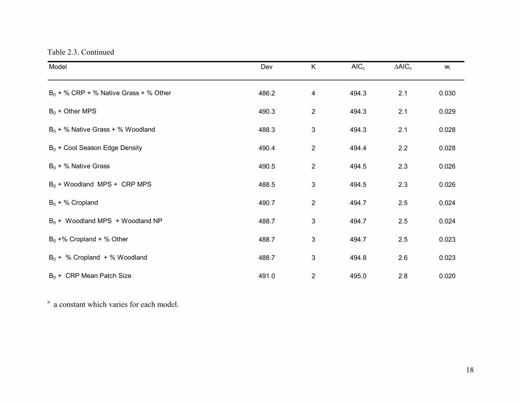
Table 2.3. Continued

Model Dev K AICc ∆AICc wi

B0 + % CRP + % Native Grass + % Other 486.2 4 494.3 2.1 0.030

B0 + Other MPS 490.3 2 494.3 2.1 0.029

B0 + % Native Grass + % Woodland 488.3 3 494.3 2.1 0.028

B0 + Cool Season Edge Density 490.4 2 494.4 2.2 0.028

B0 + % Native Grass 490.5 2 494.5 2.3 0.026

B0 + Woodland MPS + CRP MPS 488.5 3 494.5 2.3 0.026

B0 + % Cropland 490.7 2 494.7 2.5 0.024

B0 + Woodland MPS + Woodland NP 488.7 3 494.7 2.5 0.024

B0 +% Cropland + % Other 488.7 3 494.7 2.5 0.023

B0 + % Cropland + % Woodland 488.7 3 494.8 2.6 0.023

B0 + CRP Mean Patch Size 491.0 2 495.0 2.8 0.020

a a constant which varies for each model.

18

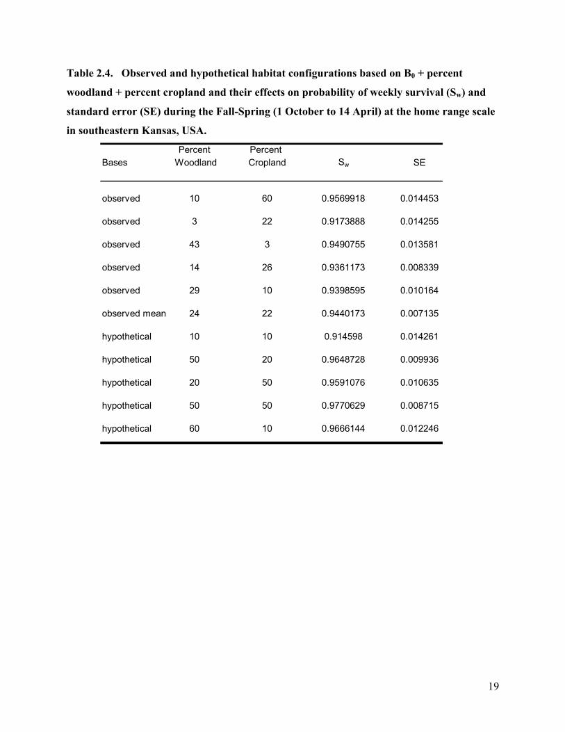
Table 2.4. Observed and hypothetical habitat configurations based on B0 + percent

woodland + percent cropland and their effects on probability of weekly survival (Sw) and

standard error (SE) during the Fall-Spring (1 October to 14 April) at the home range scale

in southeastern Kansas, USA.

Percent Percent Bases Woodland Cropland Sw SE

observed 10 60 0.9569918 0.014453

observed 3 22 0.9173888 0.014255

observed 43 3 0.9490755 0.013581

observed 14 26 0.9361173 0.008339

observed 29 10 0.9398595 0.010164

observed mean 24 22 0.9440173 0.007135

hypothetical 10 10 0.914598 0.014261

hypothetical 50 20 0.9648728 0.009936

hypothetical 20 50 0.9591076 0.010635

hypothetical 50 50 0.9770629 0.008715

hypothetical 60 10 0.9666144 0.012246

19

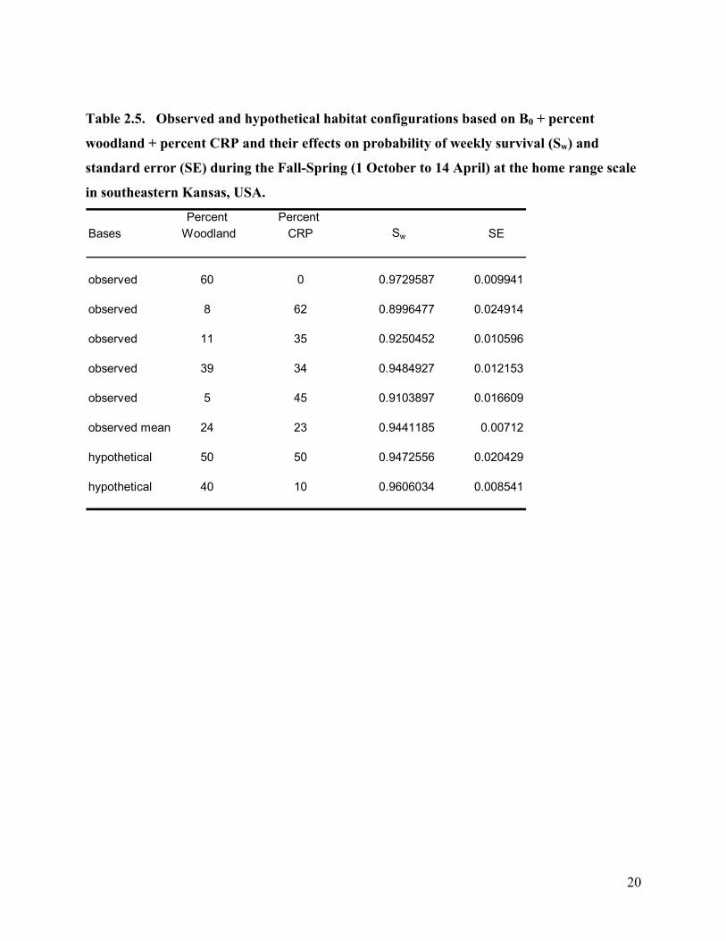
Table 2.5. Observed and hypothetical habitat configurations based on B0 + percent

woodland + percent CRP and their effects on probability of weekly survival (Sw) and

standard error (SE) during the Fall-Spring (1 October to 14 April) at the home range scale

in southeastern Kansas, USA.

Percent Percent Bases Woodland CRP Sw SE

observed 60 0 0.9729587 0.009941

observed 8 62 0.8996477 0.024914

observed 11 35 0.9250452 0.010596

observed 39 34 0.9484927 0.012153

observed 5 45 0.9103897 0.016609

observed mean 24 23 0.9441185 0.00712

hypothetical 50 50 0.9472556 0.020429

hypothetical 40 10 0.9606034 0.008541

20

Table 2.6. Model selection for comparison of burned CRP versus nonburned CRP

individual weekly probability of surviving for northern bobwhite in southeastern Kansas,

USA, 2003 to 2005 during Fall-Spring (1 October to 14 April). Model statistics include the

deviance (Dev -2lnℓ), number of parameters (K), Akaike’s Information Criterion (AICc)

corrected for small sample sizes, ∆ AICc, and Akaike weights (wi).

Model Dev K AICc ∆ AICc Wi

Burn vs Not Burned 217.0 2 221.0744 0.0 0.767

Null Model 221.4 1 223.4533 2.4 0.233

21

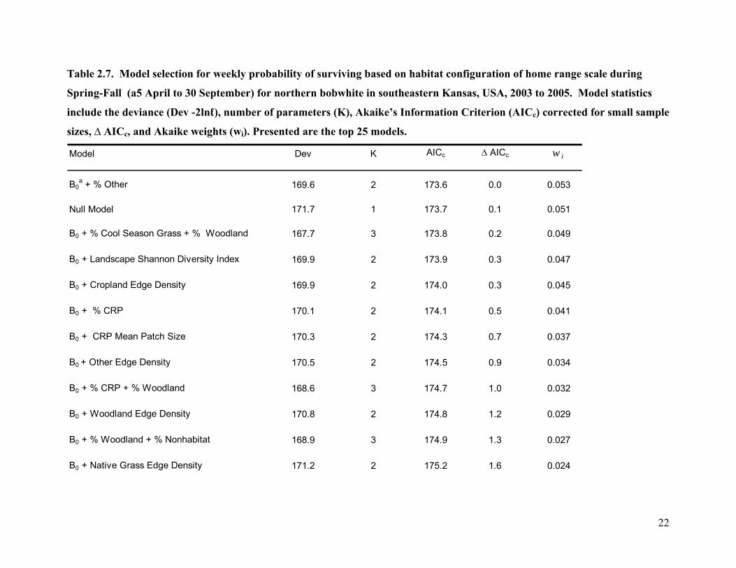
Table 2.7. Model selection for weekly probability of surviving based on habitat configuration of home range scale during

Spring-Fall (a5 April to 30 September) for northern bobwhite in southeastern Kansas, USA, 2003 to 2005. Model statistics

include the deviance (Dev -2lnℓ), number of parameters (K), Akaike’s Information Criterion (AICc) corrected for small sample

sizes, ∆ AICc, and Akaike weights (wi). Presented are the top 25 models.

Model Dev K AICc ∆ AICc w i

B0a + % Other 169.6 2 173.6 0.0 0.053

Null Model 171.7 1 173.7 0.1 0.051

B0 + % Cool Season Grass + % Woodland 167.7 3 173.8 0.2 0.049

B0 + Landscape Shannon Diversity Index 169.9 2 173.9 0.3 0.047


B0 + % CRP 170.1 2 174.1 0.5 0.041


B0 + Other Edge Density 170.5 2 174.5 0.9 0.034

B0 + % CRP + % Woodland 168.6 3 174.7 1.0 0.032

B0 + Woodland Edge Density 170.8 2 174.8 1.2 0.029

B0 + % Woodland + % Nonhabitat 168.9 3 174.9 1.3 0.027

B0 + Native Grass Edge Density 171.2 2 175.2 1.6 0.024

22

Table 2.7. Continued.

Model Dev K AICc ∆ AICc w i

B0 + % Woodland 171.2 2 175.2 1.6 0.024


B0 + Landscape Edge Density 171.2 2 175.2 1.6 0.024

B0 + % Cool Season Grass 171.3 2 175.3 1.7 0.023

B0 + % Cropland 171.3 2 175.3 1.7 0.023

B0+ % Native Grass 171.3 2 175.3 1.7 0.023

B0 + Native Grass Mean Patch Size 171.3 2 175.3 1.7 0.023

B0 + % CRP = % Native Grass 169.3 3 175.4 1.7 0.022

B0 + Sex 171.5 2 175.5 1.9 0.021

B0 + Woodland Number of Patches 171.5 2 175.5 1.9 0.020

B0 + % Cool Season Grass + % Other 169.5 3 175.5 1.9 0.020

B0 + Cropland Mean Patch Size 171.6 2 175.6 2.0 0.020

B0 + Cropland Edge Density 171.6 2 175.6 2.0 0.019 a a constant which varies for each model.

23

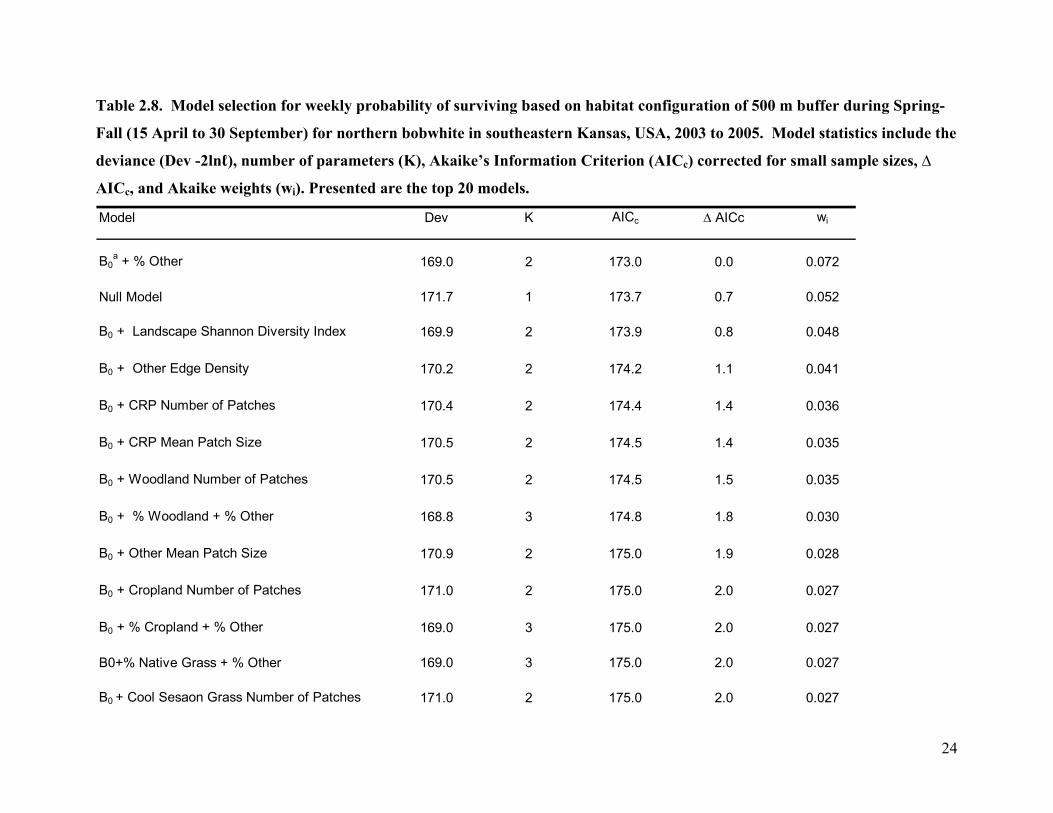
Table 2.8. Model selection for weekly probability of surviving based on habitat configuration of 500 m buffer during Spring-

Fall (15 April to 30 September) for northern bobwhite in southeastern Kansas, USA, 2003 to 2005. Model statistics include the

deviance (Dev -2lnℓ), number of parameters (K), Akaike’s Information Criterion (AICc) corrected for small sample sizes, ∆

AICc, and Akaike weights (wi). Presented are the top 20 models.


B0a + % Other 169.0 2 173.0 0.0 0.072

Null Model 171.7 1 173.7 0.7 0.052

B0 + Landscape Shannon Diversity Index 169.9 2 173.9 0.8 0.048

B0 + Other Edge Density 170.2 2 174.2 1.1 0.041



B0 + Woodland Number of Patches 170.5 2 174.5 1.5 0.035

B0 + % Woodland + % Other 168.8 3 174.8 1.8 0.030

B0 + Other Mean Patch Size 170.9 2 175.0 1.9 0.028

B0 + Cropland Number of Patches 171.0 2 175.0 2.0 0.027

B0 + % Cropland + % Other 169.0 3 175.0 2.0 0.027

B0+% Native Grass + % Other 169.0 3 175.0 2.0 0.027

B0 + Cool Sesaon Grass Number of Patches 171.0 2 175.0 2.0 0.027

24



B0 + % Cool Season Grass + % Other 169.0 3 175.1 2.0 0.026

B0 + Native Grass Number of Patches 171.2 2 175.2 2.2 0.024

B0 + Cool Season Grass Edge Density 171.2 2 175.2 2.2 0.024

B0 + Landscape Mean Patch Size 171.2 2 175.2 2.2 0.024

B0 + Cropland Mean Patch Size 171.3 2 175.4 2.3 0.023

B0 + Other Number of Patches 171.4 2 175.4 2.3 0.022

B0 + Cool Season Grass Mean Patch Size 171.4 2 175.4 2.4 0.022

a a constant which varies for each model.

25

Figure 2.1. Weekly survival probabilities for southeastern Kansas, USA, with upper (---)

and lower (···) confidence intervals for northern bobwhite based on most parsimonious

model, B0 + percent CRP, during the Fall-Spring (1 October to 30 September) at the 500 m

buffer scale.

26

27

Figure 2.2. Weekly survival probabilities for southeastern Kansas, USA, with upper (---)

and lower (···) confidence interval for northern bobwhite based on second most

parsimonious model, B0 + Woodland Mean Patch Size, during the Fall-Spring (1 October

to 14 April) at the 500 m buffer scale.

28

29

CHAPTER 3 - Distance – Based Habitat Associations of Northern

Bobwhite in Southeastern Kansas

Abstract The northern bobwhite (Colinus virginianus) has been studied extensively over the last 30+

years. However, throughout much of its range bobwhite carrying capacity has been reduced or

eliminated. The reduction in numbers has been attributed to changes in land use. Ironically very

little research has been done to determine the overall affects of land use changes on bobwhite

movement and habitat associations at the landscape scale. I used the Euclidean distance method

to characterize land cover and land use associations of bobwhite during Spring-Fall (15 April to

30 September 0) and Fall-Spring (1 October to 14 April). The first classification level included

broad land cover classes such as cool season grass or native warm season grass, while the second

more refined classification included land uses such as cool season pasture and burned

Conservation Reserve Program (CRP). The Euclidean distance method uses animal

location/random location distance ratios to determine if distances to the various habitats differ

from random. Habitat selection was found to occur during the Spring-Fall (Wilkes λ = 0.04, F 6,36

= 143.682, P < 0.001) and Fall-Spring (Wilkes λ = 0.056, F 6, 29 = 81.99, P < 0.001). Ranking of

the Spring-Fall habitats showed that bobwhite were associated withlocations in close proximity

to cool season grasses over all other habitats. During the Fall-Spring covey location were

randomly associated with cool season grasses (t34 = -1.002, P =0.323). Habitat rankings showed

that covey’s preferred locations in close proximity to woody cover. Bobwhite showed habitat

selection based on land use for Spring-Fall (Wilkes λ = 0.006, F 16, 26 = 284.483, P < 0.001) and

Fall-Spring (Wilkes λ = 0.004, F 16, 19 = 276.037, P < 0.001). During the Spring-Fall, bobwhites

were associated with locations in close proximity to cool season grass pastures and roads equally

over all other habitats. During the Fall-Spring coveys preferred locations in close proximity to

roads and CRP lands. Bobwhite used a variety of different land covers types within the

landscape and its usage varied between seasons. Cool season grasses may have a bigger impact

on bobwhites during the Fall-Spring when the short vegetation results in increased fragmentation

of the landscape forcing birds into small patches of winter cover.

30

Introduction The northern bobwhite (Colinus virginianus) is one of the most studied game birds in

North America. Even with the amount of research that has been done in many parts of the range

over the last 30+ years, most populations continue to decline or remain low. This decline and

lack of rebound in bobwhite populations has often been attributed to changes in land use,

particularly changes in farming practices (Brennan 1991, Church and Taylor 1992, Brady et

al.1993, Peterson et al. 2002). Researchers have theorized that the wide spread shift to clean

farming has made the landscape less favorable to bobwhite through fragmentation and reduction

of important idle areas.

The widespread use of cool season grasses such as tall fescue (Schedomorus phoenix) has

been hypothesized to have contributed to the decline of bobwhite. Yet very little research has

been done in this area. No research has been conducted on the effects of cool season grasses like

fescue on the habitat associations during the life cycle of bobwhite. Much of the limited research

on fescue was conducted in undisturbed areas (Burger et al. 1990, Barnes et al 1995). One of the

reasons that fescue has been thought of as poor habitat for bobwhite is its limited diversity and

the lack of bare ground in stands of fescue (Barnes et al. 1995). Kuvlesky et al. (2002) indicated

that more research was needed in order to quantify the specific effects of fescue and other cool

season grasses on bobwhite throughout their range.

A number of studies have been conducted on the habitat associations of bobwhite in

various parts of the range, but usually only during one period, either Fall-Spring or Spring-Fall.

For instance Dixon et al. (1996) studied the habitat associations of bobwhite in North Carolina

during the Fall-Spring. Taylor et al. (1999) studied the habitat associations of bobwhite on 2

study areas during the Spring-Fall in the Flint Hills of Kansas. While Williams et al. (2000)

studied bobwhites in the same areas as Taylor et al. (1999) during different years and different

seasons (Fall-Spring). The problem with only studying habitat usage during one particular

season is that the quality of the habitat may change between seasons resulting in a particular

habitat being of less value at different times of the year. Changes in plant structure can result in

increased fragmentation of the landscape during different periods reducing the movement of

bobwhite.

Past studies on habitat use and availability often grouped habitats into generalized

categories that resulted in a particular habitat appearing to be less important than it should be.

31

Williams et al. (2000) grouped CRP, grassy waterway and roadsides into one categoery “idle

grassland”. Taylor et al. (1999) grouped woodland and wetlands into one category “other”. Few

studies of habitat associations use the same habitat categories and even less use more than 5

categories. These generalizations can also make it more difficult to assess the specific habitat

needs of bobwhite within the landscape.

Edge has been hypothesized to be an important habitat component for bobwhites

(Stoddard 1931, Rosene 1984). However, very little information is available on the preference of

bobwhite for various edge types or what constitutes acceptable edge. Roseberry and Sudkamp

(1998) found that Illinois bobwhites were associated with patchy landscapes that contained

moderate amounts of row crops, grassland, and abundant woody edge.

My objectives for this study were to determine 1) the effects of landscape configuration

in a fescue dominated agricultural system on bobwhite locations during the year using Euclidean

distances; and 2) the effect of specific land cover types on habitat associations of bobwhite.

Study Area The study area is a 64.75 km2 area located in the southwestern corner of Bourbon County,

Kansas, 3.2 km south of Uniontown. The area is also a demonstration area for the Quail

Initiative sponsored by Kansas Department of Wildlife and Parks and other cooperators. It

consists of large fescue pastures and hayfields intermixed with native warm season grass

pastures and hayfields. Large tracts of cropland are located within the floodplains of streams and

creeks. Smaller tracts of cropland are scattered throughout the upland. There are narrow

riparian forests interconnected with small woodlots and linear wooded fencerows throughout the

area. Many of the fencerows consist of Osage Orange (Maclura pomifera) >50 years of age.

Conservation Reserve Program (CRP) lands are scattered throughout the uplands and in small

patches in the floodplains of streams and creeks. CRP consist of a mix of native warm season

grasses including big bluestem (Adropogon gerardii), yellow Indiangrass (Sorghastrum nutans),

and Switchgrass (Panicum virgatum).

The land cover of the study area changed very little over the course of the study. Most

changes occurred between CRP and Cropland (Table 3.1). Woodland patch size on the study area

ranged from 0.4 to 332.2 ha. Cropland patch size in the study area ranged from 0.1 ha to 83.5 ha.

Cool-season grass patch size ranged from 0.3 to 282.2 ha. Native warm-season grass patches

32

ranged from 0.1 to 128.9 ha. CRP tract sizes in the study area were relatively small and isolated

ranging in size from 0.5 ha to 58 ha.

Methods Bobwhites were trapped from January through March and October through December in

2003 and 2004 using baited funnel traps on eight 0.64 km2 areas. All captured birds were sexed,

aged, weighed, and banded. Three to 6 random individuals within each covey weighing >150 g

were fitted with a necklace transmitter weighing <5 g. In late March all individuals caught were

equipped with radio transmitters to examine dispersal patterns. Bobwhite were located 3 to 7

times/week until mortality, loss of contact (radio failure or long distance movement), or end of

study. All bobwhite were released immediately after processing at the capture location.

Bobwhites with radio transmitters were located using a combination of 3-element yagi

antennas and 4-element null peak vehicle antennas. Homing and short distance triangulation (<

200 m) were conducted with hand held antennas. UTM gridded aerial photos were used to record

location of bobwhite when homing and short distance triangulation was used. When bobwhite

were flushed, a Garmin Legend Global Positioning System (GPS) was used to record the

location within 5 m. Vehicle telemetry consisted of 2 to 3 bearings taken rapidly in order to

triangulate the radio-equipped bobwhite’s location. A GPS was used to record the base stations

for vehicle triangulation. I used the program LOAS (Ecological Software Solutions, Urnsach,

Switzerland) to estimate locations of radio collared bobwhite based on triangulation data.

Mortalities were determined by signal strength and fluctuation. When mortality was

suspected I homed in on the transmitter in order to find the bobwhite carcass and transmitter to

determine the cause of death. The cause was determined based on the bobwhite remains and

marks on the transmitter. Mortalities were classified as avian, mammalian, and unknown. For

each mortality location I also recovered the location to within <5 m using a Garmin GPS. I also

recorded the habitat type of each mortality site.

Land cover on the study area was on-screen digitized in ArcView 3.3 (Environmental

Systems Research Institute, Inc., Redlands, CA). I used 2002 Digital Orthophoto Quarter Quads

(DOQQ) as well as 2003, 2004, and 2005 National Agricultural Inventory Program (NAIP)

digital color aerial photos as base maps for land cover analysis. The DOQQs and NAIP digital

color aerial photos were obtained from Kansas Data Access and Support Center (DASC). Land

33

cover was classified for 2003, 2004, and 2005. Land cover classifications were other (farmstead,

urban, rock quarry, roads, and farm ponds), cool season grassland (cool season hayfield, cool

season pasture, cool season waterway, and idleland), native grassland (native hayfield, native

rangeland, and native waterway), woodland (fencerows and woodlots), and CRP (new CRP,

burned CRP, and established general sign-up CRP). New CRP was general sign-up CRP and

continuous sign-up CRP that was < 2 years of age. Burned CRP was those areas burned during

March and April through the first growing season and up until the Mid April of the following

year. Land use categories were farmstead, road, farm pond, cool season hayfield, cool season

pasture, cool season waterway, idleland, native hayfield, native rangeland, native waterway, new

CRP, burned CRP, and established general sign-up CRP. All areas were ground truthed each

year in order to obtain an accurate map.

Habitat Association Analysis

I used the Euclidean distance approach (Conner and Plowman 2001, Conner et al. 2003)

of analyzing habitat use during Fall-Spring and Spring-Fall because of its advantages over other

methods. Conner et al. (2003) found that the Euclidean distance approach identified edges as

important habitat features and was not affected by location error. Bingham and Brennan (2004)

found that this method did not inflate Type I error like other methods. The Euclidean distance

method uses a ratio of use versus expected distance to habitat. If habitat use is nonrandom then

the observed/random ratio should equal 1.0 for each habitat type. If the habitat is associated

disproportionately the ratio can be used to determine which habitat is associated more or less

with the animal. If the observed/random ratio is low (<1.0) then the animal is associated more

with the habitat than expected. If the observed/random ratio is high (>1.0) then the habitat is

associated less with the animal than expected

I conducted home range analysis for Fall-Spring (1 October to 14 April) and for Spring-

Fall (15 April through 30 September). I used the Animal Movements 2.04 extension (Hooge and

Eichenlaub 2000) for ArcView to remove 5% of the outlier locations before conducting home

range analysis. I used the Animal Movements extension to calculate the 95% fixed kernel home

range for each covey (Fall-Spring) and individual (Spring-Fall). I used ArcView 3.3 to buffer

each home range at 1000 m. I then used the Animal Movement Extension to generate 30

uniformly random points within each buffer for each home range. Each habitat for 2003, 2004,

34

and 2005 was separated into different layers, and the ArcView extension Nearest Neighbor

(Weigel 2004) was used to get the distance from each random location and bobwhite location to

each habitat type for each year. The Nearest Neighbor analysis was done at both the level 1 and

level 2 land cover classification levels. For the land cover and land use classifications I did not

use urban and rock quarry classes in the analysis due to their lack of importance for bobwhite

and limited occurrence in the landscape.

I calculated rj which was the average distance to each land cover type for random

locations for each animal or covey depending on the season. I then calculated ui which was the

average distance to each habitat for each bobwhite or covey. I created di which was a vector of

ratios for each bobwhite or covey by dividing ui by rj. The expected value of each element in the

di is 1.0 under the null hypothesis of no selection. I used MANOVA to test for significance of di

for sex and year. The mean of the di was ρ and MANOVA was used to determine if ρ differed

from a vector of ones. I used the Wilkes lambda test statistic to indicate non-random resource

selection (Conner and Plowman 2001). To determine which habitat types were used

disproportionately I tested each element of ρ for each habitat type against 1 using a paired t-test.

If a statistically significant element of ρ was >1 then the animal was associated less with the

habitat. If a statistically significant element of ρ was <1 then animal was associated more with

the habitat. I also tested whether a particular habitat type was associated more over the other

habitat types by using a paired t-test. The pair-wise test provided a habitat ranking matrix

similar to the compositional analysis approach of Aebischer et al. (1993). All analyses were

conducted for land cover and land use. All statistical analyses were conducted in SPSS 12.0

(SPSS Inc., Chicago, IL).

Results A total of 42 individuals (17 females and 24 males) during Spring-Fall and 35 coveys

during Fall-Spring were used for the Euclidean-distance analysis. There was no significant

difference in habitat association by sex during the Spring-Fall (Wilkes λ = 0.885, F 6, 35 = 0.756,

P = 0.609). Therefore for Fall-Spring and Spring-Fall I pooled the data by sex. There was no

detectable difference in habitat association between years for Fall-Spring (Wilkes λ = 0.523, F12,

54 = 1.724, P= 0.087). However there was a significant difference in habitat association between

years for the Spring-Fall (Wilkes λ = 0.516, F12, 68 = 2.219, P = 0.02). I also pooled the data by

35

year for Fall-Spring and Spring-Fall. Even though the MANOVA showed a significant

difference in habitat association for the Spring-Fall period the small sample sizes in 2004 and

2005 may have resulted in an inflated difference.

Land Cover Analysis

Analysis of habitat associations using Euclidean distance for the Spring-Fall indicated

that habitat selection was occurring (Wilkes λ = 0.04, F 6,36 = 143.682, P < 0.001). During the

Spring-Fall bobwhite were found significantly closer than expected to woody cover (t41=-4.065,

P <0.001), other (t41 = -6.336, P <0.001), cool season grassland (t41= -8.872, P <0.001), and CRP

(t41= -8.872, P <0.001). Bobwhite locations did not show significant proximity to native

grassland (t41= -0.707, P = 0.483) and cropland (t41= 0.848, P = 0.401). Based on pair-wise

comparisons bobwhite locations were associated more with cool season grasses over all other

habitats during the Spring-Fall period (Table 3.2).

When I examined the habitat associations for the Fall-Spring using Euclidean distance I

found that habitat selection was occurring (Wilkes λ = 0.056, F 6, 29 = 81.99, P < 0.001). During

this period coveys were found to be significantly closer than expected to woody cover (t34 = -

11.563, P <0.001), other (t34 = -3.630, P = 0.001), native grassland (t34 = -2.658, P = 0.012),

CRP (t34 = -5.642, P < 0.001), and cropland (t34 = -2.915, P = 0.006). Covey locations were not

associated with cool season grasses (t34 = -1.002, P = 0.323) during Fall-Spring. Based on the

pair-wise comparisons, covey where associated more with locations closer to woody cover over

all other habitats during the Fall-Spring (Table 3.3).

Land Use Analysis

Bobwhite during the Spring-Fall showed habitat selection for land uses (Wilkes λ =

0.006, F 16, 26 = 284.483, P < 0.001). They were found to be significantly closer than expected to

burned CRP (t41 = -4.878, P <0.001), CRP (t41 = -3.119, P = 0.003), woody fencerow (t41 = -

2.910, P = 0.006 ), cool season pasture (t41 = -4.091, P <0.001), cool season waterway (t41 = -

2.224, P = 0.32), native grass hayland (t41 = -2.121, P = 0.40), native grass waterway (t41 = -

3.441, P = 0.001), new CRP (t41 = -3.526, P = 0.001), ponds (t41 = -3.667, P = 0.001), and

roads (t41 = -4.772, P <0.001). Bobwhite did not show a significant proximity to woodlots (t41 = -

1.884, P = 0.067), cropland (t41 = 0.803, P = 0.427), farmsteads (t41 = -0.424, P = 0.674), cool

season hayland (t41 = -0.377, P = 0.708), idleland (t41 = 0.449, P = 0.656), and native grass

36

pasture (t41 = -0.684, P = 0.498). During the Spring-Fall, bobwhites were associated with

locations in close proximity to cool season grass pastures and roads more than other habitats

(Table 3.4).

Coveys during the Fall-Spring selectively used land use classes (Wilkes λ = 0.004, F 16, 19

= 276.037, P < 0.001). Coveys were found to be significantly closer to woodlots (t34 = -2.813, P

= 0.008), burned CRP (t34 = -2.588, P =0.14), cropland (t34 =-2.602, P = 0.014), CRP (t34 = -

3.438, P = 0.002), woody fencerow (t34 = -2.322, P = 0.26), idleland (t34 = -3.031, P = 0.005),

native grass pasture (t34 = -2.309, P = 0.27), native grass waterway (t34 = -3.346, P = 0.002), new

CRP (t34 = -3.431, P = 0.002), roads (t34 = -5.067, P < 0.001). Coveys were significantly further

from cool season pastures than expected (t34 = 2.491, P = 0.018). Coveys did not show a

significant proximity to farmsteads (t34 = 0.348, P = 0.730), cool season hayland (t34 = -0.111, P

= 0.912), cool season waterway (t34 = -1.284, P = 0.208), native grass hayland (t34 = -1.351, P =

0.186), and ponds (t34 = -1.772, P = 0.085). Based on pair-wise comparisons, coveys were

associated more with locations that were in close proximity to roads and CRP (Table 3.5).

Discussion Habitat associations of bobwhite varied between Spring-Fall and Fall-Spring within the

context of the landscape based on land cover and land use classification schemes. This variability

was due to changes in vegetation structure as well as biological needs of bobwhite throughout

their life cycle. Conner et al. (2003) distance analysis showed greater use of “edge” than

expected. This use of edge was only associated with some of the habitats. In Kansas, bobwhite

during the Spring-Fall preferred edges of woody cover, other, cool-season grass, and CRP.

During the Fall-Spring bobwhite preferred edge of woody cover, other, native grassland, CRP,

and cropland.

There was a distinct shift in proximity of bobwhite locations between seasons. Bobwhite

show an avoidance of cool season grasses during the Fall-Spring, but a preference for this habitat

during the Spring-Fall. When examining the land use, cool-season pasture is preferred during the

Spring-Fall and avoided during Fall-Spring. This change in proximity was probably due to

changes in vegetation characteristics between the two periods as well as changes in the biological

needs of bobwhite. During the Fall-Spring, continuous grazing of cool season grasses and

changes in plant growth resulted in extremely short vegetation. The change in vegetation height

37

becomes most pronounced from December through early April in Kansas. This short vegetation

does not provide thermal cover or protection from predators. In fact coveys that form in late

September and October in areas with cool season grasses often disappear by late November

either due to increased predation or movement to more suitable habitats.

The reduction of vegetation height also can have a significant effect on habitat

connectivity between suitable habitat patches. Large areas of cool season grasses can reduce

movement of bobwhite between wintering habitat and thus reduce overall survival of individuals.

It can also result in concentration of bobwhite into small patches. Williams et al. (2003) found

that quail had an optimal group size of 11 individuals, as group size increased survival decreased

for individuals, movement increased, and individual mass decreased. Small groups from 1 to 7

individuals also had lower group persistence, individual survival, and increased movement

(Williams et al. 2003).

Starting in late April cool season grasses begin to regrow and reach a point at which they

are able to provide some cover for bobwhite. In Kansas this occurs during mid-May when coveys

begin to break up and individuals begin to disperse throughout the landscape. The heavy grazing

that cool grasses received in the study area often resulted in a mix of short grass and tall thick

patches during the summer with a variety of short annual weeds mixed in. However, Barnes et al.

(1995) felt that tall fescue was not good bobwhite habitat because it lacked proper vegetation

structure, floristic composition, and sufficient food. Sole (1995) found that bobwhites and

eastern cottontail rabbits (Sylviagus floridanus) did not use a fescue field but did use a field

converted from fescue to native warm-season grasses.

Woody cover had a higher habitat ranking in the Fall-Spring than in the Spring-Fall.

There is also a difference at the second land cover classification level where woody fencerows

had a higher ranking than woodland during the Spring-Fall than during the Fall-Spring. Woody

fencerows were linear areas throughout the study area that composed of 70-100 year old trees or

a mix of shrubs, grasses and forbs. Woodlands in the study area were found along riparian areas

and as large patches of trees in cool-season grass pastures.

Williams et al. (2000) found that woody cover (treelines and wooded drainage ways) was

the primary escape cover for bobwhite during the winter in east-central Kansas. Wiseman and

Lewis (1981) found that woody cover (tall shrubs, short shrubs, and woodland) were important

habitats year round for bobwhite in the tallgrass prairie of Oklahoma. Woody cover provided

38

feeding, resting, and escape cover for quail throughout the year (Wiseman and Lewis 1981). The

change from woodland to woody fencerows in the Spring-Fall on the study area was most likely

due to avoidance of possible predator sources in the riparian areas and movement away from

more intensive agricultural areas to areas containing more grasslands. Taylor and Burger (2000)

found that bobwhite during the breeding season in Mississippi allocated time and resources more

to woody areas and old fields that were burned and disked.

Woody fencerows were often associated with cool season grass pastures. Many

fencerows associated with cool season grass pastures were grazed and had reduced shrub cover

and forbs compared to fencerows associated with road edges and CRP which were not as

disturbed. Bobwhite preference for locations in close proximity to woodlands during the Fall-

Spring was most likely due to the association of woodlands to CRP fields in the study area.

Woodland edge probably provided more food, resting, and escape cover during the Fall-spring

due to the larger width and diversity of shrubs and forbs found growing around them.

Bobwhites had a higher preference for CRP edge during the Fall-Spring than during the

Spring-Fall. Williams et al. (2000) found that bobwhite showed a preference for idleland which

included CRP, grassy waterways, and roadsides during the winter. Taylor et al. (1999) also

found that idleland which consisted of 62% CRP was a preferred habitat in Kansas during the

breeding season in both cropland and rangeland areas. Very little other information on use of

CRP is available. This lack of research has resulted in limited changes to CRP thus resulting in

the limited benefits of CRP to bobwhite. During the Fall-Spring CRP edge was preferred over

new CRP and burned CRP. New CRP edge was preferred to burned CRP edge, possibly because

burned areas contained fewer forbs than CRP and new CRP due to the disturbance. However

during the Spring-Fall burned CRP edge was preferred over CRP edge and new CRP edge, and

CRP edge was preferred over new CRP. Burned CRP may have been preferred in the breeding

season due to increased bare ground and shorter vegetation which made the areas more favorable

for movement and feeding by broods.

During both Spring-Fall and Fall-Spring bobwhite were found to favor road edges. In

fact, during Fall-Spring bobwhite preference of road edges over all other land cover classes.

Road edges during Spring-Fall were associated with cool-season grass pasture. Roads may act as

dusting and feeding areas. Also in many instances roadsides contained fencerows or scattered

39

trees that could provide escape cover for bobwhite throughout the year. Road edges were often

mown, but unlike pastures fencerows often had fewer disturbances.

Management Implications Managers need to focus on increasing habitat connectivity within fescue dominated

landscapes. This is particularly important during the Fall-Spring when grazing and dormancy of

cool season grasses reduces plant height and isolates patches of winter cover. Ideal connectivity

can be created through increasing and protecting woody cover within the landscape. In pastured

areas woody fencerows and riparian zones need to be protected from grazing. Woodlots which

are wider than fencerows provide ideal wintering cover when in close proximity to idle

grasslands such as CRP. Increasing the width of existing fencerows could increase usage by

bobwhite during the Fall-Spring. Also converting portions of cool-season pastures along

fencerows to native warm grass buffers may allow for increased connectivity and provide more

areas for coveys to survive during the winter as well as providing secure nesting cover.

Management of CRP can also have a great impact on use by bobwhite. Burning CRP can

provide needed brood rearing habitat during the breeding season, but lacks the essential

microhabitat and forbs needed to support coveys during the Fall-Spring. Managers should be

encouraged to use patch burning to increase diversity of plants within CRP. The bobwhite is a

grassland/woodland transitional species needing a diversity of forbs, grasses, and woody cover to

survive. Under current planting recommendations and management, CRP lacks these

components. More emphasis needs to be placed on creating woody cover in and around CRP to

mimic a late successional old field community.

40

Table 3.1. Percentage of level 2 land use classes from 2003 to 2005 for the study in

southeastern Kansas, USA.

2003 2004 2005

Burned CRPa 0.6 0.1 2.5

CRPa 3.2 3.8 1.4

Cropland 21.1 19.9 19.9

Farm Pond 0.5 0.5 0.5

Farmstead 1.0 1.0 1.0

Idleland 1.2 1.2 1.2

Native Grass Hayfield 1.6 1.6 1.6

Native Grass Pasture 4.3 4.3 4.3

Native Grass Waterway 0.1 0.1 0.1

New CRPa 0.3 1.4 1.4

Road 0.9 0.9 0.9

Woodland 20.6 20.6 20.6

Woody Fencerow 1.6 1.6 1.6

Cool Season Grass Hayfield

Cool Season Grass Pasture

Cool Season Grass Waterway 0.9 0.9 0.9

5.8 5.8 5.8

36.3 36.3 36.3

a Conservation Reserve Program.

41

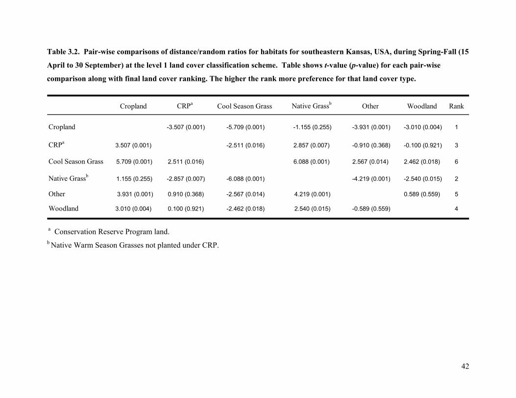
Table 3.2. Pair-wise comparisons of distance/random ratios for habitats for southeastern Kansas, USA, during Spring-Fall (15

April to 30 September) at the level 1 land cover classification scheme. Table shows t-value (p-value) for each pair-wise

comparison along with final land cover ranking. The higher the rank more preference for that land cover type.

Cropland CRPa Cool Season Grass Native Grassb Other Woodland Rank

Cropland -3.507 (0.001) -5.709 (0.001) -1.155 (0.255) -3.931 (0.001) -3.010 (0.004) 1

CRPa 3.507 (0.001) -2.511 (0.016) 2.857 (0.007) -0.910 (0.368) -0.100 (0.921) 3

Cool Season Grass 5.709 (0.001) 2.511 (0.016) 6.088 (0.001) 2.567 (0.014) 2.462 (0.018) 6

Native Grassb 1.155 (0.255) -2.857 (0.007) -6.088 (0.001) -4.219 (0.001) -2.540 (0.015) 2

Other 3.931 (0.001) 0.910 (0.368) -2.567 (0.014) 4.219 (0.001) 0.589 (0.559) 5

Woodland 3.010 (0.004) 0.100 (0.921) -2.462 (0.018) 2.540 (0.015) -0.589 (0.559) 4

a Conservation Reserve Program land. b Native Warm Season Grasses not planted under CRP.

42

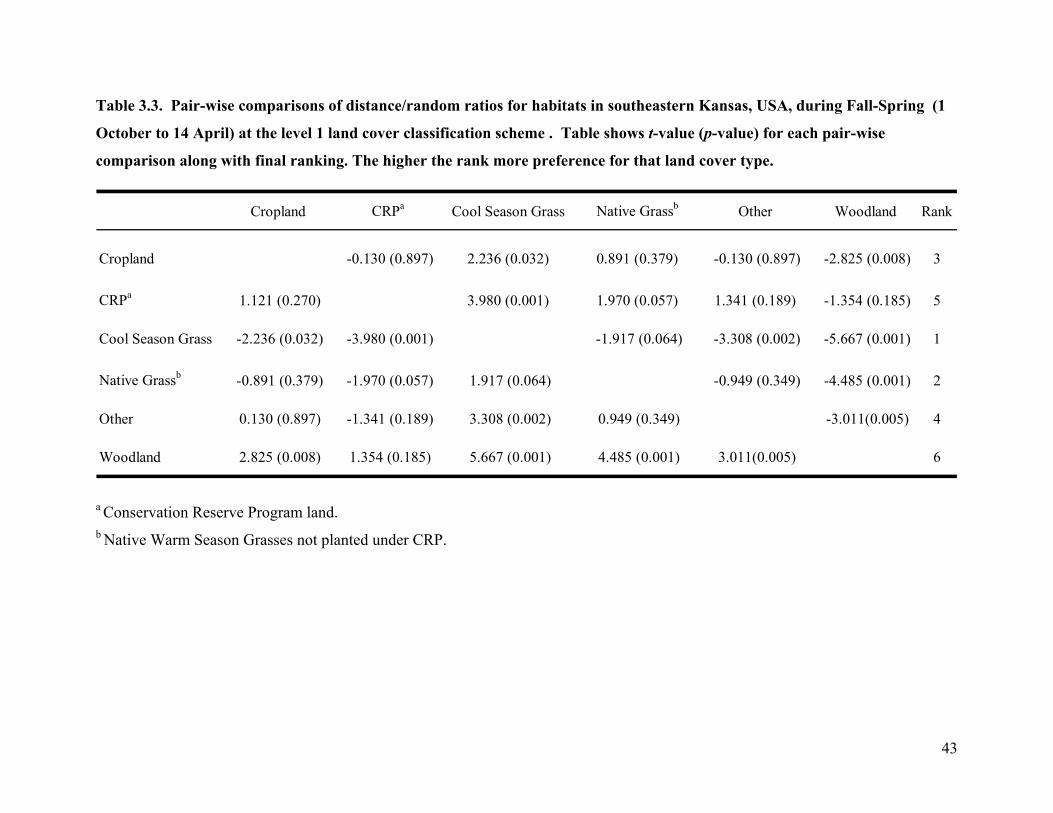
Table 3.3. Pair-wise comparisons of distance/random ratios for habitats in southeastern Kansas, USA, during Fall-Spring (1

October to 14 April) at the level 1 land cover classification scheme . Table shows t-value (p-value) for each pair-wise

comparison along with final ranking. The higher the rank more preference for that land cover type.

Cropland CRPa Cool Season Grass Native Grassb Other Woodland Rank

Cropland -0.130 (0.897) 2.236 (0.032) 0.891 (0.379) -0.130 (0.897) -2.825 (0.008) 3

CRPa 1.121 (0.270) 3.980 (0.001) 1.970 (0.057) 1.341 (0.189) -1.354 (0.185) 5

Cool Season Grass -2.236 (0.032) -3.980 (0.001) -1.917 (0.064) -3.308 (0.002) -5.667 (0.001) 1

Native Grassb -0.891 (0.379) -1.970 (0.057) 1.917 (0.064) -0.949 (0.349) -4.485 (0.001) 2

Other 0.130 (0.897) -1.341 (0.189) 3.308 (0.002) 0.949 (0.349) -3.011(0.005) 4

Woodland 2.825 (0.008) 1.354 (0.185) 5.667 (0.001) 4.485 (0.001) 3.011(0.005) 6

a Conservation Reserve Program land. b Native Warm Season Grasses not planted under CRP.

43

Table 3.4. Simplified ranking matrices based on pair-wise comparisons of distance/random ratios for each land use class

during Spring-Fall (15 April to 30 September). Each element in the matrix was replaced by its sign; a triple sign represents

significant difference at the P < 0.05. A + represents a positive association and a – represents a negative association. The

higher the rank more preference for that land use type. B

CR

Pa

Cro

plan

d

CR

Pb

Farm

c

Fenc

ed

CSG

He

CSG

Pf

CSG

Wg

Idle

land

NG

H h

NG

P i

NG

W j

New

CR

P

Pond

Roa

d

Woo

dlot

Rank

BCRPa +++ + +++ + +++ − + +++ +++ +++ +++ +++ + − + 13

Cropland − − − − − − − − − − − − − − − − − − − − − − − − − − − − − − − 1

CRPb − +++ + − + − + +++ + + + + − − − 9

Farmc − − − + − − + − − − − + − + − − − − − − − − − 3

Fenced − +++ + + + − + +++ + +++ + + + − + 12

CSGHe − − − + − − − +++ − + − − − − − − − − − − − 3

CSGPf + +++ + +++ + − − − +++ +++ +++ +++ +++ +++ +++ + + 14

CSGWg − +++ − + − + − − − + + + + − − − − − − 7

Idleland − − − + − − − − − − − − − − − − − − − − − − − − − − − − − 2

NGHh − − − + − + − + − − − − + + + − − − − − − 6

NGPi − − − + − + − − − + − − − − + − − − − − − − − − − − − 4

44


BC

RPa

Cro

plan

d

CR

Pb

Farm

c

Fenc

ed

CSG

He

CSG

Pf

CSG

Wg

Idle

land

NG

H h

NG

P i

NG

W j

New

CR

P

Pond

Roa

d

Woo

dlot

Rank

NGWj − − − + − + − + − − − − + − + − − − − − − − − − − 5

New CRP − − − +++ − + − + − + +++ + +++ +++ − − − − − 8

Pond − − − +++ + +++ + +++ − − − + +++ + +++ +++ + − + 11

Road + +++ + +++ + +++ + +++ +++ +++ +++ +++ +++ − + 14

Woodlot − + + + − + − + + + + + + − − 10

a. Burned Conservation Reserve Program land. b. Conservation Reserve Program land. c. Farmstead. d. Woody Fencerow. e. Cool Season Grass Hayland. f. Cool Season Grass Pasture. g. Cool Season Grass Waterway. h. Native Warm Season Grass Hayland. i. Native Warm Season Grass Pasture. j. Native Warm Season Grass Waterway.

45

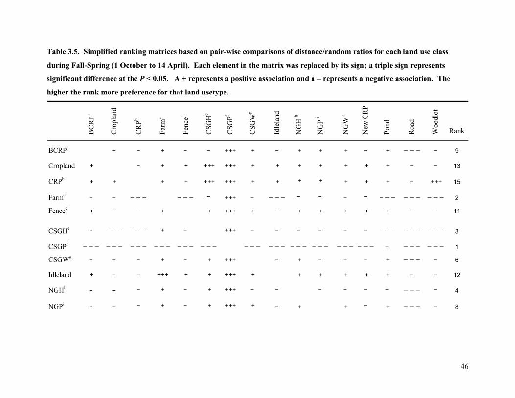
Table 3.5. Simplified ranking matrices based on pair-wise comparisons of distance/random ratios for each land use class

during Fall-Spring (1 October to 14 April). Each element in the matrix was replaced by its sign; a triple sign represents

significant difference at the P < 0.05. A + represents a positive association and a – represents a negative association. The

higher the rank more preference for that land usetype. B

CR

Pa

Cro

plan

d

CR

Pb

Farm

c

Fenc

ed

CSG

He

CSG

Pf

CSG

Wg

Idle

land

NG

H h

NG

P i

NG

W j

New

CR

P

Pond

Roa

d

Woo

dlot

Rank

BCRPa − − + − − +++ + − + + + − + − − − − 9

Cropland + − + + +++ +++ + + + + + + + − − 13

CRPb + + + + +++ +++ + + + + + + + − +++ 15

Farmc − − − − − − − − − +++ − − − − − − − − − − − − − − − − − 2

Fenced + − − + + +++ + − + + + + + − − 11

CSGHe − − − − − − − + − +++ − − − − − − − − − − − − − − − 3

CSGPf − − − − − − − − − − − − − − − − − − − − − − − − − − − − − − − − − − − − − − − − − − − 1

CSGWg − − − + − + +++ − + − − − + − − − − 6

Idleland + − − +++ + + +++ + + + + + + − − 12

NGHh − − − + − + +++ − − − − − − − − − − 4

NGPi − − − + − + +++ + − + + − + − − − − 8

46


BC

RPa

Cro

plan

d

CR

Pb

Farm

c

Fenc

ed

CSG

He

CSG

Pf

CSG

Wg

Idle

land

NG

H h

NG

P i

NG

W j

New

CR

P

Pond

Roa

d

Woo

dlot

Rank

NGWj − − − + − + +++ + − + − − + − − − − 7

New CRP + − − +++ − +++ + + − + + + + − − − − 10

Pond − − − + − + + − − + − − − − − − − 5

Road +++ + + +++ + +++ +++ +++ + +++ +++ +++ +++ − + 16

Woodlot − − − +++ + +++ +++ + + + + + + + − 14

a. Burned Conservation Reserve Program land. b. Conservation Reserve Program land. c. Farmstead. d. Woody Fencerow. e. Cool Season Grass Hayland. f. Cool Season Grass Pasture. g. Cool Season Grass Waterway. h. Native Warm Season Grass Hayland. i. Native Warm Season Grass Pasture. j. Native Warm Season Grass Waterway.

47

CHAPTER 4 - A Technique for Modeling Usable Space Based on

Distance

Abstract In recent years improvements in Geographic Information Systems and availability of remotely

sensed data have made it possible for biologists to use spatial modeling to predict and compare

landscape features with species abundance data as well as species specific presence/absence data.

Most current spatial models use coarse data such as Landsat satellite imagery to develop

statistical models. These types of modeling efforts provide biologists with a broad-scale

perspective of the landscape. Modeling at coarse spatial scales, does not however allow

biologists to examine fine-scale processes that may be affecting Northern Bobwhite (Colinus

virginianus) use of the landscape. I used a digitized land cover database of my study area in

southeastern Kansas to develop a space-use model based on distance to 5 habitat types. These

habitats included Conservation Reserve Program (CRP), Cropland, Idleland, Road, and Woody

Cover. I buffered each habitat at 30 m, 60 m, 90 m, 120 m, and 150 m, then used a weighted

overlay in ArcGIS to develop a predictive model of winter habitat that is compatible with the

biological adaptations of bobwhite (i.e. usable space) (Guthery 1997) within the study area.

When the model was compared with known covey locations, 84% of the locations were found in

the Medium and High space-use categories. This type of model can help biologists determine the

effects of management on movement of bobwhite as well as determining the usable space within

the management area. The technique can also be used at much finer scales such as within a patch

by mapping fine-scale patches within a particular field.

Introduction Remote sensing has been used by biologists to study the effects of landscape

configuration on a variety of wildlife. Roseberry and Sudkamp (1998) used Landsat TM satellite

imagery classified into 12 cover classes to examine the associations of habitat to population

levels in Illinois at the county and at the Breeding Bird Survey (BBS) route scales for northern

bobwhite (Colinus virginianus) . They found that 65% of Illinois’ landscape was unsuitable for

48

Northern Bobwhite (Roseberry and Sudkamp 1998). Schairer (1999) also used satellite imagery

to model areas of high and low bobwhite populations in Virginia and found it to be a good

predictor. Smith and Burger (2004) used Landsat TM to model abundance of bobwhite in

Mississippi. They found that the best predictive abundance model contained grass area and a

number of row crop patches.

Although these spatial models provide biologists with a broad view for comparing

whether an area may be suitable for bobwhite, they do not address issues of fine-scale such as

distance between habitats or the effects of small features such as fencerows on bobwhite usage.

Guthery (1997) and Williams et al. (2004) proposed that management for bobwhite should

emphasize the creation of usable space as opposed to creating edge as was proposed by Leopold

(1933) in his interspersion hypothesis. However Guthery (1997) also pointed out that the space-

use hypothesis is consistent with the interspersion hypothesis because bobwhites require at least

2 habitat types in close proximity in order to survive. Smith and Burger (2004) used IKONOS

satellite imagery with a spatial resolution of 4 m to model space-use of bobwhite by comparing

home ranges to random ranges. They found that their best model contained grass cohesion index,

row crop edge density, row crop and clumpiness index.

The problem with many of the current models for bobwhite is that they do not take into

account how far an animal will move. Schroeder (1985) proposed that optimum landscape for

bobwhite occurred where food, cover, and nesting resources were < 80 m apart. Perez et al.

(2002) found that mean flight distance for wild bobwhite was 46.5 m. The proximity of different

habitat types to each other is an important landscape characteristic for determining how usable a

particular habitat is for bobwhite. During the summer, vegetation growth patterns make the

landscape more usable, however during the winter, dormancy and agricultural activities can

severely limit the usability of the landscape and reduce movement of bobwhite.

In order to better manage the landscape, biologists need to be able to determine the

connectivity of the landscape for bobwhites as well as what areas will be preferred. Past

methods of modeling have only looked at indices of interspersion, habitat types, and landscape

metrics such as number of patches at broad spatial scales. These methods are a valuable tool

when planning and identifying general areas for management. However, when trying to

determine how a bobwhite may move or view the landscape these models are inadequate.

Bobwhites tend to prefer to walk from habitat to habitat but will use flight in order to transverse

49

larger areas or to escape predators. My objective was to develop a spatial modeling method that

took into account the movements of bobwhite within the landscape at finer scale than has been

previously presented.

Study Area The study area is a 64.75 km2 area located in the southwestern corner of Bourbon County,

Kansas, 3.2 km south of Uniontown. The area is also a demonstration area for the Southeastern

Kansas Quail Initiative sponsored by Kansas Department of Wildlife and Parks and other

cooperators. The landscape of the study area is one dominated by fescue in the east and cropland

in the west (Figure 4.1). Large tracts of cropland are located within the floodplains of streams.

Smaller tracts of cropland are scattered throughout the upland. There are narrow riparian forests

interconnected with small woodlots and linear wooded fencerows throughout the area. Many of

the fencerows consisted of Osage Orange (Maclura pomifera) > 50 years of age. Conservation

Reserve Program (CRP) lands are scattered throughout the uplands and in small patches in the

floodplains of streams and creeks. CRP consisted of native warm season grasses such as Big

Bluestem (Andropogon gerardii), Yellow Indiangrass (Sorghastrum nutans), and Switchgrass

(Panicum virgatum).

Methods Bobwhite were trapped from January through March and October through December in

2003 and 2004 using baited funnel traps on eight 0.64 km2 areas. All captured birds were sexed,

aged, weighed, and banded. Three to 6 random individuals within each covey weighing >150 g

were fitted within a necklace transmitter weighing <5 g. In late March all individuals caught

were equipped with radio transmitters to examine dispersal patterns.

Bobwhite with radio transmitters were located using a combination of 3 element yagi

antennas and 4 element null peak vehicle mounted antennas. Homing and short distance

triangulation (< 200 m) were conducted with hand-held antennas. UTM gridded aerial photos

were used to record location of bobwhite when homing and with short distance triangulation.

When bobwhite were flushed a Garmin Legend Global Positioning System (GPS) was used to

record the location within 5 m.

50

I on-screen digitized land cover in ArcView 3.3 (Environmental Systems Research

Institute, Inc. Redlands, CA) for the study area. I used 2002 Digital Orthophotos Quarter Quads

(DOQQ) as well as 2003 and 2004 National Agricultural Inventory Program (NAIP) digital color

aerial photos, from Kansas Data Access and Support Center (DASC), as base maps for land

cover analysis. Land cover was classified for 2003. Habitat was classified as developed

(farmstead, urban, rock quarry), roads, water, grassland (fescue hayfield, fescue pasture, and

fescue waterway), idleland, native grassland (native hayfield and native rangeland), woodland

(fencerows, grazed woodlot, and ungrazed woodlot), and CRP (new CRP, native waterway, and

established CRP). All areas were ground truthed in order to confirm habitat classifications.

I used ArcGIS 9.1 (Environmental Systems Research Institute, Redlands, California) to

separate the land cover layer into individual cover classes. I then buffered each land cover class

layer with 5 buffers at 30 m, 60 m, 90 m, 120 m, and 150 m. I reclassified land cover class and

buffers into 0-30 m, 31-90 m, and 91-150 m. I developed a usable space model in ArcGIS using

the weighted overlay function based on chapters 2 and 3. I used the percentage of radio locations

for the top 5 habitats for each weight and then ranked distance categories (Table 4.1). The model

produced a scale of 0 to 9; so I grouped these categories into 3 levels of usable space. I also

simulated hypothetical management on 3 sections within the study area to illustrate the effects on

usable space of adding fencerows 5-20 m wide and 60 m wide CRP buffers.

Results Usable space within the study area landscape was limited to areas containing woody

cover (Figure 4.2). When comparing covey locations with the usable space model, 82% of

locations occurred within the medium and high space areas (Figure 4.3). The usable space

model I developed will also allow biologists to examine the effects of creating more usable space

through adding woody cover and native grassland (Figures 4.4, 4.5, 4.6, and 4.7).

Discussion The usable space model I developed provides a way to examine the effects of habitat

configuration on movements of northern bobwhite. It allows managers and researchers to

examine how usable space is distributed within a landscape. Unlike other spatial models, the

model I developed, does not rely on percent composition of the landscape, instead it relies on

51

distance between each type of habitat. For instance, using Pattern Recognition (PATREC)

models in Illinois, Roseberry and Sudkamp (1998) found that bobwhite were associated with

landscapes that contained 30-65% row crops, 20-30% grassland at the county scale, and 40-70%

row crop and 12-25% grassland at the BBS route scale. Schairer (1999) found the optimum

landscape for bobwhite contained >20% row crop, > 20% early-successional habitat, and >12%

pasture/grass/hay.

My usable space model takes into account bobwhite preferences for particular habitat

juxtaposition. It does not treat all portions of the habitat equally. Woody cover is often used as

escape cover because it provides horizontal as well as vertical cover. On my study area, mean

distance to woody cover was 27.6 m (range 0 to 99 m). Kassinis and Guthery (1996) felt that

escape cover should be < 100 m from any point. My usable space model is more objective than

other models, because it provides biologists with the chance to identify areas that are highly

fragmented and test potential habitat management techniques to increase connectivity.

I did not use my spatial model to measure within patch use dynamics, but it would be

very easy to do this. For instance a patch containing scattered shrubs and trees could be modeled

to determine how the placement of fine-scale features could influence movement. This technique

could also be used to examine how placement of artificial structures such as brush piles or

creation of “covey headquarters” by planting shrubs might affect the usable space within the

patch. The model should be tested in a variety of different landscapes within the bobwhite range.

Spatial modeling can be an important tool in the management of habitat for bobwhite. It can also

provide information on behavior and how it might affect usable space.

Management Implications Being able to visualize the movement and space-use by bobwhite within a landscape or

within a patch can improve the ability of biologists to better manage the landscape. Williams et

al. (2004) recommend that biologists should promote creation of permanent cover for bobwhite

within the landscape. This has typically been done through CRP. However, CRP may not be

adequate for providing cover for bobwhite during the winter. The limited woody cover found in

most CRP often reduces the value of the field to the edges where woody cover is found. In many

agricultural landscapes, the edges of a field are hard edges rather the irregular “feathered” edges

52

that promote shrubby cover needed by bobwhites. Planting shrubs in groups or stripes through

out the CRP would most likely increase usable space within the field.

Clean farming practices removed many woody fencerows within the landscape. By

recreating these fencerows appropriate woody planting, edge feathering, or similar practices, and

tying them to programs such as the Habitat Buffers for Upland Birds (CP-33) could greatly

improve the usable space of the landscape for bobwhite as well as providing more connectivity.

53

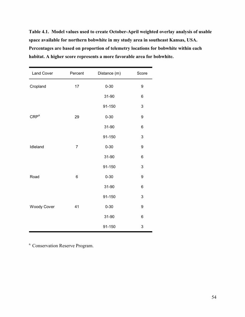
Table 4.1. Model values used to create October-April weighted overlay analysis of usable

space available for northern bobwhite in my study area in southeast Kansas, USA.

Percentages are based on proportion of telemetry locations for bobwhite within each

habitat. A higher score represents a more favorable area for bobwhite.

Land Cover Percent Distance (m) Score

Cropland 17 0-30 9

31-90 6

91-150 3

CRPa 29 0-30 9

31-90 6

91-150 3

Idleland 7 0-30 9

31-90 6

91-150 3

Road 6 0-30 9

31-90 6

91-150 3

Woody Cover 41 0-30 9

31-90 6

91-150 3

a. Conservation Reserve Program.

54

Figure 4.1. 2003 land cover of study area in southeastern Kansas, USA.

55

56

Figure 4.2. Winter weighted overlay model based on 5 habitat categories and 30-150m

buffers around each habitat to depict October to April usable space in southeastern,

Kansas, USA.

57

58

Figure 4.3. October to April usable space model with known covey locations in a portion of

southeastern Kansas, USA.

59

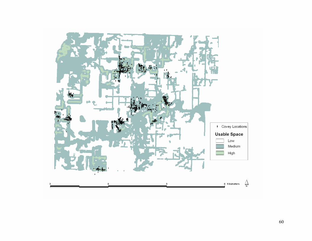
60

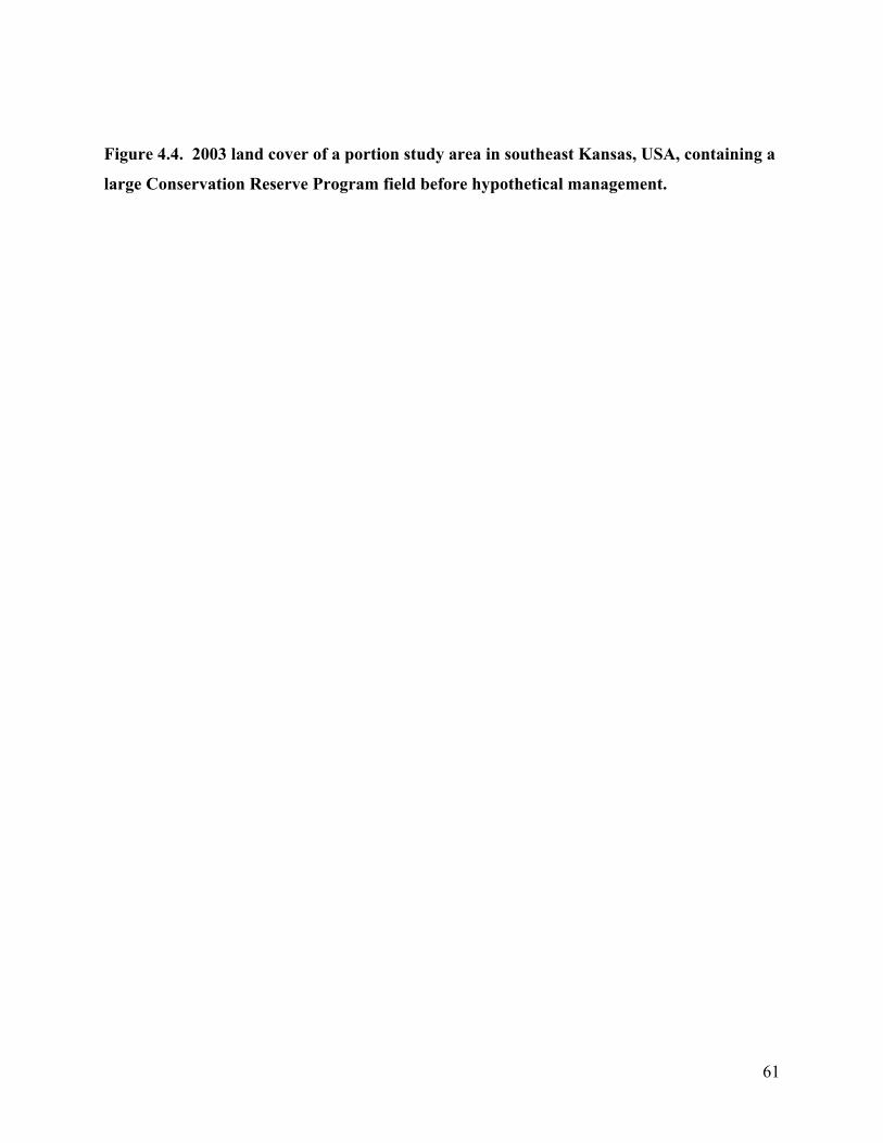
Figure 4.4. 2003 land cover of a portion study area in southeast Kansas, USA, containing a

large Conservation Reserve Program field before hypothetical management.

61

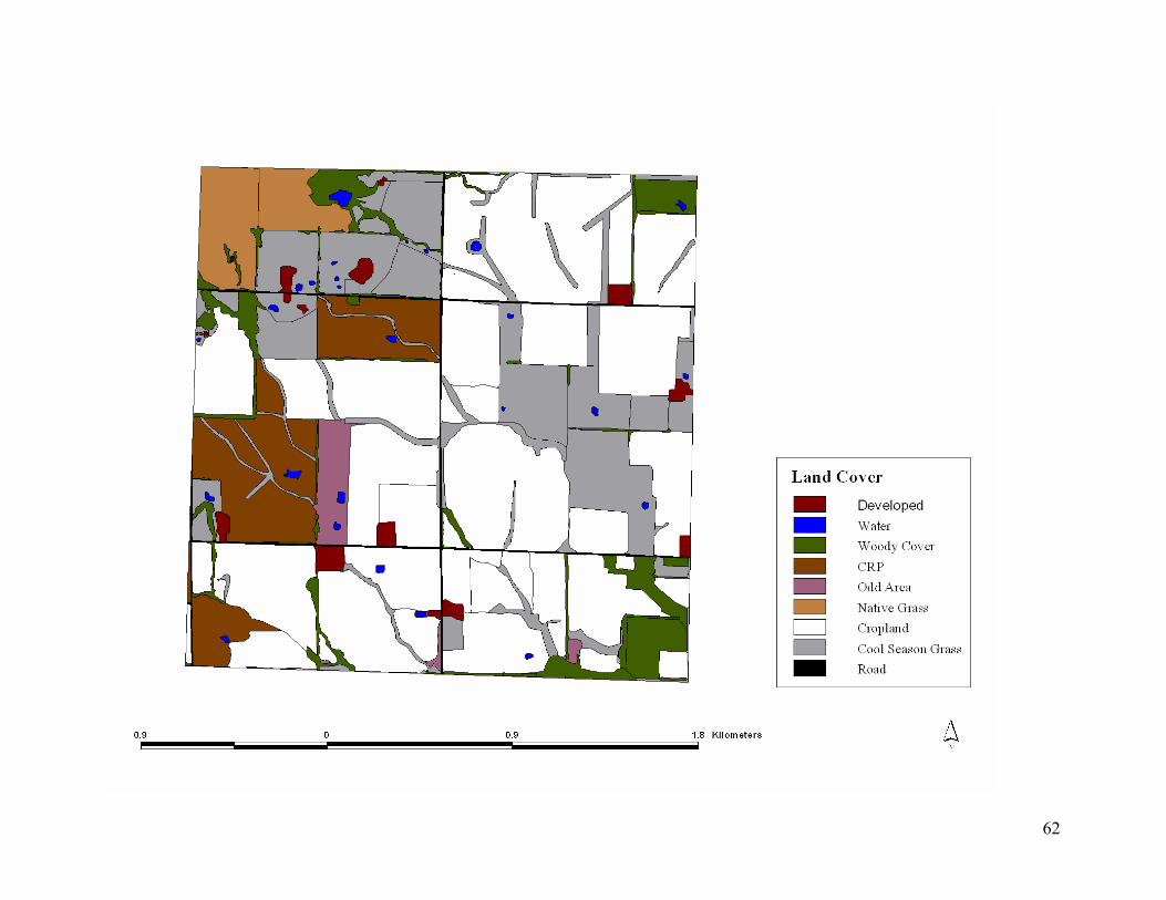
62

Figure 4.5. October-April usable space model based on 5 habitat categories and distance

from each habitat before hypothetical management on study area in southeastern, Kansas,

USA.

63

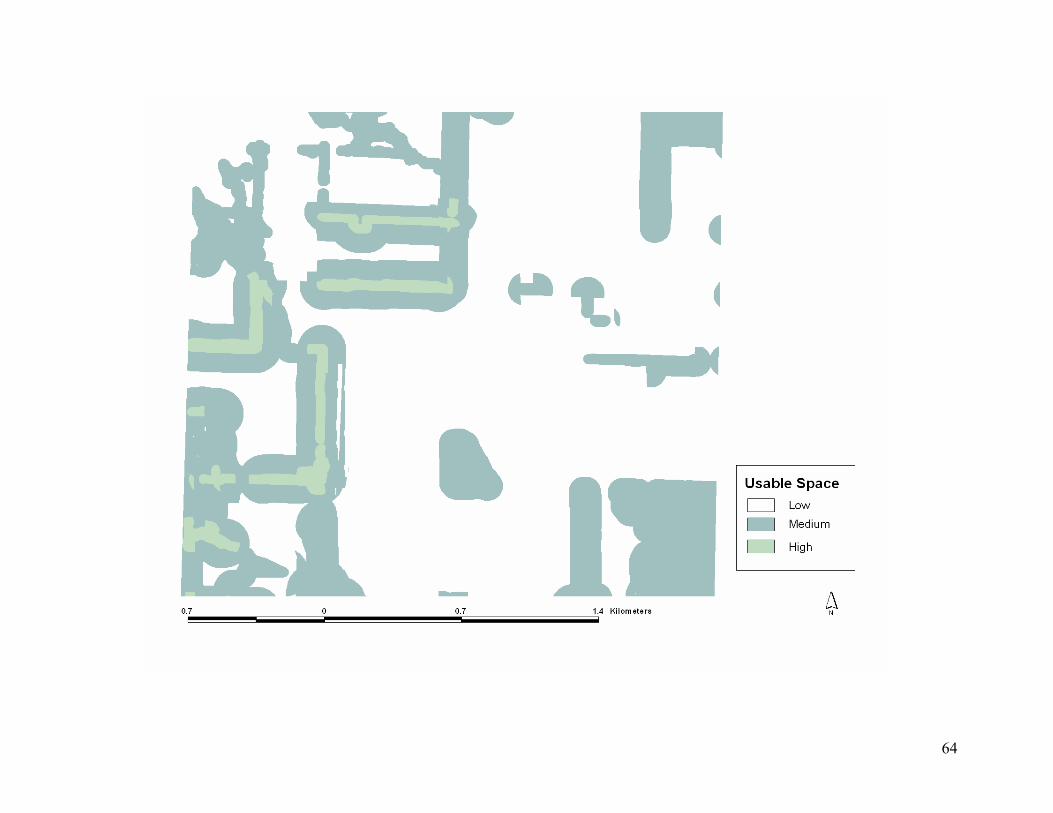
64

Figure 4.6. Portion of study area in southeastern Kansas, USA, with hypothetical

management in place which include fencerows and native warm season grass buffers.

65

66

Figure 4.7. October to April usable space model based on hypothetically managed portion

of study area in southeastern, Kansas, USA, based on 5 habitat categories and distance to

each habitat.

67

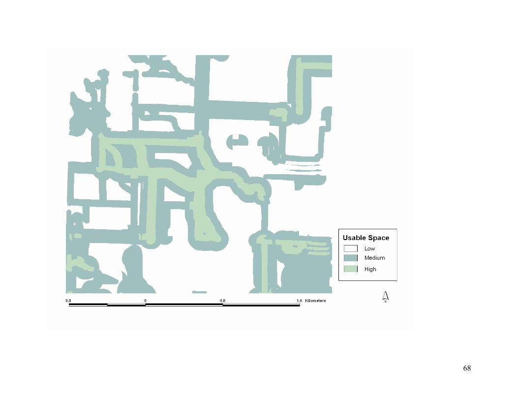
68

CHAPTER 5 - A Blueprint for Northern Bobwhite Habitat

Management in the Modern Agricultural Landscape

Abstract With the continued decline of northern bobwhite (Colinus virginianus) throughout much of its

range, biologists have struggled to find ways to reverse the decline. However management for

bobwhite has been focused on randomly created habitat at the individual patch scale. In today’s

modern agricultural landscape this type of management is not working. Management of habitat

for northern bobwhite needs to be conducted at multiple spatial scales. The first step in the

multi-scale management approach is to plan at the broad-scale using satellite imagery to

prioritize general areas and to select focus areas. Next, planning and management should move

to the focus area in order to increase usable space and connectivity within these areas. With the

multi-scale approach managers can continue managing patches at the fine-scale by use of the

many practices that create and maintain appropriate early-successional habitats. There is also a

need to take into account potential benefits that can be derived from cellulose feedstock

production for biofuels.

Introduction The widespread decline of northern bobwhite (Colinus virginianus) throughout much of

its range has often been attributed to changes in land cover and land use. These changes have

been on-going since the early 20th Century and has accelerated since WWII as agriculture has

become more modernized. Improvements in modern agriculture resulted in the practice of

“clean farming” which has drastically altered the landscape beyond that of times when bobwhite

were considered abundant.

With clean farming, fencerows and weedy areas are removed to create larger fields, and

odd areas are often mowed or eliminated to provide a “clean look”. With the modernization of

agricultural practices remaining hedgerows and fencerows are no longer disturbed for firewood

or fence post. Instead these areas have been removed or allowed to mature reducing their value

to bobwhite. Modern farming practices have also resulted in less productive areas being

69

abandoned and allowed to revert to their natural state. This resulted in good bobwhite habitat for

5 to 10 years until natural regeneration of trees reduced its value.

The destruction of bobwhite habitat by clean farming was recognized in the early 1930s

by Errington and Hamerstrom (1936). Other researchers have also recognized the effects of

“clean farming” on habitat (Goodrum 1949, Klimstra 1982, Brennan 1991). Unfortunately, as

the landscape has changed due to modern agricultural practices, the implementation of habitat

management for bobwhite has changed very little. There have been improvements on various

practices but the delivery of management is carried out without regard to landscape context of

bobwhite habitat use and bobwhite behavior and genetics.

Habitat management for bobwhite and many small game species has typically been

carried out at the field scale. At this scale management is based on improving habitat quality

rather than habitat quantity. At the field scale a biologist might recommend burning native warm

season grasses every 3 to 4 years to increase plant diversity and reduce litter depth which would

theoretically improve value of the area for nesting and brood rearing bobwhite. Often this is

paired with the idea that randomly distributing habitat throughout the landscape will result in

increased reproduction and survival. This type of management is further fueled by research

which is focused at that same scale and randomly distributed habitat improvements. Overarching

all of this is a lack of empirical knowledge of how certain practices affect bobwhite populations.

In many areas October-April landscape is much more fragmented than the April-

October landscape. This is due to farming practices and natural changes in vegetation due to

dormancy. For instance, in areas dominated by cool-season grasses such as tall fescue

(Schedonorus phoenix) and brome (Bromus inermis), grazing, haying, and winter dormancy

often result in a short vegetation that creates a landscape similar to a golf course. Agricultural

fields are often large and devoid of residual vegetation due to modern harvest techniques and

removal of fencerows to allow for larger equipment.

Barren winter landscapes reduce the ability of bobwhite coveys to interact and exchange

individuals. Williams et al. (2003) found that the optimal covey size was from 10 to 12

individuals, fewer than 10 resulted in decreased group survival, increased movement, and

decreased feeding efficiency. Larger groups had lowered individual survival, reduced feeding

efficiency, and increased movement (Williams et al. 2003). Maintenance of group size is fostered

by habitat with high connectivity and useable space.

70

Fragmentation reduces the ability of small coveys to recruit additional members as

winter mortality or harvest reduce their numbers and render the covey unable to maintain an

optimum size. The barren landscape results in large numbers of bobwhite being forced into

small areas unable to separate into coveys of the optimum size and once winter mortality or

harvest reduce these numbers below optimum size it decreases the ability to return to the

optimum size and covey extinction ensues.

Over the last 40 + years these covey dynamics and changes in the landscape have resulted

in the random distribution of habitat improvement (eg. scatter pattern) as impractical. Instead the

numbers have continued to decline. Williams et al. (2004) recommended that habitat

management for bobwhite needs to be based on larger areas. In this approach Williams et al.

(2004) recommended a shift from fine-scale habitat management to broader-scale ecological

evaluation and promoting usable space. The northern bobwhite requires a mix of early

successional habitats and because of this management should be conducted at multiple spatial

scales in order to both create usable space and maintain it.

In this paper I present a basic blueprint for carrying out management for bobwhite at

multiple spatial scales and describe the use of Geographic Information Systems (GIS) and

remote sensing for aiding in planning and management. I discuss the current short falls of the

Conservation Reserve Program (CRP) for providing habitat for bobwhite. I also discuss

potential for production of biofuels to create and maintain bobwhite habitat.

Habitat Management: A Multiple Scale Approach

Broad-scale Planning

In a multiple scale approach to habitat management, the key is to begin planning at a

broad-scale and work gradually toward a finer scale. The broad-scale allows for assessing the

landscape by determining habitat availability, connectivity, and interspersion. Advances in

Geographic Information Systems (GIS) and spatial analysis allow large areas to be assessed

relatively easily. Researchers have used satellite imagery to assess landscape features that affect

populations for a variety of species. Landsat satellites have a pixel resolution of 30 m x 30 m,

and SPOT has a pixel resolution of 20 m x 20 m which can be used to create maps with a scale of

about 1:100,000 based on their spatial resolution. Spatial modeling and satellite imagery have

been used little to guide habitat management. Satellite imagery has been found to be effective in

71

modeling presence/absence and habitat suitability for bobwhites. Roseberry and Sudkamp

(1998) used Landsat TM satellite imagery classified into 12 cover classes to examine the

associations of habitat to population levels in Illinois at county and the Breeding Bird Survey

(BBS) route scale. Schairer (1999) used satellite imagery to model areas of high and low

bobwhite populations in Virginia.

At a broad scale the percentage of various habitats has been found to be tied to

occurrence of bobwhite. The amounts of each habitat have varied for different studies but are

often relatively close. Roseberry and Sudkamp (1998) found that bobwhite in Illinois were

associated with a landscape which contained 30-65% row crops, 20-30% grassland at the county

scale, and 40-70% row crop and 12-25% grassland at the BBS route scale. Michener et al.

(1998) found in Georgia that the ideal landscape contained 30-35% row crop. Schairer found the

optimum landscape for bobwhite in Virginia contained > 20% row crop, > 20% early

successional habitat, and >12% pasture/grass/hay. This information can be used to further guide

management within a state. For instance, using their model Roseberry and Sudkamp (1998) were

able to determine that 63% of Illinois was considered unsuitable, 12.5% marginal, and 24.2%

potentially suitable. With this information it would be much easier to determine where

management could be most effective. It would also be possible to better understand what may be

lacking within other areas.

Using satellite imagery to guide management has a number of advantages as well as

disadvantages. The advantages of using Landsat TM satellite images include: are readily

available, inexpensive compared to other data, and cover relatively large areas (170 x 183

kilometers). Landsat satellite imagery is also multi-spectral meaning that the satellite is able to

measure reflectance of various wavelengths of visible and infrared light. This information can be

used to distinguish more readily between different habitat types. Classification of satellite

imagery can be done using a number of computer algorithms which allow for large areas to be

classified more uniformly.

With the coarseness of the imagery there are also a number of disadvantages. Small

habitat features such as roads, waterways, fencerows, or farmsteads are often difficult to

distinguish from the surrounding landscape. Also multiple habitat types may have similar

reflectance and result in being classified incorrectly. Classifications of the same imagery by 2

different individuals can result in different land cover classification maps. Understanding the

72

advantages and disadvantages of satellite imagery will help evaluate their limitation in setting up

a broad-scale habitat management plan.

Once the portions of a state or region that contains suitable habitat for bobwhite are

identified the next tier of planning can be initiated. At this level the broad-scale models

depicting suitable areas are analyzed visually to determine areas that already contain bobwhite

populations as well as areas of known concentrations of wildlife-friendly landowners. Wildlife-

friendly landowners are those that are often interested in trying any new habitat programs or

management practices that may increase wildlife populations on their land. This type of

landowner is also more likely to already have patches of habitat available for bobwhite as well as

a small number of bobwhites.

The modern agricultural landscape is often barren and extensively fragmented in the

winter. This fragmentation has resulted in small isolated metapopulations of bobwhite. The key

to developing “focus areas” is to create one large enough to encompass several metapopulations.

By including enough already established metapopulations, management can work to create

connectivity through increased usable space. The focus area should be large enough to provide

enough individuals during the spring dispersal to emigrate into new areas or into areas that have

been extirpated due to poor winter survival. By creating connectivity within the landscape,

usable habitat patches will not stay empty very long and gene flow will continue through the

metapopulations.

Williams et al. (2004) recommended that the size of a “focus area” should be > 2000 ha

although it might need to be adjusted based on size of farms, percent urbanization, and landscape

characteristics. In much of the Midwest, a much larger focus area would be needed in order to

account for large field sizes and providing enough coveys to survive the harsh winters. The ideal

focus area in much of the Midwest would be 6500 ha. With larger areas, pockets of habitat,

although isolated and susceptible to catastrophic events, should allow individuals to disperse out

into the landscape during dispersal and reoccupy new areas.

Focus Area Planning and Management

Once the focus area has been selected, the amount of usable space within the landscape

needs to be assessed as well as the connectivity of the landscape. In the chapter 4, I describe a

technique for modeling usable space using a weighted overlay technique in ArcGIS

73

(Environmental Systems Research Institute, Inc., Redlands, CA) and distance to each habitat.

With the increased availability of remote sensed imagery such as Digital Orthophotos Quads

(DOQQ) and National Agricultural Inventory Program (NAIP) colored-Infrared digital images

from Kansas Data Access and Support Center (DASC), with pixel resolutions of 1 m to 2 m, it is

possible to model habitat use of bobwhite at a relatively fine scale. These images allow a

1:12000 land cover map to be generated and to be used in planning management. At the 1:12000

scale smaller habitats such as fencerows, clumps of trees, or grassland patches under different

management regimes can be identified and mapped. When combined with ground truthing and

Global Positioning Systems (GPS) an accurate map can be generated. Land cover categories

should be designed to include difference in plant growth and management. Examples of habitat

types would include cool-season pasture, warm-season grass pasture, or CRP. When planning

management, biologists should work to identify current metapopulations within the focus area

and work to create corridors between these areas particularly during the winter when habitats are

the most limiting and covey size can play an important role in overwinter survival.

Habitat management at the focus area scale should include increasing fencerows, creating

woody cover, maintaining idleland (eg. early-successional habitat), and converting cool-season

grasses to native warm-season grasses. These processes would increase usable space within the

landscape as well as connectivity. Johnson et al. (1999) provides more information creating

connectivity within the landscape by creating corridors. Ideal fencerow size should be between

5-20 m with a buffer of 10-30 m of native warm-season grasses on at least one side. This buffer

will provide nesting cover, blocking winter snows from filling in the woody cover, and increase

thermal protection.

Although Williams et al. (2004) felt that management should focus on creating usable

space, I recommend that fine-scale management (within-patch management) also needs to be

addressed when managing for bobwhite. For instance past management of native warm-season

grasses has focused on burning every 3 to 4 years during late winter to early spring. The problem

with this in the current landscape is that it often results in complete removal of vegetation that is

critical for winter survival. Without this cover coveys may be forced into low quality habitat and

be depredated or lost to a winter storm. A better management tool would be to burn only portions

of the field in order to create a mosaic of burned and unburned habitat. Also planning of burns

should take into account what other landowners in the area maybe doing. This is where having a

74

close working relationship with landowners can strengthen management by not having too many

areas burned in a given area and season.

Thinking Outside the Box: Biofuels and Wildlife Habitat In recent years the term “biofuels” and “green fuels” have become the new buzz words

for using biomass to create a renewable energy either in the form of ethanol or for use in power

plants. Very little information is available on the effects of biofuels on wildlife and therefore the

exact effects can be difficult to predict. Biofuel production from biomass does provide an

alternative to creating habitat in areas where agriculture is more dominant.

Ethanol currently is derived through the fermentation of sugars found in corn. This

process relies on replanting of corn and heavy use of fertilizer to increase yields and maintain

productivity. The increased need for corn to produce ethanol can result in an increase in the loss

of idleland and grasslands as well as removal of fencerows to increase production. Corn based

ethanol production could become a threat to bobwhite populations as well as other wildlife

species. However, with improvements in technology, cellulose based ethanol may become the

mainstay for production of ethanol.

Cellulose ethanol is derived from fermenting sugars contained in cellulose and

hemicellulose. Cellulose based ethanol can be derived from a variety of different sources which

include herbaceous vegetation and woody vegetation. Another use of biomass from herbaceous

and woody vegetation is co-firing in electric power generation. In co-firing plant material is

mixed with coal in order to reduce carbon dioxide and sulfur emissions of coal-burning power

plants. The use of biofuels does have its downsides for wildlife habitat particularly if biologists

take the wait-and-see approach. One downside to cellulose ethanol production is the use of crop

residual vegetation which could result in increased need for lime and fertilizers and little residual

cover and waste grain left in the field. Also, most research currently has focused on

monocultures of switchgrass (Panicum virgatum) or other high biomass yielding plants grown in

monoculture which limit wildlife cover and food.

However, cellulose production from woody and herbaceous vegetation could be valuable

in creating and maintaining habitat for bobwhite in areas where agricultural crops provide little

value and reduce connectivity of the landscape. For instance, harvest of switchgrass for ethanol

production is based on increasing biomass yields as opposed to haying for cattle which is based

75

providing protein and increased digestibility. Lee and Boe (2005) found that best yields for

switchgrass plantings in central South Dakota occurred with one cutting in early August or

September. This late harvest could mean a reduction in nest loss due to harvest. Also, Lee and

Boe (2005) found that growth after harvest did not have an affect on yields the following year

which meant that it could provide conservation benefits such as providing a snow fence and

winter wildlife habitat. Murray (2002) found that pheasants preferred undisturbed areas of

switchgrass during the winter in Iowa and therefore recommended that biomass removal should

contain alternating strips of cut and uncut switchgrass.

Biofuel production whether for cellulose ethanol or co-firing in power plants could help

to create and maintain bobwhite habitat in the modern agricultural landscape. The preferred

woody vegetation for creating biofuels are fast growing and are vigorous resprouters such as

hybrid poplar (Populus spp), willow (Salix spp), or black locust (Robinia pseudoacacia). A

variety of other woody plants could also be used for biofuel sources which would be more

beneficial to bobwhite. These include dogwoods (Cornus spp), plum (Prunus spp), raspberry

(Rubus spp), or Osage-orange (Maclura pomifera).

One problem with Osage-orange (Maclura pomifera) and other fencerows is that they

have become dominated by large trees reducing their value to bobwhite which need shrubby

cover. It is time consuming and expensive to maintain fencerows or woodland edges as early

successional habitat. Harvest of wood for biofuels typically occurs on a 3 to 10 year rotation

which would be ideal for maintaining woody cover for bobwhite. By harvesting woody

fencerows for biofuels there would be an economic incentive for landowners to create, maintain,

and protect these areas. Rows of woody vegetation could be alternated with 60-150 m strips of

native warm-season grasses and forbs. This combination would provide winter and nesting

cover in close proximity as long as the area harvested was rotated in such a way to leave some

woody cover and residual grasses available at all times.

Conclusions Northern bobwhite populations have undergone a severe decline over the last 35+ years.

Past management techniques have shown limited ability in reversing the trend. Biologists need to

manage bobwhite and other wildlife at multiple spatial scales. By using remote sensing to

determine suitable areas for management and for planning management, biologists will be able to

76

use limited resources better. Also by concentrating management on focus areas will encourage

better relationships with landowners. Creating usable space and connectivity within the

landscape is key to increasing bobwhite populations. Fine-scale management should not be

ignored, but used as a tool to maintain the value of usable space within the landscape.

Biologists need to become more proactive in the development of programs that could

potentially benefit bobwhite and other wildlife by “thinking outside the box”. Currently biofuel

development and harvest schedules are being left up to the processors of the product and little

thought is being put into how it can be made a “greener” process with wildlife values. At a

landscape scale it maybe possible to provide connectivity as well as nesting and wintering habitat

by altering the harvest and diversity of plants used for biofuels without greatly affecting

production.

77

CHAPTER 6 - Summary and Conclusions

The primary goal of my research was to determine the effects of landscape configuration

on survival and habitat preference of northern bobwhite (Colinus virginianus). My research

shows that land cover can affect survival of bobwhites particularly in the Fall-Spring when

habitat is limited. Understanding how survival is affected by landscape pattern is an important

step in learning how to better manage for bobwhite. Woody cover played a key role in survival

of bobwhite during the Fall-Spring. The amount of woodland habitat was positively associated

with survival. Using Euclidean distance I also found that bobwhite had a preference for

locations in close proximity to woody cover. During the Fall-Spring covey locations were in

close proximity to larger patches of woody cover.

Williams et al. (2000) felt that low survival, reduced movement, and woody cover were

linked on their rangeland study area. Although woody cover in Williams et al. (2000) study

consisted of patches of shrubs distributed within the landscape. The importance of woody cover

with in my study area was strengthened by the negative association of Conservation Reserve

Program (CRP) land which often lacked woody cover with in the large patches of CRP. Woody

cover provides primary escape cover for bobwhite (Wiseman and Lewis 1981, Exum et al. 1982,

Roseberry and Klimstra 1984). Although woody cover structure often varies between studies the

importance of this habitat type in many studies shows the need to protect and create more

patches of woody cover particularly shrubby cover with in the landscape.

Cropland was also found to be an important predictor of survival during the Fall-Spring.

In my study cropland was positively associated with survival. However, Williams et al. (2000)

found avoidance of cropland in both their cropland study area and rangeland study area. In my

study area the positive association to cropland was most likely due to its close proximity to

woody cover as well as other wintering cover. In cropland areas woody cover was often

protected from grazing by cattle thus increasing its value to wintering bobwhite.

The lack of a connection between survival and habitat configuration during the Spring-

Fall may be due to the fact that the landscape in a fescue system is not as limited as during the

Fall-Spring which allows bobwhite to move more freely within the landscape. This is also

supported by my findings using Euclidean distance which shows bobwhite locations were in

close proximity to cool season grasses. In Missouri Call (2002) found that during the Spring-Fall

78

period survival was explained more by the behavior (nesting or brooding) than by habitat

association. Cook (2004) found that Spring-Fall survival was negatively associated with

hardwood cover and positively associated with cropland and linear habitat patches.

Biologists need to manage bobwhite and other wildlife at multiple spatial scales. This

idea is supported by the findings of chapters 2 and 3. Remote sensing will play a key role in

managing bobwhite at multiple spatial scales. Spatial models such as the usable space model that

I described in chapter 4 will allow managers to better understand how changes in the landscape

can affect the usability of different habitat types. By creating usable space and connectivity

within the landscape bobwhite populations will better be able to disperse into areas.

Biologists need to become more proactive in the development of programs that could

potentially benefit bobwhite and other wildlife by “thinking outside the box”. Currently biofuel

development and harvest schedules are being left up to the processors of the product and little

thought is being put into how it can be made a “greener” process with wildlife values. At a

landscape scale it maybe possible to provide connectivity as well as nesting and wintering habitat

by altering the harvest and diversity of plants used for biofuels without greatly affecting

production.

79

CHAPTER 7 - References

Aebischer, N. J., P. A. Robertson, and R. E. Kenward. 1993. Compositional analysis of

habitat use from animal radio-tracking data. Ecology 74:1313-1325.

Barnes, T. G., L. A. Madison, J. D. Sole, and M. J. Lacki. 1995. An assessment of

habitat quality for northern bobwhite in tall fescue-dominated fields. Wildlife Society

Bulletin 23:231-237.

Bingham, R. L. and L. A. Brennan. 2004. Comparison of type I error rates for statistical

analyses of resource selection. Journal of Wildlife Management. 68:206-212.

Brady, S. J., C. H. Flather, K. E. Church, and E. W. Schenck. 1993. Correlates of

northern bobwhite distribution and abundance with land-use characteristics in Kansas.

Proceedings of the National Quail Symposium 3:115-125.

Brennan, L. A. 1991. How can we reverse the northern bobwhite population decline?

Wildlife Society Bulletin. 19:544-555.

Burger, L. W., E. W. Kurzejeski, T. V. Dailey, and M. R. Ryan. 1990. Structural

characteristics of vegetation in CRP fields in northern Missouri and their suitability as

bobwhite habitat. Transactions of North American Wildlife and Natural Resource

Conference 55:74-83.

Burger, L. W., Jr., T. B. Dailey, E. W. Kurzejeski, and M. R. Ryan. 1995. Survival and

cause-specific mortality of northern bobwhite in Missouri. Journal of Wildlife

Management 59:401-410.

Burnham, K. P. and D. R. Anderson. 1998. Model selection and inference: a practical

information-theoretic approach. Springer-Verlag, New York, New York, USA.

Call, E. M. 2002. Application of logistic regression analysis of proportional hazard

modeling for investigating relationships between habitat and population

dynamics of bobwhite quail. Thesis, University of Missouri, Columbia, Missouri,

USA.

Church, K. E. and J. S. Taylor. 1992. Management and research of northern bobwhite

(Colinius virginianus) in North America: an overview. Gibier Faune Sauvage

9:787-796.

80

Cook, M. P. 2004. Northern bobwhite breeding season, dispersal, habitat use, survival in a

southeastern agricultural system. Thesis, University of Georgia, Athens, Georgia, USA.

Conner, J. W. and B. W. Plowman. 2001. Using Euclidean distances to assess

nonrandom habitat use. In: Radio tracking and animal populations. Eds J. J.

Millspaugh, and J. M. Marzluff.Academic Press, San Diego, CA, USA.

Conner, J. W., M. D. Smith, and L. W. Burger. 2003. A comparison of distance-based

and classification-based analysis of habitat use. Ecology 84:526-531.

Dinsmore, S. J., G. C. White, and F. L. Knopf. 2002. Advanced techniques for modeling

avian nest survival. Ecology 83:3476-3488.

Dixon, K. R. M. A. Horner, S. R. Anderson, W. D. Henriques, D. Durham, and R. J.

Kendall. 1996. Northern bobwhite habitat use and survival on a South Carolina

plantation during winter. Wildlife Society Bulletin 24:627-635.

Errington, P. L. and F. N. Hamerstrom. 1936. The northern bobwhite’s winter territory.

Iowa State College of Agriculture and Mechanical Arts Research Bulletin

2001:305-443.

Exum, J. H. R. W. Dimmick, and B. L. Dearden. 1982. Land use and bobwhite

populations in an agricultural system in west Tennessee. Proceedings National

Quail Symposium 2:6-12.

Garshelis, D. L. 2000. Delusions in habitat evaluations: measuring use, selection, and

importance. In research techniques in animal ecology: controversies and

consequences. Eds. Boitani, L. and T. K. Fuller. Columbia University Press, New

York, New York, USA. pp111-164.

Goodrum, P. 1949. Status of bobwhite in the United States. Transactions North American

Wildlife Conference 14:359-367.

Guthery, F. S. 1997. A philosophy of habitat management for northern bobwhites. Journal of

Wildlife Management 61:291-301.

Hobbs, N. T. and T. A. Hanley. 1990. Habitat evaluation: do use/availability data reflect

carrying capacity? Journal of Wildlife Management 54:515-522.

Hooge, P. N. and B. Eichenlaub. 2000. Animal movement extension to Arcview version

2.0. Alaska Science Center - Biological Science Office, U.S. Geological Survey,

Anchorage, AK, USA.

81

Johnson, C. W.; G. Bentrup, D. Rol, and T. C. Edwards. 1999. Conservation corridor planning

at the landscape level- managing for wildlife habitat. Washington, DC: USDA Natural

Resources Conservation Service.

Kassinis, N. I. and F. S. Guthery. 1996. Flight behavior of northern bobwhites. Journal

of Wildlife Management 60:581-585.

Klimstra, W. D. 1982. Bobwhite and changing land use. Proceedings National

Quail Symposium 2:1-5.

Kuvlesky, W. P., Jr., T. E. Fulbright, and R. Engel-Wilson. 2002. The impact of

invasive species on quail in the southwestern United States. National Quail

Symposium 5:118-128.

Lee, D. K. and A. Boe. 2005. Biomass production of switchgrass in central South

Dakota. Crop Science 45:2583-2590.

Leopold, A. 1933. Game Management. Charles Scribner’s Sons. New York. New York, USA.

Michener, W. K., J. B. Atkinson, P. F. Houlhoulis, P. M. Johnson, R. N. Smith, J. W.

Jones. 1998. Northern bobwhite quail: responses to landscape configuration.

Technical Papers, 64th Annual Meeting of the American Society for Photogrammetry

and Remote Sensing. Tampa, Florida, USA. 10pp.

Murray, L. D. 2002. Avian Response to harvesting switchgrass for biomass in southern Iowa.

Thesis, Iowa State University, Ames, Iowa, USA. 94pp.

Parsons, D. S. 1994. Nesting, Brood habitat, and utilization of planted food plots by northern

bobwhite in east Texas. Thesis, Stephen F. Austin State University, Nacogdoches, Texas,

USA.

Perez, R. M., D. E. Wilson, and K. D. Gruen. 2002. Survival and flight characteristics of

captive-reared and wild northern bobwhite in southern Texas. National Quail

Symposium 5:81-86.

Peterson, M. J., X. B. Wu, and R. Rho. 2002. Rangewide trends in landuse and northern

bobwhite abundance: an exploratory analysis. Proceedings of the National Quail

Symposiums 5:33-44.

Pollock, K. H., S. R. Winterstein, C. M. Bunck, and P. D. Curtis. 1989. Survival analysis in

telemetry studies: the staggered entry approach. Journal of Wildlife Management 53:1-6.

Roseberry, J. L. and W. D. Klimistra. 1984. Populations ecology of bobwhite. Southern Illinois

82

University press, Carbondale, Illinois, USA.

Roseberry, J. L. and S. D. Sudkamp. 1998. Assessing the suitability of landscapes for northern

bobwhite. Journal of Wildlife Management 62:895-902.

Rosene, W. 1984. The bobwhite quail, its life and management. Morris Communications

Corporation, Augusta, Georgia, USA.

Rotella, J. J., S. J. Dinsmore, and T. L. Shaffer. 2004. Modeling nest-survival data: a

comparison of recently developed methods that can be implemented in MARK and

SAS. Animal Biodiversity and Conservation 27:187-205.

Rempel, R. S. 2003. Patch Analyst. http://flash.lakeheadu.ca/~rrempel/patch/index.html

Sauer, J. R., J. E. Hines, and J. Fallon. 2005. The North American Breeding Bird Survey, Results

and Analysis 1966 - 2004. Version 2005.2. USGS Patuxent Wildlife Research Center,

Laurel, Maryland, USA.

Schairer, G. L. 1999. Landscape level evaluation of northern bobwhite habitats in eastern

Virginia using Landsat TM imagery. Thesis, Virginia Polytechnic Institute and State

University, Blacksburg, Virginia, USA. 126 pp.

Schroeder, R. L. 1985. Habitat suitability models: northern bobwhite. Biological Report 82

(10.104). U.S. Fish and Wildlife Service, Washington D.C., USA. 32pp.

Smith, M. D. and L. W. Burger, Jr. 2004. Multi-resolution approach to wildlife habitat

modeling using remotely sensed imagery. Proceedings of SPIE 5143:34-43.

Sole, J. D. 1995. Changes in vegetation and bobwhite quail and eastern cottontail rabbit use in a

converted fescue field. Transactions of the Kentucky Academy of Science 56:1-8.

Stoddard, H. L. 1931. The bobwhite quail: its habits, preservation, and increase. Charles

Scribner, New York, New York, USA.

Taylor, J. D., II and L. W. Burger, Jr. 2000. Habitat use by breeding northern bobwhites

in managed old-field habitats in Mississippi. National Quail Symposium 4:7-15.

Taylor, J. S., K. E. Church, D. H. Rusch, J. R. Cary. 1999. Macrohabitat effects on summer

survival, movements, and clutch success of northern bobwhite in Kansas. Journal of

Wildlife Management 63:675-685.

Van Horne, B. 1983. Density as a misleading indicator of habitat quality. Journal of Wildlife

Management 47:893-901.

Weigel, J. 2004. Nearest Neighbor 3.6. http://arcscripts.esri.com/details.asp?dbid=11765.

83

http://www.pwrc.usgs.gov/

http://arcscripts.esri.com/details.asp?dbid=11765

(June12, 2006).

White, G. C., and K. P. Burnham. 1999. Program MARK: survival estimation from

populations of marked animals. Bird Study (Supplement) 46:S120-S139.

White, G. C. and R. A. Garrott. 1990. Analysis of wildlife radio-tracking data. Academic Press,

San Diego, California, USA.

Williams, C. K. 2001. The effect of covey size on northern bobwhite winter population

ecology. Dissertation, University of Wisconsin, Madison, Wisconsin, USA.

Williams, C. K., R. S. Lutz, and R. D. Applegate, and D. H. Rusch. 2000. Habitat use and

survival of northern bobwhite (Colinus virginianus) in cropland and rangeland

ecosystems during the hunting season. Canadian Journal of Zoology 78:1562-1566.

Williams, C. K. R. S. Lutz, and R. D. Applegate. 2003. Optimal group size and northern

bobwhite coveys. Animal Behaviour 66:377-387.

Williams, C. K., F. S. Guthery, R. D. Applegate, and M. J. Peterson. 2004. The northern

bobwhite decline: scaling our management for the twenty-first century. Wildlife

Society Bulletin 32:861-869.

Wiseman, D. S. and J. C. Lewis 1981. Bobwhite use of habitat in tallgrass rangeland. Wildlife

Society Bulletin 9:248-255.

84

Documents

EFFECTS OF LANDSCAPE CONFIGURATION ON NORTHERN …